theory of production and cost
TRANSCRIPT

BABARIA INSTITUTE OF TECHNOLOGYSHREE KRISHNA EDUCATIONAL CHARITABLE TRUSTApproved by AICTE, NEW DELHI, Affiliated to GTU
PREPARED BY:1.SAURABH DAYAL SINGH 2.KARNIKA 3.VAIBHAV 4.VISHAL5.ASTHA6.SWAPNIL
SUBJECT : ENGINEERING ECONOMICS AND MANAGEMENTSUB.CODE : 2130004BRANCH : ELECTRICALSEMESTER : 03

Theory of Production
Theory of Production
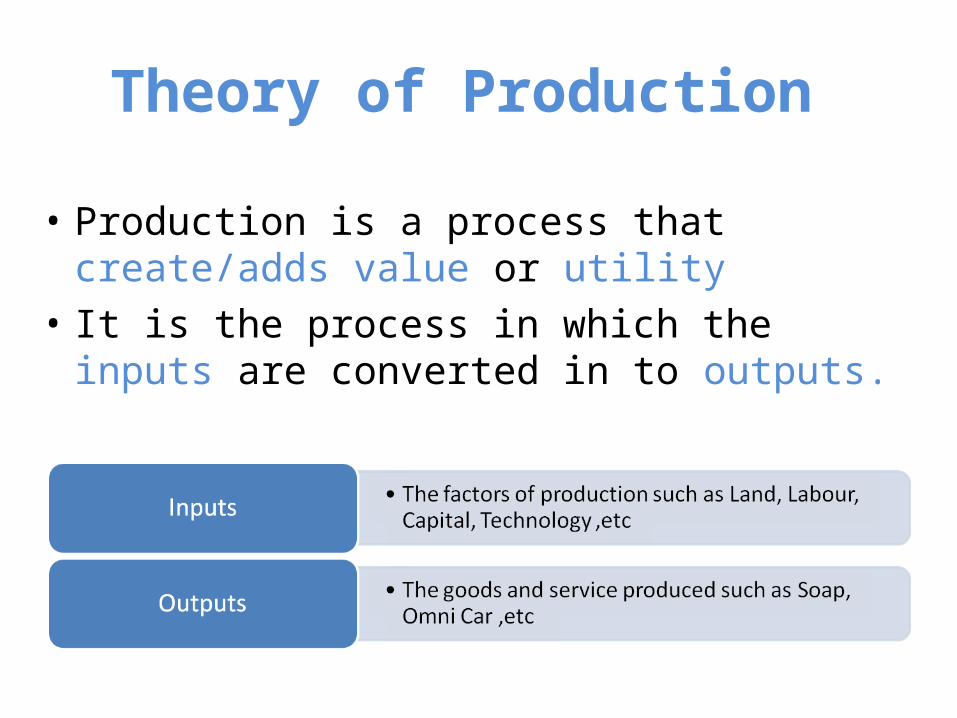
• Production is a process that create/adds value or utility
• It is the process in which the inputs are converted in to outputs.

Production Function
• Production function means the functional relationship between inputs and outputs in the process of production.
• It is a technical relation which connects factors inputs used
in the production function and the level of outputs
Q = f (Land, Labour, Capital, Organization, Technology, etc)

Production Function
• Production refers to the transformation of inputs or resources into outputs of goods and services. In other words, production refers to all of the activities involved in the production of goods and services, from borrowing to set up or expand production facilities, to hiring workers, purchasing row materials, running quality control, cost accounting, and so on, rather than referring merely to the physical transformation of inputs into outputs of goods and services.
• FOR EXAMPLE
1. A computer company hires workers to use machinery, parts, and raw materials in factories to produce personal computers.
2. The output of a firm can either be a final commodity or an intermediate product such as computer and semiconductor respectively.
3. The output can also be a service rather than a good such as education, medicine, banking etc.

Factors of Production

Inputs : Fixed inputs and Variable inputs
The factors of production that is carry out the production is called inputs.
Land, Labour, Capital, Organizer, Technology, are the example of inputs
Inputs Factors
Variable inputs Fixed Inputs

Inputs : Fixed inputs and Variable inputs
Fixed inputs
Remain the same in the short period .
At any level of out put, the amount is remain the same.
The cost of these inputs are called Fixed Cost
Examples:- Building, Land etc ( In the long run fixed inputs are
become varies)
Variable inputs
In the long run all factors of production are varies according to the volume of outputs.
The cost of variable inputs is called Variable Cost
Example:- Raw materials, labour, etc

Various concept of production
Total product (total physical product) = the total amount of output produced, in physical units .
Average product (AP) – total output divided by total units of input, means production per unit of input.
Marginal product – the extra product or output added by 1 extra unit of that input while other inputs are held constant.
L
TPAP
L
TPMP

Production with One Variable Input
Labour (L)
Capital (K)
Total Output (TP)
Average Product (AP)
0
1
2
3
4
5
6
7
8
9
10
10
10
10
10
10
10
10
10
10
10
10
Marginal Product
(MP)
0
10
30
60
80
95
108
112
112
108
100
Short run Production Function with Labour as Variable factor

Production with One Variable Input
Labour (L)
Capital (K)
Total Output (TP)
Average Product
(AP)
0
1
2
3
4
5
6
7
8
9
10
10
10
10
10
10
10
10
10
10
10
10
0
10
30
60
80
95
108
112
112
108
100
10
20
30
20
15
13
4
0
-4
-8
-
10
15
20
20
19
18
16
14
12
10
Marginal Product
(MP)
Short run Production Function with Labour as Variable factor

A
C
B
Total Product
Labor per month
3
4 8
84
3
E
Average product
Marginal product
Output per month
112
Labor per month
60
30
20
10
D

Law of Production Function
Laws of Variable proportion- Law of Diminishing Return ( Short run production function with at least one input is variable) .
Laws of Return scales – Long run production function with all inputs factors are variable.

Law of variable proportion:
Short run Production Function
• Production function with at least one variable factor keeping the quantities of others inputs as a Fixed.
• Show the input-out put relation when one inputs is variable .
“If one of the variable factor of production used more and more unit,keeping other inputs fixed, the total product(TP) will increase at an increase rate in the first stage, and in the
second stage TP continuously increase but at diminishing rate and eventually TP decrease.”

Production with One Variable Input
Labour (L)
Capital
(K)
Total Output (TP)
Average Product
(AP)
0
1
2
3
4
5
6
7
8
9
10
10
10
10
10
10
10
10
10
10
10
10
0
10
30
60
80
95
108
112
112
108
100
10
20
30
20
15
13
4
0
-4
-8
-
10
15
20
20
19
18
16
14
12
10
Marginal Product
(MP)
10
10
10
10
10
10
10
10
10
10
10
Land
First Stage
Second Stage
Third Stage
Short run Production Function with Labour as Variable factor

A
C
B
Total Product
Labor per month
3
4 8
84
3
E
Average product
Marginal product
Output per month
112
Labor per month
60
30
20
10
D
First Stage
Second Stage
Third Stage

Stages in Law of variable proportion
First Stage: Increasing return TP increase at increasing rate till the end of the stage. AP also increase and reaches at highest point at the end of the stage. MP also increase at it become equal to AP at the end of the stage. MP>AP
Second Stage: Diminishing return TP increase but at diminishing rate and it reach at highest at the end of the
stage. AP and MP are decreasing but both are positive. MP become zero when TP is at Maximum, at the end of the stage MP<AP.
Third Stage: Negative return TP decrease and TP Curve slopes downward As TP is decrease MP is negative. AP is decreasing but positive.

Law of return to scales
Long run Production Function • Long run production function when the inputs are changed in
the same proportion.
• Production function with all factors of productions are variable.
• Show the input-out put relation in the long run with all inputs are variable.
“Return to scale refers to the relationship between changes of outputs and proportionate changes in the in all factors of
production ”

Law of return to scales: Long run Production Function
Labour
Capital TP MP
2 1 8 8
4 2 18 10
6 3 30 12
8 4 40 10
10 5 50 10
12 6 60 10
14 7 68 8
16 8 74 6
18 9 78 4
Increasing returns to scale
Constant returns to scale
Decreasing returns to scale

1. Law of return to scales: Long run Production Function
Increasing returns to scale
Constant returns to scale
Decreasing returns to scale
Inputs 10% increase – Outputs 15% increase
Inputs 10% increase – Outputs 10% increase
Inputs 10% increase – Outputs 5% increase

Homogeneous production function
In the long run all inputs are variable. The production function is homogeneous if all inputs factors are increased in the same proportions in order to change the outputs.
A Production function Q = f (L, K )
An increase in Q> Q^ =f (L+L.10%, K+K.10% )- Inputs increased same proportion
Increasing returns to scale
Constant returns to scale
Decreasing returns to scale
Inputs increased 10% => output increased 15%
Inputs increased 10% => output increased 10%
Inputs increased 10% => output increased 8%
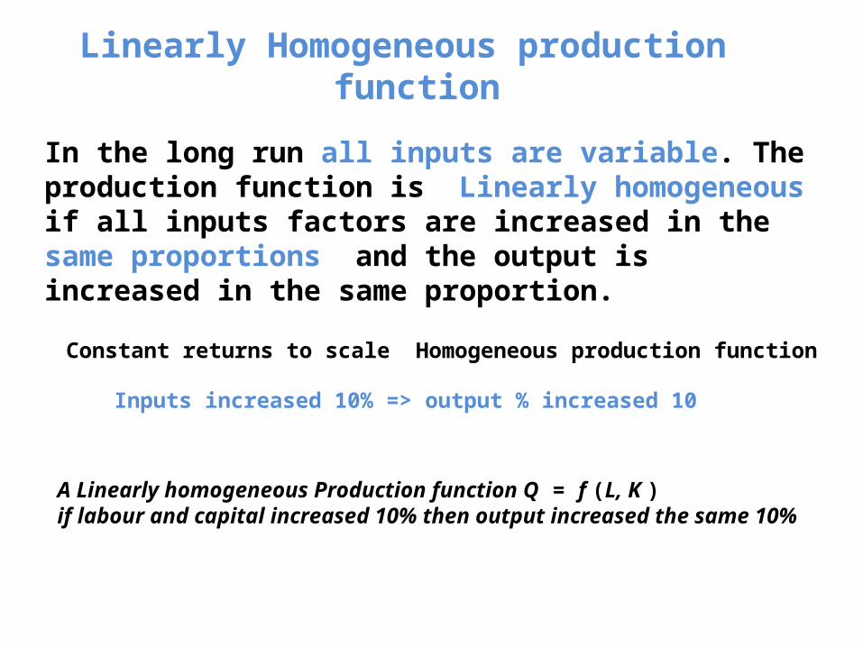
Linearly Homogeneous production function
In the long run all inputs are variable. The production function is Linearly homogeneous if all inputs factors are increased in the same proportions and the output is increased in the same proportion.
Constant returns to scale Homogeneous production function
Inputs increased 10% => output % increased 10
A Linearly homogeneous Production function Q = f (L, K ) if labour and capital increased 10% then output increased the same 10%

Linearly Homogeneous production function
A Linearly homogeneous Production function Q = f (L, K ) if labour and capital increased 10% then output increased the same 10%
100 unit output
200 unit output
300 unit output
400 unit output
%changes in factor Labour
%changes in factor Capital

Iosquants Combinatio
nLabour Capital Output level
A 20 1 100 unit
B 18 2 100 unit
C 12 3 100 unit
D 9 4 100 unit
E 6 5 100 unit
F 4 6 100 unit
An isoquants represent all those possible combination of two inputs (labour and capital), which is capable to produce an equal level of output .

100 unit output
Labour
Capital
Isoquants or equal product curve
Iosquants
An isoquants represent all those possible combination of two inputs ( Labour and Capital ), which is capable to produce an equal level of output.

100 unit output
Labour
Capital
Isoquants or equal product curve
Marginal Rate Technical Substitute(MRTS)
The slop of isoquant is known as Marginal Rate of Technical Substitution (MRTS). It is the rate at which one factors of production is substitute with other factor so that the level of the out put
remain the same.
MRTS = Changes in Labour / changes in capital

COST

Definitions of Costs
• It is the firm of the individual operating in a marketing has a influence on the market supply of the commodity.
• In order to make use of the various factor and non-factor inputs.
• In common, the amount spend on these inputs is called the cost of production.

Concept Of Cost
• MONEY COST : The amount spend in terms of money for the
production of the commodity is known as money cost .
• NOMINAL COST: It is the money cost of production.• REAL COST : It is the mental and physical and sacrifices
undergone with a view to producing a commodity.

•OPPORTUNITY COST :
The real concept of production of given commodity is the next best alternative sacrificed in order to obtain that commodity.
•SUNK COST :
•Firm buys a piece of equipment that cannot be converted to another use•Expenditure on the equipment is a sunk cost•Has no alternative use so cost cannot be recovered – opportunity cost is zero•Decision to buy the equipment might have been good or bad, but now does not matter

•IMPLICIT COST : It is the cost of self-owned resources such as salary of proprietor.
•EXPLICIT COST : * It is the paid-out cost. * It means payments made for the productive resources purchased.
• ACCOUNTING OR BUSINESS COST: Cash payments which firms make for factor and non-factor input depreciation other book keeping entries.
• SOCIAL COST: It is the amount of cost the society bears due to industrialization.
•ENTREPRENEUR’S COST: The cost of production in the sense of money cost or expenses of production.

•ACCOUNTING COSTS: These are the actual or outlay costs. These costs point out how much expenditure has already been incurred on a particular process or on production as such.
•ECONOMIC COSTS: These costs relate to future. They are in the nature of the incremental costs.
•DIRECT COSTS: Are the costs that have direct relationship with a unit of operation like a product, process or a department of the firm. Ex. Variable cost
•INDIRECT COSTS: Are those whose source cannot be easily and definitely traced to a plant, a product, a process or a department. Ex. Fixed cost
•CONTROLLABLE COSTS: Are those which are capable of being controlled or regulated by executive vigilance and therefore, can be used for assessing executive efficiency.
•NON-CONTROLLABLE COSTS: Are those which cannot be subjected to administrative control and supervision.

SHORT-RUN COSTS
In the short run at least one factor of production is fixed.Output can be varied only by adding more variable factors. FIXED COST:Remains constant.Also known as short-run cost.This cost includes: *Cost on managerial staff. *Expenditure on depreciation. *Maintenance cost of the factory.VARIABLE COST:Vary directly with the level of output Used in the actual production process.Functions of output changes.Eg: Cost of raw-materials. Cost in direct labour. TOTAL COST: Sum of total fixed cost and total variable cost. TC=TVC+TFC. TVC=0, when the output is zero and increases with increase in the output.

AVERAGE COST
They are of three types. AVERAGE FIXED COST: It is the per-unit cost of the fixed factors. AFC=TFC/Q.
AVERAGE VARIABLE COST: It is the per-unit cost of the variable factors. AVC=TVC/Q.
AVERAGE TOTAL COST: * It is the total cost divided by the number of units produced. * Sum of average fixed cost and average variable cost. ATC=TC/Q AC=AFC+AVC.

CHANGE IN VARIABLE COST

CHANGE IN FIXED COST-NO EFFECT
MARGINAL COST:
Change in the total cost resulting from the unit change in the quantity produced.
MC=Change in Q/Change in TC.

SHORT RUN COSTS OF PRODUCTION

It is a period of time during which the quantities of all factors, variable as well as fixed can be adjusted. LONG-RUN AVERAGE COST CURVE: Slopes downwards. Larger scope of specialization of labour. Increasing use of specialized machinery. Other technological management.
LONG-RUN MARGINAL COST CURVE: Cuts the LRAC at the lowest point. It is equal to the LRAC when LAC is neither rising nor falling.
LONG-RUN COST CURVES

LONG-RUN COST CURVES
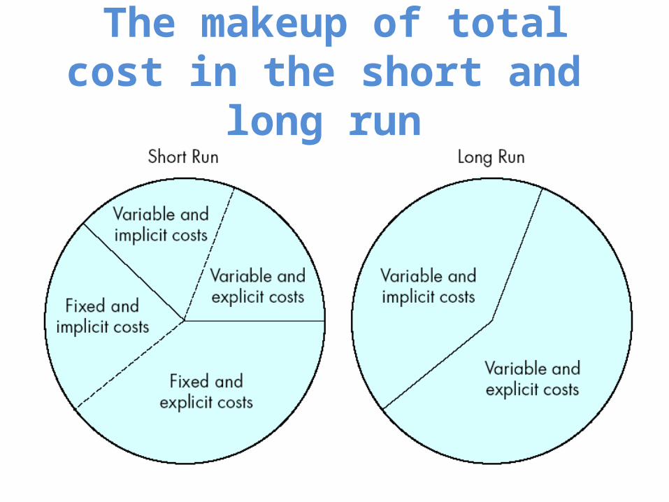
The makeup of total cost in the short and long run

From the law of variable proportions, theory of production and theory of cost it may not be understood that there is no hope for raising the standard of living of mankind.
The fact, however, is that we can suspend the operation of diminishing returns by continually improving the technique of production through the progress in science and technology.
CONCLUSION
REFRENCES• www.wikipedia.com• www.slideshares.com• www.microeconomics.com
• Adhikary, M (1987), Managerial Economics (Chapter V), Khosla, Publishing House, Delhi.
• T.S Grewal, Introductory Microeconomics• Introduction To Microeconomics, CBSE class XII

THE END