theory of nonstationary linear filtering in the …-1- march 28, 1997 theory of nonstationary linear...

-1- March 28, 1997

Theory of nonstationary linear filtering in the Fourier domain with application to time variant filtering

Gary F. Margrave, The CREWES Project, The University of Calgary

ABSTRACT A general linear theory is presented which describes the extension of the convolutional

method to nonstationary processes. This theory can apply any linear, nonstationary filter, with arbitrary time and frequency variation, in the time, Fourier, or mixed domains. The filter application equations and the expressions to move the filter between domains are all ordinary Fourier transforms or generalized convolutional integrals. Nonstationary transforms such as the wavelet transform are not required. There are many possible applications of this theory including: the one-way propagation of waves though complex media, time migration, normal moveout removal, time variant filtering, and forward and inverse Q filtering.

Two complementary nonstationary filters are developed by generalizing the stationary convolution integral. The first, called nonstationary convolution, corresponds to the linear superposition of scaled impulse responses of a nonstationary filter. The second, called nonstationary combination, does not correspond to such a superposition but is shown to be a linear process capable of achieving arbitrarily abrupt temporal variations in the output frequency spectrum. Both extensions have stationary convolution as a limiting form and, in the discrete case, can be formulated as matrix operations.

Fourier transformation shows that both filter types are nonstationary convolution integrals in the Fourier domain as well. This result is a generalization of the convolution theorem for stationary signals because, as the filter becomes stationary in one domain, the convolution integral in the other domain collapses to a scalar multiplication. For discrete signals, stationary filters are a matrix multiplication of the input signal spectrum by a diagonal spectral matrix while nonstationary filters require off-diagonal terms. For quasi-stationary filters, a computational advantage is obtained by computing only the significant terms near the diagonal.

Unlike stationary theory, a mixed domain of time and frequency is also possible. In this context, the nonstationary filter is applied simultaneously with the transform from time to frequency or the reverse. Nonstationary convolution becomes a generalized forward Fourier integral and nonstationary combination is a generalized inverse Fourier integral.

INTRODUCTION A common occurrence in geophysical research and data processing is the need to apply

convolutional operators which somehow depend on both variables of a Fourier transform pair. Time variant filtering is a typical example. Filters are convolutional operators which shape the spectrum1 of a time series therefore a time variant filter must both shape the spectrum and change with time. Another example is the vertical extrapolation of a wavefield through a laterally variable velocity structure. The kinematics of wavefield

1 In this paper, the word “spectrum”, without any qualifiers, is completely synonymous with “Fourier Transform”. Thus the spectrum of g(t) is equivalent to the Fourier transform of g(t) and is a complex valued function of frequency. “Amplitude spectrum” refers to the absolute value of the spectrum (often called the magnitude spectrum) while “phase spectrum” refers to the imaginary part of the complex logarithm of the spectrum. “Fourier spectrum” is identical to spectrum and is used occasionally for stylistic variation.

Margrave Nonstationary Filter theory

Manuscript # 96198 -2- March 28, 1997

extrapolation can be handled by a phase shift which depends on horizontal wavenumber and velocity; or equivalently, by a spatial convolution over the lateral coordinate. Thus, when velocity varies laterally, a convolution is desired which depends on both the lateral coordinate and the horizontal wavenumber.

Ordinary convolutional filters are incapable of directly handling these and other similar situations since they assume a "stationary" impulse response. By stationary it is meant that the filter's properties do not change with time or space. Since the convolution theorem (see any good text on signal processing, for example Karl, 1989, p 88, or Brigham ,1974, p 58) states that stationary convolution is a multiplication of Fourier spectra, it is commonly assumed that Fourier methods are also incapable of handling nonstationary filters. However, a more fundamental result is that a continuous function's Fourier transform is a complete description of the function. It follows that if nonstationary filtering can be done at all, it can be done in the Fourier domain.

Nonstationary filtering is done routinely in seismic data processing (and elsewhere). Wavefield extrapolation through laterally varying media (i.e. depth migration) is typically done with either spatially varying finite difference techniques (see Claerbout, 1985) or spatially variant convolutional operators (Berkhout 1985, section X, Holberg, 1988). Gazdag and Squazzero (1984) have accomplished wavefield extrapolation in this setting with the PSPI method which amounts to lateral interpolation between wavefields extrapolated with stationary Fourier phase shifts. Wapenaar (1992), Wapenaar and Dessing (1995), and Grimbergen et al. (1995) present a Fourier method of wavefield extrapolation through laterally variable media which is a nonstationary filter of precisely the type described here. Black et al. (1984) presented a Fourier domain expression for a similar wavefield extrapolation method. Many other seismic processing techniques, while not commonly formulated as nonstationary filters, can be recast in this way. For example, NMO (Normal Moveout) removal can be accomplished as a time variant time shift (i.e. a time variant static correction). Since a time shift can be done in the Fourier domain as a phase shift, NMO removal can be described as a phase shift filter whose phase is nonstationary. It then follows that Kirchhoff time migration is also a form of nonstationary filtering. Yet another related example is the frequency domain mapping from (ω,kx) space to (kz,kx) space, which is the key step in f-k migration (Stolt, 1978) and is mathematically analogous to NMO removal.

Time variant filtering has been implemented in various ways. The simplest method is to apply stationary filters to different overlapping trace segments and to interpolate them into a unified result (Yilmaz, 1986, p25-26). Pann and Shin (1976) show that the interpolation results in an embedded spectrum which is not the desired one in the overlap zones. Pann and Shin (1976) and later Scheuer and Oldenburg (1988) implemented time varying bandpass filters with an efficient algorithm which uses the theory of complex signals (Taner et al. 1979) as a basis. These methods achieve a filter with a continuously variable pass band and a possible nonstationary phase rotation. However, they are limited in the shape of the amplitude and phase spectra and the rate of time variation. Park and Black (1995) present an excellent summary of previous work as well as a new method based upon Fourier transform scaling laws. Their method is able to achieve a more rapid and flexible temporal variation of the bandpass characteristics. A third class of time variant filters are implemented as recursive algorithms (Stein and Bartley, 1983). These methods can be quite strongly nonstationary but have only very limited phase options and, for short recursions, may produce amplitude spectral responses far from the desired ones (see Park and Black, 1995, or Scheuer and Oldenburg, 1988 for summaries).

Also important in this context are nonstationary filters based on nonstationary transforms such as the wavelet transform (Chakraborty and Okaya, 1994, Kabir et al., 1995, Chakraborty and Okaya, 1995), the short time Fourier transform, or the Gabor transform (Gabor, 1946). (For a general discussion on nonstationary transforms see



Kaiser, 1994). These methods are capable of achieving quite general filtering effects and there will certainly be increased usage of nonstationary transforms in the next few years. Nonstationary transform techniques are perhaps most important when the nonstationary filter must be determined from a spectral analysis of the data. However, there are many situations when the filter parameters are either known apriori (as in depth migration) or they are easily estimated without a nonstationary transform (as is the often case with time variant filtering). Given such an apriori nonstationary filter specification, it is shown here that the filter can be efficiently applied in the time domain or the ordinary (stationary) Fourier domain by a generalization of convolutional concepts. It may be sensible to use nonstationary transforms to design filters which are then applied with the techniques presented here.

In the next section, a general mathematical theory for nonstationary filtering is presented. The key theoretical results are simply stated with derivations provided in the appendices. As the major points are detailed their meaning is discussed and illustrated with a running example of a forward constant Q filter. The mathematics is developed using continuous signal theory and integral calculus. The theory can be translated to the matrix notation appropriate for discrete signals in the same manner as is done for stationary theory (see Karl, 1989, for a tutorial). Generally, one dimensional functions become discrete vectors, two dimensional functions become discrete matrices, and integrals are computed through matrix multiplications. Though this transition is obviously necessary for practical applications (including the examples presented here), it is left implied for simplicity and clarity of exposition.

The basis for the theory is an extension of the stationary convolutional integral such that it contains stationary filtering as an obvious limit and that it forms the scaled superposition of nonstationary impulse responses. This process is termed nonstationary convolution. In addition, an alternate extension for the stationary convolution integral is developed which is called nonstationary combination and, though it does not correspond to the scaled superposition of impulse responses, it still has stationary convolution as a limiting form. Unlike nonstationary convolution, nonstationary combination is found to be capable of producing an output spectrum which varies in time with arbitrary abruptness.

Both processes are then reformulated in the Fourier domain. When represented as matrix operations appropriate for digital filters, stationary filters are shown to be achieved as the multiplication of the input signal spectrum by a diagonal matrix which has the filter spectrum on the diagonal. As the filter becomes nonstationary, the spectral filter matrix generates off diagonal terms to describe the filter variation.

In addition to these two traditional domains for filter application, two mixed domains of time and frequency are then explored. Nonstationary convolution is recast as a generalized forward Fourier integral of the product of the nonstationary filter and the time domain signal which yields the spectrum of the filtered trace. Alternatively, nonstationary combination may be expressed as a generalized inverse Fourier integral of the product of the nonstationary filter and the spectrum of the input trace. This results in a time domain output signal.

Following the theoretical development, an extensive exploration of the techniques is presented through the example of a time variant filter. A smoothly time variant bandpass specification is applied to a spike sequence using three different phase spectra: zero, minimum, and constant phase changing linearly with time. The nonstationary filter is shown in each domain and nonstationary convolution is compared with nonstationary combination. Then a second example, in which a bandpass specification changes abruptly, is given to better contrast convolution and combination.



PRINCIPLES OF NONSTATIONARY LINEAR FILTERING

Generalization of stationary convolution It is well understood that stationary convolutional filters are completely described by

their impulse response (Papoulis, 1984, p. 15-18). This means that if the response of a linear, stationary process to a unit impulse input at any particular time is known, then the response to an impulse at any other time is identical, except for a causal delay (principle of stationarity), and a scale factor. The response to more complicated inputs is the scaled superposition of many identical impulse responses. The process of forming the scaled superposition is called convolution. If h(τ) represents an input signal and a(u) is an arbitrary linear stationary filter, then g(t), the filtered output, is given by the convolutional integral

g(t) = a(t – τ)h(τ)dτ– ∞

∞

≡ a(t) • h(t) . (1)

This familiar expression is presented again here so that the nonstationary results can be seen as reasonable generalizations of the stationary case. The presence of a(t – τ) in equation (1) means that the actual response of the filter to an impulse at time τ0 is

a(t – τ0) which is a delayed version of the filter; the delay being a consequence of a causality constraint. Thus, though a(u) is called the filter impulse response, the actual response to a general impulse is a(t – τ0) . (It is a simple matter to prove that

h(t) • a(t) = a(t) • h(t) and thus h(t) could equally well be delayed; though, the form of equation (1) is better suited to generalization for nonstationary filters.)

The generalization of equation (1) to nonstationary systems can be done in a number of ways though some are more intuitively appealing than others. Pann and Shin (1976) and Scheuer and Oldenburg (1988) have chosen to replace a(t – τ) with a(t,τ) which refers to an arbitrary real function of t and τ . Though correct, this formalism is perhaps overly general and does not suggest a simple relation to the stationary form. Instead, consider replacing a(t – τ) with a(t – τ,τ) . This notation preserves the concept of delaying the filter response to account for causality and incorporates explicit τ dependence to describe the filter variation with time. Also the stationary limit is simply obtained by letting the τ dependence become constant. Alternatively, a(t – τ) could also be replaced with a(t – τ,t) with similar appeal. Intuitively, a(t – τ,τ) and a(t – τ,t) differ in that the former prescribes the temporal variation of the nonstationary filter as a function of input time, τ , while the latter uses output time, t , for the same purpose. The choice of which form to use and the comparison of results which follow from both is a central theme of this paper.

The meaning of these two alternate functional forms (a(t -τ, τ) and a(t -τ, t)) may be clarified by considering the matrix equivalent to discrete convolution. Given sampled versions of g(t), h(t), and a(t), then the convolutional process can be represented as

gk =∆t ak – jh jΣj

. (2)

Here ∆t is the temporal sample interval and the range of summation is left implied and is assumed to be over all appropriate values. This expression can be recast as a matrix operation by representing g and h as column vectors and building a special "convolutional matrix" with a(t) (see Strang, 1986, for an excellent discussion). The result is



g0

g1

g2

g3

=

a0 a–1 a– 2

a1 a0 a–1

a2 a1 a0

a3 a2 a1

h 0

h 1

h 2

h 3

. (3)

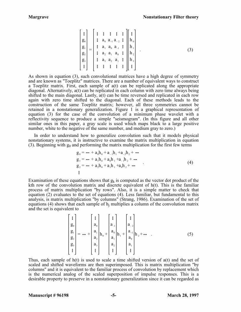
As shown in equation (3), such convolutional matrices have a high degree of symmetry and are known as "Toeplitz" matrices. There are a number of equivalent ways to construct a Toeplitz matrix. First, each sample of a(t) can be replicated along the appropriate diagonal. Alternatively, a(t) can be replicated in each column with zero time always being shifted to the main diagonal. Lastly, a(t) can be time reversed and replicated in each row again with zero time shifted to the diagonal. Each of these methods leads to the construction of the same Toeplitz matrix; however, all three symmetries cannot be retained in a nonstationary generalization. Figure 1 is a graphical representation of equation (3) for the case of the convolution of a minimum phase wavelet with a reflectivity sequence to produce a simple "seismogram". (In this figure and all other similar ones in this paper, a gray scale is used which maps black to a large positive number, white to the negative of the same number, and medium gray to zero.)

In order to understand how to generalize convolution such that it models physical nonstationary systems, it is instructive to examine the matrix multiplication in equation (3). Beginning with g0 and performing the matrix multiplication for the first few terms

g0 = + a0h0 + a– 1h1 +a– 2h2 +g1 = + a1h0 + a0h 1 +a– 1h 2 +g2 = + a2h0 + a1h 1 +a0h 2 + . (4)

Examination of these equations shows that gk is computed as the vector dot product of the kth row of the convolution matrix and discrete equivalent of h(t). This is the familiar process of matrix multiplication "by rows". Also, it is a simple matter to check that equation (2) evaluates to the set of equations (4). Less familiar, but fundamental to this analysis, is matrix multiplication "by columns" (Strang, 1986). Examination of the set of equations (4) shows that each sample of hj multiplies a column of the convolution matrix and the set is equivalent to

g0

g1

g2

g3

= +

a0

a1

a2

a3

h0 +

a–1

a0

a1

a2

h1 +

a– 2

a–1

a0

a1

h 2 + . (5)

Thus, each sample of h(t) is used to scale a time shifted version of a(t) and the set of scaled and shifted waveforms are then superimposed. This is matrix multiplication "by columns" and it is equivalent to the familiar process of convolution by replacement which is the numerical analog of the scaled superposition of impulse responses. This is a desirable property to preserve in a nonstationary generalization since it can be regarded as



a direct consequence of Green's function analysis for linear partial differential equations (Morse and Feshbach, 1953). The implication is that an exact solution of a constant coefficient, linear, partial differential equation, when expressed as the (stationary) convolution of a Green’s function with a distributed source or boundary value (such as the Kirchhoff integral from acoustics), may be approximately extended to variable coefficients as a nonstationary convolution. The meaning of “approximate” here will vary from case to case; in the case of acoustic wave propagation it usually means that reflections are neglected resulting in a one-way wave propagator (Wapenaar and Dessing, 1995).

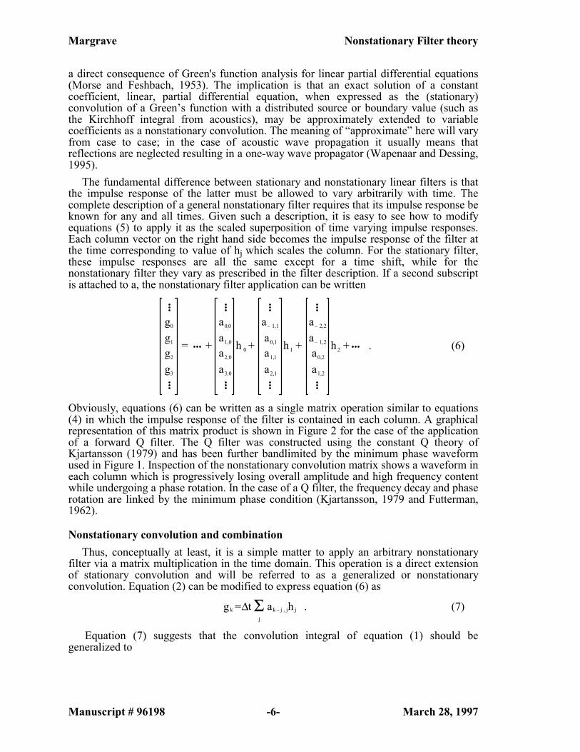
The fundamental difference between stationary and nonstationary linear filters is that the impulse response of the latter must be allowed to vary arbitrarily with time. The complete description of a general nonstationary filter requires that its impulse response be known for any and all times. Given such a description, it is easy to see how to modify equations (5) to apply it as the scaled superposition of time varying impulse responses. Each column vector on the right hand side becomes the impulse response of the filter at the time corresponding to value of hj which scales the column. For the stationary filter, these impulse responses are all the same except for a time shift, while for the nonstationary filter they vary as prescribed in the filter description. If a second subscript is attached to a, the nonstationary filter application can be written

g0

g1

g2

g3

= +

a0,0

a1,0

a2,0

a3.0

h 0 +

a– 1,1

a0,1

a1,1

a2,1

h1 +

a– 2,2

a– 1,2

a0,2

a1,2

h2 + . (6)

Obviously, equations (6) can be written as a single matrix operation similar to equations (4) in which the impulse response of the filter is contained in each column. A graphical representation of this matrix product is shown in Figure 2 for the case of the application of a forward Q filter. The Q filter was constructed using the constant Q theory of Kjartansson (1979) and has been further bandlimited by the minimum phase waveform used in Figure 1. Inspection of the nonstationary convolution matrix shows a waveform in each column which is progressively losing overall amplitude and high frequency content while undergoing a phase rotation. In the case of a Q filter, the frequency decay and phase rotation are linked by the minimum phase condition (Kjartansson, 1979 and Futterman, 1962).

Nonstationary convolution and combination Thus, conceptually at least, it is a simple matter to apply an arbitrary nonstationary

filter via a matrix multiplication in the time domain. This operation is a direct extension of stationary convolution and will be referred to as a generalized or nonstationary convolution. Equation (2) can be modified to express equation (6) as

gk =∆t ak – j , jh jΣj

. (7)

Equation (7) suggests that the convolution integral of equation (1) should be generalized to



g(t) = a(t – τ,τ) h(τ) dτ– ∞

∞

. (8)

Thus replacing a(t – τ) with a(t – τ,τ) in equation (1) is seen to preserve the notion of a scaled superposition of impulse responses. The other possible form alluded to previously is

g(t) = a(t – τ,t) h(τ) dτ– ∞

∞

. (9)

The matrix equivalent to (9) places the filter impulse response (time reversed) in the rows of the "convolution" matrix and the result does not correspond to the desired scaled superposition. However; it will be shown that equation (9) has interesting properties which may be of considerable utility in a data processing scheme. Equation (8) is called nonstationary convolution while equation (9) will be termed nonstationary combination. Both are a type of nonstationary filtering.

The nonstationary impulse response function Equations (8) and (9) imply the existence of a nonstationary impulse response function

which is a generalization of a(u). Let this function be called a(u,v) with u symbolizing the time axis of a particular impulse response and v denoting the time axis tracking the variation of the impulse form. If a(u,v) has no v dependence, then the stationary limit is obtained. Like a(u) it is conceptualized without the causal delay as shown in Figure 3. For any input time, v, the matrix equivalent to a(u,v) contains the non-delayed impulse response as a function of u in the vth column. Equation (8) employs a(u,v) by letting u = t - τ and v = τ while equation (9) uses u = t - τ and v = t. Thus insertion of a(u,v) into equations (8) or (9) incorporates the causal delay and achieves a nonstationary convolution or combination.

An advantage of this formulation over that of Pan and Shin (1976) or Scheuer and Oldenburg (1988) is that a(u,v) is a well defined filter response whose properties follow immediately from stationary filter theory. Since a(u,v = constant) is an ordinary impulse response, it can be dealt with using the stationary theory. For example, if it is desirable that a(u,v) have the minimum phase property, then it is sufficient to ensure that the phase and log amplitude spectra of a(u,v = constant) are related by the Hilbert transform (Karl, 1989).

Reformulation in the Fourier domain Though easily formulated, the time domain methods may not always be optimal for

reasons of computational efficiency and filter design. Given the speed of the fast Fourier transform, it is often advantageous to perform stationary filtering in the frequency domain so it is reasonable to expect that a large class of "quasi-stationary" processes will benefit from a frequency domain formulation. Since there are two times, t and τ, in equations (8) and (9) there will be two corresponding frequencies, f and F. The time and frequency of the input signal, h, are denoted (τ,F) and those of the output signal, g, are (t,f).

The fundamental results of the reformulation of equations (8) and (9) into the (f,F) domain are summarized and discussed below. The detailed derivations are presented in Appendices A and B.

When transformed into the dual frequency domain of (f,F), the nonstationary convolution operation (8) becomes



G(f) = H(F) A(f,f – F) dF– ∞

∞

, (10)

where G(f) and H(F) are the ordinary Fourier spectra of g(t) and h(τ) respectively and are given by

G(f) = g(t) e–2π i f tdt– ∞

∞

, (11)

and

H(F) = h(τ) e–2π i Fτdτ– ∞

∞

, (12)

while A(p,q) is the frequency connection function which is the 2-D Fourier transform of a(u,v)

A(p,q) = a(u,v)e–2π ip ue–2π i q vdu dv

– ∞

∞

. (13)

Similarly, the nonstationary combination equation (9) can be moved into the Fourier domain giving

G(f) = H(F) A(F,f – F) dF– ∞

∞

, (14)

where H(F) and A(p,q) are as given in equations (12) and (13) and G(f) is the Fourier transform of g(t) in analogy with equation (11).

Comparing equation (10) with the time domain expression of nonstationary convolution (8) shows that they are formally similar. Also equation (14) is similar to equation (9). In fact, when the nonstationary filter is a nonstationary convolution in one domain it is a nonstationary combination in the other domain. Equation (10) states that nonstationary convolution can be achieved by a forward Fourier transform of h(t), a nonstationary combination in frequency, and an inverse Fourier transform to yield g(t). The nonstationary combination function in the frequency domain, A(f,f-F), is a frequency shifted version of the 2-D Fourier transform of the nonstationary impulse response function a(u,v). The meaning of equation (14) is similar.

Figure 5 shows the nonstationary Q filter of Figure 2 being applied in the Fourier domain with the matrix equation which is the discrete equivalent to equation (10). Using the same mathematical formalism to move the stationary operation of Figure 1 into the Fourier domain results in Figure 4. (In both Figures 4 and 5, only the amplitude spectrum of the complex frequency connection function is depicted.) The matrix in Figure 4 is purely diagonal and, if the diagonal were displayed in profile, it would show the amplitude spectrum of the stationary filter. The matrix in Figure 5 is non-zero everywhere but contains significant power only near the main diagonal. Any linear measure of the width of the off diagonal energy will be inversely proportional to the time scale over which significant nonstationarity occurs. That is, it will be directly proportional to the degree of nonstationarity. Thus, quasi-stationary filters may be implemented efficiently in the Fourier domain by sparse matrix methods which keep only the "significant" spectral components.



The stationary limit In the stationary limit, astat(u,v) = a(u) , and (13) reduces to

A stat(p,q) = a(u)e–2π i p ue–2π i q vdu dv

– ∞

∞

= A(p) e–2π i q vdv– ∞

∞

= A(p) δ(q) , (15)

where δ(q) is the Dirac delta function and A(p) is the Fourier spectrum of a(u). Insertion of this result in equations (10) or (14) collapses the F integration to yield G(f) = A(f) H(f) , (16)

which is the expected stationary result. Similarly, if A(p,q) = A(q) then equation (10) expresses stationary convolution in the

Fourier domain. In this case a(u,v) = δ(u) a(v) (see equation (25) ) and equations (8) or (9) collapse to simple multiplications.

Thus nonstationary convolution and combination both have the same stationary limit which is the stationary convolution theorem (equation (16)). In other words, if a(u,v) shows no variation with v, then the Fourier transform over v yields only a dc (i.e. 0 Hz.) term in q. When this is substituted into equation (10), the matrix corresponding to A(f,f-F) is diagonal with the dc term along the diagonal (Figure 4). If a(u,v) becomes nonstationary (i.e. varies with v), then the matrix form of A(f,f-F) generates off diagonal terms which describe the nonstationarity (Figure 5).

Mixed domain formulations In addition to the pure time and pure frequency domain formulations, two mixed

domain representations of nonstationary filtering are possible. Nonstationary convolution is most naturally expressed in the (f,τ) domain while nonstationary combination has a simple appearance in the (t,F) domain. As shown in Appendix C, nonstationary convolution (equations (8) or (10)) can be expressed in (f,τ) as

G(f) = α(f,τ) h(τ) e–2π i f τdτ– ∞

∞

. (17)

Similarly, in Appendix D, nonstationary combination (equations (9) or (14)) is developed in (t,F) as

g(t) = α(F,t) H(F) e2π i FtdF– ∞

∞

. (18)

In both of these expressions α(p,v) is the nonstationary transfer function given by

α(p,v) = a(u,v) e–2π ip udu– ∞

∞

. (19)

The frequency dependence of α(p,v) is simply the Fourier transform over u (the column coordinate of the matrix equivalent) of a(u,v). Thus it gives the filter spectrum directly as a function of time. The stationary limit is found by α(p,v) = A(p) , which, inserted into equation (17), leads to the simple multiplication of spectra; and, when inserted into equation (18), leads to the inverse Fourier transform of a spectral multiplication. Thus equations (17) and (18) are generalized Fourier integrals which achieve nonstationary filtering.



Figure 6 depicts the application of the stationary bandpass example of Figures 1 and 4 using the discrete equivalent to equation (17). Figure 7 shows the corresponding result for the nonstationary Q filter example of Figures 2 and 5. Neither of these Figures is a true equation since they both omit a graphical representation of the Fourier exponential in equation (17).

Equation (18) can be used to show that nonstationary combination can achieve an arbitrarily abrupt temporal change in the spectral content of the output filtered trace, a property not found with nonstationary convolution. Consider the computation of equation (18) when the nonstationary transfer function is set to its value at a particular time:

gj(t) = α(F,t = tj) H(F) e2π i F tdF– ∞

∞

. (20)

Since α(f,τ= τj) is independent of time, equation (20) is an ordinary inverse Fourier transform and represents the application of an ordinary stationary filter in the frequency domain. Obviously

g(t = tj) = gj(t = tj) , (21)

which simply says that the computation of the stationary filter (equation (20)) gives the same result as nonstationary combination when both are evaluated at precisely the time

t = tj . Therefore, given the set of functions { gj(t) } where the subscript j is assumed to run over all possible times as given by equation (20), the nonstationary combination can be regarded as a "slice" through them evaluating each at t = tj (Figure 8). An abrupt temporal change of α(F,t) is simply handled because the { gj(t) } are all computed with ordinary stationary filter theory and then "sliced". Thus any discontinuities in the temporal variation of α(F,t) are manifest as discontinuities in the spectral content of the output trace.

As a direct consequence, nonstationary combination may be closely approximated by a suitable temporal interpolation between a few stationary filtered results. The stationary filtered signals may be regarded as a sparse sampling of the { gj(t) } and, provided that the desired filter is only slightly nonstationary, an interpolation scheme may be devised to approximate it. Thus the limiting form of the method of time variant filtering by interpolating between stationary filter panels (Yilmaz, 1986, p25-26) is nonstationary combination and not nonstationary convolution.

This ability to change the spectral content of the output trace with arbitrary suddenness is a direct consequence of the fact that nonstationary combination changes the filter parameters as a function of output time. Nonstationary convolution cannot achieve such an abrupt change in the properties of the output trace because it varies the filter with input time. The overlap of the superimposed impulse responses softens any abrupt temporal changes in filter properties.

A similar analysis can be made of nonstationary convolution as given by equation (17) to show that any discontinuities in the frequency variation of α(f,τ) are preserved in the spectrum, G(f), of the output trace. This is done by considering the set { Gj(f) } formed by setting α(f,τ) = α(f = fj, τ) in equation (17) and arguing as before that G(f) is a slice through that set.



DISCUSSION AND FURTHER EXAMPLES

Relations between the different filter application domains Equations (8), (10), and (17) are all different ways of applying a linear nonstationary

filter by nonstationary convolution. Similarly equations (9), (14), and (18) can apply the same filter by nonstationary combination. The functions a(u,v), A(p,q), and α(p,v) are all ways of specifying the nonstationary filter in the different domains. Given any one of these functions, the other two may be computed by ordinary Fourier transform operations. For filter design, it is usually preferable to specify α(p,v) in the mixed frequency-time domain and then convert to the domain most advantageous for numerical application. As such, in addition to equations (13) and (19), the following formulae, all ordinary Fourier transforms, are of use:

a(u,v) = α(p,v) e2π i p udf– ∞

∞

, (22)

A(p,q) = α(p,v)e–2π iq vdv

– ∞

∞

, (23)

α(p,v) = A(p,q) e2π i q vdq– ∞

∞

, (24)

a(u,v) = A(p,q) e2π i p ue2π i q vdp dq

– ∞

∞

. (25)

Figure 9 illustrates the relationships between a(u,v), A(p,q), and α(p,v).

From an analytic perspective, the domain of the filter application makes no difference in the eventual result; however, in a numerical application it can have a dramatic effect. For example, it is well known that stationary time domain filters often need to be unrealizably long to achieve the same spectral performance that frequency domain filters produce. This is true for nonstationary filters as well. Also, many "almost stationary" filters may be implemented with great efficiency in the Fourier domain since, like the filter in Figure 5, their description is dominated by a narrow band around 0 Hz of the frequency connection function (equations (13) and (23) ).

As in stationary theory, there will also be cases when the time domain implementation is preferred. Unlike stationary theory, there is now a third possibility, the mixed domain, which also has its advantages. If a filter is designed in the mixed domain, then there can be considerable computational effort required to transform it to either other domain. If the filter is to be applied to many traces before it must be redesigned, then the cost of moving it to another domain may be justified. On the other hand, if the filter must be redesigned for each trace, then it may make more sense to simply apply it directly in the mixed domain.

A bandpass filter example A common use of a nonstationary filter is the time variant bandpass filter. Successful

techniques for such filters have been presented by others (e.g. Pann and Shin 1976, Scheuer and Oldenburg, 1988, and Park and Black 1995); however, unlike previous methods, the technique developed here places no practical limits on the shape of the amplitude and phase spectra or their temporal variation. Indeed, all of stationary filter



theory can be applied to the columns of the nonstationary impulse response function (or it's Fourier transforms).

Figure 10 shows a specification of the matrix equivalent to the nonstationary transfer function, α(p,v), for a minimum phase nonstationary bandpass filter. The filter bandwidth, as displayed in the nonstationary amplitude spectrum of Figure 10a, is 10-80 Hz at time 0 and ramps linearly down to 10-40 Hz at 1 second where it becomes stationary. Filter slopes are Gaussian shapes of width 5 Hz on the low end and 20 Hz on the high end. (The large width of the Gaussian taper on the high end has broadened the effective bandwidth by nearly 10 Hz.) The corresponding nonstationary minimum phase spectrum (Figure 10b) was computed as the Hilbert transform of the log of the amplitude spectrum for each column of the matrix.

The filter design requires that the temporal axis and frequency axis of the nonstationary transfer function be sampled compatibly with each other and with the data to be filtered. Thus, for 4 mil data with a 2.044 second record length, there are 512 temporal samples and at least 257 frequency samples. For long traces, the design matrix can consume significant computer memory and, for minimum phase, can require a large number of Hilbert transforms. It is often the case that the filter may be designed on a more sparse grid and interpolated (carefully!) to the desired dimensions. (Strictly speaking, the interpolated columns are unlikely to be truly minimum phase; however, the discrepancy is controllable.)

Figure 11a shows the frequency connection matrix, the discrete equivalent to A(f,f-F), as appropriate to apply the filter of Figure 10 as a nonstationary convolution in the Fourier domain with equation (10). Figure 11b is similar except that a zero phase spectrum was used. Considering 11b first, note that the matrix is essentially diagonal below 40 Hz because the amplitude spectrum (Figure 10a ) is stationary in this range. Above 40 Hz, there is significant off-diagonal energy with a half width of about 5 Hz. In contrast, the minimum phase matrix is nonstationary throughout because the phase is nonstationary at all frequencies as is evident in Figure 10b.

Figure 12a and 12b show the nonstationary convolution matrix, the discrete equivalent to a(t-τ,τ), for the minimum phase and the zero phase cases respectively. The broadening of the convolutional wavelet with increasing time is clearly evident in both.

Figure 13 presents the results of applying the filters to a sparse comb of samples of alternating sign. In addition to the minimum phase and zero phase cases, a result with linear phase variation, from 0 degrees at time 0 to 90 degrees at 1 second, is also shown. Fourier wrap around of the non-causal filters is also evident.

Though the filters in Figure 13 obviously are nonstationary, it is not immediately evident that they have the desired spectral shape. Figure 14 shows a time variant amplitude spectrum computed from one of the results (they all have the same amplitude spectrum) and, when compared with Figure 10a, and provides the desired confirmation. Figure 14 was computed using a "short time Fourier transform" (or "windowed Fourier transform", see Kaiser (1994) for a discussion) with a window length of .3 seconds and a window overlap of 95%. The notches in the spectrum are caused by the spikes of the input comb function. The time of each spectrum was taken to be the center of the window.

Comparison of nonstationary convolution and combination The separation of convolution into two distinct forms when extended to nonstationary

signals may be regarded as arising from the dual nature of the Toeplitz symmetry of the stationary convolution matrix (equation 3). As remarked previously the impulse response of the stationary filter can be found in each column of the matrix or, in time reverse, in



each row. Nonstationary convolution and combination amount to choosing to preserve the impulse response in the columns or (its time reverse) in the rows. It follows that, given a nonstationary convolution matrix such as those shown in Figure 12, the matrix which achieves nonstationary combination can be formed by transposing and then, in each row, flipping the order of samples about the diagonal. Since the multiplication of a time series by either matrix can be considered to be a scaled superposition of the columns of the matrix, nonstationary combination cannot correspond to the scaled superposition of filter impulse responses. However, since both processes have stationary convolution as their limiting form, it is expected that the differences will be slight for quasi-stationary filters.

Phrases such as "minimum phase combination" do not have quite the same meaning as "minimum phase convolution". In the latter case, it is true that each sample of the input trace was replaced by a waveform which was minimum phase. In the former case, this cannot be precisely true and all that can be said is that the filter design function was formed with minimum phase wavelets.

Following on the previous example, Figure 15 shows a comparison between these two forms. That is, the filter of Figure 10 was applied to the comb function of Figure 13a using both convolution and combination.

Comparing Figure 15a with 15b and then 15d with 15e it can be seen that combination and convolution are visually similar for this quasi-stationary filter. The zero phase results show a smaller difference than the minimum phase results since the minimum phase filter is less stationary. (See Figure 11). For times greater than 1.0 seconds, both filters were stationary and the difference traces are zero until the wrap around. Distinctly different wrap around behavior is apparent in the zero phase case. Nonstationary convolution has produced a wrapped wavelet whose spectrum is determined by the filter near zero time while combination has a wrapped wavelet whose spectrum is shaped by the filter at maximum time.

Figure 16 is an example specifically chosen to contrast convolution and combination. The filter design contains an abrupt discontinuity in bandwidth at .5 seconds as shown in (a). In (b) is a synthetic reflectivity with a sequence of large spikes placed around the time of the filter discontinuity. Figure 16c is a minimum phase convolution of (a) with (b) and 16d is a minimum phase combination. Their difference is shown in 16e and is quite dramatic from .5 to .6 seconds. Also a close inspection of (c) and (d) near .5 seconds shows that the latter changes apparent frequency content abruptly at .5 seconds while the former does so gradually.

Though nonstationary combination is not the direct scaled superposition of the filter impulse response, its ability to change the spectrum discontinuously with time makes it a potentially useful data processing tool. This does not violate the uncertainty principle in any way since that principle is an inequality governing the widths of a temporal function and its Fourier dual. In this context, the uncertainty principle merely places limits upon our ability to measure the spectral discontinuity after-the-fact with local Fourier spectra.

CONCLUSIONS Nonstationary filtering can be formulated as a natural extension of stationary

convolution. The key step is the generalization of the concept of a time-invariant impulse response to that of a two dimensional impulse response function where one dimension is the time of the impulse response and the other is the time of the impulse. This allows the stationary convolution integral to be generalized to a nonstationary convolution which directly constructs the scaled superposition of nonstationary impulse responses. The digital analogue multiplies the input signal vector by the nonstationary convolution



matrix, which has in each column the impulse response for the column time delayed to start at the main matrix diagonal.

This generalization of convolution also gives rise to an alternative nonstationary filter which is called here nonstationary combination. The major difference between convolution and combination is that the former prescribes the nonstationarity as a function of input time while the latter uses output time. Nonstationary combination does not correspond to a scaled superposition of filter impulse responses but is capable of achieving arbitrarily abrupt spectral changes in the output signal. The common practice of approximating a nonstationary filter by interpolation between a few stationary filter panels approaches nonstationary combination in the limit of a complete set of panels. Both processes have stationary convolution as their limiting form and so are quite similar for quasi-stationary filters.

Both nonstationary convolution and combination may be moved into the Fourier domain where they are also nonstationary filter integrals. This result contains the stationary convolution theorem as a special case. The frequency connection function, which applies the nonstationary filter in the Fourier domain, is formed from the 2-D Fourier transform of the nonstationary impulse response function. When the impulse response function is stationary, its 2-D Fourier transform yields a frequency connection function which is a Dirac delta function times the stationary filter spectrum. In the discrete case, this is a diagonal nonstationary spectral matrix with the stationary filter spectrum along the diagonal. Multiplication of a discrete signal spectrum by such a diagonal matrix achieves stationary convolution, as expected from the convolution theorem. A general nonstationary spectral matrix contains off-diagonal power which describes the temporal variation of the filter. The stronger the nonstationarity, the broader the band of significant power about the diagonal.

Both processes may also be applied in a mixed time-frequency domain. Here the nonstationary filter is applied simultaneously with the transformation between domains. The mixed domain filter description is termed the nonstationary transfer function and is related to the nonstationary impulse response function by a 1-D Fourier transform. Nonstationary convolution becomes a generalized forward Fourier integral of the product of the input time domain signal and the nonstationary transfer function which yields the spectrum of the filtered signal. Nonstationary combination is recast as a generalized inverse Fourier integral of the spectrum of the input signal times the nonstationary transfer function to yield the time domain filtered signal.

This theory is capable of applying any nonstationary filter with arbitrary time and frequency variation of the amplitude and phase spectra. The four possible application domains ( (t,τ), (f,F), (t,F), and (f,τ) ) as well as the two possible application methods (convolution and combination) allow considerable latitude in filter optimization for both performance and efficiency. The simple and natural connection of this theory with ordinary stationary filter theory allows stationary filter design techniques and concepts such as minimum phase to be easily extended into the nonstationary realm. All of this theory is accomplished using only ordinary (stationary) Fourier transforms and generalized convolution integrals. Nonstationary transforms such as the wavelet transform are not required.

Stationary convolution is closely linked with Green’s function theory for partial differential equations. The application of a Green’s function to construct a solution to a constant coefficient, linear, partial differential equation can be done as a stationary convolution over a source or boundary distribution. Nonstationary convolution was formulated to preserve the concept of the linear superposition of impulse responses which is the fundamental idea behind Green’s function theory. Therefore, it is reasonable to



anticipate that approximate solutions for variable coefficients may be expressed as nonstationary convolutions.

The time variant bandpass filter and the forward Q filter used as examples are only two of many possible applications of this theory. Other possibilities include: wavefield extrapolation through complex media, NMO removal, Kirchhoff migration, Stolt’s f-k migration mapping, and inverse Q filtering.

ACKNOWLEDGMENTS The foundation for this work was done while I was employed by Chevron Corporation

and I thank them for allowing me to continue with and publish it. I also thank the sponsors of the CREWES project for their support. Most of all, I express my gratitude to and admiration for Mr. E.V. (Vern) Herbert who is now retired from Chevron. His original research in the late 70's and early 80's resulted in a robust 3-D depth migration algorithm based on Fourier transform methods. This unpublished work provided the inspiration for the theory presented here.

REFERENCES Brigham, E. O., 1974, The fast Fourier transform: Prentice-Hall. Berkhout, A. J., 1985, Seismic migration: Developments in solid earth geophysics, 14A,

Elsevier. Black, J. L., Su, C. B., Wason, C. B., 1984, Steep-dip depth migration: Expanded

abstracts, 54th Annual Mtg. Soc. Expl. Geophy., 456-457. Chakraborty, A., and Okaya, D., 1994, Application of wavelet transforms to seismic data:

Expanded abstracts, 64th Annual Mtg. Soc. Expl. Geophy., 725-728. Chakraborty, A., and Okaya, D., 1995, Frequency-Time decomposition of seismic data

using wavelet based methods: Geophysics, 60, 1906-1916. Claerbout, J. F., 1985, Imaging the earth's interior: Blackwell Scientific Publications. Courant, R, and John, F., 1974, Introduction to Calculus and Analysis (volumes I and II):

John Wiley and Sons, Inc. Futterman, W. I., 1962, Dispersive Body Waves: JGR, 73, 3917-3935. Gabor, D., 1946, Theory of Communication: J. Inst. Electr, Eng., 93, 429-457. Gazdag, J., and Squazzero, P., 1984, Migration of seismic data by phase shift plus

interpolation: Geophysics, 49, 124-131. Grimbergen, J. L. T., Wapenaar, C. P. A., and Dessing, F. J., 1995, One-way operators in

laterally varying media: EAGE 57th Conference Extended Abstracts, C032. Holberg, O., 1988, Towards optimum one-way wave propagation: Geophysical

Prospecting, 36, 99-114 Kabir, M. M. N., Faqi, L., Verschuur, D., 1995, Cascaded application of the linear radon

and wavelet transforms in preprocessing: Expanded abstracts, 65th Annual Mtg. Soc. Expl. Geophy., 1373-1376.

Kaiser, G., 1994, A Friendly Guide to Wavelets: Birkhauser. Karl, J. H., 1989, An Introduction to Digital Signal Processing: Academic Press, Inc. Kjartansson, E., 1979, Constant Q Wave propagation and attenuation: JGR, 84, 4737-

4748. Korner, T. W., 1988, Fourier Analysis: Cambridge University Press. Morse, P. M., and Feshbach, H., 1953, Methods of Theoretical Physics: McGraw-Hill. Papoulis, A., 1984, Signal Analysis: McGraw-Hill.



Pann, K, and Shin, Y, 1976, A class of convolutional time-varying filters: Geophysics, 41, 28-43.

Park, C, and Black, R. A., 1995, Simple time-variant, band-pass filtering by operator scaling: Geophysics, 60, 1527-1535.

Scheuer, T, and Oldenburg, D. W., 1988, Aspects of time-variant filtering: Geophysics, 53, 1399-1409.

Stein, R. A., and Bartley, N. R., 1983, Continuously time-variable recursive digital band-pass filters for seismic signal processing: Geophysics, 48, 702-712.

Strang, G., 1986, Introduction to Applied Mathematics: Wellesley-Cambridge Press. Stolt, R. H., 1978, Migration by Fourier transform: Geophysics, 43, 23-48. Taner, M. T., Koehler, F., and Sheriff, R. E., 1979, Complex seismic trace analysis

(amplitude, phase, instantaneous-frequency color sections): Geophysics, 44, 1041-1063.

Wapenaar, C. P. A., 1992, Wave equation based seismic processing: In which domain?: EAGE 54th Conference Extended Abstracts, B019.

Wapenaar, C. P. A., and Dessing, F.J., 1995, Decomposition of one-way representations and one-way operators: EAGE 57th Conference Extended Abstracts, C031.

Yilmaz, O, 1987, Seismic Data Processing: Society of Exploration Geophysicists.

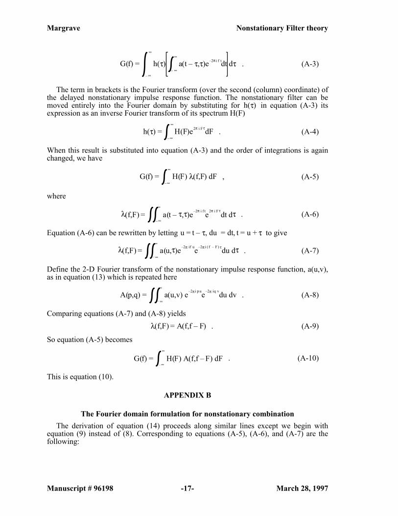
APPENDIX A

The Fourier domain formulation for nonstationary convolution Equation (8) is repeated here as

g(t) = a(t – τ,τ) h(τ) dτ– ∞

∞

. (A-1)

The spectrum, G(f), of g(t) is computed by the forward Fourier transform of equation (A-1)

G(f) = g(t)e–2π i f tdt– ∞

∞

= a(t – τ,τ)h(τ)dτ– ∞

∞

e–2π i f tdt– ∞

∞

. (A-2)

The next step is to reverse the order of integration in equation (A-2). Strictly speaking, this requires some justification. For integrals with non-infinite limits, a double integral over a rectangular region can have its integration order interchanged provided only that the integrand is continuous (see any calculus text, for example Courant and John, 1974, (Vol. II page 398) ). In improper integrals such as the 2-D Fourier transform, more consideration is required. Korner (1988) gives the general conditions under which the order reversal may be justified (his theorem 48.8) and these amount to requiring that the integrand is continuous, that both one dimensional transforms of the absolute value of the integrand are continuous, and that the 2-D transform itself converges absolutely. Of course, if the integrand has only compact support, then the infinite limits may be replaced by finite ones and the conditions are relaxed. All of the theory in this paper assumes that these conditions have been met in one way or the other. (Note that similar integration reversals are required to prove the Fourier transform theorem and the convolution theorem. For example see Korner (1988) or Morse and Feshbach (1953) ). Therefore, reversing the order of integration in equation (A-2) gives



G(f) = h(τ) a(t – τ,τ)e–2π i f tdt– ∞

∞

dτ– ∞

∞

. (A-3)

The term in brackets is the Fourier transform (over the second (column) coordinate) of the delayed nonstationary impulse response function. The nonstationary filter can be moved entirely into the Fourier domain by substituting for h(τ) in equation (A-3) its expression as an inverse Fourier transform of its spectrum H(F)

h(τ) = H(F)e2π i FτdF– ∞

∞

. (A-4)

When this result is substituted into equation (A-3) and the order of integrations is again changed, we have

G(f) = H(F) λ(f,F) dF– ∞

∞

, (A-5)

where

λ(f,F) = a(t – τ,τ)e–2π i f te2π i Fτdt dτ– ∞

∞

. (A-6)

Equation (A-6) can be rewritten by letting u = t – τ, du = dt, t = u + τ to give

λ(f,F) = a(u,τ)e–2π if ue–2π i ( f – F ) τdu dτ

– ∞

∞

. (A-7)

Define the 2-D Fourier transform of the nonstationary impulse response function, a(u,v), as in equation (13) which is repeated here

A(p,q) = a(u,v) e–2π i p ue–2π iq vdu dv

– ∞

∞

. (A-8)

Comparing equations (A-7) and (A-8) yields λ(f,F) = A(f,f – F) . (A-9)

So equation (A-5) becomes

G(f) = H(F) A(f,f – F) dF– ∞

∞

. (A-10)

This is equation (10).

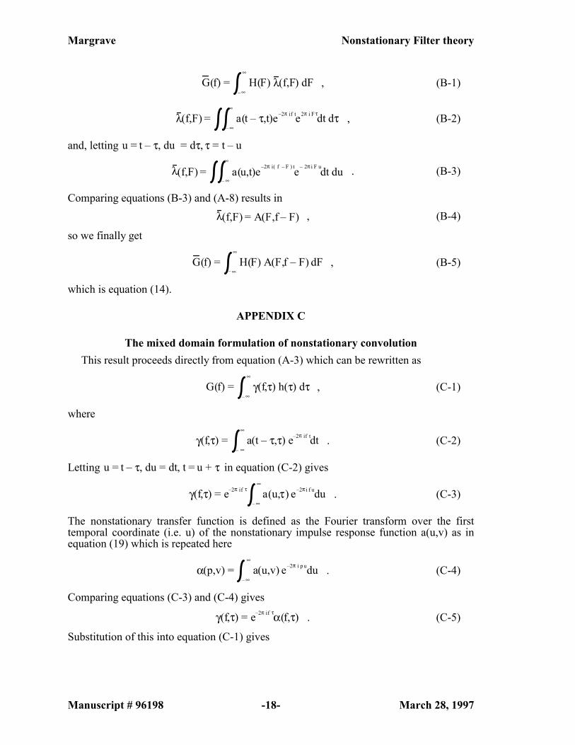
APPENDIX B

The Fourier domain formulation for nonstationary combination The derivation of equation (14) proceeds along similar lines except we begin with

equation (9) instead of (8). Corresponding to equations (A-5), (A-6), and (A-7) are the following:



G(f) = H(F) λ(f,F) dF– ∞

∞

, (B-1)

λ(f,F) = a(t – τ,t)e–2π if te2π i Fτdt dτ– ∞

∞

, (B-2)

and, letting u = t – τ, du = dτ, τ = t – u

λ(f,F) = a(u,t)e–2π i( f – F ) te– 2π i F udt du– ∞

∞

. (B-3)

Comparing equations (B-3) and (A-8) results in λ(f,F) = A(F,f – F) , (B-4)

so we finally get

G(f) = H(F) A(F,f – F) dF– ∞

∞

, (B-5)

which is equation (14).

APPENDIX C

The mixed domain formulation of nonstationary convolution This result proceeds directly from equation (A-3) which can be rewritten as

G(f) = γ(f,τ) h(τ) dτ– ∞

∞

, (C-1)

where

γ(f,τ) = a(t – τ,τ) e–2π if tdt– ∞

∞

. (C-2)

Letting u = t – τ, du = dt, t = u + τ in equation (C-2) gives

γ(f,τ) = e–2π if τ a(u,τ) e–2π i f udu– ∞

∞

. (C-3)

The nonstationary transfer function is defined as the Fourier transform over the first temporal coordinate (i.e. u) of the nonstationary impulse response function a(u,v) as in equation (19) which is repeated here

α(p,v) = a(u,v) e–2π i p udu– ∞

∞

. (C-4)

Comparing equations (C-3) and (C-4) gives

γ(f,τ) = e–2π if τα(f,τ) . (C-5)

Substitution of this into equation (C-1) gives



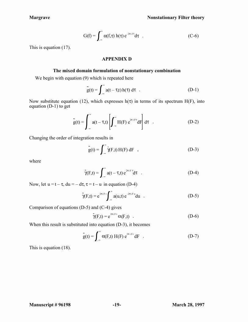
G(f) = α(f,τ) h(τ) e–2π i f τdτ– ∞

∞

. (C-6)


APPENDIX D

The mixed domain formulation of nonstationary combination We begin with equation (9) which is repeated here

g(t) = a(t – τ,t) h(τ) dτ– ∞

∞

. (D-1)

Now substitute equation (12), which expresses h(τ) in terms of its spectrum H(F), into equation (D-1) to get

g(t) = a(t – τ,t) H(F) e2π i FτdF– ∞

∞

dτ– ∞

∞

. (D-2)

Changing the order of integration results in

g(t) = γ(F,t) H(F) dF– ∞

∞

, (D-3)

where

γ(F,t) = a(t – τ,t) e2π i F τdτ– ∞

∞

. (D-4)

Now, let u = t – τ, du = – dτ, τ = t – u in equation (D-4)

γ(F,t) = e2π i F t a(u,t) e–2π i F udu– ∞

∞

. (D-5)

Comparison of equations (D-5) and (C-4) gives

γ(F,t) = e2π i F t α(F,t) . (D-6)

When this result is substituted into equation (D-3), it becomes

g(t) = α(F,t) H(F) e2π i F t dF– ∞

∞

. (D-7)




FIGURE CAPTIONS FIG. 1. An illustration of stationary convolution as a time domain matrix operation.

Beneath each matrix or vector is the function notation of their continuous analogues. (a) is the stationary convolution matrix for a particular minimum phase bandpass filter. The matrix displays Toeplitz symmetry meaning that each column contains the filter impulse response, each row contain the time reverse of the impulse response, and any diagonal is constant. (b) is a reflectivity series in time to which the convolution matrix is applied. (c) is the output stationary seismogram.

FIG. 2. An illustration of nonstationary convolution as a time domain matrix operation which is the discrete equivalent to equation (8). (a) is the nonstationary convolution matrix for a particular forward Q filter bandlimited by the stationary waveform of Figure 1. Each column contains the convolution of the minimum phase waveform of Figure 1 and the minimum phase impulse response of a constant Q medium for a traveltime equal to the column time. (b) is a reflectivity series in time to which the convolution matrix is applied. (c) is the output constant Q seismogram.

FIG. 3. The impulse response matrices, which are the discrete equivalents of a(u,v), for (a) Figure 1 and (b) Figure 2. (a) is a stationary minimum phase bandpass filter and is therefore invariant with v. (b) is a minimum phase constant Q impulse response matrix (bandlimited by the waveform in (a)) that varies strongly with v in both amplitude and phase. Note that the vertical timing scales are considerably enlarged relative to Figures 1 and 2. The convolution matrices in Figures 1 and 2 are formed by delaying each column of (a) and (b) respectively such that the time zero is on the main diagonal.

FIG. 4. The application of the stationary filter of Figure 1 in the Fourier domain using the matrix formalism equivalent to equations (10) and (13). (a) is the frequency connection matrix (only the amplitude spectrum is shown), (b) is the complex spectrum of the input trace, and (c) is the complex spectrum of the output trace. The matrix (a) is purely diagonal which is a direct consequence of the fact that the impulse response matrix (Figure 3 (a)) is stationary. The spectra (b) and (c) are each related to their time domain equivalents in Figure (1) by an ordinary inverse Fourier transform. (In this and other figures, complex spectra are plotted by interleaving real and imaginary samples. Thus the real part of the spectrum is the odd numbered samples and the imaginary part is the even numbered samples.)

FIG. 5. The application of the nonstationary forward Q filter of Figure 2 in the Fourier domain using the formalism of equations (10) and (13). (a) is the frequency connection matrix (only the amplitude spectrum is shown), (b) is the complex spectrum of the input trace, and (c) is the complex spectrum of the output trace. (a) is computed from the 2-D Fourier transform of the impulse response matrix (Figure 3 (b)) and the off diagonal energy arises because the later matrix is nonstationary. The spectra (b) and (c) are each related to their time domain equivalents in Figure (2) by an ordinary inverse Fourier transform.

FIG. 6. Nonstationary convolution is represented in the (f,τ) domain for the stationary case of Figures 1 and 4. The computation of the matrix equation equivalent to equation (17) is depicted except for a Fourier matrix representing exp(-2πifτ). (a) is the "nonstationary" transfer matrix (amplitude spectrum only) which is computed by Fourier transforming the columns of the matrix in Figure 3a, (b) is the input reflectivity series in the time domain, and (c) is the Fourier spectrum of the desired result.

FIG. 7. Nonstationary convolution is represented in the (f,τ) domain for the nonstationary case of Figures 2 and 5. The computation of the matrix equation equivalent to equation (17) is depicted except for a Fourier matrix representing exp(-2πifτ). (a) is the



nonstationary transfer matrix (amplitude spectrum only) which is computed by Fourier transforming the columns of the matrix in Figure 3b, (b) is the input reflectivity series in the time domain, and (c) is the Fourier spectrum of the desired result.

FIG. 8. An illustration of the construction of g(t) by nonstationary combination as a slice through the family of stationary filtered results gj(t). Each gj(t) may be considered as a conventionally filtered trace while the index j runs across all possible filters in the nonstationary transfer function.

FIG. 9. The relationship between the various forms of nonstationary filter specification: the nonstationary impulse response function, a(u,v), the nonstationary transfer function, a(p,v), and the frequency connection function, A(p,q). Arrows to the right represent forward Fourier transforms while those to the left are inverse Fourier transforms. The four shorter arrows are 1-D transforms while the two longer arrows are 2-D transforms.

FIG. 10. A mixed domain design for a time variant minimum phase bandpass filter. (a) is the amplitude spectrum which varies from about 10-80 Hz at time 0 to 10-40 Hz at time 1.0 seconds. It is stationary from 1.0 to 2.0 seconds. (b) is the minimum phase spectrum. A column of (b) is computed as the Hilbert transform of the logarithm of a column of (a). (Compare to Figure 7).

FIG. 11. (a) is the frequency connection matrix, the discrete equivalent to A(f,f-F), (amplitude spectrum only) for the minimum phase filter of Figure 10. (b) is similar except that a zero phase spectrum was used. When either matrix is used to multiply the spectrum of a seismic trace, the result is the spectrum of the time variant filtered trace. (Compare to Figure 5).

FIG. 12. (a) is the time domain nonstationary convolution matrix for the minimum phase filter design of Figure 10. (b) is similar except that a zero phase spectrum was used. When either matrix multiplies a seismic trace, the result is a time variant filtered trace. (Compare to Figure 2).

FIG. 13. Several results of the application of time variant filters to an input "comb function" (a) are shown. The minimum phase result (b) used the filter design of Figure 10. The zero phase result (c) used the amplitude spectrum from Figure 10 with a zero phase spectrum. The linear phase result (d) used the same amplitude spectrum with a phase shift that varied linearly from 0 degrees at time zero to 90 degrees at 1 second.

FIG. 14. A time variant amplitude spectrum computed from one of the filtered traces in Figure 13. It was computed using a "short time Fourier transform" with a .3 second window and 95% overlap between windows. The bold vertical line marks 1.0 seconds. Comparison with Figure 10a shows that the amplitude spectrum design was achieved.

FIG. 15. A comparison of nonstationary convolution (equation 8) and nonstationary combination (equation 9) as applied to the comb function of Figure 13. (a) and (b) applied the amplitude spectrum of Figure 10a with a zero phase spectrum while (d) and (e) applied the full minimum phase design in Figure 10. Though similar, the processes differ more for the minimum phase filter because it is less stationary. Note the contrasting wraparound effects for the zero phase case.

FIG. 16. A comparison of nonstationary convolution (equation 8) and combination (equation 9) for an abruptly changing filter. (a) is the amplitude spectrum used (the discontinuity is at .5 seconds), (b) is a reflectivity sequence to be filtered, (c) is a minimum phase convolution of (a) with (b), (d) is a minimum phase combination, and (e) is the difference of (d) from (c).

theory of nonstationary linear filtering in the …-1- march 28, 1997 theory of nonstationary linear...

Documents