theory and practice of quantitative microbial risk...
TRANSCRIPT

Theory and Practice of Quantitative
Microbial Risk Assessment: An Introduction
Joan B. Rose
Patrick L. Gurian
Charles N. Haas
Joe Eisenberg
Jim Koopman
Mark Nicas
Tomoyuki Shibata
Mark H. Weir
Revision Date: June 28, 2013

2
Authors
Joan B Rose Michigan State University
Charles N Haas Drexel University
Patrick L Gurian Drexel University
Mark H Weir Michigan State University
Jim Koopman University of Michigan
Joe Eisenberg University of Michigan
Mark Nicas University of California Berkeley
Tomoyuki Shibata University of Miami
Acknowledgements:
This manual is a result of efforts by Center for Advancing Microbial Risk Assessment
(CAMRA) scientists as they have been involved in the development of QMRA and
educational institutes. This was partially funded by EPA and DHLS.

3
Table of contents
CHAPTER 1: QUANTITATIVE MICROBIAL RISK ASSESSMENT FRAMEWORKS ................. 6
JOAN B. ROSE......................................................................................................................................... 6
GOAL ..................................................................................................................................................... 6 DEFINITIONS ........................................................................................................................................... 6 RISK ....................................................................................................................................................... 7 MICROORGANISMS AND DISEASE RISKS .................................................................................................. 9 QUANTITATIVE RISK ASSESSMENT FRAMEWORKS ................................................................................. 10 QMRA: QUANTITATIVE MICROBIAL RISK ASSESSMENT ....................................................................... 11 EXAMPLE OF DOSE AND RESPONSE FOR CHOLERA................................................................................. 15 RISK MANAGEMENT AND QMRA ......................................................................................................... 18 EXAMPLE 1.1 ........................................................................................................................................ 20 REFERENCES AND FURTHER READING ................................................................................................... 21
CHAPTER 2: MEASURING MICROBES .......................................................................................... 22
JOAN B. ROSE....................................................................................................................................... 22
GOAL .................................................................................................................................................. 22 TYPES OF MICROBES AND TYPES OF UNITS ........................................................................................... 22 GENETIC DETECTION AND CHARACTERIZATION .................................................................................... 23 SAMPLING AND METHOD DEVELOPMENT ISSUES ................................................................................... 24 EXAMPLE 2.1 EVALUATION OF SCREENING TESTS FOR SPECIFICITY AND SENSITIVITY ............................ 25 REFERENCE .......................................................................................................................................... 27 EXAMPLE 2.2 PRIMER DESIGN AND GENBANK EXERCISE ........................................................................ 28
CHAPTER 3: STATISTICS AND UNCERTAINTY .......................................................................... 32
PATRICK L. GURIAN .......................................................................................................................... 32
GOAL ................................................................................................................................................... 32 PROBABILITY........................................................................................................................................ 32 EXAMPLE 3.1 FINDING THE CDF OF A NORMAL DISTRIBUTION ............................................................... 35 PARAMETER ESTIMATES ....................................................................................................................... 35 VARIABILITY AND UNCERTAINTY ......................................................................................................... 37 EXAMPLE 3.2 MAXIMUM LIKELIHOOD ESTIMATION .............................................................................. 38 BOOTSTRAPPING ................................................................................................................................... 40 EXAMPLE 3.3 BOOTSTRAP UNCERTAINTY ANALYSIS ............................................................................. 41 REFERENCES AND FURTHER READING ................................................................................................... 41
CHAPTER 4: ANIMAL AND HUMAN STUDIES FOR DOSE-RESPONSE ................................... 42
CHARLES N. HAAS .............................................................................................................................. 42
GOAL ................................................................................................................................................... 42 ANALYTICAL HUMAN STUDIES ............................................................................................................. 42
Examples of Analytical Studies ........................................................................................................ 43 Classic Cohort Study ............................................................................................................................................43 Classic Case Control Study ..................................................................................................................................43 Cohort Study with Quantitative Exposure Metric ...............................................................................................44
EXPERIMENTAL HUMAN AND ANIMAL STUDIES .................................................................................... 45 Experimental Human Study Example ............................................................................................... 45
REFERENCES ........................................................................................................................................ 47
CHAPTER 5: DOSE-RESPONSE ........................................................................................................ 48
CHARLES N. HAAS .............................................................................................................................. 48
GOAL ................................................................................................................................................... 48

4
PLAUSIBLE DOSE RESPONSE MODELS ................................................................................................... 48 FITTING AVAILABLE DATA ................................................................................................................... 50
Types of Data Sets ........................................................................................................................... 50 Best Fit Estimation .......................................................................................................................... 50
EXAMPLE 5.1 ........................................................................................................................................ 51 Goodness of Fit Determinations ...................................................................................................... 53
EXAMPLE 5.2 ........................................................................................................................................ 54 Comparison of Nested Models ......................................................................................................... 54 Confidence Intervals and Regions ................................................................................................... 55
REFERENCES ........................................................................................................................................ 57
CHAPTER 6: INTRODUCTION TO EXPOSURE ASSESSMENT .................................................. 58
TOMOYUKI SHIBATA ........................................................................................................................ 58
GOAL ................................................................................................................................................... 58 CHANGES IN MICROBIAL CONCENTRATIONS ........................................................................................... 58 % VS. LOG REDUCTION ......................................................................................................................... 59 INACTIVATION RATE............................................................................................................................. 60 EXAMPLE 6.1 RECOVERY AND INACTIVATION ON FOMITES .................................................................... 60 EXPOSURE DOSE ................................................................................................................................... 65 EXPOSURE PATHWAYS: WATER, AIR, SOIL, AND FOOD.......................................................................... 65 EXAMPLE 6.2 INGESTION OF WATER .................................................................................................... 65 EXPOSURE PATHWAY: FOMITES ............................................................................................................ 69 EXAMPLE 6.4 FOMITE EXPOSURE .......................................................................................................... 70 RISK CHARACTERIZATION AND MANAGEMENT ..................................................................................... 72 RETROSPECTIVE ASSESSMENT .............................................................................................................. 72 EXAMPLE 6.5 RETROSPECTIVE EXPOSURE ASSESSMENT ........................................................................ 72 EXPOSURE REDUCTION ......................................................................................................................... 73 EXAMPLE 6.6 HAND WASHING ............................................................................................................. 73 REFERENCES ........................................................................................................................................ 78
CHAPTER 7: MONTE CARLO AND CRYSTAL BALL® ................................................................. 79
MARK H. WEIR .................................................................................................................................... 79
GOAL .................................................................................................................................................. 79 BACKGROUND ................................................................................................................................. 79 EXAMPLE 7.1 GENERATION OF ROULETTE NUMBERS EXAMPLE.............................................................. 80 MONTE CARLO SIMULATIONS ............................................................................................................... 80 USING CRYSTAL BALL FOR THE MONTE CARLO METHOD...................................................................... 81 EXAMPLE 7.2 PROBABILITY OF INFECTED INDIVIDUAL BEING SEATED IN YOUR ROW. .............................. 84 EXAMPLE 7.3 FITTING A PROBABILITY DISTRIBUTION IN CRYSTAL BALL® ............................................. 85 EXAMPLE 7.4 MAKING A CUSTOM DISTRIBUTION IN CRYSTAL BALL® ................................................... 87 EXAMPLE7.5 DEFINING THE DOSE RESPONSE MODEL FOR TB AS A FORECAST IN CRYSTAL BALL® .......... 88 RISK TO AN AIRLINE PASSENGER OF BEING INFECTED WITH TB ............................................................... 94
CHAPTER 8: FATE AND TRANSPORT MODELS: INDOOR AIR/FOMITES ............................. 97
MARK NICAS ........................................................................................................................................ 97
GOAL .................................................................................................................................................. 97 DEFINITIONS .................................................................................................................................... 97 EXAMPLE 8.1 SCENARIO AND ANALYTICAL SOLUTION ...................................................................... 98 EXAMPLE 8.2 THE MARKOV CHAIN METHOD .................................................................................. 100 EXAMPLE 8.3 AN AIRBORNE PATHOGEN SCENARIO .......................................................................... 103 ADDITIONAL IDEAS ON MODELING PARTICLE FATE AND TRANSPORT .................................................. 110 EXAMPLE 8.4 FATE AND TRANSPORT ON SURFACES (FOMITES) ....................................................... 111
Sample MATLAB code for running the surface-to-hand-to-face transfer model ........................................... 120
CHAPTER 9: INTRODUCTION TO DETERMINISTIC DYNAMIC DISEASE MODELING .... 122

5
JIM KOOPMAN .................................................................................................................................. 122
ANALYZING DYNAMICS RATHER THAN RISKS....................................................................................... 122 TYPES OF MODELS .............................................................................................................................. 123
Goals of infection transmission modeling ...................................................................................... 125
CHAPTER 10: ENVIRONMENTAL INFECTION TRANSMISSION SYSTEM MODELS ......... 128
JOSEPH EISENBERG......................................................................................................................... 128
GOAL ................................................................................................................................................. 128 OVERVIEW OF MATLAB .................................................................................................................... 128 BRIEF BACKGROUND ON SOME USEFUL MATLAB FUNCTIONS ............................................................ 128 MATLAB SCRIPTS (M-FILES) ............................................................................................................ 129 TRANSMISSION MODELING IN MATLAB ............................................................................................. 130 EXPLORING INTERVENTION OPTIONS USING AN ENVIRONMENTAL INFECTION TRANSMISSION SYSTEM
(EITS) MODEL ................................................................................................................................... 131
CHAPTER 11: RISK PERCEPTION, RISK COMMUNICATION, AND RISK MANAGEMENT
............................................................................................................................................................... 136
PATRICK L. GURIAN ........................................................................................................................ 136
GOAL ................................................................................................................................................. 136 RISK PERCEPTION ............................................................................................................................... 136 RISK COMMUNICATION ....................................................................................................................... 139 RISK MANAGEMENT ........................................................................................................................... 141 ACKNOWLEDGEMENT ......................................................................................................................... 144 REFERENCES/SUGGESTED READING .................................................................................................... 144
APPENDIX A: LIST OF ACRONYMS .............................................................................................. 145

6
Chapter 1: Quantitative Microbial Risk Assessment Frameworks
Joan B. Rose
GOAL
This chapter will provide an overview of the various frameworks that have been used for
risk assessment (RA) and particularly for quantitative microbial risk assessment (QMRA).
A brief history of the developments and advancements will assist in understanding the
terminology used to describe MRA and the definitions which have evolved from other
disciplines. The framework provides a structure for taking data from a variety of sources
(including information from models) and integrating them in such a way where one could
begin to articulate and quantify a complex problem.
DEFINITIONS
Microbial risk assessment is an approach to address microorganisms that cause harm
most often in humans which is described by the types of diseases and symptoms
associated with the infections. There are many terms used by the medical community,
public health professionals, scientists and others such as journalists, to describe disease
status. These are often confusing. Thus one goal is to harmonize the terms with a clear
understanding of the meanings to improve communications. Many terms are used
including Contagion, Disease, Dose, Exposure and Infection and the definitions may
differ within the QMRA community and the medical community.
Contagion: is the ability for microorganisms to be transferred from one infected
individual to another, which means that live organisms are excreted by the infected
individual in some fashion and are able to be passed onto another susceptible individual.
In the modeling world, one can estimate the probability of transmission of the
microorganism from the one person who is infected to a susceptible individual based on
exposure scenarios and the characteristics of the microorganism, the excretion rates and
the contact rate, thus estimates of very low risks can be made: 1 in million (10 -6 ) or 1 in
10 million (10 -7 ), or 1 in a billion (10 -9 ); in the real-world and medical world very
high levels of disease transmission can be evaluated through epidemiological
investigations (1 in 10; 1/100) but generally this is addressed as YES or NO without
quantification of probability. Epidemiology may describe estimated attack rates
(associated with the numbers of infected in the numerator/number exposed in the
denominator).
Disease: is the impairment of the persons health status or impairment of some function;
in the medical world often used to synonymously and confused with infection.

7
Dose: is the actual number of pathogenic microorganisms which are ingested, breathed
in, or contacted.
Exposure: in the risk assessment modeling world this means that the individual actually
received some dose; HOWEVER in the real-world situation it means that the individual
was exposed to the source of the contaminant (not knowing if they really received a
dose or not, e.g. exposed to the swimming pool); in the medical world one may look to
see if there is evidence of exposure from some clinical test (antibody response or
identification of a biomarker or for the biological agent itself).
Infection: describes that a microorganism is able to initiate and replicate in the host.
This is measurable in experiments by antibody response or identification of the biological
agent at the site of replication or via excretion rates.
RISK
Risk in most people’s minds is related to some type of harmful event and in fact the
assessment of that risk is done a priori in order to determine a way to avoid or reduce the
chance of harm occurring (Table 1.1). Thus in the simplest terms this is defined as:
risk =exposure* hazard (1.1)
But in assessing this it is described as a probability. So what is the chance of exposure
to some hazard and if exposed what is the consequence (or how severe is the harm).
Time is an element of risk as well, because how often is one exposed for how long, as
well as who is exposed will influence the outcome. Thus risk is the likelihood of
(identified) hazards causing harm in exposed populations in a specified time frame
including the severity of the consequences. Some hazards are known and better described
than others and may be natural hazards or human induced. One can think of many
examples of risks and hazards and ways that we assess these and reduce them. Some are
individual choices and some are more societal. Some are greater “risks” for special
groups of individuals, like children. Some risks are accepted at certain rates or
probabilities (e.g. 1/100 chance) because of associated benefits associated with the
activity or because there are ways to help mitigate the problem after the fact.

8
The field of risk analysis is described by discussing generally three areas:
Risk Assessment: The qualitative or quantitative characterization and estimation of
potential adverse health effects associated with exposure of individuals or populations to
hazards (materials or situations, physical, chemical and or microbial agents.)
Risk management: The process for controlling risks, weighing alternatives, selecting
appropriate action, taking into account risk assessment, values, engineering, economics,
legal and political issues.
Risk communication: The communication of risks to and between managers,
stakeholders, public officials, and the public, includes public perception and ability to
exchange scientific information.
Table 1.1 discusses some common risks and concurrent management strategies.
Table 1.1 Risk reduction strategies
Examples of risks Risk reduction strategies
Riding in a car and having
an accident
Drive the speed limit; wear seat belts; use child seats.
Improve safety features of cars.
Improve roads and key interchanges etc.
Crossing the street and
being hit by a car
Use cross-walks, look both ways, install a light or stop
sign; install pedestrian overpass.
Second hand smoking and
cancer
Ban smoking in public places.
Bridges collapsing Have inspections, maintenance and repair programs
Hurricanes, infrastructure
damage, life lost, illness,
stress.
Provide Early warning. Avoid building in susceptible
areas. Develop disaster preparedness plans.
Medicines and side effects Have appropriate testing prior to market. Take only
medicines prescribed. Be sure there is consumer
awareness of potential side effects.

9
MICROORGANISMS AND DISEASE RISKS
Advances in medicine and microbiology have formed the basis of our understanding of
disease and infectious disease risks (Beck, 2004). Ancient medicine addressed diagnosis
of illness via the description of symptoms and the first recorded terms and descriptions
of epidemics (large numbers of individuals ill at the same place during a similar time
period) took place in ca. 3180 B.C. in Egypt. Early diseases were eluded to as
“epidemic fevers” the term written in a papyrus ca. 1500 B.C. discovered in a tomb in
Thebes, Egypt. Early in the history of medicine it was proposed that bad air, putrid
waters, and crowding were all associated with disease and it was recognized that these
maladies were contagious (spread from one ill person to another). “Plagues” were
described and in particular associated with the decimation of the Greek Army near the
end of the Trojan War (ca. 1190 B.C.) with massive epidemics described in Roman
history in 790, 710 and 640 B.C. (Sherman, 2006) One of the best described plagues
occurred in Athens in 430 BC. What appeared to be dysentery epidemics (enteric
fevers) were described in 580 AD. However, it was not until the 1500-1700s that
advances first in microbiology lead the way for discoveries in medicine which solidified
the idea of bacteria and led to the “germ theory”, pathogen discovery and the
understanding of disease transmission.
The germ theory had been suggested in 1546 by Girolomo Fracastoro (publishing De
contagione) and while infectious diseases were being described it was not until the
microscope was invented in 1590 and refined in 1668 that parasites and then bacteria
were first seen in 1676 and then fully described in 1773 by Otto Frederik Muller (likely
describing Vibrio ). The “germ theory” was further solidified in 1840 and nine years
later John Snow was able to show that Cholera was transmitted through water (1849).
Yet the translation of this knowledge to other organisms was slow. It was not until 1856
that it was suggested that Typhoid fever was spread by feces and by then a scientific
method to identify “contagious agents” using Robert Koch theories (1876) moved the
study of cause-and-effect forward. A significant microbiological advancement was the
invention of the culture technique using salts and yeast in 1872 and then a plating
technique in 1881 using gelatin. Robert Koch not only addressed these plating
techniques, but brought into microbiological practice the use of sterilization (what is
now known as the autoclave). Gram stains came along and the Escherichia coli was
isolated from feces (1884 and 1885, respectively) but it took 25 more years for the
“coliform” to make its way into water sanitation and health practices to address fecal
contamination (1910). In that same time period (1884), Koch isolated a pure culture of
Vibrio and Georg Gaffky isolated the typhoid bacillus.
Epidemiology: is the study of the spread of disease in populations and is a scientific
method for addressing microbial risks. Dr. John Snow is credited as the father of
epidemiology. A major turning point in protection of community health and prevention
of epidemics came in the mid-19th century. During an epidemic of cholera which had
broken out in India in 1846, John Snow observed that cholera was transmitted through
drinking water. He was then able to test his theory using one of the first engineering

10
controls, by simply removing handle from a water pump, which he suspected as the cause
of the outbreak in a district in London.
Thus it was the convergence of engineering, medicine, epidemiology, and public health
that led to an improved understanding of the risks of infectious microbial agents .
Pathogens: are those microorganisms that cause illness and disease) and infection
transmission models for describing how disease spreads in populations were developed to
mathematically describe the movement of pathogens in communities (susceptibles) (See
Chapters 9 and 10). In addition, in the early development of vaccines and establishment
of Koch’s postulates for example for new pathogens like Giardia, human dosing studies
were undertaken, where by different groups of volunteers were given different doses
(from the 1930s to 1990s) and the disease or infection outcome was monitored, thus
dose-response data were experimentally obtained. Currently strict ethics rules apply to
any type of study using humans for these types of dose-response studies.
Epidemiological methods continued to examine disease risks and during outbreaks
(more than 1 person ill from a common exposure at a similar time; e.g. foodborne,
waterborne, nursing home; daycare outbreaks) attack rates (ratio of those ill/those
exposed) would be related to some exposure and dose to attempt to show a relationship
(e.g. those individuals that had 3 servings of potato salad had higher attack rates than
those who had 1 serving). In prospective studies for example for swimming in polluted
waters, Stevenson in 1957 determined that there was a relationship between the amount
of pollution as measured by fecal indicator bacteria in the water and the disease rate in
swimmers. Thus this also established dose-response data which could be
mathematically fitted and modeled. However, the main difference is that this
approach does not address the group of possible pathogens.
QUANTITATIVE RISK ASSESSMENT FRAMEWORKS
Formal quantitative risk frameworks were first developed and described as nations
industrialized, and in the US, in particular the role of chemicals in the environment
causing harm such as DDT, PCBs, and lead in the 1960s created a need to assess
environmental pollution risks and approaches for their control. The National Academy of
Sciences (NAS) developed a risk framework that was published in the famous “Red
Book” that would go on to form the basis of scientific assessment and regulatory
strategies for environmental pollutants (Table 1.2). This was an approach to
mathematically (through modeling using dose-response relationships) estimate the
probability of an adverse outcome.

11
Table 1.2 NAS framework for quantitative risk assessment adapted for QMRA
Four steps for QRA Types of information used for pathogens
Hazard Identification Description of the microorganisms and disease end-
points, severity and death rates
Dose-Response Human feeding studies, clinical studies, less
virulent microbes, vaccines and healthy adults
Exposure Monitoring data, indicators and modeling used to
address exposure. Epidemiological data used to link
specific exposures to health outcomes.
Risk Characterization Description of the magnitude of the risk, the
uncertainty and variability.
These QRAs were then used for management decision and addressing other issues
including risk communication, which formed the larger arena of “Risk Analysis”.
Following the new framework suggested by the recent report “Science and Decisions:
Advancing Risk Assessment” from the National Academy of Sciences (NRC 2008), the
process now integrates the problem identification and risk management strategies to the
risk assessment.
QMRA: QUANTITATIVE MICROBIAL RISK ASSESSMENT
It was recognized early on that the risks and the assessment of the risks associated with
microorganisms (pathogens) were very different from chemicals. Epidemiological
methods had been used but were limited by sensitivity (in most cases large numbers of
people were needed in any given study and the methods could usually only examine risks
on the order of 1/1000). Epidemiological studies were poor at addressing quantitative
exposures. Microbes also can change dramatically in concentrations (grow or die-off),
the methods for their destruction or control are in place (disinfection and vaccinations)
and they are contagious for the most part, so that one exposure can lead to a cascading
effect. Pathogens change genetically (e.g. E. coli and emergence of pathogenic E. coli)
and there are new pathogens being discovered (e.g. Bird Influenza). Some pathogens are
transmitted by many routes (e.g. air, food, water, hands) and some are restricted to certain
modes of transmission (e.g. Dengue virus being mosquito-borne; tuberculosis, respiratory
person-to-person transmission).
The four steps for a QMRA included the following:
• Hazard Identification – To describe acute and chronic human health effects;
severity, sensitive populations, immunological response for specific pathogens.
• Dose-Response – To characterize the relationship between various doses
administered and subsequent probability of infection or health effects; human data
sets are available.

12
• Exposure Assessment – To determine the size and nature of the population
exposed and the route, amount, and duration of exposure. Temporal and spatial
exposure with changes in microbial populations are a concern.
• Risk Characterization – To integrate the information from exposure, dose
response, and health steps to estimate magnitude of health risks. Monte Carlo
analysis is used to give distribution of risks and infection transmission models are
used to address community risks. Uncertainty and variability are addressed.
The International Life Sciences Institute (ILSI), working with the US Environmental
Protection Agency (US EPA), developed a framework that was more specific to
addressing microbial risks and moved toward new concepts of risk assessment where by
the problem and management were integral to the risk process (Figure 1.1).
The goal for QMRA is to start with a problem formulation and gather information on the
hazards, dose-response models and tie that to the possible exposures over time, in order
to address risk characterization not only to individuals but to communities and
populations..
For the hazard identification we need to describe in more detail the microbe, and
quantitatively the disease symptoms and severity, particularly in sensitive populations,
like the elderly or children. In order to do so more efforts are needed for QMRA to:
Engage the medical community to obtain data
Address epidemiological data
Mandate better Outbreak investigations
Undertake Pathogen Discovery (application of new technologies for genetic characterization)

13
RISK CHARACTERIZATION
CHARACTERIZATION
of Exposure of HumanHealth Effects
ANALYSIS
PROBLEM FORMULATION
RISK MANAGEMENT OPTIONS
Exposure Profile
Host Pathogen Profile
ANALYSIS PHASE
Exposure Analysis
Pathogen Occurrence
Health Effects
Dose-Response
Exposure Profile
Host Pathogen Profile
ANALYSIS PHASE
Exposure Analysis
Pathogen Occurrence
(detection/survival
and spread)
Health Effects
Disease
Severity
Secondary spread
Dose-Response
Figure 1.1 ILSI QMRA framework

14
Bacteria, parasites and viruses may cause a wide range of acute and chronic diseases as
well as death (Table 1.3).
Table 1.3 Some microorganisms and outcomes of exposures
Microorganisms Acute disease Chronic disease
Campylobacter Diarrhea Guillain-Barré syndrome
E. coli O15:H7 Diarrhea Hemolytic uremic
syndrome
Helicobacter Gastritis Ulcers and stomach cancer
Salmonella,
Shigella, Yersinia Diarrhea Reactive arthritis
Coxsackievirus B
Adenoviruses
Encephalitis, aseptic
Meningitis, diarrhea,
respiratory disease
Diabetes
Myocarditis
Obesity
Giardia Diarrhea
Failure to thrive, lactose
intolerance, chronic joint
pain
Toxoplasma Newborn syndrome,
hearing and visual loss
Mental retardation,
dementia, seizures
There are over 70 dose-response data sets modeled to date. These are stored on the
QMRAwki:
[http://qmrawiki.msu.edu/index.php?title=Quantitative_Microbial_Risk_Assessment_(Q
MRA)_Wiki]
However some of the issues that remain include:
Human data sets used healthy volunteers
Vaccine strains or less virulent organisms were used.
Low doses often not evaluated
Doses measured with mainly cultivation methods for bacteria and viruses
(colony or plaque forming units CFU) for parasites counted under the
microscope. New methods will need to address molecular measurements.
Responses need to be related which include excretion in the feces, antibody response and illness.
Animal models are needed to address human subjects use and limitations in the future, including multiple low doses.

15
EXAMPLE OF DOSE AND RESPONSE FOR CHOLERA
Probability of Infection of Vibrio cholera associated with ingestion of 1, 10, 100 and
1000 viable bacteria (beta-poison model Haas and Rose: α=0.5487 and N50 =2.13x10⁴)
can be modeled based on the specific Probability of Infection Models developed for a
specific strain of Vibrio SEE Chapters 4 and 5.
Pi=
1 1d
N5021/
1
(1.2)
0.00%
0.01%
0.10%
1.00%
10.00%
100.00%
1.00E+00 1.00E+01 100 1.00E+03
Figure 1.2. Probabilistic risk of Cholera infection
Exposure
Exposure assessment is the translation of the environmental concentrations found (eg in
water or food) to describing the variability of the pathogen dose. The levels of pathogens
in the various doses that can occur over time and space are complex and defining the dose
is one of the most important aspects and most difficult for providing input to risk
characterization.
There is a need for better monitoring data and better environmental transport
models in air, water, food, soil, on surfaces etc.
Dose numbers of bacteria ingested
RISK
1/100=1% from single exposure
Risk (Pi)

16
In particular the ability to model survival/persistence of pathogens in the environment will be needed.
There will need to be new and better methods used which can address the hazard
as well as the exposure (e.g. qPCR, see Chapter 2 Measuring Microbes) for better
assessment of non-cultivatible but important viruses and bacteria.
For risk characterization probability of infection, morbidity and mortality can be
evaluated (Figure 1.3) by multiply the morbidty by the Probability of infection and that
by the mortality. Good medical data are needed and numerators and denominators for
mobidity and mortality rates need to be well defined.
Figure 1.3 Infection Diagram

17
In some cases a new paradigm is used that merges the infection transmission models
which come from tbe epidemiology field with the environment exposures and dose-
response functions (Figure 1.4) (See chapter 9).
Interaction between Disease Transmission
and the Environment
Green boxes: Epidemiological State
Red box: Pathogen Source / Sink
Solid Line: Movement of Population
Dotted Line: Movement of Pathogen
ExposedCarrier
Post - InfectionPost - Infection
Susceptible
DiseasedDiseased
Pathogen Fate
And
Transport
Pathogen Fate
And
Transport
ß
Exposure
Assessment:
Exposure
Assessment:
Psym
External
Environment
person - person
person-environment
Dose-response:
Dose-response:
Figure 1.4 Interaction between disease transmission and the environment
18
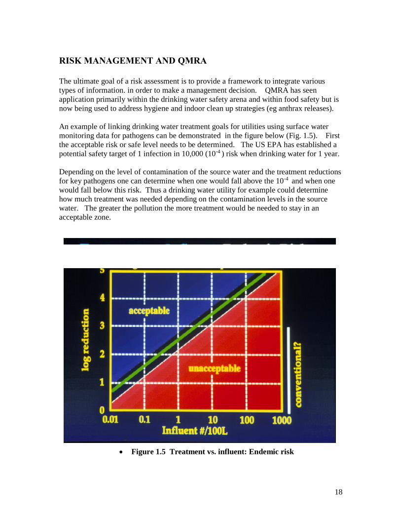
RISK MANAGEMENT AND QMRA
The ultimate goal of a risk assessment is to provide a framework to integrate various
types of information. in order to make a management decision. QMRA has seen
application primarily within the drinking water safety arena and within food safety but is
now being used to address hygiene and indoor clean up strategies (eg anthrax releases).
An example of linking drinking water treatment goals for utilities using surface water
monitoring data for pathogens can be demonstrated in the figure below (Fig. 1.5). First
the acceptable risk or safe level needs to be determined. The US EPA has established a
potential safety target of 1 infection in 10,000 (10-4 ) risk when drinking water for 1 year.
Depending on the level of contamination of the source water and the treatment reductions
for key pathogens one can determine when one would fall above the 10-4 and when one
would fall below this risk. Thus a drinking water utility for example could determine
how much treatment was needed depending on the contamination levels in the source
water. The greater the pollution the more treatment would be needed to stay in an
acceptable zone.
Figure 1.5 Treatment vs. influent: Endemic risk

19

20
Example 1.1 Framing the QMRA
GOALS: To understand the development of the various types of frameworks that could
be used to address QMRA and to identify the data sets needed to undertake a microbial
risk assessment.
Step 1. Develop a Problem Formulation on some microbial risk
a. Group A) TB and air travel, B) Norovirus outbreak, C) Extreme event;
Flooding; and D: Beach contamination (sewage spill) and cleanup.
b. Articulate the problem, name the stakeholders involved, and address the
perception of the problem.
Discussion
Who are the people involved in the problem either helping cause it or fix it or the
victims of it? How big is the problem? Geographically (is it a local problem or is
it national) Why? How serious is the problem?
Step 2. Hazard Identification: List and Describe
a. The microbial hazards
b. The transmission route (or routes)
c. The populations involved
d. The health outcomes
e. The types of data you would try to gather
Discussion
Data would include the type or types of microbe, the health effects, the morbidity,
hospitalization, special populations, mortality, the spread of the disease, the
epidemiological and clinical data available.
Step 3. Dose-response: List the Information important to the dose-response
a. address what you would need if you were going to develop a model
b. What information would you need if you already had a model
c. What information would you need if you did not have a model but did not
have time to develop one
Discussion
Here, the type of information important would include things like, human or
animal data, what type of animals?, # of individuals exposed, # exposed to what
concentrations, how were the exposure concentrations measured and delivered?
What kinds of individuals were exposed (e.g. age), # of times exposed, what
response was measured? (e.g. infection, illness, hospitalization, death) how was
infection measured?, is there epidemiology data or outbreak data to address dose-
response? (e.g. outbreaks and attack rates).

21
Step 4. Exposure assessment
a. Draw the complete exposure route to be considered
b. List the information needed in terms of the types of measurements needed to
describe this route of exposure.
c. Address where you might implement a control strategy to decrease the risk of
exposure
Discussion
Here the quantification of the microbe in the source/exposure material should be
addressed, the method used (sensitivity/specificity ) to quantify the microbe, it’s
transport, it’s survival, susceptibility to disinfection or other treatment, it’s
prevalence, distribution, mean, max,. The numbers of exposures over what time
frame is important. The group should draw the pathway, e.g. from the cow to the
manure to the irrigation water to the spinach to the person eating it.
Step 5. Risk Characterization
a. Describe what you think is the biggest uncertainty
b. Identify where more data could make the biggest difference?
Discussion
There is no wrong or right answer here, generally the largest uncertainty lies in
the assumptions made in the exposure assessment.
REFERENCES AND FURTHER READING
Beck, R. W. (2000). A Chronology of Microbiology. ASM Press, Washington DC.
Buchanan R. L. and Whiting R. C. (1996) Risk Assessment and Predictive Microbiology.
Journal of Food Protection supplement, 31-36.
Eisenberg, J. N., M. A. Brookhart, G. Rice, M. Brown, and J. M. Colford, Jr. (2002).
Disease transmission models for public health decision making: analysis of
epidemic and endemic conditions caused by waterborne pathogens. Environ
Health Perspect 110: 783-90.)
Haas C. N., Rose J. B. and Gerba C. P. (1999). Quantitative Microbial Risk Assessment.
New York, John Wiley.
ILSI Risk Science Institute Pathogen Risk Assessment Working Group. (Eisenberg, Haas,
Gerba, and Rose members) (1996). A Conceptual Framework to Assess the
Risks of Human Disease Following Exposure to Pathogens. Risk Analysis. 16(6):
841-848.
Sherman, I. W. (2006). The Power of Plagues. ASM Press, Washington DC.
Vinten-Johansen, P., Brody, H., Peneth, N., Rachman, W. and Rip, M. R. (2003). Cholera,
Chloroform and the Science of Medicine: A Life of John Snow. Oxford University
Press, New York, Oxford.
22
Chapter 2: Measuring Microbes
Joan B. Rose
GOAL
The goal of this section is to introduce the reader to the terms and methods used to
measure microorganisms. This is important to the QMRA framework in terms of hazard
identification, dose-response but particularly during the assessment of exposure. The
uncertainty that is a part of any QMRA is in large part due to the difficulty in measuring
the specific microorganisms in space and time. This is not only a “methods” issue but a
sampling issue.
TYPES OF MICROBES AND TYPES OF UNITS
The goal for QMRA is to quantitatively describe the exposure in terms of numbers of
microorganisms per dose, numbers of doses, the route of the exposure and the duration
and numbers of exposure. Thus quantitative information is necessary. Microorganisms
fall into different categories or kingdoms of living organisms, thus their shape, structures,
sizes, and replication strategies may all be different. One thing that these microbes do
have in common is that they carry with them genetic material (DNA and/or RNA). The
exceptions to this are prions (infectious proteins associated with the cause of
Creutzefeldt-Jacob disease).
The types of measurements one can make are via visual methods like microscopy, by
cultivation (growing the microbe), by indirect measurements of the components (e.g.
detection of the proteins or genetic material). Some methods are highly specific and
some capture a broad range or group of microorganisms and there may need to be further
tests to identify the organism.
The measurements can be quantitative (that is one can count the organisms) or quantal
(yes/no; presence/absence). Quantal assays can be used to obtain estimates of the
numbers via the statistical method most probable number which uses dilution to
extinction (to zero) and replicates of these dilutions to assess the concentrations in the
original sample. Some methods detect the cell or component of the cell and do not
determine whether the organism is alive or not. Only live organisms pose a risk thus
estimation of “viable” microorganisms is often preferred. Obligate microbes (those that
require a host to replicate like the viruses) use cell culture techniques or animal host
techniques.

23
Table 2.1 Microorganisms, methods and units for measurement
Microbe
Group
Common
Methods
Units Notes
Algae Microscopic
(Experts can
identify the
types by size
and shape
and features)
Cells
Indirectly look for chlorophyll a,
relates to amount of algae
present.
Blue Green
toxic algae
SAME AS
ABOVE
Cells: but interested
in toxin
concentrations
nanograms (ng) or
micrograms (µg)
Use an Enzyme-linked immuno
assay that produces a color if the
toxin is present Read on a
spectrophotometer
Bacteria Cultivation
using
biochemical
tests
Colony forming units
CFU
Or MPN
Such as colilert
Some bacteria are difficult to
culture on media, don’t have
specific media for all types and
in the environment many
bacteria move into a “viable but
non-cultivatible” state.
Parasites Microscopic
(does not
determine
viability)
Look and count
specific life stages,
e.g. eggs, cysts,
oocysts, larvae.
Some parasites can be cultured.
Many are obligate parasites, may
require cell culture or animal
models.
Viruses Assays in
mammalian
cell culture.
(mosquito-
borne viruses
can replicate
in mosquito
cell lines)
Plaque forming units
PFU or MPN of CPE
[infected cell cultures
undergo observable
morphological
changes called
cytopathogenic
effects (CPE)]
Scanning electron microscopy
shows there may be 100 to 1000
virus particles to every
culturable unit. Many viruses
can not be cultured.
GENETIC DETECTION AND CHARACTERIZATION
The polymerase chain reaction (PCR) detection assay allows for highly sensitive and
highly specific detection of nucleic acid sequences via a method that specifically target
and amplifies or copies genetic sequences. PCR was initially used as a research tool for
the amplification of nucleic acid products. The method has gained acceptance in the
clinical diagnostic setting and it has been effectively applied to the detection of
microorganisms from many types of environmental samples. In order to use PCR one
must already know the exact sequence of a given genetic region. Primers (pieces of DNA)
are then designed to amplify that specific region of the genome. Primers for the specific

24
detection of many of many pathogens have been published. Genetic information is kept
in a “gene bank” which is accessible via the internet and computational programs are
available to analyze the data. PCR can be used for hazard identification, and even
identification of key genes associated with disease (e.g. toxin production in bacterial like
blue green algae, Shigella or E. coli).
In some cases this is the only way one can detect the pathogen. The chief drawback of
PCR methods is that they are incapable of distinguishing between active and inactive
targets.
The latest advancement in molecular methods is the development of quantitative real-
time PCR. qPCR or real-time PCR can be used to quantify the original template
concentration in the sample. Following DNA extraction, real-time PCR simultaneously
amplifies, detects and quantifies viral acid in a single tube within a short time. In addition
to being quantitative, real time PCR is also faster than conventional PCR. Real-time PCR
requires the use of primers similar to those used in conventional PCR. It also requires
oligonucleotide probes labeled with fluorescence dyes, or alternative fluorescent
detection chemistry different from conventional gel electrophoresis, and a thermal cycler
that can measure fluorescence. For quantification, generation of a standard curve is
required from an absolute standard with known quantities of the target nucleic acid or
organism.
SAMPLING AND METHOD DEVELOPMENT ISSUES
The goal for exposure assessment is to be able to determine the dose and how this is tied
to the exposure route. Thus the level of contamination of water, air, soil, food, surfaces
and hands are important. In some cases the transition of contamination from one
environment to another is what is most important to monitor or test for (e.g. transfer of
bacteria from raw chicken to hands to self/others/or other foods; transition of pathogens
from feces to sewage, to surface water to drinking water). Models and surrogate
microbes that are easily measured are used to examine transition phases (transport).
One of the most important issues is the viability and the survival of the microorganism
during transition or over time, under various environmental stresses is extremely
important to assess. This is termed inactivation and is the ratio of live organisms to the
total organisms over time and is a rate of decay (See Chapter 6).
When sampling the various types of environments, the samples need to be collected by
specific approaches over time and space, samples need to be concentrated, purified,
separated and finally assayed for the microbe of choice. One of the key issues is
recovery (see Chapter 6) the ratio of microorganisms recovered to the numbers that are
truly present. Recoveries can be inputs into the uncertainties analysis for risk assessment.
Thus for any method, its specificity and sensitivity (how well the method detects the
specific organism and at what level is a negative meaningful) needs to be addressed in
QMRA. Issues that should be addressed include

25
ability to detect the target of interest
recovery of the method influenced by the media (air versus dirty water, versus
clean water)
ability to determine viability
need to concentrate
detection limits
Finally, while there are many issues with the methods, pathogens can be detected in a
wide range of environments. PCR techniques allow for any pathogen to be identified.
Often viable organisms (1 cultivatible enteric virus in 100 liters of groundwater without
disinfection) can be found in the absence of observable disease based on the limited
community based surveillance that is in place. Exposure assessment while challenging is
very possible and the use of appropriate sampling strategies for the problem at hand,
methods, models and surrogates have moved QMRA forward (See Chapters 7 and 8).
EXAMPLE 2.1 EVALUATION OF SCREENING TESTS FOR
SPECIFICITY AND SENSITIVITY
Screening tests, which are to identify asymptomatic diseases or risk factors, are not
always perfect because they may yield false positive or false positive outcomes.
Therefore, probability laws and concepts are commonly applied in the health sciences to
evaluate screening tests and diagnosis criteria.
False positive: A test result that indicates a positive status when the true status is
negative
False negative: A test result that indicates a negative status when the true status is positive
A variety of probability estimates can be computed from the information organized in a
two-way table given in Table 1.
Sensitivity: Probability of a positive test result (or presence of the symptom) given the presence of the disease
o P T D a a c( ) / ( )
Specificity: Probability of a negative test result (or absence of the symptom) given the absence of the disease
o P T D d b d( ) / ( )
Predictive value positive: Probability that a subject has the disease given that a
subject has a positive screaming test result (or has the symptom)
o P D TP T D P D
P T D P D P T D P D( )
( ) ( )
( ) ( ) ( ) ( )
Predictive value negative: Probability that a subject does not have the disease, given that the subject has a negative screening test result (or does not have the symptom)

26
o P D TP T D P D
P T D P D P T D P D( )
( ) ( )
( ) ( ) ( ) ( )
Table 2.1 Two way table for a screening test
Disease
Test results
Present ( D ) Absent ( D ) Total
Positive ( T )
a b a + b
Negative
( T ) c d c + d
Total a + c b + d N
Where n is the total number of subjects,
a is the number of subjects whose screening results are positive and actually have a disease,
b is the number of subjects whose screening results are positive but actually do not have a disease,
c is the number of subjects whose screening results are negative and actually do have a disease,
d is the number of subjects whose screening results are negative but actually do not have a disease.
The Testing a new method: A new method provides the following results:
31 (+ ); 119 (-)
n = total number of tests 150
a = 26 + (true positives as determined by another standard test or via seeded studies)
b = 5 + (are truly negative or tested negative by the gold standard)
c= 11 - (but are truly positive as determined by another standard test or via seeded
studies)
d= 108 - (are truly negative (–) as determined by another test or via seeded studies)
Calculate the
Sensitivity: Probability of a positive test result (or presence of the symptom) given the presence of the disease
o P T D a a c( ) / ( )
Specificity: Probability of a negative test result (or absence of the symptom) given the
absence of the disease
P T D d b d( ) / ( )
Question: Is this new method acceptable?

27
REFERENCE
Wayne W. Daniel. 1999. Biostatistics: A foundation for analysis in the health science,
John Wiley & Sons, Inc, New York, NY

28
EXAMPLE 2.2 PRIMER DESIGN AND GENBANK EXERCISE
(Mark Wong, MSU)
GOAL
1. Using BLAST, determine the most likely identity of a given nucleotide sequence.
2. Starting from a set of given sequences, generate a sequence alignment to
determine what are the regions of high similarity and what are the regions of low
sequence similarity among a group of adenovirus sequences. [software used:
clustal alignment tool]
3. Based on the sequence alignment obtained, design a set of generic primers that
will amplify all members of the target group. The suggested primers will be
analyzed for their suitability. [software used Oligocalc from Northwestern
University] A group of primers from published literature will be analyzed for
their specificity to their respective targets. [software used BLAST tool from NCBI]
Instructions:
Part 1. BLAST search as a putative identification tool for nucleotide sequences.
You will be provided with a file “adenovirus sequences.txt” which will contain a list of
adenovirus sequences. Open the file “adenovirus sequences.txt” using windows notepad
or an alternative text reader like wordpad or MS word.
The sequences are provided in a format known as the FASTA format. In bioinformatics,
FASTA format is a text-based format for representing either nucleic acid sequences or
protein sequences, in which base pairs or protein residues are represented using single-
letter codes. For more information on what the FASTA format is about please see
http://en.wikipedia.org/wiki/Fasta_format
Select the first sequence given (>human_adenovirus_type41), copy the sequence into
your clipboard.
Open the following webpage http://www.ncbi.nlm.nih.gov/BLAST/ click on the link for
nucleotide blast. Paste the sequence you just copied into the form shown

29
Scroll down until you see “Choose search set”. Make sure under database “Others (nr
etc.)” is selected. In the dropdown bar beneath that make sure that “nucleotide collection
(nr/nt)” is chosen.
Under “Program Selection” make sure that “Highly similar sequences (Megablast)” is
chosen.
Click on the “BLAST” button to start blasting.
When BLAST is done, look at the output. Ignore the numbers and values given but
concentrate instead on the genes that BLAST has determined most closely resembles
your sequence.
Q1. What is the possible identity of the sequence you just BLAST’ed?
Part 2. Sequence Alignment
Open the following website http://www.ebi.ac.uk/Tools/clustalw/
Go back to the file adenovirus_sequences.txt highlight and copy all the sequences present.
In the window where it says “Enter or Paste a set of sequences in any supported format:”
paste the selection you just copied.
Using the default parameters, click run. Wait for the output.
When Clustalw has finished the alignment click on the alignment file generated. Copy
and paste the contents of the alignment file into the Windows Notepad application. Save
the file.
Part 3. Primer design
Within the alignment file you will notice that the sequences have been arranged such that
the areas of similarity among all the sequences are lined up. Below the sequence block
you will see asterisks where there is complete identity among all the sequences given.

30
Design 1 forward and 1 reverse primer that can be used to amplify all of the given
sequences. Use the regions of high similarity to design primers that are the most well
conserved. Use the following guide to design a suitable primer. A good primer has the
following criteria:
Between 18-24 bases in length
Has a fairly even distribution of all the 4 bases (G+C residues are ≈ A+T residues)
Contains as little degenerate bases as possible
Does not form hairpin loops
Does not form self complementary pairs
Has a melting temperature Tm close to that of its opposing primer.
Ends with at least one ‘G’ or ‘C’ residue
You may wish to use the following information on degenerate codons in designing your
primer: M = A / C, W = A/T, Y=C/T, V=A/C/G, D=A/G/T, N=A/G/T/C, R=A/G, S=C/G,
K=G/T, H=A/C/T, B=C/G/T.
Melting temperature, hairpin loop formation, self complementary pair formation, G+C %
composition can be determined by analyzing your primer at the following website Oligo
Calc : http://www.basic.northwestern.edu/biotools/oligocalc.html
Do not spend too much time on the primer design. There are no wrong answers (though
some choices are better than others) and while designing the “perfect” primer pair is the
holy grail of any molecular biologist, it is often unobtainable!
Remember that your reverse primer must be given in the reverse complement of the
sequence. In other words, if the tail end of your sequence is ATTGGTCATGCATAA, the
reverse primer that will amplify that is TTATGCATGACCAAT (A complements T, G
complements C)
Q2. What is your forward primer? Where in the sequence is it located?:
Q3. How many degenerate bases are there?:
Q4. How many dimers and self complementary pairs does Oligo Calc report?:
Q5. What is its melting temperature?:
Q6. What is your reverse primer? Where in the sequence is it located?:
Q7. How many degenerate bases are there?:
Q8. How many dimers and self complementary pairs does Oligo Calc report?:
Q9. What is its melting temperature?:
Part 4. Specificity Analysis

31
We often use BLAST as a tool for determining the specificity of the primers that we
design. Determine if the set of primers given below is specific primer set to use to
amplify human adenoviruses type 40 and 41.
forward primer 5'-TGGCCACCCCCTCGATGA-3'
adenovirus type 40 reverse primer 5'-TTTGGGGGCCAGGGAGTTGTA-3'
adenovirus type 41 reverse primer 5'-TTTAGGAGCCAGGGAGTTATA-3'
1. Open the NCBI BLAST website again http://www.ncbi.nlm.nih.gov/BLAST/
click on the link for nucleotide blast. Past the forward primer sequence into the
input window.
2. Scroll down until you see “Choose search set”. Make sure under database “Others
(nr etc.)” is selected. In the dropdown bar beneath that make sure that “nucleotide
collection (nr/nt)” is chosen.
3. Under “Program Selection” make sure that “Somewhat similar sequences
(blastn)” is chosen.
4. This time, before you click on BLAST, click on the link for “Algorithm
Parameters”.
5. Scroll down, make sure that “Automatically adjust parameters for short input
sequences” is selected.
6. Reduce the “Word Size” parameter to 7 by clicking on the dropdown box and
selecting 7.
7. Click on the “BLAST” button to start blasting.
Q10. List the different human adenovirus types that will be amplified by the forward
primer. (i.e. those which have 100% query coverage and 100% Max ident)
Now do a similar blast search using the adenovirus type 40 and 41 reverse primer.
Q11. From your blast searches, would you regard the three primers as being specific for
human adenovirus type 40 and 41?
Q12. What experiments would you need to carry out to confirm your conclusions from
this “in-silico” experiment?

32
Chapter 3: Statistics and Uncertainty
Patrick L. Gurian
GOAL
This chapter provides a review of concepts from probability and statistics that are useful
for risk assessment. It begins with a review of probability density distribution functions,
then covers how these functions are used as models for variability and uncertainty in risk
assessment, describes how these functions are fit to it particular cases by estimating
parameters, and describes one method, bootstrapping, for quantifying uncertainty in these
parameter estimates.
PROBABILITY
A probability density distribution function (PDF) describes the probability that some
randomly varying quantity, such as the amount of water consumed by an individual, the
carcinogenic potency of a chemical toxin, or the concentration of a pollutant in the air,
will lie in a particular interval. The PDF is defined as the function that when integrated
between limits A and B. gives the probability that the random variable x will fall between
those limits A and B. Thus
Prob[A<x<B] = A∫B f(x) dx (3.1)
where f(x) denotes the PDF.
In typical risk assessments a fairly limited number of functional forms of f(x) are used.
For example, the normal distribution is a PDF with the following functional form:
f(x) = 1/{σ(2π)1/2} exp{(x-µ)2/2σ2} (3.2)
where µ and sigma in this equation are parameters, or constants that can be tuned to fit
particular applications. For a normal distribution the parameter µ corresponds to the mean
and the parameter σ to the standard deviation. By choosing different values of these
parameters, the same functional form (normal distribution) can be used to describe many
different random variables which have different means and different standard deviations.
Figure 1 shows the probability density distribution for a standard normal distribution,
which is the normal distribution with mean of 0 and standard deviation of 1. A common
notation is to use ~ to denote “is distributed as” and then write an abbreviation for the
class of distribution with information on the parameters of the distribution in parentheses.
For example, if Z is a random variable that follows a standard normal distribution, this
can be written as:
Z ~ N (0, 1) (3.3)

33
where N is a standard abbreviation for a normal distribution and by convention the first
number in parentheses is the mean, and the second is the variance (standard deviation
squared).
Figure 3.1 The probability density distribution function for a standard normal
variable.
It is often useful to evaluate the probability that a random variable is less than a particular
value. For example one might be interested in the probability that a particular risk is
below a given regulatory benchmark. This is called a cumulative distribution function
(CDF) and is found by integrating the PDF from negative infinity to the particular value,
X:
F(X) = Prob[x<X] = -∞∫X f(x) dx (3.4)
where F(X) denotes the CDF. CDF values are probabilities and range from 0 to 1. They
are often multiplied by 100 to give percentiles, the percentage change that a random
variable is below a specified value. Figure 2 shows the CDF of a standard normal
distribution.
Normal(0, 1)
X <= 1.645
95.0%
X <= -1.650
4.9%
0
0.05
0.1
0.15
0.2
0.25
0.3
0.35
0.4
-2.5 -2 -1.5 -1 -0.5 0 0.5 1 1.5 2 2.5

34
Figure 3.2 The cumulative distribution function for a standard normal distribution.
Evaluating the CDF of a normal distribution require numerical integration. To avoid
having to carry out this integration for each of the infinite number of normal distributions,
one makes use of the fact that the following transformation will convert any normally
distributed random variable, denoted by x, to a standard normal variable, denoted by Z:
Z=(x - μ)/σ (3.5)
Note that this transformation does not change the order of different values of x. Thus the
highest value of x will correspond to the highest value of Z, the median value of x will
correspond to the median value of Z, the 10th percentile value of x will correspond to the
10th percentile of Z, etc. Thus if one knows the CDF for a standard normal distribution,
one can transform X to the corresponding value of Z, evaluate the standard normal CDF
at Z and this equals the CDF value of X. To facilitate this approach, CDF values for a
standard normal distribution are widely available in standard reference tables. The
transformation described above can then be applied to determine the CDF for any of the
infinite number of normal distributions.
Normal(0, 1)
X <= 1.645
95.0%
X <= -1.650
4.9%
0
0.1
0.2
0.3
0.4
0.5
0.6
0.7
0.8
0.9
1
-2.5 -2 -1.5 -1 -0.5 0 0.5 1 1.5 2 2.5
35
EXAMPLE 3.1 FINDING THE CDF OF A NORMAL DISTRIBUTION
Suppose annual repair costs for a particular car follow a normal distribution with a mean
of 300 and standard deviation of 100:
Annual repairs ~ N (300, 1002)
and we wish to find the probability that repairs will exceed $450 in a given year. The first
step is to find the Z value corresponding to the value of $450:
Z = (X-µ)/σ
Z = (450-300)/100 = 1.5
The next step is to find the CDF value of Z in a standard table found in nearly every
introductory statistics textbook:
F(Z) = F(1.5) = 0.933
Note, however, that the CDF is the probability of a random variable being less than a
given value. To find the probability of repair being less than $450, we make use of the
fact that the probability of an event and its complement (defined as the event not
happening) add to one. Thus
Prob [repair<450] = prob[Z<1.5] = 1- prob[Z>1.5] = 1 - 0.933
Prob [repair >450] = 0.067
PARAMETER ESTIMATES
In the example above the probability distribution was specified. The mean and standard
deviation of the repair costs were assumed to be known perfectly. It is common not to
know the parameters of a distribution but instead have a data and wish to “tune” the
parameters of a PDF to fit the particular data. This process of fitting parameter values to
match observations is referred to as parameter estimation. One natural approach might be
to observe repair costs for a number of cars and calculate the arithmetic mean and
standard deviation of these costs. Then set the mean of the model distribution equal to the
observed mean and the standard deviation equal to the observed standard deviation. This
is an example of a technique known formally as the method of moments. While the
approach is straightforward in this case, it is difficult to generalize to more complicated
statistical models, such as the dose-response models used in risk assessment. The
emphasis here will instead by on maximum likelihood estimation, because this method is
very generally applicable.
Maximum likelihood estimation begins with the question “how likely is the data we
observed?” For a single observation, x, by definition this is f(x). Typically data are

36
multiple independent observations. The likelihood of those observations occurring
together is then the product of the likelihoods of the individual observations:
L=f(x1) f(x2) f(x3)…f(xN) (3.6)
where the subscripts indicate the individual observations, N is the number of observations,
and L is referred to as the likelihood function. For example, if a baseball team is observed
to win one game and lose the next two then:
L = Prob[win] prob[loss] prob[loss] (3.7)
If we write the probability of winning as p, then this can be written:
L = p(1-p)2 (3.8)
since winning and losing are compliments. Suppose one person posits that the team has a
long-run frequency of winning of p=0.5. In this case the likelihood of the observed data is:
L = (0.5) 0.52 = 0.125
If a second person states that the value is only p=0.3, which value do we prefer? One way
to assess this is to examine the probability of getting the results we actually observed
under these two alternative views of p. If p=0.3 then the likelihood of the sequence of
wins and losses that was observed is:
L = 0.3 (0.72) = 0.147
The probability of the outcome that actually occurred is higher given the second person’s
estimate of p than given the first person’s estimate of p. Based on this we generally prefer
the second person’s estimate of p, as it is more consistent with the observed data. The
next step is to ask if there is another estimate of p which gives an even higher likelihood
of observing the data. Ultimately one seeks the value of p which maximizes the
probability of observing the data. Calculus provides a method for doing this. One first
differentiates the likelihood function, L, with respect to the parameter, p:
L = p(1-p)2
dL/dp = (1-p)2 - 2p(1-p)
To find a critical point one sets dL/dp=0
0 = (1-p)2 - 2p(1-p)
Now factor out (1-p)
0 = 1-p -2p

37
Rearrange to:
3p=1
And solve for p:
p=1/3
Thus p=1/3, the observed proportion of wins, is the maximum likelihood estimate of p.
(To verify that this is a maximum one can note that the second derivative is negative for
this value of p.) In this case it was possible to find the maximum value of L analytically.
In many cases with more complicated likelihood functions, it is not possible to find L
analytically. In these cases numerical search algorithms are used to identify a maximum.
For very large data sets, one can imagine that the joint probability of all the observations
will be quite low (i.e., L is a product of many numbers each of which is ≤1 since all
probabilities are ≤1). It is often easier for these numerical search algorithms to work with
the log of the likelihood, rather than the likelihood:
Ln L=ln π f(xi| θ) (3.9)
where θ indicates the parameters associated with a particular f(x) and indicates a product.
The log of a product can be expressed as the sum of the logs:
Ln L=Σ ln f(xi| θ) (3.10)
and it is this form that is customarily used in numerical optimization routines.
VARIABILITY AND UNCERTAINTY
Variability refers to differences in outcomes obtained from a process. Uncertainty is lack
of knowledge. Probability theory was originally developed to describe variability in the
outcomes of repeated events, that is, the long-run frequency of different events. Those
who desire to restrict the use of probably to describing objectively measurable variability
are referred to as frequentists. Others who view probability more broadly as the
subjective assessment of the likelihood of an event are termed subjectivists. This
subjectivist viewpoint allows probability distributions to be used to describe not only
variability but also uncertainty. Uncertainty can result from variability. For example, I
may not know the outcome of a coin flip because if varies between heads and tails.
However, uncertainty can result from many other sources, such as lack of understanding
of the fundamental process at work. The subjectivist view of probability allows for the
use of probability to describe one’s belief as to the value of a quantity that has not yet
been observed (i.e., for which there is no frequency information). For example, one might
use probability to describe factors such as the sensitivity of the earth’s climate system to
a doubling of pre-industrial CO2, even though this is not strictly speaking a randomly
varying quantity. There is one value which is unknown to us.

38
In many cases both variability and uncertainty are present. For example, a particular
drinking water may be contaminated with Cryptosporidium oocysts. The amount of
oocysts in different water samples will vary. If the oocysts move randomly in the water
(that is they move independently) neither clustering together nor dispersion from each
other, then the probability that x oocysts will be found in a given water sample can be
described by a Poisson distribution:
Prob [x oocysts] = λx exp(-λ)/x! (3.11)
where λ is a parameter. One property of this distribution is that the mean is equal to λ.
One can think of λ as the long-run mean, that is, the mean if an infinite number of
samples from the same Poisson distribution are averaged. Because a finite sample is not
guaranteed to be perfectly representative of the population from which it is drawn, even
after observing the mean (median, variance, etc.) of a sample, there is still uncertainty as
to the population mean (median, variance, etc.). It is uncertainty due to this sampling
variability which is quantified through statistical methods.
It is common to first assess an appropriate functional form for f(x) and then, given the
chosen form of f(x), assess the uncertainty in the parameters of f(x). In the classical
statistical framework, these parameters are fixed values. Based on a sample, estimates are
obtained for these parameters. However, given sampling variability, these parameter
estimates have variability in them. This variability can be assessed and the standard
deviation of the estimate of the parameter quantified. This standard deviation of a
parameter estimate is termed a standard error. Thus uncertainty in model parameters (due
to sampling variability and only sampling variability) is captured by these standard errors.
In the Bayesian framework, model parameters are treated as themselves being random
variables. In this framework, the λ value for a Poisson process would follow a probability
distribution with a mean (reflecting the central tendency of λ) and a variance (reflecting
uncertainty as to the true value of λ). In the classical framework, it is not quite correct to
describe the parameters of models as following uncertainty distributions. Instead the
standard errors are used to include or exclude different possible values of the model
parameters with various levels of confidence. It is not clear that any harm is done in
simply treating model parameters as random variables with means equal to their estimates
and standard deviations equal to their standard errors. This view essentially adopts the
Bayesian framework even for models estimated in a classical framework. It is often a
convenient approach to adopt in risk assessments where probability is used quite
generally to describe a wide variety of uncertainties.
EXAMPLE 3.2 MAXIMUM LIKELIHOOD ESTIMATION
In this exercise you will fit a Poisson distribution to exposure data for Cryptosporidium
oocysts using maximum likelihood estimation (MLE). A Poisson distribution is used to
describe a random variable that takes on positive integer values, such as the number of
microorganisms in a water sample. It has the mathematical form: prob[x]= λx exp(-λ)/x!,
where λ is a parameter that corresponds to the mean number of counts. Typically for
water samples the mean number of bacteria is some average concentration multiplied by

39
the sample volume, so λ=volume*concentration. This assignment uses a numerical search
approach to identify the MLE estimate. Numerical approaches are usually generally
applicable, but are more computationally expensive and less accurate than analytical
solutions. You may wish to find the analytical solution to this problem. To do this, write
the joint likelihood of the data, take the log, and apply calculus to find critical point in the
log likelihood (i.e., take the first derivative, set it equal to zero, and solve for the
concentration).
The following are detailed instructions for a numerical solution.
1. Open the spreadsheet “Exercise 2 data.xls”.
2. The volume of water sampled is in column A and the number of Cryptosporidium
oocysts found is in column B.
3. Enter the following formula in cell D1:
=Poisson(B1, A1*G$1,false)
Poisson is a shortcut formula in EXCEL for the density of a Poisson distribution. The
false indicates that the PDF, rather than the CDF is requested. Thus the formula above is
the probability of obtaining the observed number of counts, given the long-run average
oocyst concentration. In other words, it is the likelihood of the data point. The likelihood
is conditional on the concentration, which is the model parameter you are going to
estimate. The parameter is in cell G1. The “$” in the formula above allows you to copy
down the formula without changing the row number.
4. Copy this formula down to obtain the individual likelihood of all the observations.
5. It is usually easiest to take the log of the likelihood so in column E put a formula
that takes the log of the likelihood for each observation column D.
6. The joint log-likelihood is now the sum of all the terms in column D. In cell E54
enter the sum formula to obtain this value.
7. Now we want to try different values in cell G1 and see which values maximize
the log-likelihood in cell E54. Note that if we put a negative number in cell G1 we
will get an error and this will throw off a gradient search for the maximum value
in cell E54. To make sure we don’t get a negative value in cell G1, enter the
formula =exp(H1). Now we can adjust cell H1 and whether H1 is positive or
negative, G1 will always be positive. We need to start somewhere so enter “-4” in
cell H1.
8. Go to the “Tools” menu and select “Solver”. If “Solver is not on the menu then
select “Add-Ins” and check the box for “Solver Add-in”.

40
9. Set E54 as the target cell and maximize it by adjusting cell H1. You do not need
to add any constraints. (Because of the trick with exponentiating H1, we know
that cell G1 is constrained to be positive and don’t need Solver to constrain
anything.)
Complete the following:
A. What is the MLE estimate of the concentration of oocysts/liter?
B. Suppose that for the data in cell B52, the oocysts are clumped together, and our
analyst can not accurately enumerate how many oocysts are present. Instead the
analyst determines that there are more than 3 oocysts and records the data as >3.
Revise the likelihood for this observation and find the MLE estimate of the
concentration. Note that the likelihood will be in terms of the CDF (or
complementary CDF) so you will use “true” in EXCEL’s Poisson function.
BOOTSTRAPPING
As described above, sampling variability leads to uncertainty in parameter estimates. In
some cases an analytical formula is available to estimate the standard error of a parameter.
For complicated model forms, such formulae may not be available. Bootstrapping is a
generally applicable method to assess the uncertainty in parameter estimates due to
sampling variability. The concept underlying bootstrapping is to treat the sample obtained
as the PDF of the model. Each point has probability 1/N where N is the number of
observations in the sample. This assumption allows us to create alternative samples from
the data. One randomly draws N observations from the observed dataset to create an
alternate data set. These observations are drawn with replacement, meaning that if a
particular observation is not eliminated from subsequent draws after it is sampled. It is
this that allows for each alternative dataset to be slightly different from the original
dataset, since some observations will appear multiple times in the alternative dataset and
some will not be sampled at all.
The next step is to estimate the desired parameter (or summary statistic, such as mean,
variance, 90th percentile, etc.) for each of the alternative datasets. Each combination of
generating an alternative dataset and estimating the quantity of interest is termed an
iteration of the bootstrap procedure. The values for each dataset are then considered
discrete samples from the probability distribution of the parameter. Means, variances, and
percentiles for the parameter estimate can be found from this discrete sample. Thus the
standard error of the parameter estimate can be estimated as the standard deviation of the
different parameter estimates obtained from each iteration. This is essentially a Monte
Carlo approach to assessing parameter uncertainty and, as with all Monte Carlo analyses,
the number of iterations conducted should be quite large, preferably as large as 10,000
(Morgan and Henrion 1990, Burmaster and Anderson 1994). A smaller number of
iterations may be acceptable if convergence of estimates can be observed. In this case one
would track the estimate of interest across different iterations. Values will fluctuate
greatly at first as the estimate is based on a small number of iterations, but these

41
fluctuations will decrease as a larger sample size is obtained. Convergence is achieved
when the estimate no longer shows fluctuations large enough to be of concern to the
analysis.
EXAMPLE 3.3 BOOTSTRAP UNCERTAINTY ANALYSIS
1. Open the spreadsheet “Exercise 7 data.xls”.
2. The household CO measurements are in column B.
3. Enter the following formula in cell E2 which will sample with replacement a
value from the observed concentrations:
=VLOOKUP(ROUNDUP(RAND()*15,0),$A$2:$B$16,2)
4. Copy this formula down to row 16 and at least 30 columns to the right. Each
column is a sample of bootstrapped data.
5. Find the 95th percentile of each column. Use the help menus as necessary to find a
suitable statistical function for determining percentiles.
6. Now find the median of the 95th percentile values and the 95th percentile of the
95th percentile values.
7. Repeat this process for the 0.05, 0.1, 0.25, 0.5, 0.75, 0.9, and 0.95 fractiles.
Complete the following:
C. Prepare a plot of the median bootstrapped value on the x-axis and the fractile on
the y axis. Use a solid line for the plot. Then add the 95th percentile of the
bootstrapped estimates and the 5th percentile of the bootstrapped estimates as
dashed lines to the graph.
D. Suppose you want to estimate how many households are exposed to average
levels above 9 ppm (the WHO 8-hour standard). What is a reasonable range for
the fraction of households exceeding this level?
E. If we collect more data how will this figure change?
REFERENCES AND FURTHER READING
Burmaster DE, Anderson PD. (1994) “Principles of Good Practice for the Use of Monte-
carlo Techniques in Human Health and Ecological Risk Assessments,” Risk Analysis,
14 (4): 477-481.
Morgan, M.G., and Henrion, M. 1990. Uncertainty: A Guide to Dealing with
Uncertainty in Quantitative Risk and Policy Analysis, Cambridge University Press.

42
Chapter 4: Animal and Human Studies for Dose-Response
Charles N. Haas
GOAL
To quantitatively determine the relationship between dose and response, information
from either animal or human studies must be used to develop a dose-response
relationship. The goal of this unit is to describe the particular types of studies and
indicate how to descriptively analyze the results. A subsequent unit will incorporate
discussion of quantitative dose-response analysis.
Human studies to determine relationship between exposure and disease have been done
using both analytical and experimental approaches. Analytical approaches relate illness
to exposure as both may occur in particular populations. Experimental approaches
control or alter exposure and examine the impact of this change on the resulting disease.
ANALYTICAL HUMAN STUDIES
There are two broad classes of analytical human study designs – the cohort study and the
case control study. In the cohort study, a sample population is studied, and the subsets
that do and do not experience the exposure are compared with respect to their disease
outcome. This study may be conducted prospectively, in other words the progression of
disease is followed in time as the study is conducted. Alternatively, a retrospective
design may be used in which populations who have and have not been exposed are
identified and then their subsequent health status is ascertained.
The second broad class of study is the case-control study, which is generally
retrospective. Individuals with a defined disease are identified, along with a matched
population without the disease. These two populations are then compared with respect to
their exposures.
There are a number of other more sophisticated designs which go beyond these basic
designs. Description of these approaches is beyond aims of the current presentation.
There are advantages and disadvantages to each of these designs. Case-control studies
are powerful when the frequency of the disease due to the exposure is rare. In a case-
control study it is necessarily to carefully match control populations who are identical to
the case populations but for the fact of their disease. The definition of the disease state
must be precisely given. With a retrospective design (intrinsic to case-control, but also
true for retrospective cohort studies), if the exposure status is obtained from interviews,
there may be a bias in recall of past activities.

43
Cohort designs, particularly prospective designs, can identify multiple different health
outcomes (e.g., gastroenteritis, respiratory infection, skin infection, etc.) associated with a
particular exposure. Case-control designs can identify the influence of multiple different
exposures on a given health outcome.
In either case, if the degree of exposure can be quantified it is possible to get an estimate
of the dose-response relationship for the illness. In either design, there may be
subcomponents of different populations (e.g., by gender, age, etc.) to ascertain the impact
of additional variables on the risk due to an exposure.
Examples of Analytical Studies
To illustrate the types of studies, three examples will be given.
Classic Cohort Study
Recreational water outbreaks of cryptosporidiosis were investigated in several states
(Alden et al. 2006). In Illinois, 102 persons attending a daycamp during a period of
suspect contamination were interviewed. The relationship between those who reported
entering the swimming pool and those who had symptoms of diarrhea or vomiting were
as follows (Table 4.1)
Table 4.1
Ill Not Ill TOTALS
Entered pool 56 7 63
Did not enter pool 0 39 39
TOTALS 56 46 102
The risk of illness to those entering the pool was 56/63 = 0.89, while the risk to those not
entering the pool was <0.025. Hence, the relative risk (this ratio), which is a standard
measure of association used in cohort studies, was >35, hence there is a high degree of
evidence that there was a strong association between exposure and effect.
In this study design, the difference between the risk in the two groups can be used as a
direct measure of the risk that might be incurred by similar exposures. Note that there is
a necessary assumption that the population of individuals who entered the pool and who
did not enter the pool are identical except for their exposure. Comparing demographic
and other attributes of the two sets of persons could at least partially validate this.
Classic Case Control Study
Using the San Francisco AIDS registry, persons who developed cases of
cryptosporidiosis were compared to matched controls that did not have cryptosporidiosis.
Controls were matched based on age, sex, race/ethnicity, date of diagnosis and level of
immune suppression (Aragon et al. 2003). A number of drinking water exposures were
examined as potential risk factors. The following is a summary of a portion of the results
(Table 4.2).

44
Table 4.2
Cases Controls TOTALS
Sometimes or always used tap water at home
2 31 33
Never used tap water at home 47 68 115
TOTALS 49 99 148
In a case control study, the common metric of association is the odds ratio – the ratio of
odds of the exposure in the cases (47/2 = 23.5) to that in the controls (68/31 = 2.19).
Hence the odds ratio is 23.5/2.19 = 10.73, which is quite high, hence there is strong
evidence for the association between cryptosporidiosis in this population and home tap
water consumption.
Cohort Study with Quantitative Exposure Metric
Cohort studies are particularly valuable when quantitative measures of exposure can be
obtained relating risk to exposure. This is well illustrated by numerous studies on
recreational water. In one study of swimmers in the vicinity of Sydney, Australia, the
odds ratio of health outcomes in swimming versus non-swimming cohorts on particular
half-days on particular beaches was associated with the coliform level at the time at
which swimming occurred as shown below (Corbet et al. 1993).
Figure 4.1
45
This weak, but nonetheless statistically significant association between health outcome
incremental risk and the level of exposure could be useful in setting criteria.
EXPERIMENTAL HUMAN AND ANIMAL STUDIES
Experimental studies deliberately manipulate the exposure variable and examine the
impact on outcome. Ideally, the subjects assigned to various levels of exposure should be
randomized, and in the most rigorous study design neither the subjects nor those who
evaluate health outcomes have knowledge of the level of exposure until the termination
and analysis of the study results (termed a “double blind” study). These studies can be
conducted with either human or animal populations.
In the case of either human or animal populations, the representativeness of the
population studied with respect to the entire population that is to be protected is a
concern. With animals, this includes the particular issue of whether more homogenous
inbred populations are used (compared to outbred).
With animal studies, the additional issue of extrapolation from animals to humans
becomes a concern to be addressed.
Experimental Human Study Example
An experimental study of the risk for highly credible gastroenteritis (HCGI) was
conducted by Payment et al. In a community in suburban Montreal, family homes were
installed with a water purification system or with a “sham” system. The filtration was
aimed at reducing infectious microorganisms. By comparing the annual rates of HCGI as
in the table below, an estimate of the contribution of microbial contamination in tap water
to illness was obtained.

46
As a second example of a controlled trial, volunteers were fed controlled doses of oocysts
of Cryptosporidium parvum on a randomized basis (Dupont et al. 1995). The subsequent
health status of these individuals was ascertained. A definite dose-response behavior was
elicited. This type of study will be described in further detail in the subsequent section
on dose-response.
Table 4.3

47
REFERENCES
1. Alden, N.B. and e. al., Cryptosporidiosis Outbreaks Associated with Recreational
Water Use - Five States, 2006. Morbidity and Mortality Weekly Report, 2007.
56(29): p. 729-32.
2. Aragon, T.J., et al., Endemic Cryptosporidiosis and Exposure to Municipal Tape
Water in Persons with Acquired Immunodeficiency Syndrome (AIDS): A Case-
Control Study. BMC Public Health, 2003. 3(2): p. 1-10.
3. Corbett, S.J., et al., The Health Effects of Swimming at Sydney Beaches. American
Journal of Public Health, 1993. 83(12): p. 1701-6.
4. Payment, P., et al., A Randomized Trial to Evaluate the Risk of Gastrointestinal
Disease Due to Consumption of Drinking Water Meeting Current Microbiological
Standards. American. Journal Public Health, 1991. 81: p. 703.
5. Dupont, H., et al., Infectivity of Cryptosporidium parvum in Healthy Volunteers.
New England Journal of Medicine, 1995. 332(13): p. 855.

48
Chapter 5: Dose-Response
Charles N. Haas
GOAL
The objective of dose-response assessment is to develop a relationship between the level
of microbial exposure and the likelihood of occurrence of an adverse consequence. In
general, dose-response analysis would not be necessary if the level of microbial risk that
was acceptable was sufficiently high so that actual experimentation (on humans, or
perhaps on animals) could be conducted so as to permit the direct assessment of risk in
the observable range. However, since frequently the level of risk from a single exposure
is much lower than 1/1000, the use of direct experimentation to assess this risk becomes
impractical (as well as ethically questionable) since >1000 subjects would be needed to
ascertain the “acceptable” dose. Therefore, the use of a parametric dose-response curve
to facilitate low dose (and low risk) extrapolation becomes necessary.
A dose response model is, in a most general sense, a mathematical function that takes as
an argument a measure of dose -- which can be any non-negative number, and yields the
probability of the particular adverse effect -- which is bounded by zero (no effect) and
one (complete conversion to adverse state). There are an infinite number of such possible
functions.
It is most desirable that the dose-response model(s) chosen for use are biologically
plausible. Therefore, we will first review some attributes of a biologically plausible
microbial dose-response model for infectious agents. Then some classes of these models
will be derived and analyzed. Subsequently, some empirical (albeit lacking in
plausibility) models will be presented. The remainder of this chapter will then deal with
issues of fitting data to models, and assessing validity using independent data.
PLAUSIBLE DOSE RESPONSE MODELS
There are two key distinguishing features of infectious microorganisms from other
human health risks (e.g., chemicals, ionizing radiation). Any dose response model failing
to consider these factors lacks biological plausibility.
First, particularly at low levels, the statistics of microbial distribution dictate that a
population of humans exposed to infectious agents will of necessity receive a distribution
of actual doses. For example, if a group of people each consume exactly 1 liter of water
containing an average concentration of 0.1 organisms per liter, we expect (assuming
random, Poisson, distributions between doses) that about 90% of persons (exp(-0.1))
would actually consume zero organisms, about 9% of persons (0.1 * exp(-0.1)) would
consume one organism, 0.45% of persons would consume two organisms, and 0.015%
would consume three or more organisms. If the distribution of organisms between doses
49
was non-random, then the percentages would obviously be different. Any biologically
plausible dose-response framework should consider this phenomenon. This is very
different than with many chemicals, which are present at high enough concentrations
(when viewed in terms of molecules) such that the quantal nature of the delivered
substance does not affect the actual delivered dose between subjects exposed.
The second distinguishing aspect of infectious microbial agents is their ability to
propagate within a susceptible host at an appropriate location within the body. Although
there are quite specific mechanisms of pathogenicity, and methods of circumventing the
time course of microbial infection can be described by competing processes of birth and
death within the host; infection resulting when birth is sufficient to produce a body
burden above some critical level to induce the effect (Williams 1965; Armitage et al.
1965).
The process of infection may be considered as requiring two sequential subprocesses to
occur (Haas 1983):
the human host must ingest one or more organisms which are capable of causing disease
the organisms undergo decay, or are impaired from multiplying to cause
infection/disease by host responses and only a fraction of the ingested organisms reach a site where infection can commence
These considerations lead to two mechanistic dose-response models that have found wide
utility. Both models are based on a single surviving organism having the capability of
multiplying sufficiently to cause the response (Eqs. 5.1 and 5.2).
Exponential model kd
edP
1)( (5.1)
beta-Poisson model
1211)(
1
50N
ddP (5.2)
In both cases, d is the average dose administered to the population. The parameter “k” in
the exponential represents the probability that one organism will survive to initiate the
final end state. In the beta-Poisson, “N50” is the median effective dose and “” is the slope parameter – as this value increases, the beta-Poisson approaches the exponential.
The beta-Poisson dose response relationship is always more shallow than an exponential
due to heterogeneity in the microorganism-host interactions. Note that the form of the
beta-Poisson is actually an approximation to an exact form, which is true as long as N50 is
not too small – for further details see (Teunis and Havelaar 2000).
While other functional forms (e.g., log-probit, Weibull) can be used to fit data, they have
not been derived from basic mechanistic assumptions.

50
FITTING AVAILABLE DATA
Given a set of data on infectivity, or some other endpoint (such as illness, or even
mortality), we would like to ask some basic questions with respect to dose-response
estimation. These will be answered in order:
1) Assuming a given dose-response model, what are the best parameter estimates using
the experimental data at hand?
2) How do we determine which, of a set of plausible models, provides the best fit to the
data?
3) Is the best-fitting model itself adequate, or is there still a significant amount of
unexplained variance?
4) What is the uncertainty in the parameters estimates of a particular model for the data at
hand?
5) Are the results from two or more data sets adequately describable by a common set of
dose-response parameters?
6) How can we explain lack of fit?
We will address these issues in turn, and in the process will also introduce some
real dose-response data (as well as some hypothetical data).
Types of Data Sets
In general, the data set available for dose-response analysis is one of two types. In the
first type of data, several sets of subjects (either human or animal) are fed replicates with
a known mean dose, and the subsequent response, in terms of infection, illness, or
mortality, is determined. In the second type of data set, typically resulting from the
investigation of an outbreak study, the average dose administered to individual sets of
subjects is estimated, and the attack rate in each group is assessed. Both of these data sets
can be described using the same nomenclature (Table 5.1).
Table 5.1 Schematic layout of dose-response assay.
set Average dose of
microorganisms
number of subjects
in the set
positive subjects (*)
1 d1 n1 p1
2 d2 n2 p2
3 d3 n3 p3
4 d4 n4 p4
(*) with infection, illness, death, or some other positive indicator of response
Best Fit Estimation
A particular dose-response model is selected for study. This model may be characterized
by a function, which predicts the proportion of positive responders given dose and values

51
of one or several dose response parameters. In a generic sense, we can write the
predicted response as
i P di; (5.3)
where
is the set of dose-response parameters. We will also define the response for
each set based strictly on the observations as
i0pi
n i (5.4)
Mathematically the method of maximum likelihood is used to estimate the best set of
parameters (
). We will use the symbol Y, in this context, to denote the value of a -2
log likelihood ratio -- we will now term this the deviance. For the dose-response assay in
Table 5.1, we can define this deviance statistic as:
Y 2 pi ln i i0
n i pi ln
1 i1 i
0
i1
k
(5.5)
The optimum, maximum likelihood, estimates of dose-response parameters are obtained
by finding the values of
that, through their influence on πi, minimize the deviance, Y
(Morgan et al. 1992).
EXAMPLE 5.1
This problem is one of unconstrained minimization, albeit possibly in several parameters
(if the dose-response model has several parameters). This problem can be solved in
EXCEL using the capability of the SOLVER (Haas 1994). Use of this method will be
shown in the next example. The data set used will be a human dose-response study using
rotavirus, with infection as an endpoint (Ward et al. 1986). The data are shown in
Table5.2
Table 5.2. Human Dose-Response Study of Rotavirus (Ward).
Dose Total subjects Positive subjects
90000 3 3 9000 7 5 900 8 7 90 9 8
9 11 8 0.9 7 1
0.09 7 0 0.009 7 0
________________________________________________________________________

52
Analyze the above data using the exponential, beta Poisson and log-probit models.
Solution
The optimization is performed using the SOLVER in EXCEL™. The following table
summarizes the parameters of the best fits (Table 5.3).
Table 5.3 Best fit parameters
Model best fit parameters deviance (Y)
exponential r=0.0126 129.48
beta-Poisson 0.265
N50=5.597 6.82
log-probit q1=10.504
q2=4.137 11.87
Clearly, as indicated by the deviance, the beta-Poisson model produces the minimum
deviance. In the next section we shall consider whether the fit of any of these models is
acceptable, and whether the improvement in fit going from the exponential to the beta-
Poisson (since the latter is a special case of the former model) is statistically significant.
The data are compared to the models in the following graph. Clearly, the exponential
model provides too sharp of a rise in comparison to the data. Qualitatively, within the
observable range, the beta-Poisson model and the log-probit model appear similar, and
they both describe the more gradual rise between zero and complete response better than
the exponential. However, as shown in the inset graph, there is a considerable difference
between the three models at low doses. Interestingly, in this case, the best fit log-probit
model gives greater estimated risk at low dose than the other two models (Figure 5.1).

53
Figure 5.1 Comparison of Fits to Rotavirus Data.
Goodness of Fit Determinations
No model should be accepted for use without examination of goodness of fit. We apply
the methods of chapter 4 to this problem. The value of the optimized deviance, which we
shall now denote as Y* is compared to a 2 distribution with k-m degrees of freedom
(where k is the number of doses, and m is the number of parameters in the dose response
model). The null hypothesis of fit acceptability is rejected (i.e., the dose-response model
is rejected) if Y* is in excess of an upper (e.g. 5) percentile of the distribution.
_

54
_______________________________________________________________________
EXAMPLE 5.2
For the dose-response fits to the rotavirus data in the previous example, determine the
goodness of fit for the three alternative models.
Solution
The following table (Table 5.4) presents the degrees of freedom, the upper fifth percentile
of the c2 distribution, and the p value (i.e., the probability that a fit as poor or poorer
would be found if the null hypothesis was in fact true).
Table 5.4
Model deviance (Y*) k–m critical 2 p value
Exponential 129.48 7 14.067 8.07•10-25
beta-Poisson 6.82 6 12.591 0.338
Log-probit 11.87 6 12.591 0.0649
Since the optimized deviance for the exponential model is substantially greater than the
critical value, i.e., since the p value is extremely small (<<0.05), the fit of the exponential
model to this data is rejected. Similarly, since the residual deviances from the beta-
Poisson and log-probit models are less than the critical value, or the p value is >0.05, the
fits cannot be rejected on statistical grounds.
________________________________________________________________________
Comparison of Nested Models
If we have two dose-response models, where model 2 is a special case of model 1, with
numbers of parameters m1 and m2, where m2<m1, then we can compare the statistical
significance of the improvement in fit by examining against a c2 distribution with m1–m2
degrees of freedom. The null hypothesis (that the fits are indistinguishable) is rejected if
the difference in deviances exceeds the critical value, i.e., if the difference is in excess of
the critical value, then we are justified in accepting the more complex model (with more
parameters) in comparison to the more parsimonious model.
For example, if data are analyzed by both the exponential and the beta-Poisson (note that
the exponential model is a special case of the beta-Poisson), the difference can be
compared at 1 degree of freedom.

55
Confidence Intervals and Regions
To assess the precision with which the dose-response curve has been determined, i.e. the
uncertainty, we would like to determine the confidence limits to the parameters of the
dose response curve, and also the upper and lower envelopes (at a certain confidence
coefficient) around the dose-response curve.
An approach to the problem is the use of the bootstrap procedure (Efron and Tibshirani
1993). The bootstrap is a method for developing the sampling distribution of a statistic
computed from a set of data by resampling the data, and recomputing the statistic from
the resampled data. The distribution of the statistic from many resampled data sets is
taken as a estimator of what the distribution of the statistic would be in the population
from which our sample was drawn.
The logic of the bootstrap given as follows. The observed dose response data is the
vector of observations (x1, x2...xn) -- consisting of triplets (mean dose, subjects exposed,
positive subjects). This is presumed to be a random sample of some unobserved
population of all subjects. From the real data, we compute a statistic -- the best fit
value(s) of the dose response parameters. We want an estimate of what the uncertainty
distribution of the dose-response parameters is. By constructing a series of bootstrap
replicates (x*) -- in our case, triplets of (average dose, total subjects, positive subjects),
and determining (by maximum likelihood fitting) the distribution of dose response
parameters among the bootstrap replicates, it is inferred that the latter distribution is a
good estimator of the uncertainty distribution from the total population in the “Real
World”. The key question then becomes how to construct bootstrap samples from dose-
response data.
For dose response data we can use a simple bootstrap as illustrated in Table 5.5.
Table 5.5 Bootstrapped Rotavirus samples.
Dose Total
subjects Positive subjects
Bootstrap 1
Bootstrap 2
Bootstrap 3
90000 3 3 3 3 3 9000 7 5 5 5 6 900 8 7 6 7 7
90 9 8 8 7 8 9 11 8 8 8 9
0.9 7 1 1 1 0 0.09 7 0 0 0 0
0.009 7 0 0 0 0
The first three columns represent the original data. To construct the bootstrap samples, a
random number of positives is constructed by a binomial distribution with the total
number of subjects at that dose, and the proportion of positives equal to the ratio of

56
observed positives to total subjects at that dose. Then for each bootstrap sample
(consisting of the dose, total subjects, and bootstrap samples of positive subjects), the
maximum likelihood parameter estimation is performed again. From a sufficiently large
sample, this distribution of bootstrapped parameters represents the sampling (uncertainty)
distribution of the parameters for the original data.
Figure 5.2 presents the results of a run of 1000 bootstrap replications for the rotavirus
data. The bootstrap distribution clearly surrounds the maximum likelihood estimate from
the original data, and qualitatively covers a similar area as the likelihood based
confidence region. These 1000 replications can then be used as an input to subsequent
computations -- reflecting the uncertainty distribution to dose response.
Figure 5.2 Bootstrapped Parameters for Rotavirus Fit to beta Poisson.
The bootstrapped dose-response parameters can also be used to construct alternative
confidence regions to the dose-response curve, in comparison to likelihood based
intervals such as in Figure 5.3. At a given dose, each set (say of the 1000 replicates) is
used to compute the estimated response (exponential, beta Poisson, etc).

57
0.0001
0.001
0.01
0.1
1
0.01 0.1 1 10 100
Dose
Ris
k
2.5 pctle
median
97.5 pctle
Figure 5.3 Fitted Dose Response with Confidence Limits.
Then to obtain the confidence region (0.95, 0.99, etc.) at a level z, the upper and lower
(1-z)/2 proportions of the responses (at that dose) are found -- these define the confidence
regions at that concentration.
REFERENCES
Williams, T., The Basic Birth-Death Model for Microbial Infections. Journal of the Royal
Statistical Society Part B, 1965. 27: p. 338-360.
Armitage, P., G.G. Meynell, and T. Williams, Birth-Death and Other Models for
Microbial Infection. Nature, 1965. 207: p. 570-2.
Haas, C.N., Estimation of Risk Due to Low Doses of Microorganisms: A Comparison of
Alternative Methodologies. American Journal of Epidemiology, 1983. 118(4): p. 573-
582.
Teunis, P.F.M. and A.H. Havelaar, The beta Poisson dose-response model is not a single-
hit model. Risk Analysis, 2000. 20(4): p. 513-20.
Morgan, B.J.T., Analysis of Quantal Response Data. 1992, London: Chapman and Hall.
Haas, C.N., Dose-Response Analysis Using Spreadsheets. Risk Analysis, 1994. 14(6): p.
1097-1100.
Ward, R.L., et al., Human Rotavirus Studies in Volunteers: Determination of Infectious
Dose and Serological Response to Infection. Journal of Infectious Diseases, 1986. 154(5):
p. 871.
Efron, B. and R.J. Tibshirani, An Introduction to the Bootstrap. Monographs on Statistics
and Applied Probability. 1993, New York: Chapman & Hall. 436.

58
Chapter 6: Introduction to Exposure Assessment
Tomoyuki Shibata
GOAL
An exposure assessment is a two part process that includes 1) evaluation of pathways that
allow microorganisms to be transported from the source to the point of contact with
human beings and 2) estimation of the amount of exposure that is possible between
humans and contaminants. Conducting a realistic exposure assessment is important for
good risk characterization as well as risk management.
The goal of this chapter is to become familiar with fundamental computations for 1)
changes in microbial concentrations, e.g. die-off and reduction, 2) exposure doses from
different exposure routes, and 3) role of exposure in risk characterization and
management.
CHANGES IN MICROBIAL CONCENTRATIONS
Microbial concentrations may vary from the source to the point where a human may
contact a pathogen. Many factors in the indoor and outdoor environments, such as
temperature, sunlight (ultraviolet (UV) radiation), moisture content, pH, salinity,
nutrients, organics, and other chemicals, and the goal is to understand how these may
affect microbial fate and transport.
Some microorganisms may grow or survive longer in moisten and nutrient rich
environments, e.g. foods and soils and particularly if the temperature is right growth for
bacteria can occur. Growth of microorganisms, e.g. Staphylococcus aureus, Salmonella,
Clostridium perfringens, Campylobacter, Listeria monocytogenes, Vibrio
parahaemolyticus, Bacillus cereus, and Entero-pathogenic Escherichia coli, cause food
poisoning and this is a serious problem in the food industry. Regrowth of microbes, e.g.
fecal coliform, E. coli, and enterococci in warm environments complicates the use of
these microbes as fecal indicators of pollution for recreational water quality assessment.
Lower temperatures support generally longer survival for bacteria, parasites and viruses,
and freezing temperature preserve key groups of pathogens such as viruses and some
bacteria.
Pathogens may decrease in concentrations due to dilution or natural die-off as they are
released into different environments from the original host environments. Sunlight,
warm temperatures, and low water moisture are major environmental factors that
accelerate microbial die-off. Survival rates differ with microorganisms and
environmental matrix (water, air, soil, and fomite). In general, microorganisms do not
survive as well in seawater compared with freshwater. However, certain bacteria like the
Vibrios are natural inhabitants of the marine environment and regrow under appropriate
temperature, salinities and nutrients. Also in general microbial inactivation rates in

59
surface water are faster than groundwater perhaps due to fluctuations in temperature and
sunlight.
Transportation of microorganisms can be also affected by various environmental
conditions, such as distance from the source to the exposure point, flow rate, exchange
rate, suspended solid, permeability, and soil sorption etc. Fate and transportation models
for water and air/fomites are discussed in Chapters 7 and 8.
% VS. LOG REDUCTION
Reduction ratios are often expressed in percentage (%) or as a logarithm (log10 or ln) (Eq.
6.1 and 6.2). It should be noted that equations have been developed to estimate increases
in microbial concentrations as well reductions.
% Reduction, %R = (%)1001
initial
final
M
M (6.1)
Log10 Reduction, LR =
initial
final
M
M10log (6.2)
= )(log)(log 1010 finalinitial MM
Where %R is the % reduction, LR is the log10 reduction, Minitial is the initial number of
microorganisms (typically expressed via specific units eg CFU or PFU), and Mfinal is the
final number of microorganisms (after reduction). In general, % reduction is more
commonly used in the public sector while log10 reduction is typically used by engineers.
It is useful to be able to convert from % reduction to log10 reduction (Eq. 6.3) or vice-
versa (Eq 6.4).
% Reduction, %R = (%)100101 LR (6.3)
Log10 Reduction, LR =
100
%1log 10
R (6.4)
If the initial concentration of a microorganism and reduction (% or log10) are known, the
final concentrations can be calculated using Eqs. 6.5 and 6.6.
100
%1
RMM initialfinal (6.5)
LR
initialfinal MM
10 (6.6)

60
INACTIVATION RATE
Prediction of survival of microorganisms is an essential part of exposure assessment.
Microorganisms die naturally over time or may be inactivated by UV radiation, the
presence of materials toxic to them or other features of the environment. An inactivation
rate is often expressed in T90 and T99, which are time required for 90 and 99%
reductions. The rate may also be expressed as an inactivation coefficient, or k-value, that
is a ratio of the initial and final titer in log scale over the survival time. A common unit
of k-value is log10 per hour (log10/hr). The k-values can be computed based on T90 and
T99 (Eq. 6.7) or initial, final concentrations, and survival time are available from the
literature (Eq. 6.8). If you conduct an inactivation study or detailed data are available,
the k-values can be calculated using all data (Eq. 6.9) via linear regression.
ka = 99
)100/991log(
T
(6.7)
kb = survival
t
T
MM )(log)(log 10010 (6.8)
kc = slope (a) of a log-linear equation, baxy (6.9)
In equation 6.9, y is the log10 reduction (log10(Mt/M0)), x is the monitoring period or
survival time (hr), and b is the intercept. Note that assuming k does not vary with time
also assume that the features of the environment causing the inactivation (solar radiation,
chemical concentrations, etc) also do not vary with time.
Once k-values are obtained, you can predict the microbial concentration at time t (Eqs.
6.10 and 6.11). Predicting microbial concentrations at different times is useful for
determining how long it may take to reduce concentrations to a target level (Eq 13).
kt
t MM
100 (6.10)
)(
0 10bkt
t MM
(6.11)
0
log1
M
M
kT
p
p (6.12)
EXAMPLE 6.1 RECOVERY AND INACTIVATION ON FOMITES
Scenario: 100 μL of a solution containing Staphylococcus aureus (3.9 x10⁸ colony
formed unit (CFU)/mL) was inoculated onto 10 cm2 non-porous surfaces or fomites
(aluminum, ceramic, glass, plastic, stainless steel, and wood laminated). Fomite samples
were wiped using pre-moistened antistatic wipes and the wipes were placed in 50-mL test

61
tubes contained 10 mL phosphate buffer saline plus 0.01% Tween-80. Test tubes were
vortexed and samples were diluted (-3 log10). 100 μL from the diluted samples were
dispensed onto Mannitol Salt Agar (MSA) plates. Average colony counts were 317 on
the MSA plates from the first wipes just after the inoculation of fomite (Time zero,
calculate CFU/10cm2). Fomites samples were collected for 3 weeks and the results are
summarized in the Table 6.1.
Tasks:
Calculate initial recovery of S. aureus from fomites using the wipe method.
Calculate k-values (which is the inactivation rate) based on T99 (time for 99%
reduction), the initial and final concentration over the survival time, and log-linear
regression equation.
Compare measured concentrations with models based on calculated k-values
Predict how long it would take S. aureus level to 1 CFU/cm2.
Table 6.1 Survival of S. aureus on fomites
Survival time (hr) Average concentration (CFU/10cm2)
0 (calculate)
22 2.27 x10⁶
41 1.17 x10⁶
66 5.62 x10⁵
115 2.35 x10⁴
162 1.65 x10⁴
332 5.29 x10²
522 1.30 x101
Solution steps:
1. Calculate the initial recovery using Eq. 1
% Initial Recovery, %R = (%)1001
initial
final
M
M
Minoculated = Titer concentration x inoculated volume on fomites
= )10/(109.310
1.0109.3 27
2
8
cmcfucm
mL
mL
cfu
Mfinal time zero = 3
210
10
10
1.0
317
cm
ml
mL
plate
plate
cfu= 3.17 x 10⁷ (CFU/10cm2)
% Initial Recovery = 81.2%
2. Calculate % and Log10 reductions using Eqs. 6.1 and 6.2.
3. Make a figure: y-axis is % reduction and x-axis is time.

62
4. Use the figure and estimate T99 by extrapolation from the best fit curve based
on % reductions from 41 to 115 hours. In this case, a power equation fit better
than a linear equation (Figure 6.1). T99 = 93.5 hrs
y = 0.0469x + 94.683
R2 = 0.9523
y = 84.461x0.0356
R2 = 0.9929
96
97
98
99
100
0 20 40 60 80 100 120 140
Survival time (hr)
%R
ed
ucti
on
%Recovery
Linear (%Recovery)
Power (%Recovery)
Figure 6.1 Extrapolation of T99
5. Calculate the k-value based on T99 (Eq. 6.7)
ka = 99
)100/991log(
T
=
hrs5.93
)100/991log( = 0.0214
6. Calculate k-value only based on the initial and final concentration over time (Eq.
6.8)
kb = survival
t
T
MM )(log)(log 10010 =
hrs522
)13(log)1017.3(log 10
7
10 = 0.0122
7. Calculate k-value (slope) and intercept of a log-linear regression for reduction
ratio over time (Eq. 6.9). Using EXCEL,
Kc = SLOPE(known_y's,known_x's) = 0.0111
Intercept = INTERCEPT(known_y's,known_x's) = 0.986
8. Substitute obtained k-values into the inactivation models (Eqs. 6.10 and 6.11)
Ka and Kb into kt
t MM
100 for

63
Kc into )(
0 10bkt
t MM
for
9. Make a figure (y-axis = S. aureus concentration and x-axis = time in hour) that
contains measured concentration and predicted concentrations from the models
based on three k-values (Figure 6.2).
1.E+00
1.E+01
1.E+02
1.E+03
1.E+04
1.E+05
1.E+06
1.E+07
1.E+08
0 100 200 300 400 500 600
Survival time (hr)
S. au
reu
s (
cfu
/10cm
2)
S. aureus
Ka
Kb
Kc
Figure 6.2 S. aureus concentration on fomites based on measurements and
inactivation models
10. Compute how long it would take S. aureus concentration to be 1 CFU/10cm2 from
the last observed level. Since the initial rapid reduction is over at this point, it is
unnecessary to use interception. Thus, Eq 6.12 can be used for prediction time
using these three k-values.
0
log1
M
M
kT
p
p =
13
1log
1
k
2 days based on Ka (T99) and 4 days based on Kb and Kc
Computations can be done using Microsoft EXCEL (Table 6.2)

64
Table 6.2 Summary computations using EXCEL A B C D E F G
1 S. aureus Reduction Model
2 hr
CFU/10cm2 % Log10 ka kb kc+b
3
0 3.17E+07
=(1-B3/$B$3)*100
=-LOG(B3/$B$3)
=$B$3*10^-($B$17*A3) 3.17E+07 3.27E+06
4 22 2.27E+06 92.84 1.15 6.97E+06 1.71E+07 1.86E+06 5 41 1.17E+06 96.31 1.43 1.88E+06 9.99E+06 1.14E+06 6 66 5.62E+05 98.23 1.75 3.37E+05 4.94E+06 6.03E+05 7 115 2.35E+04 99.93 3.13 1.15E+04 1.24E+06 1.72E+05 8 162 1.65E+04 99.95 3.28 4.54E+02 3.30E+05 5.16E+04 9 332 5.29E+02 99.998 4.78 3.75E-03 2.75E+03 6.63E+02 10 522 1.30E+01 99.99996 6.39 7.82E-09 1.30E+01 5.11E+00
11 12 Best fit for T99 %R=at^b 13 %R A B T 14
99 84.461 0.035 =(A14/B14)^(1/C14)
15
16 k-value Intercept 17
ka
=(-LOG(1-99/100))/D14
18
kb
=(LOG(B3)-LOG(B10))/A10
19
kc
=SLOPE(D3:D10,A3:A10)
=INTERCEPT(D3:D10,A3:A10)
20 21 How long does it take S. aureus level to be 1CFU/cm2 22 from the last observed concentration?
23 S. aureus
24 Initial (M0) 13
25 Final (Mp) 0.1
26 27 Predicted time
28 Hr Days k-value
29 =-1/B17*LOG($B$25/$B$24) =A29/24 Ka
30 173 7 Kb 31 190 8 Kc
65
EXPOSURE DOSE
One of the simplest methods for estimating the dose for the exposure is shown in Eq.
6.13.
VCD (6.13)
where D is the exposure dose, C is the concentration of microorganism, and D is the
amount of the contaminated material to which a person is exposed via a specific route.
For example: 5 CFU/ml of Campylobacter is found in drinking water, and one is
drinking about 900 ml in a glass of water, thus the ingested dose is 4500 CFU.
EXPOSURE PATHWAYS: WATER, AIR, SOIL, AND FOOD
Common routes of exposure include inhalation, ingestion, and dermal contact. Because
dose-response data for microorganisms through dermal exposures are limited, this section
primarily focuses on inhalation and ingestion as routes of exposure. The amount of air
inhaled, water and food ingested by an individual vary with age, sex, health condition,
and activities. Many personal exposure factors can be obtained from the literature or the
US Environmental Protection Agency (US EPA 1991; 1997). Table 6.2 summarizes
common exposure pathways and parameters for case scenarios.
The exposure can be rewritten to take into account concentrations, uptake rate and
duration of exposure (Eq. 6.14).
TRCD (6.14)
Where D is the exposure dose expressed as numbers of microorganisms inhaled or
ingested (CFU or plaque forming unit (PFU)), C is the concentration of the
microorganisms in air, water, food, or soil (CFU or PFU per liter (L) or gram (g)), R is
defined by the intake rate ( the total volume or mass of air inhaled or water, food, or soil
ingested (L-1 or g-1 ) and (L or g per time, e.g. hour, day, or year), and T is the exposure
duration (hr, day, yr).
Example 6.2 INGESTION OF WATER
Scenario: Drinking water may contain low levels (1-20 PFU/1000L) of enteric viruses.
Task: Calculate a conservative annual exposure dose of enteric viruses for an adult and a
child through drinking tap water.
Solution steps:
1. Use the upper range of concentration 20PFU/1000L and 90th percentile daily
intake rates; adult 2.3 L/day and a child (1-10 years old) 1.3 L/day (Table 3-1) for
making conservative estimates.
2. Substitute the given and assumed parameters into the Eq. 6.14.

66
TRCD
For an adult, D = yr
days
day
L
L
PFU 3653.2
1000
20 = 17 PFU/yr
For a child D = yr
days
day
L
L
PFU 3653.1
1000
20 = 9 PFU/yr
Note: write down all units to retain transparency regarding information used.
EXAMPLE 6.3 Air
Scenario: Bioaerosols in an office room were collected in AGI-30 impingers, which
contained 20 mL of 0.3 mM phosphate buffer water, using a sampling pump with 12.5
L/min flow rate for 10 minutes, Then the 20-mL samples were concentrated to 1 mL
using Amicon centrifuge devices. From the concentrated samples, 100 μL were
dispensed on TSA agar plates. On average, 10 colonies as total bacteria were observed
from the plates after 24 hours incubation at 37ºC. Assume the impinger is 100% efficient
in collecting bacteria in the room air.
Task: Estimate how many total bacteria an adult could inhale during a regular work day
in the office. Assume that bacteria levels are constant and that air exchange and settling
of bacteria are negligible.
Solution steps:
1. Calculate bacterial concentrations in the air
=
(min)min)/(
)(
)(
)(
)(
)(
timeLFlowrate
mLsample
mLsample
mLedconcentrat
mLdispense
plate
plate
CFUcount
air
liquid
liquid
=min10min/5.12
20
20
1
1.0
10
airL
mL
mL
mL
mL
plate
plate
CFU= 0.8 CFU/L air
= total bacteria 800 CFU/m3 air
2. Since the case scenario was in an office, you could assume that the person’s job is
desk work. The inhalation rate, R, for a sedentary adult indoors, from Table 1 is
0.5 m3/hr. You can assume that the exposure period, T, is a typical work day or 8
hours. Substitute the given and assumed parameters into the Eq. 2.
TRCD
D = day
hr
hr
m
m
CFU85.0800
3
3 = total bacteria 3200 CFU/working day

67
Table 6.3 Exposure pathways and personal exposure factors 1/2 Exposure pathway Scenario Intake
Confidence rating Reference
Ingestion of potable water
Residential
2 L/day (adult),
1 L/day (child),
Upper percentile US EPA 1980; 1991a,b
0.30 L/day (1- 10 yrs old)
0.97 L/day (11-19 yrs old)
1.4 L/day (adult)
1.3 L/day (1- 10 yrs old)
1.7 L/day (11-19 yrs old)
2.3 (adult)
Mean
Mean
Mean
90th percentile
90th percentile
90th percentile
Ershow and Cantor 1989;
US EPA 1997
Industrial 1 L US EPA 1991b
Ingestion of water while swimming
Recreational 50 mL/hr and 2.6 hr/swim Covello and Merkhofer 1993
20-50 mL/hr WHO 2003
37 (0-145) mL/45 min (child)
16 (0-53) mL/45 min (adult)
Mean
Mean
Dufour et al. 2006
Ingestion of soil and dust
Residential 100 mg/day (child)
400 mg/day (child)
50 mg/day (adult)
Mean
Upper percentile
Mean
US EPA 1997
200 mg/day (child)
100 mg/day (adult)
Conservative mean US EPA 1991b
10 g/day (Pica child) Mean Calabrese et al. 1989
US EPA 1997
Industrial 50 mg/day US EPA 1991b

68
Table 6.3 Exposure pathways and personal exposure factors 2/2
Exposure pathway
Scenario Intake
Confident rating Reference
Inhalation of contaminants
Residential 20 m3/day (adult)
12 m3/day(child)
US EPA 1991b
Industrial 20 m3/day US EPA 1991b
Long-term
15.2 m3/day (> 18 yrs old males)
11.3 m3 /day (> 18 yrs females)
15.3 /day (9-18 yrs males)
12.3 m3/day (9-18 yrs females)
7.4 /day (0-8 yrs old)
Mean Layton 1993
US EPA 1997
Short-term
(Indoor)
Activity (Adult and child)
Rest: 0.4 and 0.3 m3/hr
Sedentary: 0.5 and 0.4 m3/hr
Light: 1.0 and 1.0 m3/hr
Moderate: 1.6 and 1.2 m3/hr
Heavy: 3.2 and 1.9 m3/hr
Mean Layton 1993
US EPA 1997
Consumption of home growth
produce
Agricultural 42 g (fruit)
80 g (vegetable)
US EPA 1991b
Consumption of locally caught fish
Recreational 54 g US EPA 1991b

69
EXPOSURE PATHWAY: FOMITES
Fomites, which are inanimate objects or surfaces, can be easily contaminated with
infectious microorganisms and thus may play a key role in disease transmission and in
the spread of pathogens (Boone and Gerba 2007). All microorganisms on a fomite do not
necessarily transfer to a person’s hand when a person contacts the fomite. Similarly, a
pathogen may not be transferred from a person’s hands to their mouth. The proportion of
microorganism transferred affects exposure doses. Rusin et al. (2002) summarized
transfer efficiencies of bacteria and bacteriophage (viruses that infect bacteria, often used
as a surrogate for human viruses) from fomites to hands and from hand to mouth; these
are shown in Table 6.4 (Source: Rusin et al. 2002).
Table 6.4 Transfer efficiency (%) from fomite to hand and from hand to mouth
Organisms Fomite-to-Hand Hand-to-Mouth
Micrococcus luteus
Dishcloth
Sponge
Faucet
Carrot
Hamburger
Phone receiver
Laundry 100%cotton
Laundry 50:50 cotton/polyester
0.04
0.03
40
0.21
0.06
42
0.13
0.06
41
PRD-1 (bacteriophage)
Dishcloth
Sponge
Faucet
Carrot
Hamburger
Phone receiver
Laundry 100%cotton
Laundry 50:50 cotton/polyester
0.03
0.02
33
0.35
0.01
66
0.005
0.0005
34
Serratia rubidea Dishcloth
Sponge
Faucet
Carrot
Hamburger
Phone receiver
Laundry 100%cotton
Laundry 50:50 cotton/polyester
0.0045
0.0037
28
0.12
0.002
38
0.003
0.0009
34

70
Example 6.4 FOMITE EXPOSURE
Scenario: A person’s hands were contaminated with 1 mg of feces after he went to the
bathroom. The person used a public phone and 10% of feces were transferred to the
phone receiver.
Task: Calculate how many people could ingest at least one microorganism after using the
contaminated phone. Chose one microorganism listed below (Table 6.5) and assume that
everyone put his or her hand to the lip (mouth) one time after using the phone.
Table 6.5 Concentration of enteric pathogens in feces
Microorganisms Concentrations (g-1)
Total coliform 107-109
Fecal coliform 106-109
Salmonella spp. 104-1011
Shigella 105-109
Ascaris 104-105
Enteroviruses 103-107a
Rotavirus 1010b
Adenovirus 1012b
Protozoan parasites 106-107
Source: Feachem et al. 1983 acell culture assays belectron microscopic observation of viral particle
Solution steps:
1. For this example, we will use total coliforms. Use the concentration of total
coliform in feces, 109/g (Table 1) for this computation. The number of total
coliform that could be transferred from the hand to phone were:
Total coliform = 1.0110
103
9
mgmg
g
g= 105 on a phone
2. Make a table using EXCEL. Explain the equations you put into the EXCEL sheet.
The first person could ingest 1.6 x 10⁴ (=105x0.4x0.4), the 2nd person could ingest
what percentage of the residual from the first person (x0.16) and so on.
3. 23 people could ingest at least one total coliform by using the contaminated phone.
Computations can be done using Microsoft EXCEL (Table 6.6)

71
Table 6.6 Summary Computation Table using EXCEL A B C D
1 Person Residual Hand Mouth
2 0 100000 3 1 =B2-C3 =B2*0.4 =C3*0.4 4 2 36000 24000 9600 5 3 21600 14400 5760 6 4 12960 8640 3456 7 5 7776 5184 2074 8 6 4666 3110 1244 9 7 2799 1866 746
10 8 1680 1120 448 11 9 1008 672 269 12 10 605 403 161 13 11 363 242 97 14 12 218 145 58 15 13 131 87 35 16 14 78 52 21 17 15 47 31 13 18 16 28 19 8 19 17 17 11 5 20 18 10 7 3 21 19 6 4 2 22 20 4 2 1 23 21 2 1 1 24 22 1 1 0

72
RISK CHARACTERIZATION AND MANAGEMENT
Once you estimate the exposure and dose, the probability of infection can be calculated
by plugging the obtained doses into infectious dose-response models (exponential or
beta-Poisson). If a dose-response model for a particular route of exposure is not available
for the target microorganism, you may need to use available parameters for other similar
microorganisms or another exposure route. For exposure assessment, it is important to
state all assumptions and parameters you used for the calculation.
RETROSPECTIVE ASSESSMENT
Exposure can be approached via an understanding of the disease rates. For example, if
you know an infectious risk, you could estimate the number of microorganisms ingested
or concentrations of microorganisms in the air, water, food etc. Exponential and beta
Poisson models can be rewritten for this approach (Eqs. 6.15 and 6.16) and the
corresponding concentration of microorganisms can be estimated using equation 6.17.
r
PPD i
i
1ln (6.15)
1)1()(/1
ii PPD (6.16)
V
PDPC i
i
)()( (6.17)
Where Pi is the probability of infection (ability of the organism to establish and
reproduce in the human host), D is the exposure dose expressed as numbers of
microorganisms ingested, V is the volume of contaminated material and α, β, r are
constants for specific organism that define the dose-response in an Exponential or beta
Poisson model. Another version of the beta-Poisson model frequently used in microbial
risk assessment is given in equation 6.18:
12
111
1
50
i
i
PNPD (6.18)
Where N50 is the median infectious dose (the dose at which 50% of the population is
infected).
Example 6.5 RETROSPECTIVE EXPOSURE ASSESSMENT
Scenario: A local health department reported that 1% of people who purchased fresh
vegetables from an organic market were infected with E. coli O157. Prior studies have
shown that the dose-response data for ingestion exposure to E. coli O157 are best fit by

73
the beta-Poisson dose-response model and that the parameters of the model are
=1.78106 and =0.178.
Task: Estimate the concentration of E. coli O157 in the vegetables.
Solution steps:
1. Use the dose-response parameters for pathogenic E. coli and plug the parameters
to the revised version of Bata-Poisson equation (Eq. 6.16).
1)1()(/1
ii PPD
= 1.78106 ((1-0.01)^(-1/0.178)-1) = 105 of E. coli O157 could be
ingested
2. Estimate the concentration of E. coli O157 in the contaminated vegetables.
Assume that people ate 80 g of the vegetable (Table 1). Using Eq. 6.15,
V
PDPC i
i
)()( = 105/80g = 1250/g
EXPOSURE REDUCTION
Chlorination and boiling of water and heating of food are practices that have been used to
reduce concentrations of microorganisms in food and water for centuries. Despite the
introduction of advanced technologies for reduction of pathogens or inactivation of
pathogens into water and wastewater treatment plants and the food industry, many
outbreaks still occur worldwide. Recently, novel means for air and hand sanitation have
become popular means for reducing microbial numbers as well. QMRA can be a useful
tool to examine or estimate the reductions of microorganisms necessary to protect public
health.
Example 6.6 HAND WASHING
Scenario: A graduate student went to a wastewater treatment plant to collect untreated
wastewater samples for his research. During sampling, 1 mL of raw sewage splashed
onto his bare hands. He washed his hands afterward using an antibiotic soap, which
claims to kill 99% of bacteria. The concentrations of microorganisms in the raw sewage
are given in Table 6.7.
Tasks:
Estimate how many fecal coliforms (note that fecal coliforms are a class of “indicator organisms”) are still on his hands after washing.
How much reduction is required to reduce the fecal coliform level to less than 1 CFU on the hands?
Table 6.7 Microorganism concentrations in untreated municipal wastewater
Microorganisms Concentrations (100 mL-1)
Fecal coliforms 105-107

74
Fecal streptococci 104-106
Clostridium perfringens 103-105
Salmonella 102-104
Shigella 1-103
Pseudomonas aeruginosa 103-104
Enteric viruses 103-104
Helminth ova 1-103
Giardia lamblia cysts 10-104
Cryptosporidium oocysts 10-105
Entamoeba histolytica cysts 102-105
Source: National Resource Council 1996
Solution steps:
1. Calculate the initial concentration of fecal coliform on the grad student’s hands
Minitial = handsCFUhands
mL
mL
CFU/10
1
100
10 57
2. Calculate the final concentration using Eq. 5
100
%1
RMM initialfinal =
100
991/10
5handsCFU = 103CFU/hands
3. Calculate desirable reduction using Eq. 6.1
Reduction > (%)1001
initial
final
M
M > (%)100
10
11
5
> 99.999% or 5 log10 reduction

75
Effectiveness of microbial reduction varies with the species of microorganism and type of
water treatment (Table 6.8 and 6.9). Wastewater treatment plants may have lower
removals of microorganisms and higher starting concentrations compared with drinking
water plants. As a result, high concentrations of microorganisms may be released into
rivers, lakes, and oceans where humans could be exposed to pathogens during
recreational activities. Although drinking water plants remove microbes more effectively,
treatment may not be good enough for certain pathogens or for highly contaminated
source waters.
Table 6.8 Typical removal (%) of microorganisms by conventional wastewater
treatment
Primary Treatment Secondary Treatment
Microorganisms Activate Sludge Trickling Filter
Fecal coliform <10 0-99 85-99
Salmonella 0-15 70-99 85-99+
Shigella 15 80-90 85-99
Mycobacterium tuberculosis
40-60 5-90 65-99
Entamoeba histolytica
0-50 Limited Limited
Helminth ova 50-98 Limited 60-75
Enteric viruses Limited 75-99 0-85
Source: Crook 1992
Table 6.9 Removal (log10) of microorganisms at a reclamation facility in Petersburg,
FL
Microorganisms Activate Sludge &
Clarification
Filtration Chlorination Storage Overall
Total coliforms 1.75 0.51 4.23 0.61 7.10
Fecal coliforms 2.06 0.05 4.95 0.36 7.42
Phage 0.75 3.81 1.03 1.03 6.62
Enterovirus 1.71 0.81 1.45 1.04 5.01
Giardia 1.19 2.00 0.65 0.30 4.14
Cryptosporidium 1.14 1.68 0 0.04 2.86
Source: Rose et al. 1996

76
EXAMPLE 6.7 Water/Wastewater Treatments
Scenario: A reclamation facility uses raw sewage as a source of water.
Task: How many log10 reductions are required to protect public health? Assume that the
sewage contains the following concentrations of pathogens: rotavirus (enteric virus)
104/100mL, Shigella 103/100mL, and Cryptosporidium 105/100mL.
Solution steps:
1. Calculate a daily acceptable infectious risk. Use US EPA’s suggested acceptable
annual infection risk for drinking water, which is 1/10,000 (10-4).
365/1
)1(1 annualdaily PiPi = 2.74 x 10⁻⁷ (6.19)
2. Calculate daily intake doses that may cause 2.74 x 10⁻⁷ infection based on
probability of infection dose-response models (exponential and beta-Poisson)
r
PPD i
i
1ln (6.15)
1)1()(/1
ii PPD (6.16)
D(Pi) = 4.62 x10⁻⁷ for rotavirus, 5.61 x10⁻⁵ for Shigella, and 6.52 x10⁻⁵ for
Cryptosporidium.
3. Calculate microbial concentrations that meet daily acceptable risk. Assume that
people drink 2 L of water daily.
V
PDPC i
i
)()( (6.18)
C(Pi) = 2.31 x10⁻⁷ PFU/L
mL100PFU1031.2or
1033.4
PFU1or
8
6L for
rotavirus, 2.81 x10⁻⁵ CFU/L
mL100/CFU1081.2or
1056.3
CFU1or
6
4L for
Shigella,
and 3.26 x10⁻⁵ oocysts/L
mL100/oocysts1026.3or
1007.3
oocyst1or
6
4L for
Cryptosporidium.

77
4. Calculate the desirable reduction using Eq. 4 (note that concentration may be used
instead of number of microorganisms).
Log10 reduction = ))((log)(log 1010 isource PCC
= 12 log10 reduction for rotavirus
= 8.6 log10 reduction for Shigella
= 11 log10 reduction for Cryptosporidium
Computations can be done using Microsoft EXCEL (Table 6.10)
Table 6.10 Summary Computation Table using EXCEL A B C D E
1 Pathogens
2 Parameters Rotavirus Shigella Cryptosporidium
3 Dose-Response
4 A 0.2531 0.210
5 B 0.4265 43
6 R 0.0042
7
8 Infectious risk, Pi Exposure dose that may cause infection, D(Pi)
9 annual
0.0001 =$C$5*((1-B9)^(-1/$C$4)-1)
2.04E-02 =-(LN(1-B9)/$E$6)
10 daily =1-(1-
B9)^(1/365) 4.62E-07 5.59E-05 6.52E-05
11
12 Water intake (L) Microbial concentrations that may cause infection, C(Pi)
13 2 2.31E-07 =D10/B13 3.26E-05
14
15 Raw sewage concentration, C(source)
16 1.00E+05 1.00E+04 1.00E+06
17
18 Log Reduction
19 =-LOG(C13/C16) 8.6 10

78
REFERENCES
Boone S.A. and Gerba, C.P. 2007. Significance of fomites in the spread of respiratiory
and enteric virus disease. Applied and Environmental Microbiology, 76 (6), 1687-
1696
Calabrese, EJ., Pastides, H., Barnes, R., Edwards, C., Kostecki, PT., et al. (1989) How
much soil do young children ingest: an epidemiologic study. In: Petroleum
Contaminated Soils, Lewes Publishers, Chelsea, MI, pp. 363-397
Covello, VT and Merkhofer, MV. (1993) Risk assessment methods. Plenum Pres, New
York.
Crook, J. (1992) Water reclamation. In Encyclopedia Physical Science and Technology,
vol. 17, 55-589
Dufour, AP., Evans, O., Behymer, TD., and Cantu, R. (2006) Water ingestion during
swimming activities in a pool: A pilot study. Journal of Water and Health, 425-429
Ershow, AG. and Cantor, KP. (1989) Total water and tapwater intake in the Unite States:
population-based estimates of quantities and sources. Life Sciences Research Office,
Federation of American Societies for Experimental Biology.
Layton, DW. (1993) Metabolically consistent breathing rates for use in dose assessments.
Health Physics 64 (1):23-36
Rose, JB., Dickinson, LJ., Farrah, SR., and Carnahan, RP. (1996) Removal of pathogenic
and indicator microorganisms by a full-scale water reclamation facility. Wat. Res.
30(11): 2785-2797
Rushin, P., Maxwell, S. and Gerba, C.P. 2002. Comparative surface-to-hand and
fingertip-to-mouth transfer efficiency of gram-positive bacteria, gram-negative
bacteria and phage. Journal of Applied Microbiology, 93, 585-592
U.S. Environmental Protection Agency (EPA) (1980) Water quality criteria documents;
availability. Federal Register, 45 (231):79318-79379. US EPA, Washington DC.
U.S. Environmental Protection Agency (EPA) (1991a) National Primary Drinking Water
Regulation; Final Rule. Federal Register, 56 (20):3526-3597. US EPA, Washington
DC.
U.S. Environmental Protection Agency (EPA) (1991b) Human Health Evaluation
Manual, Supplemental Guidance: Standard Default Exposure Factors, OSWER
Directive 9285.6-03, U.S EPA, , Washington DC.
U.S. Environmental Protection Agency (EPA) (1997) Exposure Factor Handbook. U.S
EPA, National Center for Environmental Assessment, Washington DC.
World Health Organization (WHO) (2003) Guideline for Safe Recreational Water
Environments. Vol. 1, Coastal and Fresh Waters, WHO, Geneva, Switzerland

79
Chapter 7: Monte Carlo and Crystal Ball®
Mark H. Weir
GOAL
This section is intended to provide the reader with information on the background and use
of the Monte Carlo method (MCM). The reader will also be introduced to a user-friendly
and useful software tool to perform the MCM, namely the Crystal Ball® add-in to
EXCEL, distributed by Oracle. The computational approaches in QMRA use a toolbox
of deterministic, probabilistic and empirical models and parameters. Each of the
computational tools available to workers in QMRA has a level of uncertainty associated
with them. Quantifying, understanding and addressing these uncertainties are essential
steps in QMRA.
BACKGROUND
The Monte Carlo method (MCM) is a simulation-based analysis developed primarily by
four physicists in the 1940s. Stanislaw Ulam, Enrico Fermi, Nicholas Metropolis and
John von Neuman were researchers on the Manhattan (atomic bomb) Project. The
developers coined the name based on the games of chance that could be found throughout
Monte Carlo, Monaco in their day (most popular seemed to be roulette, and dice games).
This is a fitting name due to the completely random nature of the method.
To illustrate the concept think of a fair die, only a 2 and a 4 appear on either side of the
die. In order to be considered a win the die must have a 4 showing after a throw. From
the outset you have a 50% chance of winning (let’s call this Pwin). Throwing the die
multiple times will give you either a means of refining the estimate of Pwin or determining
how the real chance of winning is distributed. Now imagine that you make 1,000 throws
keeping a record of the wins or losses, you now have a more accurate distribution of
winning and loosing
One of the necessary components in MCM is a deterministic model. For MCM in risk
analysis, we generally desire to examine the effect of uncertainty and variability in the
inputs to this model on the model outputs. We can use a random set of inputs to generate
an output of the simulation, and the repeat the simulations multiple times to get a
distribution of model output values. In general the more simulations the more fidelity the
depiction of the overall uncertainty and which parameters in the model give the most
uncertainty to the model.
The MCM does not just operate with yes/no win/lose or other binary responses. To
highlight this imagine a roulette wheel. The wheel has a total of 38 numbers (European
wheels including 0) to choose from for the wager. Ignoring the color combinations,
additional rules and betting options for now, we can generate a number of possible

80
locations for the ball to stop. This can be simply demonstrated in EXCEL as shown in
example (Example 7.1).
EXAMPLE 7.1 GENERATION OF ROULETTE NUMBERS
EXAMPLE
1. In an EXCEL sheet enter =rand() in column A row 1. This will generate
random numbers less than 1, then drag this down for 30 cells.
2. In the column next to the randomly generated numbers, in this column enter
=A1*38 and copy this through the 30 cells as before.
3. In the next column enter =rounddown(B1,0), this will allow for values from 0 to
38 with no decimal places.
So far what we have made is the beginnings of a distribution of possible values that the
roulette ball can fall on. We can randomly choose from this list of values, selecting a
possible number the ball can rest on. However even though we can generate a set of
random values there are times when we need to randomly sample values that are not
randomly generated. If we wanted to randomly sample for all values of pathogens that
could be possible emitted in a cough or sneeze we would likely have a spreadsheet that
cumbersomely large. This is where Crystal Ball® can be useful continuing Example 7.1,
we can fit a distribution around the possible number for the ball to come to rest.
4. If you then click the Add assumption button in the Crystal Ball toolbar, you
can easily fit a probability distribution. In the distribution gallery choose the fit
button at the bottom. Choose the array of randomly generated roulette outcomes.
After choosing the array of values, select a ranking method and make sure that All
continuous is selected under Which distributions. Click Ok and the distribution
will be fitted to the array of randomly generated roulette outcomes.
From Example 7.1, we have made a distribution of possible results of individual plays of
roulette. If we had a way of taking this information and predicting what number to play
we then have to ability to perform a simple Monte Carlo simulation.
MONTE CARLO SIMULATIONS
Before describing a simulation in the MCM framework, there are some definitions and
background that we need to understand. We know that the MCM is used to quantify and
analyze the uncertainty of parameters that enter a model. Beyond this we can develop a

81
model which requires one or more parameters for which there is not a known point
estimate. These parameters are called uncertain variables in the MCM framework.
Uncertain variables can fall within a range of possible vales. This range can vary widely
or be well defined - there is not a point estimate for this variable.
Deterministic Model
In order to run a simulation there must be a deterministic model that uses one or more
uncertain variables. The deterministic model is what is being used in the simulation. The
simulation computes the deterministic model for a defined number of times, giving a
distribution of output values (the die being thrown). The number of times the
deterministic model is evaluated is called (the number of) iterations (or trials). In general
the more iterations, the more accurate the distribution of results will be when compared
to the true underlying uncertainty distribution. For example if we had a model that
determined the likeliest outcomes from throwing a die, the more times we evaluated this
model, the closer we can get to an accurate depiction of the possible wins and losses
when throwing a die.
Uncertain Variable
The MCM is not just for calculating iterative solutions. The real power of the MCM
comes from being able to evaluate a deterministic model which includes uncertain
variables. As described previously uncertain variables are those which can be within a
known range. In Example 7.1 previously we mentioned sampling from a range of
possible values in a random manner. If it was possible to choose a probability
distribution which describes the chance of wining, then it may have been possible to
avoid the 1,000 trials (throws of the die). Having a probability distribution to sample
from randomly would allow for a greater degree of randomness in the determination of
the chance of winning or loosing. The probability distribution can either be fitted to a
set of data (or the potential range where the uncertain variable can lie) just as we did in
Example 7.1, or a probability distribution can be known from previous research.
Say we try to use a normal distribution, again in Crystal Ball® we use the Define
assumption button . Instead of trying to fit a distribution to a set of data we will use the distribution gallery and choose Normal. From the dialog box that is seen after
choosing the Normal distribution, it can be seen that the distribution can be bounded
between known values or run from - to . This capability of probability distributions
allows for exploration beyond the known or typical range, and introduces flexibility into
the simulations.
USING CRYSTAL BALL FOR THE MONTE CARLO METHOD
Essentially the computational task that Crystal Ball® performs is similar to the Solver
add-on in EXCEL. Solver executes an iterative solution, where starting with an initial
guess, successive approximations of a model are evaluated. The correct solution is
approached and the solution is found based on conditions of the model.

82
Crystal Ball® is able (unlike Solver) to not only evaluate multiple deterministic models,
but can also randomly select from multiple probability distributions, to evaluate the
deterministic models. There may be a need to evaluate multiple deterministic models
using multiple probability distributions, to describe the uncertain variables; this is one of
the great strengths of Crystal Ball®.
When we have multiple deterministic models or multiple equations, some may use the
result of one model as an input. Since there can be variation or uncertainty in the
evaluation of a deterministic model, this uncertainty can be quantified and evaluated. If
there are multiple deterministic model that each utilize uncertain variables, analyzing the
uncertainty becomes even more important. The only limitation that Crystal Ball® has is
the computational power, and dedication of the computer’s resources that can be used in
running the simulation.
Uncertain Variables
In Crystal Ball® uncertain variables are termed assumption cells. There are a number of
options when making an assumption cell in Crystal Ball®. Since Crystal Ball® uses
probability distributions to describe an uncertain variable, the correct distribution needs
to be selected to express the uncertain variable as accurately as possible. There are three
main means of defining an assumption cell; either the distribution can be fit to available
data, prior research can inform which distribution is best and the distribution can be
entered manually.
This raises a potential question, why use probability distributions for uncertain variables.
Using probability distributions allow us to have more random sampling in the simulation
execution. The ability to have more random sampling allows for less bias in the
simulation, giving a more robust estimate. Also probability distributions also give us the
ability to look at extreme events and values. An example of this is in hydrology,
projecting what the amount of water or river levels will be in the event of a large rain
event such as the 100-year storm. Probability distributions are also a straightforward and
easily describable way to depict the uncertain variables.
In the Professional edition version of Crystal Ball® there is an extensive distribution
gallery (Figure 7.1) available to the user. Say that the normal probability distribution
describes an uncertain variable best. Figure 7.2 shows the normal distribution which can
be assigned for an uncertain variable, in this case the parameters are mean and standard
deviation.

83
Figure 7.5. Example of assigning a normal distribution as an assumption cell.
The distribution that best describes the uncertain variable may not be known, so in this
case there are a number of options available. We can make an assumption as to the best
fitting distribution so long as it is reasonable. There are distributions available to us that
are better suited to being used as an assumed distribution. To illustrate this lets work
through part of the Mycobacterium tuberculosis (TB) exercise. In this example we will
use the scenario that an airline passenger is infected with TB (knowingly or not). We
Figure 7.4. Distribution gallery available in Crystal Ball®.

84
want to determine what the general risk to you, another passenger, of the infected
individual being seated in your row and, you being infect with TB.
EXAMPLE 7.2 PROBABILITY OF INFECTED INDIVIDUAL BEING
SEATED IN YOUR ROW.
The work from this example will supply the exercise at the end of the chapter. This
example will define one of the uncertain variables that we will be considering in the TB
exercise.
In order to determine the probability of an infected person will sit in your row or next to
you on the flight, a few assumptions on the possible seating scenarios can be used to
develop an assumed distribution. A large flight can hold about 400 passengers on board.
Let us assume that you and the infected individual has all the seats on the plane as an
option, first class, business class and coach class. Let us also assume that there is an even
possibility of the infected person being seat in your row. Obviously the probability of an
infected individual being seated in your row cannot be below zero and cannot be greater
than one.
These assumptions tells us that we have a minimum value, a maximum value and overall
possibility of the infect individual being seated in your row. The best probability
distribution to be used in choosing an assumed distribution is the triangular distribution.
We will consider in this scenario that it is a large airliner, and you are in the middle row
of seat on a three-four-three seating arrangement for the airliner. Knowing this and say
that the airliner is full (capacity 400 passengers) this tells us that there is an overall
chance of 4 in 400 that an infected individual will occupy a seat that is in the same row as
yourself. Since you know this you, in addition to the minimum and maximum chance
that the infected individual is seated in your row, we can establish the probability
distribution (Figure 7.3).
Figure 7.6. Triangular distribution describing the
probability of an infected individual being
seated in your row.

85
EXAMPLE 7.3 FITTING A PROBABILITY DISTRIBUTION IN
CRYSTAL BALL®
This example is out of the bounds of the TB exercise at this end of this chapter. Say that
we have a series of data on the discharge from a local river. We want to estimate the
mass flow rate and look at the uncertainty of this estimation. Also since MCM can be
used to project into extremes we may want to see how the discharge affects the
estimation of the mass flow rate in the river.
In order to fit a probability distribution Crystal Ball® a minimum of 15 data points is
required. Figures 4 through 6 show the steps in fitting a probability distribution to a
series of data. Let us fit a probability distribution to the mean discharge data. In fitting
the distributions, Crystal Ball® gives you three options for ranking the best fits. As can
be seen in Figure 7.4 there are three different goodness of fits test available, each one has
strengths and weaknesses, which go into accuracy in determining the best fit.
Figure 7.7. Fit distribution dialog box.
Figure 7.8. Choosing data to
fit a distribution to.

86
Figure 7.9. Probability distribution that fits the discharge values.
As mentioned and shown in the previous example, Crystal Ball® can use one of three
goodness of fit tests in choosing the best distribution. Depending on what type of
distribution you want to fit this will inform which goodness of fit test to use. The
Kolmogorov-Smirnov (K-S) goodness of fit test is an exact test, since it is performed
using the empirical cumulative distribution function of the data. Since the K-S test is an
exact test in its execution the test does not rely on the distribution being fitted. This
means that the critical values (used to determine best fit) do not depend on the
distribution being tested. The main limitation for K-S test is that it can only be
performed in fitting continuous distributions since it does not classify the data in
execution of the test.
The Anderson-Darling (A-D) was established and derived as a modification of the K-S
test. The modification gives more weight to the tails, or the extremes of the distribution.
The A-D test uses the distribution being tested to inform the calculation of the critical
values for the test, keeping the A-D test from being an exact test. Since the A-D test is
using the distribution being tested to inform the critical values for the test, there is a
greater chance of bias in the degree of the goodness of fit, unlike the K-S test, using the
data to inform the best fitting distribution. The other main limitation of the A-D test is
like that for the K-S test, it can only be used when trying to fit continuous distributions to
the data, the A-D test cannot be used in fitting discrete distributions (i.e. Poisson).
Lastly Crystal Ball® gives us the option of using the Chi-squared (2) goodness of fit test.
This test takes the data and places it into bins to place the data into classes. This
classification makes the test statistic used for determining the best fitting distribution
dependent on how the data is binned, or what bins the data has been placed in. Despite
this limitation the 2 test is the only goodness of fit test that can evaluate the fit of discrete distributions (i.e. binomial).

87
EXAMPLE 7.4 MAKING A CUSTOM DISTRIBUTION IN CRYSTAL
BALL®
Typically when choosing a distribution for the uncertain variable, the methods in the
previous examples will be sufficient. However there is a possibility of making a custom
distribution based on available information.
Say that we have a series of samples from a fomite that are showing between 10 and 2000
spores. We do not have the raw data from the samples, but we do know there is a 60%
chance of finding 10 spores and a 20% chance of finding 2000 spores. Our sampling
methods and enumeration techniques allow us to find a minimum of 10 spores per sample
tested. These values can be entered into the custom distribution dialog box as shown in
Figure 8, as sloping range parameters.
From this information we can determine a custom distribution that Crystal Ball® can
randomly sample from during the simulation. This is not a preferred option, however, the
uncertainty analysis that we are performing will inform us how accurate our custom
distribution is, and how it affects the model that we are simulating.
Once the values are entered clicking on the Enter button will display the resulting curve
that can be seen in Figure 7.9 below. This distribution can now be sampled from
randomly when the simulation is running.
Figure 7.10. Distribution gallery in Crystal Ball®. Figure 7.11. Sloping ranges
parameters chosen (a)
then entered (b).
a.
b.

88
Figure 7.12. Custom distribution curve displayed for an uncertain
variable (assumption cell).
Deterministic Model
In Crystal Ball® the deterministic model is designated the forecast cell. Since the forecast
cell is the deterministic model that is provided the randomly selected uncertain variable,
or result of another deterministic model, this cell in EXCEL must be a formula. The
important part of defining the forecast is assuring that the formula is correct, and that at
least one uncertain variable, or another forecast that employs an uncertain variable is
included in the model. If there is not an uncertain variable or forecast that exploits an
uncertain variable, the uncertainty analysis give less information, and is less powerful.
Example 7.5 gives a walk through for one of the forecasts that we will be using for the
exercise at the end of the chapter.
EXAMPLE7.5 DEFINING THE DOSE RESPONSE MODEL FOR TB
AS A FORECAST IN CRYSTAL BALL®
It is known from previous work that the dose response relationship to describe the risk of
infection with TB corresponds to the exponential dose response model best. This dose
response model takes the form of equation 1 (in excel form in equation 1.1) below and has one parameter, k, which has an optimized value of 0.0218 (unitless).
)exp(1(inf) dosek (1)
=1-exp(-k_cell_reference*dose_cell_reference) (1.1)

89
There is a screenshot of the exercise spreadsheet in Figure 7.10 below showing the basic
layout and organization. The dose response model in equation 1 will require the point
value of the parameter k, however, we do not want the dose to be a point value. If the
dose was a point value, not only would we just have a single estimate, we would also be
running on the assumption that we know the exact dose, and that we are exposed to only
that dose. The dose will be a forecast cell as well (highlighted blue by Crystal Ball®).
The dose will be a function of the other uncertain variables in the simulation, providing
these uncertain variables into the dose response model, giving us an informative
simulation.
Figure 7.13. Layout and delineation of forecast and
assumption cells for the exercise.
Once the formula for the dose response model is entered into the spreadsheet, we will
convert this to a Crystal Ball® forecast cell. The cell in the spreadsheet must be selected,
then we need to click the Define Forecast button in the Crystal Ball tool bar ( ). Once
we choose this we will see the dialog box shown in Figure 7.11 below. This dialog box
will allow titling the forecast and defining any units that the resulting values have. It is
important to title the forecast a descriptive name so that when we see the results we will
know what we are viewing. The further options that are available will be addressed in
the exercise.

90
Figure 7.14. Defining forecasts in Crystal Ball®.
Now that we know the background let us go through an exercise where we will estimate a
risk of being infected with TB on an airliner. We have already assigned a probability
distribution to the uncertain variable describing the probability of an infected individual
being seated in your row. We have also just established the first of two forecast cells that
we will be using the in the simulation. We still have three more assumption cells, or
uncertain variables to define, as well as one more forecast to define.
Outputs from Monte Carlo Simulation
After running the simulation over the total number of iterations there is a main output that
automatically is displayed. The first set of results is a plot such as the one in Figure 7.12
on the next page. This shows how the dose has changed throughout the iterations in the
simulation. The green line on the plot is a corresponding best fitting distribution that
describes the dose. This is an option when defining the forecast, and this becomes
especially important if we want to use dose as an uncertain variable in future simulations.
There are also more advanced analysis tools available to us through Crystal Ball®
knowing this best fitting distribution.

91
Figure 7.15. Simulation output forecasting possible doses.
From this forecast output the next most useful output can be found. The sensitivity chart
one of which can be seen in Figure 7.13, shows how each uncertain variable affects the
forecast chosen. The sensitivity chart (Figure 7.13b) is specific to the forecast window
that is open when we select the sensitivity chart option under the Forecast Menu as
displayed in Figure 7.13a.
Figure 7.16. Sensitivity Chart (b) specific to the forecast where the chart was selected
(a).
The sensitivity chart informs us which of the uncertain variables are contributing the
most variability and uncertainty to the deterministic model. This can inform further
analysis on how to reduce the dependence of the deterministic model on the uncertain
variable(s). Beyond the sensitivity chart there are a number of options that Crystal Ball®
provides for further analysis, and comparison. Let us discuss the first of the two that will
a. b.

92
be highlighted in this chapter. Say that we want to see if there is any visible trend we can
generate a scatter plot for as many of the assumption and forecast cells (Figure 7.14 from
the TB exercise).
Figure 7.17. Large scatter plot looking at 2
uncertain variables and 2 deterministic
models.
Figure 7.18. We can choose to consider less
uncertain variables and deterministic
models as well.

93
Another example of further analysis that is useful and made possible in Crystal Ball®
provides is a two-dimensional simulation. We need to discern the difference between
uncertainty and variability. If we can separate these two concepts during a simulation,
we can detect variation in the deterministic model more accurately which occurs from a
lack of information, data or knowledge, and separate this from variation caused by
variability in the population or measurement of the population.
So say that we think that rather than planting uncertainty into the model there are
variables that are placing variability into the simulation. We can separate them from the
uncertainty values and identify them as variability values. Figure 7.16 shows an example
of this from the TB exercise.
Figure 7.19. Separating uncertainty from variability.
The two-dimensional simulation will run 5 sets of 1,000 iteration simulations run 10
times since we need multiple sets of simulations which total 10,000 iterations. This
multiple simulation will allow Crystal Ball® to separate the uncertainty into outer loops
and variability into inner loops. Crystal Ball® splits the simulations into loops since the
uncertainty must be frozen during some of the runs in order to correctly simulate the
variability. This is the best way to separate the uncertainty and variability while running
them within the same sets of simulations in order to compare the degree of uncertainty
and variability. Figure 7.17 shows one of the main outputs from the two-dimensional
simulation, an overlay chart. The overlay chart is a series of cumulative frequency
distributions which are essentially a range of possible risk curves based on the variability
in the parameters chosen. The uncertainty is depicted in a trend chart, which is classified
in certainty bands.

94
Figure 7.20. Overlay chart depicting the variability in the dose simulation.
RISK TO AN AIRLINE PASSENGER OF BEING INFECTED WITH
TB
In the summer of 2007 it was determined that a person infected with a drug resistant
strain of Mycobacterium tuberculosis (TB) took an international flight into the United
States. We desire to understand the risk to a specific individual (you) by being seated in
your row or next to you on the airliner.
CAMRA in response to this situation analyzed the risk to airliner passengers. This
analysis is being used as a reference when defining some of the uncertain variables. This
exercise is a distilled version of the analysis. The full CAMRA analysis took into
account the fluid dynamics in the cabin, as well as other compounding factors such as
flight attendant and passenger movement throughout the cabin, amongst others.

95
We know that the infection risk of TB can be described with the exponential dose
response model from equation 1. We also know that the dose will be dependent on the
following variables:
Frequency of coughing in an 8-hour period of someone infected with TB
Amount of infectious particles expelled during a cough or sneeze.
Size of the infectious TB particles that are sufficiently small to be delivered to the alveoli
Solution:
Uncertain Variables
Step 1:
We have already determined the probability distribution that best describes the chance of
an infected individual being seated next to you or in your row. In the spreadsheet that
you are going to perform your exercise in make the assumption cell with the distribution
from Example ?.2
Step 2:
We have information from previous studies that was gathered for the CAMRA analysis
that describes the frequency that a person infected with TB coughs or sneezes in an 8-
hour period. This can be defined with the lognormal distribution (mean = 7.80 and a = 4.10). So we need to define an assumption cell named appropriately to describe the
uncertain variable. We do this the same way as Step 1 just in a different cell and with
this probability distribution.
Step 3:
We known from previous studies compiled in the CAMRA TB analysis that there is a
probability distribution that describes the amount of infectious particles a person infected
with TB can expel in a cough or sneeze. This is expressed with the Weibull distribution
which has three parameters: scale = 35.20, shape = 0.521 and keeping the location at 0.00.
Step 4:
We know from a previous study in CAMRA that the particle size of infectious particles
expelled by an infect individual is described with a lognormal distribution, mean = 0.64
and = 0.32.
Deterministic Models
We know the best fitting dose response model, but we need to know the dose. We have
the uncertain variables that we just defined in the previous steps that can tell us the dose
that we could be exposed to. Three of the assumptions will contribute to determining the
dose you may be exposed to. The seating probability assumption cell will by multiplied
by the dose response model, since it helps determine the risk of infection rather than the
dose.

96
So we need to establish the dose response model, and dose as forecast cells. Where we
will be fitting a distribution to the forecast, and using the auto extract function to extract
the mean, variance and standard deviation of the forecast.

97
Chapter 8: Fate and Transport Models: Indoor Air/Fomites
Mark Nicas
GOAL
To learn the mechanics of posing and running (in MATLAB software) simple fate-and-transport models based on Markov chain techniques. This type of model will be applied
to the fate and transport of microbes in air and on environmental surfaces.
DEFINITIONS
First-order rate constant: a constant (often denoted by the symbol ) with the unit of
inverse time, for example, min1. If the constant describes the loss rate of some
quantity, and if [t, t + t] denotes a small time interval, the product t is the fraction
of the quantity present at time t that is lost in the interval [t, t + t].
Well-mixed room (space): a room (space) in which a contaminant released into the air
is instantaneously (or very rapidly) dispersed throughout the room (space) such that the
contaminant concentration is the same at all locations within the room (space)
When particles (whether inanimate or containing microbes) are released into air, they can
disperse via air currents and can settle to the ground via gravity. If the behavior of
individual particles is treated as mutually independent, and if the mechanisms by which
particles move are described by “first-order rate constants” (see the Definitions section),
the movement of the particles between different physical compartments can be modeled
by a set of differential equations. If there is only one compartment considered, for
example, a room in which the air is termed “well-mixed” (see the Definitions section),
the analytical solution for the particle concentration in room air or particle number
deposited onto the room floor is relatively easy to derive. However, if there are two or
three compartments (e.g., interconnected rooms or different areas within a room) being
considered, the analytical solutions are more tedious to derive. If there are more than five
compartments, it is not possible to derive analytical solutions, and numerical methods
must be used. In general, the solution to a differential equation is a deterministic value,
which is to say that if the model inputs are always the same, the equation output is always
the same.
A relatively simple numerical method for analyzing time-dependent transfer between
different physical compartments is a Markov chain. The mechanics of the Markov chain
technique will be explained by way of an example involving particle release into the air
of an empty well-mixed room. Because the example is simple, we will first describe the
analytical solution.

98
EXAMPLE 8.1 SCENARIO AND ANALYTICAL SOLUTION
The room has volume V (m3) and height H (m). Air flows into and out of the room at
rate Q (m3/min). The ratio Q V is the number of room air changes per minute, min1.
Note that the ratio Q V multiplied by 60 is the number of room air changes per hour.
Consider V = 100 m3 and Q = 5.0 m3/min, such that Q V = 0.050 min1 (3 air changes
per hour), and consider H = 3.0 m.
Assume that N spherical particles, each 5.0 m in diameter, are instantaneously released into room air. The particles have unit density (equal to one g/cc, the density of water at
20 oC). The aerodynamic diameter (da, m) of a spherical unit-density particle is equal to
the particle’s physical diameter, so for each of the N particles, da = 5 m. A particle released into air quickly attains a terminal settling velocity (VTS, m/min) given by:
VTS = 0.0018 2
ad [1 + (0.166/da)]. This expression is satisfactory for particles with da up
to 50 m. For da = 5.0 m, VTS = 0.046 m/min.
If we ignore particle deposition onto the room walls and ceiling (generally negligible
compared to deposition onto the floor), the two mechanisms of particle loss from room
air are the exhaust ventilation airflow and gravitational settling onto the floor. Each of
these loss mechanisms can be described by a first-order loss rate constant.
1 = Q V is the first-order loss rate constant for particle loss from room air via air flow
out of the room. In our example with V = 100 m3 and Q = 5 m3/min, 1 = 0.050 min1.
For a particle released into room air that is well-mixed (such that air is moving and not
stagnant), the first-order loss rate due to gravitational settling is given by: 2 = VTS H,
min1. In our example with VTS = 0.046 m/min and H = 3 m, 2 = 0.015 min1. Given
only two particle loss mechanisms from room air, the overall particle loss rate is the sum
of the first-order loss rate constants: 1 + 2 = 0.050 min1 + 0.015 min1 = 0.065 min1.
It can be shown that the analytical solution for the particle concentration in room air
(C, #/m3) subsequent to the time of release (taken as t = 0) is the following:
C(t), #/m3 = texp V
N21 (8.1)
For the inputs N = 1.0 106, V = 100 m3, and 1 + 2 = 0.065 min1, the equation is:
C(t), #/m3 = (1.0 104) exp( 0.065 t)
A graph of the time-dependent particle concentration is shown in Figure 8.1. At 120
minutes after particle release, we expect the particle concentration to have decreased
from 10,000 per m3 to 4.1 per m3. This also signifies that at 120 minutes after particle
release, 999,590 of the particles released into room air are no longer present in room air,
and that 410 particles remain in room air; the latter number is the fraction 0.00041 of the

99
particles released. We can use the constants 1 + 2 to apportion the loss pathways. A
fraction 1 (1 + 2) = 0.7692 is lost via exhaust ventilation, and a fraction 2
(1 + 2) = 0.2308 is lost via deposition onto the floor. In turn, at 120 minutes after
particle release, the number of particles removed from room air via exhaust ventilation
versus floor deposition is, respectively, 999,950 0.7692 and 999,950 0.2308. Finally,
at 120 minutes after particle release, the fraction of the original 1 106 particles
removed from room air via exhaust ventilation is 0.7692 (1 0.00041) = 0.76888, and
the fraction removed via floor deposition is 0.23 (1 0.00041) = 0.23071. Note that:
0.00041 + 0.76888 + 0.23071 = 1. Thus, we have accounted for the fate of all the
particles released.
0 20 40 60 80 100 1200
1000
2000
3000
4000
5000
6000
7000
8000
9000
10000
Time in minutes
Part
icle
con
cen
trati
on
in
# p
er m
3
Figure 8.1 Time-dependent particle concentration

100
EXAMPLE 8.2 THE MARKOV CHAIN METHOD
Analysis of the same scenario via the Markov chain method proceeds as follows.
Consider a small time step t equal to, say, 0.01 minute. The probability that a particle
present in room air at some time t remains in room air at time t + t is:
Probability Particle Remains in Room Air in Interval t = texp 21 (8.2)
This probability does not depend on the actual time t, only on the length of the time step
t. The probability that the particle leaves room air in the interval t is the complement:
Probability Particle Leaves Room Air in Interval t = 1 texp 21 (8.3)
Given that the particle leaves room air in interval t, the conditional probability that it leaves via exhaust ventilation is:
Conditional Probability Particle Leaves via Exhaust Ventilation = 21
1
(8.4)
Similarly, given that the particle leaves room air in interval t, the conditional probability
that it leaves via floor deposition is:
Conditional Probability Particle Leaves via Floor Deposition = 21
2
(8.5)
The unconditional probability that the particle leaves room air via exhaust ventilation in
interval t is:
Unconditional Probability Particle Leaves Room Air via Exhaust Ventilation
= 21
1
texp 1 21 (8.6)
The unconditional probability that the particle leaves room air via floor deposition in
interval t is:
Unconditional Probability Particle Leaves Room Air via Floor Deposition
= 21
2
texp 1 21 (8.7)

101
Next, denote room air as state (compartment) 1, denote being exhausted out of the room
as state (compartment) 2, and denote being deposited onto the room floor as state
(compartment) 3. In interval t, the probability that a particle present in room air at the start of the interval remains in room air is denoted p11, which is equal to the right-hand
side of Equation (8.2). In interval t, the probability that a particle in room air at the start
of the interval is exhausted from the room is denoted p12, which is equal to the right-hand
side of Equation (8.6). In interval t, the probability that a particle in room air at the start of the interval deposits onto the room floor is denoted p13, which is equal to the right-
hand side of Equation (8.7). The sum of the three probabilities is one:
p11 + p12 + p13 = 1 (8.8)
Thus, for a particle present in room air at the start of the interval, we have accounted for
all the places where a particle can be at the end of the interval.
What if a particle had already been exhausted from the room (in state 2) or had already
deposited onto the room floor (in state 3) at the start of the interval? If we do not permit
particle re-entry into room air via the supply airflow or via resuspension from the floor,
then particles that enter states 2 and 3 never leave. For exhausted particles, this signifies
that: p21 = 0, p22 = 1, and p23 = 0. For deposited particles, this signifies that: p31 = 0,
p32 = 0, and p33 = 1.
Next, we create a matrix P with three rows and three columns. Each row represents a
state (where the row number equals the state number), and each column represents a state
(where the column number equals the state number). The cell entries are:
P =
333231
232221
131211
ppp
ppp
ppp
(8.9)
A square matrix P in which the sum of the entries in each row equals one is termed a
Markov matrix. P is also termed a single-step transition probability matrix because it
contains the probabilities of moving between states in one time step. In our scenario for
which 1 = 0.050 min1, 12 = 0.015 min1, and t = 0.01 min:
P =
100
010
0.000150.000500.99935
(8.10)
The time course of particle movement is tracked via matrix multiplication. After n time
steps (for which t = n t), the expected proportion of particles starting in state 1 that are present in state 1 is the entry in the first cell and first row of the matrix Pn, which is the
matrix P multiplied by itself n times. This proportion is denoted (n)
11P . In general, (n)
ijP

102
denotes the probability that a particle starting in state i is in state j after n time steps. To
illustrate, for the matrix P defined by Equation (8.10), the matrix P3 is:
P3 = P P P =
100
010
0.000450.001500.99805
Thus, (3)
11P = 0.99805, (3)
12P = 0.00150, and (3)
13P = 0.00045. Note that: (3)
11P + (3)
12P + (3)
13P
= 1. The entries in the first row (in fact, in every row) of the Pn matrix sum to one, which
signifies that we have accounted for the fate of all the particles released. After n time
steps, the particle concentration in state 1 (room air) is:
C(t = n t), #/m3 = (n)
11P V
N (8.11)
A graph of C(t) in Equation (8.11) over 12,000 time steps (120 minutes) would be
coincident with the curve shown in Figure 1. In other words, the numerical solution for
C(t) via the Markov chain is the same as the analytical solution for C(t).
The matrix P12000 is as follows:
P12000 =
100
010
0.230670.768920.00041
The three proportions in the first row are the proportions of particles in, respectively,
state 1 (room air), state 2 (exhausted from the room) and state 3 (deposited on the room
floor) at 120 minutes after particle release. They are essentially the same values that we
previously computed based on the analytical solution and the 1 and 2 values, and they sum to one.
A MATLAB code that implements the numerical solution for this scenario, and generates
a graph like Figure 8.1.

103
EXAMPLE 8.3 AN AIRBORNE PATHOGEN SCENARIO
We consider a hypothetical scenario in which three empty rooms (A,B,C) are connected
in series (see Figure 8.2 below). Each room has the same floor area FA (m2), the same
height H (m), and the same volume V (m3) equal to FA H. There is a general
supply/exhaust airflow from left to right, such that clean air enters room A at rate Q
(m3/min), flows from room A to room B at rate Q, flows from room B to room C at rate
Q, and then leaves room C to the building exterior at rate Q. In addition to the overall
bulk airflow at rate Q, there is air exchange between rooms A and B at rate (m3/min),
and between rooms B and C at rate (m3/min). We assume the air within each room is
well mixed, but mixing between rooms is limited by the rate .
Figure 8.2 Hypothetical scenario
A total of N pathogens contained in particles with da = 3 m are released into the air of
room A at time zero. Airborne particles containing pathogens can settle onto the floor by
gravity, and can be carried out of a room by air flow. In addition, airborne pathogens can
die due to environmental stress with first-order rate dieoff (min1). For simplicity, we assume that pathogens in settled particles cannot be resuspended into room air, but settled
pathogens can also die with first-order rate dieoff. Note that for a given pathogen, the die-
off rate in air may differ markedly from the die-off rate on surfaces.
We have two questions. First, what is the time course of the concentration in air of viable
pathogens in each room from t = 0 to t = 60 minutes subsequent to release? Second, at
t = 60 minutes, what is the average density (# per m2) of viable pathogens on the floor
surface of each room?
We proceed by identifying the number of states (compartments) to be considered, the
first-order loss rate constants for the viable pathogens, and the single-step transition
probabilities. Numerical values for the factors FA, H, V, Q, , VTS/H, dieoff, N and t will be assigned subsequently.
The air in each room is represented as a state, and the floor surface in each room is
represented as a state. The death of a pathogen in the air or on the floor of any room is a
Q Q
Room A Room B Room C

104
state, and being exhausted to the building exterior is the final state. Thus, we have eight
states in the Markov chain, and need an 88 P matrix. Because pathogens that die or are
exhausted cannot move to another state, we could combine the death and exhaust states
into a single state and use a 77 matrix to answer our questions. However, for clarity, we
treat pathogen death and exhaust as separate states. Denote the air and floor of room A as,
respectively, states 1 and 2. Denote the air and floor of room B as, respectively, states 3
and 4. Denote the air and floor of room C as, respectively, states 5 and 6. Denote
pathogen death as state 7, and being exhausted from the system as state 8.
Loss Rates from State 1(Room A Air): There is airflow out of room A to room B at rate
Q + , so the corresponding first-order rate of loss is: AB = (Q + ) V, min1. Particles have a terminal settling velocity VTS, and are lost to the floor of room A with first-order
loss rate constant: settle = VTS H, min1. Note that because all three rooms have the
same height H, settle is the same value in all rooms. Pathogens die off at rate dieoff. Thus,
in one time step t:
p11 = texp dieoffsettleAB
p12 = 11
dieoffsettleAB
settle p 1
p13 = 11
dieoffsettleAB
AB p 1
p17 = 11
dieoffsettleAB
dieoff p 1
Note that p14, p15, p16 and p18 are all zero. In one time step, a pathogen in the air of room
A cannot settle onto the floor of room B or room C, and cannot be directly exhausted out
of the system. The particle must first move into the air of room B (from which it can
settle onto the floor of room B), and from there move into the air of room C (from which
it can settle onto the floor of room C or be exhausted).
Loss Rates from State 2(Room A Floor): There is no removal by airflow or resuspension
into air to consider. Pathogens on the floor surface die off at rate dieoff. Thus, in one
time step t:
p22 = texp dieoff
p27 = 1 p22
Loss Rates from State 3 (Room B Air): There is airflow out of room B to room A at rate
, so the corresponding first-order rate of loss is: BA = V, min1. There is airflow
out of room B to room C at rate Q + , so the corresponding first-order rate of loss is:

105
BC = (Q + ) V, min1. Particles are lost to the floor of room B at rate settle.
Pathogens die off at rate dieoff. Thus, in one time step t:
p33 = texp dieoffsettleBCBA
p31 = 33
dieoffsettleBCBA
BA p 1
p34 = 33
dieoffsettleBCBA
settle p 1
p35 = 33
dieoffsettleBCBA
BC p 1
p37 = 33
dieoffsettleBCBA
dieoff p 1
Loss Rates from State 4 (Room B Floor): There is no removal by airflow or resuspension
into air to consider. Pathogens on the floor surface die off at rate dieoff. Thus, in one
time step t:
p44 = texp dieoff
p47 = 1 p44
Loss Rates from State 5 (Room C Air): There is airflow out of room C to room B at rate
, so the corresponding first-order rate of loss is: CB = V, min1. There is exhaust
airflow out of room C to the exterior of the building at rate Q, so the corresponding first-
order rate of loss is: EXHAUST = Q V, min1. Particles are lost to the floor of room C at
rate settle. Pathogens die off at rate dieoff. Thus, in one time step t:
p55 = texp dieoffsettleEXHAUSTCB
p53 = 55
dieoffsettleEXHAUSTCB
CB p 1
p56 = 55
dieoffsettleEXHAUSTCB
settle p 1

106
p57 = 55
dieoffsettleEXHAUSTCB
dieoff p 1
p58 = 55
dieoffsettleEXHAUSTCB
EXHAUST p 1
Loss Rates from State 6 (Room C Floor): There is no removal by airflow or resuspension
into air to consider. Pathogens on the floor surface die off at rate dieoff. Thus, in one
time step t:
p66 = texp dieoff
p67 = 1 p66
Loss Rates from State 7 (Pathogen Death): There is no removal from this state, which
signifies that p77 = 1.
Loss Rates from State 8 (Exhaust from the System): Because pathogens are assumed not
to re-enter the system once exhausted, there is no removal from this state, which signifies
that p88 = 1.
Assign the Input Values: At this point, the conceptual work of identifying the loss rates
and the single-step transition probabilities is completed. Now we assign numerical
values for the factors FA, H, V, Q, , VTS, dieoff, N and t. For each room, let FA =
33.3 m2 (about 19 ft 19 ft), and let H = 3.0 m (about 10 ft) such that V = 100 m3. Let
Q = 5 m3/min (or 3 air changes per hour per room) and let = 5 m3/min. For da = 3 m,
VTS = 0.017 m/min. Let dieoff = 0.011 min1, which corresponds to a half life of about
one hour. Let N = 1.0 106. Let t = 0.01 min. It follows that:
AB = (Q + ) V = (10 m3/min) (100 m3) = 0.10 min1
BA = V = (5 m3/min) (100 m3) = 0.050 min1
BC = (Q + ) V = (10 m3/min) (100 m3) = 0.10 min1
EXHAUST = Q V = (5 m3/min) (100 m3) = 0.050 min1
settle = VTS H = (0.017 m/min) (3.0 m) = 0.0057 min1
dieoff = 0.011 min1, as given
In turn: p11 = 01.0011.00057.010.0exp = 0.99883
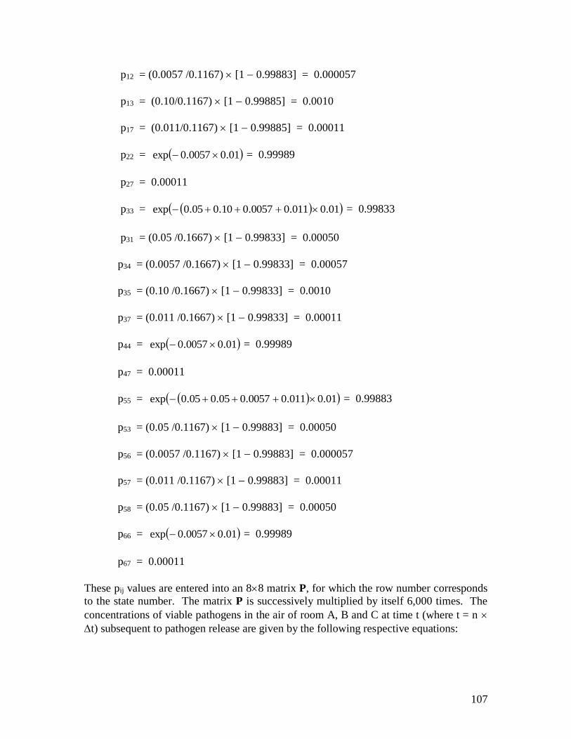
107
p12 = (0.0057 /0.1167) [1 0.99883] = 0.000057
p13 = (0.10/0.1167) [1 0.99885] = 0.0010
p17 = (0.011/0.1167) [1 0.99885] = 0.00011
p22 = 01.00057.0exp = 0.99989
p27 = 0.00011
p33 = 01.0011.00057.010.005.0exp = 0.99833
p31 = (0.05 /0.1667) [1 0.99833] = 0.00050
p34 = (0.0057 /0.1667) [1 0.99833] = 0.00057
p35 = (0.10 /0.1667) [1 0.99833] = 0.0010
p37 = (0.011 /0.1667) [1 0.99833] = 0.00011
p44 = 01.00057.0exp = 0.99989
p47 = 0.00011
p55 = 01.0011.00057.005.005.0exp = 0.99883
p53 = (0.05 /0.1167) [1 0.99883] = 0.00050
p56 = (0.0057 /0.1167) [1 0.99883] = 0.000057
p57 = (0.011 /0.1167) [1 0.99883] = 0.00011
p58 = (0.05 /0.1167) [1 0.99883] = 0.00050
p66 = 01.00057.0exp = 0.99989
p67 = 0.00011
These pij values are entered into an 88 matrix P, for which the row number corresponds
to the state number. The matrix P is successively multiplied by itself 6,000 times. The
concentrations of viable pathogens in the air of room A, B and C at time t (where t = n
t) subsequent to pathogen release are given by the following respective equations:

108
CroomA(t = n t), #/m3 = (n)
11P V
N (8.12)
CroomB(t = n t), #/m3 = (n)
13P V
N (8.13)
CroomC(t = n t), #/m3 = (n)
15P V
N (8.14)
Figure 8.3 answers the first question that was posed, namely, what is the time course of
the airborne viable pathogen concentrations in the three rooms from t = 0 to
t = 60 minutes. The answer to the second question concerning the average density
(# per m2) of viable pathogens on the floor surfaces at t = 60 minutes can be obtained
from the matrix P6000. The relevant quantities are: (6000)
12P = 0.0431, (6000)
14P = 0.0358, and (6000)
16P = 0.0306. Given N = 1.0 106 and a floor area of 33.33 m2 in each room, it
follows that the viable pathogen densities on the floor surfaces are:
Room A: 2
6
m 33.33
101 0.0431 = 1,293 per m2
Room B: 2
6
m 33.33
101 0.0358 = 1,074 per m2
Room C: 2
6
m 33.33
101 0.0306 = 918 per m2
A MATLAB code that implements the numerical solution for this scenario, and generates
Figure 8.3

109
0 10 20 30 40 50 600
1000
2000
3000
4000
5000
6000
7000
8000
9000
10000
Time in minutes
Part
icle
con
cen
trati
on
in
# p
er m
3
RoomA
RoomB
RoomC
Figure 8.3 Particle concentrations in room A, B, and C

110
ADDITIONAL IDEAS ON MODELING PARTICLE FATE AND
TRANSPORT
Emitted particles are rarely uniform in size, but instead comprise a mixture of sizes.
Because the particle settling rate settle depends on particle aerodynamic diameter, each particle size or small range of particles sizes should be considered separately, and the
final answer should be an appropriate combination of the answers for each particle size.
For example, in the previous scenario, what if 1.0 106 pathogens associated with
particles having da = 30 m were released into the air of room A, along with the 1.0 106
pathogens associated with particles having da = 3 m? The overall pathogen
concentration in air and the pathogen density on the floor is the sum of the solutions for
the pathogens associated with each particle size. The concentration in room A air
increases two-fold at the outset, but there are much smaller increases in the pathogen
concentration in the air of rooms B and C. At t = 60 minutes after release, the viable
pathogen concentrations on the floor of rooms A, B and C are, respectively, 29,100 per
m2, 6,010 per m2, and 2,400 per m2, which is a 12-fold range. When we considered only
the 3 m particles, the correspond-ing deposition values were 1,290 per m2, 1,070 per m2 and 920 per m2, which is a 1.4-fold range. The reason for the 23-fold increase on the
floor of room A (29,100 per m2 versus 1,290 per m2) and the greater range of values
across the three rooms (12-fold versus 1.4-fold) is that the 30 m particles rapidly settle,
so only a small portion ever leave room A. This fact also accounts for the minor increase
in the pathogen concentration in the air of rooms B and C despite the release of twice as
many pathogens.
An important transport mechanism within a room is turbulent eddy diffusion. Air is
always in motion, and a good deal of the motion can be viewed as random. One can
envision that a random eddy or swirl of air grabs a small packet of particles and moves
the particles to a nearby location, then another eddy or swirl of air grabs some of the
latter particles and moves them to a different nearby location, and so forth. In
probabilistic terms, turbulent eddy diffusion signifies that the particles take a three-
dimensional random walk in room air. In fact, the equation for diffusion in three
dimensional space is based on this random walk assumption. The random walk can be
understood in discrete time as follows. At the start of a time step, a particle flips three
fair coins. The outcome of the first coin flip (heads or tails) indicates which direction the
particle moves on the x-axis, the outcome of the second coin flip indicates which
direction the particle moves on the y-axis, and the outcome of the third coin flip indicates
which direction the particle moves on the z-axis. This turbulent eddy motion can be
superimposed on an average directional air flow termed bulk advective flow (which is
termed “drift” in random walk theory).
Particle (and molecule) transport by turbulent eddy diffusion can be incorporated into the
Markov chain model as a first-order rate constant, but this requires conceptually
segmenting room air into a reasonably large number of small compartments. In any time
step, three transport mechanisms can act on a particle in an interior room air cell –
turbulent eddy diffusion, bulk advective air flow, and gravitational settling. Due to the
greater number of states in the Markov matrix (on the order of hundreds to thousands),

111
the computer coding is more complicated than the simple MATLAB codes that have been
presented. One of the readings describes a Markov chain fate-and-transport model for
molecular contaminants that incorporates turbulent eddy diffusion. Validation of the
predictive ability of an analogous Markov chain fate-and-transport model for particles is
a current research focus of the author.
Finally, particles can deposit onto the walls and ceilings of a room by mechanisms other
than gravitational settling. For relatively large particles with da > 10 m that are released in the interior core of a room, wall and ceiling deposition tend to be negligible compared
to floor deposition. The reason, in part, is that the large particles settle fairly rapidly and
do not reach the wall and ceiling surfaces. However, if the release point is next to a wall
surface, we would expect a non-negligible amount of deposition onto the wall.
Deposition loss onto walls and ceilings for relatively small particles with da < 10 m does
occur and should properly be considered in fate-and-transport modeling. Unfortunately,
at present there is only a small data base on which to base such modeling.
EXAMPLE 8.4 FATE AND TRANSPORT ON SURFACES
(FOMITES)
It is thought that a substantial portion of human respiratory tract infections are
transmitted via contaminated hand contact with the lips, the conjunctivae of the eyes, and
the nostrils, with subsequent transport to target tissue sites in the oro- and naso-
pharyngeal region. Aside from rhinovirus infection, which has been shown to occur
following contact of the nasal and conjunctival mucosa with fingertips seeded with virus,
the evidence for the hand contact route is indirect albeit substantial. A meta-analysis of
eight selected intervention studies geared toward the general public showed a 24%
decrease in respiratory illness relative to control groups due to hand washing measures.
The dose of pathogens delivered to facial target membranes due to hand touches logically
should depend on: (i) the rate of hand contact (number per unit time) with environmental
surfaces (often termed fomites) and facial target membranes, (ii) the concentration of
pathogens on the touched environmental surfaces (fomites), and (iii) the transfer
efficiencies from surface-to-hand and from hand-to-facial target membrane during the
touch.
In general, there are few published data on the values of these exposure factors. Data on
the rate of hand contact with facial target membranes come from two studies. Hendley,
et al., observed a total of 124 adults seated either in an amphitheater or a Sunday school
for periods of 30 to 50 minutes each, such that there were 89 person-hours of observation.
Hendley reported 29 episodes of nose-picking (0.33 hr1) and 33 episodes of eye-rubbing
(0.37 hr1); the degree and duration of contact that qualified as nose-picking and eye-
rubbing were not defined (“Transmission of rhinovirus by self-inoculation,” New Engl. J.
Med. 288:1361-1364, 1973). In a study by Daniel Best and this author, 10 adults were
observed for 3 hours each (30 person-hours of observation) while the subjects sat alone in
a room performing office-type work. The observed rates of contact with the nostrils, eyes
and lips were, respectively, 5.3 hr 1, 2.5 hr1, and 8.0 hr1. At least 50% of the nostril

112
and eye touches observed could be classified as, respectively, nose-picking and eye-
rubbing, although qualitative judgment is used for that classification. Assuming there
was a true difference in the rates of nose-picking and eye-rubbing observed in the two
studies, one reason might be that the subjects who were alone did not feel as socially
inhibited as they would in a group setting.
A relatively simple, generic Markov chain model is now posed for transfer from room
environmental surfaces to facial target membranes. The scenario is that a person enters a
room with contaminated surfaces and remains in the room for 60 minutes. The aim is to
estimate the number of viable pathogens transferred to facial target membranes during
this 60-minute exposure period. The values of the input factors will depend on the
specific pathogen and scenario considered.
Let state 1 denote room environmental surfaces that can be touched by a person in the
room. For a given pathogen, let Csurface (number of pathogens per cm2) be the average
viable pathogen density on those environmental surfaces at time zero when a person
enters the room. Substantial variability in pathogen density on different room surfaces is
expected. The total surface area available for touching is denoted Atotal (cm2). Pathogens
are lost from surfaces by die off with first-order rate constant dieoffsurface (min1), and by transfer to the hands of the person who touches the surfaces. For simplicity, we consider
that the same finger pad is always used to touch surfaces, and this finger pad has area
Afinger (cm2). We also assume that the room surface area touched by this finger pad per
touch equals the same Afinger value. Thus the fraction of Atotal contacted per touch is
Afinger Atotal. Let state 2 denote the finger pad. The fraction f12 denotes the fraction of
pathogens on the touched surface (with area Afinger) that are transferred to the finger pad
per touch. Thus, the number of pathogens transferred per touch is Csurface Afinger f12. This number is a fraction of the total number of pathogens on the surfaces available for
touching, where the total number is Csurface Atotal. Let Hsurface denote the rate of touching
room environmental surfaces (touches per minute). The first-order rate of pathogen loss
from room environmental surfaces due to touching, denoted touch (min1), is the product of the fraction of all pathogens transferred to the finger pad per touch and the touch rate,
or:
touch12 = total
12finger
A
fA Hsurface
Pathogens are lost from the finger pad by die off with first-order rate constant dieofffhand
(min1), by transfer back to room environmental surfaces upon touching those surfaces, and by transfer to facial target membranes upon touching those membranes. Let f21
denote the fraction of pathogens on the finger pad that are transferred back to the room
environmental surface per touch. The first-order rate of pathogen loss from the finger
pad to room environmental surfaces due to touching, denoted touch21 (min1), is:
touch21 = f21 Hsurface

113
Let state 3 denote facial target membranes (the conjunctivae, the nostrils and the lips).
Let Hface denote the rate that the finger pad touches facial target membranes (touches per
minute), and let f23 denote the fraction of pathogens on the finger pad that are transferred
to one of these membranes per touch. For simplicity, f23 is assumed to be the same value
for all three membranes. The first-order rate of pathogen loss from the finger pad to
facial target membranes due to touching, denoted touch23 (min1), is:
touch23 = f23 Hface
For simplicity, it is assumed that pathogens transferred to facial target membranes cannot
be removed by subsequent touching, and that they remain active until they reach target
tissue sites in the oro- and nasopharyngeal region. Thus, all the pathogens transferred to
state 3 comprise the pathogen dose. Let state 4 be pathogen inactivation. Pathogens that
enter state 4 never leave.
The single-step transition probabilities for state 1 (room environmental surfaces) are:
p11 = texp acedieoffsurftouch12
p12 = acedieoffsurftouch12
touch12
[1 p11]
p14 = acedieoffsurftouch12
acedieoffsurf
[1 p11]
The single-step transition probabilities for state 2 (the finger pad or hand) are:
p22 = texp dieoffhandtouch23touch21
p21 = dieoffhand23touchtouch21
touch21
[1 p22]
p23 = dieoffhand23touchtouch21
touch23
[1 p22]
p24 = dieoffhand23touchtouch21
dieoffhand
[1 p22]
The single-step transition probabilities for state 3 (the facial target membranes) are p33 =1
with the others equal to zero. The single-step transition probabilities for state 4 (patho-
gen inactivation) are p44 =1 with the others equal to zero.

114
At this point, the conceptual work of defining the loss rates and the single-step transition
probabilities is completed. Now we assign numerical values for the factors Atotal, Afinger,
Hsurface, Hface, dieoffsurface, dieoffhand, Csurface, f12, f21, f23 and t. Let Atotal = 10,000 cm2 and
let Afinger = 2 cm2. Let the touch rate to surfaces be Hsurface = 2 min1, and the touch rate
to facial target membranes be Hface = 0.17 min1 (about 10 per hour). Let dieoffsurface =
0.011 min1, which corresponds to a half life on room surfaces of about one hour. Let
dieoffhand = 0.069 min1, which corresponds to a half life on the hands of about 10 minutes.
Let Csurface = 100 per cm2, such that the total number of pathogens in state 1 at time zero
is N = Csurface Atotal = 1.0 106. Let t = 0.01 min. It follows that:
touch12 = [(Afinger f12) Atotal] Hsurface =
[(2 cm2 0.005) (10,000 cm2)] (2 min1) = 2 106 min1
touch21 = f21 Hsurface = 0.005 (2 min1) = 0.010 min1
touch23 = f23 Hface = 0.35 (0.17 min1) = 0.0595 min1
dieoffsurface = 0.011 min1, as given
dieoffhand = 0.069 min1, as given
In turn:p11 = 01.0011.0000002.0exp = 0.99989
p12 = (0.000002 /0.011002) [1 0.99989] = 2 108
p14 = (0.011/0.011002) [1 0.99989] = 0.00011
p22 = 01.0069.00595.0010.0exp = 0.99862
p21 = (0.010/0.1385) [1 0.99862] = 0.0001
p23 = (0.0595/0.1385) [1 0.99862] = 0.000595
p24 = (0.069/0.1385) [1 0.99862] = 0.00069
p33 = 1
p44 = 1
These pij values are entered into a 44 matrix P, for which the row number corresponds
to the state number. The matrix P is successively multiplied by itself 6,000 times. The

115
number of viable pathogens transferred to facial target membranes at t = 60 minutes after
room entry is: N (6000)
13P = (1 106) (3.4 105) = 34 pathogens.
Sample MATLAB code for running the well-mixed room particle release model
% samplecode1.m
% P is the 3x3 Markov matrix
P = zeros(3,3);
P(1,1) = 0.99935;
P(1,2) = 0.00050;
P(1,3) = 0.00015;
P(2,2) = 1;
P(3,3) = 1;
% Check that the row entries in P sum to one
CHECKP = zeros(3,1);
for i = 1:3
CHECKP(i,1) = sum(P(i,1:3));
end
[CHECKP]
N = 1000000; % number of particles released at time zero
V = 100; % room volume in m3
CONCENTRATION = zeros(12001,1); % concentration in # per m3
CONCENTRATION(1,1) = N/V;
CONCENTRATION(2,1) = (N/V)*P(1,1);
TIME = zeros(12001,1); % time in steps of 0.01 minute
TIME(2,1) = 0.01;
PTEMP = P;
for n = 2:12000
TIME(n+1,1) = n/100;
PTEMP = PTEMP*P;
if n == 3
[PTEMP]
end
CONCENTRATION(n+1,1) = (N/V)*PTEMP(1,1);
end
% Check that the row entries in PTEMP sum to one
CHECKPTEMP = zeros(3,1);
for i = 1:3
CHECKPTEMP(i,1) = sum(PTEMP(i,1:3));
end
[CHECKPTEMP]

116
plot(TIME, CONCENTRATION)
xlabel('Time in minutes')
ylabel('Particle concentration in # per m^{3}')

117
Sample MATLAB code for running the three room particle release model
% samplecode2.m
da = 3; % aerodynamic diameter in um
V = 100; % m3
H = 3.0; % m
FA = 33.333; % m2
Q = 5; % m3/min
beta = 5; % m3/min
VTS = 0.0018*(da^2)*(1 + (0.166/da)); % m/min
deltat = 0.01; % 0.01 minute
lambdaAB = (Q+beta)/V;
lambdaBA = beta/V;
lambdaBC = (Q+beta)/V;
lambdaCB = beta/V;
lambdaexhaust = Q/V;
lambdasettle = VTS/H;
lambdadieoff = 0.011; % per minute, half life of about 1 hour
% P is the 8x8 Markov matrix
P = zeros(8,8);
totalrate1 = lambdaAB + lambdasettle + lambdadieoff;
p11 = exp(-totalrate1*deltat)
p12 = (lambdasettle/totalrate1)*(1 - p11)
p13 = (lambdaAB/totalrate1)*(1 - p11)
p17 = (lambdadieoff/totalrate1)*(1 - p11)
totalrate2 = lambdadieoff;
p22 = exp(-totalrate2*deltat)
p27 = 1- p22
totalrate3 = lambdaBA + lambdaBC + lambdasettle + lambdadieoff;
p33 = exp(-totalrate3*deltat)
p31 = (lambdaBA/totalrate3)*(1 - p33)
p34 = (lambdasettle/totalrate3)*(1 - p33)
p35 = (lambdaBC/totalrate3)*(1 - p33)
p37 = (lambdadieoff/totalrate3)*(1 - p33)
totalrate4 = lambdadieoff;
p44 = exp(-totalrate4*deltat)
p47 = 1- p44
totalrate5 = lambdaCB + lambdaexhaust + lambdasettle + lambdadieoff;
p55 = exp(-totalrate5*deltat)

118
p53 = (lambdaCB/totalrate5)*(1 - p55)
p56 = (lambdasettle/totalrate5)*(1 - p55)
p57 = (lambdadieoff/totalrate5)*(1 - p55)
p58 = (lambdaexhaust/totalrate5)*(1 - p55)
totalrate6 = lambdadieoff;
p66 = exp(-totalrate6*deltat)
p67 = 1- p66
P(1,1) = p11; P(1,2) = p12; P(1,3) = p13; P(1,7) = p17;
P(2,2) = p22; P(2,7) = p27;
P(3,1) = p31; P(3,3) = p33; P(3,4) = p34; P(3,5) = p35; P(3,7) = p37;
P(4,4) = p44; P(4,7) = p47;
P(5,3) = p53; P(5,5) = p55; P(5,6) = p56; P(5,7) = p57; P(5,8) = p58;
P(6,6) = p66; P(6,7) = p67;
P(7,7) = 1;
P(8,8) = 1;
% Check that the row entries in P sum to one
CHECKP = zeros(8,1);
for i = 1:8
CHECKP(i,1) = sum(P(i,:));
end
[CHECKP]
N = 1000000; % number of particles released at time zero
CONCENTRATION = zeros(6001,3); % concentration in # per m3
CONCENTRATION(1,1) = N/V; % concentration in room A air at t = 0
CONCENTRATION(2,1) = (N/V)*P(1,1); % concentration in room A air at t = 0.01
CONCENTRATION(2,2) = (N/V)*P(1,3); % concentration in room B air at t = 0.01
TIME = zeros(6001,1); % time in steps of 0.01 minute
TIME(2,1) = 0.01;
PTEMP = P;
for n = 2:6000
TIME(n+1,1) = n/100;
PTEMP = PTEMP*P;
CONCENTRATION(n+1,1) = (N/V)*PTEMP(1,1); % concentration in room A air
CONCENTRATION(n+1,2) = (N/V)*PTEMP(1,3); % concentration in room B air
CONCENTRATION(n+1,3) = (N/V)*PTEMP(1,5); % concentration in room C air
end
X = PTEMP(1,:)'

119
% Check that the row entries in PTEMP sum to one
CHECKPTEMP = zeros(8,1);
for i = 1:8
CHECKPTEMP(i,1) = sum(PTEMP(i,:));
end
[CHECKPTEMP]
plot(TIME,CONCENTRATION(:,1),'-',TIME,CONCENTRATION(:,2),'--
',TIME,CONCENTRATION(:,3),'.-')
xlabel('\bf\fontname{times}\fontsize{12}Time in minutes')
ylabel('\bf\fontname{times}\fontsize{12}Particle concentration in # per m^{3}')
%gtext('\bf\fontname{times}\fontsize{12}\leftarrowRoomA')
%gtext('\bf\fontname{times}\fontsize{12}\leftarrowRoomB')
%gtext('\bf\fontname{times}\fontsize{12}\leftarrowRoomC')

120
Sample MATLAB code for running the surface-to-hand-to-face transfer model
% samplecode3.m
AreaTotal = 10000; % cm2
AreaFinger = 2; % cm2
f12 = 0.005; % 0.05% per touch
f21 = 0.005;
f23 = 0.35;
Hsurface = 2; % 2 per minute
Hface = 0.17; % 0.17 per minute = 10 touches per hour
deltaT = 0.01;
lambdadieoffsurface = 0.011; % per minute, half-life of 60 minutes
lambdadieoffhand = 0.069; % per minute, half-life of 10 minutes
lambdatouch12 = (AreaFinger/AreaTotal)*f12*Hsurface;
lambdatouch21 = f21*Hsurface;
lambdatouch23 = f23*Hface;
totalrate1 = lambdatouch12 + lambdadieoffsurface;
p11 = exp(-totalrate1*deltaT);
p12 = (lambdatouch12/totalrate1)*(1 - p11);
p14 = (lambdadieoffsurface/totalrate1)*(1 - p11);
totalrate2 = lambdatouch21 + lambdatouch23 + lambdadieoffhand;
p22 = exp(-totalrate2*deltaT);
p21 = (lambdatouch21/totalrate2)*(1 - p22);
p23 = (lambdatouch23/totalrate2)*(1 - p22);
p24 = (lambdadieoffhand/totalrate2)*(1 - p22);
p33 = 1;
p44 = 1;
% P is the 4x4 Markov matrix
P = zeros(4,4);
P(1,1) = p11;
P(1,2) = p12;
P(1,4) = p14;
P(2,1) = p21;
P(2,2) = p22;
P(2,3) = p23;
P(2,4) = p24;
P(3,3) = p33;
P(4,4) = p44;

121
% Check that the row entries in P sum to one
CHECKP = zeros(4,1);
for i = 1:4
CHECKP(i,1) = sum(P(i,1:4));
end
[CHECKP]
N = 1000000; % number of pathogens on 10,000 cm2 of surface
PTEMP = P;
for n = 1:6000
PTEMP = PTEMP*P;
end
% Check that the row entries in PTEMP sum to one
CHECKPTEMP = zeros(4,1);
for i = 1:4
CHECKPTEMP(i,1) = sum(PTEMP(i,1:4));
end
[CHECKPTEMP]
DOSE = N*PTEMP(1,3);
[PTEMP(1,:)]

122
Chapter 9: Introduction to Deterministic Dynamic Disease Modeling
Jim Koopman
Analyzing dynamics rather than risks
Controlling infectious disease often requires a different mental set and a different set of
analytic skills than the risk factor identification and elimination mentality that dominates
classical epidemiology teaching. Instead of seeking to understand why some individuals
in a population develop disease while others don’t, infection control often requires us to
seek explanations for why infection flows and grows within a population. Instead of
using risk or rate ratio measures, odds ratio measures, risk and rate differences, and other
simple relationships between presumably independent individuals with and without a risk
factor to seek explanations for disease patterns in populations, infection control requires
the estimation of parameters that reflect interactions between individuals such as contact
rates, transmission probabilities, network cluster sizes and diameters, network
connectedness measures and other measures. For infection control we must think about
where and how infection is flowing through a population and what we can do about it.
That requires a whole different way of thinking. The objective of the exercise we will do
in this QMRA session is to get you into this other mode of thinking so that when you
have public health responsibilities you will be better prepared to think about the right
issues and frame the questions you should be asking in a more effective way.
Most analyses in epidemiology assess risk factor effects under the assumption that the
outcome of “exposure” to a risk factor in one individual cannot change the outcome of
“exposure” in another person. (Note we often call individuals with a risk factor an
"exposed" group but here we will try to reserve the term “exposed” for individuals who
have come in contact with infectious individuals.) What that means is that if the risk
factor is not washing your hands after going to the bathroom, that if you get infected as
the result of such a risk factor you do not change the risks experienced by other
individuals. Most statistical analyses of risk factor effects make this independence
between individuals assumption. (Note that independence between variables in a single
individual is a wholly different independence issue.)
An important issue in infectious disease epidemiology is how the pattern of connections
from one individual to another causes infection to flow through a population, epidemics
to grow, or endemic levels of infection to be sustained. That is to say, an important issue
in infectious disease epidemiology is population dynamics and how dependencies
between outcomes in different individuals determine those population dynamics. So
instead of using models that assume no infection transmission like the data models that
you have learned in statistics courses, we need to use models that parameterize (capture
and express) the true nature of this dependency that we need to understand in order to
control infection. Instead of thinking about individual risks, we need to think about
population dynamics. We need to get our heads turned around from classical
epidemiological thinking if we are going to effectively control infections.

123
Infection transmission models and models of infection and immunity processes within
individuals are becoming especially important in using powerful new sources of
molecular information about infection that is becoming available. Using micro-array
chips, laboratories on a chip, and other magnificent technologies, it is increasingly cost-
effective to gather information on the genetic sequences of infectious agents, the genetic
make up of hosts that influence their response to infection, and on myriad aspects of the
host response to infection. The efficient use of this information requires analyses that
make correct assumptions about dependencies between individuals or dependencies
between infectious agents, host genetics, and host immune responses. Understanding the
basics of infection transmission models is needed to use genetic data to help analyze
infection flow. In this regard, infection transmission model analyses are becoming an
important part of bioinformatics.
TYPES OF MODELS
Infection transmission system models express the non-linear dynamics of infection spread
through populations. To ensure you understand what is meant by non-linear dynamics of
infection transmission recommended reading includes “The Ecological Effects of
Individual Exposures and Nonlinear Disease Dynamics in Populations” (Koopman &
Longini, 1994). Another background article that is more comprehensive but more
advanced covering infection transmission system modeling is “Modeling Infection
Transmission” (Koopman, 2004).
There are many different forms of infection transmission models that can be used for
different purposes. We will discuss a particular modeling form that makes a peculiar set
of assumptions that greatly facilitate computer analyses and that do not require you to
have great programming or mathematical skills. These are called deterministic
compartmental models. In our case, the compartments contain different segments of
population defined by their characteristics such as their infection and immunity state or
their risk factor status. Risk factors might affect their susceptibility, their contagiousness
if infected, or behaviors that affect their exposure to someone who could transmit
infection to them.
The particular form of model we will use is called a deterministic compartmental (DC)
model. Deterministic means that chance is not playing a role. Every time you run the
computer models you construct you will get exactly the same results as long as the
starting conditions and parameters are the same. There is no "Monte Carlo" aspect to the
model implementation where an individual's chance of experiencing something is
determined by a role of the dice. In fact, there are no individuals in the model for chance
to act on.
Well, you may ask, if there are no individuals in the model, what are we modeling and
how do we deal with interactions between individuals that might occur with specified
probabilities and that transmit infection if the interaction takes place with certain
probabilities? The answer is: We are modeling continuous segments of population. We
assume that any segment of population, no matter how small, can be further subdivided.

124
That is in part what we mean by continuous. We assume that any tiny segment of the
population can be further subdivided and also we assume that the population is made up
of discrete individuals. Those two assumptions together imply that we are assuming that
the population we are modeling is of infinite size. In practice very large does not differ
from infinite. But when we have compartments that we want to correspond to just a
handful of individuals, the difference in our assumed infinite size and our desired handful
size may be important.
Whenever numbers are small, chance might be influencing what fraction of individuals
experience an outcome. But as population size becomes infinite, the variation in the
fraction of the total population that experiences an outcome becomes infinitesimally
small. Thus our properties of infinite population size and deterministic behavior go
together. The deterministic models just examine the mean behavior of infinite size
populations. Sometimes we may be really interested in the chance of events in small
populations. Say for example we are interested in predicting when polio will be
eradicated. Well, when we get close to eradication, there are by definition very few
individuals in the infected compartments. When the last transmission from any case
occurs will be a chance event. In our deterministic continuous population compartmental
models eradication will never occur. Some fraction of the population will always be
being cured but that means some fraction will always be being left infected. That fraction
may be infinitesimally small. It may be too small to register so it shows up on the
computer as zero. But that is not theoretically zero. Only stochastic models can get us to
theoretical zero infections.
You will note that even though we formally assume that the population we are modeling
is continuous, we speak of interactions between different segments of our population or
rates of change in different segments of our population as if they were interactions
between individuals and risks of events occurring to individuals.
For this QMRA session we do not have to learn a whole lot of words that further classify
the types of models we analyze within the set of deterministic models of continuous
populations. But if you want to impress someone (other than a mathematician) with what
you are learning you can say that you have learned to construct and numerically analyze
first order, Markovian, scalar, autonomous, homogeneous, non-linear systems of ordinary
differential equations.
First order just means that we model rates of change, not rates of change of the rates of
change, which would be second order. Markovian is something you might want to learn.
It means that what is happening in a model at any point in time is just a function of the
model states at that point in time. Another word for Markovian is "memoryless". What
happens in the model does not depend upon what was going on in the model at some past
point in time. It only depends on the current state. The model does not have to
remember anything from its past to calculate what happens next. It is this Markovian
property, together with the deterministic property, that makes DC models so easy to
analyze on the computer. The computer does not have to keep in its memory what the
state of the model was in the past and use those past states to help determine what

125
happens next. That greatly cuts down on both memory and calculations. But the real
world is not usually “memoryless”. This Markovian characteristic, like the continuous
population characteristic, is an unrealistic simplifying assumption we make in order to
have a tractable model.
To address many important problems we need models with discrete individuals. Such
models are harder to program and to analyze because chance events may lead to different
outcomes. Thus a single outcome is not enough as is the case with deterministic
compartmental models. The ideal in analyzing a discrete individual stochastic model is
to keep track of the expected distributions of numbers of individuals in any state. That is
a really big and hard task so for such models we often just do a series of Monte Carlo
simulations that give us one particular realization of a chance process. If we do hundreds
of such simulations, that gives us a feel for the shapes of distributions of expected sizes
of compartments. But that is a lot of work and it takes a lot of programming skill.
Therefore we will not be dealing with this sort of model in this course. Epidemiology
students who want to learn this sort of modeling take courses in the Center for the Study
of Complex Systems. If you want to go on to a higher degree in infectious disease
epidemiology, we strongly recommend these courses.
There are many other model types besides continuous population deterministic
compartmental models and discrete individual stochastic models. But for now we don't
need to worry about these. It is better that we get on with our task.
Goals of infection transmission modeling
There are many different ways to classify the purposes of modeling. I variously use
classifications that have from 5 to 28 different categories. Here is the five category
division of purposes.
1. Generate and clarify insights into non-linear processes
All processes in the world have non-linear dynamics at some level. One reason
epidemiologists don’t include more non-linear dynamics in their models is that non-linear
dynamics often don’t fit in well with the intuitive predictive processes that have evolved
in human cognitive processes. Ontologically, it is not until the adolescent years that
many intuitive predictions of joint effects of two forces come into play. When two
different non-linear processes interact in a model, intuitive prediction of effects usually
breaks down. But experience analyzing simple systems can help build the intuitive
capacities needed to be a great scientist. Simple non-linear systems can generate
incredibly complex patterns. Computer simulation experience with such systems can be
an essential learning experience for pursuing any of the subsequent four purposes listed
here. It is almost wholly for the purpose of providing you with insights about the non-
linear dynamics of infection transmission in populations that we pursue modeling
analyses in this course. You will be learning to use a software tool that will be helpful to
you in advancing and clarifying your thinking about infection transmission or about many
other types of systems. This tool will help you to learn on your own.
2. A base for formal theory presentation and analysis

126
When a mathematical or computer simulation relationship is found to express a real
world relationship of interest, the potential for scientific progress is expanded.
Mathematics and computer science have developed powerfully productive traditions for
advancing the analysis of systems and whenever these can be applied to any system,
more compact and comprehensible ways of communicating and analyzing theory become
available. Epidemiology does not have the tradition of having separate theorists who
purely dedicate themselves to advancing theory as other sciences like physics, chemistry,
computer science, and some others do. That is because the theories epidemiology has
been developing are simple exposure causes disease types of theory expressed in terms of
risks rather than dynamic processes. As epidemiologists begin formulating more
universal theories that encompass broader sets of conditions, epidemiology theories will
inevitably involve non-linear dynamics and will undoubtedly be more complex and
provide a better basis for new theory construction. Then the need for more
epidemiologists to dedicate themselves more strongly to theory elaboration and
development will be more evident.
3. Prediction
The main virtue of sound theory is predictive power. The predictive power of regression
relationships is always limited. If one had lots of data on the rate of speed at which
objects fall under different conditions on earth, one could make just as good predictions
about rates of fall using regression relationships as one could make using gravity and
friction theories. But one could not make any predictions for the moon or other planetary
bodies as one could by using the theoretical relationships. Epidemiology is in a far less
favorable position for regression relationships to predict disease risks than physics is to
use regression relationships to predict falling body rates. The reason is the evolved
complexity of processes affecting disease risks. Yet epidemiology continues to make
most predictions on the basis of data relationships with little theory.
All perception requires both data and theory. All prediction requires both data and theory.
And the role of theory in either perception or prediction cannot be separated from the role
of data. Data alone or theory alone can do nothing. They must work together.
Epidemiology makes predictions on the basis of observed risks in the past. But
conditions change from the past to the future. Epidemiology makes predictions of risks
in one population from observations on another. Yet if conditions differ, only
relationships based on solidly verified theory will continue to hold across populations or
across time. As we enter an era where the complexities and variations in each individual
become a basis for assessing their risks, the need for predictive theory becomes greater.
Theoreticians are needed to develop predictions of risks under different conditions. Good
theory evaluation will allow one to specify the conditions under which competing
theories make different predictions for things that have up to now not been observed.
Observations then become the basis for distinguishing theories. No observations,
however, can be theory free. As much as possible it is useful to be able to specify the
theoretical assumptions that lie behind any observation. That helps prediction advance
science and it helps public health make inferences about what actions should be taken.
We will make brief comments later on how that works after discussing different types of
models.

127
4. Study design
Studies need to be designed so that they lead to valid inferences with minimal
expenditure of resources. Epidemiologists tend to categorize study designs into a limited
number of classes and then make rules for what classes are to be used under what
conditions. But this limits the creativity that should go into study design and the number
of options that should be explored. Study design is ideally carried out by specifying a
series of causal models that one thinks might apply to the situation where one is seeking
to make a particular inference and then imposing different study designs that will
generate the data from those underlying causal models. Then one assesses the power and
validity of inferences from those study designs under different causal model
specifications. Modern computer simulation methodology and analytic power makes this
a much more feasible process now than it was at the turn of the century. But study design
really requires stochastic discrete individual models.
5. Data analysis
If the model that one is using to analyze data does not correspond to the causal processes
that generated the data and upon which the inferences being sought depend, then one
should always feel that inferences based on that data analysis might not be robust.
Fortunately there have been many advances in statistics, both in biostatistics and in other
sciences, like physics, that now make it much easier to build statistical analyses on the
basis of causal models. These are usually highly computer intensive. The biggest driver
of new advances in this regard is not necessarily greater micro-processor power and
greater numbers of micro-processors used. As much a driver of progress in this area is
the development of ingenious new algorithms that computer scientists and other scientists
come up with.
Again using transmission system models for data analysis is beyond this course. We will,
however, learn a little bit about fitting models to data. That is a sort of data analysis and
the methods we will learn are parameter estimation methods. They are just not the best
parameter estimation methods. The best methods are based on discrete individual models
which we do not use in this course.

128
Chapter 10: Environmental Infection Transmission System Models
Joseph Eisenberg
GOAL
The overall objective of this unit is to learn about environmental infection transmission
system models and their importance in quantitative microbial risk assessments. This
chapter contains two manuscripts, a short introduction to the software package MATLAB,
and a lab worksheet. The two manuscripts: 1) 'Dynamics and control of infections
transmitted from person to person through the environment'; and 2) 'Disease transmission
models for public health decision making: analysis of epidemic and endemic conditions
caused by waterborne pathogens' will provide background reading for your lecture. The
lab worksheet will be completed during the computer lab following the lecture. The lab
activities will use MATLAB.
OVERVIEW OF MATLAB
MATLAB is a high performance language for technical computing. It integrates
computation, visualization, and programming in an easy-to-use environment. MATLAB
is an interactive system whose basic data element is an array.
The command window is the primary window in which you communicate with the
MATLAB interpreter. The MATLAB displays a prompt (>>) indicating that is ready to
accept commands from you.
NOTE: MATLAB is ‘case-sensitive.’ This means that MATLAB distinguishes between
upper and lower case letters in names of variables and scripts. Incorrectly using
capitalized or non-capitalized letters may lead to undesirable results.
BRIEF BACKGROUND ON SOME USEFUL MATLAB FUNCTIONS
MATLAB Variables
MATLAB permits the assignment of variables in the workspace.
>> x=5
>> y=5
MATLAB has now stored the variables x and y as 5. Mathematical operations can then
be performed on assigned MATLAB variables.
>> x*y
Results from mathematical operations will be displayed in the workspace.
To look at the assigned variables in the MATLAB workspace use the whos command.

129
>> whos
To clear all the assigned variable from the workspace, use the clear command. Specific
variables can be cleared by including their name following the clear command.
>> clear
>> clear x
MATLAB SCRIPTS (M-FILES)
When creating and running simulations, we may want to rerun the simulation under
different conditions, e.g. after making small adjustments to parameters in the model.
Repeating these steps each time can be tedious, therefore MATLAB allows you to write
scripts, which are lines of instructions that you can save in a file. To create a script you
would open up a new M-file using the MATLAB editor (in the MATLAB command
window select file, new, m-file). Scripts can then be saved on your computer.
Scripts are executed by entering their name into the workspace (ex. runEITS1.m).
>> run EITS1
Accessing MATLAB Scripts (M-files)
To access old scripts or previously written scripts, you must assign the “Current
Directory” of MATLAB to the folder where the scripts are located.
This can be done by clicking the three dot icon to the right of current directory setting.
A “Browse For Folder” window will pop-up. Select the folder with the desired scripts
and click OK. The left-hand panel should now display all the m-files in this folder (as
well as other MATLAB compatible files). You can view the contents of these files by
double-clicking on them.
History
To save on typing you can recall previous commands by using the key. By
continuously typing the key you can scroll through previous commands. By typing the
first letter of the command you want to recall followed by the key only the commands
starting with that letter will appear.
The diary command creates a copy of all subsequent terminal input and most of the
resulting output to be written on the named file. DIARY OFF suspends it. DIARY ON turns it back on. DIARY, by itself, toggles the diary state. By typing diary followed by
the name of an already existing file, input will be appended to that file.

130
>> diary EITSmodel.txt
>> diary on
>> diary off
Using this diary command you are able to document your work.
Plot
The plot command allows us to create figures from data. The following example creates
a line plot from the data X and Y where X is on the x-axis and Y is on the y-axis.
>> plot(X,Y)
>> grid
The plot command will create a new window that contains the figure. MATLAB allows
us to label the axes.
>> xlabel('Time (days)')
>> ylabel('Infected')
MATLAB can use symbols in plots as well. Here is an example using *'s to mark the
points. MATLAB offers a variety of other symbols and line types.
>> plot(X,Y,'*')
You can also zoom in and out by using the axis command. The syntax is :
axis([Xmin, Xmax, Ymin, Ymax])
>> axis([0 3 90 100])
For a listing of different symbols and line types
>> help plot
TRANSMISSION MODELING IN MATLAB
Introduction to Simulink
Simulink is a software package for modeling, simulating, and analyzing dynamical systems. It
provides a graphical interface for building models as block diagrams, using click-and-drag
mouse operations. With this interface, you can draw the models just as you would with pencil
and paper.
Simulink models are saved as .mdl files. MATLAB will recognize simulink model files in the
current directory. They can be viewed by double-clicking them.
Running Simulink Models
To run a Simulink model, the sim command should be used.
>> sim(‘EITS’,[0,150])
To use the sim command, the model and the duration of the simulation (in this case 0 to
150) must be specified. Depending on the model settings, certain variables will be
assigned values resulting from the simulation.

131
From the QMRA workshop exercise, the EITS Simulink model assigns values to the
variables tout, S, I, and R. The variable tout is the independent time variable (in days)
over which the simulation is run. Its range was specified in the sim command as from 0
to 150. The other variables correspond to vectors where S is the susceptible population, I
is the infected population, and R is the resistant population. These are assigned values
based on the result of the simulation. The results are best viewed by plotting tout against
any of the other variables as is done in the provided scripts.
EXPLORING INTERVENTION OPTIONS USING AN
ENVIRONMENTAL INFECTION TRANSMISSION SYSTEM (EITS)
MODEL
Human infections that pass from one person to another commonly do so through environmental
media, such as air, fomites, food, hands, and water. A transmission model can help understand
the comparative efficacy of one intervention over another. In this exercise we will explore the
properties of a transmission model by examining the following model described in the AJE
manuscript assigned to you.
To simulate this model we will use Matlab, a simulation software package. The model has
already been coded for you. It is called EITS.mdl. Open it up and see what it contains.
We will first explore the basic properties of the model by simulating an outbreak. We will then
explore how the shape of the outbreak curve changes when parameter values are varied. We
will then explore the impact of a decontamination intervention. In our outbreak scenario, there
is a total population of 1000 people. At the start of each simulation, 999 people are free of
infection (susceptible) and 1 person is infected.
Summary of scripts and models used in this lab:
EITS.mdl: Coded that implements the above model
EITS1.m: The script that will simulate EITS.mdl and generate output for Task 1
EITS2.m: The script that will …
EITS3.m: The script that will …
ERISIdt
dE
Idt
dR
IESdt
dI
ESdt
dS
)))((

132
CalcRo.m: The script that calculates the reproductive number (Ro)
Air.m: The script that parameterizes the EITS model for the air transmission mode
Freq.m: The script that parameterizes the EITS model for the frequently touched fomite
transmission mode
Infreq.m: The script that parameterizes the EITS model for the infrequently touched fomite
transmission mode
Exploring model properties
Table 1 provides the estimates from the manuscript and is a key for relating the Matlab
variables to the parameters from the paper.
Table 1
Parameters
Description
Parameter Estimates
3 distinct transmission modes Matlab
label
Air
Frequently
Touched
Fomite
Infrequently
Touched
Fomite
Recovery rate
(1/day)
(gamma) 0.2 0.2 0.2 g
Infectivity
(pi) 0.0517 0.0000693 0.0000693 p
Elimination
rate (1/day) (mu) 8.64 2.88 2.88 m
Deposit rate
(pathogens /
infected /
day)
(alpha) 693 5,244 1040,177 a
Pathogen
Pickup (1 /
person / day) (ro) 0.0000877 0.297 0.0000145 r
Task 1: Simulate an outbreak using parameter values from Table 1
Directions:
1.) Assign parameter values shown in Table 1 to the model. The files containing the
three different parameter sets have been prepared for you. The parameters settings for
airborne transmission are contained in the script air.m, for frequently touched fomite
transmission in the file freq.m, and for infrequently touched fomite transmission in the
file infreq.m. Open up each file to verify that they contain the appropriate values for
Table 1.
2.) To run the model, another script was prepared for you called runEITS1.m. Open up
this file to see what it contains.
3.) To simulate an outbreak, pick one of the parameter file, type in the name (e.g. ‘air’)
and hit enter. Then type in ‘runEITS1’ and hit enter.

133
4.) Two figures should appear in new windows. The first shows the prevalence over time.
The second shows cumulative incidence over time.
5.) Back in the workspace, the values for peak prevalence, time to peak prevalence,
duration of outbreak, and cumulative incidence (total infected) based on the current
parameter set have appeared. These variables were created when running the script.
6.) You can calculate R0 by typing ‘calcR0’ and hitting enter.
7.) Fill out the table below and repeat for the other transmission types.
Transmission
Type
Peak
Cases
(people)
Time of
Peak
(day)
Duration of
Outbreak
(days)
Cumulative
Incidence
(Total Infected)
R0
Air
Frequently
Touched Fomite
Infrequently
Touched Fomite
Task 2: Examine how different parameters affect the epidemic curve
We will now explore the properties of the model by focusing only on air transmission.
Specifically, we will vary each parameter one by one while leaving the others constant in
the airborne settings. Use Table 1 as a reminder of the names of the parameters used in
Matlab. For this task we will simulate outbreaks using the runEITS2.m script.
Example (Changing values): 1.) Set all the parameters to the airborne transmission setting (type in ‘air’ and hit enter).
2.) From Table 1, we see that (g) is set at 0.2/day. To double the recovery rate, type
“g=0.4” into the matlab workspace and hit enter. Now is set at 0.4/day. You can verify this by typing “g” into the workspace and hitting enter.
When doubling the recovery rate, how does this affect the duration of infection?
3.) Now run the outbreak simulation (runEITS2). Note the changes. Is there still an
outbreak? Recalculate R0 (calcR0).
4.) Now try halving gamma, “g=0.1”.
How does the duration of infection change when we halve the recovery rate?
5.) Now conduct the same exploration with each of the other parameters. Only work on
one parameter at a time. After you are finished with your exploration, just type in “air”
again to reset the model back to its original airborne settings. Use the table below as a
guideline for your exploration.
When you change the parameter settings, keep the following questions in mind:

134
What is the interpretation of this parameter?
Which parameter will delay the outbreak?
Which parameter will attenuate the outbreak?
Which parameter will extend the duration of the outbreak?
Predict what will happen to the dynamics before running the simulation.
Feel free to explore under the other transmission settings.
Parameter Potential
Values Outbreak?
Peak
Cases
Time of
Peak
Duration
of
Outbreak
Cumulative
Incidence
(Total
Infected)
R0
g
0.01
0.02 Yes
0.04 No
p
0.04
0.05
0.07
m
7
9
10
a
625
700
800
r
0.00008
0.00009
0.0001
These values were chosen with airborne transmission in mind
Task 3: Determining the role of decontamination in either attenuating or
preventing an epidemic. We will now simulate an intervention in which we increase
rate of environmental elimination.
Which parameter must we change to implement a decontamination intervention? ______
For these simulations we will be using the ‘runEITS3’ script. This script only produces the
cumulative incidence vs. time figure. It also only calculates the total infected. Open it up to
see what it contains.
Airborne Transmission (type in ‘air’ and hit enter):
1.) What is the value of the environmental elimination rate in this transmission system? _____
2.) Simulate the outbreak by typing ‘runEITS3’ and hitting enter.
How many people were infected? _____

135
3.) Now implement an intervention by increasing the decontamination rate parameter by 25%
and rerun the ‘runEITS3’ script.
4.) How many people were infected? _____
(Note that the figure did not reset but now contains both outbreak results. The intervention
result is red.)
5.) How has this intervention affected the incidence?
Now CLOSE THE FIGURE before continuing.
Infrequently Touched Fomite Transmission (type in ‘infreq’ and hit enter):
1.) What is the value of the environmental elimination rate in this transmission system? _____
2.) Simulate the outbreak by typing ‘runEITS3’ and hitting enter.
How many people were infected? _____
3.) Now implement an intervention by increasing the decontamination rate parameter by 25%
and rerun the ‘runEITS3’ script.
4.) How many people were infected? _____
(Note that the figure did not reset but now contains both outbreak results. The intervention
result is red.)
5.) How has this intervention affected the incidence?
Now CLOSE THE FIGURE before continuing.
Frequently Touched Fomite Transmission (type in ‘freq’ and hit enter):
1.) What is the value of the environmental elimination rate in this transmission system? _____
2.) Simulate the outbreak by typing ‘runEITS3’ and hitting enter.
How many people were infected? _____
3.) Now implement an intervention by increasing the decontamination rate parameter by 25%
and rerun the ‘runEITS3’ script.
4.) How many people were infected? _____
(Note that the figure did not reset but now contains both outbreak results. The intervention
result is red.)
5.) How has this intervention affected the incidence?
Which interventions worked?
Which did not?
Why might this be (hint: look at the other parameter settings and R0)?
References:
Eisenberg J.N.S., Brookhart M.A., Rice G., Brown M., Colford J.M. (2002) Disease
transmission models for public health decision making: analysis of epidemic and
endemic conditions caused by waterborne pathogens. Environmental Health Perspectives
110(8)783-790. [Online 17 June 2002]
http://ehpnet1.niehs.nih.gov/docs/2002/110p783-790eisenberg/abstract.html
Sheng L., Eisenberg J.N.S., Spiknall I., Koopman J.S. (2009) Dynamics and Control of
Infections Transmitted from Person to Person through the Environment. American
Journal of Epidemiology. 170(2): 257-265.

136
Chapter 11: Risk Perception, Risk Communication, and Risk
Management
Patrick L. Gurian
GOAL
This chapter considers the social science of risk, that is, how society responds to risk.
This societal response is typically viewed from three perspectives. One is the descriptive
perspective which addresses the question “How do people perceive and react to risk?” A
second viewpoint is prescriptive, concerned with the question of “How should we
communicate with members of society about risk?” A third viewpoint is normative and
asks “How should we manage this risk?” Each of these perspectives is addressed briefly
below.
RISK PERCEPTION
It became apparent fairly soon after a quantitative science of risk assessment was
developed that experts and the public perceive risks in different ways. Cognitive
psychologists investigating these discrepancies developed a body of knowledge related to
how both experts and the public perceive risk (Slovic 1987, Slovic et al. 1980, Slovic et
al. 2004). It was found that expert assessments of risk were driven largely by the
expected number of fatalities. On the other hand, the public’s perception of risk was
actually richer in that it was based on a far broader range of factors. For example, public
perception of risk is driven by not only expected fatalities but also factors such as the
newness of the technology, the threat that the technology might present to future
generations, the dread that the technology inspires on a gut level, the uncertainty
associated with the risk, whether exposure to the risk is voluntary or involuntary, and
many other attributes. In fact, responses to a very wide range of questions can be
correlated to the public’s perception of risk. However, many of these questions would
touch on the same underlying factor. For example, the gut level dread inspired by a risk
and its catastrophic potential would likely be highly correlated, since both stem from the
possibility that a technology might have the potential to produce massive numbers of
casualties in the event of a malfunction. A statistical technique called factor analysis can
be used to interpret highly correlated responses on surveys in terms of a much smaller
number of underlying factors.
In the case of risk perception, three underlying factors have commonly been identified.
The first is usually labeled “dread” and encompasses factors such as the gut-level,
emotional reaction inspired by the risk, the threat the risk presents to future generations,
and the catastrophic potential of the risk (i.e., potential to produce mass casualties). The
second factor is “familiarity”. This includes whether the risk is old or new, whether the
risk is well understood by science or poorly understood by science, and whether it is
something the public deals with on a daily basis or that is less commonly encountered by
the public. The third common factor is the number of people exposed to the risk. Scores
on each of these factors can be computed, and the location of a particular risk in this

137
factor space identified. Figure 11.1 is an example of such a plot with the x-axis showing
the factors score on the dread factor, and the y-axis showing the factor score on the
familiarity factor.
Figure 11.1 Location of risks in factor space (based on Slovic et al. 1980).
Nuclear power is notable as it occupies the space at the extreme upper right hand
quadrant of the factor space. As nuclear power is considered both unfamiliar and dread, it
is a high-profile risk that elicits concern on the part of the public. In general risks in the
upper right hand corner of Figure 11.1 are higher profile risks, which will attract more
public attention. Conversely risks in the lower left hand quadrant scored low on both of
these two factors and will tend to attract less public attention and concern. While this
conceptual framework is very helpful in describing how the public response to various
risks, its ability as a predictive framework to anticipate how the public will react to any
particular risk has not been established.
It is also worth noting how this body of literature is often summarized in an overly
simplistic fashion. In some cases public perception of risk may be described as being
driven solely by “dread”. In other cases, the distinction between voluntary and
involuntary risks may be presented as the only distinction that the public makes. It is true
that emotional factors, such as “dread” impact public perception of risk, and it is also true
that the public tolerates higher levels of risk for voluntary activities such as paragliding,
than for involuntary activities, such as living in an area where a nuclear power plant is
proposed to be located. Nevertheless, one should be mindful that public perception is
Slovic et al.
Nuclear Power
-1
-0.8
-0.6
-0.4
-0.2
0
0.2
0.4
0.6
0.8
1
-1 -0.8 -0.6 -0.4 -0.2 0 0.2 0.4 0.6 0.8 1
Dread: Uncontrollable, Global, Inequitable, Risk to Future Generations,
Affects Me, Increasing
Un
fam
ilia
rit
y:
Un
ob
serv
ab
le,
Dela
yed
Eff
ect,
Un
kn
ow
n t
o S
cie
nce,
New
Bicycles
Automobiles
DynamiteCrime
Hair DyeHigh Profile Risks
Low Profile Risks
Pesticides
Fluoridation

138
driven not just by these two factors of dread and voluntariness, but by a very wide variety
of other factors as well.
A second framework for understanding the public perception of risk is based on
understanding the distinction between analytical and affective thought. Analytical
thought is what the experts do in the formal process of risk assessment. It consists of
applying systematic methods and mathematical models to developing quantitative
estimates of risk. In contrast, affective thought is an emotional, gut-level response. While
the analytical approaches to risk assessment are considered more precise and accurate
than affective approaches, affective methods can actually be seen as necessary shortcuts
for coping with the large number of risks we face given limited cognitive resources.
Affective responses can be seen as a sort of heuristic approach to risk assessment.
As an example, one can consider how the two different systems can be applied to the
same risk problem. An individual considering buying an automobile might compare the
fatality risks and costs of different models. The risk reduction could be converted to an
equivalent monetary value using benchmark values for rate of investment to avert fatal
risk. The individual could then select the model with the lowest sum of monetized risk
and purchasing price. Another individual might lack either the training or necessary
information to conduct this quantitative assessment and might instead simply buy a
vehicle that is rated as highly safe by a trusted consumer watchdog group.
Figure 11.2 shows a framework suggested by Slovic et al. (2004) for understanding how
affective assessments function. An overall assessment is first developed which then
impacts the perceived costs and benefits of the risk. For example, nuclear power may
have a highly negative affective response due to concerns over a Chernobyl-scale release
of radioactivity. This negative affect will influence assessments of the benefits of nuclear
power to be low and costs to be high. In contrast, in the analytical system the risk of a
catastrophic failure would be weighted by its probability of occurrence (presumably very
low). In addition the costs and benefits are typically separate calculations.
Figure 11.2 Influence of affect on perceived risks and perceived benefits
(Slovic 2004).
Affect
Perceived Benefits
Perceived Risks

139
While affective thinking is a necessary shortcut to enable us to live our daily lives, it also
has real weaknesses. For example, cigarette smoking may be associated with positive
affect (peer acceptance, effects of nicotine, etc.) which leads individuals to downplay risk
estimates in their decision to smoke (Slovic et al. 2004).
RISK COMMUNICATION
The discussion above has contrasted public and expert views of risk but has not addressed
how one should reconcile them. This is the prescriptive issue of “How should one give
advice to the public about how to deal with difficult technological risk issues?” Clearly a
first step is recognizing that the public will view risks differently from how experts view
risks, and recognizing that the public’s broad, multi-attribute view of risk is in many
ways legitimate. One should not expect the public to drop their risk preferences in favor
of those of expert assessors. Nevertheless there are times when experts really do have
important information which could help inform public preferences and actions regarding
risks.
The Mental Models risk communication framework is a method to target risk
communication efforts at the key knowledge deficiencies in the public (Morgan et al.
2002). A risk communication effort should not waste time telling people what they
already know. Instead it should empirically determine what people know and do not
know and direct risk communication efforts towards the latter.
Figure 10.3 The Mental Models risk communication framework.
Create
expert
model
Semi-structured
Interviews with
public participants
Identify gaps
between
public and
expert knowledge
Structured
survey to elicit
public
knowledge on
larger scale
Assess frequency
of public
misconceptions and knowledge
gaps
Identify
key
information
gaps
Develop risk
communication
instrument
Evaluate risk
communication
instrument
Revise risk
communication
instrument

140
Figure 11.3 shows the key steps in the mental models framework. First expert knowledge
is compiled into an expert model of the risk through a review of the literature and
interviews with subject matter experts. Then a series of semi-structured interviews are
conducted with members of the public. The interviewer first asks the subject to describe
his or her knowledge about the particular risk. The interviewer then asks follow-up
questions aimed at eliciting the subjects’ causal understanding of the process. Interview
transcripts are analyzed to identify deviations between the expert and public models. The
semi-structured interviews are an exploratory research technique to aid in the
development of hypotheses as to what are common and important deviations between
public and expert understanding. However, they are very time consuming which limits
the number that can be performed. Because of the small sample size, one cannot conclude
definitively how frequently a given misconception occurs among members of the public.
For this reason the semi-structured interviews are followed by a more structured
elicitation of public knowledge, often in the form of a written survey. This survey
questions respondents about particular misconceptions or information gaps which are
hypothesized to be prevalent in the subject population, based on the results of the semi-
structured interviews.
After the structured survey is completed, the data are analyzed to assess the frequency of
particular misconceptions and gaps in the subject population. One must determine
whether these gaps occur frequently enough in the subject population to merit their
inclusion in a risk communication instrument. One must consider not only frequency of
occurrence of different information gaps, but also how frequently this information gap
would lead to an incorrect decision. Some knowledge deficiencies may be more or less
harmless, while other information deficiencies can lead to incorrect decisions and for this
reason should receive priority in risk communication efforts. Once the key information
gaps to be addressed have been identified, information designed to address these
knowledge deficiencies is put into a risk communication instrument, such as a pamphlet
or video. The next step in the mental models framework is the evaluation of this risk
communication instrument. This may be done through a simple pretest and posttest in
which subjects’ knowledge is assessed before they are exposed to the instrument and
after they are exposed to the instrument. If any problems are identified with the
instrument, then the instrument should be revised to address these problems, and the
revised instrument should be we evaluated empirically again. This process of revision
and reevaluation is repeated as often as necessary in order to develop a satisfactory risk
communication instrument.
While the Mental Models risk communication framework has been effectively applied to
several different risks, this is not to say that there is a simple algorithm for how to
undertake risk communication. Often decisions about risk involve difficult tradeoffs and
serious conflicts between expert and public valuations of risk. The simple provision of
additional information will not necessarily resolve these conflicts even if the information
that is to be provided has been precisely targeted at key knowledge gaps by the Mental
Models framework
141
While there is no simple algorithm for how to deal with difficult risk communication
issues, there are at least some guidelines that have been learned from past experience.
Fischhoff (1995) reviewed how such guidelines have evolved over the course of twenty
years and summarized eight stages in the historical evolution of risk communication:
1. All we need to do is get the numbers right
2. All we have to do is tell them the numbers
3. All we nave to do is explain what we mean by the numbers
4. All we have to do is show them that they’ve accepted similar
risks in the past
5. All we have to do is show them that it’s a good deal for them
6. All we have to do is treat them with respect
7. All we have to do is make them partners
8. All of the above
This process evolved from one that did not involve the public, to one that involved the
public as passive receivers of risk information, and finally to one in which the public is a
partner in the risk management process. While one cannot formulate universally effective
guidelines for risk communication, the best chances for success lie in adopting an attitude
of respect for the public’s point of view and ongoing engagement with the public. This
engagement should seek to instruct the public and improve their knowledge of the issue
and also to learn from the public what their concerns are and what their values are.
RISK MANAGEMENT
Risk management is the process of deciding how one ought to respond to risks. While
one would clearly like to eliminate all risks, this is not feasible goal. People willingly
accept risks when they undertake a wide range of activities, such as driving automobiles,
crossing the street, and eating a hamburger. The question of whether a risk is acceptable
is not a purely technical question. Rather it is a question that depends on values. While it
might simplify matters if we could set a simple threshold for acceptable risk, perhaps a
one in a million lifetime risk, and say that activities more risky than this are
“unacceptable” and those less risky than this are “acceptable”, there are two reasons why
this approach does not work. The first is related to the above discussion of risk perception.
The public does not react to risk simply in terms of its expected annual fatalities. Thus
the acceptability of a risk in the public’s eyes is not simply a matter of the probabilities of
fatality but includes other aspects of the activity, such as whether the activities are
undertaken voluntarily whether the process that leads to the risk is a new process or an
old and familiar process, and whether their risk provokes a gut level, emotional dread
reaction or not. This aspect of defining acceptable risk must be worked through using the
process of risk communication and engagement described above.
There is a second issue as well. Some activities are considered essential and must be
tolerated even if they produce relatively high risks. In other cases there may be
inexpensive alternatives to the activity which are less risky or modifications to the

142
activity which make it less risky. In these cases the risk might well be judged
unacceptable because such readily available alternatives exist.
This second issue is an economic issue in that deals with the question of how many
resources one should devote to reducing a risk. In other words, what dollar amount
should one be willing to spend to reduce risk by a given amount. As with all economic
problems one must consider risks not in terms of absolute values but in terms of the
incremental differences between alternatives. Often it is not possible to completely
eliminate risk; rather one must choose among different risks.
Just as there is no single acceptable threshold of allowable risk, there is also no single
appropriate monetized value for risk reduction. Societal willingness to invest in risk
reduction depends on the wide range of factors that drive risk perception, such as the
dread associated with the risk, its catastrophic potential, etc. In a review of attempts to
estimate values from labor market premiums for accepting more dangerous employment,
Viscusi and Aldy (2003) conclude that a range of $4-9 million is typical.
Risk assessors typically seek to perform the technical task of providing objective
information to risk managers and try to avoid making value judgments or imposing a
particular preferred solution. Thus, they are generally cautious about assigning a
particular dollar value to a given reduction in risk. Instead analyses are customarily done
in terms of cost-effectiveness, in which different prospective risk management measures
are evaluated, and quantitative estimates of their costs and reduction in risk are
determined. The cost divided by the reduction in risk is the cost-effectiveness of the
measure.
One might assume that the most cost-effective solution would be preferred, but this is not
necessarily the case. Like most economic goods, risk-reduction strategies tend to exhibit
declining marginal returns. One naturally pursues the less expensive measures first, and
then if one seeks additional risk reduction, one must pursue more expensive measures.
Thus the most cost-effective solution will typically also be the solution their results in the
least overall reduction in risk.
Gurian et al. (2001) provide an example of one such risk management situation. This
study examined the costs and risk reduction achieved by different drinking water
standards for arsenic. A standard of 20µg/l was estimated to save 47 lives per year and
cost $120 million/year. Its cost-effectiveness is therefore $2.6 million/life saved. If the
standard is set at 10µg/l, it was estimated that compliance would cost $300 million/year
and 55 lives would be saved for a cost-effectiveness of $5.5 million/life. However, this is
not the appropriate manner in which to assess the cost-effectiveness of the 10µg/l
standard. Instead one should consider the additional, or incremental, lives saved and the
additional costs incurred by selecting 10 instead of 20. From an intuitive viewpoint, most
of the lives saved by the 10µg/l standard will also be saved by the 20µg/l standard. One
should not give the 10µg/l standard credit for these lives which would have been saved
by the less costly standard. A similar argument applies on the cost side. Thus the
appropriate estimate of the cost effectiveness of the 10 µg/l standard is:

143
(cost of 10µg/l - cost of 20 µg/l) – (benefit of 10µg/l - benefit of 20 µg/l)
Using the numbers from Gurian et al. (2001):
(300-120) / (55-47) = $22.5 million/life.
Note that this incremental value is much greater than the average value of $5.5
million/life. A decision to regulate at 10µg/l implies a value of statistical life that is
greater than $22.5 million/life, while a decision to set the standard at 20µg/l implies a
value of statistical life that is less than $22.5 million but greater than 2.6 million.
Figure 11.4 shows a simple example of how this type of analysis can be conducted for
multiple, discrete risk management options. Based on technical knowledge, the analyst
first calculates the risk reduction and costs of each option. Each option can then be
plotted as a point with lives saved on the x-axis and cost on the y-axis. A point which is
above and to the left of another option is dominated by the other option, because this
other option offers greater risk reduction at lower cost (i.e., is superior on both attributes).
The set of non-dominated options can thus be connected by an upward sloping line. Due
to decreasing marginal returns, the slope is almost always continuously increasing. Thus
one can calculate the slope of the line connecting the point in the lowest left corner to the
next highest and to the right. This slope is the incremental cost effectiveness of
implementing the more costly measure. Decision makers can then be informed that
selecting an option to the right of a given line implies a statistical value of life larger than
the slope of the line. Likewise, selection of an option to the left of a given line implies a
value of life lower than the slope of the line.
Figure 11.4 Implicit value of life for three different risk management alternatives, A, B,
and C.
Lives saved
Cost
Dominated by the point below and to the right
Slope is marginal cost-effectiveness Saving lives becomes more expensive as you try to save more people
A
C
B
If we choose A implicit value of life is <slope of A-B, If we choose B, implicit value of life is >A-B and <B-C If we choose C, implicit value>B-C

144
ACKNOWLEDGEMENT
The author drew on notes contributed by Elizabeth Casman in developing and structuring
this chapter. The assistance of Heather Galada, who prepared Figure 3 and assisted with
editing, is gratefully acknowledged.
REFERENCES/SUGGESTED READING
Fischhoff, B. (1995) “Risk Perception and Communication Unplugged – 20 Years of
Process,” Risk Analysis, 15(2):137-145.
Gurian, PL., Small, MJ, Lockwood JR, and Schervish MJ. (2001) “Benefit-Cost
Estimation for Alternative Drinking Water MCLs,” Water Resources Research,
37(8):2213-2226.
Morgan, M.G., Fishhoff, B. Bostrom A., & Atman, C.J. 2002. Risk communication: A
mental models approach. New York: Cambridge University Press
Slovic P, Finucane ML, Peters E, MacGregor DG. (2004) “Risk as analysis and risk as
feelings: Some thoughts about affect, reason, risk, and rationality,” Risk Analysis, 24
(2): 311-322.
Slovic, P (1987), “Perception of Risk,” Science, 236(4799), pp. 280-285.
Slovic P, Fischhoff B, and Lichtenstein S. (1980) “Facts and Fears: Understanding
Perceived Risk” Societal Risk Assessment: How Safe is Safe Enough. Edited by
Richard Schwing and Walter Albers, Plenum Press, pp. 181-214.
Viscusi, WK. and Aldy, J. (2003) The Value of a Statistical Life: A Critical Review of
Market Estimates Throughout the World. The Journal of Risk and Uncertainty, 27(1),
5–76.

145
Appendix A: List of acronyms
A-D test Anderson-Darling test
CAMRA Center for Advancing Microbial Risk Assessment
BLAST Basic Local Alignment Search Tool
CDF Cumulative Distribution Function
CFU Colony Forming Units
CPE Cytopathogenic Effects
DNA Deoxyribonucleic Acid
E. coli Escherichia coli
HCGI Highly Credible Gastroenteritis
ILSI International Life Sciences Institute
K-S test Kolmogorov-Smirnov test
MCM Monte Carlo method
MLE Maximum Likelihood Estimation
MRA Microbial Risk Assessment
NAS National Academy of Sciences
PCR Polymerase Chain Reaction
PDF Probability Density Function

146
PFU Plaque Forming Units
ppm Parts Per Million
QMRA Microbial Risk Assessment
RNA Ribonucleic Acid
RA Risk Assessment
S. aureus Staphylococcus aureus
TB Tuberculosis (Mycobacterium tuberculosis)
US EPA United States Environment Protection Agency
WHO World Health Organization