theory and practical strategies for e cient alpha-beta...
TRANSCRIPT
Theory and practical strategies for e�cient
alpha-beta-searches in computer chess
Johannes Buchner
17th August 2005
Bachelorarbeit
Betreuer: Prof. Dr. Raúl Rojas
Fachbereich Mathematik/Informatik
Freie Universität Berlin
1
Abstract
The aim of this work is to give an overview of the theory of e�cient alpha-beta-searchesin computer chess and to explain the practical strategies implemented in the FUSc# chessprogram ([6]). The main focus is put on two topics: the �rst one is e�cient move genera-tion with a technique called �rotated bitboards� ([10]), and the second one is how to carryout e�cient alpha-beta-searches by optimizing the move-ordering with static and dynamicheuristics. Practical experiments with FUSc# are used to verify the theoretical results inboth questions.
In the �rst part, a short introduction to the basics of computer chess will help the readerto understand the structure of the FUSc# chess program. This includes a part explaining the�rotated bitboards� that are used for board-representation in Fusc#, as they are crucial fore�cient move generation. In the second part, an overview of the theory of search algorithmsused in computer chess is given. Many of the ideas still used in current chess programs dateback to the very beginnings of computer science. This is shown by making references tothe famous paper �Programming a Computer for Playing Chess� ([19]) by Claude Shannon,which was written as early as in 1950. However, there were also important improvements of thetheoretical foundations of computer chess since then, the alpha-beta-algorithm beeing one ofthem. Although it has been subject to intensive studies since its discovery in the late 1950s,there has still been some relevant progress in the mid-90s, especially in understanding therelationship of alpha-beta (which is �depth-�rst�) and �best-�rst�-algorithms like SSS* ([16]).An overview of these astonishing results is given, as they proove the traditional views on thesubject to be quite wrong: It can be shown that SSS* is actually a special case of alpha-beta!After that follows a section on move ordering. One of the primary aims is to understand thein�uence of the move-ordering on the e�ciency of alpha-beta searches, and additionally theidea behind some heuristics (static/dynamic) used for achieving a good move-ordering areexplained.
The third part deals with the concrete implementation of some of the parts of our chess-program FUSc#. This includes a part on e�cient move-generation using bitboards, andone which endables the reader to understand how the di�erent heuristics for move-ordering(static/dynamic) are implemented in FUSc# as strategies in order to achieve e�cient alpha-beta-searches. The forth part covers the practical experiments carried out with FUSc# inorder to verify the theoretical results of part 2 and 3. A technique for verifying the correctnessof move-generators in chess programm is presented and it is shown that the move-generatorof FUSc# (that is based on �rotated-bitboards�) works 100% correct. After that, the resultsof our experiments evaluating the di�erent heuristics for achieving a good move-orderingare presented, and it is shown that those heuristics greatly improve the e�ciency of thealpha-beta-searches carried out by FUSc#. In an outlook the current state-of-the-art of theFUSc#-chess program is described, and some ideas for further reseach projects are developed.
2
Contents
1 Basics of Computer Chess - Understanding the Structure of the FUSc#-Chess-Program 51.1 Introduction: Computer Chess as the Drosophilia for AI . . . . . . . . . . . . . 51.2 The Internals of the Fusc# chess program . . . . . . . . . . . . . . . . . . . . . 5
1.2.1 Project History . . . . . . . . . . . . . . . . . . . . . . . . . . . . . . . . 51.2.2 The Structure of a Computer Chess Program . . . . . . . . . . . . . . . 61.2.3 Board Representation . . . . . . . . . . . . . . . . . . . . . . . . . . . . 71.2.4 Search Algorithms . . . . . . . . . . . . . . . . . . . . . . . . . . . . . . 91.2.5 Other Aspects . . . . . . . . . . . . . . . . . . . . . . . . . . . . . . . . 101.2.6 Fusc#-Server . . . . . . . . . . . . . . . . . . . . . . . . . . . . . . . . . 11
2 Theoretical aspects of alpha-beta-searches 112.1 Foundations of Tree-Searching Algorithms in Computer Chess . . . . . . . . . . 112.2 Minimax and Alpha-Beta . . . . . . . . . . . . . . . . . . . . . . . . . . . . . . 11
2.2.1 Minimax . . . . . . . . . . . . . . . . . . . . . . . . . . . . . . . . . . . . 112.2.2 Alpha-Beta . . . . . . . . . . . . . . . . . . . . . . . . . . . . . . . . . . 12
2.3 Depth First vs. Best-First . . . . . . . . . . . . . . . . . . . . . . . . . . . . . . 122.3.1 Traditional View on Best-First-Algorithms . . . . . . . . . . . . . . . . 122.3.2 SSS* as a Special Case of Alpha-Beta . . . . . . . . . . . . . . . . . . . 13
2.4 The In�uence of the Move-Ordering . . . . . . . . . . . . . . . . . . . . . . . . 132.4.1 Alpha-Beta (Worst Case) . . . . . . . . . . . . . . . . . . . . . . . . . . 132.4.2 Alpha-Beta (Best Case) . . . . . . . . . . . . . . . . . . . . . . . . . . . 132.4.3 Minimal Trees . . . . . . . . . . . . . . . . . . . . . . . . . . . . . . . . 14
2.5 Heuristics for Achieving a Good Move-Ordering . . . . . . . . . . . . . . . . . . 142.5.1 Static Move Ordering . . . . . . . . . . . . . . . . . . . . . . . . . . . . 142.5.2 The Killer Heuristic . . . . . . . . . . . . . . . . . . . . . . . . . . . . . 152.5.3 The History Heuristic . . . . . . . . . . . . . . . . . . . . . . . . . . . . 152.5.4 The Refutation Heuristic . . . . . . . . . . . . . . . . . . . . . . . . . . 16
3 Practical strategies for e�cient alpha-beta-searces - The FUSc# SourceCode in Detail 163.1 Prerequisites: E�cient Move Generation . . . . . . . . . . . . . . . . . . . . . . 16
3.1.1 Overview of Move Generation in FUSc# . . . . . . . . . . . . . . . . . . 163.1.2 Pawns . . . . . . . . . . . . . . . . . . . . . . . . . . . . . . . . . . . . . 173.1.3 Non-Sliding pieces . . . . . . . . . . . . . . . . . . . . . . . . . . . . . . 183.1.4 Sliding pieces . . . . . . . . . . . . . . . . . . . . . . . . . . . . . . . . . 18
3.2 Dynamic Move-Ordering in Fusc# . . . . . . . . . . . . . . . . . . . . . . . . . 193.2.1 Killer Heuristic . . . . . . . . . . . . . . . . . . . . . . . . . . . . . . . . 203.2.2 History Heuristic . . . . . . . . . . . . . . . . . . . . . . . . . . . . . . . 203.2.3 Refutation Heuristic . . . . . . . . . . . . . . . . . . . . . . . . . . . . . 21
4 Practical Experiments with FUSc# 214.1 Verifying the Move-Generator of Fusc# . . . . . . . . . . . . . . . . . . . . . . 21
4.1.1 The �perft�-Idea . . . . . . . . . . . . . . . . . . . . . . . . . . . . . . . 214.1.2 Test Positions . . . . . . . . . . . . . . . . . . . . . . . . . . . . . . . . . 224.1.3 Results of Crafty and FUSc# . . . . . . . . . . . . . . . . . . . . . . . . 23
4.2 Status of the Fusc#-Search-Algorithm before the Search-Experiments . . . . . 234.2.1 Getting it Deterministic . . . . . . . . . . . . . . . . . . . . . . . . . . . 234.2.2 Introducing a Framework for Conducting the Experiments . . . . . . . . 244.2.3 Move Ordering in DarkFusc# 0.9 . . . . . . . . . . . . . . . . . . . . . . 24
4.3 Measuring the In�uence of the Di�erent Heuristics . . . . . . . . . . . . . . . . 254.3.1 General Experimental Setup . . . . . . . . . . . . . . . . . . . . . . . . . 254.3.2 Experiment 1 . . . . . . . . . . . . . . . . . . . . . . . . . . . . . . . . . 254.3.3 Experiment 2 . . . . . . . . . . . . . . . . . . . . . . . . . . . . . . . . . 284.3.4 Experiment 3 . . . . . . . . . . . . . . . . . . . . . . . . . . . . . . . . . 30
4.4 Interpretation of the Results of the three Search Experiments . . . . . . . . . . 31
3
5 Conclusion/Future research 31
6 Appendix 326.1 Rotated bitboards in detail . . . . . . . . . . . . . . . . . . . . . . . . . . . . . 32
6.1.1 The normal bitboard . . . . . . . . . . . . . . . . . . . . . . . . . . . . . 326.1.2 The �ipped bitboard (�l90�) . . . . . . . . . . . . . . . . . . . . . . . . . 326.1.3 The a1h8 bitboard . . . . . . . . . . . . . . . . . . . . . . . . . . . . . . 336.1.4 The a8h1 bitboard . . . . . . . . . . . . . . . . . . . . . . . . . . . . . . 33
6.2 �perft�-output for FUSc# and Crafty . . . . . . . . . . . . . . . . . . . . . . . . 336.2.1 FUSc# . . . . . . . . . . . . . . . . . . . . . . . . . . . . . . . . . . . . 336.2.2 Crafty . . . . . . . . . . . . . . . . . . . . . . . . . . . . . . . . . . . . . 35
6.3 Detailed Result of the Experiments . . . . . . . . . . . . . . . . . . . . . . . . . 356.3.1 Experiment 1 . . . . . . . . . . . . . . . . . . . . . . . . . . . . . . . . . 366.3.2 Experiment 2 . . . . . . . . . . . . . . . . . . . . . . . . . . . . . . . . . 376.3.3 Experiment 3 . . . . . . . . . . . . . . . . . . . . . . . . . . . . . . . . . 38
4
1 Basics of Computer Chess - Understanding the Structureof the FUSc#-Chess-Program
1.1 Introduction: Computer Chess as the Drosophilia for AI
Computer chess was the �drosophilia for AI� (e.g. according to [17]) till the mid-90s, after thedefeat of world champion Kasparov in 1996 the interest has declined. Nevertheless, there is stilla great interest in computer chess among the AI community as well as chess players in general.From a scienti�c point of view, the interest has shifted from the basic search algorithms to moreadvanced topics like machine learning, integration of perfect knowledge etc. ([9]). However,there were also some important improvements of the theoretical foundations of computer chess,concerning the alpha-beta-algorithm that forms the basis for nearly if not all successful chessprogramms, and especally in understanding the relationship between �best-�rst� algorithms likeSSS* and alpha-beta ([16]).
In the �rst part of this work, a short introduction to the basics of computer chess will help thereader to understand the structure of the FUSc# chess program. This includes a part explainingthe �rotated bitboards� that are used for board-representation in Fusc#, as they are crucial fore�cient move generation, which is a necessary condition for e�cient searches.
1.2 The Internals of the Fusc# chess program
1.2.1 Project History
FUSc# is the chess program developed by the �AG Schachprogrammierung� at the Free Universityin Berlin ([6]). It is written in C# and runs on the Microsoft .NET Framework ([12]). Here is anoverview of the project history:
Date Project Milestones
14th of october 2002 Foundation of the AG: decision for C#, .NET and OpenSource
1st of march 2003 �rst version (V 1.03): quiescent search, hashtables, heuristics, iterative search
1st of june 2003 �rst version playing on the internet (V 1.06) better evaluation
11th of june 2003 �rst o�cial online-tournament: �rst victory!
14th of june 2003 Lange Nacht der Wissenschaften (V 1.07): documentation
January 2004 DarkFUSc#, version 0.1, rotated bitboards
July 2004 DarkFUSc#: new evaluation (incl. automatic classi�cation of di�erent types of chess positions)
July 2005 Lange Nacht der Wissenschaften (DarkFusc# 0.9): e.g. pondering
August 2005 DarkFusc# 1.0: better move ordering, more e�cient search algorithm
The lack of performance of the old (pre-2004) FUSc# versions let us take the decision to do acomplete rewrite of the FUSc#-Code in January 2004. The board-representation was changed to�rotated bitboards�, which lead to a considerable performance boost (factor 2-3 according to sometests we did at that time). How this technique works is explained in detail in section 1.2.3.2.
However, still FUSc# is not as strong as other chess engines available. FUSc# is written inC# and runs on Microsoft Framework .NET, which means that the source-code of FUSc# is notcompiled into machine language directly, but into the �Microsoft Intermediate Language� (MSIL),which is translated into machine language by the JIT-compiler (�Just in Time�) of the .NET-Framework at execution time. Most other engines, on the contrary, are written in C/C++ orother langugages that are directly compiled into machine language. The compilers make intensiveuse of optimizations at compiling time (like gcc, see [13]), which o�ers much better possibilitiesfor implementing more complex optimization. That's why a big part of the di�erence in perfor-mance can be explained by the use of di�erent programming frameworks - .NET was not madefor low-level high-performance applications in the �rst place, but for distributed computing, webservices etc., and the .NET-Framework is also quite new on the market (version 1.1 is the most
5
recent stable one, with 2.0 beeing in beta planned to be released in autumn 2005), which let ushope that there will be better performance in the future.
Additionally, FUSc# was in the past mainly a research project to experiment with new ideasin chess programming like machine learning, neuronal networks (see [1], for example). That'swhy it is understandable that it can not compete with professional programs that were developedand tuned for many years by professional programmers and/or chess players, as our aim was notthe �ne-tuning of the move-generator or the search function in the �rst place. Nevertheless, theperformance and chess skill of FUSc# have improved steadily over the last three years althoughthe development of FUSc# was done by students in their free time, the team was changing oftenetc. It is has successfully playing at the FUSc#-servers for move than one year now, and has allfeatures of modern uci1-engines as well as some interesting additions like a self-learning openingbook. In the summer term 2005, the FUSc#-Team also organized a seminar on chess programming(lead by Marco Block and Prof. Raúl Rojas), where some of the techniques used in Fusc# as wellas general chess programming topics were covered.
1.2.2 The Structure of a Computer Chess Program
As early as 1950, Claude Shannon published a much referenced paper on algorithms for playingchess ([19]). In this paper, many of the concepts that still form the basis of todays chess programsare developed. Shannon descibes the basic components of a chess program as follows (quote from[19], chapter 5):
The complete program [...] consists on nine subprograms which we designate T_0, T_1,
..., T_8 and a master program T_9. The basic functions of these programs are as follows:
• T_0 - Makes move (a, b, c) in position P to obtain the resulting position.
• T_1 - Makes a list of the possible moves of a pawn at square (x, y) in position
P.
• T_2, ..., T_6 - Similarly for other types of pieces: knight, bishop, rook, queen
and king.
• T_7 - Makes list of all possible moves in a given position.
• T_8 - Calculates the evaluating function f(P) for a given position P.
• T_9 - Master program; performs maximizing and minimizing calculation to determine
proper move.
Thus, a computer chess program consists of the following 3 major parts:
• a move generator (T_7, including T_1 - T_6)
• a search function (T_9, in the process of �minimaxing�, there will be calls to T_0)
• an evaluation function (T_8)
As chess programming got much attention in the history of arti�cial intelligence research, a widevariety of literature is available on the subject, both introductionary as well as covering moreadvanced topics. There are many good texts available descibing the detailed architecture ofdi�erent chess programms (see e.g.[17]), and the aim of the following section is not to repeat thewell-known facts on how chess programs work in general. Instead, we focus on the points that areimportant to understand the parts of the Fusc# chess program that will be used in our practicalexperiments in part 4:
1�unversal chess interface�, the standard protocol for communicating with a chess engine and the successor ofthe older �winboard�-protocol
6

• the board representation (based on �rotated bitboards�, which forms the basis for move-generation)
• the search algorithm (which will be tuned later on using di�erent move-ordering heuristics,see 4.3)
1.2.3 Board Representation
All of the parts of a chess program descibed above are closely dependent on the way the chess-board is represented in the computer:
There exist several techniques for representing the chess board inside the computer in chess pro-gramms. The straight-forward-approach of just maintaining an array representing the 64 squareson a chessboard works �ne, but has several drawbacks in move-generation as well as evaluation,which are frequently used in modern chess programs. Thus, the chess programming community hasdeveloped more advanced board representations, one of them beeing the bitboard representation.
1.2.3.1 The basic idea of bitboard representations The idea for the bitboard represen-tation of the chessboard is based on the observation that modern CPUs are 64bit-processors, i.e.the length of a word in machine language is nowadays often 64bit. Those 64bit-words will corre-spond to the 64 squares on the chess board, and those �bitboards� (the name that is used for anunsigned int64) are used to represent various information about the position on the chessboard.The advantage of this representation lies in the availibility of very fast bit-manipulating operationson modern CPUs: On 64bit-machines, operations like AND, OR, NOT etc. can be executed ona 64bit �bitboard� in only one cycle. It is therefor to construct very e�cient chess programms onthe basis of the bitboard-approach, because, roughly speaking, the CPU operates on all 64bit �inparallel�. Details how this works exactly will be given in sections 1.2.3.2 and 1.2.3.3.
In the history of computer chess, there were several authors who used variants of the bitboard-representation in their chess engines. As early as in the seventies, Slate and Atkin described theidea of using bitboards in their program �CHESS 4.5� (see [8], chapter 4). Another prominentprogramms that used this technique successfully is the former computer chess champion �CrayBlitz�, written by Robert Hyatt, who continues to develop the program as an open-source projectcalled �Crafty� ([3]). A third world-class chess engine using bitboards is DarkThought, developedat the university of Karlsruhe in the late 90s. Crafty and DarkThought were also the �rst programsthat used an important re�nement of the bitboard-representation called �rotated bitboards� (seesection 1.2.3.3.4) . The author of DarkThought, Ernst A. Heinz, gives an overview of rotatedbitboards as used in DarkThought (see [10]), which inspired much of our own developments.
1.2.3.2 Bitboards to represent a chess positions In each bitboard, a special informa-tion/property of the position can be encoded, where a �1� in the bitboard means the property istrue for the given square, while a �0� means the property is not true. As an example, consider abitboard �w_occ� that contains the information which square is occupied by a white piece - allsquares corresponding to a �1� are occupied by a white piece, the others are not.
7
In order to represent a chess position, one �bitboard� is of course not enough - only the combi-nation of several bitboards can contain the complete information of a position. Let's consider thefollowing bitboards:
• one bitboard for each type of piece: �pawns�, �knights�, �bishops�, �rooks�, �queens�, �kings�
• two bitboards �w_occ� and �b_occ� indicating which squares are occupied by what color
• a collection of bitboards encoding the occupied squares in a �rotated� manner (see 1.2.3.3.4)
In this representation, the white pawns can be obtained by �ANDing� the �pawns�-bitboard (inwhich the pawns of both colors are encoded) with the �w_occ�-bitboard:
white_pawns = pawns AND w_occ
Another example is computing the empty squares. For this, the white and black pieces are�ANDed�, and then the bitwise complement (�NOT�) is formed:
empty_squares = NOT (w_occ AND b_occ)
By following this idea and using the bitwise operations �AND�, �OR�, �NOT� etc., many moreinteresting information can be computed from the bitboards very e�ciently.
1.2.3.3 The bitboard-approach towards move-generation The move-generation is usedmany times during the search-algorithms used in chess programs. Therfor, an e�cient move-generation is needed. Based on the bitboard-approach, there exist di�erent strategies for each ofthe piece-types in chess. One important concept is to compute bitboards of all possible moves (e.g.of a knight) from all the squares beforehand during the initialisation of the program, and storethis information in a data-structure that provides e�cient access to these pre-computed movesduring the move-generation. For non-sliding pieces, this approach works straighforward, but forsliding-pieces some more tricks are needed. which are explained in the next section (1.2.3.3.4).But let's start with looking at generating moves for pawns, which uses a di�erent but very elegantway of using the bitboard-representation.
1.2.3.3.1 Pawns The idea for generating pawn moves using bitboards is based on the�shift�-operations that exist on all microprocessors: by shifting the bitboard containing the whitepawns to the left by 8 positions, the non-capturing moves of all (up to 8) white pawns can begenerated simultaneously (this shifted bitboard has to be �ANDed� with the empty_squares inorder to be valid)! For pawn captures, just shift to the left by 7 and 9 respectively, and �AND�with the black pieces. Although this looks amazingly fast on �rst sight, in practice some of theadvantage of the parallel generation is lost when the moves must be put into a move list seperately(see section 3.1.2 for details). Maybe this could be avoided in some cases, and there are some ideasfor future developments (see [2] for details).
1.2.3.3.2 Non-sliding pieces For non-sliding pieces like knight or king all possible movesfrom all the squares of a chess board are computed during the initialisation of the program andstored in arrays indexed by the from-�eld, i.e. there exist 2 arrays:
• knight_moves[from-�eld]
• king_moves[from-�eld]
In knight_moves[c1], for example, a bitboard that contains all possible �to-squares� for a knightstanding on �eld �c1� is stored. During move generation, this bitboard can be �ANDed� witha bitboard containing the �elds that are not occupied by own pieces (i.e. NOT(own_pieces))
8
to produce all knight moves from c1. But there are more possibilities: if knight_moves[c1] is�ANDed� with the opponents pieces, only capture-moves will be produced (this is needed veryoften e.g. during quiescence search). In general, very advanced move generation schemes arepossible, e.g. �moves that attack the region of the opponent king� could be genrated by �ANDing�the possible to-squares with a bitboard that encode the �elds near to the opponent king. Theseexamples show the �exibility of the bitboard-approach.
Although this technique works �ne for non-sliding pieces, there are di�culties when starting tothink about sliding pieces, which will be covered in the next section.
1.2.3.3.3 Sliding pieces Computing �all possible moves from all squares� for sliding piecesis not as easy as for non-sliding pieces, because the possible moves for a sliding piece will depend onthe con�guration of the line/�le/diagonal it is standing. For example, on a compleatly empty chess-board, a bishop standing in one of the corners will have plenty of moves, but in other positions withown pieces standing next to it and blocking its diagonal, there might be not even one move possiblefor the bishop. Therfor, the idea for bitboard-move-generation for sliding pieces is to computeall the possible moves for all squares and all con�gurations of the involved ranks/�les/diagonals!For example, the rank-moves for a rook standing on a1 on an otherwise empty chessboard will bestored in �rank_moves[a1][00000001]�, with the second index of the array beeing the con�gurationof the involved rank (i.e. 8 bits, with only �a1� beeing occupied as the rook is standing thereitself). This works �ne for rank-moves, because the necessary 8 bits for the respective rank canbe easily obtained from the bitboard of the occupied pieces (this bitboard consists of 8 byte, andeach of those corresponds to one rank). For �le-moves of rooks and queens, and especially for thediagonal moves of bishops and queens, things turn out to be much more di�cult: the necessarybits about the respective �les/diagonals are spread all over the �occupied�-bitboard, they are not�in order�, as they are for rank-moves. Here the idea of rotated bitboards helps out.
1.2.3.3.4 Rotated bitboards The idea of rotated bitboards is to store the bitboards thatrepresents the �occupied squares� not only in the �normal� way, but also in a �rotated� manner.Therfor, the necessary bits representing �les/diagonals are �in-order� in those rotated bitboards,as needed by the move-generation (see previous section). The �rotated bitboards� are updatedincrementally during the search, i.e. when a move is done or undone. The following bitboards aremaintained:
• board.occ, which represents the occupied squares in the�normal� representation
• board.occ_l90, the board �ipped by 90◦ (for �le moves)
• board.occ_a1h8, for diagonal moves in the direction of the a1h8-diagonal
• board.occ_a8h1, for diagonal moves in the direction of the a8h1-diagonal
A detailed description how these bitboards are used during move-generation can be found insections 3.1.4. See the Appendix (6) for details about how the di�erent rotated bitboards looklike.
1.2.4 Search Algorithms
For the search in computer chess, Shannon ([19]) descibes 2 possibilities:
• type A strategy: seaching all possible moves from a position up to a given depth
• type B strategy: search only the �reasonable� moves, but with the possibility to searchdeeper, cause the tree is smaller
9
In the early days of computer chess, much hope was put into the �type B� strategy, but in practice,the �type A� programs (with some modi�cations) prooved to be more successful. It was just toohard to construct a good �plausible move generator� that generates only �reasonable� moves. (seee.g. [8], p.69-73). On the other hand, most chess programs today use some selective �forwardpruning�2 techniques (like nullmoves etc, see below), which one can argue lets them stop beeinga pure �type A�-program, but moves them a bit in direction of the �type B� programs. Thiscombination of a basic full-width search, with several extensions and some selected forward pruningtechniques has turned out to be most successful in practice and is also used in Fusc#. Concretelysearch algorithm in Fusc# uses the following techniques:
1. an alpha-beta search with an �aspiration window�
2. a basic quiescence search (assuring that the evaluation function is only applied in quiescentpositions)
3. iterative deepening
For more details about �Aspiration window Alpha-Beta�3 (AAB), please refer to [14].For move ordering in Fusc#, static as well as dynamic heuristics are used. The following
dynamic move ordering heuristcs have been implemented in the course of this work:
1. the killer heuristic
2. the history heuristic
3. the refutation heuristic
How these work exactly in FUSc# is constituting a major part of this work. For an explaination ofthe theory behind it see section 2.5. For an explanation of the concrete implementation in FUSc#please refer to section 3.2.
1.2.5 Other Aspects
Additionally to the ones described above, the following concepts are used in FUSc#:
• transposition tables (see [4])
• an evolutionary evaluation function (see [1])
• an evolutionary opening-book
• nullmove pruning
Some of the papers referenced above were written in the course of the seminar �Schachprogram-mierung� (lead by Marco Block and Prof. Raúl Rojas in the summer term 2005 at the FreeUniversity Berlin) and can be downloaded from the appropriate section of the FUSc#-Homepage([6]).
2this term is the complement to the �backward pruning� that is done by the alpha-beta algorithm describedbelow
3the idea behind the aspiration window is that when doing interative deepening, the value of the bestmove for thenext iternation is likely to be close to the value of the last iteration. By starting the alpha-beta-search at the rootnot with the normal bounds of alpha set to minus in�nity and beta set to plus in�nity, but with expected_value-100 and expected_value+100, for example, the search will be more e�cient due to the better bounds provided.However, if the computed value falls outside this �alpha-beta-window�, a re-search has to be done in order to obtainthe correct value.
10
1.2.6 Fusc#-Server
There exists an online-server ([7]) where people can play against FUSc#. This server can also beused for testing-purposes of di�erent versions of FUSc#, as it has been the case in the work �Ver-wendung von Temporale-Di�erenz-Methoden im Schachmotor FUSc#,� written by the FUSc#-Team member Marco Block. See [1] for more details on that topic.
2 Theoretical aspects of alpha-beta-searches
This section is not meant as an introduction to people completely new in the �eld of tree seachingin arti�cial intelligence (see [15] for a good book as an introduction to both the theoretical as wellas the practical aspects of arti�cial intelligence, which is even containing an interesting part ofthe philosophical background of AI). In particular, this section does not provide an introductionto the alpha-beta algorithm. This has been done many times, and there exist excellent paperson the subject. A good overview is found in the article �Tree Seaching Algorithms� by H.Kaindl(see [14]). The aim of this section is to give a concise review of the state-of-the-art in chessprogramming theory. Both the historical roots as well as recent research is referenced, rangingfrom the beginnings of the 1950s till the end of the 1990s.
2.1 Foundations of Tree-Searching Algorithms in Computer Chess
In terms of mathematical game theory, chess is a �two player zero sum� game with �perfect infor-mation�. Let us have a look at the parts of this de�nition:
• �two player� means there is a �xed number of two players (i.e. black and white in chess)
• �zero sum� means that a gain for one player equals the loss of the other (i.e. �both winning�is not possible, an advantage for white always means a disadvantage for black)
• �perfect information� means that both players have the complete relevant information of thegame (i.e. the con�guration of the board) available at all times of the game - there is norandom or chance factor like e.g. in card games
Games like chess have always been an important application area for heuristic algorithms. Thebasic idea of such a heuristic search algorithm is to construct a tree (the �game tree�) of possiblemoves for each player and �nd the best move by traversing this tree. As this tree grows exponen-tially, only for very simple games like �tic-tac-toe�, it is possible to compute the whole tree andthus play perfectly. In computer chess it is not possible in practice to search the game tree until a��nal� position (i.e. mate or stalemate) is reached, instead the search must terminate at a certaindepth (the �horizon�) and use a heuristical evalutation function in order to estimate of the value ofthe position. As early as 1950, Claude Shannon published a much referenced paper on algorithmsfor playing chess ([19]). In this paper, many of the concepts that still form the basis of todayschess programs are developed (also see section 1.2.2).
2.2 Minimax and Alpha-Beta
2.2.1 Minimax
We quote Shannon descibing the process of computing the minmax-value of a position. In thefollwing lines, f(P) should denote the heuristical evaluation function (i.e. an integer) of a positionP.
�A strategy of play based on f(P) and operating one move deep is the following.
Let M_1, M_2, M_3, ..., M_s be the moves that can be made in position P and let M_1P,
M_2P, etc. denote symbolically the resulting positions when M_1, M_2, etc. are applied
to P. Then one chooses the M_m which maximizes f(M_mP).
11
A deeper strategy would consider the opponent's replies. Let M_i1, M_i2, ..., M_is
be the possible answers by Black, if White chooses move M_i. Black should play to
minimize f(P). Furthermore, his choice occurs _after_ White's move. Thus, if White
plays M_i Black may be assumed to play the M_ij such that f(M_ijM_iP) is a _minimum_.
White should play his first move such that f is a maximum after Black chooses his
best reply. Therefore, White should play to maximize on M_i the quantity min f(M_ijM_iP)
M_ij �
The key assumption is that in a game between two players, MAX and MIN, MAX on the movealways selects the maximum of the values for its children whereas MIN always takes the mini-mum. Applying this rule recursively over the entire game tree, a minimax value can be computed.However, this computation turns out to be very complex even for relatively small search depths.Assume a constant branching factor of w, then the tree for a depth d has as much as wdnodes.In the game of chess, there is an average branching factor of about 40 ([8], p.61), which lets thetree grow extremely quickly (for middle-game positions, minimax searches of more than a fewplies are beyond the computational power of todays computers). However, there were numerousimprovements of classic minimax, one of the most important beeing the alpha-beta algorithm.
2.2.2 Alpha-Beta
The basic idea of the alpha-beta is to prune away �irrelevant� parts of the tree that will haveno in�uece on the outcome of the search anyway. As minimax examines the whole game tree,it spends much time on searching compleately irrelevant positions. The Alpha-Beta-algorithmssaves time by using the following idea: if it is already known that a certain move is worse thanthe current bestmove, do not spend time to compute exactly how much it is worse but continuewith the next move in order to check it this one is better. Thus, big parts of the search-tree ofminimax can be pruned away by obtaining so-called �alpha-cuto�s� and �beta-cuto�s�. For moredetails and a descrition of the di�erent �avours of alpha-beta-algorithms used in chess programms,a good overview can be found in the article �Tree Seaching Algorithms� by H.Kaindl (see [14]).
The e�ciency of the alpha-beta-algorithm is depends heavily on the order in which it examinesthe moves (see section 2.4).
2.3 Depth First vs. Best-First
Minimax as well as the alpha-beta algorithm described above are depth-�rst algorithms, i.e. theysearch the game tree by exploring the �rst branch until the the deepest level (the horizon) isreached, and continue in a rigid left-to-right order. However, there exist other possibilities tocompute the minimax-value of a position, like the �best-�rst�-strategy.
2.3.1 Traditional View on Best-First-Algorithms
The basic idea of the �best-�rst�-strategy is to search nodes that look most promising �rst. There-for, the whole game tree is kept in memory (i.e. the storage requirements are higher than forplain alpha-beta), and the search uses all information avalailable to decide which path is mostinteresting to search next. The tree is not searched in a rigid left-to-right order, but the search�jumps� between di�erent parts of the tree that are searched according to the prediction whichparts are most promising. Another way of putting it is that while depth-�rst algorithms search theindividual nodes in the game tree, the best-�rst-algorithms search for the best �minmax-solutiontree� among all possible solution trees (for details, see [21]).
One example is the SSS*-algorthm, which was introduced in 1979 ([22]), and it was proven tobe better than alpha-beta in the sense that it �never expands a node that alpha-beta does notexpand�, but there are cases where it expands cosiderably less nodes, according to some resultsobtained by several researchers in the 80s and early 90s. The widespread opinion was that best-�rst-algorithms like SSS* are more e�cient than alpha-beta, but that they are unusable in practice
12
because of their enormous storage requirements. However, neither of the propositions of the lastsentence is true, as is shown in the next paragraph.
2.3.2 SSS* as a Special Case of Alpha-Beta
Aske Plaat was able to show an astonishing fact in 1996: SSS* can be reformulated as a specialcase of alpha-beta! For this, the use of transposition tables (i.e. �memory-enhanched�-alpha-beta)is necessary, which leads to the short formula:
SSS*=alpha-beta+transposition tables
Contrary to earlier thoughts, Plaat was also able to show that in practice, SSS* does notneed more memory than alpha-beta. He simply used his alpha-beta-reformulation of SSS*, calledMT-SSS* (that he prooved would examine the nodes in the game tree in exactly the same orderas SSS*), and showed that in practice, the memory-requirements were the same as with alpha-beta. But additionally, he was able to show that in game-playing practice, SSS* does not evaluatesigni�cantly less nodes than Alpha-Beta, given equal memory ressources. The theoretical andsimulation results that had indicated the supremacy of SSS* compared to alpha-beta of the pastwere mostly based on �arti�cial trees, that lack essential properties of the as they are searched byactual game-playing programs� ([16], p. 5).
So the unexpected result of his research can be summarized with the sentence �the reasons forignoring SSS* have been eliminated, but the reasons for using it are gone too� ([16], p.4). He evenstates that �we believe that SSS* should from now on be regarded as a footnote in the history ofgame tree search�4.
2.4 The In�uence of the Move-Ordering
It is easy to see that the alpha-beta-algorithm yields the same result (both the same bestmoveas well as the same value for the bestmove) like the minmax-algorithm. However, the number ofnodes visited can be quite di�erent, and alpha-beta can perform much better that minmax. Howmuch better it will perform depends on the order the moves are searched. In order to illustratethis, the two extreme cases are treated: the best case (i.e. the move ordering is perfect, best movesare always searched �rst) and the worst case (i.e. the worst moves are searched �rst).
2.4.1 Alpha-Beta (Worst Case)
In the worst-case, no cuto�s occur, cause the moves are searched in exactly the wrong order. Thus,the alpha-beta-algorithm degenerates to plain minmax, with complexity wd.
2.4.2 Alpha-Beta (Best Case)
In the best case, the move ordering is perfect, i.e. best moves are always searched �rst and thenumber of cuto� is maximized. Slagle/Dixon ([20]) showed that the complexity of the best casedepends on the fact whether d is even or odd:
• d even: 2wd/2 − 1
• d odd: w(d+1)/2 + w(d−1)/2 − 1
This formula also has an in�uence on the growth rate of alpha-beta trees, which is not identical forthe transition from odd to even depths compared to the transition from even to odd depths. Ad-ditionally, the di�erence between the best case and the worst case is getting bigger with increasingsearch depths (compare the practical results in section 4).
4Plaat develops a complete framework to give a uni�ed view on the di�erent depth-�rst alpha-beta algorithms aswell as the best-�rst algorithms like SSS* and DUAL*. Additionally, he describes a new instance of this frameworkcalled �MTD(f)� which outperforms all known search algorithms both in computation time as well as on the amountof nodes visited.
13
2.4.3 Minimal Trees
Historically, the best case of alpha-beta has been treated as beeing the �minimal tree� that hasto be searched by any tree search algorithm, thus beeing the asymtotic optimal case. However,Plaat has shown that this view is not correct: At �rst, due to transpositions, one should speak ofa �minimal graph� instead of a �minimal tree�. In his terminology, we have 2 graphs:
• the �Left-First-Minimal-Graph� (LFMG), which is best case of alpha-beta
• the �Real Minimal Graph� (RMG), which can be considerably less than the LFMG
The problem of the LFMG is that when it examines a cuto�, it can not be assured that this isthe cuto� eliminating the biggest part of the search tree, and thus leading to the smallest searchtree. The LFMG just takes the �rst cuto� it gets during the traversal of the search tree (which isdone in a left-to-right manner, thus the name �left �rst�). However, there might be cuto�s that aremissed by the LFMG that achieve the same result with less search e�ort. The real minimal graph(RMG) must always select the cuto� that leads to the smallest search tree. Due to the irregularbranching factor observed in practical game trees, as well as due to transpositions, it is di�cult ifnot impossible to compute the RMG in practice, cause the size of the subtrees is inter-dependet,as for example searching subtree A �rst might make it cheaper to search subtree B afterwardsbecause of transpostions. Plaats summarizes his results with the follwing sentences: �In otherwords, minimizing the tree also implies maximizing the bene�ts of transpositions. Since there isno known method to predict the occurrence of transpositions, �nding the minimal graph involvesenumerating all possible sub-graphs that prove the minimax value, and thus computing the realminimal graph is a computationally infeasible problem for non-trivial search depths� ([16], p. 92).
But there are methods to approximate the RMG, leading to the approximate RMG (ARMG).Details are given in [16], and these results show that there is still more room for improvement ofsearch e�ciency than belived before, where the best-case of alpha-beta (the LFMG) was believedto be the theoretical optimum for search algorithms.
2.5 Heuristics for Achieving a Good Move-Ordering
As a good move-ordering is so crucial for achieving e�cient alpha-beta-searches in computer chess(see section above), static as well as dynamic heuristics have been developed during the pastdecades. Static move ordering means that moves are sorted inside the move-generator accordingto some static heuristics that are independent from the position of the current node in the tree(�the move-generator only sees the position, and does not have any knowledge about the searchtree). Dynamic move ordering tries to use information gathered during the search in order todecide which moves to search �rst. They are mostly domain-independent, i.e. they can be usedfor other games, too. We describe the following dynamic move ordering heuristcs here:
• the killer heuristic
• the history heuristic
• the refutation heuristic
How these work exactly in FUSc# is constituting a major part of this work. In this section, thebasic idea of the heuristics is explained. For an explanation of the concrete implementation inFUSc# please refer to section 3.2.
2.5.1 Static Move Ordering
Inside the move-generator, each move is already assigned a value based on some static heuristics.These are di�erent for capture and non-capture moves.
14
2.5.1.1 Capture Moves In order to assgin a static value to a capture move, the capturingpiece (�aggressor�) as well as the captured piece (�victim�) must be taken into consideration. Acommon strategy is the �MVV/LVA�-heurstic. At �rst, capture moves are sorted according to the�Most Valuable Victim� (MVV), then according to the �Least Valuable Aggressor� rule. How theserules are translated into the practive di�ers among the di�erent chess programs, as some have afeature called �Static Exchange Evaluator� (SEE) that tries to statically evaltuate captures byconsidering how many attacks are there on the target �elds. The aim is to be able to distinguishbetween winning and loosing captures already in the move generator, without any search! However,this turns out to be quite di�cult, as normally only captures and re-captures on the same �eldare considered, and more advanced threats like mate or pins are not included. Also, the amountof information that is available in the move generator varies and is closely related to the datastructures used in a chess program (e.g. some engines maintain a structure saving the number ofattacks from/to a square incrementally).
2.5.1.2 Non-Capture Moves In order to have an easy-to-compute hierachy for non-capturemoves, the �piece-square-tables�5 that are used in the evaluation-routine of Fusc# are also usedto statically sort moves in the move-generator. Thus, if a piece moves from one square to a newsquare, that move is attributed the di�erences of the values of the squares according to the piece-square table for the moving piece. The formula is:
value = piece_square_table[piece][to] - piece_square_table[piece][from]
Take as an example a move where the knight moves from the edge of the board closer to thecenter. It will be attached a positive value, as the value of the from-square will be lower thanthe value of the to-square for the knight (which models the rule of thumb for chess that knightsshould not stand near the edges of the board, as it limits their number of moves).
2.5.2 The Killer Heuristic
The basic idea of the killer heuristic is that moves that have been good (i.e. causing a cuto�) ata certain depth should be tried again in the same depth. It was �rst described by Slate/Atkin in[8]. A simple implementation will just record one killer move at each ply, but already Slate/Atkindescribe why this is not optimal. They suggest to keep 2 killer moves for each ply, and maintaina counter for both of them. Each time a cuto� occurs, the cuto�-move will be compared to thekiller moves: if it corresponds to one of them, then the respective counter is incremented, if is notamong them, then the killer-move with the lower counter is replaced by the cuto�-move. However,this heuristic can even be further improved, as we show in section 3.2.
2.5.3 The History Heuristic
The idea behind the histroy heuristic is that moves that have been good �on average over the wholetree� (i.e. that have good history value) should be tried earlier than others. For this purpose,a �history-value� is maintained for each possible move (normally, it is saved in an array indexedby the from and the to-square of the move) that is updated each time a cuto� occurs or a newbest move is found. The history value is incremented by the distance to the horizon that a movewas searched - the idea is that moves that are prooven to be good after a deep search should beawarded a bigger bonus that those that result from only shallow searches.
5A piece-square-table saves values for all squares for a speci�c piece in an array. These values indicate wheatherit is generally considered to be good for the piece to stand on this �eld (i.e. higher value), or if it is a rather badsquare for the piece. Static piece-square-tables are easy to implement, however there are also some ideas to modifythem according to the current position on the board (e.g. analyse the postion before the search starts and �ll thepiece-square-tables appropriately).
15

2.5.4 The Refutation Heuristic
The idea of the refutation heuristic is that moves that have been good as an answer to a certainopponent's move should be saved and tried �rst in other parts of the tree if the last of theopponent's move has been the same. Thus, in the search tree, each time a cuto� occurs, thiscuto� move is saved as refutation of the move that was made by the opponent one ply earlier.One example where this heuristic can be useful is a situation like the following: Imagine blackhas a piece standing on a square attacked by white, but black has his piece covered by anotherblack piece. Now if black moves the piece that is covering the square, the other piece is left �en-prise� and can be captured by white without any danger. In this situation, the capture would bethe �refutation-move� for the move that moves the covering piece. Even though the general ideabehind the refutation heuristic has been mentioned by other authors, the heuristic as we describeit here is to our knowledge only implemented in FUSc# (but e.g. some chess programs attributea bonus to moves that capture the piece that was moved last by the opponent, which could beseen as a primitive try to �refutate� the last opponents move)
3 Practical strategies for e�cient alpha-beta-searces - TheFUSc# Source Code in Detail
As described in 1.2.1, FUSc# is the chess program developed by the �AG Schachprogrammierung�at the Free University in Berlin. It is written in C# and runs on the Microsoft .NET Framework(see [12]). In this section, a closer look will be taken to selected parts of the FUSc#-source-code,which can be downloaded from [6], as FUSc# is an open-source-project.
3.1 Prerequisites: E�cient Move Generation
This section aims to give an overview of how the move generator of FUSc# works. The move-generator has been described in detail in [2]. At �rst an overview of move generation in FUSc# isgiven, then the generation of moves for the di�erent pieces is explained. As explained in section1.2.3.3, there are three main categories of piece-types for move generation:
1. Pawns (capturing/non-capturing moves)
2. Non-sliding pieces (knight, king)
3. Sliding pieces (bishop, rook, queen)
For each of these categories, one example is treated below (for the other pieces have a look at[2]). The steps involved in the move-generation in FUSc# are explained and illustrated by somesnippets from the source-code. However, for these explainations, not the latest (�ne-tuned, andtherefor quite unreadable) version of the source-code of the FUSc#-move-generator will be used,but an earlier version where the concepts involved can be seen much clearer. Those concepts ofcourse still form the basis of the move-generator of the latest versions of DarkFUSc# (our newengine, which can be downloaded from [5]). When we speak about �FUSc#� in the followingsection (like in the whole paper), we actually mean the current �DarkFUSc#�-engine, as beeingthe latest member of the FUSc#-family (see 1.2.1 for more information about the FUSc# projecthistory).
3.1.1 Overview of Move Generation in FUSc#
We will discuss now in detail how the move generator in FUSc# works. We will only deal with�movegen_w� that generates moves for white - there is a symmetrical routine for black, which isbased on the same ideas and will not be treated here. The call for �movegen_w� is:
16
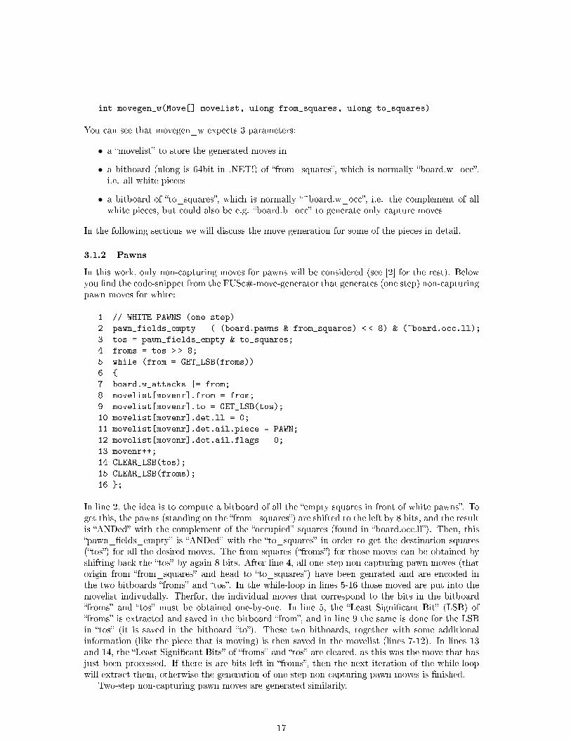
int movegen_w(Move[] movelist, ulong from_squares, ulong to_squares)
You can see that movegen_w expects 3 parameters:
• a �movelist� to store the generated moves in
• a bitboard (ulong is 64bit in .NET!) of �from_squares�, which is normally �board.w_occ�,i.e. all white pieces
• a bitboard of �to_squares�, which is normally �~board.w_occ�, i.e. the complement of allwhite pieces, but could also be e.g. �board.b_occ� to generate only capture moves
In the following sections we will discuss the move generation for some of the pieces in detail.
3.1.2 Pawns
In this work, only non-capturing moves for pawns will be considered (see [2] for the rest). Belowyou �nd the code-snippet from the FUSc#-move-generator that generates (one step) non-capturingpawn moves for white:
1 // WHITE PAWNS (one step)
2 pawn_fields_empty = ( (board.pawns & from_squares) < < 8) & (~board.occ.ll);
3 tos = pawn_fields_empty & to_squares;
4 froms = tos > > 8;
5 while (from = GET_LSB(froms))
6 {
7 board.w_attacks |= from;
8 movelist[movenr].from = from;
9 movelist[movenr].to = GET_LSB(tos);
10 movelist[movenr].det.ll = 0;
11 movelist[movenr].det.ail.piece = PAWN;
12 movelist[movenr].det.ail.flags = 0;
13 movenr++;
14 CLEAR_LSB(tos);
15 CLEAR_LSB(froms);
16 };
In line 2, the idea is to compute a bitboard of all the �empty squares in front of white pawns�. Toget this, the pawns (standing on the �from_squares�) are shifted to the left by 8 bits, and the resultis �ANDed� with the complement of the �occupied� squares (found in �board.occ.ll�). Then, this�pawn_�elds_empty� is �ANDed� with the �to_squares� in order to get the destination squares(�tos�) for all the desired moves. The from-squares (�froms�) for those moves can be obtained byshifting back the �tos� by again 8 bits. After line 4, all one-step non-capturing pawn moves (thatorigin from �from_squares� and head to �to_squares�) have been genrated and are encoded inthe two bitboards �froms� and �tos�. In the while-loop in lines 5-16 those moved are put into themovelist indivudally. Therfor, the individual moves that correspond to the bits in the bitboard�froms� and �tos� must be obtained one-by-one. In line 5, the �Least Signi�cant Bit� (LSB) of�froms� is extracted and saved in the bitboard �from�, and in line 9 the same is done for the LSBin �tos� (it is saved in the bitboard �to�). These two bitboards, together with some additionalinformation (like the piece that is moving) is then saved in the movelist (lines 7-12). In lines 13and 14, the �Least Signi�cant Bits� of �froms� and �tos� are cleared, as this was the move that hasjust been processed. If there is are bits left in �froms�, then the next iteration of the while-loopwill extract them, otherwise the generation of one-step non-capturing pawn moves is �nished.
Two-step non-capturing pawn moves are generated similarily.
17
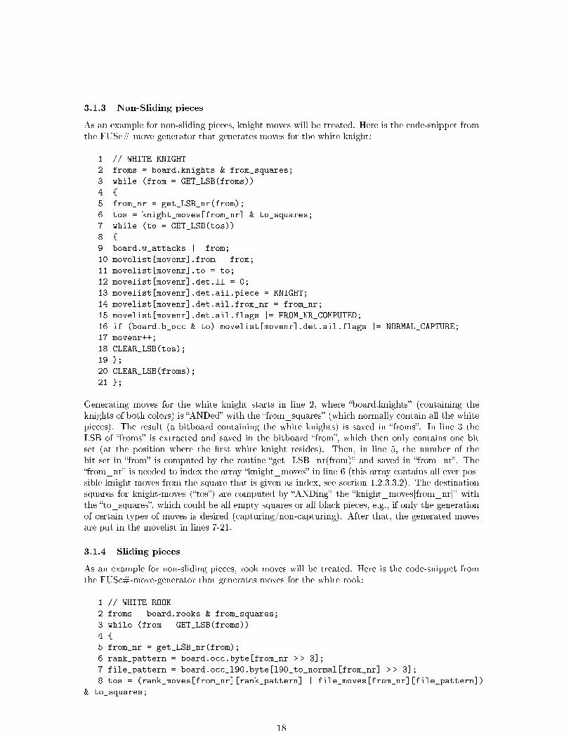
3.1.3 Non-Sliding pieces
As an example for non-sliding pieces, knight moves will be treated. Here is the code-snippet fromthe FUSc#-move-generator that generates moves for the white knight:
1 // WHITE KNIGHT
2 froms = board.knights & from_squares;
3 while (from = GET_LSB(froms))
4 {
5 from_nr = get_LSB_nr(from);
6 tos = knight_moves[from_nr] & to_squares;
7 while (to = GET_LSB(tos))
8 {
9 board.w_attacks |= from;
10 movelist[movenr].from = from;
11 movelist[movenr].to = to;
12 movelist[movenr].det.ll = 0;
13 movelist[movenr].det.ail.piece = KNIGHT;
14 movelist[movenr].det.ail.from_nr = from_nr;
15 movelist[movenr].det.ail.flags |= FROM_NR_COMPUTED;
16 if (board.b_occ & to) movelist[movenr].det.ail.flags |= NORMAL_CAPTURE;
17 movenr++;
18 CLEAR_LSB(tos);
19 };
20 CLEAR_LSB(froms);
21 };
Generating moves for the white knight starts in line 2, where �board.knights� (containing theknights of both colors) is �ANDed� with the �from_squares� (which normally contain all the whitepieces). The result (a bitboard containing the white knights) is saved in �froms�. In line 3 theLSB of �froms� is extracted and saved in the bitboard �from�, which then only contains one bitset (at the position where the �rst white knight resides). Then, in line 5, the number of thebit set in �from� is computed by the routine �get_LSB_nr(from)� and saved in �from_nr�. The�from_nr� is needed to index the array �knight_moves� in line 6 (this array contains all ever pos-sible knight moves from the square that is given as index, see section 1.2.3.3.2). The destinationsquares for knight-moves (�tos�) are computed by �ANDing� the �knight_moves[from_nr]� withthe �to_squares�, which could be all empty squares or all black pieces, e.g., if only the generationof certain types of moves is desired (capturing/non-capturing). After that, the generated movesare put in the movelist in lines 7-21.
3.1.4 Sliding pieces
As an example for non-sliding pieces, rook moves will be treated. Here is the code-snippet fromthe FUSc#-move-generator that generates moves for the white rook:
1 // WHITE ROOK
2 froms = board.rooks & from_squares;
3 while (from = GET_LSB(froms))
4 {
5 from_nr = get_LSB_nr(from);
6 rank_pattern = board.occ.byte[from_nr > > 3];
7 file_pattern = board.occ_l90.byte[l90_to_normal[from_nr] > > 3];
8 tos = (rank_moves[from_nr][rank_pattern] | file_moves[from_nr][file_pattern])
& to_squares;
18
9 while (to = GET_LSB(tos))
10 {
11 board.w_attacks |= from;
12 movelist[movenr].from = from;
13 movelist[movenr].to = to;
14 movelist[movenr].det.ll = 0;
15 movelist[movenr].det.ail.piece = ROOK;
16 movelist[movenr].det.ail.from_nr = from_nr;
17 movelist[movenr].det.ail.flags |= FROM_NR_COMPUTED;
18 if (board.b_occ & to) movelist[movenr].det.ail.flags |= NORMAL_CAPTURE;
19 movenr++;
20 CLEAR_LSB(tos);
21 };
22 CLEAR_LSB(froms);
23 };
For generating rook-moves, the idea of �rotated biboards� (section 1.2.3.3.4) comes into play. Butat �rst, the white rooks are computed and extracted in lines 2-3, and the number of the squarewhere the rook is standing is computed is line 5 and stored in �from_nr� (see previous sectionsfor details). In lines 5 and 6 patterns of the rank and the �le on which the rook is standing issaved in �rank_pattern� and ��le_pattern� respectively. These patterns are 8-bit variables thatare used to index the �rank_moves� and ��le_moves�-arrays in line 8, in addition to �from_nr�,containing the square where the rook is standing (see section 1.2.3.3.3 for details). In line 7, youcan see how the idea of accessing the �rotated� representations of the occupied squares works inpractice: The desired �le-pattern is found in
�board.occ_l90.byte[l90_to_normal[from_nr] > > 3]�
Let's look at the individual parts of this expression:
• �board.occ_l90� contains a bitboard of the occupied squares, shifted by 90◦ to the left
• this bitboard consists of 8 bytes (i.e. 64bits), that can be accessed individually by �board.occ_l90.byte[0]�to �board.occ_l90.byte[7]�
• in order to get the correct byte-number, the �from_nr� is converted to the �l90�-square-nrby accessing the array �l90_to_normal� with index �from_nr� and shifted to the right by 3bits
• this last shift can also be seen in line 6. When shifting �from_nr� (a number from 0...63) tothe right by 3 bits, you will get the number of the byte where the bit corresponding to the�from_nr� resides
Thus, after line 6 and 7, you have the correct patterns stored in �rank_pattern� and ��le_pattern�.These are used to access the pre-computed �rank_moves� and ��le_moves� arrays in line 8, wherethe bitboard of the possible destination squares for rook-moves (�tos�) is computed. The individualmoves are put in the movelist in lines 9-23 as decribed above.
3.2 Dynamic Move-Ordering in Fusc#
The current FUSc# source code contains the following dynamic move ordering heuristcs:
1. the killer heuristic
2. the history heuristic
19
3. the refutation heuristic
In this section, a brief description of the data structures used by each heuristic is given. If youare interested in more detials about these heuristics, e.g. how they are updated when a cuto�occurs, or in understanding the procedure of applying each of the heuristics to concretely sortthe generated moves inside the search algorithm, please have a look at the FUSc#-source-codeyourself, as describing the steps involved in a line-by-line fashion would go beyond the scope ofthis work.
3.2.1 Killer Heuristic
There exists two versions of the killer-heuristic in FUSc#: the �simple killer heuristic� and the�advanced killer heuristic� (see section 2.5.2).
3.2.1.1 Simple Killer Heuristic The simple killer heuristic maintains 2 killer moves for eachply, and saves a counter for both of them. Here is the appropriate data structure used in FUSc#:
public struct KillerMove
{
public Move killer1;
public sbyte counter1;
public Move killer2;
public sbyte counter2;
}
KillerMove[] s_killer_at_ply = new KillerMove[DFConstants.MAXDEPTH];
As an example, s_killer_at_ply[5].killer1 contains the �rst killer move at ply 5. Each time acuto� occurs, the cuto�-move will be compared to the killer moves: if it corresponds to one ofthem, then the respective counter is incremented, if is not among them, then the killer-move withthe lower counter is replaced by the cuto�-move.
3.2.1.2 Advanced Killer Heuristic The advanced killer heuristic uses the same data-structureas the simple killer heuristic to save 2 killer moves for each ply. However, additionally, a �killer-value� for each move is maintained, indexed by the �from� and the �to�-square (comparable to theway the �history-value� maintained for the history-heuristic, see below)
int[�] s_killer_value = new int[200,64,64];
The killer-value of a move is stored in �s_killer_value[depth,from,to]� and is incremented eachtime a cuto� occurs for the move causing the cufo�. Therfor, the search keeps track in detail howoften each move has caused a cuto� at a certain ply. This is more advanced than just maintainingcounters for the two most frequent cuto�-moves that are saved as killer-moves in the simple killerheuristic (in the simple case, also the value of the counter for a killer-move is lost as soon as themove is replaced. This can lead to a situation where a very good killer move is still replaced fre-quently, because the simple killer heuristic has no way of saving �globally� how often each move hasalready caused a cuto� for each depth. This is exactly the idea behind the �s_killer_value�-arrayin the advanced killer heuristic).
3.2.2 History Heuristic
The data structures for the history heuristic are the following:
public struct HistoryMove
20
{
public Move history1;
public sbyte value1;
public Move history2;
public sbyte value2;
}
HistoryMove s_global_history;
// the history-value of a move is stored in s_history_value[from,to]
int[,] s_history_value = new int[64,64];
Unlike the killer-heuristics described above, the history-heuristic does not maintain historymoves for each ply, but does save �global� history moves for the whole search tree. A �history-value� is maintained for each move in an array indexed by the �from� and the �to�-square. Thishistory-value is augmented each time a cuto� occurs for the move causing the cuto� (see 2.5.3 fordetails).
3.2.3 Refutation Heuristic
For the refutation heuristic, the following data-structures are maintained during the search:
public struct RefutationMove
{
public Move move;
public bool exists;
};
RefutationMove[,] s_refutation = new RefutationMove[64,64];
Each time a cuto� occurs, the cuto�-move is saved as refutation of the move the opponent haddone before. For this move, that was done before by the opponent, the �ag �exists� is set to true,so that the refutation can be tried the next time the move occurs somewhere else in the searchtree.
4 Practical Experiments with FUSc#
4.1 Verifying the Move-Generator of Fusc#
Constructing a basic move-generator is not too hard, since the basic rules for piece-movementsin chess are manageable both in number and complexity. However, when also considering specialmoves like castling, promotion and en-passent and the huge number of possible chess positionsthere are some really tricky cases to handle - and the question arises how to make sure that themove-generator of one's chess program works 100% correct, even in awkward and seldom ocurringyet possible positions. �Manually� checking the move-lists of the program is possible for only a verylimited number of positions - nevertheless it should of course be done in the process of developinga chess program, although it can always only be a �rst step. A more advanced method to verifythe move-generator of a chess engine have been developed is to use the command �perft�.
4.1.1 The �perft�-Idea
The basic idea is to implement a �perft�-command to the chess engine which will construct aminmax-tree untill a �xed depth and count all the generated nodes. This number can be comparedto the number of nodes generated by the �perft�-command of other chess engines, and there
21
exist Web-Sites with both a collection of chess positions and the corresponding correct �perft�-numbers for several depths (see [11]). Of course, special attention should be given to positionsinvolving �special moves� like castling, en-passent and promotion. One important point is that thesearch conducted by the �perft�-command must construct a plain minmax-tree without alpha-beta,transpositions tables, quiescence search, search extensions or any forward pruning techniques likenull-moves.
4.1.2 Test Positions
4.1.2.1 The Start Postion The correct results for the �perft�-command at the start positionare given in the following table. It is clear that for depth 1 (i.e. �move generation for white andcounting the nodes�) the result is 20, as there are 20 legalmoves for white in the start position inchess:
Depth Perft(Depth)
1 202 4003 8,9024 197,2815 4,865,6096 119,060,3247 3,195,901,8608 84,998,978,9569 2,439,530,234,16710 69,352,859,712,417
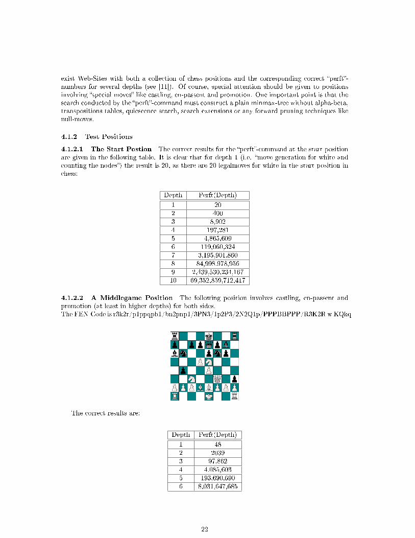
4.1.2.2 A Middlegame Position The following position involves castling, en-passent andpromotion (at least in higher depths) for both sides.The FEN-Code is r3k2r/p1ppqpb1/bn2pnp1/3PN3/1p2P3/2N2Q1p/PPPBBPPP/R3K2R w KQkq-
The correct results are:
Depth Perft(Depth)
1 482 20393 97,8624 4,085,6035 193,690,6906 8,031,647,685
22
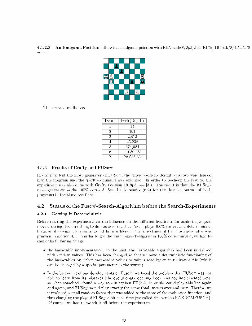
4.1.2.3 An Endgame Position Here is an endgame-poistion with FEN-code 8/2p5/3p4/KP5r/1R3p1k/8/4P1P1/8w - -
The correct results are:
Depth Perft(Depth)
1 142 1913 2,8124 43,2385 674,6246 11,030,0837 178,633,661
4.1.3 Results of Crafty and FUSc#
In order to test the move-generator of FUSc#, the three positions described above were loadedinto the program and the �perft�-command was executed. In order to re-check the results, theexperiment was also done with Crafty (version 1919p3, see [3]). The result is that the FUSc#-move-generator works 100% correct! See the Appendix (6.2) for the detailed output of bothprograms in the three positions.
4.2 Status of the Fusc#-Search-Algorithm before the Search-Experiments
4.2.1 Getting it Deterministic
Before starting the experiments on the in�uence on the di�erent heuristics for achieving a goodmove ordering, the �rst thing to do was assuring that Fusc# plays 100% correct and deterministic,because otherwise, the results would be worthless. The correctness of the move generator wasprooven in section 4.1. In order to get the Fusc#-search-algorithm 100% deterministic, we had tocheck the following things:
• the hash-table implementation: in the past, the hash-table algorithm had been initializedwith random values. This has been changed so that we have a deterministic functioning ofthe hash-tables by either hard-coded values or values read by an initialization �le (whichcan be changed by a special parameter in the source)
• In the beginning of our developments on Fusc#, we faced the problem that FUSc# was notable to learn from its mistakes (the evolutionary opening book was not implemented yet),so when somebody found a way to win against FUSc#, he or she could play this line againand again, and FUSc# would play exactly the same (bad) moves over and over. Therfor, weintroduced a small random factor that was added to the score of the evaluation function, andthus changing the play of FUSc# a bit each time (we called this version RANDOMFUSC#).Of course, we had to switch it o� before the experiments.
23
• the heuristics that we implemented for dynamic move-ordering have to be cleared every timebefore a search, so that no �old values� in�uence the search
In the end we could observe a 100% deterministic behaviour of the search of FUSc#.
4.2.2 Introducing a Framework for Conducting the Experiments
4.2.2.1 New Commands for an Automated Performing of the Tests In order to runautomated tests, several new commands were introduced to FUSc#. They can be entered directlyat the command prompt after FUSc# when started from the command-line. Normally, the en-gine understands only UCI6-commands, but for debugging and testing purposes, some additionalcommands were implemented. All of these start with �debug�, one example is �debug board�,which displays the current con�guration of the boards, or �debug boards�, which displays someof the bitboards that are used internally for board representation (see 1.2.3.2). A complete listof these additional commands can be obtained with �debug help�. In the course of this work, weimplemented the following new commands:
• �debug searchpositions positions.fen depth� starts a search on each of the positions containedin the �le �positions.fen� to a �xed depth that is passed as second parameter. The positionsmust be given in the by their FEN-codes, a standard format for describing chess positions.
• �debug test�le commands.txt� passes the commands that are stored in the �le �commands.txt�to the FUSc#-engine. Additionally, we implemented the possibility to specify a �le withcommands in the command line, e.g. by typing �Fusch commands.txt�.
• �debug loadparams params.txt� loads the engine-parameters speci�ed in the �le �params.txt�(e.g. speci�c heuristics can be turned on/o�), and thus con�gures the engine according tothese parameters
4.2.2.2 Batch-Mode and Machine-Readable Output In order to do an automated testingof the FUSc# search algorithm based on the newly commands described above, it was necessaryto implement a new special playing-mode we called �BatchMode� which should be set active whenFUSc# is called not for normal game-playing purposes but for automated testing, e.g. froma Batch-�le. The Batch-Mode assures absolute deterministic playing (see above), and disablesunwanted features like e.g. pondering that are not useful when running automated tests. Asecond extension was a parameter de�ning if FUSc# should format its output in the normalhuman-readable manner, or rather in a �MachineReadable�-manner that can be better processedfurther when doing some test series. If the �MachineOutput�-parameter is set to �true�, thenFUSc# will only output the current search depth and the number of nodes searched in a csv7-likenotation. This is much easier to process (e.g. for visualization of the data) than trying to parsethe output that FUSc# generates when playing �normally�.
4.2.3 Move Ordering in DarkFusc# 0.9
DarkFusc# 0.9 had only some very basic move ordering implemented, based on the transpositiontables and static piece-square tables8. As shown in section 2.4, the move-ordering has a greatin�uence on the e�ciency of alpha-beta searches. The aim of our experiments was thus to im-plement more sophisticated heuristics for move-ordering (like killer-moves etc.) and to test whichcombination and priority of those heuristics prooves to be most successful in achieving the smallesttree in typical ches positions.
6�unversal chess interface�, the standard protocol for communicating with a chess engine and the successor ofthe older �winboard�-protocol
7csv (�comma seperated values�) is a standard for encoding tables and data in a very simple form and can beread and written by Mircosoft Excel, e.g.
8In the terminology used later in this section, the e�ciency of the move-ordering of the old FUSc# was probablysomewhere between the �static� and the �static+TT� version, as we did also major improvements to the static moveordering in the course of this work.
24
4.3 Measuring the In�uence of the Di�erent Heuristics
The following dynamic move ordering heuristcs have been implemented in the course of this work:
1. the killer heuristic
2. the history heuristic
3. the refutation heuristic
In this section, we descibe the experiments that were conducted in order to verify that the heuristicswork correctly. An explaination of the theory behind it is given in section 2.5. For an explanationof the concrete implementation in FUSc# please refer to section 3.2.
4.3.1 General Experimental Setup
In order to gain some insights in how far the heuristics we implemented serve the goal of reducingthe number of nodes that need to be searched, a number of �xed-depths searches were conductedby FUSc# in di�erent positions, with the relevant heuristics beeing tuned on/o� indivdually.Thus, what we did was basically counting nodes for di�erent versions of FUSc# searching thesame positions. This has a clear advantage: the results can be obtained without the need toevaluate if the �chess playing strength� of FUSc# got better or worse with the introduction of anew heuristic, which is much more di�cult than just counting nodes.
Another question was whether to use the FUSc# search algorithm as it is used in normal games,or whether to modify/change it for the experiment. The second option would allow to do somemodi�cations with the aim of getting clearer results by eliminating some parts of the complex setof functional units inside a chess programm that a�ect the performance of the engine. One optionwould be, for example, to reduce the evaluation function to evaluating just the material on theboard, as this would save much time during the experiments, and one could argue that we are nottrying to tune or modify the evaluation function in these experiments anyway, so there is no harmin disabling it. But the problem is that because of the complexity of the process, the side-e�ectsof parts like e.g. the move-ordering-heuristics are not always clear: what if a heuristic that is bestfor the �material-only�-case performs signi�cantly worse compared to the others when the normal(slower) evaluation function is used, e.g. because the information gained by a more �ne-grainedevaluation can be used better by another heuristic? That's why we decided in favour of the �rstoption, i.e. to run the tests with the unmodi�ed search-algorithm that is used for normal play.This assures that the heuristics presented here work in practice, i.e. the improvements we achievedare not only valid in the �testing world�, but did improve the search (and thus the playing strength)of the FUSc# chess program in real life.
All the experiments were done workstation featuring an AMD Athlon 64 processor9, wherean evaluation copy of �Microsoft Windows XP Professional x64 Edition� was installed in orderto test if FUSc# would pro�t from a native 64bit enviroment10. And indeed, the �nodes persecond� (nps) were 2-3 higher when FUSc# was running on the 64bit platform than when runningthe same program on the same computer, but on a 32bit version of �Windows XP Professional�.The reason for this lies in the bitboard-representation that is used for the board-representation inFUSc#, which heavily relies on 64bit-operations (see section 1.2.3.2).
4.3.2 Experiment 1
The aim of our �rst experiment was to evaluate the performance of the di�erent move-orderingheuristics compared to a version of FUSc# that uses no move-ordering at all. A di�culty that
9Here is the exact hardware con�guration used: AMD Athlon 64 3000+, 1024MB DDR-Ram, 2 x 200GB MaxtorHard Discs (RAID 0), GeForce 6600 Graphics Adaptor
10In order to achieve a 64bit native runtime enviroment for FUSc#, also a 64bit version of the .NET-Framework(we used .NET 2.0 Beta 2) has to be installed. The source was compiled with �Visual Studio 2005 Beta 2� with�x64� as target platform
25

showed up in setting up the experiments is the following: there is an extreme di�erence in perfor-mance between the di�erent versions (especially between the �no-heuristics-at-all and the �best�-version). And according to the theoretical results in 2.4, this di�erence gets even much larger withhigher search dephts. Thus, a comparison with the �no-sort�-version was only possible in relativelysmall seach depths. For a comparison of the di�erent heuristics among each other, however, wewere able to reach much higher depths in our experiments (see 4.3.3).
4.3.2.1 Questions to be Answered As we described in section 3.2, we have implementedseveral move-ordering-heuristics in FUSc#, some of which were already described in the literature,but for others, to our knowledge, this has not been the case. Consequently, the main question wasof course in how far those heuristics are useful to reduce the tree size of an alpha-beta-search.
4.3.2.2 Experimental Setup A set of test positions was chosen: the LCT-II-Test11. Itcontains 35 positions, ranging from the early middlegame to the endgame taken from real games.In �Experiment 1�, we compared the following versions of FUSc#:
1. �no-sort�, with all move-ordering heuristics turned o�
2. �static�, with static move-ordering, but all dynamic move-ordering heuristics turned o�
3. �static+TT�, with static move-ordering plus the move from the Transposition Table (if avail-able)
4. �refuation�, which equals version �3.�, plus the refutation heuristic (it should actually becalled �static+TT+refutation�)
5. �history�, with the history-heuristic turned on (i.e. �static+TT+history�)
6. �killer�, with the killer-heuristic12 turned on (i.e. �static+TT+killer�)
7. �all�, with all the heuristics combined (i.e. �static+TT+refutation+history+killer�)
4.3.2.3 Results Here is the diagram of the results:
11The LCT-II-Test is a widely used test suite inside the computer chess community for testing the strength ofchess programs
12the killer-heuristic used in this experiment is actually the �killer-advanced� version. However, in this �rstexperiment we did not aim at comparing the two versions of the killer-heristic we implemented in FUSc#, this wasdone later in �Experiment 2�
26
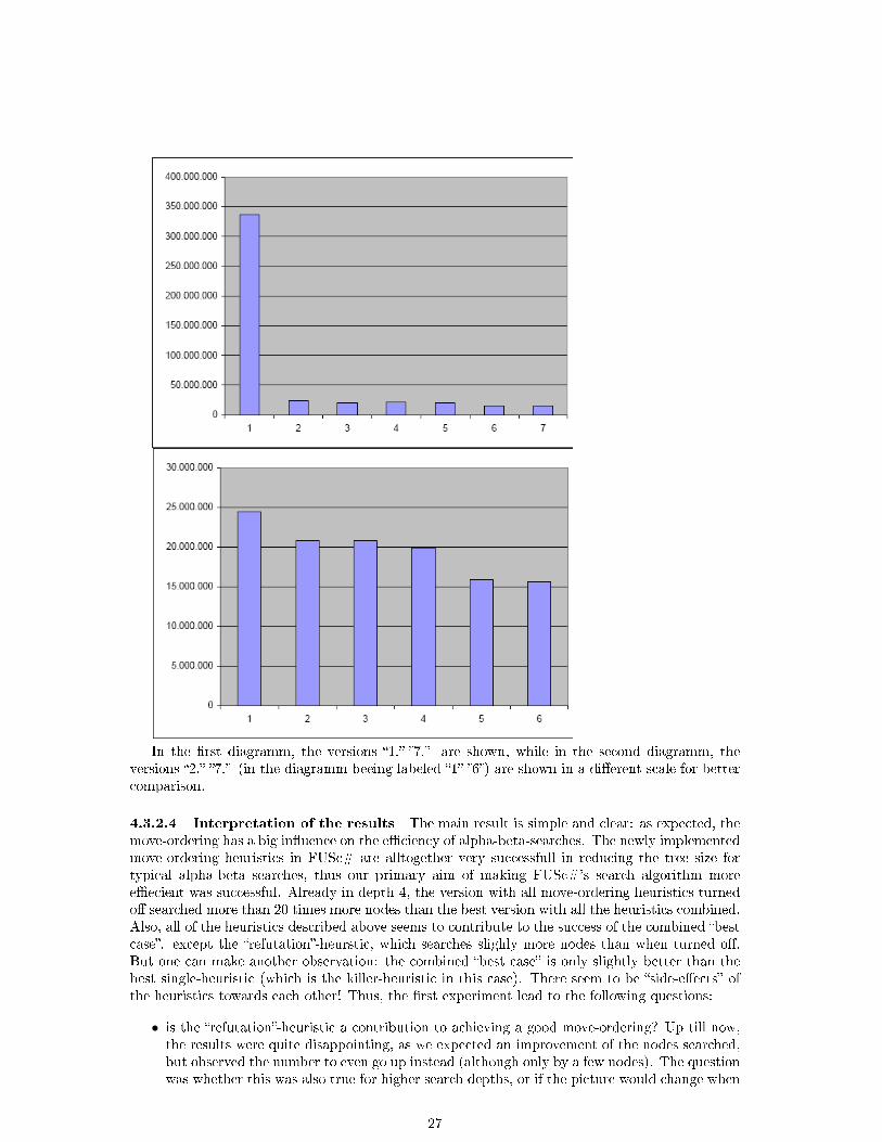
In the �rst diagramm, the versions �1.�-�7.� are shown, while in the second diagramm, theversions �2.�-�7.� (in the diagramm beeing labeled �1�-�6�) are shown in a di�erent scale for bettercomparison.
4.3.2.4 Interpretation of the results The main result is simple and clear: as expected, themove-ordering has a big in�uence on the e�ciency of alpha-beta-searches. The newly implementedmove-ordering heuristics in FUSc# are alltogether very successfull in reducing the tree size fortypical alpha-beta searches, thus our primary aim of making FUSc#'s search algorithm moree�ecient was successful. Already in depth 4, the version with all move-ordering heuristics turnedo� searched more than 20 times more nodes than the best version with all the heuristics combined.Also, all of the heuristics described above seems to contribute to the success of the combined �bestcase�. except the �refutation�-heurstic, which searches slighly more nodes than when turned o�.But one can make another observation: the combined �best case� is only slightly better than thebest single-heuristic (which is the killer-heuristic in this case). There seem to be �side-e�ects� ofthe heuristics towards each other! Thus, the �rst experiment lead to the following questions:
• is the �refutation�-heuristic a contribution to achieving a good move-ordering? Up till now,the results were quite disappointing, as we expected an improvement of the nodes searched,but observed the number to even go up instead (although only by a few nodes). The questionwas whether this was also true for higher search depths, or if the picture would change when
27
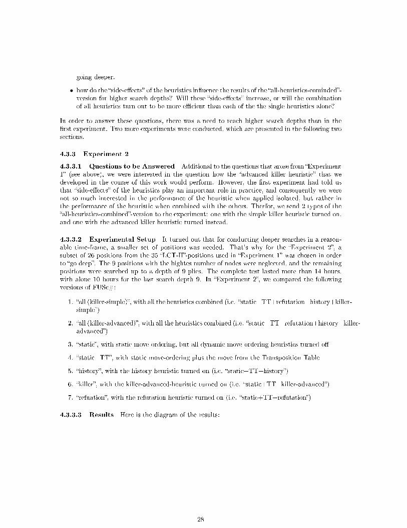
going deeper.
• how do the �side-e�ects� of the heuristics in�uence the results of the �all-heuristics-cominded�-version for higher search depths? Will these �side-e�ects� increase, or will the combinationof all heuristics turn out to be more e�cient than each of the the single heuristics alone?
In order to answer these questions, there was a need to reach higher search depths than in the�rst experiment. Two more experiments were conducted, which are presented in the following twosections.
4.3.3 Experiment 2
4.3.3.1 Questions to be Answered Additional to the questions that arose from �Experiment1� (see above), we were interested in the question how the �advanced killer heuristic� that wedeveloped in the course of this work would perform. However, the �rst experiment had told usthat �side-e�ects� of the heuristics play an important role in practice, and consequently we werenot so much interested in the performance of the heuristic when applied isolated, but rather inthe performance of the heuristic when combined with the others. Therfor, we send 2 types of the�all-heuristics-combined�-version to the experiment: one with the simple killer heuristic turned on,and one with the advanced killer heuristic turned instead.
4.3.3.2 Experimental Setup It turned out that for conducting deeper searches in a reason-able time-frame, a smaller set of positions was needed. That's why for the �Experiment 2�, asubset of 26 positions from the 35 �LCT-II�-positions used in �Experiment 1� was chosen in orderto �go deep�. The 9 positions with the hightes number of nodes were neglected, and the remainingpositions were searched up to a depth of 9 plies. The complete test lasted more than 14 hours,with alone 10 hours for the last search depth 9. In �Experiment 2�, we compared the followingversions of FUSc#:
1. �all (killer-simple)�, with all the heuristics combined (i.e. �static+TT+refutation+history+killer-simple�)
2. �all (killer-advanced)�, with all the heuristics combined (i.e. �static+TT+refutation+history+killer-advanced�)
3. �static�, with static move-ordering, but all dynamic move-ordering heuristics turned o�
4. �static+TT�, with static move-ordering plus the move from the Transposition Table
5. �history�, with the history-heuristic turned on (i.e. �static+TT+history�)
6. �killer�, with the killer-advanced-heuristic turned on (i.e. �static+TT+killer-advanced�)
7. �refuation�, with the refutation-heuristic turned on (i.e. �static+TT+refutation�)
4.3.3.3 Results Here is the diagram of the results:
28
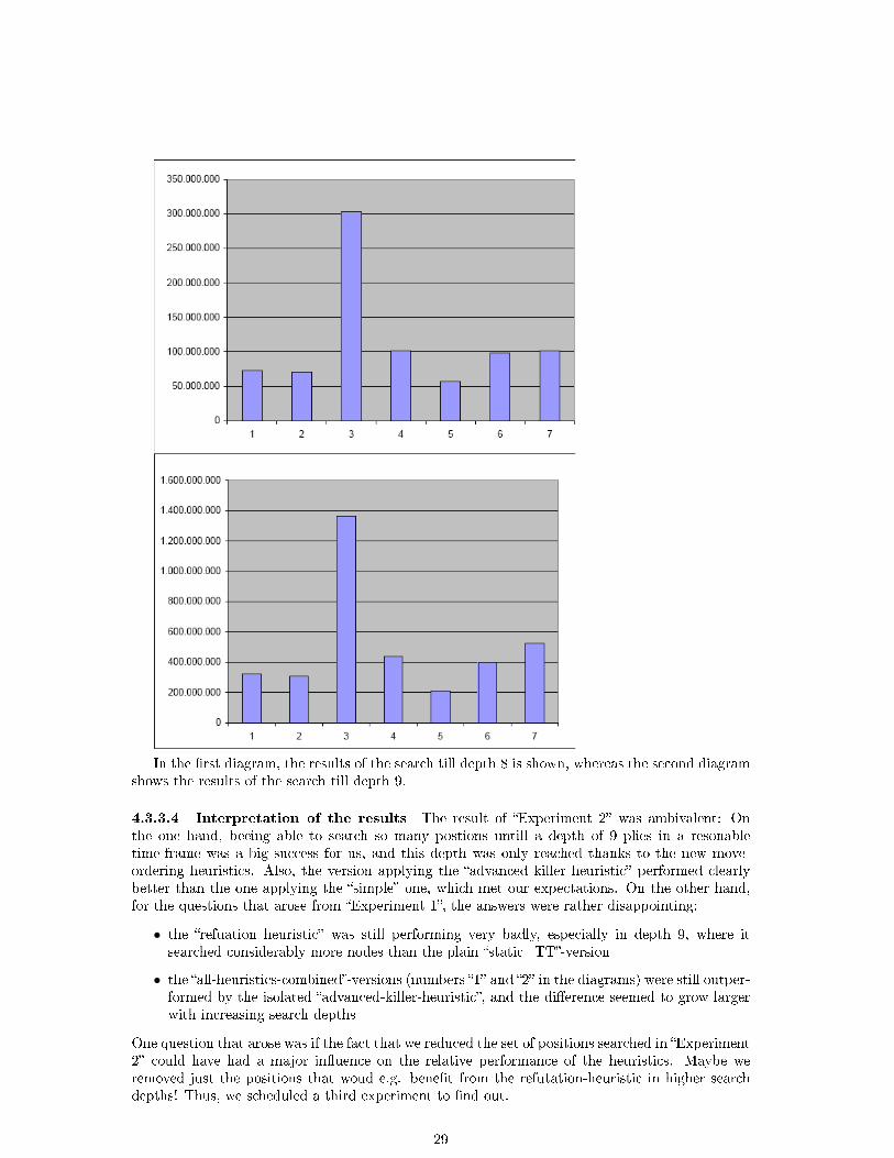
In the �rst diagram, the results of the search till depth 8 is shown, whereas the second diagramshows the results of the search till depth 9.
4.3.3.4 Interpretation of the results The result of �Experiment 2� was ambivalent: Onthe one hand, beeing able to search so many postions untill a depth of 9 plies in a resonabletime-frame was a big success for us, and this depth was only reached thanks to the new move-ordering heuristics. Also, the version applying the �advanced killer heuristic� performed clearlybetter than the one applying the �simple� one, which met our expectations. On the other hand,for the questions that arose from �Experiment 1�, the answers were rather disappointing:
• the �refuation heuristic� was still performing very badly, especially in depth 9, where itsearched considerably more nodes than the plain �static+TT�-version
• the �all-heuristics-combined�-versions (numbers �1� and �2� in the diagrams) were still outper-formed by the isolated �advanced-killer-heuristic�, and the di�erence seemed to grow largerwith increasing search depths
One question that arose was if the fact that we reduced the set of positions searched in �Experiment2� could have had a major in�uence on the relative performance of the heuristics. Maybe weremoved just the positions that woud e.g. bene�t from the refutation-heuristic in higher searchdepths! Thus, we scheduled a third experiment to �nd out.
29
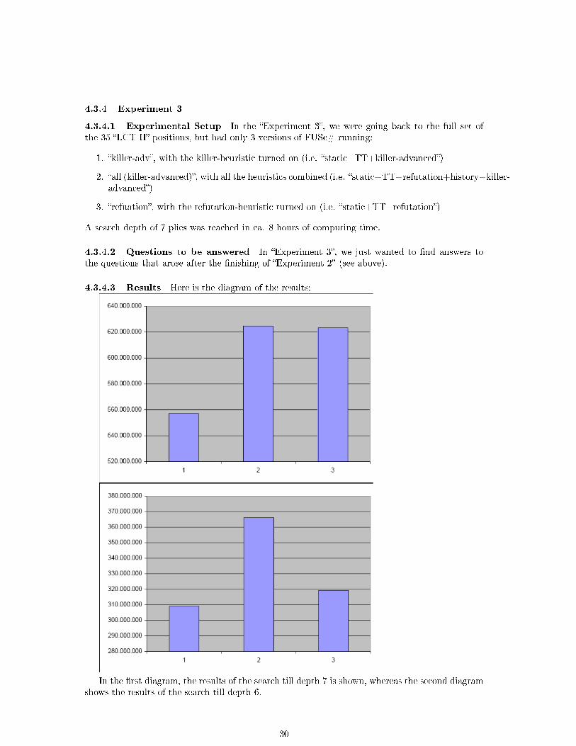
4.3.4 Experiment 3
4.3.4.1 Experimental Setup In the �Experiment 3�, we were going back to the full set ofthe 35 �LCT-II�-positions, but had only 3 versions of FUSc# running:
1. �killer-adv�, with the killer-heuristic turned on (i.e. �static+TT+killer-advanced�)
2. �all (killer-advanced)�, with all the heuristics combined (i.e. �static+TT+refutation+history+killer-advanced�)
3. �refuation�, with the refutation-heuristic turned on (i.e. �static+TT+refutation�)
A search depth of 7 plies was reached in ca. 8 hours of computing time.
4.3.4.2 Questions to be answered In �Experiment 3�, we just wanted to �nd answers tothe questions that arose after the �nishing of �Experiment 2� (see above).
4.3.4.3 Results Here is the diagram of the results:
In the �rst diagram, the results of the search till depth 7 is shown, whereas the second diagramshows the results of the search till depth 6.
30
4.3.4.4 Interpretation of the Results For the two still open questions from �Experiment2� (actually, they already arose in �Experiment 1�), we obtained the following results:
• the �refuation-heuristic� lead to a considerable reduction of the nodes searched at depth 6and a slight improvement at depth 7
• the �killer-advanced�-heuristic seems to be the best of the currently implemented move-ordering heuristics, but only when implemented isolated from the others, as there seem tobe many side-e�ects, occuring especially in higher search depths
The second point was a quite unexpected result, and needs further clari�cation (see next para-graph).
4.4 Interpretation of the Results of the three Search Experiments
The main result of our experiments is that we were successful in improving the move-orderingin FUSc#: �Experiment 1� showed that already in depth 4, the version with all move-orderingheuristics turned o� searched more than 20 times more nodes than the best version with all theheuristics combined. Also, all of the heuristics we implemented in FUSc#, when applied alone,reduce the number of nodes searched - although there are special cases where certain heuristicsfail, like e.g. the �refutation-heuristic� for smaller search depth, as we observed in �Experiment1�. But alone beeing able to search so many postions untill a depth of 9 plies in �Experiment 2�in a resonable time-frame was a big success for us, and this depth was only reached thanks to thenew move-ordering heuristics. Also, the version applying the �advanced killer heuristic� performedclearly better than the one applying the �simple� one. However, the main challenge seems to be tocontrol the �side-e�ects� that occur when the individual heuristics are combined: Our experiments2 and 3 showed that it is not always the case that the �all-heuristics-combined�-version of thealgorithm performs best, instead in our experiments the �killer-advanced�-heuristic was globallythe best when applied alone, without the others! This is a quite astonishing result, and there hasto be done further reasearch and testing in order to verify this hypothesis.
5 Conclusion/Future research
The aim of this work was to give an overview of the theory of e�cient alpha-beta-searches incomputer chess and to explain the practical strategies implemented in the FUSc# chess program.The main focus was put on two topics: the �rst one was e�cient move generation with �rotatedbitboards�, and the second one was how to carry out e�cient alpha-beta-searches by optimizingthe move-ordering with static and dynamic heuristics. Pracical experiments with FUSc# wereused to verify the theoretical results in both questions.
One of the challenges for optimizing the application of dynamic move ordering heuristics isthat the heuristics tend to perform extremly di�erent depending upon the exact conditions of theexperiment: the result will depend on the selection of positions, on the chosen search depth, andprobably on other factors that were not changed during our experiments but could as well beincluded in the set of parameters (like which variant of alpha-beta is used to perform the search,because it might be that one heuristic performs better with plain alpha-beta while beeing worsewith MTD(f), for example). Also, there are even more parameters to tune concerning the move-ordering that just switching move-ordering-heuristcs on or o�: one could �ne-tune the exact orderin which the heuristics are applied (e.g. �should the killer move come before the refutation moveor afterwards?�) or even include multiple variants of the heuristics (e.g. allowing captures in thekiller-move slots or not). Alltogether, it seems to us that manually testing all of the di�erentvariants is not desirable, as this will need extremely much time, and is basically a �try-and-error�procedure. On the contrary, the search-algorithm of FUSc# seems to be at a point where asystematic testing of all the mentioned parameters would be needed in order to �nd out the bestcombination. This could be done either by massively running tests of di�erent versions of FUSc#,
31
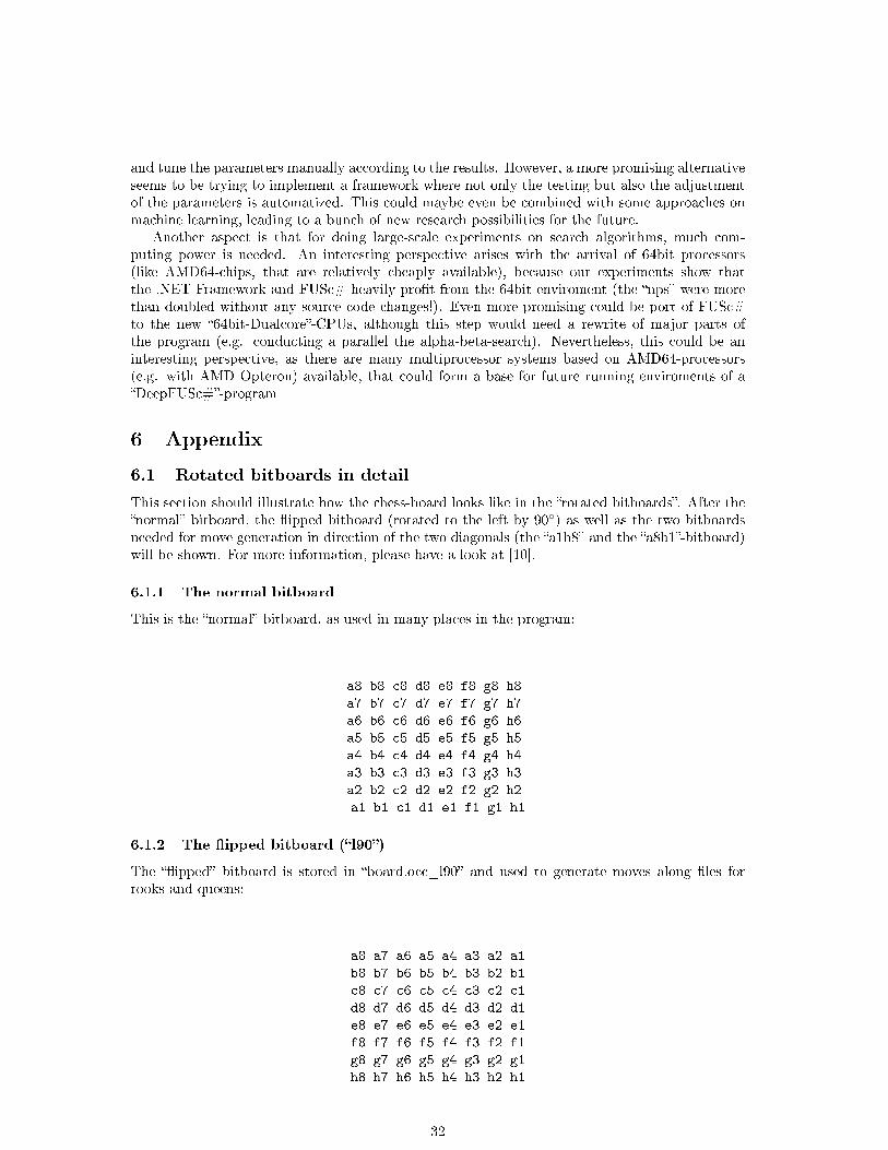
and tune the parameters manually according to the results. However, a more promising alternativeseems to be trying to implement a framework where not only the testing but also the adjustmentof the parameters is automatized. This could maybe even be combined with some approaches onmachine learning, leading to a bunch of new research possibilities for the future.
Another aspect is that for doing large-scale experiments on search algorithms, much com-puting power is needed. An interesting perspective arises with the arrival of 64bit processors(like AMD64-chips, that are relatively cheaply available), because our experiments show thatthe .NET-Framework and FUSc# heavily pro�t from the 64bit enviroment (the �nps� were morethan doubled without any source code changes!). Even more promising could be port of FUSc#to the new �64bit-Dualcore�-CPUs, although this step would need a rewrite of major parts ofthe program (e.g. conducting a parallel the alpha-beta-search). Nevertheless, this could be aninteresting perspective, as there are many multiprocessor systems based on AMD64-processors(e.g. with AMD Opteron) available, that could form a base for future running enviroments of a�DeepFUSc#�-program
6 Appendix
6.1 Rotated bitboards in detail
This section should illustrate how the chess-board looks like in the �rotated bitboards�. After the�normal� bitboard, the �ipped bitboard (rotated to the left by 90◦) as well as the two bitboardsneeded for move generation in direction of the two diagonals (the �a1h8� and the �a8h1�-bitboard)will be shown. For more information, please have a look at [10].
6.1.1 The normal bitboard
This is the �normal� bitboard, as used in many places in the program:
a8 b8 c8 d8 e8 f8 g8 h8
a7 b7 c7 d7 e7 f7 g7 h7
a6 b6 c6 d6 e6 f6 g6 h6
a5 b5 c5 d5 e5 f5 g5 h5
a4 b4 c4 d4 e4 f4 g4 h4
a3 b3 c3 d3 e3 f3 g3 h3
a2 b2 c2 d2 e2 f2 g2 h2
a1 b1 c1 d1 e1 f1 g1 h1
6.1.2 The �ipped bitboard (�l90�)
The ��ipped� bitboard is stored in �board.occ_l90� and used to generate moves along �les forrooks and queens:
a8 a7 a6 a5 a4 a3 a2 a1
b8 b7 b6 b5 b4 b3 b2 b1
c8 c7 c6 c5 c4 c3 c2 c1
d8 d7 d6 d5 d4 d3 d2 d1
e8 e7 e6 e5 e4 e3 e2 e1
f8 f7 f6 f5 f4 f3 f2 f1
g8 g7 g6 g5 g4 g3 g2 g1
h8 h7 h6 h5 h4 h3 h2 h1
32
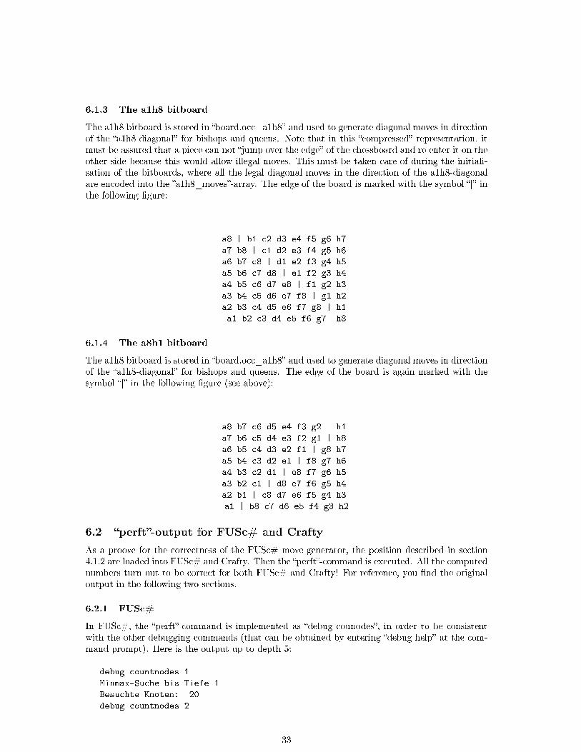
6.1.3 The a1h8 bitboard
The a1h8 bitboard is stored in �board.occ_a1h8� and used to generate diagonal moves in directionof the �a1h8-diagonal� for bishops and queens. Note that in this �compressed� representation, itmust be assured that a piece can not �jump over the edge� of the chessboard and re-enter it on theother side because this would allow illegal moves. This must be taken care of during the initiali-sation of the bitboards, where all the legal diagonal moves in the direction of the a1h8-diagonalare encoded into the �a1h8_moves�-array. The edge of the board is marked with the symbol �|� inthe following �gure:
a8 | b1 c2 d3 e4 f5 g6 h7
a7 b8 | c1 d2 e3 f4 g5 h6
a6 b7 c8 | d1 e2 f3 g4 h5
a5 b6 c7 d8 | e1 f2 g3 h4
a4 b5 c6 d7 e8 | f1 g2 h3
a3 b4 c5 d6 e7 f8 | g1 h2
a2 b3 c4 d5 e6 f7 g8 | h1
a1 b2 c3 d4 e5 f6 g7 h8
6.1.4 The a8h1 bitboard
The a1h8 bitboard is stored in �board.occ_a1h8� and used to generate diagonal moves in directionof the �a1h8-diagonal� for bishops and queens. The edge of the board is again marked with thesymbol �|� in the following �gure (see above):
a8 b7 c6 d5 e4 f3 g2 h1
a7 b6 c5 d4 e3 f2 g1 | h8
a6 b5 c4 d3 e2 f1 | g8 h7
a5 b4 c3 d2 e1 | f8 g7 h6
a4 b3 c2 d1 | e8 f7 g6 h5
a3 b2 c1 | d8 e7 f6 g5 h4
a2 b1 | c8 d7 e6 f5 g4 h3
a1 | b8 c7 d6 e5 f4 g3 h2
6.2 �perft�-output for FUSc# and Crafty
As a proove for the correctness of the FUSc# move generator, the position described in section4.1.2 are loaded into FUSc# and Crafty. Then the �perft�-command is executed. All the computednumbers turn out to be correct for both FUSc# and Crafty! For reference, you �nd the originaloutput in the following two sections.
6.2.1 FUSc#
In FUSc#, the �perft�-command is implemented as �debug counodes�, in order to be consistentwith the other debugging commands (that can be obtained by entering �debug help� at the com-mand prompt). Here is the output up to depth 5:
debug countnodes 1
Minmax-Suche bis Tiefe 1
Besuchte Knoten: 20
debug countnodes 2
33
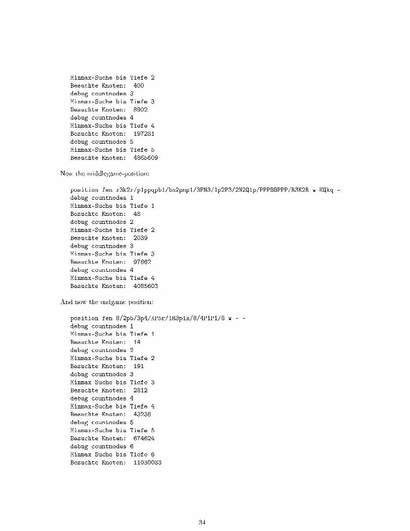
Minmax-Suche bis Tiefe 2
Besuchte Knoten: 400
debug countnodes 3
Minmax-Suche bis Tiefe 3
Besuchte Knoten: 8902
debug countnodes 4
Minmax-Suche bis Tiefe 4
Besuchte Knoten: 197281
debug countnodes 5
Minmax-Suche bis Tiefe 5
Besuchte Knoten: 4865609
Now the middlegame-position:
position fen r3k2r/p1ppqpb1/bn2pnp1/3PN3/1p2P3/2N2Q1p/PPPBBPPP/R3K2R w KQkq -
debug countnodes 1
Minmax-Suche bis Tiefe 1
Besuchte Knoten: 48
debug countnodes 2
Minmax-Suche bis Tiefe 2
Besuchte Knoten: 2039
debug countnodes 3
Minmax-Suche bis Tiefe 3
Besuchte Knoten: 97862
debug countnodes 4
Minmax-Suche bis Tiefe 4
Besuchte Knoten: 4085603
And now the endgame-position:
position fen 8/2p5/3p4/KP5r/1R3p1k/8/4P1P1/8 w - -
debug countnodes 1
Minmax-Suche bis Tiefe 1
Besuchte Knoten: 14
debug countnodes 2
Minmax-Suche bis Tiefe 2
Besuchte Knoten: 191
debug countnodes 3
Minmax-Suche bis Tiefe 3
Besuchte Knoten: 2812
debug countnodes 4
Minmax-Suche bis Tiefe 4
Besuchte Knoten: 43238
debug countnodes 5
Minmax-Suche bis Tiefe 5
Besuchte Knoten: 674624
debug countnodes 6
Minmax-Suche bis Tiefe 6
Besuchte Knoten: 11030083
34
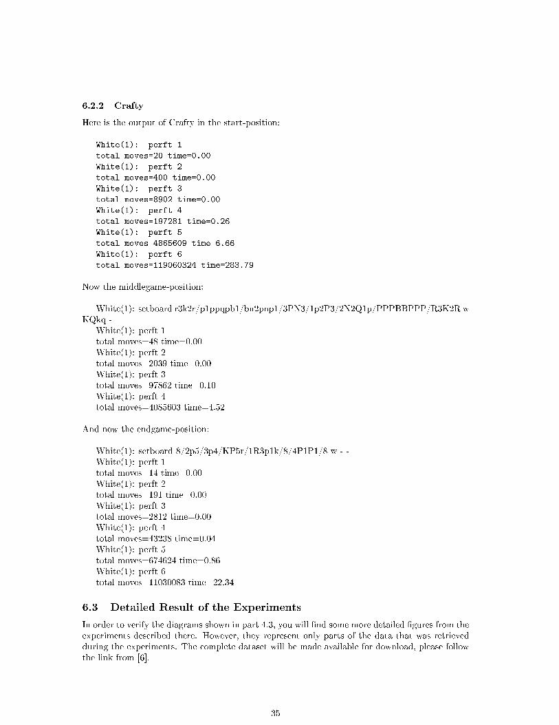
6.2.2 Crafty
Here is the output of Crafty in the start-position:
White(1): perft 1
total moves=20 time=0.00
White(1): perft 2
total moves=400 time=0.00
White(1): perft 3
total moves=8902 time=0.00
White(1): perft 4
total moves=197281 time=0.26
White(1): perft 5
total moves=4865609 time=6.66
White(1): perft 6
total moves=119060324 time=283.79
Now the middlegame-position:
White(1): setboard r3k2r/p1ppqpb1/bn2pnp1/3PN3/1p2P3/2N2Q1p/PPPBBPPP/R3K2R wKQkq -
White(1): perft 1total moves=48 time=0.00White(1): perft 2total moves=2039 time=0.00White(1): perft 3total moves=97862 time=0.10White(1): perft 4total moves=4085603 time=4.52
And now the endgame-position:
White(1): setboard 8/2p5/3p4/KP5r/1R3p1k/8/4P1P1/8 w - -White(1): perft 1total moves=14 time=0.00White(1): perft 2total moves=191 time=0.00White(1): perft 3total moves=2812 time=0.00White(1): perft 4total moves=43238 time=0.04White(1): perft 5total moves=674624 time=0.86White(1): perft 6total moves=11030083 time=22.34
6.3 Detailed Result of the Experiments
In order to verify the diagrams shown in part 4.3, you will �nd some more detailed �gures from theexperiments described there. However, they represent only parts of the data that was retrievedduring the experiments. The complete dataset will be made available for download, please followthe link from [6].
35
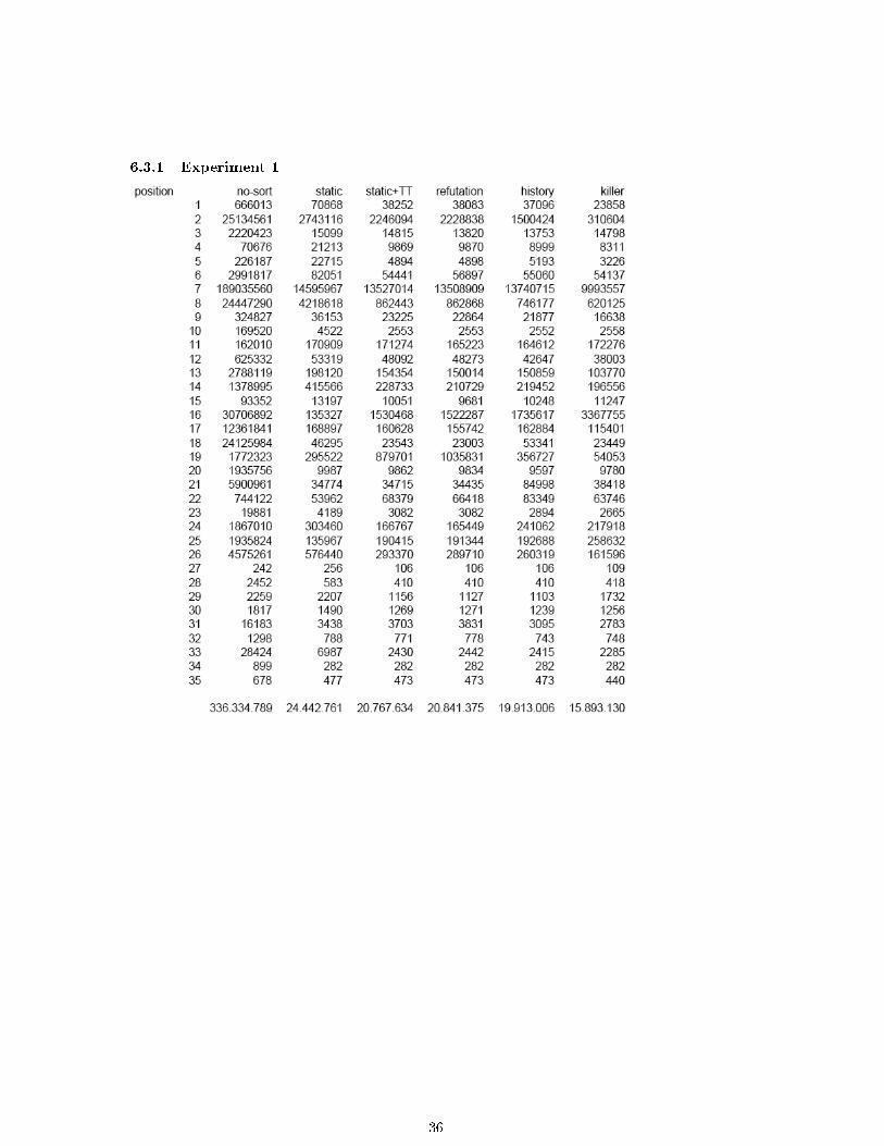
6.3.1 Experiment 1
36
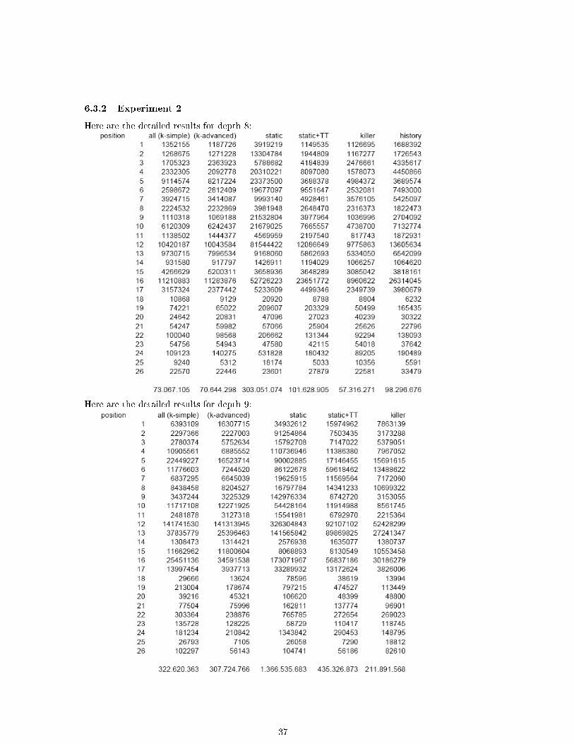
6.3.2 Experiment 2
Here are the detailed results for depth 8:
Here are the detailed results for depth 9:
37
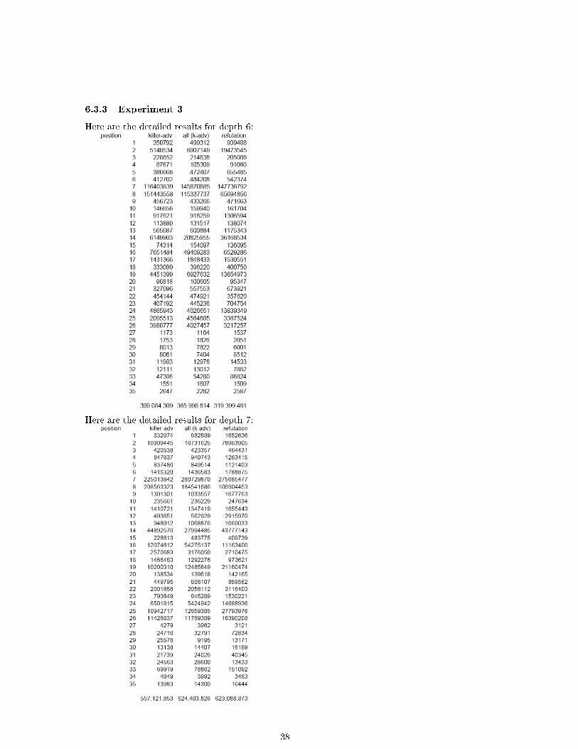
6.3.3 Experiment 3
Here are the detailed results for depth 6:
Here are the detailed results for depth 7:
38
References
[1] Block, Marco, Verwendung von Temporale-Di�erenz-Methoden im Schachmotor FUSc#,Diplomarbeit, Berlin, 2004
[2] Buchner, Johannes: Rotated Bitboards in FUSc#, Seminararbeit, Berlin, 2005
[3] Crafty-Homepage: http://www.cis.uab.edu/info/faculty/hyatt/hyatt.html
[4] Dill, Sebastian, Transpositionstabellen, Seminararbeit, Berlin, 2005
[5] Download of DarkFUSc# and FUSc#: http://page.mi.fu-berlin.de/~fusch/download/
[6] FUSc#-Homepage: http://www.fuschmotor.de.vu
[7] FUSc#-Server: http://www.inf.fu-berlin.de/~fusch/
[8] Frey, P.W. (editor), Chess skill in man and machine, Springer, 2nd edition 1983
[9] Heinz, Ernst A., Scalable search in computer chess, Vieweg, 2000
[10] Heinz, Ernst A.: How DarkThought plays chess, http://supertech.lcs.mit.edu/~heinz/dt/node2.html
[11] Homepage of Peter McKenzie on Computer chess: http://homepages.caverock.net.nz/~peter/perft.htm
[12] Homepage Microsoft .NET: http://www.microsoft.com/net/default.mspx
[13] Homepage of gcc: http://gcc.gnu.org/
[14] Kaindl, H., Tree Seaching Algorithms (chapter 8 of [17]).
[15] Luger, George F.: Arti�cial Intelligence, 2nd edition, 1993
[16] Plaat, Aske: RESEARCH, RE:SEARCH & RE-SEARCH, Tinbergen Institute, 1996
[17] T.Antony Marsland, Jonathan Schae�er (Editors), Computers, Chess and Cognition,Springer, 1990
[18] Reinefeld, Alexander, Spielbaum Suchverfahren, Informatik-Fachberichte 200, Springer Ver-lag, 1989.
[19] Shannon, Claude, Programming a Computer for Playing Chess, Philosophical Magazine,Ser.7, Vol. 41, No. 314 - March 1950.
[20] Slagle, James H. and Dixon, John K., Experiments with some programs that search gametrees, Journal of the ACM, 16(2):p.189-207, April 1969
[21] Reinefeld, Alexander, Spielbaum Suchverfahren, Informatik-Fachberichte 200, Springer Ver-lag, 1989.
[22] Stockman, George C., A minimax algorithm better than Alpha-Beta?, Arti�cial Intelligence,12(2):p179-196, 1979.
39