theory and methods for calculating the inertial …
TRANSCRIPT

Yevgeniy Kalinichenko
THEORY AND METHODS FOR CALCULATING
THE INERTIAL-BRAKING CHARACTERISTICS
OF A SHIP
Monograph
2020

UDC 629.12.073.33-56K 17
Published in 2020 by PC Technology CenterShatilova dacha str., 4, of. 702, Kharkiv, Ukraine, 61145
Approved by the Academic Council of Odessa National Maritime University, Protocol No. 5 of 23.12.2020
Reviewers:Tymoshchuk Elena, Doctor of Technical Sciences, Professor of the Department of Navigation and Shiphandling, Kyiv State Maritime Academy named after hetman Petro Konashevich, State University of Infrastructure and Technology;Varbanets Roman, Doctor of Technical Sciences, Professor, Head of the Ship Power Plants and Technical Operation Department of Odessa National Maritime University
K 17 Author:
Kalinichenko Yevgeniy
Theory and methods for calculating the inertial-braking characteristics of a ship: monograph / Y. Kalinichenko. – Kharkiv: PC Technology Center, 2020. – 76 p.
ISBN 978-617-7319-30-5 (on-line)
The monograph presents the results of a study of alternative methods for improving the quality and speed of obtaining information about the inertial-braking characteristics of a ship. The study is carried out using a methodology based on the development of theoreti-cal foundations, mathematical models and comparison of calculated characteristics with data from a full-scale experiment. The problems of calculating and formalizing the inertial-brak-ing characteristics of the ship are comprehensively solved. For the first time, to derive the calculated formulas for the time and stopping distance, theorems are used on the change in the momentum and kinetic energy during accelerated and decelerated movement of the ship, and a method is developed to take into account the influence of the passing and opponent current on the stopping distance of the ship.
The monograph is intended for scientific and pedagogical, engineering and technical personnel, ship engineering and technical personnel and graduates of navigational special-ties of maritime higher educational institutions.
Fig. 23, Tables 9, References 51 items.
DOI: 10.15587/978-617-7319-30-5
ISBN 978-617-7319-30-5 (on-line)
Copyright © 2020 Kalinichenko Yevgeniy
This tutorial is publicly available under license. CC BY http://creativecommons.org/licenses/by/4.0.
3
AUTOBIOGRAPHY
Yevgeniy KalinichenkoPhD, Master Mariner.Member of London Nautical Institute (AFNI).Member of the Maritime Institute of Ukraine.Member of the International Federation of Shipmasters’ Association.Member of the Odessa Shipmasters’ Association.
Was born on March 18, 1964 in Kharkiv City. In the same year, the family returned to Odessa, where the father lives. In 1971–1981 teaching in secondary schools of Odessa and Chorno morsk. From 1981 to 1987 cadet of the Odessa Higher Engineering Marine School. In 1987–1996, after graduating from OHEMS, he worked in the KSC and BSC as an Deck Of-ficer on ocean-going large-tonnage vessels, and since 1996 on ships of foreign ship owners as a Chief Officer and, since 2001, as a Shipmaster. In the same 2001 he began teaching at the Odessa National Maritime Academy, and then at the National University «Odessa Maritime Academy» in the Shiphandling Department. He worked as an assistant, senior lecturer and associate professor and at the same time was constantly on probation as a shipmaster on the ships of the best foreign companies: DELMAS, DOCKWISE, CMA CGM, ENESEL, MSC. He graduated from the postgraduate study of ONMA in 2009. In 2011, he studied at special courses in the shiphandling of large-capacity container ships in the Polish city of Ilawa. In the same year he was elected to the London Nautical Institute and the Maritime Institute of Ukraine. In 2017 he defended his thesis and received the de-gree of candidate of technical sciences. Since 2019, Associate Professor at Odessa National Maritime University. The general shipmaster’s and teaching experience is 19 years. He has several dozen scientific works and publications in domestic and foreign publications. He has repeatedly participated in international con ferences. Fluent in English.
«I dedicate this book to the blessed memory of my teachers: Dr. Yuriy L. Vorobyov and Capt. Petr I. Yarkin»

4
ABSTRACT
One of the most serious problems of modern navigation is the accident rate that occurs due to inept or belated maneuvering of ships. As a result of accidents in the world, more than 200 ships sink every year and every fourth receives significant damage.
Full-scale tests show that the stopping distance of large-tonnage ships turn out to be much less permissible, and shipbuilders are able to significantly reduce the astern power of such ships, making them cheaper at the expense of safety.
The low accuracy of inertial-braking characteristics is mainly due to unqualified field tests. Analysis of graphs and tables based on the results of such tests show that the spread in the values of inertial-braking characteristics for ships of the same type reaches 30%, and in some cases even more. In many tables and graphs, inertial-braking characteristics are expressed in relative values and are not suitable for direct use when maneuvering a ship. Finally, even when graphical and/or tabular maneuvering information is available on the navigating bridge, it is difficult to use it when maneuvering a ship at night.
The research carried out by the author results in:– creation of an alternative computational method for determining the iner-
tial-braking characteristics of the ship, suitable for use on any on-board computer;– development of an improved methodology for calculating the path and time of
acceleration and braking of the ship in various ahead motion modes;– development of a methodology for taking into account the influence of a passing
and opponent current on the length of the stopping distance of the ship;– development of methods for solving applied problems, ensuring a decrease in the
accident rate of ships during maneuvering.The obtained methods include the development of theoretical foundations, mathe-
matical models and comparison of the calculated inertial-braking characteristics of ships with the data of a full-scale experiment. For the first time, to derive the calculated formulas for the time and stopping distance, theorems are used on the change in the momentum and kinetic energy during accelerated and decelerated motion of the ship. In the course of the study, the problems of calculating and formalizing the inertial-braking characteristics of the ship are being comprehensively solved. For the first time, the hypothesis that the nature of the change in the thrust force of the propeller during reverse can be approximated by linear equations has been substantiated and confirmed. The general results are used to calculate the inertial-braking characteristics of specific ships.
KEYWORDS
Maneuvering of ships, accident rate, navigation safety, inertial-braking characteris-tics, full-scale tests, propeller thrust, resistance to ship movement.

5
List of Tables ...................................................................................................................7List of Figures .................................................................................................................8Introduction ....................................................................................................................9
Chapter 1 Review and analysis of literature ...........................................................11References ...............................................................................................................19
Chapter 2 Theoretical justification of the methodology of calculating
the way and time of braking of the ship ..................................................................212.1 The system of equations for the movement of the ship in the
horizontal plane .............................................................................................212.2 Derivation of design formulas for determining the stopping
length and braking time of the ship when the propeller is reversed (active braking) ..............................................................................22
2.3 Determination of the mean value of the propeller thrust .......................272.4 Determination of the exponent value a .....................................................282.5 Determination of the proportionality coefficient m............................... 292.6 Determination of the added mass coefficient k ........................................312.7 An example of calculating the length and time of stopping
distance of a ship with active braking ........................................................322.8 Determination of the length and time of stopping distance during
passive braking ..............................................................................................332.9 Example of calculating the length and time of stopping distance
for passive braking ........................................................................................35References ...............................................................................................................36
Chapter 3 Determination of the characteristics of the active ship braking.
Alternative approach ...................................................................................................373.1 Derivation of calculation formulas .............................................................383.2 Influence of passing and opponent current on the braking
length of the ship ...........................................................................................423.3 Determining the time and speed of the ship’s acceleration astern .........44References ...............................................................................................................46
Chapter 4 Determination of ship acceleration and braking characteristics .....474.1 Theoretical substantiation and derivation of calculation formulas .......48
CONTENT

Theory and methods for calculating the inertial-braking characteristics of a ship
6
4.2 The procedure for calculating the path length and acceleration and braking time for «Vasily Porik» motor ship ......................................53
References ...............................................................................................................55
Chapter 5 Practical application of inertial-braking characteristics of a ship ....565.1 Calculation of safe speed and minimum permissible distance
of ship convergence .......................................................................................565.2 Accounting for stopping distance when ships navigate in ice
behind the icebreaker ...................................................................................61References ...............................................................................................................62
Chapter 6 Practical calculation of inertial-braking characteristics for
the «ELQUI» container carrier .................................................................................646.1 Ship data .........................................................................................................646.2 Calculation of active braking characteristics ............................................656.3 Calculation of the characteristics of the ship’s acceleration from
a stationary state to the speed of full maneuvering speed ......................686.4 Calculation of the characteristics of the laden ship braking
from full maneuverability to the dead slow ahead speed ........................696.5 Calculation of the characteristics of passive braking from full
maneuvering to stop for a laden ship and ship in ballast ........................706.6 Calculation of the speed and time of acceleration of a laden ship
at full speed astern from a stationary state to a stopping distance length equal to the length of the ship’s hull ...............................................72
6.7 Representation of inertial-braking characteristics in the form of analytical dependencies ...........................................................................73
References ...............................................................................................................74
General conclusions ....................................................................................................75

7
LIST OF TABLES
3.1 Calculation of braking characteristics of the «Uelen» motor ship ...............414.1 Characteristics of acceleration and braking of the «Vasily Porik»
motor ship ............................................................................................................544.2 Acceleration from motionless state of the «Vasily Porik» motor ship .........546.1 Calculation results for a laden ship ..................................................................666.2 Calculation results for a ship in ballast ............................................................666.3 Calculation results for a laden ship ..................................................................686.4 Calculation results for a laden ship ..................................................................696.5 Calculation results for a laden ship ..................................................................706.6 Calculation results for a ship in ballast ............................................................70

8
LIST OF FIGURES
1.1 Scheme for changing the propeller thrust when reversing: a – by formula (1.5); b – according to the thrust meter ................................18
2.1 Graph of the auxiliary variable Dt for five values of the exponent «a» .......262.2 Graph of the auxiliary variable DS for six values of the exponent «a» ........272.3 Dependence of resistance on speed of 12 and 18.3 knots for a ship
with a displacement of 22100 tons ....................................................................294.1 Dependence of the propeller thrust forces and resistance to movement
on speed ................................................................................................................484.2 The nature of acceleration change .....................................................................494.3 Thrust coefficient as a function of the relative propeller pitch,
approximated by a linear relationship ..............................................................504.4 Dependence of speed on the path of acceleration and braking of
the «Vasily Porik» motor ship............................................................................544.5 Dependence of the speed on the acceleration and braking time of
the «Vasily Porik» motor ship............................................................................555.1 Influence of the radar parameter on the radius of the danger zone ............605.2 Scheme of the caravan formation .....................................................................616.1 Dependence of the active braking distance on the speed for a laden ship ....666.2 Dependence of the active braking distance on the speed for a ship
in ballast ...............................................................................................................676.3 Dependence of active braking distance on speed for a ship in ballast ........676.4 Dependence of active braking time on speed for a ship in ballast ...............676.5 Dependence of the acceleration path on the speed for the laden ship ........686.6 Dependence of acceleration time on speed for a laden ship .........................686.7 Dependence of the braking distance on speed ...............................................696.8 Dependences of braking time on speed for a laden ship ...............................696.9 Dependence of the stopping distance on the speed of passive braking
for a laden ship ....................................................................................................716.10 Dependence of time on the speed of passive braking for a laden ship .......716.11 Dependence of the path length on the passive braking speed for a ship
in ballast ................................................................................................................716.12 Dependence of time of passive braking speed for a ship in ballast .............72

9
INTRODUCTION
One of the most serious problems of modern navigation is the accident rate that occurs due to inept or belated maneuvering of ships.As a result of accidents in the world, more than 200 ships sink every year and every fourth receives signi-ficant damage. Numerous cases of collisions of ships, bulkheads on each other and on shore facilities, groundings, etc. also indicate that a significant defect of some ship complexes is the long duration of the reversing process and an unacceptably long stopping distance.
On December 5, 2002, the Maritime Safety Committee of the International Maritime Organization adopted standards for the maneuverability of trans-port ships, which would increase safety at sea and protect the marine environ-ment. However, according to these criteria, the braking distance when braking from full ahead to full astern is allowed up to 15–20 hull lengths, depending on the ship’s power-to-weight per tonne of displacement. Full-scale tests of an oil tanker with a displacement of 156,230 tons and a tanker with a displace-ment of 125,273 tons showed stopping distances for these ships, respectively, 10 and 7 hull lengths. Consequently, shipbuilders were able to significantly re-duce the reverse power of such ships, making them cheaper at the expense of reduced safety.
On the navigating bridges of many ships, information about their iner-tial-braking characteristics is either completely absent, or it is not presented fully and accurately enough. The low accuracy of inertial-braking characteristics is mainly due to unqualified field tests. Analysis of graphs and tables based on the results of such tests has been shown that the spread in the values of inertial-brak-ing characteristics for ships of the same type reaches 30 %, and in some cases even more. In many tables and graphs, inertial-braking characteristics are expressed in relative terms, for example, in hull lengths, so they are generally not suitable for direct use when maneuvering a ship.
Finally, even when graphical and/or tabular maneuvering information is available on the navigating bridge, it is difficult to use it when maneuvering a ship at night. Such information could be stored in an onboard computer connected to lag sensors, gyrocompass and other navigation devices, and continuously dis-played on the monitor screen.
The research carried out by the author resulted in:– creation of an alternative computational method for determining the iner-
tial-braking characteristics of the ship, suitable for use on any on-board computer;
Theory and methods for calculating the inertial-braking characteristics of a ship
10
– development of an improved methodology for calculating the path and time of acceleration and braking of the ship in various ahead motion modes;
– development of a methodology for taking into account the influence of a passing and opponent current on the length of the stopping distance of the ship;
– development of methods for solving applied problems, ensuring a de-crease in the accident rate of ships during maneuvering.
The research methodology includes the development of theoretical founda-tions, mathematical models and comparison of the calculated inertial-braking characteristics of ships with the data of a full-scale experiment. In the theoretical conclusions, the theorems of changing the momentum and kinetic energy have been used. The hydrodynamic drag force has been taken to be proportional to the ship’s speed to any positive degree, and the thrust force of the propeller has been approximated by linear equations. The work of the forces of water resistance and the thrust of the propeller has been equated, respectively, with the work of their mean integral and arithmetic mean values. When developing the theoretical foundations, the results of numerous domestic and foreign studies were analyzed and summarized.
In this work, the tasks of calculating and formalizing the inertial-braking characteristics of the ship are comprehensively solved. For the first time, the hy-pothesis that the nature of the change in the thrust force of the propeller during reverse can be approximated by linear equations has been substantiated and confirmed. This hypothesis serves as the basis for the derivation of the calculation formulas. For the first time, to derive the calculated formulas for the time and stopping distance, theorems has been used on the change in the momentum and kinetic energy during accelerated and decelerated motion of the ship. Calculation formulas allow to continuously obtain the necessary information when changing the propeller speed and the speed of the ship. The general results obtained in this work are applied to calculate the inertial-braking characteristics of specific ships. For the first time, a methodology has been developed to take into account the influence of a tail and opponent current on the stopping distance of a ship.

11
Chapter 1 REVIEW AND ANALYSIS OF LITERATURE
In this chapter, the analysis and structuring of the works of recognized domestic and foreign scientists, theorists and practitioners involved in the development of methods for calculating the inertial-braking characteristics of ships and working in various directions is carried out. The author also points out a number of serious inaccuracies made in the educational literature, which lead to incorrect perception and interpretation by inexperienced navigators of the ship behavior when maneuvering, and, consequently, to the emergence of considerable errors in the calculations of the maneuvering characteristics of the ship.Keywords: propeller, reverse, stopping distance, maneuverable elements, method of calculating maneuverable characteristics.
The current period of development of maritime transport is characterized by the improvement of transportation technology and specialization of ships by types of cargo and directions of transportation [1, 2]. The specialization led to a sharp increase in the size and speed of ships, and also significantly reduced the parking time under cargo operations, increasing the time spent at sea. In such conditions, the requirements for the design of the maneuverable characteristics of ships are radically changing.
Unfortunately, the possibilities of the designer when designing the maneu-verable characteristics of ships are very limited. The main dimensions and shapes of the hull lines are selected in advance for reasons of propulsion, seaworthiness, stability, etc. Only the propulsion unit and the steering device remain at its dis-posal. The consequence of this is the long duration of the reversal process in some high-speed ships [3, 4].
Reverse is a maneuver to change the direction of movement of the ship by changing the direction of action of the thrust force of the propeller. It is one of the most difficult and therefore the most critical operating modes of the ship complex [5].
Intuitively, it seems that with an increase in engine power astern, supplied to the propeller, the distance and braking time of the ship will be reduced when reversing from ahead to astern. However, this dependence does not exist in all

Theory and methods for calculating the inertial-braking characteristics of a ship
12
stages of the reverse. A stream of water with complex particle movement is created behind the stern of a forward ship. This movement can be simply represented as a spiral [5, 6]. When the fixed pitch propeller (FPP) is reversed from ahead to astern, energy has to be expended on turning the flow, both in the axial and circumferential directions. In this case, the energy consumption turns out to be much higher than those calculated theoretically. In addition, if the reversal is per-formed too quickly, then the flow reversal process is accompanied by cavitation, which contributes to additional energy dissipation, hence, an increase in the time and length of the stopping distance before the ship stops [7].
In order for the engine power to be used with maximum efficiency, it is ne-cessary to select the optimal flow reversal mode, which would exclude eddies and cavitation. Due to the lack of reliable theoretical methods, it is not yet possible to calculate this regime [8].
The design of controllable pitch propellers (CPP) allows, during reverse, to change only the axial direction of flow without changing the circumferential, which means that the change in the direction of the thrust force can be carried out without cavitation and with a greater effect than the FPP reverse. However, due to the complexity of the design and some operational inconveniences (continuous rotation of the propeller even in the neutral position), CPPs are not yet widely used [9, 10].
After reversing the flow in the opposite direction, further increases in power will shorten the distance and time to a complete stop of the ship. But after a certain limit, further increase in power becomes economically unprofitable, because the reduction in stopping distance will be disproportionately small compared to the energy consumption [10].
In view of the above difficulties, only approximate methods have been de-veloped for calculating the hydrodynamic forces arising from the reverse. Experi-ment remains the main source of information about these forces.
Research of inertial-braking characteristics of a ship is carried out in two directions [11].
The first of the directions was developed in detail by V. Nebesnov [12] and A. Hoffman [13]. It is based on a thorough study of the individual stages of tran-sient processes and the choice of optimal operating modes for ship propulsion systems. To achieve this goal, the authors have developed a technique for the joint solution of differential equations of the balance of forces and moments of ship propulsion systems.
The second direction of research is to refuse to take into account the inertia of the rotating parts of the complex due to their relative smallness. For example, the time for the propeller to accelerate to the specified RPM is negligible compared to the time it takes the ship to accelerate to the speed corresponding to these RPM.
Chapter 1 Review and analysis of literature
13
V. Nebesnov wrote as follows: «...the time constant of the engine is ten times less than the time constant of a displacement ship, therefore it can be assumed that the angular speed of the engine shaft at the initial stage of its acceleration or braking almost instantly reaches a certain intermediate value, and then changes slowly, in accordance with the change ship speed» [5].
Most of the domestic and foreign authors who took part in the development of methods for calculating the inertial-braking characteristics of ships used the second direction of research. These include V. Bakaev and V. Lavrentiev [12], M. Grechin [14–16], M. Leskov, A. Oganov and S. Kurguzov [17], S. Demina [18], V. Pavlenko [11], N. Solarev [19]. Foreign authors include Tani [2, 20], Jaegor and Jourdain [21], Hewins, Ruz, Chase and others [22].
V. Bakaev and V. Lavrentiev proposed to rebuild the results of model tests of propellers carried out by Nordstrom in the Gothenburg experimental basin. They calculated the universal propeller thrust, torque and propeller gait factors. These coefficients remain finite at any value of the propeller speed. In their work [12], cal-culation schemes are given for determining the path and time of the ship’s braking under the action of the propeller. In these schemes, it is assumed that the reverse of the main engine is carried out instantly, and the calculation of forces is carried out by step-by-step numerical integration, which requires cumbersome calculations.
M. Leskov, A. Oganov and S. Kurguzov developed a method for determining the inertia of a ship using a universal table. To enter the table, it is necessary to measure the speed drop time during full-scale braking. The inertial characteristics are estimated using this method in a relatively simple way and without large ex-penditures of operating time. A significant drawback of the technique is the mea-surement of the speed drop using the ship log, which, as is known, has significant inertia. The use of the absolute lag will not take into account the current speed in the area of full-scale braking.
The works of the Japanese researcher Tani [2, 20] are devoted to the study of the inertial-braking characteristics of supertankers. Based on the results of full-scale and model tests, the author comes to the conclusion that the thrust force of the propeller during reverse is equal, according to the work done, to its value in the mooring mode, corrected by a constant coefficient equal to 0.925. This approach simplified the derivation of design formulas, but introduced significant errors in the determined values, especially for ships of average tonnage.
V. Pavlenko [11] carried out a detailed analysis of the factors influencing the inertial-braking characteristics of river ships, developed algorithms for calculating these characteristics on a computer, and analyzed some modern means of emer-gency braking.
A. Maltsev [23] developed a detailed classification of the maneuvering ele-ments of ships and the algorithms for maneuvering when they diverge.

Theory and methods for calculating the inertial-braking characteristics of a ship
14
The listed and other works related to the second direction of research are based on the assumption that the force of resistance to the movement of the ship varies in proportion to the square of the speed. The entire reverse process is di-vided into three periods:
1) movement of the ship from the moment the command is given until the moment when the fuel (steam) supply to the main engine is stopped;
2) movement of the ship from the moment of stopping the supply of fuel (steam) to the main engine until starting it to astern;
3) movement of the ship from the moment the engine is started astern until it stops completely.
In the first period (5–7 s.), it is assumed that the speed of the ship and the rota-tional speed of the propeller are kept constant and equal to their initial values during steady motion. In the second period, it is assumed that the braking of the ship oc-curs only due to the force of resistance to motion and that the average value of the thrust force of the propeller is equal to zero. In the third period, it is assumed that the thrust force of the propeller reaches a predetermined value and then remains constant until the ship comes to a complete stop. In this case, the time of the second period is either calculated analytically or determined from field observations.
Such an approximation of the thrust force of the propeller is permissible only with a rough estimate of the reversing characteristics of a diesel ship, but for turbo ships and ships with a pitch control propeller, the assumption of a zero value of the thrust force in the second period of reverse can introduce significant errors.
On turbine ships, the propeller braking during reverse begins simultaneously with the closing of steam to the forward turbine and the opening of steam to the reverse turbine. The change in the propeller thrust force can be approximated by two linear equations: from the initial speed of the ship to the speed of the be-ginning of the reverse and from the speed of the beginning of the reverse to the complete stop of the ship, where the mean value of the propeller thrust will be numerically equal to the thrust in the mooring mode [14–16].
Other sources of systematic errors are the assumptions about the quadratic nature of the change in water resistance from the ship’s speed, which is valid only for small values of the Froude number, as well as the assumption of the value of the added water mass constant and equal to 10 % of the mass displacement of the ship.
Therefore, for the design of the main power plants and propellers, taking into account the given inertial-braking characteristics, as well as for the production of verification calculations of the characteristics of already built ships, a sufficiently justified and universal technique is needed to limit the influence of the noted disadvantages [3, 4].
Calculation data of inertial-braking characteristics can serve as a basis for pre-paring «Information to the captain about the maneuverable elements of the ship».
Chapter 1 Review and analysis of literature
15
Such «Information» should include detailed graphs of inertial-braking characte-ristics, acceleration and braking characteristics, tables and diagrams of turnability elements, possibly in electronic form; recommendations for reversing, for ma-neuvering in narrow areas, in shallow water, in ice, in a storm, in conditions of low visibility and under other difficult sailing conditions, taking into account the characteristics of a particular ship. It is difficult to overestimate the importance and usefulness of such «Information» for training navigators in competent ma-nagement of their ship.
In the «Information to the captain about the maneuvering elements of the ship», at the request of IMO, information on the acceleration and braking of the ship must be included. Unfortunately, as a rule, there is no such information on ships. In addition, in the existing literature on this issue [7, 24, 25], calculation methods are given, according to which it is impossible to obtain the values of the time and distance traveled by ships during acceleration and braking with sufficient accuracy for practice. Meanwhile, these parameters are important for ensuring the safety of maneuvering. For this reason, the search for suitable mathematical models of the ship’s motion during acceleration and braking are very relevant.
The researches [24, 25] concentrate the above, as well as other disadvantages of the existing calculation methods for determining the inertial-braking charac-teristics of ships. So, in order to simplify the integration of differential equations during acceleration and braking of the ship, the propeller thrust in them is as-sumed to be constant. However, this assumption does not correspond to reality, since the propeller thrust will change in accordance with the law of change in its relative pitch, depending on the aheadspeed of the ship.
In the research [24], in the differential equation for ship acceleration, the following designations are adopted:
mdV
dtkV Px e= − +2 , (1.1)
where mx – mass of the ship, taking into account the added mass of water; k – coef-ficient of proportionality; Pe – propeller thrust on the ahead course (designations given in the textbook).
In this differential equation, in addition to the assumption that the propeller thrust is constant, i. e. Pe = const, one more assumption is made that in steady motion the resistance force is equal to the propeller thrust force, i. e. when the acceleration becomes zero, then:
kV Pe2 = ,

Theory and methods for calculating the inertial-braking characteristics of a ship
16
which corresponds to reality, but only for a steady motion. However, the authors of the research on this basis convert the differential equation to the form:
mdV
dtk V Vx st= −( )2 2 , (1.2)
where Vst – value of the steady speed of the ship; V – current speed value.Further, the authors integrate the thus transformed differential equation and
obtain calculation formulas for determining the path length and acceleration time of the ship.
The main delusion of the authors is that they combined two absolutely in-compatible laws: the law of steady motion with the law of accelerated motion. This error is clearly visible if in their new differential equation (1.2) represents V.=.0, when acceleration starts from a stationary state of the ship, then the differential equation takes the form:
mdV
dtkVx st⋅ = 2,
so the hull resistance to the movement of the ship was not negative, but positive. The propeller thrust force disappeared altogether. However, it is known that when the ship accelerates from a given speed (or from zero speed) to a steady speed, the inertia force will be equal to the difference between the propeller thrust force and the hull resistance force. Therefore, the calculated values of the path length and the acceleration time of the ship according to the formulas of the textbook [24] will be an order of magnitude larger and completely unsuitable for practical calculations.
Further, in paragraph 5.4 [24], a practical calculation of the inertial-braking characteristics is given. In particular, the calculation of the proportionality coef-ficient «k» in the resistance formula R kV= 2.
Based on the statistical analysis of the results of a limited number of field observations, the authors propose the following empirical formula:
kB
d= +5880 0 654. ,Ω (1.3)
where Ω – area of the wetted surface; B d – the ratio of the ship’s breadth to the mean draft (designations adopted in the textbook).
In the theory of the ship, there is an approved general formula for the re-sistance of water to the movement of a ship. In accordance with the theory of

Chapter 1 Review and analysis of literature
17
similarity, the resistance of the water to the movement of the ship is calculated using this general formula:
R V= ξρΩ2
2, from where k = ξρΩ2
, (1.4)
where ξ – coefficient of total resistance of the ship; ρ – mass density of water.Paragraph 5.4 of the research [24] also provides an example of calculating the
inertial-braking characteristics for a container ship and, in particular, calculating the coefficient «k» according to the formula (1.3):
k = + ⋅ =5880 0 654 500825 4
9 1511337.
.
..
For comparison, calculate the coefficient «k» by the formula (1.4):
k =⋅ ⋅
=0 0035 1020 5008
28939
..
The difference between these calculations is more than 20 %, which will in-troduce a significant error in the calculated values.
To calculate the thrust of the propeller during reverse in the textbook [24], the empirical formula is again introduced:
P PV
Ve
i
= −
max ,12
(1.5)
where V – current value of the speed during active braking; Vi – speed at the moment of propeller reversal (initial speed of active braking); Pmax – maximum thrust force of the propeller, which is reached at the moment the ship stops relative to the water.
In other words, the thrust force of the propeller appears only at the moment of the beginning of the reverse, and up to this moment the propeller rotating in the hydroturbine mode did not create either thrust force or resistance to the ship movement.
The thrust force of the propeller is measured fairly reliably with a thrust gauge. According to such measurements [20, 22, 26–29] in the initial period of reversal, after closing the fuel (steam) to the main engine, the propeller still creates a positive thrust due to the inertia of the rotating masses of the engine and pro-peller shaft. As the speed of movement decreases, the propeller thrust decreases

Theory and methods for calculating the inertial-braking characteristics of a ship
18
and reaches the maximum negative value at the moment the reverse begins. Then the gauge value fluctuates around the average value, approximately equal to its value in the mooring mode.
Fig. 1.1 schematically shows the change in the propeller thrust force during reverse from ahead to astern. The bold curve characterizes the change in thrust ac-cording to the thrust gauge data, and the thin curve – according to formula (1.5). According to the calculated curve, the thrust force of the propeller during reverse occurs only at the moment of reverse and reaches its maximum value when the ship is stopped relative to the water.
Proposed in formula (1.5), the law of change in the thrust during reverse has nothing to do with the actual thrust measured with the thrust meter.
P
V
a
b–P
Vrev
Fig. 1.1 Scheme for changing the propeller thrust when reversing: a – by formula (1.5); b – according to the thrust meter
Thus, based on the analysis of publications on the research topic, an attempt was made to further improve the methodology and technique for calculating the inertial-braking characteristics of ships, including the following provisions:
– analytical solution of the differential equations of the slowed and acce-lerated movement of the ship, in which the thrust force of the propeller is taken equal to its average value for the work done, and the exponent in the motion resistance formula is equal to any integer or fractional posi-tive number;
– change in the thrust force of the propeller in the process of decelerated and accelerated movement of the ship is approximated by linear equations;
– average value of the force of resistance to the ship movement is determined by the theorem about its average integral value;
– theorems on the change in the momentum and kinetic energy are used as an alternative method for determining the characteristics of the slowed and accelerated movement of the ship;

Chapter 1 Review and analysis of literature
19
– methodology for determining the time and speed of the ship’s accelera-tion to astern;
– methodology for determining and accounting for the influence of a pass-ing and opponent current on the stopping distance of the ship;
– methodology for determining and taking into account the effect of the ship’s stopping distance when choosing a safe speed in conditions of li-mited visibility.
All calculated characteristics are compared with the results of full-scale tests of ships and their convergence is shown.
References
1. Ericke, W., Grossman, G. (1971). Beitrag zur Vorausberechnung Von Stopp-manovern grober X Schiffe. Hansa, Sondernim, STG, 108, 2176–2182.
2. Tani, H. (1970). On the Stopping Distances of Giant Vessels. Journal of Navigation, 23 (2), 196–211. doi: http://doi.org/10.1017/s0373463300038406
3. Iarkin, P. I. (2004). Analiz standartov IMO po manevrennym kachestvam sudov. Materialy mezhd. nauchn.- tekhn. konf. Chast 1. Odessa: ONMA.
4. Iarkin, P. I. (1983). Printsip normirovaniia tormoznykh kharakteristik mor-skikh sudov. Sudostroenie, 11.
5. Nebesnov, V. I. (1967). Dinamika sudovykh kompleksov. Leningrad: Sudo-stroenie, 296.
6. Voitkunskii, Ia. I., Pershits, R. Ia., Titov, I. A. (1960). Spravochnik po teorii korablia. Leningrad: Sudpromgiz, 688.
7. Gofman, A. D. (1988). Dvizhitelno-rulevoi kompleks i manevrirovanie sudna. Leningrad: Sudostroenie, 360.
8. Abkowitz, M. A. (1980). Measurement of Hydrodynamic characteris-tics from ship trials by system identification. SNAME Transactions, 88, 283–318
9. Okamoto, H., Tanaka, A., Nozawa, K., Saito, Y. (1974). Stopping abilities of ships equipped with controllable pitch propeller1. International Shipbuilding Progress, 21 (234), 40–50. doi: http://doi.org/10.3233/isp-1974-2123402
10. Okamoto, H., Tanaka, A., Nozawa, K., Saito, Y. (1974). Stopping abilities of ships equipped with controllable pitch propeller1. International Shipbuilding Progress, 21 (235), 53–69. doi: http://doi.org/10.3233/isp-1974-2123501
11. Pavlenko, V. G. (1979). Manevrennye kachestva rechnykh sudov. Moscow: Transport, 184.
12. Bakaev, V. G., Lavrentev, V. M. (1955). Raschet puti i vremeni razgona i tor-mozheniia sudna pod deistviem grebnogo vinta. Sb. TSNIIMF, 1 (1).

Theory and methods for calculating the inertial-braking characteristics of a ship
20
13. Nebesnov, V. I. (1961). Dinamika dvigatelia v sisteme korpus sudna-vinty-dvi-gateli. Leningrad: Sudpromgiz, 374.
14. Grechin, M. A. (1972). Manevrennye i morekhodnye kachestva tanke- ra «Sofiia». Moscow: Sb. TSNIIMF «Tekhnicheskaia ekspluatatsiia morskogo flota», 93.
15. Grechin, M. A. (1973). Raschet manevrennykh kharakteristik sudna, sviazannykh s deistviem grebnogo vinta. Morekhodnye kachestva sudov. Trudy TSNIIMF, 165, 38–55.
16. Grechin, M. A. (1958). Raschet kharakteristik razgona i tormozheniia sudna. Sb. TSNIIMF, 15, 97–109.
17. Leskov, M. M., Oganov, A. M., Kurguzov, S. S. (1975). Universalnaia tablitsa ucheta inertsii sudna. Sb. TSBNTI MMF «Sudovozhdenie i sviaz», 10 (85), 75.
18. Demin, S. I. (1975). Tormozhenie sudov. Moscow: Transport, 81.19. Solarev, N. F. (1980). Bezopasnost manevrirovaniia rechnykh sudov i sos-
tavov. Moscow: Transport, 215.20. Tani, H. (1968). The Reverse Stopping Ability of Supertankers. Journal of
Navigation, 21 (2), 119–154. doi: http://doi.org/10.1017/s0373463300030290 21. Jaegor, H. E., Jourdain, M. (1968). The braking of the large vessels. Shipp.
World and Shipbuilder, 162, 3825.22. Hewins, E. P., Chase, H. J., Ruiz, A. L. (1950). The Backing power of geared –
turbine – driven vessels. SNAME Transactions, 58, 261–301.23. Maltsev, A. S. (2002). Manevrirovanie sudov pri raskhozhdenii. Odessa:
OMTTS, 208.24. Snopkova, V. I. (Ed.) (1991). Upravlenie sudnom. Moscow: Transport, 359.25. Schetinina, A. I. (Ed.) (1983). Upravlenie sudnom i ego tekhnicheskaia eks-
pluatatsiia. Moscow: Transport, 655.26. D’Arcangelo, M. (Ed.) (1957). Guide to the selection of backing power.
SNAME, 84.27. Hooft, J. P. (1969). The steering of a ship during the stopping manoeuvre.
TNO, Report No. 114.28. Norrbin, N. H. (1971). Theory and observations on the of a mathematical
model for ship manoeuvring in deep and confined waters. Trans. Swedish State Shipbuilding Experimental tank, Goteborg, 68 (19), 117.
29. Sainsbury, J. C. (1963). Stopping the ship. Ship and Boat Builder, 34–37.

21
Chapter 2 THEORETICAL JUSTIFICATION OF THE METHODOLOGY OF CALCULATING THE WAY AND TIME OF BRAKING OF THE SHIP
The chapter is devoted to the development of a mathematical model, which forms the basis of an effective method for determining inertial-braking charac-teristics during active and passive braking – the most important maneuvering characteristics of a ship. Mathematical apparatus is also described that can be used by navigators to calculate: the exponent and proportionality coefficient of resistance to the movement of the ship; average value of the propeller thrust during reverse; resistance of a locked and freely rotating propeller during passive braking; values of the coefficient of the added mass of water during accelerated and decelerated movement of the ship.Keywords: mathematical model, propeller thrust, active and passive braking, added water mass, inertial-braking characteristics.
2.1 The system of equations for the movement of the ship in the horizontal plane
This system looks like this:
( ) ( ) ,mdV
dtm V R P P Ax
y x px e x+ + + = − − + −λ λ ω11 22
( ) ( ) ,mdV
dtm V R P A
y
x y py y+ + + = − +λ λ ω22 11
( ) ,Jd
dtM M MR P A+ = + +λ
ω66 (2.1)
where m – ship mass; λ11 – added mass when moving along the X axis; λ22 – added mass when moving along the Y axis; Vx – projection of the ship’s speed on the X axis; Vy – projection of the ship’s speed on the Y axis; ω – angular ship speed;

Theory and methods for calculating the inertial-braking characteristics of a ship
22
J – moment of inertia of the ship relative to Z: J.=.m⋅x⋅R2; λ66 – moment of inertia of the added masses about the Z axis; Rx – longitudinal hydrodynamic force on the hull; Ry – transverse hydrodynamic force on the hull; Pe – effective thrust force of the propeller; Ppx – longitudinal force of water pressure on the steering wheel; Ppy – lateral steering wheel force; Ax – longitudinal aerodynamic force; Ay – lateral aerodynamic force; MR – moment of hydrodynamic force on the hull; MP – mo-ment of lateral steering wheel force; MA – moment of aerodynamic force.
The left-hand sides of system (2.1) contain inertial forces and moments. In the first two equations – the corresponding projections of the inertial force and cen-trifugal force, and in the third equation – the inertial moment about the vertical axis. In the right parts there are non-inertial forces and moments, recorded in general form. This system can be solved by numerical methods using a computer in order to simulate the movement of the ship during maneuvering. The final solution is possible only for special cases and under certain assumptions.
So, the first equation of the system characterizes the movement of the ship along the X-axis during its acceleration and braking, therefore it allows to estimate the inertial-braking characteristics. The solution of the second equation, which describes the transverse displacement, makes it possible to obtain dependencies for the ship’s drift on circulation and under the influence of the wind. The third equation, which characterizes the angular motion, is used to assess the controlla-bility of ships.
2.2 Derivation of design formulas for determining the stopping length and braking time of the ship when the propeller is reversed (active braking)
The curvilinear trajectory described by the center of gravity of the ship during braking is called the braking distance. The shortest distance from the start of braking to the ship stop or to a given speed is called stopping distance.
If the ship in the process of reversing does not deviate from the initial course and aerodynamic and other forces do not act on it (stopping distance length is equal to the length of the braking distance), then the law of its motion will be described by the first equation of system (2.1), i. e.
1+( ) = − −k mdV
dtV Pa
avm , (2.2)
where k – coefficient of the added mass of water; R V a= m – resistance to the movement of the ship, N; m – proportionality coefficient; a – exponent, whole

Chapter 2 Theoretical justification of the methodology of calculating
23
or fractional positive number; Рav – average propeller thrust for the work done; m – ship mass, kg; dV dt – slowdown.
Equation (2.2) can be solved by separating the variables:
1+( )
+= −
k mdV
P Vdt
avam
, (2.3)
in which let’s introduce an auxiliary variable:
VP
xava
=
m
1
, from where xV
Pava
=
m
1. (2.4)
Taking into account the auxiliary variable (2.4), let’s obtain:
− =+( )
+=
+( )
(dx
k mP
dx
P P x
k m
P
Pf x
ava
av ava
av
ava
11
1
1
mm
))dx, (2.5)
where f xx a( ) =
+1
1.
Let’s integrate equation (2.5):
− + =+( )
( )t Ck m
P
PF x
av
ava11
m, (2.6)
where C – integration constant;
F xx
dxa
x
( ) =+∫1
10
. (2.7)
Let’s assume that V.=.V0, x.=.x0, t.=.0. Let’s determine the value of the integra-tion constant:
Ck m
P
PF x
av
ava
=+( )
( )11
0m
and substitute it into equation (2.6). Let’s obtain the formula for calculating the braking time from the initial speed V0 to its intermediate value V:
Theory and methods for calculating the inertial-braking characteristics of a ship
24
tk m
P
PF x F x
av
ava
=+( )
( ) − ( ) 1
1
0m. (2.8)
For the case of a complete stop of the ship (V.=.0), equation (2.8) is simplified:
tk m
P
PF x
av
ava
=+( )
( )11
0m. (2.9)
To reduce equation (2.2) to a variable stopping distance length S, let’s use the transformation:
dV
dtV
dV
dS= .
Then:
1+( ) = − −k mVdV
dSV Pa
avm . (2.10)
Let’s divide the variables:
1+( )+
= −k mVdV
P VdS
avam
.
Let’s introduce the auxiliary variable x again:
− =+( )
+=
+( )dS
k mP
xP
dx
P P x
k m
P
Pav
aav
a
av ava
av
a
11
1 1
m m vva
f x dxm
( )2
1 , (2.11)
where f xx
x a11
( ) =+
.
After integrating equation (2.11):
− + =+( )
( )S Ck m
P
PF x
av
ava
1
2
1
1
m, (2.12)
where С1 – integration constant;
F xxdx
xa
x
1
01
( ) =+∫ . (2.13)

Chapter 2 Theoretical justification of the methodology of calculating
25
Assuming that at V.=.V0, x.=.x0, S.=.0, let’s find the value of the integration constant:
Ck m
P
PF x
av
ava
1
2
1 0
1=
+( )
( )m
.
Substitute this value into equation (2.12) and obtain the formula for calculating the stopping distance length from the initial speed V0 to its intermediate value V:
Sk m
P
PF x F x
av
ava
=+( )
( ) − ( ) 1
2
1 0 1m. (2.14)
In the case of a complete stop of the ship х.=.0, V.=.0, then:
Sk m
P
PF x
av
ava
=+( )
( )12
1 0m. (2.15)
In most transport ships, the dependence of the hull resistance on the speed of movement is close to parabolic, i. e. exponent a = 2 and R V= m 2. Then the functions F(x0) and F1(x0) are integrated as follows:
F xdx
xx
x
00
0
0
01
0
( ) =+
=∫ arctg , (2.16)
where arctan x0 is in radians.
F xx dx
xx
x
1 00 0
02 0
2
01
1
21
0
( ) =+
= +( )∫ ln (2.17)
and, after substituting the х0 value, let’s obtain the formulas for calculating the coasting length and the braking time from the initial speed V0 to the ship stop:
Sk m
P
P V
P
k m V
av
av
av
=+( )
⋅ +
=
+( )+
1 1
21
1
210
202
mm
mm
ln lnPP
k mV
R
R
P
av
av
=
=+( )
+
1
210
2
0
0ln ; (2.18)
tk m
P
P V
P
k mV
R
R
P
R
Pav
av
av av av
=+( )
⋅ =+( )
⋅1 1
0 0
0
0 0
mm
arctg arctg . (2.19)

Theory and methods for calculating the inertial-braking characteristics of a ship
26
In formulas (2.18) and (2.19), let’s introduce auxiliary variables DS and Dt, connected by functional dependencies only with the ratio of the initial resistance to the middle thrust:
DSR
Pav
= +
ln ;1 0 (2.20)
DtR
P
R
Pav av
= 0 0arctg . (2.21)
Then the stopping distance and braking time are found by the formulas:
Sk mV
RS=
+( )⋅
1
202
0
D (2.22)
or
Sk m V V
RS=
+( ) −( )⋅
1
2
02 2
0
D ,
when V ≠ 0.
tk mV
Rt=
+( )⋅
1 0
0
D (2.23)
or
tk m V V
Rt=
+( ) −( )⋅
1 0
0
D ,
when V ≠ 0.
Fig. 2.1, 2.2 show the graphs of the dependences Dt and DS on the ratio R0/Pav for several values of the exponent a.
R0/Pav
a = 3a = 2
a = 1.5
a = 1.0
a = 0
Dt
Fig. 2.1 Graph of the auxiliary variable Dt for five values of the exponent «a»

Chapter 2 Theoretical justification of the methodology of calculating
27
DSa = 3.0a = 2.5a = 2.0
a = 1.5a = 1.0
a = 0
R0/Pav
Fig. 2.2 Graph of the auxiliary variable DS for six values of the exponent «a»
2.3 Determination of the mean value of the propeller thrust
The average value of the propeller thrust is determined from two linear equa-tions: the equation for reducing the propeller thrust during reverse from the initial value of the ship speed V0 to the rate of change in the direction of its rotation speed and the equation from the rate of change in the direction of the propeller speed to the complete stop of the ship (Fig. 1.1). In the first case, the average pro-peller thrust is determined from the equation:
P R R PV V
avrev
1 0 0 10
2= − −
+( ) .. (2.24)
In the second case, the average propeller thrust is determined from the equation:
P Pav2 1= = const. (2.25)
Then,
P P Pav av av= +1 2
, (2.26)
where R0 – resistance to movement at the initial speed, N; V0 – initial speed, m/s; Vrev. – speed of the astern beginning, m/s; P K n Dp1 1 1
2 4= /ρ – force of the propel-ler thrust to reverse in mooring mode, N; K H Dp1 0 4 0 07/ . ( ) .= − – coefficient of propeller thrust to astern; ρ – mass density of water, kg/m3; Dp – propeller diameter, m.
The pulling force (in tf) generated by the main engine can also be approxi-mately calculated using the following formula:

Theory and methods for calculating the inertial-braking characteristics of a ship
28
Ре.=.0.01Ne, (2.27)
where Ne – effective engine power, h. p.If Ne is expressed in kW, then the pulling force (in kN) will be:
Ре.=.0.14Ne .
Pulling force of propellers to astern for diesel ships is approximately equal to 0.7 pulling force per ahead (for turbo rovers – 0.5).
PN
Nee
e/ . .= ⋅ =0 7
1000 007 (tf), (2.28)
P N Ne e e/ . . .= ⋅ ⋅ = ⋅0 7 0 14 0 098 (kN). (2.29)
2.4 Determination of the exponent value a
The exponent a can be an integer or fractional positive number. As already mentioned, for most not very fast ships it is close to 2. But in the case when the exponent is a fractional number, it is convenient to calculate the drag value using decimal logarithms, i. e.:
log log log .R a V= +m (2.30)
The value of the exponent can be determined by plotting on logarithmic pa-per several points of intersection of resistance and speed as a percentage of their initial values. The obtained points are approximated by a straight line, taking into account that the ship passes about 80 % of the coasting length during the period of speed decrease from 100 to 50 %.
Then the power-law dependence can be represented as a straight line accord-ing to the formula (2.30), in which the exponent is the slope and can be found by the formula:
aR R
V V=
−−
log log
log log.2 1
2 1
(2.31)
Example 2.1 Fig. 2.1 shows the dependences of resistance and speed for a ship with a displacement of 22100 tons. Initial speeds: V01
12= knots and V02
18 3= . knots.
Chapter 2 Theoretical justification of the methodology of calculating
29
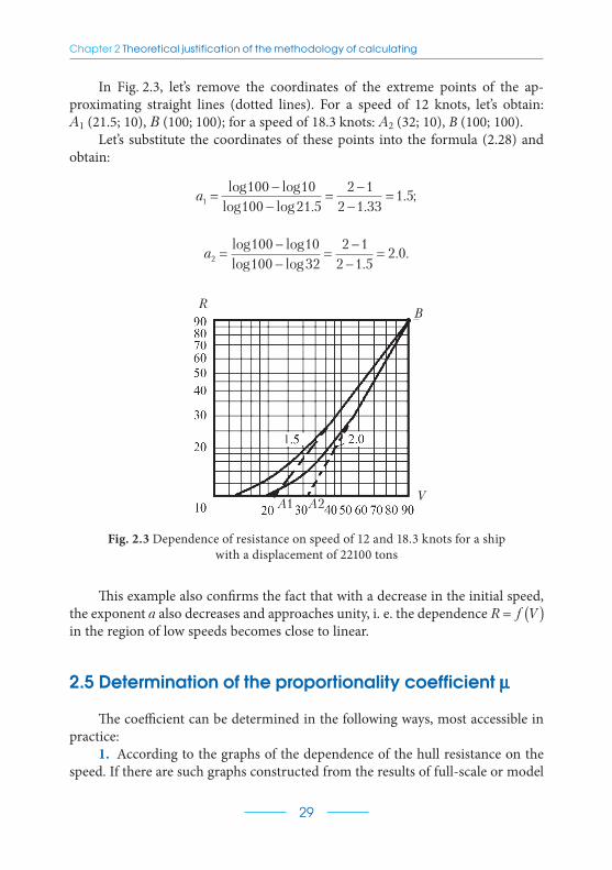
In Fig. 2.3, let’s remove the coordinates of the extreme points of the ap-proximating straight lines (dotted lines). For a speed of 12 knots, let’s obtain: A1 (21.5; 10), B (100; 100); for a speed of 18.3 knots: А2 (32; 10), В (100; 100).
Let’s substitute the coordinates of these points into the formula (2.28) and obtain:
a1
100 10
100 21 5
2 1
2 1 331 5=
−−
=−
−=
log log
log log . .. ;
a2
100 10
100 32
2 1
2 1 52 0=
−−
=−
−=
log log
log log .. .
RB
VA1 A2
Fig. 2.3 Dependence of resistance on speed of 12 and 18.3 knots for a ship with a displacement of 22100 tons
This example also confirms the fact that with a decrease in the initial speed, the exponent a also decreases and approaches unity, i. e. the dependence R f V= ( ) in the region of low speeds becomes close to linear.
2.5 Determination of the proportionality coefficient m
The coefficient can be determined in the following ways, most accessible in practice:
1. According to the graphs of the dependence of the hull resistance on the speed. If there are such graphs constructed from the results of full-scale or model
Theory and methods for calculating the inertial-braking characteristics of a ship
30
tests, then the problem is solved relatively simply. Several corresponding values of resistance and speed are removed from the graph as a percentage of their initial values and the exponent a is calculated in the manner described in subsection 2.4. Then the coefficient can be determined by the formula:
m =R
V a. (2.32)
2. According to the general formula of resistance. In accordance with the similarity theory [1], the water resistance to the ship movement is calculated by the general formula:
R V= ξρΩ2
2, from where m ξρ
=Ω2
, (2.33)
where ξ = − +0 0085 0 051 0 1246 2. . .Fr Fr – total drag coefficient obtained by ap-proximating the impedance curve of ships [2]; Fr V gL= – Froude number; g = 9 81. m/s2; L – ship length between perpendiculars, m; Ω = +(D B2 3 4 854 0. . + ( ))D B T854 0 492. . – area of wetted surface, m2; D – ship displacement, t; B/T – ratio of the width to the average draft of the ship.
The calculation of the wetted surface is carried out within the expected dis-placement of the ship. Based on the results of the calculation, a graphical depen-dence Ω = ( )f T is built, according to which, using the load scale, the value of the wetted surface is determined for any displacement.
3. By the effective power of the main engine. It is known [3] that hull resis-tance, ship speed, towing power and main engine power (in h. p.) of a ship are related to each other by the following relationships:
EPSRV
=75
; EPS Np e= ⋅ ⋅η η .
Equating the right-hand sides of these equations:
η ηm
⋅ ⋅ =s eNV 3
75, from where m
η η=
⋅ ⋅ ⋅753
s eN
V, (2.34)
where η – propulsion coefficient for a laden ship is 0.70; for a ship in ballast is 0.80; ηs – shaft line coefficient is 0.97 if the engine room is located in the middle of the ship and 0.98 if the engine room is located in the stern of the ship; Nе – effective power of the main engine, h. p.; EPS – towing power.

Chapter 2 Theoretical justification of the methodology of calculating
31
4. According to empirical formulas. The work [4] presents numerous results of full-scale and model tests of laden ships.
After processing and approximating these results, a simple empirical formula was obtained [5]:
RD
LVlad= 58 2. , form where m = 58
D
Llad . , (2.35)
where Dlad . – laden ship’s displacement, t; L – length of the ship between perpen-diculars, m.
With a Froude number:
FrV
gL= < 0 25. ,
which is usually the case for most transport ships, formula (2.35) gives satisfactory results for a laden ship.
To recalculate the coefficient m for a smaller displacement, it is possible to use the formula:
m m=
lad
lad
D
D.
.
.
.
1 167
(2.36)
2.6 Determination of the added mass coefficient k
The added mass effect occurs when a rigid hull translates in a liquid. During the acceleration and braking of the ship, the value of the added mass of water turns out to be somewhat greater than during steady motion.This is due to the fact that at unsteady motion the hull resistance becomes somewhat higher than at steady-state [6], i. e.
R R Ru= + D ,
where Ru – resistance at unsteady motion with an instantaneous value of speed, calculated as at steady motion of the ship; DR – additional resistance caused by the influence of the acceleration force.
If the value of the additional resistance is combined with the inertial force, then the coefficient of the added mass will be equal to:

Theory and methods for calculating the inertial-braking characteristics of a ship
32
kR
dV
dtm
m
m=
+=
λ11 D D:, (2.37)
where Dm – value of the added mass of water, determined by the formula [7]:
Dm T B= ⋅ ⋅1 5
42.
,πρ
(2.38)
where Т – average draft of the ship, m; В – ship width, m; π = 3 14. ...
Then the mass of the ship, taking into account the coefficient of the added mass of water, will be equal to:
m m k m+ = +( )D 1 . (2.39)
In the domestic literature [8, 9] it is accepted to consider the coefficient of the added mass k to be a constant value equal to 0.1, i. e. 10 % of the ship’s mass displacement, which is approximately suitable for medium-tonnage ships. In prac-tice, for large-capacity tankers and bulk carriers, the coefficient of added weight can be equal to 0.05 or less, and for medium-tonnage ships – 0.12 or more. Such errors can significantly distort the calculated characteristics of acceleration and braking of ships.
2.7 An example of calculating the length and time of stopping distance of a ship with active braking
Let’s take the data for the ship from article [5]. Displacement of the ship: 22100 t; (1+k).=.1.1; V0.=.9.15 m/s; Vrev..=.6.5 m/s; R0.=.688.000 H; P1.=.590700 H.
Using formulas (2.24)–(2.26), let’s determine the value of the middle thrust of the propeller:
P R R PV V
avrev
1 0 0 10
2
688000 68800 5907009 15 6 5
2
= − −( ) +=
= − −( ) += −
.
. .773372.
P Pav2 1 590700= = .
P P Pav av av= + = − =2 1
590700 73372 517328.

Chapter 2 Theoretical justification of the methodology of calculating
33
Using the formula (2.18), let’s determine the stopping distance length:
Sk mV
R
R
Pav
=+( )
+
=
=⋅ ⋅
⋅
1
21
1 1 22100000 9 15
2 688000
02
0
0
2
ln
. .lnn .1
688000
5173281242+
= m
Using the formula (2.19), let’s determine the stopping distance time:
tk mV
R
R
P
R
Pav av
=+( )
=
=⋅ ⋅
1
1 1 22100000 9 15
688000
688000
0
0
0 0arctg
. .
5517328
688000
517328318 5 3arctg s= = . min.
During acceptance tests, the following full-scale results were obtained: S f = 1215 m and t f = 4 9. min. The ratios of the calculated and full-scale values are within the experimental accuracy.
2.8 Determination of the length and time of stopping distance during passive braking
Passive braking is the slow motion of the ship after the fuel (steam) is closed to the main engine. Up to this point, the movement of the ship was steady and occurred under the action of the thrust of the propellers, which was balanced by the resistance force. From the moment the «stop» command is given until the fuel (steam) supply is stopped, the ship’s speed can be considered constant and equal to the speed of steady motion, because this period lasts only 5–10 s. The distance traveled by the ship during this period is defined as the product of time and speed of steady motion.
Then slow motion begins with the main engine dumped load. There is a rapid drop in the propeller rotational speed to the «free rotation» mode, when the pro-peller, under the action of the incident flow, operates as a hydraulic turbine. Due to the kinetic energy of the rotating masses of the engine, it still creates a certain posi-tive thrust, which gradually drops to zero. The passive braking process is described by the following equation, in which the propeller thrust force, Р1.=.0:
1 02+( ) + =k mdV
dtVm . (2.40)
Theory and methods for calculating the inertial-braking characteristics of a ship
34
The time and distance of passive braking are calculated from the initial speed, V0, and to the final speed, Vk, which is assumed to be 0.2V0, or to the speed of loss of control, whichever comes first. The solution to equation (2.40) has the following form:
tk m
V
V
Vk
=+( )
−
1
10
0
m, S
k m V
Vk
=+( )
1
0
mln . (2.41)
The propellers in the locked state can create a braking force of more than 50 % of the hull resistance force [9, 10].
The value of the resistance of the locked propeller to the movement of the ship can be calculated using the formula from the reference book [2], after bring-ing it to the SI dimensions:
RD
H
D
Vp
p
p
=⋅ ⋅ ⋅ −( )
+
477 7 1
1 0 52
2 2
2
2.
.
,Θ ψ
(2.42)
in which
m p
p
p
D
H
D
=⋅ ⋅ ⋅ −( )
+
477 7 1
1 0 52
2 2
2
.
.
.Θ Ψ
(2.43)
For freely rotating propellers, according to A. Kalmakov [2], the coefficient can be determined from the expression:
m p pD= ⋅ ⋅ −( )125 12 Θ Ψ , (2.44)
where Dp – propeller diameter, m; Θ – disc ratio of the propeller; Ψ – associated flow coefficient; H Dp – propeller pitch ratio; V – ship speed, m/s.
The total resistance of the hull and propeller will be equal to:
R V Vap= +m m 2 at a = 2, R Vp= +( )m m 2. (2.45)
For approximate calculations of the resistance of a freely rotating propeller, it can be assumed that Rp.=.0.2R, m m m+ =p 1 2. at a = 2.

Chapter 2 Theoretical justification of the methodology of calculating
35
2.9 Example of calculating the length and time of stopping distance for passive braking
To the data of the ship given in the example of subsection (2.6), let’s add ad-ditional values: propeller diameter, Dp.=.6.3 m; propeller pitch ratio, H/Dp.=.1.0; propeller disc ratio, Θ.=.0.6; associated flow coefficient, Ψ.=.0.29; final speed Vk =.3 m/s.
Using the formula (2.43), let’s determine the proportionality coefficient for the locked propeller:
m =−( )
+
=⋅ ⋅ ⋅ −( )477 7 1
1 0 52
477 7 6 3 0 6 1 0 292 2
2
2 2.
.
. . . .D
H
D
p
p
Θ Ψ
11 0 52 14651
2+ ⋅=
..
Using the formula (2.44), let’s determine the coefficient for a freely rotating propeller:
m p pD= ⋅ ⋅ −( ) = ⋅ ⋅ ⋅ =125 1 125 6 3 0 6 0 71 21132 2Θ Ψ . . . .
Using formulas (2.41), let’s determine the length and time of passive brak-ing of the ship for a locked and freely rotating propeller from the initial speed V0.=.9.15 m/s to the final speed equal to Vk.=.3.0 m/s.
For a locked propeller:
tk m
V
V
Vp k
=+( )+
−
1
10
0
( )m m.=.
1 0 1 22100000
4651 8215 9 15
9 15
31 423 7
+( )+ ⋅
−
= =.
( ) .
.min.s
Sk m V
Vp k
=+( )
+
1
0
m mln .=.
1 0 1 22100000
4651 8215
9 15
32107 11 4
+( )+
= =.
ln.
. .m cbl
For a freely rotating propeller:
tk m
V
V
Vp k
=+( )+
−
1
10
0
( )m m.=.
1 0 1 22100000
2113 8215 9 15
9 15
31 527 8 8
+( )+
−
= =.
( ) .
.. min.s
Sk m V
Vp k
=+( )
+
1
0
m mln .=.
1 0 1 22100000
2113 8215
9 15
32624 14 2
+( )+
= =.
( )ln
.. .m cbl

Theory and methods for calculating the inertial-braking characteristics of a ship
36
From a comparison of the results obtained, it can be seen that for a freely ro-tating propeller, the stopping distance of the ship is 2.8 cbl longer, and the braking time is 1.8 minutes longer.
In this case, when the resistance to motion is proportional to the square of the ship’s speed, the path length and braking time approach their values asymptotically.
Thus, as a result of the research done, calculation formulas were obtained to determine the characteristics of active and passive braking of the ship. Methods for determining the exponent and proportionality coefficient in the formula of resis-tance to the movement of the ship have been developed average value of the propel-ler thrust during reverse; resistance of a locked and freely rotating propeller during passive braking; values of the coefficient of the added mass of water during acce-lerated and decelerated movement of the ship. Examples of calculation of the length time of stopping distance of the ship with active and passive braking are given.
References
1. Katsman, F. M., Dorogostaiskii, D. V. (1979). Teoriia sudna i dvizhiteli. Lenin grad: Sudostroenie, 280.
2. Voitkunskii, Ia. I., Pershits, R. Ia., Titov, I. A. (1960). Spravochnik po teorii korablia. Leningrad: Sudpromgiz, 688.
3. Lap, A. J. W. (1954). Diagrams for determining the resistance of single-screw ships. International Shipbuilding Progress, 1 (4), 179–193. doi: http:// doi.org/10.3233/isp-1954-1403
4. Norrbin, N. H. (1971). Theory and observations on the of a mathematical model for ship manoeuvring in deep and confined waters. Trans. Swedish State Shipbuilding Experimental tank, Goteborg, 68 (19), 117.
5. Iarkin, P. I., Kalinichenko, Y. V. (2003). Opredelenie kharakteristik aktivnogo tormozheniia sudna. Alternativnii podkhod. Sudovozhdenie, 6, 159–165.
6. Hewins, E. P., Chase, H. J., Ruiz, A. L. (1950). The Backing power of geared – turbine – driven vessels. SNAME Transactions, 58, 261–301.
7. Snopkova, V. I. (Ed.) (1991). Upravlenie sudnom. Moscow: Transport, 359.8. Schetinina, A. I. (Ed.) (1983). Upravlenie sudnom i ego tekhnicheskaia eks-
pluatatsiia. Moscow: Transport, 655.9. Sainsbury, J. C. (1963). Stopping the ship. Ship and Boat Builder, 34–37.
10. Tani, H. (1968). The Reverse Stopping Ability of Supertankers. Journal of Navigation, 21 (2), 119–154. doi: http://doi.org/10.1017/s0373463300030290
37
Chapter 3 DETERMINATION OF THE CHARACTERISTICS OF THE ACTIVE SHIP BRAKING. ALTERNATIVE APPROACH
This chapter describes an alternative approach for determining the inertia-brak-ing characteristics of a ship. The method under consideration compares favorably with those widely used in that it is convenient for use directly on the navigating bridge when maneuvering a ship, since it does not require experimental data – for calculations, it is sufficient to have general characteristics of a ship at any dis-placement. Also, this approach makes it possible to exclude the traditional stages of braking in the calculations (signal passage, passive braking and active braking) and to carry out the calculation continuously from the moment the signal is sent to the engine room to the specified speed or until the ship stops completely.Keywords: alternative approach, calculation method, ship maneuvering, ship hull resistance, braking length.
Captains and their assistants are well aware that proper consideration of the inertial and braking characteristics of the ship when maneuvering in cramped conditions and in conditions of limited visibility is a guarantee of trouble- free sailing.
The graphs of inertial-braking characteristics in the form of rectangular co lumns, recommended by IMO for practical use, do not fully reflect the charac-teristics of the accelerated and decelerated movement of the ship. The linear con-struction of these graphs makes it difficult to interpolate the results depending on the value of the ship’s initial speed. When maneuvering a ship at night, it is gene-rally impossible to use them in the darkened wheelhouse of the navigating bridge.
In the scientific and educational literature, it is proposed to separately calcu-late three stages of active reversal: the time of command passage from the bridge to the engine room; passive braking time and active braking time. Such stages significantly complicate the calculation and formalization of the process; there-fore, such a calculation is not very suitable for practical purposes.
Theory and methods for calculating the inertial-braking characteristics of a ship
38
The method described below for the continuous calculation of inertial-braking characteristics, without dividing the process into the mentioned stages, was develo-ped in order to simplify the acquisition of data so important for the navigator.
3.1 Derivation of calculation formulas
If the ship in the process of braking does not deviate from the initial course (the length of the coast is equal to the length of the braking length), then the law of its motion is described by the differential equation:
( ) ,1+ = −åk mdV
dtF (3.1)
in which the sum of the braking forces Få consists of the hull resistance R and the propeller thrust to astern P, in Newtons; k – coefficient of added mass, V – ship speed, m/s, m – ship mass, kg.
The entire braking process is divided by speed into several elementary sec-tions, n n, + 1 and assumes that in each section the work of the resistance and thrust forces of the propeller is equal to the work of their average values P Rav av, . Then rewrite the right-hand side of equation (3.1) as follows:
11 1
+ = − +( ) ( )+ +k m
dV
dtR Pav avn n n n, ,
. (3.2)
In the theory of the ship, the resistance of the hull to the movement of the ship is usually approximated by a power dependence of the form:
R V a= m ,
where m – proportionality coefficient; a – exponent.To determine the average resistance at each section of speed, let’s apply the
theorem on the mean of integral calculus, according to which:
RV V
V dVV V
a Vav
n n
a na
na
nV
V
n
=−
=−( )
+( )( )+
+++
++
∫1
11
111
11
mm
, (3.3)
where Vn –initial speed before braking; Vn+1 – speed at the end of an elementary braking section.

Chapter 3 Determination of the characteristics of the active ship braking. Alternative approach
39
For the most common case, when a = 2 :
R V V V Vav n n n n= + ⋅ ++ +
m3
21 1
2( ). (3.4)
To determine the value of the aspect ratio, it is possible to use one of the methods described in chapter 2. Since the ship mass practically does not change during braking, equation (3.2) can be represented as follows:
d k mV
dtR Pav avn n n n
[( ) ]( ).
, ,
11 1
+ = − ++ +
Let’s multiply both sides of this equality by dt and take integrals from them. In this case, on the left, where the integration is in speed, the limits of the integral will be Vn and Vn+1, and on the right, where the integration is in time, the limits of the integrals will be 0 and t. As a result, let’s find that the change in the momentum of the ship in a given braking section is equal to the sum of the impulses of the forces acting on it, i. e.
( ) ( ) ., ,
1 1 1 1 1+ − + = ⋅ + ⋅+ + +
k mV k mV R t P tn n av avn n n n (3.5)
Solving equation (3.5) for t, let’s obtain:
tk m
R PV V
av av
n n
n n n n
= ++
−+ +
+
( )[ ],
, ,
1
1 1
1 (3.6)
where t – braking time in seconds. For Vn+ =1 0 :
tk mV
R Pn
av avn n n n
= ++
+ +
( )
, ,
.1
1 1
(3.7)
To find the stopping distance length, let’s represent the acceleration in equa-tion (3.2) as:
dV
dt
dV
dS
dS
dtV
dV
dS
dV
dS= = =
1
2
2
.
Then:
( )
( )., ,
1
2
2
1 1
+ = − ++ +
k mdV
dSR Pav avn n n n
(3.8)
Theory and methods for calculating the inertial-braking characteristics of a ship
40
Let’s multiply both sides of equality (3.8) by dS and introduce (1+k)m under the differential sign. Let’s obtain the expression of the theorem on the change in kinetic energy in differential form:
d dSk mV
R Pav avn n n n
( ), ,
,1 2
2 1 1
+
= − +( )+ + (3.9)
whence the stopping distance length at each section of the speed during braking is equal to:
Sk m
R PV V
av av
n n
n n n n
= ++
−+ +
+ ( )
( ),
, ,
1
21 1
21
2 (3.10)
where S – stopping distance length in meters. For Vn+ =1 0, formula (3.10) is sim-plified:
Sk mV
R Pn
av avn n n n
= ++
+ +
( )
( ), ,
.1
2
2
1 1
(3.11)
The calculation by formulas (3.6), (3.7) and (3.10), (3.11) will be the more accurate, the smaller the difference in speeds.
Let’s make one more assumption that the force of the propeller thrust is a linear function of the speed from the beginning of braking to the speed of the beginning of the reverse, Vrev., after which it becomes constant and equal to the value in the mooring mode (Fig. 1.1). At a steady ahead speed, the hull resistance will be equal to the force of the propeller thrust corrected by the co-flow coeffi-cient, i. e.:
R P0 01= −( ) ,Ψ (3.12)
where is Ψ – associated flow coefficient.With this in mind, let’s obtain expressions for determining the middle thrust
of the propeller at the given speed sections:
P R R PV
Vavav
rev
= − − ′0 0 1( ).
, where VV V
avn n=
+ +1
2. (3.13)
When V Vav rev= ., then P Pav = ′1, i. e. propeller thrust to astern in mooring mode.The thrust force of the propeller to astern in the mooring mode is determi-
ned by the formula known from the ship theory:

Chapter 3 Determination of the characteristics of the active ship braking. Alternative approach
41
P K n Dp1 1 12 4′ = ′ρ , (3.14)
where ρ = 1020 kg m3 – mass density of sea water; ′K1 – ratio of the propel-ler thrust to astern in mooring mode; n1 – rotational speed of the propeller to astern, rev/s; Dp – propeller diameter, m.
In the absence of information about the ratio of the propeller thrust to astern, its value can be determined by the formula [1]:
′ = −KH
Dp
1 0 4 0 07. . . (3.15)
Example 3.1 «Uelen» motor ship Dlad ..=.22100 t, (1+k).=.1.1, V0.=.9.15 m/s, Vrev..=.6.5 m/s, R0.=.688.000 N, P1.=.590 700 N, m.=.8215, a = 2.
The reverse is made from full ahead to «full astern».Suction coefficient during acceleration to astern τ.=.0.40 [2].The results of calculating the braking characteristics are presented in Table 3.1.
Ta b l e 3 . 1
Calculation of braking characteristics of the «Uelen» motor ship
vn, m/s vn+1, m/s vav, m/s Pav, N Rav, N S, m t, min åS åt
9.15 8.0 8.57 559638 604959 205.8 0.4 205.8 0.4
8.0 7.0 7.5 575730 462778 175.6 0.4 381.4 0.8
7.0 6.0 6.5 590700 347768 168.4 0.4 549.8 1.2
6.5 5.0 – 590700 273148 242.7 0.7 792.5 1.9
5.0 4.0 – 590700 167038 144.4 0.5 936.9 2.5
4.3 3.0 – 590700 101318 122.9 0.6 1060.0 3.0
3.0 2.0 – 590700 52028 94.6 0.7 1154.4 3.7
2.0 1.0 – 590700 19168 59.8 0.7 1214.2 4.4
1.0 0 – 590700 2738 20.5 0.6 1234.6 5.0
In full-scale tests, the following results were obtained: S f.=.1215 m and t f.=.4.9 mi-nutes. Deviations of the calculated values from the full-scale values are within the limits of accuracy determined in РШС-89 (10 % RMS).
Recall that the calculation of the length and stopping time with active braking of this ship according to the method described in Chapter 2 gave the following results:
S.=.1242 m, t.=.5.3 min.

Theory and methods for calculating the inertial-braking characteristics of a ship
42
From a comparison of the results obtained, it can be seen that both methods are, practically, equally accurate.
3.2 Influence of passing and opponent current on the braking length of the ship
The stopping distance length during braking can be significantly influenced by the fair and the adverse current [1].
The stopping distance length on the current relative to the ground Sgr will be calculated in stages and then summed up algebraically.
With a following current at the first stage, let’s calculate the stopping distance length S and the braking time t1 from the initial speed to the complete stop of the ship relative to the water, as shown in Table 3.1. At the second stage, let’s calculate the path and time of the ship’s acceleration to astern to the current speed equal to VT , or until the ship stops relative to the ground. The equation of motion in this case will take the following form:
( ) ( ) ,1 1 1+ = − ′−k mdV
dtP RT
avτ (3.16)
where τ.=.0.40 – suction coefficient.From where
tk mV
P RT
av
=+
− ′−( )
( )
1
1 1τ (3.17)
and
Sk mV
P RT
av
=+− ′−[ ]
( )
( ),
1
2 1
2
1τ (3.18)
where
RV
avT=
m 2
3. (3.19)
The calculation is carried out according to formulas (3.17)–(3.19).At the third stage, the ship, under the influence of a fair current, will travel
a path relative to the ground, equal to the product of the current speed (with a positive sign) by the total time of the two previous stages, i. e.
Chapter 3 Determination of the characteristics of the active ship braking. Alternative approach
43
S S S V t t Sk mV
P RV V tgr T
T
av
T T= − + + = −+− ′+[ ] + +2 1 2
2
1
2
1
2 1( )
( )
( ),
τ (3.20)
exclude the braking time from formula (3.20), for which express the products V tT 1 and V tT 2 through the corresponding paths. Using formulas (3.17), (3.18), let’s compose the ratio:
S
t
VT2
2 2= . (3.21)
From where V t ST 2 22= .
Let’s multiply and divide by V0 the product V tT 1. Similarly to the previous one:
V
VV t S
V
VT T
0
0 1
0
2= . (3.22)
Let’s substitute expressions (3.21), (3.22) into formula (3.20). After a simple simplification, let’s obtain a formula for determining the stopping distance length with a passing stream:
S SV
V
k mV
P Rgr
T T
av
= +
+
+− ′−[ ]1
2 1
2 10
2
1
( )
( ).
τ (3.23)
In the case of an counter current, at the first stage, let’s also calculate the stopping distance length S and the braking time t1 from the initial speed relative to the water V0 to the stop of the ship relative to the water. At the second stage, let’s calculate the stopping distance S2 and braking time t2 from the current speed VT to the stop of the ship relative to the water. The difference S S− 2 will give the stopping distance length relative to the ground. At the third stage, the ship under the influence of the adverse current will travel a path relative to the ground, equal to the current speed (with a negative sign) multiplied by the time difference between the two previous stages, i. e.
S S S V t t Sk mV
R PV t V tgr T
T
av av
T T= − − − = −+
+− +2 1 2
2
1 2
1
2( )
( )
( ). (3.24)
At low values of the current speed, the middle thrust can be approximately considered equal to the propeller thrust when rotating to astern in the mooring mode, i. e. P Pav = ′1 . Taking this into account, also replacing the products v tT 1 and v tT 2 with the corresponding stopping distances, let’s obtain the formula

Theory and methods for calculating the inertial-braking characteristics of a ship
44
for determining the stopping distance length relative to the ground in an coun-ter current:
S SV
V
k mV
R Pgr
T
o
T
av
= −
+
++ ′
12 1
2
2
1
( )
( ). (3.25)
Example 3.2 Determine the stopping distance length for the «Uelen» motor ship from full speed ahead to «full speed astern» when sailing on a following and counter current. Current speed VT .=.3 knots.=.1.54 m/s.
The rest of the data are shown in Example 3.1 and Table 3.1.When a fair current:
Sgr = +⋅
+⋅ ⋅
⋅ −1235 1
2 1 54
9 15
1 1 22100000 2 37
2 0 6 59070082
.
.
. .
.115
32 37
1733
⋅
=.
m.
When an counter current:
Sgr = −⋅
+⋅ ⋅
+ ⋅1235 1
2 1 54
9 15
1 1 22100000 2 37
2 5907008215
3
.
.
. .
22 37
868
.
= m.
Thus, on a fair current, the stopping distance length relative to the coast (ground) increased by 498 meters, and on an adverse current it decreased by 367 meters.
3.3 Determining the time and speed of the ship’s acceleration astern
In the practice of maneuvering, skippers often have to take into account the time and speed of the ship’s acceleration to astern from a stationary state to a stopping distance length equal to the length of one hull.
For example, when leaving the berth without tugs, the speed of the ship to astern at the end of the maneuver should be high enough to minimize the effect of lateral drift, and at the same time safe for timely repayment of astern inertia in a limited water area [2].
Let’s make the assumption that the maximum value of the propeller thrust during acceleration to astern occurs simultaneously with the command and re-mains constant until the end of the maneuver. In this case, the differential equa-tion of motion will take the following form:
Chapter 3 Determination of the characteristics of the active ship braking. Alternative approach
45
1 1+( ) = −( ) −k mdV
dtP Rr avτ , (3.26)
which solve according to the method described in subsection 3.1, and obtain the final formulas for determining the time, t and path length, S when accelerating the ship to astern:
tk mV
P Rr av
=+( )
−( ) −1
1 τ, (3.27)
Sk mV
P Rr av
=+( )
−( ) −
1
2 1
2
τ, (3.28)
where P K n Dr p= ′1 12 4ρ – propeller thrust to astern; R Vav = m 2 3 – average in-
tegral value of the hull resistance when the initial speed of the ship is zero;
′ = ( ) −K H Dp1 0 4 0 07. . – ratio of the propeller thrust to astern; n1 – rotational speed of the propeller to astern, rev/s; ρ = 1026 – mass density of seawater, kg/m3; Dp – propeller diameter, m; m – mass displacement of the ship, kg; k – coefficient of added mass, taken equal to 0.1 and (1+0.1).=.1.1; V – current speed of the ship to astern, m/s; H – propeller pitch, m; m = ( )58 D Lsh. , proportionality coefficient, where Dsh. – ship displacement in tons.
Let’s divide both parts of formula (3) by the length of the hull, L. By condi-tion, the ratio S L is equal to one. After simple transformations, let’s obtain the formula for determining the speed at the end of the maneuver:
VP L
k m L
r=−( )
+( ) +
2 1
12
3
τ
m. (3.29)
Let’s substitute the obtained value of speed into the formula (3.27) and obtain the time of acceleration of the ship to astern.
In the case when there is no reliable information about the suction coef-ficient to astern, then its value can be approximately taken equal to =.0.40 or (1–τ).=.0.60 during the entire acceleration time.
Example 3.3 CSL Spirit bulk carrier. D.=.87585 t. L.=.214.97 m; m.=.87585000 kg; Dp.=.7.240 m; H.=.5.185 m; H/Dp.=.0.716; n.=.66 rev/m.=.1.1 rev/s.
(1+k)m.=.1.1·87585000.=.96343500 kg.
m =⋅
=58 87585
214 9723630
..

Theory and methods for calculating the inertial-braking characteristics of a ship
46
K1.=.0.4·0.716–0.07.=.0.216. Рr..=.0.216·1026·1.12·7.244.=.738149 N.
V =⋅ ⋅ ⋅
+ ⋅= =
2 738149 214 97 0 6
963435002
323630 214 97
1 38 2 7. .
.
. .m s knotts.
t =⋅
⋅ −⋅
= =96343500 1 38
0 6 73814923630 1 38
3
310 5 22
.
..
. min.s
Conclusions. Chapter 3 describes and illustrates an alternative method for calculating the active braking of a ship. Thanks to the use of theorems on the change in the momentum and kinetic energy on an elementary interval of the ship’s slow motion speed, it was possible to exclude the traditional stages of brak-ing (signal passage, passive braking and active braking) and to carry out the cal-culation continuously from the moment the signal was sent to the engine room to a given speed or to full stopping the ship. The resulting formulas made it possible to develop a method for determining the braking length on a following and on an counter current, as well as a method for determining the speed and time of the ship’s acceleration to astern.
References
1. Iarkin, P. I., Kalinichenko, Y. V. (2003). Opredelenie kharakteristik aktivnogo tormozheniia sudna. Alternativnii podkhod. Sudovozhdenie, 6, 159–165.
2. Kalinichenko, Y. V. (2004). Opredelenie vremeni i skorosti razgona sudna na zadnii khod. Materialy mezhdunarodnoi nauchn.-tekhn. konferentsii. Chast 1. ONMA, 153–156.

47
Chapter 4 DETERMINATION OF SHIP ACCELERATION AND BRAKING CHARACTERISTICS
The chapter is devoted to the development of a methodology for analytical calculation of ship characteristics during acceleration and braking, which are often not represented at all in the data on the maneuvering properties of ships. Meanwhile, these parameters must be known for practical maneuvering to ensure safe navigation. For this reason, the question of finding suitable ma-thematical models for the movement of the ship during acceleration and brak-ing is very relevant.Keywords: analytical calculation, acceleration, braking, propeller thrust, full-scale test.
Modern ideas about the maneuvering properties of ships show that the data on the maneuvering properties available on the ship, which it is equipped with in accordance with the requirements of the International Maritime Organiza-tion (IMO) and the normative documents of Ukraine, account for only 20 % of the total number of parameters that characterize the behavior of the ship while in motion.
In addition, in the existing literature on this issue, dependences are given that do not allow obtaining the values of the time and paths traversed by ships during acceleration and braking with sufficient accuracy.
Fully maneuverable properties of the ship are characterized by the data on its inertial qualities and controllability, which are given in [1]. In addition, large-ton-nage ships have maneuverability properties that differ significantly from the charac-teristics of medium-tonnage ships, due to the presence of large inertial forces [2].
Methods for calculating the characteristics of acceleration and braking are given mainly in the educational literature [3, 4], as well as in.
In [4], when solving the differential equation, it was assumed that the pro-peller thrust during acceleration and braking remains constant, and the assigned number of revolutions occurs instantly, at the time of command. The last as-sumption can be accepted, taking into account the fact that the engine accelerates

Theory and methods for calculating the inertial-braking characteristics of a ship
48
in 3–5 seconds, and the process of changing the ship’s motion mode itself takes a considerable time.
4.1 Theoretical substantiation and derivation of calculation formulas
When the ship accelerates from the initial to the specified speed, the inertia force is equal to the difference between the thrust force of the propeller, corrected by the suction coefficient, and the force of resistance to motion, corresponding to the initial speed, i. e.
1 1+( ) = −( ) −k mdV
dtP Rτ . (4.1)
Let’s suppose that in the initial period of time the ship is moving at a slow speed at a speed equal to Vs.s. (Fig. 4.1). At point «a» the hull resistance is equal to the propeller thrust force, corrected by the suction coefficient. After the command «full speed ahead» was given, the thrust force increased to point b, resulting in an inertial force ab. Since in large-tonnage ships the development time of the full speed thrust force is an insignificant part of the time to reach the steady-state motion speed, in order to simplify the conclusions, let’s assume that the propeller thrust force reaches a given value without inertia simultaneously with the command.
a
b
P, R
R = f(U)
(1–t)Pfsa = f(U)
Pmm fs
Pmm hs
Pmm ss
Uss Uhs Ufs
U
c
d
e
Fig. 4.1 Dependence of the propeller thrust forces and resistance to movement on speed
Under the influence of the inertial force, the speed of the ship will begin to increase. When it reaches the value of the half ahead, let’s reduce the speed of the propeller and balance the thrust force with the force of resistance to move-

Chapter 4 Determination of ship acceleration and braking characteristics
49
ment (point d ). If to keep the propeller speed unchanged, then the balance of forces will come when the full speed is reached (point e). With approaching the speed of steady motion, the inertial force tends to zero and the ship’s speed will asymptotically approach its maximum value. The nature of the change in acce-leration from the speed of movement is shown in Fig. 4.2. At the initial moment of acceleration, the acceleration increases to a maximum value, then, with an in-crease in the speed of the translational movement, it decreases and becomes equal to zero with a steady movement.
Thus, with accelerated movement, the force of the propeller thrust simul-taneously with the command increases to a value 1 0 0−( ) =τ P R , and with the slow motion of the ship, the force of the propeller thrust simultaneously with the command decreases and reaches a value 1 0 0−( ) =τ P R with a decrease in speed.
Uss Uhs Ufs
U
dU/dt
Fig. 4.2 The nature of acceleration change
When the ship accelerates from a given speed (or zero speed) to a steady speed, the value of the inertia force is equal to the difference between the thrust force of the propeller, P, and the hull resistance, R, corresponding to the steady speed, i. e.
( ) ( ) ,1 1+ = − −k mdV
dtP Rτ (4.2)
where k – coefficient of the added mass of the ship; dV dt – acceleration during ship acceleration; τ – suction coefficient, taking into account the effect of the hull on the propeller operation.
To display the calculated formulas for the path and time of acceleration and braking, let’s express the thrust force using the formula:
P K n Dp= 12 4ρ , (4.3)
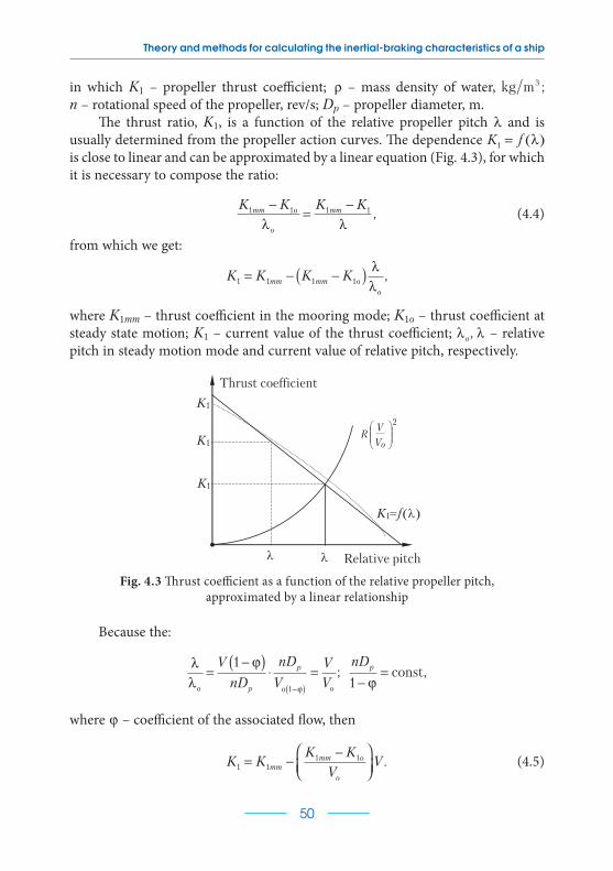
Theory and methods for calculating the inertial-braking characteristics of a ship
50
in which K1 – propeller thrust coefficient; ρ – mass density of water, kg m ;3 n – rotational speed of the propeller, rev/s; Dp – propeller diameter, m.
The thrust ratio, K1, is a function of the relative propeller pitch λ and is usually determined from the propeller action curves. The dependence K f1 = ( )λ is close to linear and can be approximated by a linear equation (Fig. 4.3), for which it is necessary to compose the ratio:
K K K Kmm o
o
mm1 1 1 1−=
−λ λ
, (4.4)
from which we get:
K K K Kmm mm o
o
1 1 1 1= − −( ) λλ
,
where K1mm – thrust coefficient in the mooring mode; K1о – thrust coefficient at steady state motion; K1 – current value of the thrust coefficient; λ λo , – relative pitch in steady motion mode and current value of relative pitch, respectively.
K1
шв
K1
K1
о
Thrust coefficient
Relative pitch
2
Vo
VR
K1 =f( λ)
λ λ
Fig. 4.3 Thrust coefficient as a function of the relative propeller pitch, approximated by a linear relationship
Because the:
λλ
ϕ
ϕo p
p
o o
V
nD
nD
V
V
V=
−( )⋅ =
−( )
1
1
; nDp
1−=
ϕconst,
where ϕ – coefficient of the associated flow, then
K KK K
VVmm
mm o
o
1 11 1= −
−
. (4.5)

Chapter 4 Determination of ship acceleration and braking characteristics
51
Substituting expressions (4.3) and (4.4) into the right-hand side of differen-tial equation (4.2), let’s obtain:
1 111 1 2 4−( ) − = −
−
⋅ −( ) −τ ρ τ mP R KK K
VV n D Vmm
mm o
o
pa , (4.6)
where R V a= m ; m – proportionality coefficient; a – exponent; Vо.=.Vst – speed of steady motion. Denote:
P K n Dmm mm p= 12 4ρ ; R P K n Do o o p= −( ) =1 1
2 4τ ρ , (4.7)
where Ro – resistance of the ship’s hull during steady motion; Рo – propeller thrust at steady motion; K1о – propeller thrust coefficient at steady motion.
After substituting (4.7) into (4.6) and expanding the brackets:
1 0 0−( ) − = −−
−τ mP R P
P R
VV Vmm
mm o
o
a . (4.8)
Let’s determine the value of the middle thrust of the propeller in a given range of acceleration speed:
P PP R
V
V Vav mm
mm o
o
= −−
+
1 2
2. (4.9)
To determine the force of the middle resistance to the movement of the ship in the same speed range, let’s again apply the theorem on the mean of the integral calculus, according to which:
RV V
a V Vav
a a
=−( )
+( ) −( )+ +m 2
11
1
2 11. (4.10)
At the most commonly used exponent, a.=.2, formula (4.10) takes the form:
R V V V Vav = + +( )m3
22
2 1 12 .
Let’s divide the entire acceleration process into several intervals in terms of speed (V1, V2, … Vn – boundaries of the intervals) and assume that in each interval the work of the resistance and thrust forces of the propeller is equal to the work of their average values. Then rewrite the right-hand side of equation (4.2) as follows:
Theory and methods for calculating the inertial-braking characteristics of a ship
52
1+( ) = −kdV
dtP Rav av , (4.11)
from which, based on the theorems about changing the momentum and kinetic energy, let’s obtain formulas for determining the time and length of the accelera-tion and braking path:
tk m
P RV V
av av
=+( )−
−[ ]12 1 ; (4.12)
Sk m
P RV V
av av
=+( )
−( ) − 1
222
12 . (4.13)
The proportionality coefficient m can be determined from the general resis-tance formula given in chapter 2:
R V= ξρΩ2
2, from where m ξρ
=2
Ω, (4.14)
where ξ = − +0 0085 0 051 0 1246 2. . .Fr Fr – impedance coefficient of ships, obtained by approximating the impedance curve; Fr V gL= – Froude number; g.=.9.81 m/s2; L – length of the ship between perpendiculars, m; Ω= + ( )( )D B T2 3 4 854 0 492/ . . – wetted surface area, m2; D – ship displacement, t; B/Т – ratio of the ship’s width to the mean draft.
The ahead propeller thrust coefficient in the mooring mode can be deter-mined either from the curves of the action of the propellers, or by the formula:
KH
Dmm
p
1 0 4 0 018= +. . . (4.15)
The added mass effect occurs when a solid moves in a liquid. During accele-ration and braking of the ship, the value of the added mass can be calculated using the formula given in chapter 2:
Dm T B=1 5
42.
,πρ
(4.16)
where T – ship draft, m; В – ship width, m; π = 3 14. ...
Then the ship mass, taking into account the coefficient of added mass, will be:
m m k m+ = +( )D 1 . (4.17)
Chapter 4 Determination of ship acceleration and braking characteristics
53
4.2 The procedure for calculating the path length and acceleration and braking time for «Vasily Porik» motor ship
Ship displacement, Ds.=.29100 t; length between perpendiculars, L.=.174 m; width, B.=.23.0 m; average draft T.=.9.5 m; propeller diameter, Dp.=.5.9 m; propeller pitch, H.=.5.04 m; propeller rotation frequency for ahead motion, nо.=.1.415 rev/m; ship speed at nо, Vо.=.6.69 m/s, full ahead speed, Vff.=.8.75 m/s.
The calculation results are presented in Table 4.1:
1. Dm =⋅ ⋅
⋅ ⋅ =1 5 3 14 1020
49 5 23 0 24930792. .
. . kg; k = =2493079
291000000 08. .
2. 1 31593080+( ) =k m kg.
3. m = 0 00351020
25719. .=.10234; Ro = ⋅ =10234 6 69 4580532. N.
4. R V V V Vav = + +( )10234
322
2 1 12 .
5. K mm1 0 45 04
5 90 018 0 359= + =.
.
.. . .
6. Pmm = ⋅ ⋅ ⋅ =0 359 1020 1 415 5 9 8901342 4. . . .N
7. P Vav av= −−
890134890134 458053
6 69..
8. tP R
V Vav av
=−
−[ ]315930802 1 ; S
P RV V
av av
=( )
−( ) − 31593080
222
12 .
Table 4.2 shows the results of field measurements of the path and accelera-tion time of the «Vasily Porik» motor ship from a stationary state to a speed of 12 knots (6.2 m/s).
According to Table 4.1 and Table 4.2, the largest discrepancies between the full-scale and calculated curves were 5 % in time and 10 % in the path length. This testifies to the accuracy of the proposed method acceptable for practice.
The calculation results are shown in Table 4.1, it is convenient to represent in the form of graphs dependences v f S= ( ) and v f t= ( ), in which the accele-ration and braking curves asymptotically approach the ship speed during steady motion (Fig. 4.4, 4.5).

Theory and methods for calculating the inertial-braking characteristics of a ship
54
Ta b l e 4 . 1
Characteristics of acceleration and braking of the «Vasily Porik» motor ship
v1, m/s v2, m/s vav, m/s Sm tc ∑Sm ∑tc ∑tmin
Acceleration
0 1 0.5 18.5 37.0 18.5 37.0 0.62
1 2 1.5 61.6 41.0 80.1 78.0 1.30
2 3 2.5 119.0 47.6 199.0 126.0 2.10
3 4 3.5 205.6 59.0 405.0 184.0 3.00
4 5 4.5 363.0 80.7 768.0 265.0 4.40
5 6 5.5 774.0 141.0 1542.0 406.0 6.70
Braking
8.7 8 8.35 508.5 61.0 508.5 61.0 1.00
8 7.5 7.75 543.0 70.0 1051.0 131.0 2.20
7.5 7 7.25 985.0 136.0 2036.0 267.0 4.40
Ta b l e 4 . 2
Acceleration from motionless state of the «Vasily Porik» motor ship
Acceleration time, min – s
Acceleration path, m
Acceleration time, min – s
Acceleration path, m
0 0 05–20 930
02–21 186 05–55 1116
03–18 372 06–26 1302
04–05 558 06–58 1488
04–45 744
V, m/s
0123456789
10
0 400 800 1200 1600 2000
Vst
Acceleration
Braking
S, m
Fig. 4.4 Dependence of speed on the path of acceleration and braking of the «Vasily Porik» motor ship
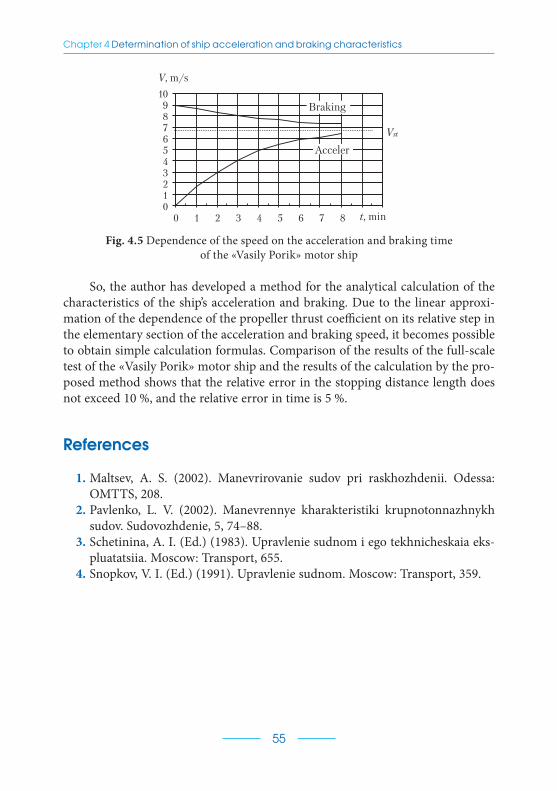
Chapter 4 Determination of ship acceleration and braking characteristics
55
V, m/s
0123456789
10
0 1 2 3 4 5 6 7 8
Vst
Acceler
Braking
t, min
Fig. 4.5 Dependence of the speed on the acceleration and braking time of the «Vasily Porik» motor ship
So, the author has developed a method for the analytical calculation of the characteristics of the ship’s acceleration and braking. Due to the linear approxi-mation of the dependence of the propeller thrust coefficient on its relative step in the elementary section of the acceleration and braking speed, it becomes possible to obtain simple calculation formulas. Comparison of the results of the full-scale test of the «Vasily Porik» motor ship and the results of the calculation by the pro-posed method shows that the relative error in the stopping distance length does not exceed 10 %, and the relative error in time is 5 %.
References
1. Maltsev, A. S. (2002). Manevrirovanie sudov pri raskhozhdenii. Odessa: OMTTS, 208.
2. Pavlenko, L. V. (2002). Manevrennye kharakteristiki krupnotonnazhnykh sudov. Sudovozhdenie, 5, 74–88.
3. Schetinina, A. I. (Ed.) (1983). Upravlenie sudnom i ego tekhnicheskaia eks-pluatatsiia. Moscow: Transport, 655.
4. Snopkov, V. I. (Ed.) (1991). Upravlenie sudnom. Moscow: Transport, 359.

56
Chapter 5 PRACTICAL APPLICATION OF INERTIAL-BRAKING CHARACTERISTICS OF A SHIP
The chapter presents a universal methodology for practical calculation of the safe speed of a ship, taking into account its inertial-braking characteristics, which sig-nificantly expands the boat master’s capabilities for efficient and safe ship control.The obtained analytical dependencies make it possible to apply the automation of the speed selection using a personal computer directly on the navigation bridge.Keywords: safe speed, ship convergence, radar station, inertial-braking charac-teristics, braking length, navigation in ice.
5.1 Calculation of safe speed and minimum permissible distance of ship convergence
The International Regulations for the Prevention of Collisions at Sea, 1972 (COLREGs-72) introduce such interrelated concepts as «safe speed» and «close proximity of ships».
When setting a safe speed, the rules recommend, among other factors, to take into account the state of visibility, the maneuverability of the ship, especially the distance required to bring the ship to a complete stop, as well as the character-istics, effectiveness and limitations of radar equipment.
COLREGs strongly recommend the use of radar equipment to detect exces-sive proximity and the presence of a collision hazard. In addition to qualitative recommendations, COLREGs-72 do not contain any quantitative assessments of the safe speed and excessive proximity of ships. Each master subjectively assigns a safe speed and determines the minimum permissible distance of approach of ships. Because of this, in almost every case of collisions between ships, the main reasons are a significant excess of the safe speed and an underestimated distance of the permissible approach of ships.
In domestic and foreign literature, a large number of publications are devo-ted to the study of errors in technical means, in determining the elements of the movement of dangerous ships and assigning the minimum permissible distance

Chapter 5 Practical application of inertial-braking characteristics of a ship
57
of convergence to them. The most complete source on this issue is the work [1, 2]. However, the publications do not contain the formulation and solution of the problem of the mutual dependence of the safe speed and the minimum permis-sible distance of approach of ships.
The aim of this research is to develop a universal method for calculating the safe speed and the minimum allowable distance, taking into account the inertial and braking characteristics of the ship when using radar information [3].
The minimum permissible distance will be determined by the radius of the danger zone of ship convergence, Rd z. ..
When using a radar station, the radius of the danger zone of ship conver-gence can be determined from the following expression [4]:
R a Sd z v. . ,= + 2 (5.1)
whence the limiting value of the safe speed should be considered the speed at which the braking length will be equal to:
S R av d z= −( )1
2. . , (5.2)
where Rd z. . – radius of the danger zone; Sv – length of the braking length of the ship at the initial speed v; a – radar parameter.
As can be seen from formulas (5.1) and (5.2), the radius of the danger zone and the value of the safe speed depend on the braking characteristics of the ship and the radar parameter, which must take into account the technical capabilities of the radar to detect the danger of the echo of another ship entering the danger zone. The parameter a is quantitatively expressed by distance, so its value can be represented as a dependence:
a V T= 0 , (5.3)
where V0 – relative speed of approach of ship; T – observation time required to detect a dangerous ship convergence with the required accuracy.
The shortest distance of ship convergence is determined by the formula:
d dV
sh =′2
0
θ, (5.4)
where dsh – shortest distance of ship convergence; d – detection range of a ship convergence; ′θ – rate of bearing change.
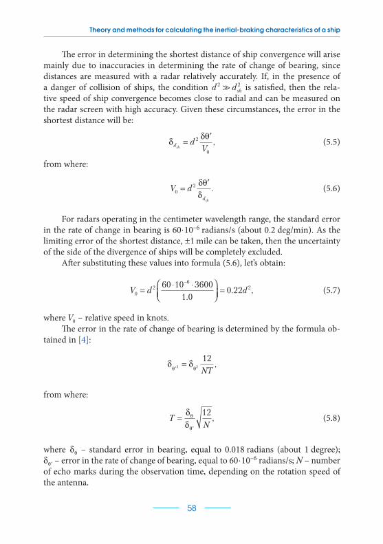
Theory and methods for calculating the inertial-braking characteristics of a ship
58
The error in determining the shortest distance of ship convergence will arise mainly due to inaccuracies in determining the rate of change of bearing, since distances are measured with a radar relatively accurately. If, in the presence of a danger of collision of ships, the condition d dsh
2 2 is satisfied, then the rela-tive speed of ship convergence becomes close to radial and can be measured on the radar screen with high accuracy. Given these circumstances, the error in the shortest distance will be:
δδθ
dshd
V=
′2
0
, (5.5)
from where:
V ddsh
02=
′δθδ
. (5.6)
For radars operating in the centimeter wavelength range, the standard error in the rate of change in bearing is 60 ⋅10–6 radians/s (about 0.2 deg/min). As the limiting error of the shortest distance, ±1 mile can be taken, then the uncertainty of the side of the divergence of ships will be completely excluded.
After substituting these values into formula (5.6), let’s obtain:
V d d02
6260 10 3600
1 00 22=
⋅ ⋅
=−
.. , (5.7)
where V0 – relative speed in knots.The error in the rate of change of bearing is determined by the formula ob-
tained in [4]:
δ δθ θ′
=2 2
12
NT,
from where:
TN
=′
δδ
θ
θ
12, (5.8)
where δθ – standard error in bearing, equal to 0.018 radians (about 1 degree); δθ′ – error in the rate of change of bearing, equal to 60 ⋅10–6 radians/s; N – number of echo marks during the observation time, depending on the rotation speed of the antenna.

Chapter 5 Practical application of inertial-braking characteristics of a ship
59
Substituting these values into the formula (5.8), let’s obtain:
TN N
=⋅
=−
0 018
60 10
12 10386
.. (5.9)
The rotation speed of the antennas of ship radars is not less than 15 rpm, therefore the value N can be obtained from the expression:
N T=1
4. (5.10)
Substituting expression (5.10) into formula (5.9), let’s find the minimum observation time for the given conditions:
T = ⋅ = =4 1038 163 0 04523 s h. . (5.11)
Let’s express the parameter in terms of the echo signal detection range:
a V T d d= ⋅ = ⋅ =02 20 22 0 045 0 01. . . . (5.12)
Taking this expression into account, formula (5.1) takes the following form:
R d Sd z v. . .= +0 01 22 (5.13)
and correspondingly,
S R dv d z= −( )1
20 01 2
. . . . (5.14)
The influence of parameter «a» on the radius of the danger zone is schema-tically shown in Fig. 5.1. Due to the presence of errors in the assessment of the collision hazard, the position of the target on the radar screen can be conven-tionally represented as a shaded area of a circle with a radius numerically equal to the parameter. Since the parameter is a function of the distance at which the collision hazard is determined, the echo area will decrease with decreasing this distance. To ensure that the echo of another ship travels from the observer ship at a distance of at least two stopping distances, the value of the parameter should be added to this distance.
Let’s consider examples of calculating the radius of the danger zone and the braking length at a given speed for a specific ship, the calculation of the braking characteristics of which is given in chapter 3.
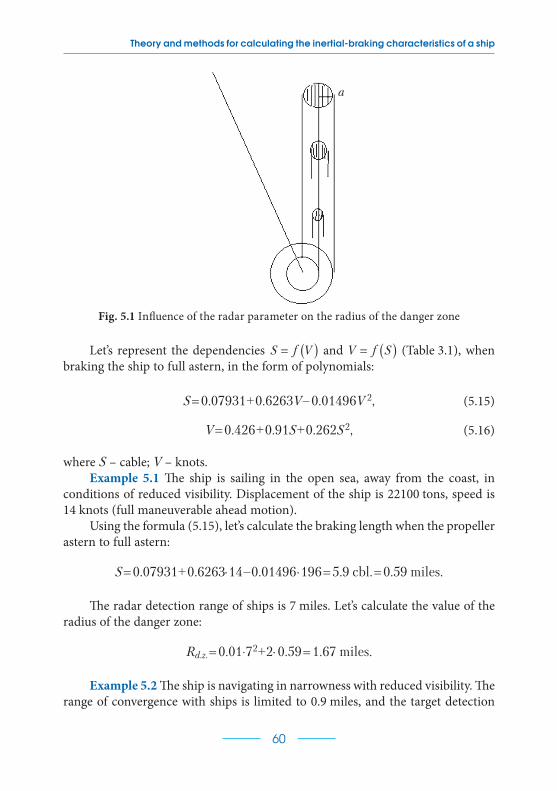
Theory and methods for calculating the inertial-braking characteristics of a ship
60
a
Fig. 5.1 Influence of the radar parameter on the radius of the danger zone
Let’s represent the dependencies S f V= ( ) and V f S= ( ) (Table 3.1), when braking the ship to full astern, in the form of polynomials:
S.=.0.07931+0.6263V–0.01496V 2, (5.15)
V.=.0.426+0.91S+0.262S2, (5.16)
where S – cable; V – knots.Example 5.1 The ship is sailing in the open sea, away from the coast, in
conditions of reduced visibility. Displacement of the ship is 22100 tons, speed is 14 knots (full maneuverable ahead motion).
Using the formula (5.15), let’s calculate the braking length when the propeller astern to full astern:
S.=.0.07931+0.6263⋅14–0.01496 ⋅196.=.5.9 cbl..=.0.59 miles.
The radar detection range of ships is 7 miles. Let’s calculate the value of the radius of the danger zone:
Rd.z..=.0.01⋅72+2⋅0.59.=.1.67 miles.
Example 5.2 The ship is navigating in narrowness with reduced visibility. The range of convergence with ships is limited to 0.9 miles, and the target detection

Chapter 5 Practical application of inertial-braking characteristics of a ship
61
range is limited to a five-mile radar scale. Based on these conditions, it is required to determine a safe speed.
Using formula (5.2), let’s find the braking length:
Sv = − ⋅( ) =1
20 9 0 01 5 0 322. . . miles.=.3.2 cbl.
At Sv.=.3.2 kbt, the safe speed will be:
V.=.0.426+0.9101⋅3.2+0.262⋅10.24.=.6.0 knots.
If the observer’s ship, for any reason, is unable to prevent excessive approach to another ship or if it hears an audible fog signal ahead of its traverse, then ac-cording to rule 19 of the COLREGs 72 it must reduce its speed to the minimum until the danger of collision has passed.
5.2 Accounting for stopping distance when ships navigate in ice behind the icebreaker
To substantiate the choice of the parameters of the movement of the con-voy of ships in the ice behind the icebreaker, let’s designate the length of the convoy (from the stern of the icebreaker to the stern of the last ship) through lk , assuming that there are n ships in the convoy (Fig. 5.2).
l d L d L d Lk n n= + + + + + +1 1 2 2 ... , (5.17)
where di – distance from the bow of the i-th ship to the stern of the ship in front (or from the stern of the icebreaker, if i.=.1):
d1 d2 dn LnL1 L2
Icebreaker
Fig. 5.2 Scheme of the caravan formation
The time during which the caravan travels a distance equal to its length lk will be equal to:

Theory and methods for calculating the inertial-braking characteristics of a ship
62
td L d L d L
Vn
n n
k
=+ + + + + +1 1 2 2 ...
, (5.18)
where Vk – caravan speed.Obviously, the sooner the caravan travels a distance equal to its length, the
less the channel pierced by the icebreaker will drag out.However, it is necessary to comply with the condition that the distance
between every two ships is not less than the stopping distance of the ship going behind, so that heap can be prevented in the event of a delay of the ship in front.
The most favorable speed of the caravan is determined by the captain of the icebreaker. At the same time, it takes into account the state of the ice, meteoro-logical conditions and the technical condition of the ships in the caravan. Masters of ships in a convoy determine the braking length of their ship and maintain an appropriate distance between ships.
For example, the captain of an icebreaker assigned the speed of the cara-van to be 6 knots. Using the formula (5.15), let’s determine the braking length of the ship:
S.=.0.07931+0.6263V–0.01496V2.=
=.0.07931+0.6263⋅6–0.01496⋅36.=.3.3 cbl.
The captain of the ship must keep at least such a distance from the icebreaker or the ship in front, in order, if necessary, to completely extinguish the inertia of the ship.
Conclusions. As a research result, an analytical relationship is obtained between the safe speed and the minimum permissible distance of approach of ships when using radar information. The developed technique makes it possible to automate the choice of a safe speed and exclude the subjective factor when it is assigned by the navigator.
The calculation of the braking length of the ship is shown when navigating in ice behind the icebreaker.
References
1. Motora, S. (1972). Maneuverability, state of the art. Proceedings of the In-ternational Jubilee Meeting on the occasion of the 40th anniversary of the Netherlands Ship Model Basin, 38.

Chapter 5 Practical application of inertial-braking characteristics of a ship
63
2. Scripture, F. R. (1966). Marine Radar Collision Avoidance System Re-quirements. Navigation, 13 (4), 295–301. doi: http://doi.org/10.1002/ j.2161-4296.1966.tb02172.x
3. Kalinichenko, G., Kalinichenko, Y. (2018). Calculation of safe speed and minimally admissible distance of closing of ships during radar information usage. Technology Transfer: fundamental principles and innovative technical solutions. Tallinn, 58–60. doi: http://doi.org/10.21303/2585-6847.2018.00758
4. Tsurban, A. I. (1977). Opredelenie manevrennykh elementov sudna. Mos-cow: Transport, 126.

64
Chapter 6 PRACTICAL CALCULATION OF INERTIAL-BRAKING CHARACTERISTICS FOR THE «ELQUI» CONTAINER CARRIER
The final chapter presents the result of applying the above-described method for determining inertial-braking characteristics using the example of the «ELQUI» container ship, on which the author worked as a captain. A practical calcula-tion, construction and implementation of working schedules of inertial-braking characteristics were carried out [1].Keywords: laden ship, ship in ballast, active braking, passive braking, braking, acceleration, braking length.
6.1 Ship data
Ship name: «ELQUI» container ship.Year of construction: 1999.Length (full): 184.1 m.Length between perpendiculars: 176.0 m.Width: 25.3 m.Laden displacement: 30843 t.Laden draft, Tav.=.9.891 m.Ballast displacement: 17655 tons.Draft, Tn.=.4.7 m; Tk.=.8.7 m; Tav.=.6.7 m.Main engine: Sulzer.Engine power: 13320 kW/17862.4 h. p.Propeller: right hand rotation.Number of blades: 5.Propeller diameter: 6.150 m.Propeller pitch: 6.101 m.

Chapter 6 Practical calculation of inertial-braking characteristics for the «ELQUI» container carrier
65
Stepping ratio: 0.9921.Disc ratio: 0.55.Steering wheel: semi-balanced.Associated flow coefficient is 0.29.
Full speed (sea): 113 rpm. 19.5 knots (laden); 19.75 knots (ballast).Full speed (maneuverable): 80 rpm. 14.2 knots (laden); 14.4 knots (ballast).Half speed: 69 rpm. 12.1 knots (laden); 12.4 knots (ballast).Slow speed: 46 rpm. 8.2 knots (laden); 8.4 knots (ballast).Dead slow speed: 36 rpm. 6.1 knots (laden); 6.4 knots (ballast).
Dead slow speed astern: 36 rpm.Slow speed astern: 46 rpm.Half speed astern: 69 rpm.Full speed astern: 80 rpm.
Programs for calculating inertial-braking characteristics are developed in the Delphi programming language. The listing of programs is presented in the author’s thesis [2].
6.2 Calculation of active braking characteristics
Initial data:
Laden ship displacement: 30 843 t.Length between perpendiculars: 176.0 m.Width: 25.3 m.Propeller diameter: 6.15 m.Propeller pitch: 6.101 m.Step ratio: 0.9921Propeller turns to astern: 80 rpm.=.1.33 rpm.Initial speed: 14.2 knots.=.7.31 m/s.Speed before reverse: 10 knots.=.5.2 m/s.End speed: 0.Number of calculated points: 10.Ship displacement in Ballast: 17654.7Average draft in ballast: 6.7 m.Initial speed in ballast: 14.4 knots.=.7.42 m/s.The calculation results are presented in Tables 6.1, 6.2 based on them graphs
V.=.f(S) and V.=.f(t), which are presented below.

Theory and methods for calculating the inertial-braking characteristics of a ship
66
Ta b l e 6 . 1Calculation results for a laden ship
Vn, knots Vn, m/s Vn+1, m/s Vav, m/s Sum S, cbl Sum t, min.14.2 7.31 6.58 6.94 0.64 0.2812.8 6.58 5.85 6.21 1.28 0.6011.3 5.85 5.12 5.48 1.90 0.959.9 5.12 4.38 4.75 2.49 1.338.5 4.38 3.65 4.02 3.02 1.747.1 3.65 2.92 3.29 3.48 2.175.7 2.92 2.19 2.56 3.86 2.624.2 2.19 1.46 1.83 4.13 3.092.8 1.46 0.73 1.09 4.30 3.581.4 0.73 0 0.36 4.36 4.06
Ta b l e 6 . 2Calculation results for a ship in ballast
Vn, knots Vn, m/s Vn+1, m/s Vav, m/s Sum S, cbl Sum t, min.14.4 7.42 6.68 7.05 0.39 0.1712.9 6.68 5.94 6.31 0.78 0.3611.5 5.94 5.19 5.56 1.16 0.5710.1 5.19 4.52 4.82 1.51 0.808.6 4.52 3.71 4.08 1.83 1.047.2 3.71 2.97 3.34 2.11 1.295.8 2.97 2.23 2.60 2.33 1.564.3 2.23 1.48 1.85 2.49 1.832.9 1.48 0.74 1.11 2.59 2.101.4 0.74 0 0.37 2.62 2.38
Dependence S(v)
V, knots
S, c
able
Fig. 6.1 Dependence of the active braking distance on the speed for a laden ship
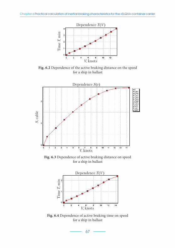
Chapter 6 Practical calculation of inertial-braking characteristics for the «ELQUI» container carrier
67
V, knots
Dependence T(V)
Tim
e T
, min
Fig. 6.2 Dependence of the active braking distance on the speed for a ship in ballast
Dependence S(v)
V, knots
S, c
able
Fig. 6.3 Dependence of active braking distance on speed for a ship in ballast
V, knots
Dependence T(V)
Tim
e T
, min
Fig. 6.4 Dependence of active braking time on speed for a ship in ballast

Theory and methods for calculating the inertial-braking characteristics of a ship
68
6.3 Calculation of the characteristics of the ship’s acceleration from a stationary state to the speed of full maneuvering speed
Ta b l e 6 . 3
Calculation results for a laden ship
Vn, knots V1, m/s V2, m/s Vav, m/s Sum S, cbl Sum t, min.
0 0 1.3 0.65 0.15 0.71
2.5 1.3 2.6 1.95 0.67 1.53
5.0 2.6 3.9 3.25 1.72 2.53
7.6 3.9 5.2 4.5 3.74 3.90
10.0 5.2 6.5 5.85 8.34 6.33
Fig. 6.5 Dependence of the acceleration path on the speed for the laden ship
Dependence V(S)
S, cable
V, k
no
ts
V, k
no
ts
Dependence V(T)
Time T, min
Fig. 6.6 Dependence of acceleration time on speed for a laden ship
Note. Since the dependences of the path length and the acceleration time of the ship asymptotically approach the value of the steady ahead speed, the calcula-tion should be carried out, up to approximately 0.9Vst.

Chapter 6 Practical calculation of inertial-braking characteristics for the «ELQUI» container carrier
69
6.4 Calculation of the characteristics of the laden ship braking from full maneuverability to the dead slow ahead speed
Ta b l e 6 . 4
Calculation results for a laden ship
Vknots V1, m/s V2, m/s Vav, m/s Sum S, cbl Sum t, min.
14.2 7.31 6.92 7.12 0.67 0.29
13.4 6.93 6.55 6.74 1.39 0.62
12.7 6.55 6.17 6.36 2.18 1.00
11.9 6.17 5.79 5.98 3.06 1.46
11.2 5.79 5.40 5.60 4.04 2.00
10.5 5.40 5.02 5.21 5.18 2.66
9.7 5.02 4.64 4.83 6.50 3.52
9.0 4.64 4.26 4.45 8.15 4.66
8.3 4.26 3.88 4.07 10.38 6.35
7.5 3.88 3.5 3.69 13.96 9.34
V, k
no
ts
Dependence V(S)
S, cable
Fig. 6.7 Dependence of the braking distance on speed
V, k
no
ts
Time T, min
Dependence V(T)
Fig. 6.8 Dependences of braking time on speed for a laden ship
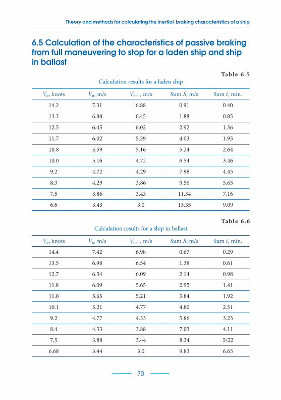
Theory and methods for calculating the inertial-braking characteristics of a ship
70
6.5 Calculation of the characteristics of passive braking from full maneuvering to stop for a laden ship and ship in ballast
Ta b l e 6 . 5
Calculation results for a laden ship
Vn, knots Vn, m/s Vn+1, m/s Sum S, m/s Sum t, min.
14.2 7.31 6.88 0.91 0.40
13.3 6.88 6.45 1.88 0.85
12.5 6.45 6.02 2.92 1.36
11.7 6.02 5.59 4.03 1.95
10.8 5.59 5.16 5.24 2.64
10.0 5.16 4.72 6.54 3.46
9.2 4.72 4.29 7.98 4.45
8.3 4.29 3.86 9.56 5.65
7.5 3.86 3.43 11.34 7.16
6.6 3.43 3.0 13.35 9.09
Ta b l e 6 . 6
Calculation results for a ship in ballast
Vn, knots Vn, m/s Vn+1, m/s Sum S, m/s Sum t, min.
14.4 7.42 6.98 0.67 0.29
13.5 6.98 6.54 1.38 0.61
12.7 6.54 6.09 2.14 0.98
11.8 6.09 5.65 2.95 1.41
11.0 5.65 5.21 3.84 1.92
10.1 5.21 4.77 4.80 2.51
9.2 4.77 4.33 5.86 3.23
8.4 4.33 3.88 7.03 4.11
7.5 3.88 3.44 8.34 5/22
6.68 3.44 3.0 9.83 6.65

Chapter 6 Practical calculation of inertial-braking characteristics for the «ELQUI» container carrier
71
V, knots
Dependence S(v)
S, c
able
Fig. 6.9 Dependence of the stopping distance on the speed of passive braking for a laden ship
V, knots
Dependence T(V)
Tim
e T
, min
Fig. 6.10 Dependence of time on the speed of passive braking for a laden ship
V, knots
Dependence S(v)
S, c
able
Fig. 6.11 Dependence of the path length on the passive braking speed for a ship in ballast

Theory and methods for calculating the inertial-braking characteristics of a ship
72
Dependence T(V)
Tim
e T
, min
V, knots
Fig. 6.12 Dependence of time of passive braking speed for a ship in ballast
6.6 Calculation of the speed and time of acceleration of a laden ship at full speed astern from a stationary state to a stopping distance length equal to the length of the ship’s hull
Initial data:
L.=.176 m; Ds.=.30843 t; Dst.=.6.15 m; Нst.=.6.101 m; Нst/Dst.=.0.9921;
ns.a.=.1.33 rev/s; suction coefficient.=.0.40;
(1+k)m.=.1.1.=.33927300 kg;
m =⋅
=58 30843
17610164; K1.=.0.4⋅0.9921–0.07.=.0.327;
Рr..=.0.327⋅1026⋅1.332⋅6.154.=.848 983 N;
V =⋅ ⋅ ⋅
+ ⋅= =
2 848983 176 0 6
339273002
310164 176
2 26 4 4.
. .m s knots;
t =⋅
⋅ −⋅
= =33927300 2 26
0 6 84898310164 2 26
3
156 2 62
.
..
. min.s
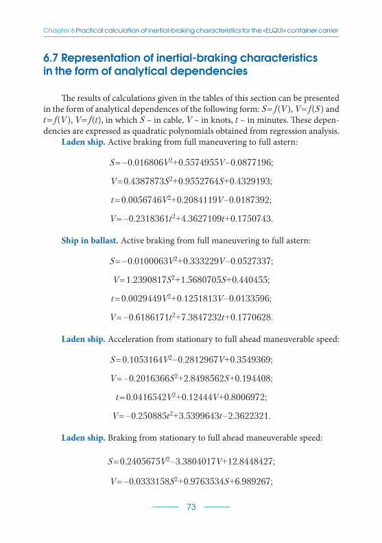
Chapter 6 Practical calculation of inertial-braking characteristics for the «ELQUI» container carrier
73
6.7 Representation of inertial-braking characteristics in the form of analytical dependencies
The results of calculations given in the tables of this section can be presented in the form of analytical dependences of the following form: S.=.f(V ), V.=.f(S) and t.=.f(V ), V.=.f(t), in which S – in cable, V – in knots, t – in minutes. These depen-dencies are expressed as quadratic polynomials obtained from regression analysis.
Laden ship. Active braking from full maneuvering to full astern:
S.=.–0.016806V2+0.5574955V–0.0877196;
V.=.0.4387873S2+0.9552764S+0.4329193;
t.=.0.0056746V2+0.2084119V–0.0187392;
V.=.–0.2318361t2+4.3627109t+0.1750743.
Ship in ballast. Active braking from full maneuvering to full astern:
S.=.–0.0100063V2+0.333229V–0.0527337;
V.=.1.2390817S2+1.5680705S+0.440455;
t.=.0.0029449V2+0.1251813V–0.0133596;
V.=.–0.6186171t2+7.3847232t+0.1770628.
Laden ship. Acceleration from stationary to full ahead maneuverable speed:
S.=.0.1053164V2–0.2812967V+0.3549369;
V.=.–0.2016366S2+2.8498562S+0.194408;
t.=.0.0416542V2+0.12444V+0.8006972;
V.=.–0.250885t2+3.5399643t–2.3622321.
Laden ship. Braking from stationary to full ahead maneuverable speed:
S.=.0.2405675V2–3.3804017V+12.8448427;
V.=.–0.0333158S2+0.9763534S+6.989267;

Theory and methods for calculating the inertial-braking characteristics of a ship
74
t.=.0.2215836V2–3.6018903V+15.2008528;
V.=.–0.0963039t2+1.611298t+7.398181.
Laden ship. Passive braking from full ahead speed to stop:
S.=.0.0898451V2–0.2458343V–1.3230324;
V.=.–0.0203645S2+0.8919579S+5.8667285;
t.=.0.1208864V2–1.4147753V+4.6278166;
V.=.–0.0803835t2+1.5927627t+6.2120366.
Ship in ballast. Passive braking from full ahead speed to stop:
S.=.0.0635215V2–0.1708933V–0.9439139;
V.=.–0.0386617S2+1.2426293S+5.8803897;
t.=.0.0856813V2–1.0192293V+3.4054004;
V.=.–0.1556919t2+2.2406684t+6.2405428.
It is convenient to use the obtained analytical dependences directly on the navigating bridge, having previously entered the necessary polynomial coeffi-cients into the computer or calculator memory.
References
1. Kalinichenko, Y. (2017). Calculation of ship’s active braking characteristics. Technology Transfer: fundamental principles and innovative technical solu-tions. Tallinn, 42–44. doi: http://doi.org/10.21303/2585-6847.2017.00474
2. Kalinichenko, Y. V. (2017). Vdoskonalennia alhorytmiv informatsiionoho za-bezpechennia manevruvannia suden. Odessa, 252. Available at: http://onma.edu.ua/wp-content/uploads/2016/09/disser_kalin.pdf
75
GENERAL CONCLUSIONS
The performed theoretical and experimental studies makes it possible to develop and test in practice methods for calculating the inertial characteristics of a ship during its acceleration and braking, when the propeller is reversed from ahead to astern and during passive braking, taking into account the impact on the ship of the passing and opponent currents. The developed methods provide the calculation of inertial characteristics with an accuracy comparable to the results of full-scale tests, which makes it possible to abandon traditional expensive full-scale tests and at the same time significantly increase the amount of useful information on the navigating bridge, which increases the level of safety when navigating a ship in confined navigation conditions.
The research results can be qualified as a theoretical generalization and practical solution of a major scientific problem, which is important for ensuring the safety of ship navigation.
For the first time, a methodology for calculating the path and time of acceleration and braking of a ship, suitable for direct use in practice, is created and formalized. The technique is based on the application of theorems about the change in momentum and kinetic energy. The work of the forces of resistance to movement and the propeller thrust is equated, respectively, to the work of their mean integral and arithmetic mean values. The change in the propeller thrust coefficient during acceleration and braking of the ship as a function of the relative step is approximated by a linear relationship. Comparison of the calculated characteristics with the experimental ones is made for the «Vasily Porik» motor ship. The discrepancy between the ex-perimental and calculated data is: along the acceleration path 2 %, in the acceleration time 5 %.
An alternative method is created for calculating and constructing working graphs of the path length and braking time of the ship when the propeller is reversed from ahead to astern. For the first time in the design formulas, the drag force to the movement of the ship is presented proportional to the speed value in any positive power, and the propeller stop force is approximated by two linear equations. The value of the exponent in the formula for resistance to motion is proposed to be determined as the slope of a straight line drawn tangent to the resistance curve plotted on a logarithmic paper. A verification calculation of inertial-braking characteristics for a full-scale ship is made. The calculation results are com-pared with the experimental data. The relative error of the calculation method is five percent.
A method is developed for calculating the speed and time of a ship’s acceleration to astern from a stationary state to a stopping length equal to the length of one hull.
Software is created in the Delphi programming language.According to the developed methods, practical calculation, construction and im-
plementation of working schedules of inertial-braking characteristics for the «ELQUI» container ship, on which the author worked as a captain, are carried out.
Research results are versatile and effective. They can be used for transport, field, technical, military and other types of ships in the development of initial requirements, in the production of verification calculations, in the determination of inertial and braking characteristics of ships in service, in the analysis of accidents, in the creation of functioning algorithms for automatic control of processes. acceleration and braking of the ship, as well as in the educational process in the discipline «Ship Management».

Scientific publication
Yevgeniy Kalinichenko
THEORY AND METHODS FOR CALCULATING THE INERTIAL-BRAKING CHARACTERISTICS OF A SHIP
MONOGRAPH
_______________________________________________________________
PC Technology CenterPublished December 2020
Enlisting the subject of publishing No. 4452 – 10.12.2012Address: Shatilova dacha str., 4, Kharkiv, Ukraine, 61145
_______________________________________________________________