theories of the spacing effect - university of california...
TRANSCRIPT

Theories Of The Spacing Effect
Michael Mozer Harold PashlerUniversity of Colorado UC San Diego
Robert Lindsey Nicholas CepedaUniversity of Colorado York University
Sean Kang Ed VulUC San Diego UC San Diego
Owen Lewis Ken NakagawaMIT University of Colorado

Study Schedule
Spacing Effect
“Spaced study leads to better memory than massed study.”
“Don’t cram before an exam.”
session session test
time
1 2session
4session
3

Experimental Paradigm
session 1 session 2 test
time

Experimental Paradigm
session 1 session 2 test
time
intersessioninterval
(ISI)
retentioninterval
(RI)

Spacing Function
retr
ieva
lpr
obab
ility
intersession interval (ISI)

Rich Theoretical Literature Attempts to Explain Spacing Effects

Rich Theoretical Literature Attempts to Explain Spacing Effects
• Encoding variability
• Predictive utility

Rich Theoretical Literature Attempts to Explain Spacing Effects
• Encoding variability
• Predictive utility
Raaijmakkers (2003)
Staddon, Chelaru, & Higa (2002)

Rich Theoretical Literature Attempts to Explain Spacing Effects
• Encoding variability
• Predictive utility
Raaijmakkers (2003)
Staddon, Chelaru, & Higa (2002)+
=strong, predictive model

Encoding Variability

Encoding Variability
A separate trace is laid down for each study episod e.
The trace includes not only the item but also a psy chological context.
Context wanders gradually over time.
time
context

Encoding Variability Explains Forgetting

Encoding Variability Explains Forgetting
Study item at S
time
context
time
context
cS
S

Encoding Variability Explains Forgetting
Study item at S
During retention interval, context wanders
time
context
time
context
cS
S

Encoding Variability Explains Forgetting
Study item at S
During retention interval, context wanders
Test at T
Retrieval success depends on similarity of cT and cS time
context
time
context
cS
cT
S T
Encoding Variability Explains Spacing Effect

Encoding Variability Explains Spacing Effect
Study item at S1
time
context
cS1
S1

Encoding Variability Explains Spacing Effect
Study item at S1
Study item at S2
time
context
cS1
cS2
S1 S2

Encoding Variability Explains Spacing Effect
Study item at S1
Study item at S2
Test at T
Retrieval success at T depends on similarity of cT to either cS1 or cS2
Disadvantage for small ISIs: redundancy of cS1 and cS2.
time
context
cS1
cS2
cT
S1 S2 T

Raaijmakkers (2003)

Raaijmakkers (2003)
Context is represented by pool of binary valued neu rons.
context
Raaijmakkers (2003)
Context is represented by pool of binary valued neu rons.
Each item to be learned represented by an output neu ron.
context
items to be learned

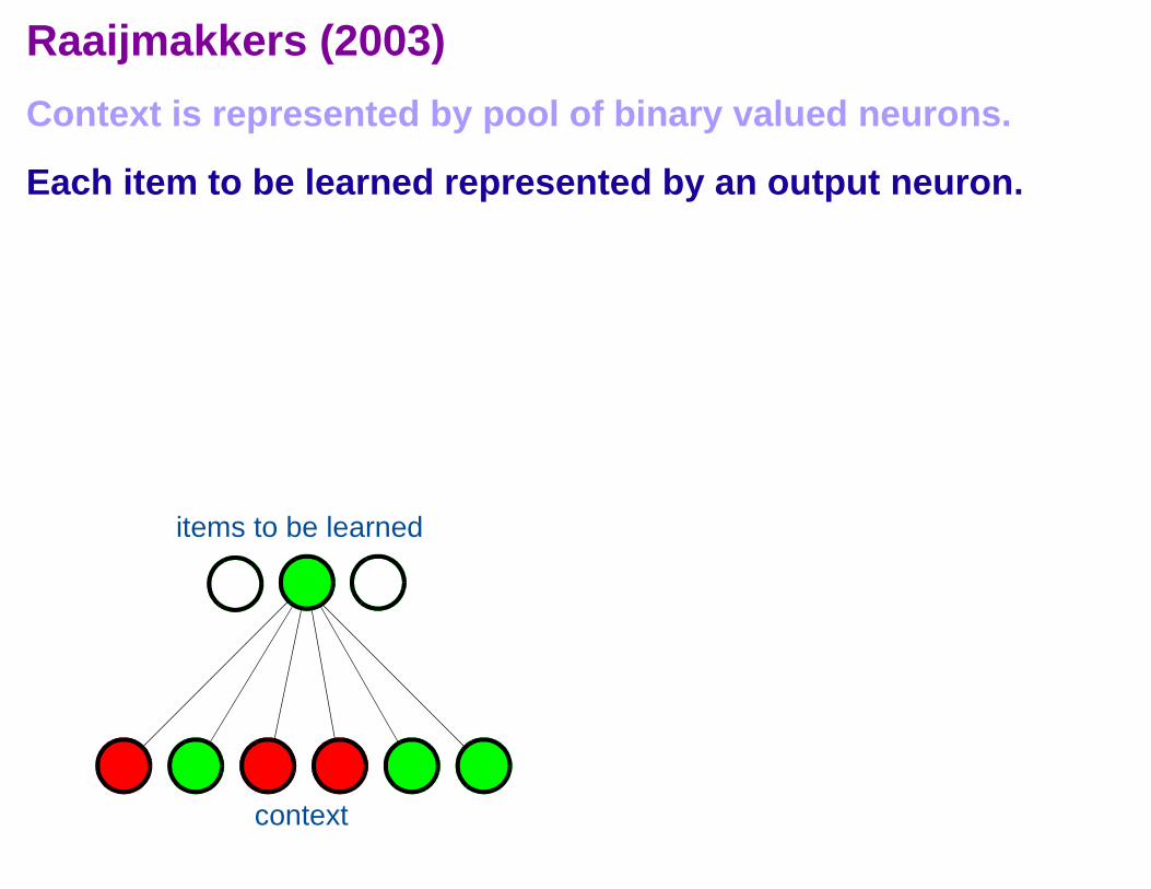
Raaijmakkers (2003)
Context is represented by pool of binary valued neu rons.
Each item to be learned represented by an output neu ron.
Hebbian learning rule
context
items to be learned

Raaijmakkers (2003)
Context is represented by pool of binary valued neu rons.
Each item to be learned represented by an output neu ron.
Hebbian learning rule
Output activity at test ~ recall probability
depends on similarity of study and test contexts
test contextstudy context

Raaijmakkers (2003)
Context is represented by pool of binary valued neu rons.
Each item to be learned represented by an output neu ron.
Hebbian learning rule
Output activity at test ~ recall probability
depends on similarity of study and test contexts
Spacing of study ⇒ context variability ⇒ robust recall
study 1 context study 2 context test context

Raaijmakkers (2003): Formal Description
Retrieval at test facilitated when context unit active at both study and test.
Expected output neuron activity ~ P(retrieval) ~ P(CS = 1 & CT = 1)

Raaijmakkers (2003): Formal Description
Retrieval at test facilitated when context unit active at both study and test.
Expected output neuron activity ~ P(retrieval) ~ P(CS = 1 & CT = 1)
How does context wander over time?
context bits flip from off to on at rate µ01
context bits flip from on to off at rate µ10
P(CS = 1 & CT = 1) = β2 + β(1–β) exp (– α RI)
flip rate: µ01 + µ10
retention interval
proportion on : µ01 / (µ01 + µ10)

What It Boils Down To
Forgetting function is exponential
0 10 20 30 40 50 60 70 80 90 100
Retention Interval
Re
trie
va
l P
rob
ab
ility

What It Boils Down To
Forgetting function is exponential
Human forgetting functions follow a power law(Wickelgren, 1974; Wixted & Carpenter, 2007):
P(retrieval) = λ(1 + ϕ RI)-φ
0 10 20 30 40 50 60 70 80 90 100
Retention Interval
Re
trie
va
l P
rob
ab
ility

What It Boils Down To
Forgetting function is exponential
Human forgetting functions follow a power law(Wickelgren, 1974; Wixted & Carpenter, 2007):
P(retrieval) = λ(1 + ϕ RI)-φ
Power law shows scale invariance
I.e., memory shows same properties at different time scales
0 10 20 30 40 50 60 70 80 90 100
Retention Interval
Re
trie
va
l P
rob
ab
ility
100
101
102
103
104
1010
109
108
107
106
105
104
103
102
101
100
Retention Interval
Re
trie
va
l P
rob
ab
ility

Is it a problem that Raaijmakkers’ (2003) model doe sn’t show scale invariance?
Yes, spacing effects are scale invariant.
Model has other problems too.
• Many free parameters and ugly hacks
• Doesn’t fit data particularly well

Predictive Utility Theories of Spacing Effects

Predictive Utility Theories of Spacing Effects
Suppose that memory• is limited in capacity, and/or• is imperfect and allows intrusions.
To achieve optimal performance, memories should be erased if they are not likely to be needed in the future.
eventoccurrence
time
eventoccurrence

Predictive Utility Theories of Spacing Effects
Suppose that memory• is limited in capacity, and/or• is imperfect and allows intrusions.
To achieve optimal performance, memories should be erased if they are not likely to be needed in the future.
eventoccurrence
time
eventoccurrence
test

Staddon, Chelaru, & Higa (2002)
Rats habituate to a repeated stream of stimuli.
Time for recovery from habituation ~ rate of stimul i
Longer-lasting memory for stimuli delivered at slower rate
...
...time

Staddon, Chelaru, & Higa (2002)
Each item to be learned represented by memory consis ting of leaky integrators at multiple time scales.
time
activity
integrator 1
time
integrator 2
time
integrator 3stimuli

Staddon, Chelaru, & Higa (2002)
Each item to be learned represented by memory consis ting of leaky integrators at multiple time scales.
Memory trace is the sum of the integrator activitie s.
time
activity
integrator 1
time
integrator 2
time
integrator 3stimuli

Staddon, Chelaru, & Higa (2002)
Each item to be learned represented by memory consis ting of leaky integrators at multiple time scales.
Memory trace is the sum of the integrator activitie s.
Memory storage rule
Integrators with long time constants get activated only when integrators with short time constants have decayed.
time
activity
integrator 1
time
integrator 2
time
integrator 3stimuli

Example
10 integrators
Stimulus repeatedly presented at various ISIs
Greater spacing ⇒ memory shifts to longer time-scale integrators ⇒ more durable memory
ISI 5
ISI 50
ISI 500
ISI 5000
Integrator Time Step

Example
10 integrators
Stimulus repeatedly presented at various ISIs
Greater spacing ⇒ memory shifts to longer time-scale integrators ⇒ more durable memory
Model is sensitive to predictive utility
Slower forgetting following longer ISI stimulus sequences.
ISI 5
ISI 50
ISI 500
ISI 5000
Integrator Time Step

Limitation of Staddon et al. Model
Model was evaluated only on rat habituation studies , which have many stimulus presentations.
Parameters not sufficiently well specified to model human spacing studies.

Two Models Share Two Key Properties
• Exponential decay of internal representations
• Learning rules for first study are identical
time
activity
integrator 1
time
integrator 2
time
integrator 3
0 10 20 30 40 50 60 70 80 90 100
Retention Interval
Re
trie
va
l P
rob
ab
ility
contextual drift(Raaijmakkers)
leaky integrators(Staddon et al.)

Integrating The Two Models
multiscale context model (MCM)
time
activity
integrator 1
time
integrator 2
time
integrator 3
contextual drift(Raaijmakkers)
multiscale representation(Staddon et al.)

Multiscale Context Model
In pool p, all units flip state at rate αp.
The pools can be different sizes:the relative proportion of units in pool p is γp.
pool 2 pool 3 pool N...pool 1

Multiscale Context Model
In pool p, all units flip state at rate αp.
The pools can be different sizes:the relative proportion of units in pool p is γp.
Forgetting function is a mixture of exponentials.
P(retrieval) ~
Mixture of exponentials are good approximations to human forgetting functions (Wixted).
pool 2 pool 3 pool N...pool 1
γpexp αpRI–( )p∑
+ + =

Forgetting Function
MCM forgetting function is more promising than Raaijmakkers’ forgetting function .
We can constraint MCM parameters, { αp} and { γp}, to replicate human forgetting functions.
0 10 20 30 40 50 60 70 80 90 100
Retention Interval
Re
trie
va
l P
rob
ab
ility

Picking Pool Size ( γ) and Rate ( α)

Picking Pool Size ( γ) and Rate ( α)αp = µ νp for
γp = ωp
MCM has four free parameters ( µ, ν, ω, + one more)
p 1 N,[ ]∈∈∈∈
1 10 20 30 40 500
0.05
0.1
0.15
0.2
pool1 10 20 30 40 50
0
0.02
0.04
0.06
0.08
0.1
pool

Multiscale Context Model: A Convergence of Theories

Multiscale Context Model: A Convergence of Theories
Raaijmakkers (2003)
Staddon et al. (2002)
context drift X
multipletime-scale
representationX
learning rule
X(dependence of
learning on retrieval success)
X(cascaded error
correction)

Multiscale Context Model: A Convergence of Theories
Raaijmakkers (2003)
Staddon et al. (2002)
Our Contribution
context drift X
multipletime-scale
representationX
learning rule
X(dependence of
learning on retrieval success)
X(cascaded error
correction)
variable pool size X
parameterization of multiscale
constantsX
neural characterization X
constrain parameters via
forgetting functionX
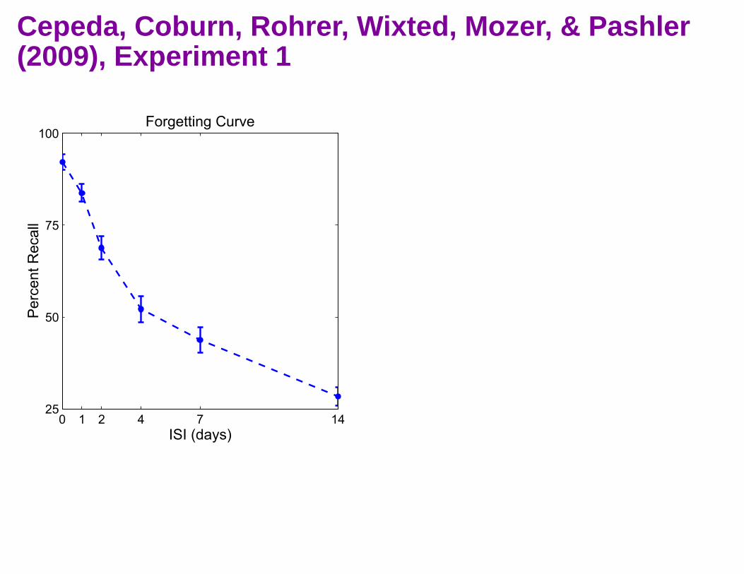
Cepeda, Coburn, Rohrer, Wixted, Mozer, & Pashler (2009), Experiment 1
0 1 2 4 7 1425
50
75
100Forgetting Curve
ISI (days)
Perc
ent R
ecall
0 1 2 4 7 1425
50
75
100
ISI (days)
Perc
ent R
ecall

Cepeda, Coburn, Rohrer, Wixted, Mozer, & Pashler (2009), Experiment 1
0 1 2 4 7 1425
50
75
100Forgetting Curve
ISI (days)
Perc
ent R
ecall
0 1 2 4 7 1425
50
75
100
ISI (days)
Perc
ent R
ecall

Cepeda, Coburn, Rohrer, Wixted, Mozer, & Pashler (2009), Experiment 1
0 1 2 4 7 1425
50
75
100Forgetting Curve
ISI (days)
Perc
ent R
ecall
0 1 2 4 7 1425
50
75
100Spacing Curve
ISI (days)
Perc
ent R
ecall
RI = 10 days

Cepeda, Coburn, Rohrer, Wixted, Mozer, & Pashler (2009), Experiment 1
0 1 2 4 7 1425
50
75
100Forgetting Curve
ISI (days)
Perc
ent R
ecall
0 1 2 4 7 1425
50
75
100Spacing Curve
ISI (days)
Perc
ent R
ecall
RI = 10 days

Cepeda, Coburn, Rohrer, Wixted, Mozer, & Pashler (2009), Experiment 1
0 1 2 4 7 1425
50
75
100Forgetting Curve
ISI (days)
Perc
ent R
ecall
0 1 2 4 7 1425
50
75
100Spacing Curve
ISI (days)
Perc
ent R
ecall
RI = 10 days
15 min spacing
1 day spacing
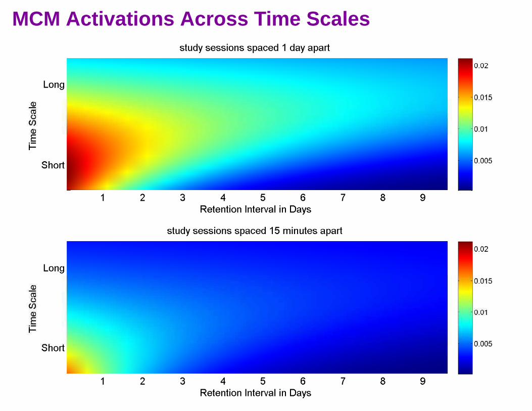
MCM Activations Across Time Scales

Cepeda, Coburn, Rohrer, Wixted, Mozer, & Pashler (2009), Experiment 2
7 28 84 1680
25
50
75
100Forgetting Curve
ISI (days)
Pe
rce
nt
Re
ca
ll
7 28 84 1680
25
50
75
100
ISI (days)P
erc
en
t R
eca
ll7 28 84 168
0
25
50
75
100
ISI (days)
Pe
rce
nt
Re
ca
ll
7 28 84 1680
25
50
75
100
ISI (days)
Pe
rce
nt
Re
ca
ll
7 28 84 1680
25
50
75
100
ISI (days)
Pe
rce
nt
Re
ca
ll
7 28 84 1680
25
50
75
100
ISI (days)
Pe
rce
nt
Re
ca
ll
facts
objects

Cepeda, Coburn, Rohrer, Wixted, Mozer, & Pashler (2009), Experiment 2
7 28 84 1680
25
50
75
100Forgetting Curve
ISI (days)
Pe
rce
nt
Re
ca
ll
7 28 84 1680
25
50
75
100Spacing Curve
ISI (days)P
erc
en
t R
eca
ll7 28 84 168
0
25
50
75
100
ISI (days)
Pe
rce
nt
Re
ca
ll
7 28 84 1680
25
50
75
100
ISI (days)
Pe
rce
nt
Re
ca
ll
7 28 84 1680
25
50
75
100
ISI (days)
Pe
rce
nt
Re
ca
ll
7 28 84 1680
25
50
75
100
ISI (days)
Pe
rce
nt
Re
ca
ll
RI = 168 days
RI = 168 days
facts
objects
Cepeda, Coburn, Rohrer, Wixted, Mozer, & Pashler (2009), Experiment 2
7 28 84 1680
25
50
75
100Forgetting Curve
ISI (days)
Pe
rce
nt
Re
ca
ll
7 28 84 1680
25
50
75
100Spacing Curve
ISI (days)P
erc
en
t R
eca
ll7 28 84 168
0
25
50
75
100Conditional Spacing Curve
ISI (days)
Pe
rce
nt
Re
ca
ll
7 28 84 1680
25
50
75
100
ISI (days)
Pe
rce
nt
Re
ca
ll
7 28 84 1680
25
50
75
100
ISI (days)
Pe
rce
nt
Re
ca
ll
7 28 84 1680
25
50
75
100
ISI (days)
Pe
rce
nt
Re
ca
ll
RI = 168 days
RI = 168 days
facts
objects
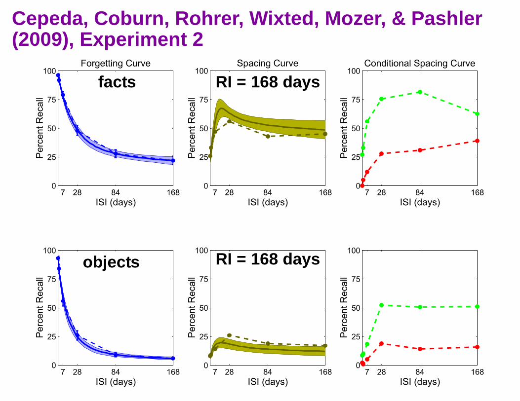

Cepeda, Vul, Rohrer, Wixted,& Pashler (2008)

17 21 35 70 1050
25
50
75
100Forgetting Curve
ISI (days)
Pe
rce
nt
Re
ca
ll
17 21 35 70 1050
25
50
75
100RI = 7
ISI (days)
Pe
rce
nt
Re
ca
ll
17 21 35 70 1050
25
50
75
100RI = 35
ISI (days)
Pe
rce
nt
Re
ca
ll
17 21 35 70 1050
25
50
75
100RI = 70
ISI (days)P
erc
en
t R
eca
ll
17 21 35 70 1050
25
50
75
100RI = 350
ISI (days)
Pe
rce
nt
Re
ca
ll
17 21 35 70 1050
25
50
75
100
ISI (days)
Pe
rce
nt
Re
ca
ll
17 21 35 70 1050
25
50
75
100
ISI (days)
Pe
rce
nt
Re
ca
ll
17 21 35 70 1050
25
50
75
100
ISI (days)
Pe
rce
nt
Re
ca
ll
17 21 35 70 1050
25
50
75
100
ISI (days)P
erc
en
t R
eca
ll
Cepeda, Vul, Rohrer, Wixted,& Pashler (2008)

17 21 35 70 1050
25
50
75
100Forgetting Curve
ISI (days)
Pe
rce
nt
Recall
17 21 35 70 1050
25
50
75
100RI = 7
ISI (days)
Pe
rce
nt
Re
ca
ll
17 21 35 70 1050
25
50
75
100RI = 35
ISI (days)
Pe
rce
nt
Re
ca
ll
17 21 35 70 1050
25
50
75
100RI = 70
ISI (days)P
erc
en
t R
eca
ll
17 21 35 70 1050
25
50
75
100RI = 350
ISI (days)
Pe
rce
nt
Re
ca
ll
17 21 35 70 1050
25
50
75
100
ISI (days)
Pe
rce
nt
Re
ca
ll
17 21 35 70 1050
25
50
75
100
ISI (days)
Pe
rce
nt
Re
ca
ll
17 21 35 70 1050
25
50
75
100
ISI (days)
Pe
rce
nt
Re
ca
ll
17 21 35 70 1050
25
50
75
100
ISI (days)P
erc
en
t R
eca
ll
Cepeda, Vul, Rohrer, Wixted,& Pashler (2008)

Why Are We Proposing Yet Another Model?
Previous models• have many free parameters, and• obtain only post hoc fits to data.
Our goal was to develop a truly predictive model.

Predicting Spacing Curve
MultiscaleContextModel
predictedrecall
intersessioninterval
characterizationof student
and domain

Predicting Spacing Curve
MultiscaleContextModel
predictedrecall
intersessioninterval
characterizationof student
and domain

Predicting Spacing Curve
MultiscaleContextModel1 7 14 21 35 70 105
0
20
40
60
80
100
Retention (Days)
% R
ecall
predictedrecall
forgetting afterone session
intersessioninterval

Predicting Spacing Curve
1 7 14 21 35 70 1050
20
40
60
80
100
spacing (days)
% r
eca
ll
7 day retention
35 day retention
70 day retention
350 day retention
Time Between Study Sessions (Days)
% R
ecal
l
MultiscaleContextModel1 7 14 21 35 70 105
0
20
40
60
80
100
Retention (Days)
% R
ecall
predictedrecall
Cepeda, Vul,Rohrer, Wixted, Pashler (2008)
forgetting afterone session
intersessioninterval

Beyond The Spacing Curve
predictedrecall
Multiscale
studyschedule
ContextModel1 7 14 21 35 70 105
0
20
40
60
80
100
Retention (Days)
% R
ecall
lag between session 1 and 2 = 10 dayslag between session 2 and 3 = 20 dayslag between session 3 and test = 50 days
forgetting afterone session

Beyond The Spacing Curve
predictedrecall
MultiscaleContextModel1 7 14 21 35 70 105
0
20
40
60
80
100
Retention (Days)
% R
ecall
optimalstudyschedule
OptimizationRoutine
forgetting afterone session
studyschedule

Beyond The Spacing Curve
predictedrecall
MultiscaleContextModel
forgetting afterone session
1 7 14 21 35 70 1050
20
40
60
80
100
Retention (Days)
% R
ecall
optimalstudyschedule
Student
feedbackOnline
OptimizationRoutine
studyschedule

Evaluating Optimal Scheduler In Simulation
Simulated student assumptions
• MCM is the correct model of human memory.
• Each item decays at a different rate for each student.
• Scheduler knows only the prior distribution over decay rates.
Optimal
Englishcue
Spanishresponse
Simulated
Scheduler
Student

Scheduler Simulation Details
Comparison of three schedulers
MCM-based
oldest first
worst first
session 1 session 2 test
time
session 3 session N. . .
1 week 2 weeks

Scheduler Simulation Results
15-25% boost in retention with optimal scheduling
10 11 12 13 14 15 160.2
0.3
0.4
0.5
0.6
0.7
0.8
# Study SessionsT
est
Re
ca
ll P
rop
ort
ion
300 Items, 30 Items Per Session
Oldest First
Worst First
MCM
10 20 30 40 50 60 700.2
0.3
0.4
0.5
0.6
0.7
0.8
0.9
1
# Items Per Session
Te
st
Re
ca
ll P
rop
ort
ion
300 Items, 10 Sessions
Oldest First
Worst First
MCM

Colorado Optimized Language Tutor (COLT)
Debugged in 2010-2011
Advanced business Spanish course at CU Boulder

Fall 2012
Experiment In Denver area middle school
Collaborator: Jeff Shroyer, member of The Educator Network
Second semester, 8th grade Spanish class, ~ 200 students

Fall 2012
Experiment In Denver area middle school
Collaborator: Jeff Shroyer, member of The Educator Network
Second semester, 8th grade Spanish class, ~ 200 students
Integrating COLT into curriculum
replacing currently used flashcard software
Shroyer restructuring class to do all vocabulary study + testing using COLT
blurs division between practice and quizzes
Focus on regular review
current software does not encourage review

Fall 2012
Within-student comparison of three scheduling algor ithms
• No review(but more time each week for study of new material)
• Generic review for all according to teacher’s current educational practice
• MCM selects customized review for each student
4 5 6 7
... ...
week

Individual Differences
Learning and retention is typically studied using p opulations of students and items.
But individual differences exist and are important.
Distribution of student scores(Japanese-English vocabulary)
Distribution of item scores(Lithuanian-English vocabulary)
0 0.2 0.4 0.6 0.8 10
2
4
6
8
10
Test Score
Fre
qu
en
cy
0 0.2 0.4 0.6 0.80
5
10
15
20
25
30
Test ScoreF
req
ue
ncy
Kang, Lindsey, Grimaldi, Pyc,& Rawson (2010Mozer, & Pashlr
(submitted)

Individual Differences
Learning and retention is typically studied using p opulations of students and items.
But individual differences exist and are important.
Challenge: infer a particular student’s state of kn owledge for a particular item from very weak feedback.
Distribution of student scores(Japanese-English vocabulary)
Distribution of item scores(Lithuanian-English vocabulary)
0 0.2 0.4 0.6 0.8 10
2
4
6
8
10
Test Score
Fre
qu
en
cy
0 0.2 0.4 0.6 0.80
5
10
15
20
25
30
Test ScoreF
req
ue
ncy
Kang, Lindsey, Grimaldi, Pyc,& Rawson (2010Mozer, & Pashlr
(submitted)

Item Response Theory
Traditional approach to modeling student and item e ffects in test taking (e.g., SATs)
Time invariant theory
δiαs
latent difficulty of item i
latent ability of student s
0
0.1
0.2
0.3
0.4
0.5
0.6
0.7
0.8
0.9
1
student ability – item difficulty
1
1 eδi αs–
+--------------------------
prob
abili
ty o
fco
rrec
t res
pons
e

Extending Item-Response Theory To Consider Time
• time to test
• number of study sessions
• spacing of sessions

Extending Item-Response Theory To Consider Time
• time to test
• number of study sessions
• spacing of sessions
See Lindsey paper
Considering study schedule yields significant improvement in ability to predict memory state of individual student for specific item.
Bayesian approach leverages data from population of students and items to make predictions about individuals
incorporate modelof memory and
forgetting
0 0.2 0.4 0.6 0.8 10
0.1
0.2
0.3
0.4
0.5
0.6
0.7
0.8
0.9
1
False Positive Rate
Tru
e P
ositiv
e R
ate
1PL (rasch)
1PL + power−law forgetting
global power−lawdynamic memory modelIRTIRT+ dynamic memory

Existing Flashcard Software
Many web sites, iPhone apps, etc.
studyblue.com flashcardexchange.comchinglish-online.com supermemo.orgspaced-ed.com mnemosyne-proj.orgsmart.fm ankitotalrecalllearning.com

Existing Flashcard Software
Many web sites, iPhone apps, etc.
studyblue.com flashcardexchange.comchinglish-online.com supermemo.orgspaced-ed.com mnemosyne-proj.orgsmart.fm ankitotalrecalllearning.com
All incorporate spacing based on some variant of heuristic system developed by Leitner (1972)
New flashcards start in bin 1
Cards tested correctly promoted to next bin.
Higher bins: longer lag before next review
Cards tested incorrectly demoted.
Goal: study card at the point of desireable difficulty (Bjork, 1994), i.e., when the individual is on the verge of forgetting.

Problems With Current Tools
• The point of desirable difficulty depends on speci fic individual, item, and study history.
Leitner box is ‘one size fits all’.
MCM can be tailored to the student, material, and even individual items.
• Optimal spacing depends on window of time over whi ch material needs to be accessible.
Therefore, can’t prescribe a study schedule without specifying the window.
MCM can optimize over any window.
Our conjecture
Precise quantitative predictions of forgetting for specific individual and item are needed to obtain the most benefit from a scheduler.

Why Hasn’t Cognitive Science Had A Greater Impact on Education?

Why Hasn’t Cognitive Science Had A Greater Impact on Education?
Most guidance is qualitative
“Space your study”
“The harder you work to learn, the better you’ll retain”
“Relate new material to be learned to learner’s existing knowledge”

Why Hasn’t Cognitive Science Had A Greater Impact on Education?
Most guidance is qualitative
“Space your study”
“The harder you work to learn, the better you’ll retain”
“Relate new material to be learned to learner’s existing knowledge”
Quantitative modeling and prediction can provide specific, customized, detailed guidance.
• particularly useful if there’s significant variability across individuals and materials

To Be Continued...
