theoretical motivations - mcgill university school of
TRANSCRIPT

Chapter 7
Theoretical Motivations
In this chapter, we will visit some of the theoretical underpinnings of graph neu-ral networks (GNNs). One of the most intriguing aspects of GNNs is that theywere independently developed from distinct theoretical motivations. From oneperspective, GNNs were developed based on the theory of graph signal process-ing, as a generalization of Euclidean convolutions to the non-Euclidean graphdomain [Bruna et al., 2014]. At the same time, however, neural message passingapproaches—which form the basis of most modern GNNs—were proposed byanalogy to message passing algorithms for probabilistic inference in graphicalmodels [Dai et al., 2016]. And lastly, GNNs have been motivated in severalworks based on their connection to the Weisfeiler-Lehman graph isomorphismtest [Hamilton et al., 2017b].
This convergence of three disparate areas into a single algorithm frameworkis remarkable. That said, each of these three theoretical motivations comes withits own intuitions and history, and the perspective one adopts can have a sub-stantial impact on model development. Indeed, it is no accident that we deferredthe description of these theoretical motivations until after the introduction ofthe GNN model itself. In this chapter, our goal is to introduce the key ideasunderlying these di↵erent theoretical motivations, so that an interested readeris free to explore and combine these intuitions and motivations as they see fit.
7.1 GNNs and Graph Convolutions
In terms of research interest and attention, the derivation of GNNs based onconnections to graph convolutions is the dominant theoretical paradigm. In thisperspective, GNNs arise from the question: How can we generalize the notionof convolutions to general graph-structured data?
75

76 CHAPTER 7. THEORETICAL MOTIVATIONS
7.1.1 Convolutions and the Fourier Transform
In order to generalize the notion of a convolution to graphs, we first must definewhat we wish to generalize and provide some brief background details. Letf and h be two functions. We can define the general continuous convolutionoperation ? as
(f ? h)(x) =
Z
Rd
f(y)h(x� y)dy. (7.1)
One critical aspect of the convolution operation is that it can be computed byan element-wise product of the Fourier transforms of the two functions:
(f ? h)(x) = F�1 (F(f(x)) � F(h(x))) , (7.2)
where
F(f(x)) = f(s) =
Z
Rd
f(x)e�2⇡x>sidx (7.3)
is the Fourier transform of f(x) and its inverse Fourier transform is defined as
F�1(f(s)) =
Z
Rd
f(s)e2⇡x>si
ds. (7.4)
In the simple case of univariate discrete data over a finite domain t 2{0, .., N � 1} (i.e., restricting to finite impulse response filters) we can simplifythese operations to a discrete circular convolution1
(f ?N h)(t) =N�1X
⌧=0
f(⌧)h((t� ⌧)mod N ) (7.5)
and a discrete Fourier transform (DFT)
sk =1pN
N�1X
t=0
f(xt)e� i2⇡
N kt (7.6)
=1pN
N�1X
t=0
f(xt)
✓cos
✓2⇡
Nkt
◆� isin
✓2⇡
Nkt
◆◆(7.7)
where sk 2 {s0..., sN�1} is the Fourier coe�cient corresponding to the se-quence (f(x0), f(x1), ..., f(xN�1)). In Equation (7.5) we use the notation ?N
to emphasize that this is a circular convolution defined over the finite domain{0, ..., N � 1}, but we will often omit this subscript for notational simplicity.
Interpreting the (discrete) Fourier transform The Fourier trans-form essentially tells us how to represent our input signal as a weightedsum of (complex) sinusoidal waves. If we assume that both the input data
1For simplicity, we limit ourselves to finite support for both f and h and define the boundarycondition using a modulus operator and circular convolution.

7.1. GNNS AND GRAPH CONVOLUTIONS 77
and its Fourier transform are real-valued, we can interpret the sequence[s0, s1, ..., sN�1] as the coe�cients of a Fourier series. In this view, sk tellsus the amplitude of the complex sinusoidal component e
� i2⇡N k, which has
frequency 2⇡kN (in radians). Often we will discuss high-frequency components
that have a large k and vary quickly as well as low-frequency componentsthat have k << N and vary more slowly. This notion of low and highfrequency components will also have an analog in the graph domain, wherewe will consider signals propagating between nodes in the graph.
In terms of signal processing, we can view the discrete convolution f ?h as afiltering operation of the series (f(x1), f(x2), ..., f(xN )) by a filter h. Generally,we view the series as corresponding to the values of the signal throughout time,and the convolution operator applies some filter (e.g., a band-pass filter) tomodulate this time-varying signal.
One critical property of convolutions, which we will rely on below, is the factthat they are translation (or shift) equivariant:
f(t+ a) ? g(t) = f(t) ? g(t+ a) = (f ? g)(t+ a). (7.8)
This property means that translating a signal and then convolving it by a filteris equivalent to convolving the signal and then translating the result. Note thatas a corollary convolutions are also equivariant to the di↵erence operation:
�f(t) ? g(t) = f(t) ?�g(t) = �(f ? g)(t), (7.9)
where�f(t) = f(t+ 1)� f(t) (7.10)
is the Laplace (i.e., di↵erence) operator on discrete univariate signals.These notions of filtering and translation equivariance are central to digital
signal processing (DSP) and also underlie the intuition of convolutional neu-ral networks (CNNs), which utilize a discrete convolution on two-dimensionaldata. We will not attempt to cover even a small fraction of the fields of digitalsignal processing, Fourier analysis, and harmonic analysis here, and we pointthe reader to various textbooks on these subjects [Grafakos, 2004, Katznelson,2004, Oppenheim et al., 1999, Rabiner and Gold, 1975].
7.1.2 From Time Signals to Graph Signals
In the previous section, we (briefly) introduced the notions of filtering and con-volutions with respect to discrete time-varying signals. We now discuss how wecan connect discrete time-varying signals with signals on a graph. Suppose wehave a discrete time-varying signal f(t0), f(t2), ..., f(tN�1). One way of viewingthis signal is as corresponding to a chain (or cycle) graph (Figure 7.1), whereeach point in time t is represented as a node and each function value f(t) rep-resents the signal value at that time/node. Taking this view, it is convenient torepresent the signal as a vector f 2 RN , with each dimension corresponding to

78 CHAPTER 7. THEORETICAL MOTIVATIONS
0…
1 N-2 N-1Figure 7.1: Representation of a (cyclic) time-series as a chain graph.
a di↵erent node in the chain graph. In other words, we have that f [t] = f(t)(as a slight abuse of notation). The edges in the graph thus represent how thesignal propagates; i.e., the signal propagates forward in time.2
One interesting aspect of viewing a time-varying signal as a chain graph isthat we can represent operations, such as time-shifts, using the adjacency andLaplacian matrices of the graph. In particular, the adjacency matrix for thischain graph corresponds to the circulant matrix Ac with
Ac[i, j] =
(1 if j = (i+ 1)mod N
0 otherwise,(7.11)
and the (unnormalized) Laplacian Lc for this graph can be defined as
Lc = I�Ac. (7.12)
We can then represent time shifts as multiplications by the adjacency matrix,
(Acf)[t] = f [(t+ 1)mod N ], (7.13)
and the di↵erence operation by multiplication by the Laplacian,
(Lcf)[t] = f [t]� f [(t+ 1)mod N ]. (7.14)
In this way, we can see that there is a close connection between the adjacencyand Laplacian matrices of a graph, and the notions of shifts and di↵erencesfor a signal. Multiplying a signal by the adjacency matrix propagates signalsfrom node to node, and multiplication by the Laplacian computes the di↵erencebetween a signal at each node and its immediate neighbors.
Given this graph-based view of transforming signals through matrix multi-plication, we can similarly represent convolution by a filter h as matrix multi-plication on the vector f :
(f ? h)(t) =N�1X
⌧=0
f(⌧)h(⌧ � t) (7.15)
= Qhf , (7.16)
2Note that we add a connection between the last and first nodes in the chain as a boundarycondition to keep the domain finite.

7.1. GNNS AND GRAPH CONVOLUTIONS 79
where Qh 2 RN⇥N is a matrix representation of the convolution operation byfilter function h and f = [f(t0), f(t2), ..., f(tN�1)]> is a vector representationof the function f . Thus, in this view, we consider convolutions that can berepresented as a matrix transformation of the signal at each node in the graph.3
Of course, to have the equality between Equation (7.15) and Equation (7.16),the matrix Qh must have some specific properties. In particular, we requirethat multiplication by this matrix satisfies translation equivariance, which cor-responds to commutativity with the circulant adjacency matrix Ac, i.e., werequire that
AcQh = QhAc. (7.17)
The equivariance to the di↵erence operator is similarly defined as
LcQh = QhLc. (7.18)
It can be shown that these requirements are satisfied for a real matrix Qh if
Qh = pN (Ac) =N�1X
i=0
↵iAic, (7.19)
i.e., if Qh is a polynomial function of the adjacency matrix Ac. In digital signalprocessing terms, this is equivalent to the idea of representing general filters aspolynomial functions of the shift operator [Ortega et al., 2018].4
Generalizing to general graphs
We have now seen how shifts and convolutions on time-varying discrete signalscan be represented based on the adjacency matrix and Laplacian matrix of achain graph. Given this view, we can easily generalize these notions to moregeneral graphs.
In particular, we saw that a time-varying discrete signal corresponds to achain graph and that the notion of translation/di↵erence equivariance corre-sponds to a commutativity property with adjacency/Laplacian of this chaingraph. Thus, we can generalize these notions beyond the chain graph by con-sidering arbitrary adjacency matrices and Laplacians. While the signal simplypropagates forward in time in a chain graph, in an arbitrary graph we might havemultiple nodes propagating signals to each other, depending on the structure ofthe adjacency matrix. Based on this idea, we can define convolutional filters ongeneral graphs as matrices Qh that commute with the adjacency matrix or theLaplacian.
More precisely, for an arbitrary graph with adjacency matrix A, we canrepresent convolutional filters as matrices of the following form:
Qh = ↵0I+ ↵1A+ ↵2A2 + ...+ ↵NAN
. (7.20)
3This assumes a real-valued filter h.4Note, however, that there are certain convolutional filters (e.g., complex-valued filters)
that cannot be represented in this way.

80 CHAPTER 7. THEORETICAL MOTIVATIONS
Intuitively, this gives us a spatial construction of a convolutional filter on graphs.In particular, if we multiply a node feature vector x 2 R|V | by such a convolutionmatrix Qh, then we get
Qhx = ↵0Ix+ ↵1Ax+ ↵2A2x+ ...+ ↵NANx, (7.21)
which means that the convolved signal Qhx[u] at each node u 2 V will corre-spond to some mixture of the information in the node’s N -hop neighborhood,with the ↵0, ...,↵N terms controlling the strength of the information comingfrom di↵erent hops.
We can easily generalize this notion of a graph convolution to higher dimen-sional node features. If we have a matrix of node features X 2 R|V|⇥m then wecan similarly apply the convolutional filter as
QhX = ↵0IX+ ↵1AX+ ↵2A2X+ ...+ ↵NANX. (7.22)
From a signal processing perspective, we can view the di↵erent dimensions ofthe node features as di↵erent “channels”.
Graph convolutions and message passing GNNs
Equation (7.22) also reveals the connection between the message passing GNNmodel we introduced in Chapter 5 and graph convolutions. For example, in thebasic GNN approach (see Equation 6.5) each layer of message passing essentiallycorresponds to an application of the simple convolutional filter
Qh = I+A (7.23)
combined with some learnable weight matrices and a non-linearity. In general,each layer of message passing GNN architecture aggregates information froma node’s local neighborhood and combines this information with the node’scurrent representation (see Equation 5.4). We can view these message passinglayers as a generalization of the simple linear filter in Equation (7.23), where weuse more complex non-linear functions. Moreover, by stacking multiple messagepassing layers, GNNs are able to implicitly operate on higher order polynomialsof the adjacency matrix.
The adjacency matrix, Laplacian, or a normalized variant? InEquation (7.22) we defined a convolution matrix Qh for arbitrary graphsas a polynomial of the adjacency matrix. Defining Qh in this way guar-antees that our filter commutes with the adjacency matrix, satisfying ageneralized notion of translation equivariance. However, in general com-mutativity with the adjacency matrix (i.e., translation equivariance) doesnot necessarily imply commutativity with the Laplacian L = D�A (or anyof its normalized variants). In this special case of the chain graph, we wereable to define filter matrices Qh that simultaneously commute with bothA and L, but for more general graphs we have a choice to make in terms

7.1. GNNS AND GRAPH CONVOLUTIONS 81
of whether we define convolutions based on the adjacency matrix or someversion of the Laplacian. Generally, there is no “right” decision in this case,and there can be empirical trade-o↵s depending on the choice that is made.Understanding the theoretical underpinnings of these trade-o↵s is an openarea of research [Ortega et al., 2018].
In practice researchers often use the symmetric normalized LaplacianLsym = D� 1
2LD� 12 or the symmetric normalized adjacency matrix Asym =
D� 12AD� 1
2 to define convolutional filters. There are two reasons why thesesymmetric normalized matrices are desirable. First, both these matriceshave bounded spectrums, which gives them desirable numerical stabilityproperties. In addition—and perhaps more importantly—these two ma-trices are simultaneously diagonalizable, which means that they share thesame eigenvectors. In fact, one can easily verify that there is a simplerelationship between their eigendecompositions, since
Lsym = I�Asym
)Lsym = U⇤U> Asym = U(I�⇤)U>
, (7.24)
where U is the shared set of eigenvectors and ⇤ is the diagonal matrixcontaining the Laplacian eigenvalues. This means that defining filters basedon one of these matrices implies commutativity with the other, which is avery convenient and desirable property.
7.1.3 Spectral Graph Convolutions
We have seen how to generalize the notion of a signal and a convolution to thegraph domain. We did so by analogy to some important properties of discreteconvolutions (e.g., translation equivariance), and this discussion led us to theidea of representing graph convolutions as polynomials of the adjacency matrix(or the Laplacian). However, one key property of convolutions that we ignoredin the previous subsection is the relationship between convolutions and theFourier transform. In this section, we will thus consider the notion of a spectralconvolution on graphs, where we construct graph convolutions via an extensionof the Fourier transform to graphs. We will see that this spectral perspectiverecovers many of the same results we previously discussed, while also revealingsome more general notions of a graph convolution.
The Fourier transform and the Laplace operator
To motivate the generalization of the Fourier transform to graphs, we rely onthe connection between the Fourier transform and the Laplace (i.e., di↵erence)operator. We previously saw a definition of the Laplace operator � in the caseof a simple discrete time-varying signal (Equation 7.10) but this operator can

82 CHAPTER 7. THEORETICAL MOTIVATIONS
be generalized to apply to arbitrary smooth functions f : Rd ! R as
�f(x) = r2f(x) (7.25)
=nX
i=1
@2f
@x2. (7.26)
This operator computes the divergence r of the gradient rf(x). Intuitively, theLaplace operator tells us the average di↵erence between the function value at apoint and function values in the neighboring regions surrounding this point.
In the discrete time setting, the Laplace operator simply corresponds to thedi↵erence operator (i.e., the di↵erence between consecutive time points). Inthe setting of general discrete graphs, this notion corresponds to the Laplacian,since by definition
(Lx)[i] =X
j2VA[i, j](x[i]� x[j]), (7.27)
which measures the di↵erence between the value of some signal x[i] at a nodei and the signal values of all of its neighbors. In this way, we can view theLaplacian matrix as a discrete analog of the Laplace operator, since it allows usto quantify the di↵erence between the value at a node and the values at thatnode’s neighbors.
Now, an extremely important property of the Laplace operator is that itseigenfunctions correspond to the complex exponentials. That is,
��(e2⇡ist) = �@2(e2⇡ist)
@t2= (2⇡s)2e2⇡ist, (7.28)
so the eigenfunctions of � are the same complex exponentials that make upthe modes of the frequency domain in the Fourier transform (i.e., the sinu-soidal plane waves), with the corresponding eigenvalue indicating the frequency.In fact, one can even verify that the eigenvectors u1, ...,un of the circulantLaplacian Lc 2 Rn⇥n for the chain graph are uj = 1p
n[1,!j ,!
2
j , ...,!nj ] where
!j = e2⇡jn .
The graph Fourier transform
The connection between the eigenfunctions of the Laplace operator and theFourier transform allows us to generalize the Fourier transform to arbitrarygraphs. In particular, we can generalize the notion of a Fourier transform byconsidering the eigendecomposition of the general graph Laplacian:
L = U⇤U>, (7.29)
where we define the eigenvectors U to be the graph Fourier modes, as a graph-based notion of Fourier modes. The matrix⇤ is assumed to have the correspond-ing eigenvalues along the diagonal, and these eigenvalues provide a graph-basednotion of di↵erent frequency values. In other words, since the eigenfunctions of
7.1. GNNS AND GRAPH CONVOLUTIONS 83
the general Laplace operator correspond to the Fourier modes—i.e., the com-plex exponentials in the Fourier series—we define the Fourier modes for a generalgraph based on the eigenvectors of the graph Laplacian.
Thus, the Fourier transform of signal (or function) f 2 R|V| on a graph canbe computed as
s = U>f (7.30)
and its inverse Fourier transform computed as
f = Us. (7.31)
Graph convolutions in the spectral domain are defined via point-wise productsin the transformed Fourier space. In other words, given the graph Fouriercoe�cients U>f of a signal f as well as the graph Fourier coe�cients U>h ofsome filter h, we can compute a graph convolution via element-wise productsas
f ?G h = U�U>f �U>h
�, (7.32)
where U is the matrix of eigenvectors of the Laplacian L and where we haveused ?G to denote that this convolution is specific to a graph G.
Based on Equation (7.32), we can represent convolutions in the spectraldomain based on the graph Fourier coe�cients ✓h = U>h 2 R|V| of the functionh. For example, we could learn a non-parametric filter by directly optimizing✓h and defining the convolution as
f ?G h = U�U>f � ✓h
�(7.33)
= (Udiag(✓h)U>)f (7.34)
where diag(✓h) is matrix with the values of ✓h on the diagonal. However, a filterdefined in this non-parametric way has no real dependency on the structureof the graph and may not satisfy many of the properties that we want from aconvolution. For example, such filters can be arbitrarily non-local.
To ensure that the spectral filter ✓h corresponds to a meaningful convolutionon the graph, a natural solution is to parameterize ✓h based on the eigenvaluesof the Laplacian. In particular, we can define the spectral filter as pN (⇤), sothat it is a degree N polynomial of the eigenvalues of the Laplacian. Definingthe spectral convolution in this way ensures our convolution commutes with theLaplacian, since
f ?G h = (UpN (⇤)U>)f (7.35)
= pN (L)f . (7.36)
Moreover, this definition ensures a notion of locality. If we use a degree k
polynomial, then we ensure that the filtered signal at each node depends oninformation in its k-hop neighborhood.
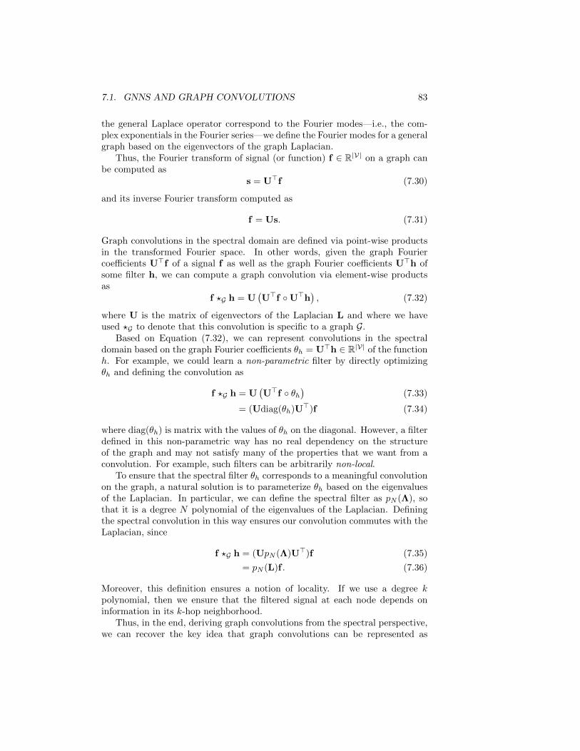
Thus, in the end, deriving graph convolutions from the spectral perspective,we can recover the key idea that graph convolutions can be represented as

84 CHAPTER 7. THEORETICAL MOTIVATIONS
polynomials of the Laplacian (or one of its normalized variants). However, thespectral perspective also reveals more general strategies for defining convolutionson graphs.
Interpreting the Laplacian eigenvectors as frequencies In the stan-dard Fourier transform we can interpret the Fourier coe�cients as corre-sponding to di↵erent frequencies. In the general graph case, we can nolonger interpret the graph Fourier transform in this way. However, we canstill make analogies to high frequency and low frequency components. Inparticular, we can recall that the eigenvectors ui, i = 1, ..., |V| of the Lapla-cian solve the minimization problem:
minui2R|V|:ui?uj8j<iu>i Lui
u>i uj
(7.37)
by the Rayleigh-Ritz Theorem. And we have that
u>i Lui =
1
2
X
u,v2VA[u, v](ui[u]� ui[v])
2 (7.38)
by the properties of the Laplacian discussed in Chapter 1. Together thesefacts imply that the smallest eigenvector of the Laplacian corresponds to asignal that varies from node to node by the least amount on the graph, thesecond smallest eigenvector corresponds to a signal that varies the secondsmallest amount, and so on. Indeed, we leveraged these properties of theLaplacian eigenvectors in Chapter 1 when we performed spectral clustering.In that case, we showed that the Laplacian eigenvectors can be used toassign nodes to communities so that we minimize the number of edges thatgo between communities. We can now interpret this result from a signalprocessing perspective: the Laplacian eigenvectors define signals that varyin a smooth way across the graph, with the smoothest signals indicatingthe coarse-grained community structure of the graph.
7.1.4 Convolution-Inspired GNNs
The previous subsections generalized the notion of convolutions to graphs. Wesaw that basic convolutional filters on graphs can be represented as polynomialsof the (normalized) adjacency matrix or Laplacian. We saw both spatial andspectral motivations of this fact, and we saw how the spectral perspective canbe used to define more general forms of graph convolutions based on the graphFourier transform. In this section, we will briefly review how di↵erent GNNmodels have been developed and inspired based on these connections.
7.1. GNNS AND GRAPH CONVOLUTIONS 85
Purely convolutional approaches
Some of the earliest work on GNNs can be directly mapped to the graph convo-lution definitions of the previous subsections. The key idea in these approachesis that they use either Equation (7.34) or Equation (7.35) to define a convo-lutional layer, and a full model is defined by stacking and combining multipleconvolutional layers with non-linearities. For example, in early work Brunaet al. [2014] experimented with the non-parametric spectral filter (Equation7.34) as well as a parametric spectral filter (Equation 7.35), where they definedthe polynomial pN (⇤) via a cubic spline approach. Following on this work,De↵errard et al. [2016] defined convolutions based on Equation 7.35 and definedpN (L) using Chebyshev polynomials. This approach benefits from the fact thatChebyshev polynomials have an e�cient recursive formulation and have variousproperties that make them suitable for polynomial approximation [Mason andHandscomb, 2002]. In a related approach, Liao et al. [2019b] learn polynomialsof the Laplacian based on the Lanczos algorithm.
There are also approaches that go beyond real-valued polynomials of theLaplacian (or the adjacency matrix). For example, Levie et al. [2018] considerCayley polynomials of the Laplacian and Bianchi et al. [2019] consider ARMAfilters. Both of these approaches employ more general parametric rational com-plex functions of the Laplacian (or the adjacency matrix).
Graph convolutional networks and connections to message passing
In their seminal work, Kipf and Welling [2016a] built o↵ the notion of graphconvolutions to define one of the most popular GNN architectures, commonlyknown as the graph convolutional network (GCN). The key insight of the GCNapproach is that we can build powerful models by stacking very simple graphconvolutional layers. A basic GCN layer is defined in Kipf and Welling [2016a]as
H(k) = �
⇣AH(k�1)W(k)
⌘, (7.39)
where A = (D+ I)�12 (I+A)(D+ I)�
12 is a normalized variant of the adjacency
matrix (with self-loops) and W(k) is a learnable parameter matrix. This modelwas initially motivated as a combination of a simple graph convolution (basedon the polynomial I+A), with a learnable weight matrix, and a non-linearity.
As discussed in Chapter 5 we can also interpret the GCN model as a vari-ation of the basic GNN message passing approach. In general, if we considercombining a simple graph convolution defined via the polynomial I + A withnon-linearities and trainable weight matrices we recover the basic GNN:
H(k) = �
⇣AH(k�1)W(k)
neigh+H(k�1)W(k)
self
⌘. (7.40)
In other words, a simple graph convolution based on I + A is equivalent toaggregating information from neighbors and combining that with information
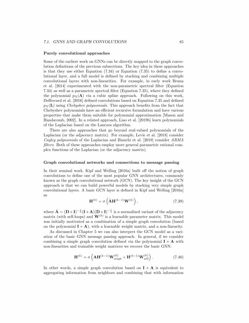
86 CHAPTER 7. THEORETICAL MOTIVATIONS
from the node itself. Thus we can view the notion of message passing as cor-responding to a simple form of graph convolutions combined with additionaltrainable weights and non-linearities.
Over-smoothing as a low-pass convolutional filter In Chapter 5 weintroduced the problem of over-smoothing in GNNs. The intuitive ideain over-smoothing is that after too many rounds of message passing, theembeddings for all nodes begin to look identical and are relatively unin-formative. Based on the connection between message-passing GNNs andgraph convolutions, we can now understand over-smoothing from the per-spective of graph signal processing.
The key intuition is that stacking multiple rounds of message passing ina basic GNN is analogous to applying a low-pass convolutional filter, whichproduces a smoothed version of the input signal on the graph. In particular,suppose we simplify a basic GNN (Equation 7.40) to the following updateequation:
H(k) = AsymH(k�1)W(k)
. (7.41)
Compared to the basic GNN in Equation (7.40), we have simplified themodel by removing the non-linearity and removing addition of the “self”embeddings at each message-passing step. For mathematical simplicityand numerical stability, we will also assume that we are using the sym-metric normalized adjacency matrix Asym = D� 1
2AD� 12 rather than the
unnormalized adjacency matrix. This model is similar to the simple GCNapproach proposed in Kipf and Welling [2016a] and essentially amounts totaking the average over the neighbor embeddings at each round of messagepassing.
Now, it is easy to see that after K rounds of message passing based onEquation (7.41), we will end up with a representation that depends on theKth power of the adjacency matrix:
H(K) = AKsym
XW, (7.42)
whereW is some linear operator andX is the matrix of input node features.To understand the connection between over-smoothing and convolutionalfilters, we just need to recognize that the multiplication AK
symX of the input
node features by a high power of the adjacency matrix can be interpretedas convolutional filter based on the lowest-frequency signals of the graphLaplacian.
For example, suppose we use a large enough value of K such that wehave reached the a fixed point of the following recurrence:
AsymH(K) = H(K)
. (7.43)
One can verify that this fixed point is attainable when using the normalizedadjacency matrix, since the dominant eigenvalue of Asym is equal to one.

7.1. GNNS AND GRAPH CONVOLUTIONS 87
We can see that at this fixed point, all the node features will have convergedto be completely defined by the dominant eigenvector of Asym, and moregenerally, higher powers of Asym will emphasize the largest eigenvaluesof this matrix. Moreover, we know that the largest eigenvalues of Asym
correspond to the smallest eigenvalues of its counterpart, the symmetricnormalized Laplacian Lsym (e.g., see Equation 7.24). Together, these factsimply that multiplying a signal by high powers of Asym corresponds to aconvolutional filter based on the lowest eigenvalues (or frequencies) of Lsym,i.e., it produces a low-pass filter!
Thus, we can see from this simplified model that stacking many roundsof message passing leads to convolutional filters that are low-pass, and—inthe worst case—these filters simply converge all the node representationsto constant values within connected components on the graph (i.e., the“zero-frequency” of the Laplacian).
Of course, in practice we use more complicated forms of message pass-ing, and this issue is partially alleviated by including each node’s previousembedding in the message-passing update step. Nonetheless, it is instruc-tive to understand how stacking “deeper” convolutions on graphs in a naiveway can actually lead to simpler, rather than more complex, convolutionalfilters.
GNNs without message passing
Inspired by connections to graph convolutions, several recent works have alsoproposed to simplify GNNs by removing the iterative message passing process.In these approaches, the models are generally defined as
Z = MLP✓ (f(A)MLP�(X)) , (7.44)
where f : RV|⇥|V| ! RV|⇥|V| is some deterministic function of the adjacency ma-trix A, MLP denotes a dense neural network, X 2 R|V|⇥m is the matrix of inputnode features, and Z 2 R|V|⇥d is the matrix of learned node representations.For example, in Wu et al. [2019], they define
f(A) = Ak, (7.45)
where A = (D+ I)�12 (A+ I)(D+ I)�
12 is the symmetric normalized adjacency
matrix (with self-loops added). In a closely related work Klicpera et al. [2019]defines f by analogy to the personalized PageRank algorithm as5
f(A) = ↵(I� (1� ↵)A)�1 (7.46)
= ↵
1X
k=0
⇣I� ↵A
⌘k. (7.47)
5Note that the equality between Equations (7.46) and (7.47) requires that the dominanteigenvalue of (I � ↵A) is bounded above by 1. In practice, Klicpera et al. [2019] use poweriteration to approximate the inversion in Equation (7.46).

88 CHAPTER 7. THEORETICAL MOTIVATIONS
The intuition behind these approaches is that we often do not need to interleavetrainable neural networks with graph convolution layers. Instead, we can simplyuse neural networks to learn feature transformations at the beginning and endof the model and apply a deterministic convolution layer to leverage the graphstructure. These simple models are able to outperform more heavily parameter-ized message passing models (e.g., GATs or GraphSAGE) on many classificationbenchmarks.
There is also increasing evidence that using the symmetric normalized ad-jacency matrix with self-loops leads to e↵ective graph convolutions, especiallyin this simplified setting without message passing. Both Wu et al. [2019] andKlicpera et al. [2019] found that convolutions based on A achieved the best em-pirical performance. Wu et al. [2019] also provide theoretical support for theseresults. They prove that adding self-loops shrinks the spectrum of correspondinggraph Laplacian by reducing the magnitude of the dominant eigenvalue. Intu-itively, adding self-loops decreases the influence of far-away nodes and makesthe filtered signal more dependent on local neighborhoods on the graph.
7.2 GNNs and Probabilistic Graphical Models
GNNs are well-understood and well-motivated as extensions of convolutions tograph-structured data. However, there are alternative theoretical motivationsfor the GNN framework that can provide interesting and novel perspectives.One prominent example is the motivation of GNNs based on connections tovariational inference in probabilistic graphical models (PGMs).
In this probabilistic perspective, we view the embeddings zu, 8u 2 V foreach node as latent variables that we are attempting to infer. We assume thatwe observe the graph structure (i.e., the adjacency matrix, A) and the inputnode features, X, and our goal is to infer the underlying latent variables (i.e.,the embeddings zv) that can explain this observed data. The message passingoperation that underlies GNNs can then be viewed as a neural network analogueof certain message passing algorithms that are commonly used for variationalinference to infer distributions over latent variables. This connection was firstnoted by Dai et al. [2016], and much of the proceeding discussions is basedclosely on their work.
Note that the presentation in this section assumes a substantial backgroundin PGMs, and we recommend Wainwright and Jordan [2008] as a good resourcefor the interested reader. However, we hope and expect that even a readerwithout any knowledge of PGMS can glean useful insights from the followingdiscussions.
7.2.1 Hilbert Space Embeddings of Distributions
To understand the connection between GNNs and probabilistic inference, wefirst (briefly) introduce the notion of embedding distributions in Hilbert spaces[Smola et al., 2007]. Let p(x) denote a probability density function defined

7.2. GNNS AND PROBABILISTIC GRAPHICAL MODELS 89
over the random variable x 2 Rm. Given an arbitrary (and possibly infinitedimensional) feature map � : Rm ! R, we can represent the density p(x)based on its expected value under this feature map:
µx =
Z
Rm
�(x)p(x)dx. (7.48)
The key idea with Hilbert space embeddings of distributions is that Equation(7.48) will be injective, as long as a suitable feature map � is used. This meansthat µx can serve as a su�cient statistic for p(x), and any computations wewant to perform on p(x) can be equivalently represented as functions of theembedding µx. A well-known example of a feature map that would guaranteethis injective property is the feature map induced by the Gaussian radial basisfunction (RBF) kernel [Smola et al., 2007].
The study of Hilbert space embeddings of distributions is a rich area ofstatistics. In the context of the connection to GNNs, however, the key takeawayis simply that we can represent distributions p(x) as embeddings µx in somefeature space. We will use this notion to motivate the GNN message passingalgorithm as a way of learning embeddings that represent the distribution overnode latents p(zv).
7.2.2 Graphs as Graphical Models
Taking a probabilistic view of graph data, we can assume that the graph struc-ture we are given defines the dependencies between the di↵erent nodes. Ofcourse, we usually interpret graph data in this way. Nodes that are connectedin a graph are generally assumed to be related in some way. However, in theprobabilistic setting, we view this notion of dependence between nodes in aformal, probabilistic way.
To be precise, we say that a graph G = (V, E) defines a Markov random field:
p({xv}, {zv}) /Y
v2V
�(xv, zv)Y
(u,v)2E
(zu, zv), (7.49)
where � and are non-negative potential functions, and where we use {xv} asa shorthand for the set {xv, 8v 2 V}. Equation (7.49) says that the distributionp({xv}, {zv}) over node features and node embeddings factorizes according tothe graph structure. Intuitively, �(xv, zv) indicates the likelihood of a nodefeature vector xv given its latent node embedding zv, while controls the de-pendency between connected nodes. We thus assume that node features aredetermined by their latent embeddings, and we assume that the latent embed-dings for connected nodes are dependent on each other (e.g., connected nodesmight have similar embeddings).
In the standard probabilistic modeling setting, � and are usually definedas parametric functions based on domain knowledge, and, most often, thesefunctions are assumed to come from the exponential family to ensure tractability[Wainwright and Jordan, 2008]. In our presentation, however, we are agnostic to
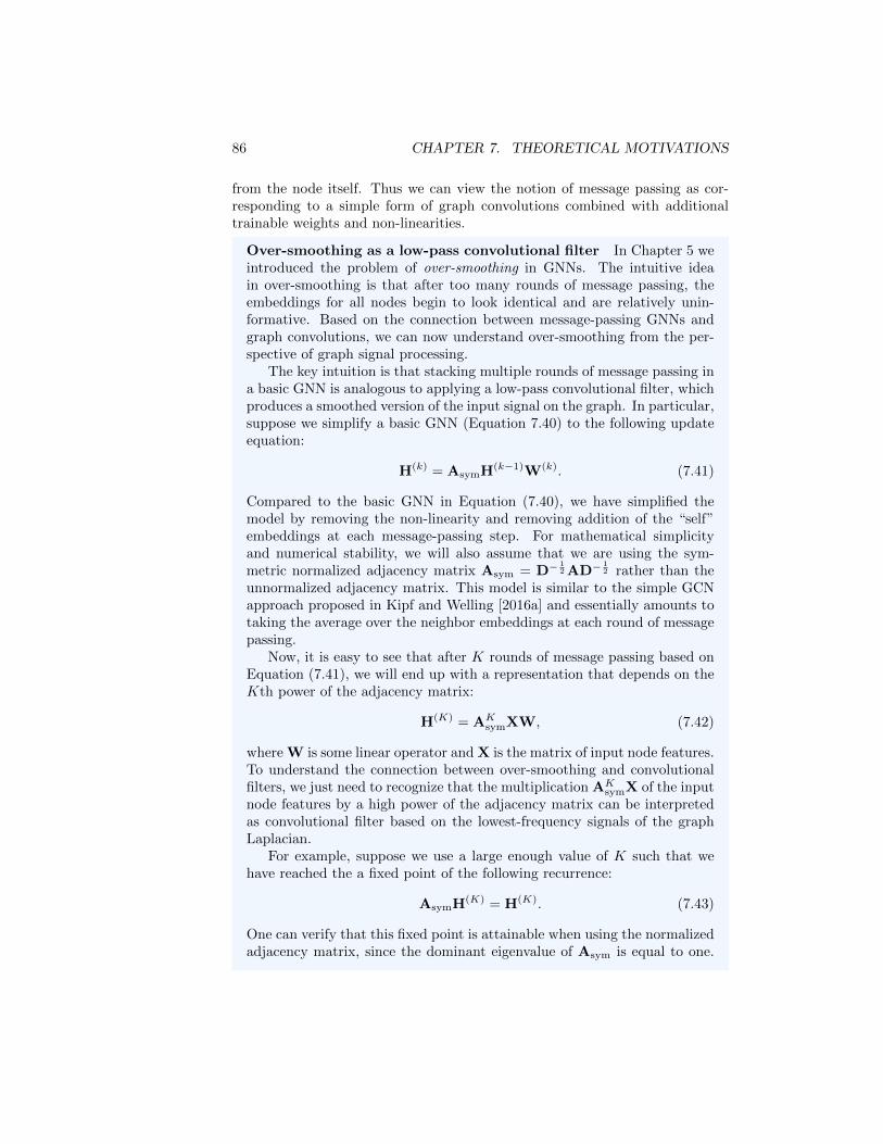
90 CHAPTER 7. THEORETICAL MOTIVATIONS
the exact form of � and , and we will seek to implicitly learn these functions byleveraging the Hilbert space embedding idea discussed in the previous section.
7.2.3 Embedding mean-field inference
Given the Markov random field defined by Equation (7.49), our goal is to inferthe distribution of latent embeddings p(zv) for all the nodes v 2 V , while alsoimplicitly learning the potential functions � and . In more intuitive terms ourgoal is to infer latent representations for all the nodes in the graph that canexplain the dependencies between the observed node features.
In order to do so, a key step is computing the posterior p({zv}|{xv}),i.e., computing the likelihood of a particular set of latent embeddings giventhe observed features. In general, computing this posterior is computationallyintractable—even if � and are known and well-defined—so we must resort toapproximate methods.
One popular approach—which we will leverage here—is to employ mean-fieldvariational inference, where we approximate the posterior using some functionsqv based on the assumption:
p({zv}|{xv}) ⇡ q({zv}) =Y
v2Vqv(zv), (7.50)
where each qv is a valid density. The key intuition in mean-field inference is thatwe assume that the posterior distribution over the latent variables factorizes intoV independent distributions, one per node.
To obtain approximating qv functions that are optimal in the mean-fieldapproximation, the standard approach is to minimize the Kullback–Leibler (KL)divergence between the approximate posterior and the true posterior:
KL(q({zv})|{p({zv}|{xv}) =Z
(Rd)V
Y
v2Vq({zv}) log
✓Qv2V q({zv})
p({zv}|{xv})
◆ Y
v2Vdzv.
(7.51)The KL divergence is one canonical way of measuring the distance betweenprobability distributions, so finding qv functions that minimize Equation (7.51)gives an approximate posterior that is as close as possible to the true poste-rior under the mean-field assumption. Of course, directly minimizing Equation(7.51) is impossible, since evaluating the KL divergence requires knowledge ofthe true posterior.
Luckily, however, techniques from variational inference can be used to showthat qv(zv) that minimize the KL must satisfy the following fixed point equa-tions:
log(q(zv)) = cv + log(�(xv, zv)) +X
u2N (v)
Z
Rd
qu(zu) log ( (zu, zv)) dzu,
(7.52)

7.2. GNNS AND PROBABILISTIC GRAPHICAL MODELS 91
where cv is a constant that does not depend on qv(zv) or zv. In practice, we can
approximate this fixed point solution by initializing some initial guesses q(t)v tovalid probability distributions and iteratively computing
log⇣q(t)v (zv)
⌘= cv + log(�(xv, zv)) +
X
u2N (v)
Z
Rd
q(t�1)
u (zu) log ( (zu, zv)) dzu.
(7.53)The justification behind Equation (7.52) is beyond the scope of this book. Forthe purposes of this book, however, the essential ideas are the following:
1. We can approximate the true posterior p({zv}|{xv}) over the latent em-beddings using the mean-field assumption, where we assume that theposterior factorizes into |V| independent distributions p({zv}|{xv}) ⇡Q
v2V qv(zv).
2. The optimal approximation under the mean-field assumption is given bythe fixed point in Equation (7.52), where the approximate posterior qv(zv)for each latent node embedding is a function of (i) the node’s feature zx and(ii) the marginal distributions qu(z)u, 8u 2 N (v) of the node’s neighbors’embeddings.
At this point the connection to GNNs begins to emerge. In particular, if weexamine the fixed point iteration in Equation (7.53), we see that the updated
marginal distribution q(t)v (zv) is a function of the node features xv (through
the potential function �) as well as function of the set of neighbor marginals
{q(t�1)
u (zu), 8u 2 N (v)} from the previous iteration (through the potential func-tion ). This form of message passing is highly analogous to the message passingin GNNs! At each step, we are updating the values at each node based on the setof values in the node’s neighborhood. The key distinction is that the mean-fieldmessage passing equations operate over distributions rather than embeddings,which are used in the standard GNN message passing.
We can make the connection between GNNs and mean-field inference eventighter by leveraging the Hilbert space embeddings that we introduced in Section7.2.1. Suppose we have some injective feature map � and can represent all themarginals qv(zv) as embeddings
µv =
Z
Rd
qv(zv)�(zv)dzv 2 Rd. (7.54)
With these representations, we can re-write the fixed point iteration in Equation(7.52) as
µ(t)v = c+ f(µ(t�1)
v ,xv, {µu, 8u 2 N (v)} (7.55)
where f is a vector-valued function. Notice that f aggregates information fromthe set of neighbor embeddings (i.e., {µu, 8u 2 N (v)} and updates the node’s
current representation (i.e., µ(t�1)
v ) using this aggregated data. In this way, wecan see that embedded mean-field inference exactly corresponds to a form ofneural message passing over a graph!
92 CHAPTER 7. THEORETICAL MOTIVATIONS
Now, in the usual probabilistic modeling scenario, we would define the po-tential functions � and , as well as the feature map �, using some domainknowledge. And given some �, , and we could then try to analyticallyderive the f function in Equation (7.55) that would allow us to work with anembedded version of mean field inference. However, as an alternative, we cansimply try to learn embeddings µv in and end-to-end fashion using some super-vised signals, and we can define f to be an arbitrary neural network. In otherwords, rather than specifying a concrete probabilistic model, we can simplylearn embeddings µv that could correspond to some probabilistic model. Basedon this idea, Dai et al. [2016] define f in an analogous manner to a basic GNNas
µ(t)v = �
0
@W(t)self
xv +W(t)neigh
X
u2N (v)
µ(t�1)
u
1
A . (7.56)
Thus, at each iteration, the updated Hilbert space embedding for node v is afunction of its neighbors’ embeddings as well as its feature inputs. And, as with
a basic GNN, the parameters W(t)self
and W(t)neigh
of the update process can betrained via gradient descent on any arbitrary task loss.
7.2.4 GNNs and PGMs More Generally
In the previous subsection, we gave a brief introduction to how a basic GNNmodel can be derived as an embedded form of mean field inference—a connec-tion first outlined by Dai et al. [2016]. There are, however, further ways toconnect PGMs and GNNs. For example, di↵erent variants of message passingcan be derived based on di↵erent approximate inference algorithms (e.g., Betheapproximations as discussed in Dai et al. [2016]), and there are also severalworks which explore how GNNs can be integrated more generally into PGMmodels [Qu et al., 2019, Zhang et al., 2020]. In general, the connections be-tween GNNs and more traditional statistical relational learning is a rich areawith vast potential for new developments.
7.3 GNNs and Graph Isomorphism
We have now seen how GNNs can be motivated based on connections to graphsignal processing and probabilistic graphical models. In this section, we willturn our attention to our third and final theoretical perspective on GNNs: themotivation of GNNs based on connections to graph isomorphism testing.
As with the previous sections, here we will again see how the basic GNNcan be derived as a neural network variation of an existing algorithm—in thiscase the Weisfieler-Lehman (WL) isomorphism algorithm. However, in additionto motivating the GNN approach, connections to isomorphism testing will alsoprovide us with tools to analyze the power of GNNs in a formal way.

7.3. GNNS AND GRAPH ISOMORPHISM 93
7.3.1 Graph Isomorphism
Testing for graph isomorphism is one of the most fundamental and well-studiedtasks in graph theory. Given a pair of graphs G1 and G2, the goal of graph iso-morphism testing is to declare whether or not these two graphs are isomorphic.In an intuitive sense, two graphs being isomorphic means that they are essen-tially identical. Isomorphic graphs represent the exact same graph structure,but they might di↵er only in the ordering of the nodes in their correspondingadjacency matrices. Formally, if we have two graphs with adjacency matricesA1 and A2, as well as node features X1 and X2, we say that two graphs areisomorphic if and only if there exists a permutation matrix P such that
PA1P> = A2 and PX1 = X2. (7.57)
It is important to note that isomorphic graphs are really are identical in terms oftheir underlying structure. The ordering of the nodes in the adjacency matrix isan arbitrary decision we must make when we represent a graph using algebraicobjects (e.g., matrices), but this ordering has no bearing on the structure of theunderlying graph itself.
Despite its simple definition, testing for graph isomorphism is a fundamen-tally hard problem. For instance, a naive approach to test for isomorphismwould involve the following optimization problem:
minP2PkPA1P> �A2k+ kPX1 �X2k
?= 0. (7.58)
This optimization requires searching over the full set of permutation matricesP to evaluate whether or not there exists a single permutation matrix P thatleads to an equivalence between the two graphs. The computational complexityof this naive approach is immense at O(|V |!), and in fact, no polynomial timealgorithm is known to correctly test isomorphism for general graphs.
Graph isomorphism testing is formally referred to as NP-indeterminate (NPI).It is known to not be NP-complete, but no general polynomial time algorithmsare known for the problem. (Integer factorization is another well-known prob-lem that is suspected to belong to the NPI class.) There are, however, manypractical algorithms for graph isomorphism testing that work on broad classesof graphs, including the WL algorithm that we introduced briefly in Chapter 1.
7.3.2 Graph Isomorphism and Representational Capacity
The theory of graph isomorphism testing is particularly useful for graph repre-sentation learning. It gives us a way to quantify the representational power ofdi↵erent learning approaches. If we have an algorithm—for example, a GNN—that can generate representations zG 2 Rd for graphs, then we can quantifythe power of this learning algorithm by asking how useful these representationswould be for testing graph isomorphism. In particular, given learned represen-tations zG1 and zG2 for two graphs, a “perfect” learning algorithm would havethat
zG1 = zG2 if and only if G1 is isomorphic to G2. (7.59)

94 CHAPTER 7. THEORETICAL MOTIVATIONS
1 3 2
11
A B C
DA
E F G
HE1,{3}⇢ A
1,{3}⇢ A
3,{1,1,2} ⇢ B
2,{3,1} ⇢ C
2,{3,1} ⇢ D
A,{B} ⇢ E
A,{B} ⇢ E
B,{A,A,C} ⇢ F
C,{B,D} ⇢ G
D,{C} ⇢ H
Iteration 0 Iteration 1 Iteration 2
Figure 7.2: Example of the WL iterative labeling procedure on one graph.
A perfect learning algorithm would generate identical embeddings for two graphsif and only if those two graphs were actually isomorphic.
Of course, in practice, no representation learning algorithm is going to be“perfect” (unless P=NP). Nonetheless, quantifying the power of a representationlearning algorithm by connecting it to graph isomorphism testing is very useful.Despite the fact that graph isomorphism testing is not solvable in general, we doknow several powerful and well-understood approaches for approximate isomor-phism testing, and we can gain insight into the power of GNNs by comparingthem to these approaches.
7.3.3 The Weisfieler-Lehman Algorithm
The most natural way to connect GNNs to graph isomorphism testing is basedon connections to the family of Weisfieler-Lehman (WL) algorithms. In Chapter1, we discussed the WL algorithm in the context of graph kernels. However, theWL approach is more broadly known as one of the most successful and well-understood frameworks for approximate isomorphism testing. The simplestversion of the WL algorithm—commonly known as the 1-WL—consists of thefollowing steps:
1. Given two graphs G1 and G2 we assign an initial label l(0)Gi(v) to each node
in each graph. In most graphs, this label is simply the node degree, i.e.,l(0)(v) = dv 8v 2 V , but if we have discrete features (i.e., one hot featuresxv) associated with the nodes, then we can use these features to definethe initial labels.
2. Next, we iteratively assign a new label to each node in each graph byhashing the multi-set of the current labels within the node’s neighborhood,as well as the node’s current label:
l(i)Gi(v) = HASH(l(i�1)
Gi(v), {{l(i�1)
Gi(u) 8u 2 N (v)}}), (7.60)
where the double-braces are used to denote a multi-set and the HASHfunction maps each unique multi-set to a unique new label.

7.3. GNNS AND GRAPH ISOMORPHISM 95
3. We repeat Step 2 until the labels for all nodes in both graphs converge, i.e.,
until we reach an iteration K where l(K)
Gj(v) = l
(K�1)
Gi(v), 8v 2 Vj , j = 1, 2.
4. Finally, we construct multi-sets
LGj = {{l(i)Gj(v), 8v 2 Vj , i = 0, ...,K � 1}}
summarizing all the node labels in each graph, and we declare G1 and G2
to be isomorphic if and only if the multi-sets for both graphs are identical,i.e., if and only if LG1 = LG2 .
Figure 7.2 illustrates an example of the WL labeling process on one graph. Ateach iteration, every node collects the multi-set of labels in its local neighbor-hood, and updates its own label based on this multi-set. After K iterationsof this labeling process, every node has a label that summarizes the structureof its K-hop neighborhood, and the collection of these labels can be used tocharacterize the structure of an entire graph or subgraph.
The WL algorithm is known to converge in at most |V| iterations and isknown to known to successfully test isomorphism for a broad class of graphs[Babai and Kucera, 1979]. There are, however, well known cases where the testfails, such as the simple example illustrated in Figure 7.3.
Figure 7.3: Example of two graphs that cannot be distinguished by the basicWL algorithm.
7.3.4 GNNs and the WL Algorithm
There are clear analogies between the WL algorithm and the neural messagepassing GNN approach. In both approaches, we iteratively aggregate infor-mation from local node neighborhoods and use this aggregated information toupdate the representation of each node. The key distinction between the twoapproaches is that the WL algorithm aggregates and updates discrete labels(using a hash function) while GNN models aggregate and update node embed-dings using neural networks. In fact, GNNs have been motivated and derivedas a continuous and di↵erentiable analog of the WL algorithm.
The relationship between GNNs and the WL algorithm (described in Section7.3.3) can be formalized in the following theorem:

96 CHAPTER 7. THEORETICAL MOTIVATIONS
Theorem 4 ([Morris et al., 2019, Xu et al., 2019]). Define a message-passingGNN (MP-GNN) to be any GNN that consists of K message-passing layers ofthe following form:
h(k+1)
u = UPDATE(k)
⇣h(k)u , AGGREGATE
(k)({h(k)v , 8v 2 N (u)})
⌘, (7.61)
where AGGREGATE is a di↵erentiable permutation invariant function and UPDATE
is a di↵erentiable function. Further, suppose that we have only discrete feature
inputs at the initial layer, i.e., h(0)
u = xu 2 Zd, 8u 2 V. Then we have that
h(K)
u 6= h(K)
v only if the nodes u and v have di↵erent labels after K iterationsof the WL algorithm.
In intuitive terms, Theorem 7.3.4 states that GNNs are no more powerful thanthe WL algorithm when we have discrete information as node features. If the WLalgorithm assigns the same label to two nodes, then any message-passing GNNwill also assign the same embedding to these two nodes. This result on nodelabeling also extends to isomorphism testing. If the WL test cannot distinguishbetween two graphs, then a MP-GNN is also incapable of distinguishing betweenthese two graphs. We can also show a more positive result in the other direction:
Theorem 5 ([Morris et al., 2019, Xu et al., 2019]). There exists a MP-GNN
such that h(K)
u = h(K)
v if and only if the two nodes u and v have the same labelafter K iterations of the WL algorithm.
This theorem states that there exist message-passing GNNs that are as powerfulas the WL test.
Which MP-GNNs are most powerful? The two theorems above statethat message-passing GNNs are at most as powerful as the WL algorithmand that there exist message-passing GNNs that are as powerful as the WLalgorithm. So which GNNs actually obtain this theoretical upper bound?Interestingly, the basic GNN that we introduced at the beginning of Chap-ter 5 is su�cient to satisfy this theory. In particular, if we define themessage passing updates as follows:
h(k)u = �
0
@W(k)self
h(k�1)
u +W(k)neigh
X
v2N (u)
h(k�1)
v + b(k)
1
A , (7.62)
then this GNN is su�cient to match the power of the WL algorithm [Morriset al., 2019].
However, most of the other GNN models discussed in Chapter 5 arenot as powerful as the WL algorithm. Formally, to be as powerful as theWL algorithm, the AGGREGATE and UPDATE functions need to be injective[Xu et al., 2019]. This means that the AGGREGATE and UPDATE operatorsneed to be map every unique input to a unique output value, which is notthe case for many of the models we discussed. For example, AGGREGATE
functions that use a (weighted) average of the neighbor embeddings are not

7.3. GNNS AND GRAPH ISOMORPHISM 97
injective; if all the neighbors have the same embedding then a (weighted)average will not be able to distinguish between input sets of di↵erent sizes.
Xu et al. [2019] provide a detailed discussion of the relative power ofvarious GNN architectures. They also define a “minimal” GNN model,which has few parameters but is still as powerful as the WL algorithm.They term this model the Graph Isomorphism Network (GIN), and it isdefined by the following update:
h(k)u = MLP
(k)
0
@(1 + ✏(k))h(k�1)
u +X
v2N (u)
h(k�1)
v
1
A , (7.63)
where ✏(k) is a trainable parameter.
7.3.5 Beyond the WL Algorithm
The previous subsection highlighted an important negative result regardingmessage-passing GNNs (MP-GNNs): these models are no more powerful thanthe WL algorithm. However, despite this negative result, investigating how wecan make GNNs that are provably more powerful than the WL algorithm is anactive area of research.
Relational pooling
One way to motivate provably more powerful GNNs is by considering the failurecases of the WL algorithm. For example, we can see in Figure 7.3 that the WLalgorithm—and thus all MP-GNNs—cannot distinguish between a connected6-cycle and a set of two triangles. From the perspective of message passing,this limitation stems from the fact that AGGREGATE and UPDATE operations areunable to detect when two nodes share a neighbor. In the example in Figure7.3, each node can infer from the message passing operations that they havetwo degree-2 neighbors, but this information is not su�cient to detect whethera node’s neighbors are connected to one another. This limitation is not simplya corner case illustrated in Figure 7.3. Message passing approaches generallyfail to identify closed triangles in a graph, which is a critical limitation.
To address this limitation, Murphy et al. [2019] consider augmenting MP-GNNs with unique node ID features. If we use MP-GNN(A,X) to denote anarbitrary MP-GNN on input adjacency matrix A and node features X, thenadding node IDs is equivalent to modifying the MP-GNN to the following:
MP-GNN(A,X� I), (7.64)
where I is the d ⇥ d-dimensional identity matrix and � denotes column-wisematrix concatenation. In other words, we simply add a unique, one-hot indicatorfeature for each node. In the case of Figure 7.3, adding unique node IDs would
98 CHAPTER 7. THEORETICAL MOTIVATIONS
allow a MP-GNN to identify when two nodes share a neighbor, which wouldmake the two graphs distinguishable.
Unfortunately, however, this idea of adding node IDs does not solve theproblem. In fact, by adding unique node IDs we have actually introduced anew and equally problematic issue: the MP-GNN is no longer permutationequivariant. For a standard MP-GNN we have that
P(MP-GNN(A,X)) = MP-GNN(PAP>,PX), (7.65)
where P 2 P is an arbitrary permutation matrix. This means that standardMP-GNNs are permutation equivariant. If we permute the adjacency matrixand node features, then the resulting node embeddings are simply permutedin an equivalent way. However, MP-GNNs with node IDs are not permutationinvariant since in general
P(MP-GNN(A,X� I)) 6= MP-GNN(PAP>, (PX)� I). (7.66)
The key issue is that assigning a unique ID to each node fixes a particular nodeordering for the graph, which breaks the permutation equivariance.
To alleviate this issue, Murphy et al. [2019] propose the Relational Pooling(RP) approach, which involves marginalizing over all possible node permuta-tions. Given any MP-GNN the RP extension of this GNN is given by
RP-GNN(A,X) =X
P2PMP-GNN(PAP>
, (PX)� I). (7.67)
Summing over all possible permutation matrices P 2 P recovers the permuta-tion invariance, and we retain the extra representational power of adding uniquenode IDs. In fact, Murphy et al. [2019] prove that the RP extension of a MP-GNN can distinguish graphs that are indistinguishable by the WL algorithm.
The limitation of the RP approach is in its computational complexity. Naivelyevaluating Equation (7.67) has a time complexity of O(|V|!), which is infeasiblein practice. Despite this limitation, however, Murphy et al. [2019] show thatthe RP approach can achieve strong results using various approximations todecrease the computation cost (e.g., sampling a subset of permutations).
The k-WL test and k-GNNs
The Relational Pooling (RP) approach discussed above can produce GNN mod-els that are provably more powerful than the WL algorithm. However, the RPapproach has two key limitations:
1. The full algorithm is computationally intractable.
2. We know that RP-GNNs are more powerful than the WL test, but wehave no way to characterize how much more powerful they are.
To address these limitations, several approaches have considered improvingGNNs by adapting generalizations of the WL algorithm.

7.3. GNNS AND GRAPH ISOMORPHISM 99
The WL algorithm we introduced in Section 7.3.3 is in fact just the simplestof what is known as the family of k-WL algorithms. In fact, the WL algorithmwe introduced previously is often referred to as the 1-WL algorithm, and itcan be generalized to the k-WL algorithm for k > 1. The key idea behind thek-WL algorithms is that we label subgraphs of size k rather than individualnodes. The k-WL algorithm generates representation of a graph G through thefollowing steps:
1. Let s = (u1, u2, ..., uk) 2 Vk be a tuple defining a subgraph of size k, where
u1 6= u2 6= ... 6= uk. Define the initial label l(0)G (s) for each subgraph bythe isomorphism class of this subgraph (i.e., two subgraphs get the samelabel if and only if they are isomorphic).
2. Next, we iteratively assign a new label to each subgraph by hashing themulti-set of the current labels within this subgraph’s neighborhood:
l(i)G (s) = HASH({{l(i�1)
G (s0), 8s0 2 Nj(s), j = 1, ..., k}}, l(i�1)
G (s)),
where the jth subgraph neighborhood is defined as
Nj(s) = {{(u1, ..., uj�1, v, uj+1, ..., uk), 8v 2 V}}. (7.68)
3. We repeat Step 2 until the labels for all subgraphs converge, i.e., until we
reach an iteration K where l(K)
G (s) = l(K�1)
G (s) for every k-tuple of nodess 2 Vk.
4. Finally, we construct a multi-set
LG = {{l(i)G (v), 8s 2 Vk, i = 0, ...,K � 1}}
summarizing all the subgraph labels in the graph.
As with the 1-WL algorithm, the summary LG multi-set generated by the k-WLalgorithm can be used to test graph isomorphism by comparing the multi-setsfor two graphs. There are also graph kernel methods based on the k-WL test[Morris et al., 2019], which are analogous to the WL-kernel introduced that wasin Chapter 1.
An important fact about the k-WL algorithm is that it introduces a hierarchyof representational capacity. For any k � 2 we have that the (k+1)-WL test isstrictly more powerful than the k-WL test.6 Thus, a natural question to ask iswhether we can design GNNs that are as powerful as the k-WL test for k > 2,and, of course, a natural design principle would be to design GNNs by analogyto the k-WL algorithm.
Morris et al. [2019] attempt exactly this: they develop a k-GNN approachthat is a di↵erentiable and continuous analog of the k-WL algorithm. k-GNNs
6However, note that running the k-WL requires solving graph isomorphism for graphsof size k, since Step 1 in the k-WL algorithm requires labeling graphs according to theirisomorphism type. Thus, running the k-WL for k > 3 is generally computationally intractable.

100 CHAPTER 7. THEORETICAL MOTIVATIONS
learn embeddings associated with subgraphs—rather than nodes—and the mes-sage passing occurs according to subgraph neighborhoods (e.g., as defined inEquation 7.68). Morris et al. [2019] prove that k-GNNs can be as expressive asthe k-WL algorithm. However, there are also serious computational concerns forboth the k-WL test and k-GNNs, as the time complexity of the message passingexplodes combinatorially as k increases. These computational concerns necessi-tate various approximations to make k-GNNs tractable in practice [Morris et al.,2019].
Invariant and equivariant k-order GNNs
Another line of work that is motivated by the idea of building GNNs that areas powerful as the k-WL test are the invariant and equivariant GNNs proposedby Maron et al. [2019]. A crucial aspect of message-passing GNNs (MP-GNNs;as defined in Theorem 7.3.4) is that they are equivariant to node permutations,meaning that
P(MP-GNN(A,X)) = MP-GNN(PAP>,PX). (7.69)
for any permutation matrix P 2 P. This equality says that that permuting theinput to an MP-GNN simply results in the matrix of output node embeddingsbeing permuted in an analogous way.
In addition to this notion of equivariance, we can also define a similar notionof permutation invariance for MP-GNNs at the graph level. In particular, MP-GNNs can be extended with a POOL : R|V|⇥d ! R function (see Chapter 5),which maps the matrix of learned node embeddings Z 2 R|V|⇥d to an embeddingzG 2 Rd of the entire graph. In this graph-level setting we have that MP-GNNsare permutation invariant, i.e.
POOL�MP-GNN(PAP>
,PX)�= POOL (MP-GNN(A,X)) , (7.70)
meaning that the pooled graph-level embedding does not change when di↵erentnode orderings are used.
Based on this idea of invariance and equivariance, Maron et al. [2019] proposea general form of GNN-like models based on permutation equivariant/invariant
tensor operations. Suppose we have an order-(k+1) tensor X 2 R|V|k⇥d, wherewe assume that the first k channels/modes of this tensor are indexed by thenodes of the graph. We use the notation P ? X to denote the operation wherewe permute the first k channels of this tensor according the node permutationmatrix P. We can then define an linear equivariant layer as a linear operator(i.e., a tensor) L : R|V|k1⇥d1 ! R|V|k2⇥d2 :
L⇥ (P ? X ) = P ? (L⇥ X ), 8P 2 P, (7.71)
where we use ⇥ to denote a generalized tensor product. Invariant linear opera-tors can be similarly defined as tensors L that satisfy the following equality:
L⇥ (P ? X ) = L⇥ X , 8P 2 P. (7.72)

7.3. GNNS AND GRAPH ISOMORPHISM 101
Note that both equivariant and invariant linear operators can be representedas tensors, but they have di↵erent structure. In particular, an equivariant oper-ator L : R|V|k⇥d1 ! R|V|k⇥d2 corresponds to a tensor L 2 R|V|2k⇥d1⇥d2 , whichhas 2k channels indexed by nodes (i.e., twice as many node channels as the in-
put). On the other hand, an invariant operator L : R|V|k⇥d1 ! Rd2 corresponds
to a tensor L 2 R|V|k⇥d1⇥d2 , which has k channels indexed by nodes (i.e., thesame number as the input). Interestingly, taking this tensor view of the linearoperators, the equivariant (Equation 7.71) and invariant (Equation 7.72) prop-erties for can be combined into a single requirement that the L tensor is a fixedpoint under node permutations:
P ? L = L, 8P 2 P. (7.73)
In other words, for a given input X 2 R|V |k⇥d, both equivariant and invariantlinear operators on this input will correspond to tensors that satisfy the fixedpoint in Equation (7.73), but the number of channels in the tensor will di↵erdepending on whether it is an equivariant or invariant operator.
Maron et al. [2019] show that tensors satisfying the the fixed point in Equa-tion (7.73) can be constructed as a linear combination of a set of fixed basiselements. In particular, any order-l tensor L that satisfies Equation (7.73) canbe written as
L = �1B1 + �2 + ...+ �b(l)Bb(l), (7.74)
where Bi are a set of fixed basis tensors, �i 2 R are real-valued weights, and b(l)is the lth Bell number. The construction and derivation of these basis tensorsis mathematically involved and is closely related to the theory of Bell numbersfrom combinatorics. However, a key fact and challenge is that the number ofbasis tensors needed grows with lth Bell number, which is an exponentiallyincreasing series.
Using these linear equivariant and invariant layers, Maron et al. [2019] de-fine their invariant k-order GNN model based on the following composition offunctions:
MLP � L0 � � � L1 � �L2 · · ·� � Lm ⇥ X . (7.75)
In this composition, we apply m equivariant linear layers L1, ...,Lm, whereLi : L : R|V|ki⇥d1 ! R|V|ki+1⇥d2 with maxi ki = k and k1 = 2. Between eachof these linear equivariant layers an element-wise non-linearity, denoted by �,is applied. The penultimate function in the composition, is an invariant linearlayer, L0, which is followed by a multi-layer perceptron (MLP) as the finalfunction in the composition. The input to the k-order invariant GNN is thetensor X 2 R|V|2⇥d, where the first two channels correspond to the adjacencymatrix and the remaining channels encode the initial node features/labels.
This approach is called k-order because the equivariant linear layers involvetensors that have up to k di↵erent channels. Most importantly, however, Maronet al. [2019] prove that k-order models following Equation 7.75 are equally pow-erful as the k-WL algorithm. As with the k-GNNs discussed in the previoussection, however, constructing k-order invariant models for k > 3 is generallycomputationally intractable.