Theoretical analysis of degradation mechanisms in the formation of morphogengradientsBehnaz Bozorgui, Hamid Teimouri, and Anatoly B. Kolomeisky Citation: The Journal of Chemical Physics 143, 025102 (2015); doi: 10.1063/1.4926461 View online: http://dx.doi.org/10.1063/1.4926461 View Table of Contents: http://scitation.aip.org/content/aip/journal/jcp/143/2?ver=pdfcov Published by the AIP Publishing Articles you may be interested in Development of morphogen gradient: The role of dimension and discreteness J. Chem. Phys. 140, 085102 (2014); 10.1063/1.4866453 Kinetics of receptor occupancy during morphogen gradient formation J. Chem. Phys. 138, 244105 (2013); 10.1063/1.4811654 Theoretical and experimental analysis of the forced LacI-AraC oscillator with a minimal gene regulatory model Chaos 23, 025109 (2013); 10.1063/1.4809786 Relationship of ORF length and mRNA degradation in Escherichia coli genome AIP Conf. Proc. 1479, 1560 (2012); 10.1063/1.4756461 Physical interpretation of mean local accumulation time of morphogen gradient formation J. Chem. Phys. 135, 154115 (2011); 10.1063/1.3654159

This article is copyrighted as indicated in the article. Reuse of AIP content is subject to the terms at: http://scitation.aip.org/termsconditions. Downloaded to IP:

128.42.226.167 On: Thu, 30 Jul 2015 17:20:48

THE JOURNAL OF CHEMICAL PHYSICS 143, 025102 (2015)

Theoretical analysis of degradation mechanisms in the formationof morphogen gradients

Behnaz Bozorgui, Hamid Teimouri, and Anatoly B. KolomeiskyDepartment of Chemistry and Center for Theoretical Biological Physics, Rice University,Houston, Texas 77005-1892, USA

(Received 3 April 2015; accepted 25 June 2015; published online 9 July 2015)

Fundamental biological processes of development of tissues and organs in multicellular organisms aregoverned by various signaling molecules, which are called morphogens. It is known that spatial andtemporal variations in the concentration profiles of signaling molecules, which are frequently referredas morphogen gradients, lead to a cell differentiation via activating specific genes in a concentration-dependent manner. It is widely accepted that the establishment of the morphogen gradients involvesmultiple biochemical reactions and diffusion processes. One of the critical elements in the formationof morphogen gradients is a degradation of signaling molecules. We develop a new theoreticalapproach that provides a comprehensive description of the degradation mechanisms. It is based onthe idea that the degradation works as an effective potential that drives the signaling molecules awayfrom the source region. Utilizing the method of first-passage processes, the dynamics of the formationof morphogen gradients for various degradation mechanisms is explicitly evaluated. It is found thatlinear degradation processes lead to a dynamic behavior specified by times to form the morphogengradients that depend linearly on the distance from the source. This is because the effective potentialdue to the degradation is quite strong. At the same time, nonlinear degradation mechanisms yield aquadratic scaling in the morphogen gradients formation times since the effective potentials are muchweaker. Physical-chemical explanations of these phenomena are presented. C 2015 AIP PublishingLLC. [http://dx.doi.org/10.1063/1.4926461]

I. INTRODUCTION

The development of multicellular organisms is one ofthe most important fundamental processes in nature.1–3 Themost critical question here is how a small set of geneticallyidentical cells in embryos can produce morphologically andfunctionally different tissues and organs in fully developedorganisms. The central concept of biological development isthat the observed complex spatial patterning is due to action ofsignaling molecules that are also called morphogens.1–8 Thesesignaling molecules can produce non-uniform concentrationprofiles, the so-called morphogen gradients, that via complexbiochemical networks stimulate or suppress specific genesin embryo cells, depending on their local concentrations. Inrecent years, there were multiple experimental and theoreticalinvestigations on how the morphogen gradients are created andhow they function. This led to several exciting discoveries inthe field.5–24 However, many aspects of the underlying mech-anisms that result in the formation of the signaling moleculesdensity profiles remain not fully explained.25

A large variety of approaches to describe the develop-ment of morphogen gradients have been proposed and dis-cussed.6,7,25 Many of them follow the original idea ofTuring that the morphogen gradients are resulting from com-plex reaction-diffusion process.26 The most popular and widelyutilized method to explain the formation of the signaling mole-cules profiles is known as a synthesis-diffusion-degradation(SDD) model.7,10,27 In this picture, the process starts withmorphogens being produced at specific localized regions in

the embryo, from which they diffuse along the cells. Signalingmolecules also can be removed from the system after bindingto specific receptors on cells. At large times, this leads toexponentially decaying concentration profiles which qualita-tively agree with many experimentally observed morphogengradients.7,9–12,27,28

It is widely accepted that the process of degradation orremoval of signaling molecules from the system is criticallyimportant for the development of morphogen gradients.7 Thisallows the formation of the stationary profiles of signalingmolecules, ensuring the robustness of the genetic informationtransfer in biological development. But specific details of howthe degradation influences the formation of morphogen gradi-ents are still not well clarified. There are many counter-intuitiveobservations that cannot be explained by current theoreticalviews. In the classical SDD model it is assumed that the degra-dation is linear, i.e., the particle flux leaving the system isproportional to the local concentration of morphogens. It wasshown theoretically that for this model the time to establishthe stationary morphogen gradient at a given location, whichis also known as a local accumulation time (LAT), is a linearfunction of the distance from the source.20 This observationis surprising since for the system with unbiased diffusion ofparticles much slower quadratic scaling was expected.20,22 Atthe same time, several experiments suggested that in somecases the establishment of morphogen gradients is associatedwith nonlinear degradation mechanisms when the presence ofsignaling molecules self-enhances or self-catalyzes its removalfrom the system.30–33 Theoretical investigations of temporal

0021-9606/2015/143(2)/025102/7/$30.00 143, 025102-1 © 2015 AIP Publishing LLC

This article is copyrighted as indicated in the article. Reuse of AIP content is subject to the terms at: http://scitation.aip.org/termsconditions. Downloaded to IP:

128.42.226.167 On: Thu, 30 Jul 2015 17:20:48

025102-2 Bozorgui, Teimouri, and Kolomeisky J. Chem. Phys. 143, 025102 (2015)

evolution of the morphogen gradients with nonlinear degrada-tion suggested that in this case the local accumulation times,in contrast to linear degradation, scale quadratically with thedistance from the source.30 But the presented mathematicalanalysis was rather very complicated, and only bounds for LATin several cases were obtained.30

These observations raised several interesting and impor-tant questions concerning the role of the degradation in regulat-ing the concentration profiles of signaling molecules. Why thedegradation accelerates the relaxation to the stationary state forthe linear degradation? Why the actions of linear and nonlineardegradation processes are so different? What is the physicalmechanism of degradation? Recently, one of us proposed anidea that might resolve some of these issues.22 It was suggestedthat the degradation acts as an effective potential that pushessignaling molecules away from the source region. It means thatthe degradation will make the diffusion of morphogen mole-cules effectively biased. However, only qualitative argumentshave been presented.

In this paper, we extend and generalize the original ideathat the removal of signaling molecules works as the effec-tive potential. A new quantitative approach that provides amicroscopic view on the role of degradation in the formationof morphogen gradients is developed. It allows us to explainthe differences between various degradation mechanisms. Weargue that the linear degradation corresponds to a strong poten-tial, leading to strongly biased motion of the signaling mole-cules. At the same time, the non-linear degradation creates apotential that is too weak to modify the underlying random-walk scaling behavior of the system, affecting only the magni-tude of fluctuations.

II. THEORETICAL METHOD

Let us start the analysis of degradation mechanisms byintroducing a discrete SDD model as presented in Fig. 1(a).The cells in the embryo are represented as discrete sites n

FIG. 1. (a) Schematic view of a discrete synthesis-diffusion-degradationmodel with unbiased diffusion. (b) Schematic view of equivalent biased-diffusion model without degradation and with modified diffusion rates. Lat-tice sites correspond to embryo cells.

≥ 0 on this semi-infinite lattice. The signaling molecules areproduced at the origin (n = 0) with a rate Q. Then morphogensdiffuse along the lattice with a diffusion constant D. At eachlattice site n, the molecule can be degraded with a rate kn.It is convenient to adopt a single-molecule view of the pro-cess where the local concentration of signaling molecules isproportional to a probability to find a morphogen molecule at agiven location.22,29 One can define then Pn(t) as a probability offinding the morphogen at the site n at time t. These probabilitiesevolve with time as described by a set of master equations,

dPn(t)dt

= DPn+1(t) + DPn−1(t) − (2D + kn)Pn(t), (1)

for n > 0; while at the origin (n = 0) we have

dP0(t)dt

= Q + DP1(t) − (D + k0)P0(t). (2)

The situation when the degradation rate kn is independentof the concentration of signaling molecules corresponds tolinear degradation since the total flux that removes morpho-gens from the system [knPn(t)] is proportional to the concen-tration. For the case of constant kn = k, this discrete SDDmodel with linear degradation was fully analyzed before.22 Ina more general scenario, the degradation rate might dependon the local concentration, kn = kPm−1

n , where a parameter mspecifies the degree of non-linearity, and this corresponds tonon-linear degradation processes. However, it is not feasiblegenerally to obtain full analytic solutions for these non-lineardegradation models (with m > 1).

The main idea of our approach is that degradation acts asan effective potential. This suggests that the original reaction-diffusion process with degradation is equivalent to a biaseddiffusion process in such potential but without degradation, asshown in Fig. 1(b). To explain the origin of this potential, let usconsider the system in the steady-state limit when a stationarynon-uniform profile P(s)

n is achieved. The degradation leads to aconcentration gradient between any two consecutive sites, andthis gradient can be associated with a difference in the chemicalpotentials of the morphogens,

µn+1 − µn = kBT ln P(s)n+1 − kBT ln P(s)

n . (3)

This can also be viewed as an effective potential that influencesparticles that are not degraded. It follows then that this potentialcan be evaluated as

Ueffn = kBT ln P(s)

n . (4)

It is important to note that our system is non-equilibrium sothat equilibrium concepts cannot be applied here. There is aflux of signaling molecules moving in the positive direction(see Fig. 1(a)). This is analogous to having a potential actingon morphogens pushing them away from the origin.

The above arguments indicate that dynamics of a reaction-diffusion model (Fig. 1(a)) can be approximated by a biased-diffusion model (see Fig. 1(b)), which is much simpler toanalyze. We assume that the biased-diffusion model has L(L → ∞) sites, and the molecule starts at the origin at t = 0.The particle hops to the right, and when it reaches the lastsite n = L it instantaneously moves back to the origin n = 0.For the equivalent biased-diffusion model, we define Πn(t) as

This article is copyrighted as indicated in the article. Reuse of AIP content is subject to the terms at: http://scitation.aip.org/termsconditions. Downloaded to IP:

128.42.226.167 On: Thu, 30 Jul 2015 17:20:48

025102-3 Bozorgui, Teimouri, and Kolomeisky J. Chem. Phys. 143, 025102 (2015)

the probability of finding a particle at position n at time t.These probabilities are also governed by corresponding masterequations,

dΠn(t)dt

= rn+1Πn+1(t) + gn−1Πn−1(t) − (rn + gn)Πn(t), (5)

for 0 < n < L, while for n = 0 and n = L, we have

dΠ0(t)dt

= J + r1Π1(t) − g0Π0(t), (6)

dΠL(t)dt

= gL−1ΠL−1(t) − rLΠL(t) − J, (7)

where J is the flux from the site L back to the origin n = 0.At large times, the system reaches the stationary state withthe constant flux J across every site. One can also see thequalitative difference between two models. While the SDDmodel achieves the conservation of probability only at thestationary state, the biased-diffusion model always conservesthe probability. Based on these observations, we expect thatthe mapping between two models should work better at largetimes, approaching the stationary state.

The diffusion rates gn and rn in the biased-diffusion modelare related to each other via changes in the effective potential.This can be shown using the detailed balance arguments,34

gnrn+1

= exp *,

Ueffn −Ueff

n+1

kBT+-. (8)

It is important to note that we do not assume the detailedbalance here because the system is out of equilibrium. Butthese arguments tell us that the detailed balance is restoredwhen the system reaches the equilibrium for Ueff

n = Ueffn+1, and

the transition rates in both directions become equal, i.e., gn= rn+1. This is a crucial result because it directly couplesthe original SDD model with degradation to the new biased-diffusion model without degradation.

One more step is needed in order to have comparable dy-namic behaviors in both models. The average residence timesfor the particles at each site provide a measure of relevant timescales in the system. It seems reasonable to require that thesequantities to be the same in both models, leading to

gn + rn = 2D + kn. (9)

Note that Eqs. (8) and (9) uniquely define the forward andbackward rates in the biased-diffusion model.

To understand the mechanisms of formation of morpho-gen gradients, the relaxation dynamics to a stationary-statebehavior needs to be investigated. This can be done by analyz-ing the local accumulation times tn, which are defined as timesto reach the stationary-state concentration at the given positionn. The general approach for computing LAT is known,20 butanalytical results can only be obtained for the linear degra-dation model (m = 1). We propose to use mean first-passagetimes τn (MFPT), which are defined as times to reach a givensite for the first time, as a measure of dynamics of establishingthe morphogen gradients. It was shown before that MFPTapproximate very well LAT at large distances from the source,i.e., for large n.22,35 In addition, the first-passage analysis pro-vides a clear physical view of the underlying phenomena in thedevelopment of morphogen gradients.

Thus, our method of evaluating the formation of signalingmolecules profiles consists of three steps. First, from the orig-inal SDD model with degradation the stationary-state profilesare obtained, from which the effective potentials are explicitlyevaluated. In the second step, the transition rates in the equiva-lent biased-diffusion model without degradation are computed.Finally, these rates are utilized for calculating the first-passagedynamics as a way of describing the approach to the stationary-state behavior in the system. It is important to note here that thisprocedure is not exact since it involves several approximations.

III. LINEAR DEGRADATION

To test our theoretical approach, we start with the simplestlinear degradation model where all dynamic properties areanalytically calculated for all sets of parameters.20,22 Thestationary-state profile for the SDD model can be easily eval-uated,22

P(s)n =

2Qxn

k +√

k2 + 4Dk, (10)

with x = (2D + k −√

k2 + 4kD)/2D. This expressions allowsus to estimate the effective potential due to degradation for theequivalent biased-diffusion model,

Ueffn

kBT≃ n ln x. (11)

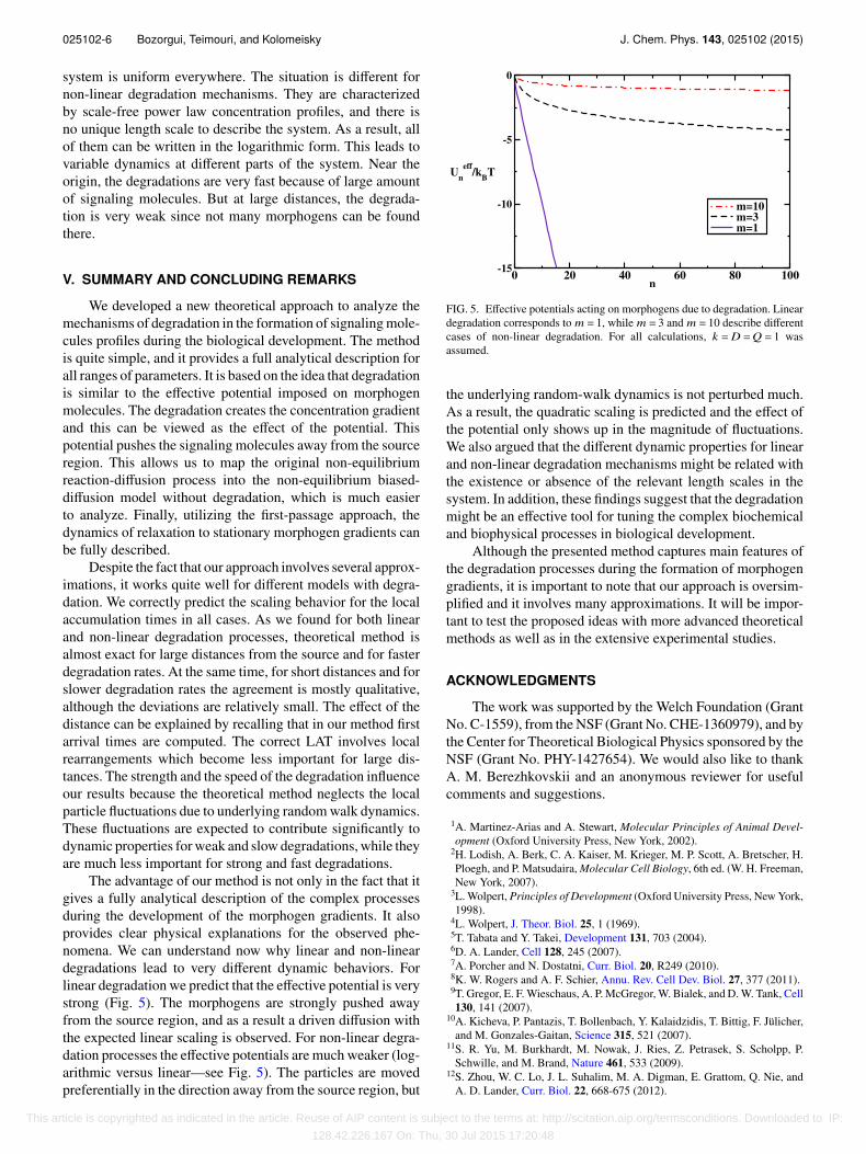
This potential is linear with a slope that depends on diffusionand degradation rates. It is also shown in Fig. 5. Employingthese results in Eqs. (8) and (9), we obtain the followingexpressions for the forward and backward transition rates:

gn = g =2D + kx + 1

, rn+1 = r = x2D + kx + 1

. (12)

Note that these rates are independent of the position and theproduction rate Q.

In the final step, first-passage dynamics can be evaluatedby using known expressions for MFPT,34

τn =

n−1i=0

ij=0

riri−1 · · · r j+1

gigi−1 · · · gj+1gj

=(x + 1)(2D + k)

[x(xn − 1) − n(x − 1)](x − 1)2 . (13)

It can be easily checked that in the special case of no degra-dation in the original system, k = 0, this formula reduces to τn≃ n2/2D at large distances, as expected for a simple unbiasedrandom walk.

It is possible to compare the obtained mean first-passagetimes from Eq. (13) with available analytical expressions forLAT and for MFPT in the original SDD model.22 But it is moreconvenient first to do it for two different dynamic regimes.In the case when the degradation rate is much faster thandiffusion, k ≫ D, it can be shown that x ≃ D/k, which leadsto τn ≃ n/k. This is in excellent agreement with the exactresults for LAT and MFPT for the original SDD model in thislimit,22 tn = τSDD

n ≃ (n + 1)/k. In the opposite limit of very fast

This article is copyrighted as indicated in the article. Reuse of AIP content is subject to the terms at: http://scitation.aip.org/termsconditions. Downloaded to IP:

128.42.226.167 On: Thu, 30 Jul 2015 17:20:48

025102-4 Bozorgui, Teimouri, and Kolomeisky J. Chem. Phys. 143, 025102 (2015)

diffusion (D ≫ k), we have x ≃ 1 −√

k/D and Eq. (13) yields

τn ≃ n/√

kD. (14)

Exact expressions for LAT and MFPT for the original SDDmodel give us22

tn ≃1

2k

1 +

n + 1√

D/k

, τSDD

n ≃ n/2√

Dk . (15)

Thus, for large n our method still correctly reproduces thelinear scaling in the local accumulation times, but the ampli-tude deviates in two times.

The comparison between predicted MFPT for the biased-diffusion model and for LAT of the original SDD model forgeneral sets of parameters is given in Fig. 2. One can see thatour method approximates the dynamics of the formation ofmorphogen gradient reasonably well. The agreement is betterfor larger degradation rates where the effective potentials arestronger. At the same time, for weaker degradation rates thereare deviations, although the qualitative behavior is correctly

FIG. 2. (a) Ratio of the calculated mean first-passage times in the biased-diffusion model and the exact analytical results from the original SDD modelwith linear degradation as a function of the distance from the source. Differentcurves correspond to different values of the degradation and diffusion rates.(b) The same ratio as a function of the ratio of the degradation rate overdiffusion. Distance from the source is set to n = 104, which exceeds the decaylengths for all values of the degradation rates.

captured. This is a remarkable result given how simple is thetheory and that it involves several weak approximations. Thisalso suggests that the method can be reliably applied to morecomplex systems with non-linear degradation.

IV. NON-LINEAR DEGRADATION

Here, we apply our method for systems where the forma-tion of signaling molecules profiles is accompanied by thenon-linear degradation processes with the corresponding rateskn = kPm−1

n for m = 2,3, . . .. To evaluate the effective potentialwe need to estimate the stationary-state concentration profiles.However, it is not possible to calculate them analytically forgeneral non-linear discrete SDD models. But we can use thefact that in the continuum limit (D ≫ kn) original master equa-tions (1) and (2) can be written as the corresponding non-linearreaction-diffusion equations,

∂P(n, t)∂t

= D∂2P(n, t)

∂n2 − kPm(n, t), (16)

with the boundary condition at the origin

D∂P∂n

|n=0 = −Q. (17)

These equations can be solved in the steady-state limit, produc-ing

P(s)n ≃

1

(1 + n/λ) 2m−1

, (18)

where the parameter λ is given by

λ =1

m − 1

(2D)m(m + 1)kQm−1

1m+1

. (19)

It can be shown that the continuum P(s)n describes also quite

well the stationary-state behavior of the general non-lineardiscrete SDD models at large distances from the source. Thisallows us to approximate the effective potentials for non-lineardegradation as

Ueffn

kBT≃ − 2

m − 1ln(1 + n/λ). (20)

This potential is logarithmic, and the degree of non-linearitydetermines its magnitude as illustrated in Fig. 5. It is importantto note here that these potentials are always weaker than thepotential for the linear degradation: see Fig. 5.

Now using Eqs. (8) and (9) one can obtain the expressionsfor transition rates in the biased-diffusion model,

gn = D

P(s)n

P(s)n+1

0.5

, rn+1 = D

P(s)n

P(s)n+1

−0.5

. (21)

In the final step, again utilizing the analytical frameworkfor the first-passage processes,34 we derive the explicit expres-sions for the mean first-passage times that approximate theformation of the morphogen gradients with nonlineardegradation,

This article is copyrighted as indicated in the article. Reuse of AIP content is subject to the terms at: http://scitation.aip.org/termsconditions. Downloaded to IP:

128.42.226.167 On: Thu, 30 Jul 2015 17:20:48

025102-5 Bozorgui, Teimouri, and Kolomeisky J. Chem. Phys. 143, 025102 (2015)

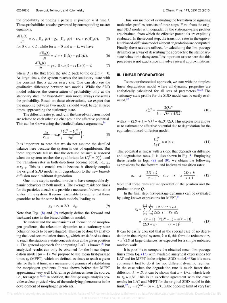
FIG. 3. Theoretically calculated mean first passage times as a function of the distance from the source for different degrees of non-linearity and for differentvalues of the degradation rates: (a) m = 2; (b) m = 10.

τn =

n−1i=0

ij=0

riri−1 · · · r j+1

gigi−1 · · · gj+1gj

=1D

n−1j=0

[ j( j + 1)] 11−m

jl=0

l2

m−1 . (22)

It can be shown that this expression asymptotically at largedistances approaches to

τn ≈(m − 1)(m + 1)

n2

2D. (23)

This is an important result since it predicts a quadratic scalingfor all non-linear degradation mechanisms with m > 1. Fur-thermore, as expected for very large m, which correspondseffectively to the case without degradation, this formula re-duces to a known unbiased random-walk dependence.

Our theoretical estimates for the relaxation dynamics inthe establishment of the morphogen gradients for variousmodels with non-linear degradation are presented in Fig. 3.One can clearly see that the predicted local accumulation timesapproach the quadratic scaling for large n for all possibleranges of diffusion and degradation rates. The approach isfaster for larger m. The scaling is independent of the degra-dation mechanisms, and only the amplitude is determined bythe degree of the non-linearity m.

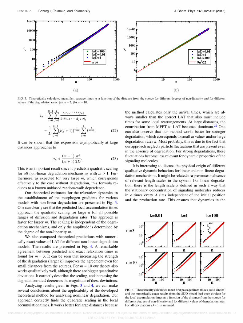
We also compared theoretical predictions with numeri-cally exact values of LAT for different non-linear degradationmodels. The results are presented in Fig. 4. A remarkableagreement between predicted and exact relaxation times isfound for m = 3. It can be seen that increasing the strengthof the degradation (larger k) improves the agreement even forsmall distances from the sources. For m = 10 our theory alsoworks qualitatively well, although there are bigger quantitativedeviations. It correctly describes the scaling, and increasing thedegradation rate k decreases the magnitude of these deviations.

Analyzing results given in Figs. 3 and 4, we can makeseveral conclusions about the applicability of the developedtheoretical method for analyzing nonlinear degradation. Ourapproach correctly finds the quadratic scaling in the localaccumulation times. It works better for large distances because

the method calculates only the arrival times, which are al-ways smaller than the correct LAT that also must includetimes for some local rearrangements. At large distances, thecontribution from MFPT to LAT becomes dominant.22 Onecan also observe that our method works better for strongerdegradation, which corresponds to small m values and/or largedegradation rates k. Most probably, this is due to the fact thatour approach neglects particle fluctuations that are present evenin the absence of degradation. For strong degradations, thesefluctuations become less relevant for dynamic properties of thesignaling molecules.

It is interesting to discuss the physical origin of differentqualitative dynamic behaviors for linear and non-linear degra-dation mechanisms. It might be related to a presence or absenceof relevant length scales in the system. For linear degrada-tion, there is the length scale λ defined in such a way thatthe stationary concentration of signaling molecules reducesin e times every λ sites independent of the initial positionand the production rate. This ensures that dynamics in the

FIG. 4. Theoretically calculated mean first passage times (black solid circles)and the numerically exact results from the SDD model (red open circles) forthe local accumulation times as a function of the distance from the source fordifferent degrees of non-linearity and for different values of degradation rates.For all calculations D = 1 is assumed.

This article is copyrighted as indicated in the article. Reuse of AIP content is subject to the terms at: http://scitation.aip.org/termsconditions. Downloaded to IP:

128.42.226.167 On: Thu, 30 Jul 2015 17:20:48

025102-6 Bozorgui, Teimouri, and Kolomeisky J. Chem. Phys. 143, 025102 (2015)

system is uniform everywhere. The situation is different fornon-linear degradation mechanisms. They are characterizedby scale-free power law concentration profiles, and there isno unique length scale to describe the system. As a result, allof them can be written in the logarithmic form. This leads tovariable dynamics at different parts of the system. Near theorigin, the degradations are very fast because of large amountof signaling molecules. But at large distances, the degrada-tion is very weak since not many morphogens can be foundthere.

V. SUMMARY AND CONCLUDING REMARKS

We developed a new theoretical approach to analyze themechanisms of degradation in the formation of signaling mole-cules profiles during the biological development. The methodis quite simple, and it provides a full analytical description forall ranges of parameters. It is based on the idea that degradationis similar to the effective potential imposed on morphogenmolecules. The degradation creates the concentration gradientand this can be viewed as the effect of the potential. Thispotential pushes the signaling molecules away from the sourceregion. This allows us to map the original non-equilibriumreaction-diffusion process into the non-equilibrium biased-diffusion model without degradation, which is much easierto analyze. Finally, utilizing the first-passage approach, thedynamics of relaxation to stationary morphogen gradients canbe fully described.

Despite the fact that our approach involves several approx-imations, it works quite well for different models with degra-dation. We correctly predict the scaling behavior for the localaccumulation times in all cases. As we found for both linearand non-linear degradation processes, theoretical method isalmost exact for large distances from the source and for fasterdegradation rates. At the same time, for short distances and forslower degradation rates the agreement is mostly qualitative,although the deviations are relatively small. The effect of thedistance can be explained by recalling that in our method firstarrival times are computed. The correct LAT involves localrearrangements which become less important for large dis-tances. The strength and the speed of the degradation influenceour results because the theoretical method neglects the localparticle fluctuations due to underlying random walk dynamics.These fluctuations are expected to contribute significantly todynamic properties for weak and slow degradations, while theyare much less important for strong and fast degradations.

The advantage of our method is not only in the fact that itgives a fully analytical description of the complex processesduring the development of the morphogen gradients. It alsoprovides clear physical explanations for the observed phe-nomena. We can understand now why linear and non-lineardegradations lead to very different dynamic behaviors. Forlinear degradation we predict that the effective potential is verystrong (Fig. 5). The morphogens are strongly pushed awayfrom the source region, and as a result a driven diffusion withthe expected linear scaling is observed. For non-linear degra-dation processes the effective potentials are much weaker (log-arithmic versus linear—see Fig. 5). The particles are movedpreferentially in the direction away from the source region, but

FIG. 5. Effective potentials acting on morphogens due to degradation. Lineardegradation corresponds to m = 1, while m = 3 and m = 10 describe differentcases of non-linear degradation. For all calculations, k =D =Q = 1 wasassumed.

the underlying random-walk dynamics is not perturbed much.As a result, the quadratic scaling is predicted and the effect ofthe potential only shows up in the magnitude of fluctuations.We also argued that the different dynamic properties for linearand non-linear degradation mechanisms might be related withthe existence or absence of the relevant length scales in thesystem. In addition, these findings suggest that the degradationmight be an effective tool for tuning the complex biochemicaland biophysical processes in biological development.

Although the presented method captures main features ofthe degradation processes during the formation of morphogengradients, it is important to note that our approach is oversim-plified and it involves many approximations. It will be impor-tant to test the proposed ideas with more advanced theoreticalmethods as well as in the extensive experimental studies.

ACKNOWLEDGMENTS

The work was supported by the Welch Foundation (GrantNo. C-1559), from the NSF (Grant No. CHE-1360979), and bythe Center for Theoretical Biological Physics sponsored by theNSF (Grant No. PHY-1427654). We would also like to thankA. M. Berezhkovskii and an anonymous reviewer for usefulcomments and suggestions.

1A. Martinez-Arias and A. Stewart, Molecular Principles of Animal Devel-opment (Oxford University Press, New York, 2002).

2H. Lodish, A. Berk, C. A. Kaiser, M. Krieger, M. P. Scott, A. Bretscher, H.Ploegh, and P. Matsudaira, Molecular Cell Biology, 6th ed. (W. H. Freeman,New York, 2007).

3L. Wolpert, Principles of Development (Oxford University Press, New York,1998).

4L. Wolpert, J. Theor. Biol. 25, 1 (1969).5T. Tabata and Y. Takei, Development 131, 703 (2004).6D. A. Lander, Cell 128, 245 (2007).7A. Porcher and N. Dostatni, Curr. Biol. 20, R249 (2010).8K. W. Rogers and A. F. Schier, Annu. Rev. Cell Dev. Biol. 27, 377 (2011).9T. Gregor, E. F. Wieschaus, A. P. McGregor, W. Bialek, and D. W. Tank, Cell130, 141 (2007).

10A. Kicheva, P. Pantazis, T. Bollenbach, Y. Kalaidzidis, T. Bittig, F. Jülicher,and M. Gonzales-Gaitan, Science 315, 521 (2007).

11S. R. Yu, M. Burkhardt, M. Nowak, J. Ries, Z. Petrasek, S. Scholpp, P.Schwille, and M. Brand, Nature 461, 533 (2009).

12S. Zhou, W. C. Lo, J. L. Suhalim, M. A. Digman, E. Grattom, Q. Nie, andA. D. Lander, Curr. Biol. 22, 668-675 (2012).

This article is copyrighted as indicated in the article. Reuse of AIP content is subject to the terms at: http://scitation.aip.org/termsconditions. Downloaded to IP:

128.42.226.167 On: Thu, 30 Jul 2015 17:20:48

025102-7 Bozorgui, Teimouri, and Kolomeisky J. Chem. Phys. 143, 025102 (2015)

13M. Kerszberg and L. Wolpert, J. Theor. Biol. 191, 103 (1998).14E. V. Entchev, A. Schwabedissen, and M. Gonzales-Gaitan, Cell 103, 981

(2000).15P. Müller, K. W. Rogers, B. M. Jordan, J. S. Lee, D. Robson, S. Ramanathan,

and A. F. Schier, Science 336, 721 (2012).16J. A. Drocco, O. Grimm, D. W. Tank, and E. Wieschaus, Biophys. J. 101,

1807 (2011).17A. Spirov, K. Fahmy, M. Schneider, E. Frei, and M. Noll, Development 136,

605 (2009).18S. C. Little, G. Tkacik, T. B. Kneeland, E. Wieschaus, and T. Gregor, PLoS

Biol. 9, e1000596 (2011).19S. Fedotov and S. Falconer, Phys. Rev. E 89, 012107 (2014).20A. M. Berezhkovskii, C. Sample, and S. Y. Shvartsman, Biophys. J. 99, L59

(2010).21P. V. Gordon, C. B. Muratov, and S. Y. Shvartsman, J. Chem. Phys. 138,

104121 (2013).22A. B. Kolomeisky, J. Phys. Chem. Lett. 2, 1502 (2011).

23B. Houchmandzadeh, E. Wieschaus, and S. Leibler, Nature 415, 798 (2002).24J. L. England and J. Cardy, Phys. Rev. Lett. 94, 078101 (2005).25T. B. Kornberg, Biophys. J. 103, 2252 (2012).26A. M. Turing, Philos. Trans. R. Soc. London 237, 37 (1952).27J. A. Drocco, E. Wieschaus, and D. W. Tank, Phys. Biol. 9, 055004 (2012).28O. Grimm, M. Coppy, and E. Wieschaus, Development 137, 2253 (2009).29H. Teimouri and A. B. Kolomeisky, J. Chem. Phys. 140, 085102 (2014).30P. V. Gordon, C. Sample, A. M. Berezhkovskii, C. B. Muratov, and S. Y.

Shvartsman, Proc. Natl. Acad. Sci. U. S. A. 108, 6157 (2011).31A. Eldar, D. Rosin, B.-Z. Shilo, and N. Barkai, Dev. Cell 5, 635 (2003).32Y. Chen and G. Struhl, Cell 87, 553 (1996).33J. P. Incardona, J. H. Lee, C. P. Robertson, K. Enga, R. P. Kapur, and H.

Roelink, Proc. Natl. Acad. Sci. U. S. A. 97, 12044 (2000).34N. G. Van Kampen, Stochastic Processes in Physics and Chemistry (Elsevier

Science B.V., The Netherlands, 2001).35A. M. Berezhkovskii and S. Y. Shvartsman, J. Chem. Phys. 135, 154115

(2011).

This article is copyrighted as indicated in the article. Reuse of AIP content is subject to the terms at: http://scitation.aip.org/termsconditions. Downloaded to IP:

128.42.226.167 On: Thu, 30 Jul 2015 17:20:48