The AI Economist:Improving Equality and Productivity with AI-Driven Tax

Policies

Stephan Zheng*,1, Alexander Trott*,1, Sunil Srinivasa1, Nikhil Naik1, Melvin Gruesbeck1,David C. Parkes1,2, and Richard Socher1

1Salesforce Research2Harvard University

April 28, 2020Abstract

Tackling real-world socio-economic challenges requires designing and testing economic policies. How-ever, this is hard in practice, due to a lack of appropriate (micro-level) economic data and limited opportunityto experiment. In this work, we train social planners that discover tax policies in dynamic economies thatcan effectively trade-off economic equality and productivity. We propose a two-level deep reinforcementlearning approach to learn dynamic tax policies, based on economic simulations in which both agents and agovernment learn and adapt. Our data-driven approach does not make use of economic modeling assump-tions, and learns from observational data alone. We make four main contributions. First, we present aneconomic simulation environment that features competitive pressures and market dynamics. We validate thesimulation by showing that baseline tax systems perform in a way that is consistent with economic theory,including in regard to learned agent behaviors and specializations. Second, we show that AI-driven taxpolicies improve the trade-off between equality and productivity by 16% over baseline policies, including theprominent Saez tax framework. Third, we showcase several emergent features: AI-driven tax policies arequalitatively different from baselines, setting a higher top tax rate and higher net subsidies for low incomes.Moreover, AI-driven tax policies perform strongly in the face of emergent tax-gaming strategies learned byAI agents. Lastly, AI-driven tax policies are also effective when used in experiments with human participants.In experiments conducted on MTurk, an AI tax policy provides an equality-productivity trade-off that issimilar to that provided by the Saez framework along with higher inverse-income weighted social welfare.

* indicates significant contribution. R.S. and S.Z. conceived and directed the project; S.Z., A.T., N.N., and D.P. developed thetheoretical framework; A.T. and S.Z. developed the economic simulator; A.T. and S.Z. implemented the reinforcement learningplatform and performed experiments with AI agents; A.T., S.Z., and D.P. processed and analyzed experiments with AI agents; S.Z.implemented and performed the experiments with human participants; M.G., N.N., and S.Z. designed the interface for humanparticipants; S.S. and S.Z. processed the results with human participants; S.Z., A.T., S.S., N.N., and D.P. interpreted the results withhuman participants; A.T., M.G., S.S., and S.Z. designed the figures and visualizations; S.Z., A.T., N.N., and D.P. drafted the manuscript;Kathy Baxter drafted the ethical review; R.S. planned and advised the work, and analyzed all results; all authors discussed the resultsand commented on the manuscript. We thank Kathy Baxter, Lofred Madzou, Simon Chesterman, Rob Reich, Mia de Kuijper, ScottKominers, Gabriel Kriendler, Stefanie Stantcheva, and Thomas Piketty for valuable discussions. This research was not conductedwith any corporate or commercial applications in mind. Correspondence to: stephan.zheng@salesforce.com.

1

arX

iv:2

004.

1333

2v1

[ec

on.G

N]

28

Apr

202

0

1 IntroductionEconomic inequality is accelerating globally and is a key social and economic concern. Many studies haveshown that large income inequality gaps can have significant negative effects, leading for example to diminishedeconomic opportunity [United Nations, 2013] and adverse health effects [Subramanian and Kawachi, 2004].In this light, tax policy provides governments with an important tool to reduce inequality, supporting thepossibility of the redistribution of wealth through government provided services and benefits. And yet, findingthe optimal tax policy is challenging. The basic reason is that while more taxation can improve equality,taxation can also discourage people from working, leading to lower productivity.

The problem of optimally balancing equality and productivity has not been solved for general economicsettings, and even when the policy objectives can be agreed upon. Part of the challenge is that is hard toexperiment with real-world tax policies. In the place of experimentation, economic theory often relies onsimplifying assumptions that are hard to validate, for example about people’s sensitivity to taxes. Tax systemsthat have been proposed range from no taxes at all (“free market”), to progressive and regressive tax systems(reflecting whether the tax rate increases or decreases as income increases), to total redistribution.

In this paper, we introduce “The AI Economist,” a two-level deep reinforcement learning (RL) frameworkto train social planners. The economic actors are adaptive, learning behaviors in the simulated world andincluding in response to tax policy. The planner is also adaptive, learning tax policies that adapt to agentbehaviors and seek to achieve a particular policy objective. Neither economic actors nor the AI Economist haveprior knowledge, whether about the simulated world environment or economic theory. The AI Economistlearns a tax policy based only on observable data and without knowledge of the skill or utility functions ofworkers or prior assumptions about the behavior of workers, and can be used to optimize for any desiredsocial outcome.

The AI Economist learns a tax schedule, analogous to the way in which US federal income taxes aredescribed. Taxes are computed by applying a tax rate to each part of an individual’s income that falls within atax bracket. For simplicity, we fix the intervals that correspond to each of these income brackets and learnthe tax rate for each bracket. The tax schedule learned by the AI Economist is not personalized; each agentfaces the same rates and bracket cutoffs. In a single tax period the tax schedule is determined via a deep neuralnetwork, able to observe all public information about the world, including the position, income, and resourcesheld by agents.

Our approach to economic design is based on the use of simulations, making use of AI agents that learnoptimal behaviors. This use of simulation enables the testing of economic policies at large-scale, and includingthe ability to measure a range of different metrics. In effect, we can compare the performance of millionsof economic designs, making use of economic agents whose behavior is learned in parallel. The simulationframework can also be used to speed up experiments with existing proposals for tax systems, validatingassumptions and offering the ability to test ideas that come from economic theory.

We make the following contributions:

• We introduce a principled economic simulation that features competitive pressures, trade, and resourcescarcity.

• We validate that learned behavior conforms to results known from economic theory, for example agentspecialization.

• We frame the problem of learning optimal taxes in a dynamic economy as a two-level, inner-outerreinforcement learning problem and describe a range of techniques to stabilize training for this two-levelRL problem, including the use of learning curricula and entropy-based regularization.

2

• The AI-driven tax policies make use of different kinds of tax rate schedules than those suggested bybaseline policies, and our experiments demonstrate that the AI-driven tax policy can improve the trade-offbetween equality and productivity by 16% when compared to the prominent Saez tax framework.

• We show that AI agents can learn tax-avoidance behaviors, modulating their incomes across tax periods.The tax schedule generated by the AI Economist performs well despite this kind of strategic behavior.

• Without endorsing the particular tax schedules, we show that a learned policy can also be effectivein experiments with human participants and without additional recalibration. The policy achievesan equality-productivity trade-off that is competitive with the state-of-the-art, together with higherinverse-income weighted social welfare. This provides a preliminary suggestion that the AI Economistmethodology could also be applicable to more general, real world settings.

1.1 Related WorkOptimal Taxation. In economics, optimal tax theory is the study of the design of a tax system that maxi-mizes a social welfare function subject to a set of economic constraints, while accounting for the fact thatindividuals respond to taxes and transfers [Mankiw et al., 2009, Diamond and Saez, 2011]. The core challenge inthe design of optimal tax policies is that taxes and transfers can affect incentives to work, creating a trade-offbetween equality and productivity [Mankiw et al., 2009, Diamond and Saez, 2011]. A particular concern is thathigh income may correlate with high skill, leading higher skilled workers to choose to work less.

Ramsey [1927]’s early work tied consumption taxes on a good to a representative consumer’s elasticity ofdemand for the good. The current dominant theoretical framework arose out of a series of papers by Mirrleesand Diamond [Diamond and Mirrlees, 1971a,b, Mirrlees, 1976]. These authors consider a utilitarian socialplanner—aiming to maximize the sum of individual utilities in a society. Saez [2001] builds on the Mirrleesframework to derive optimal non-linear tax rates using models of the elasticity of earnings with respect to taxrates, together with the shape of the income distribution.

Other work has expanded upon the Mirrlees framework to argue for a tax system that tries to achievea broader distributive justice [Piketty and Saez, 2013, Piketty et al., 2014, Saez and Stantcheva, 2016], or a taxsystem in which the payments made by an individual merely match the benefits received [Mankiw et al., 2009,Mankiw, 2010, Mankiw and Weinzierl, 2010].

The Mirrlees model is limited to optimal taxation in a single tax period, without considering dynamics,for example the income histories of individuals in deciding taxes, or events with longer-term effects such aseducation. The new dynamic public finance (NDPF) expands upon these frameworks to consider dynamiceconomies, capturing additional real world effects, for example, allowing for the coordinated taxation ofcapital and labor income [Golosov et al., 2003, Kocherlakota, 2005, Albanesi and Sleet, 2006, Kocherlakota,2010].

Progress in optimal taxation theory has also come through a growing empirical and experimental literature.This includes work that seeks to estimate labor supply elasticity to changes in taxation and redistribution [Gru-ber and Saez, 2002, Chetty, 2012, Goldberg, 2016], and work that seeks to understand the behavioral responseof workers to tax policy through the use of cross-sectional data on taxation, labor supply, and individualincomes [Slemrod, 1996, Goolsbee, 2000, Alesina et al., 2005]. Research in behavioral public finance [McCaf-fery and Slemrod, 2006, Kuziemko et al., 2015, Alesina et al., 2018] makes use of experiments and surveys tounderstand how people respond to different theories of taxation, redistribution, and public spending.

Our work adopts baselines from optimal taxation theory, by comparing the performance of the AIEconomist with tax policies that arise from the Saez framework, in this case, making use of estimated laborelasticities in our simulated economies.

3

Agent-based Modeling. Agent-based modeling (ABM) research [Holland and Miller, 1991, Bonabeau, 2002]creates simulations of agents and institutions that interact through prescribed rules. ABM does not rely onstandard equilibrium models. Rather, it allows for dynamic, nonlinear behavior by agents and institutions,and can adopt behavioral rules that are deduced from human experiments [Arthur, 1991].

The idea is to use ABM to enable policy-makers to simulate an artificial economy under different policyscenarios, and quantitatively explore their consequences [Farmer and Foley, 2009]. ABM has been appliedto study tax compliance [Bloomquist, 2011, Miguel et al., 2012, Subburaj and Rao, 2018], and to derive optimaltaxation policy [Garrido and Mittone, 2013], based on heuristics and simple learning methods. Wider adoptionof ABM has proved challenging due to the complexity of realistically modeling human behavior and theeconomy.

While our motivations are similar to ABM, our framework makes use of deep RL to optimize the behaviorsof economic agents with the effect that we study policy design in the presence of rational agent behavior.

Reinforcement Learning. Our learning approach relates to multi-agent reinforcement learning (MARL). InMARL, agents need to learn together with other learning agents, creating a non-stationary environment [Lau-rent et al., 2011]. This poses a challenge to the standard approach of learning from exploration [Sutton andBarto, 2018a], since agents can easily mistake other agents’ exploration as environment randomness [Claus andBoutilier, 1998]. A particular challenge presented by the AI Economist is that it presents a two-level learningproblem, in which the social planner learns a tax policy simultaneously with agents who learn how to optimizetheir behavior. In effect, agents face a continuously changing reward function. As a consequence, past optimalbehavior might not be optimal at later times, which can present a significant learning challenge.

MARL has been effective in learning emergent cooperation in large-scale experiments on complex envi-ronments [Bansal et al., 2017, Jaderberg et al., 2018, OpenAI, 2018]. Previous MARL algorithms have sought tostabilize multi-agent learning by explicitly modeling missing state or policy information [Lowe et al., 2017,Tacchetti et al., 2018, Shu and Tian, 2018], or assuming some information is shared between agents, includingthe internal or global state or rewards [Sunehag et al., 2017, Foerster et al., 2017, Peysakhovich and Lerer, 2017,Hughes et al., 2018, Letcher et al., 2018, Balduzzi et al., 2018].

In the present paper, we insist on each agent having a policy that only makes use of information that itcan individually observe. To make learning efficient, we allow for weight sharing during training. Learnedagent behaviors remain distinct, as a result of distinct local states, for example, location in the world, skill, andendowment of resources. This presents a hybrid approach, improving learning efficiency without assuminginformation or state sharing between agents.

Optimal taxation can be seen as a form of reward shaping, which has found a role in preventing undesiredsocial outcomes in multi-agent systems, such as unsustainable resource collection in tragedy-of-the-commonsstyle social dilemmas [Leibo et al., 2017]. Reward shaping has also been shown to induce cooperation inspatiotemporal games [Mguni et al., 2019, Hughes et al., 2018, Jaques et al., 2018]. However, these works do notconsider the kinds of economic environments we study here, do not consider the design of tax policies, andmake use of manually-crafted reward shaping.

Machine learning forEconomicDesign. The problemof automatedmechanism designwas first formalizedby Conitzer and Sandholm [2002, 2004], and there are polynomial time algorithms for the design of Bayesianincentive-compatible, optimal auctions [Cai et al., 2012a,b, 2013]. Dütting et al. [2019] were the first to study theuse of deep machine learning for the design of the allocation and payment rules of revenue-optimal auctions.By insisting on incentive-compatible or approximately incentive-compatible designs, their framework canreproduce known optimal designs and also be applied to problems out of reach of current theory. Subsequentwork has also adopted neural networks for the design of optimal auctions in settings with budget-constrainedbidders [Feng et al., 2018], for the design of auctions in settings with payment redistribution [Tacchetti et al.,

4

2019], for single-bidder settings [Shen et al., 2019], as well as for problems of social choice [Golowich et al., 2018].The use of machine learning for the design of auction mechanisms was earlier pioneered by Dütting et al.[2014], who studied the design of payment rules for a given allocation rule. Another line of work explores thesample complexity of the problem of learning an optimal auction, typically focusing on simpler settings [Coleand Roughgarden, 2014, Morgenstern and Roughgarden, 2015, Balcan et al., 2016, Gonczarowski and Weinberg,2018]. Earlier work studied the use of machine learning for the design of voting rules [Procaccia et al., 2009]and for matching and assignment problems [Narasimhan et al., 2016, Narasimhan and Parkes, 2016].

In the aforementioned settings, the agents do not learn how to behave. Rather, the economic policies(typically auctions) are designed such that truthful behavior is optimal for an agent. This avoids the need fortwo-level learning, where agent behaviors are learned at the same time as an economic policy is learned. Anearlier literature did study the co-evolution of agent behaviors and economic designs, but without making useof reinforcement learning and without studying tax polices [Byde, 2003, Phelps et al., 2002, 2010]. Stackelbergequilibria have also been widely studied in other kinds of sequential environments, especially security games.These are two-level problems where the policy of the first-mover (the defender) induces an environment forthe second-mover (the attacker) [Pita et al., 2008, Tambe, 2012]. Recent work has adopted MARL for the studyof security games [Wang et al., 2019, Shah et al., 2019]. Two-stage problems also arise in multi-agent problemswhere the behavior of some agents is optimized in order to improve the overall system behavior [Dimitrakakiset al., 2017, Carroll et al., 2019, Tylkin et al., 2020]. Other work has made use of reinforcement learning to studyresource allocation games such as Blotto [Balduzzi et al., 2019].

Closest in spirit to the present paper, but used for the design of allocation mechanisms rather than fortax policy (for example matching sellers to buyer queries at Taobao and for internet advertising at Baidu),is the work of Tang [2017] and Shen et al. [2020], who make use of RL to improve market design while alsoallowing for agent behavior to respond to new rules. Thompson et al. [2017] have also advanced the idea ofthe “Positronic Economist" (see also Vorobeychik et al. [2012] and Bünz et al. [2018]), which, borrowing fromAsimov’s positronic brain, describes a system that can be used to represent and then automatically analyzethe equilibria that correspond to the rules of economic mechanisms. Parkes and Wellman [2015] have written,generally, about the role of economic design in economies in which transactions are increasingly mediatedthrough AI systems.

1.2 OutlineIn Section 2, we describe our use of economic simulations and the structure of these simulations. We explainthe basic economic drivers and principles that govern the economic AI agents. We then showcase the resultingsocial outcomes, such as equality and productivity, in such worlds. In Section 3, we describe how optimaltaxes can shape socioeconomic outcomes, and the central dilemma of balancing equality and productivity.We introduce our RL approach to learning optimal taxes through interaction with economic simulations.In Section 4, we provide empirical results that validate the effectiveness of the AI Economist in optimizingsocial outcomes. We analyze the qualitative behavior of AI-driven taxes and economic AI agents. In Section 5,we show that the AI Economist is also effective in experiments on Amazon Mechanical Turk (MTurk), withhuman participants earning money. We conclude in Section 6 with a discussion of future directions, andpresent our ethical review in Section 7.

2 Economic Simulations: Learning in Gather-and-Build GamesThis section introduces our framework for studying economic design through simulation with AI agents. Wedescribe the core mechanics of the simulated environment, including the objective that AI agents are trainedto optimize, and we describe the emergent behavior that is typical of economic AI agents in this setting. For

5

ease of exposition, we focus this section on experiments with no taxes applied (“free-market”) in order toillustrate the kinds of social outcomes that taxes may help to correct and some of the challenges faced whendesigning an optimal taxation scheme.

2.1 Notation and PreliminariesIn this work, we use notation that borrows from both the reinforcement learning and the optimal tax theoryliterature, see Table 1.

t timei, j, k agent indicesθ, ϕ model weightss stateo observationa actionr rewardπ policyγ discount factorT state-transition, world dynamicsh hidden state

x endowmentxc coinxs stonexw woodz incomel laboru utilityT taxτ tax-rateπp planner policyswf social welfareω social welfare weightg social marginal welfare weightgini Gini indexeq Equality index

Table 1: Notation. Subscripts are indices. Superscripts are labels.

Formally, we build on the framework of partial-observable multi-agent Markov Games (MGs) [Suttonand Barto, 2018b], defined by the tuple (S, A, r,T, γ, o,I), where S and A are the state and action spaces,respectively, and Iare agent indices. Bold-faced quantities denote vectors, e.g., a = (a1, . . . , aN ), the actionprofile for N agents. MGs proceed in episodes that last H + 1 steps (possibly infinite), covering H transitions.At each time t ∈ [0, H], the world state is denoted st . Each agent i = 1, . . . ,N receives an observation oi,t ,executes an action ai,t and receives a reward ri,t . The environment transitions to the next state st+1, accordingto the transition distribution T(st+1 |st, at). Agent-specific observations oi,t describe the portion of the state stthat agent i is able to observe.

Each agent learns a policy πi(ai,t |oi,t, hi,t; θi

)that maximizes its γ-discounted expected return, where the

policy is conditioned on the history of past observations bymaintaining a hidden state hi,t , andwhere θi parame-terizes the policy of agent i. Let π = (π1, . . . , πN ) denote the joint policy and π−i = (π1, . . . , πi−1, πi+1, . . . , πN )denote the policy without agent i. Through reinforcement learning, agent i seeks a policy to solve

maxθi

Eai∼πi,a−i∼π−i,s′∼T

[∑tγ tri,t

], (1)

for discount factor γ ∈ (0, 1). Equation 1 describes an agent i that maximizes its expected reward, whichdepends on the behavioral policies π−i of the other agents and the environment transition dynamics T. Thisis a policy that best responds to the policies of other agents, given the dynamics of the simulated environmentand an agent’s observations.

6

Figure 1: The Gather-and-Build game. Agents move around, collect resources (wood and stone) and buildhouses. Agents cannot move through each others’ houses, or move through water. Agents can trade resources.

For data efficiency, all agents share the same parameters during training, denoted θ, but condition theirpolicy πi (ai |oi, hi; θ) on agent-specific observations oi and hidden-state hi. In effect, if one agent learns a usefulnew behavior for some part of the state space then this becomes available to another agent. At the same time,agent behaviors remain heterogeneous because they have different observations and hidden states.

2.2 Environment Rules and DynamicsOverview. We introduce the Gather-and-Build game, a two-dimensional grid-world in which agents canmove to collect resources, earn coins by using the resources of stone and wood to build houses, and tradewith other agents to exchange resources for coins. Stone and wood stochastically spawn on special resourceregeneration tiles. Agents can move around the environment to gather these resources from populatedresource tiles that remain empty after harvesting until some new resources spawn.

Agents can choose to use one unit of wood and one unit of stone to construct a house, and this places ahouse tile at the agent’s current location and earns the agent some number of coins. The number of coinsearned per house depends on the skill of an agent, and skill is different across agents. In addition, agentsstart at different initial locations in the world. These heterogeneities are the main driver of both economicinequality and specialization in our environment.

Agents can also trade resources, by submitting the number of coins they are willing to accept (an ask) orare willing to pay (a bid), respectively, to an open market, for each of wood and stone. We provide a detaileddescription of the environment and its underlying dynamics in the appendix (Section A).

Labor and Skill. Over the course of an episode (a single play out of the environment), agents accumulatelabor cost, which reflects the amount of effort associated with the actions taken by the agent. Each type ofaction (moving, gathering, trading, and building) is associated with a specific labor cost. Each time an agentperforms one of these actions, its accumulated labor is incremented by the action’s associated labor cost.As described below (Section 2.3), agent rewards depend positively on accumulated coin and negatively onaccumulated labor. The labor costs associated with each action type are calibrated so that agents need to bestrategic in how they choose to earn income, and all agents experience the same labor costs.

7

Following taxation theory, we allow agents in the environment to vary by skill, which describes howmuchincome an agent is able to earn per unit of labor. We capture this by providing, separately for each agent, (1) amultiplier on the default number of coins earned from building a house, and (2) the probability of gainingbonus resources when harvesting. The coin payoff for a house depends linearly on skill. An agent receives aminimum of 10 coin per house built.

A building skill of 1 (the minimum value) means the agent earns this minimum payoff and a building skill of2.5 means the agent receives 25 coin per house. The maximum skill value is 3. An agent’s collection skill is equalto the average number of resources it receives each time it steps on a populated stone or wood resource tile.As an example, for an agent with a collection skill of 1.2, it will always receive at least 1 resource from steppingon a populated tile and there is a 20% chance it will also receive a bonus unit of the collected resource. Theminimum collection skill is 1 and the maximum is 2, ranging from never receiving bonus resource units toalways receiving them.

We conceptualize the coins that are generated when building a house as coming from a part of the widereconomy that our simulation does not directly model. An agent’s building skill— the coin the agent receivesfrom building —reflects the value that this external market places on a particular agent’s houses. The totalquantity of coins generated by the simulated agents during an episode reflects the value created by theircollective labor.

Environment Scenario. All experiments were carried out using the specific world map shown in Figure 1,which has four quadrants, mostly separated by water from each other (this blocks movement), and withspatially clustered resources. We focus on games with four agents, and apply a fixed set of building skills,chosen as the means of the quartiles of a clipped Pareto distribution with exponent a = 4 and scale m = 1.Skills and starting locations are randomly assigned to agents. These building skills correspond to payoffs of11.3, 13.3, 16.5, and 22.2 coins per house. In all experiments, we used episodes of length H = 1000 time steps.

2.3 Using Machine Learning to Optimize Agent BehaviorTo ground our simulation in economic theory, we model the reward that the agents learn to optimize as autility function. Recall that xi,t denotes the endowment of resources (stone and wood) and coin owned by anagent at time t. At time t, the utility experienced by an agent i is a function of the number of coins that it hasaccumulated xci,t , and the total labor that it has exerted li,t . In particular, we adopt a utility function that isconcave and increasing in money, and linearly decreasing in labor:

ui(xi,t, li,t) = crra(xci,t

)− li,t, crra (z) = z1−η − 1

1 − η , η > 0. (2)

Here, li,t is the cumulative labor associated with the actions taken by the agent up to time t, and the concaveisoelastic utility crramodels diminishing marginal utility over money [Debreu, 1968]. Parameter η controlsthe degree of nonlinearity: higher η represents larger deviations from linear behavior. We assume that allagents share the same form of utility function. This utility function is visualized in Figure 2 for a simple settingwithout trading and where there is no labor cost associated with moving or gathering resources.

Rational economic agents optimize their total discounted utility over time, with

∀i : maxπi

Eai∼πi,a−i∼π−i,s′∼T

H∑t=1

γ t(ui(xi,t, li,t) − ui(xi,t−1, li,t−1)

)︸ ︷︷ ︸= ri,t

+ui(xi,0, li,0)

. (3)

8

Figure 2: Agent utility, as defined in Equation 2, in a simplified setting where utility only depends on thenumber of houses built, for four agents with different skills n0 < . . . < n3. For clarity of this visualization,each agent is assumed to receive a fixed income per house, which increases with skill, as described in Section2.2. For each house built, each agent is also assumed to have exerted a fixed amount of labor. Hence, in thissimple example, agent utility only depends on the number of houses built. Each agent experiences a lawof diminishing returns (marginal utility decreases as income grows). As agent skill increases, the point ofmaximal utility is reached at a higher number of houses built.

In the paradigm of RL, this is achieved by defining the instantaneous reward ri,t for agent i as the changein utility of agent i at time t.

Equation 3 describes a multi-agent optimization problem, when the agents are simultaneously optimizingtheir behavior, since the utility for agent i depends on the behaviors of other agents (for example, theirgathering, building and trading actions). For instance, another agent might block an agent’s access to resources,which would impact how many houses the agent can build in the future and hence its future utility.

In general, such optimization problems are described as partially-observable multi-agent Markov games,and optimal solutions correspond to refinements of Nash equilibria. A set of policies form a Nash equilibriumas long as no agent wants to unilaterally deviate from its own policy. Refinements such as subgame-perfectequilibria also require rational, off-equilibrium behavior. Although computing equilibria for complex envi-ronments such as this remains out-of-reach, we will see that RL can nevertheless be used to achieve sensible,emergent behaviors (and behaviors that also drive good tax policy, when coupled with the use of the AIEconomist).

Deep RL agents. We make use of a deep neural network to model agent policies,

ai,t ∼ π(oworldi,t , oagenti,t , o

marketi,t , otaxi,t , hi,t−1; θ). (4)

The output of this policy network includes a probability distribution over actions, with ai,t sampled fromthis distribution. Not represented in the notation, the policy network also generates an updated hidden statehi,t . The inputs to the network include the agent-specific hidden state and agent-specific observations, whichare decomposed as follows:

9

Endowment

Endowment

<

<

Market Behavior

Tax Rates

<<

*

*

*

<*

<

<<

<< Agent Observations

Planner Observations

Agent Model

Agent Actions (50)

MLPCNN LSTM MLP

Move

Trade

Build

Private State

SkillLabor

SkillLabor

<

<

Planner Model

Planner Actions (7x22)

MLPCNN LSTM MLP

Set Bracket 1

...

Set Bracket 7

Semi-Private StatePublic State

Public Map

Figure 3: Schematic overview of the general network architecture used in our work. Spatial observationsare processed by a stack of two convolutional layers (CNN) and flattened into a fixed-length feature vector.This feature vector is concatenated with the remaining observation inputs and the result is processed by astack of two fully connected layers (MLP). The output is then used to update the hidden state of an LSTM andaction logits are computed via a linear projection of the updated hidden state. Finally, the network computesa softmax probability layer for each action head. For the agent policy, there is a single action space and actionhead. For the tax policy, there is a separate action space and action head for each tax rate the tax policycontrols (described below).

• oworldi,t : spatial observations from the nearby world.

• oagenti,t : the public agent state (such as resource and coin endowments), as well as the private agent state(such as skill values and labor performed).

• omarketi,t : the full market state, including available offers to buy/sell resources.

• otaxi,t : the tax rates in effect.2

Section A of the appendix provides exact details of the information available in the agents’ observations.The learned hidden state hi,t is used to encode the history of past observations. Figure 3 depicts the generalnetwork architecture used here.

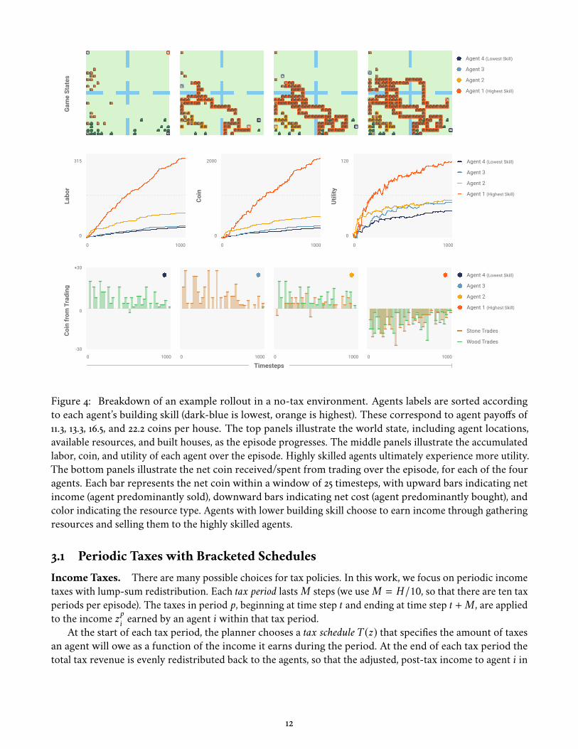
Emergent Behavior of AI Agents. Figure 4 provides a breakdown of an example rollout of play by AIagents across a single episode, once training has proceeded for a large number of episodes. Each agent

2We include tax information even for the free-market, when all tax rates are zero. This ensures that the structure of theobservations is the same for all taxation schemes.

10

has a unique color. Agents are ordered from low to high skill as dark-blue, light-blue, yellow, and orange,corresponding to payoffs of 11.3, 13.3, 16.5, and 22.2 coins per house, respectively.

This rollout reveals an interesting specialization of effort. The dark- and light-blue agents focus entirelyon collecting wood and stone (respectively), the orange agent focuses almost entirely on building houses, andthe yellow agent builds several houses early on before switching to collecting and selling.

This pattern of behavior and division of labor is typical of agents trained in this simulated environment,and stems from the different incomes each agent can earn per house it builds, as well as the agents’ initiallocations in the world. In particular, the low skilled dark- and light-blue agents learn to shift their strategiesentirely away from building houses. These agents earn their income by selling resources to the higher skilledagents, who choose to earn income through building (Figure 4, middle). The yellow agent earns enoughincome from building to do so early on, making use of the nearby resources, but then switches strategies.

This specialization is a consequence of agents learning to maximize their own individual objectives. We donot impose these roles or behaviors directly. Rather, this specialization arises as a result of differently skilledworkers learning to balance their income and effort. This emergent behavior helps to validate the frameworkas an economic simulation, by reproducing a standard feature of real world economies, that of specialization.Standard economic intuition states that agents should specialize in whichever means of production allowsthem to most efficiently convert their labor to income, and this is consistent with the behaviors that the AIagents discover.

Even with specialization, the agents’ incomes can vary considerably. While a free-market economymaximizes productivity, it provides no guarantee on income equality. This is evident in the highly unequalincomes experienced by the AI agents.

3 Machine Learning for Optimal Tax PoliciesWe now introduce a social plannerwho uses economic policy to improve social outcomes, in particular taxationtogether with redistribution. The challenge is that taxation can reduce productivity. Workers may choose toforgo labor as a result of paying tax on income, and thus gaining less utility for labor effort. This may have aparticularly strong effect on the higher skilled and thus more productive workers. Thus, there is a trade-offbetween equality and productivity: the same interventions that allow wealth to be redistributed also resultin there being less wealth to redistribute in the first place. As a result of this coupling between taxation andlabor, determining an optimal tax policy poses a difficult, constrained optimization problem.

A conceptual view of the trade-off between productivity and equality for different tax policies is illustratedin Figure 5. The spectrum of tax policies has two extremes: the free market, which only considers productivityand does not raise any taxes; and pure redistribution, which divides all incomes equally amongst all workersand thus achieves equality but at the potential cost of a large drop in productivity. Here, the notion ofoptimality implies that a tax policy realizes a trade-off between equality and productivity along the Paretoboundary linking these two extremes. The optimal tax literature has proposed several solutions, including thetax formula proposed by Saez [2001] (shown here, together with the AI Economist, with purely illustrativetradeoffs). But the results from optimal tax policy are limited to simple economic models, and require varioussimplifying assumptions, for example about the effect of higher taxes on labor choices.

The remainder of this section describes our approach for studying optimal taxation. We describe thekind of tax policy learned by the AI Economist, define the types of social objectives that can be adopted, anddescribe how we use reinforcement learning to jointly optimize agent behavior as well as the tax policy usedin the economy.

11

10000

Agent 4 (Lowest Skill)

Agent 3

Agent 2

Agent 1 (Highest Skill)

10000 10000 10000

Coin

from

Tra

ding

-30

0

Stone Trades

Wood Trades

+30

Timesteps

Labo

r

315

0

10000

Coin

2000

0

10000

Utili

ty

120

0

10000

Agent 2

Agent 3

Agent 4 (Lowest Skill)

Agent 1 (Highest Skill)

Agent 2

Agent 3

Agent 1 (Highest Skill)

Agent 4 (Lowest Skill)

Gam

e St

ates

Figure 4: Breakdown of an example rollout in a no-tax environment. Agents labels are sorted accordingto each agent’s building skill (dark-blue is lowest, orange is highest). These correspond to agent payoffs of11.3, 13.3, 16.5, and 22.2 coins per house. The top panels illustrate the world state, including agent locations,available resources, and built houses, as the episode progresses. The middle panels illustrate the accumulatedlabor, coin, and utility of each agent over the episode. Highly skilled agents ultimately experience more utility.The bottom panels illustrate the net coin received/spent from trading over the episode, for each of the fouragents. Each bar represents the net coin within a window of 25 timesteps, with upward bars indicating netincome (agent predominantly sold), downward bars indicating net cost (agent predominantly bought), andcolor indicating the resource type. Agents with lower building skill choose to earn income through gatheringresources and selling them to the highly skilled agents.

3.1 Periodic Taxes with Bracketed SchedulesIncome Taxes. There are many possible choices for tax policies. In this work, we focus on periodic incometaxes with lump-sum redistribution. Each tax period lastsM steps (we useM = H/10, so that there are ten taxperiods per episode). The taxes in period p, beginning at time step t and ending at time step t +M, are appliedto the income zpi earned by an agent i within that tax period.

At the start of each tax period, the planner chooses a tax schedule T(z) that specifies the amount of taxesan agent will owe as a function of the income it earns during the period. At the end of each tax period thetotal tax revenue is evenly redistributed back to the agents, so that the adjusted, post-tax income to agent i in

12

Wealth Distribution by Tax Model

Free Market AI EconomistSaez FormulaUS Federal

Top Agent Typical Agent

0%

LowProductivity

Equa

lity

High

100%

AI Economist

Saez Formula

Free Market

US FederalPareto Boundary

Equality-Productivity Trade-off

Figure 5: A conceptual view of how taxes can impact social outcomes. Left: Taxes can improve equality bytransferring wealth. However, taxes can also decrease productivity, because they can discourage work. TheAI Economist seeks a tax policy that optimizes this trade-off. The Pareto boundary is the set of maximaltrade-offs. Right: Taxes impact productivity (total income, represented by the area of the big squares), andequality (the relative difference in sizes of the smaller squares). The AI Economist achieves the best trade-off(measured in equality times productivity).

period p is given by

zpi = zpi − T(z

pi ) +

1N

N∑j=1

T(zpj ). (5)

At the end of an episode, each agent’s coin endowment is the sum of its post-tax incomes in each period:xci,H =

∑p z

pi .

Bracketed Tax Schedules. To allow comparison across different schemes, we adopt income brackets fordescribing a tax schedule, imitating the US federal taxation scheme. A bracketed schedule defines a set ofcut-off income levels mb, where b = 0, . . . B, for B income brackets. The edges of bracket b are [mb,mb+1], and,by definition, m0 = 0 and mB = ∞. The social planner sets the tax schedule T(z) by choosing the marginal taxrate τ ∈ [0, 1]B to be applied within each bracket.

Given this, the total tax payment T(z) for an agent earning z in a tax period is determined by taking thesum of the amount of income within each bracket [mb,mb+1] times that bracket’s marginal rate τb:

T(z) =B−1∑b=0

τb · ((mb+1 − mb) 1[z > mb+1] + (z − mb) 1[mb < z ≤ mb+1]) , (6)

where 1[z > mb+1] ∈ {0, 1} is an indicator function for whether z saturates bracket b and 1[mb < z ≤mb+1] ∈ {0, 1} is an indicator function for whether z falls within bracket b.

3.2 Optimal TaxationSocialWelfare Functions. The objective of optimal tax theory is described through a social welfare functionswf. Social welfare can be expressed in many ways. One approach considers the trade-off between incomeequality and productivity. For this, the equality in an economy at some point in time can be defined as thecomplement of the normalized Gini index on the distribution on wealth, this wealth defined as the cumulativenumber of coins owned by an agent after taxation and redistribution.

13

For an agent population with monetary endowments xc = (xc1, . . . , xcN ), we define equality eq(xc) as:

eq(xc) = 1 − gini(xc) NN − 1, 0 ≤ eq(xc) ≤ 1, (7)

where the Gini index is defined as,

gini(xc) =∑Ni=1

∑Nj=1 |xci − x

cj |

2N∑Ni=1 x

ci

, 0 ≤ gini(xc) ≤ N − 1N. (8)

Given this, eq = 1 implies perfect equality (all endowments of money are identical), while eq = 0meansperfect inequality (one agent owns all money). The productivity in an economy at some point in time is definedas the sum of all wealth over all agents:

prod(xc) =N∑i=1

xci . (9)

We write eqt(xct ) and prodt(xct ) to denote the equality and productivity, respectively, based on the cumulativeendowment xct up to time t.

The primary social welfare function that we consider in this work optimizes a trade-off between equalityand productivity, defined as the product of equality and productivity:

swft(xct ) = eqt(xct ) · prodt(xct ). (10)

Another family of social welfare functions, and one that receives attention in the optimal taxation theory,is the family of linear-weighted sums of agent utilities, defined for weights ωi ≥ 0:

swft(xct , lt) =N∑i=1

ωi · ui(xci,t, li,t

). (11)

Some illustrative choices for the weights adopted in this social welfare function include:

• Utilitarian: ωi = 1, indicating no preference for any agent

• Rawlsian: ωi = 1[xci,t = minj∈J xcj,t], which focuses on the poorest agents

• Inverse income-weighted: ωi = 1/xci,t , which preferences the agents with lower endowments over thosewith higher endowments.

In this work, we will mainly make use of the product of equality and productivity as the social welfarefunction, and it is this that the AI Economist is configured to optimize for. But many other choices are possible.A key benefit of our framework is that it is compatible with any social welfare function.

For the purposes of comparing the performance of the AI Economist and other tax frameworks, we alsoadopt a variation on the second family of social welfare functions, where we adopt inverse income-weightedweights and consider agents’ cumulative endowment at the end of an episode.

14

InitializeMulti-agent

Virtual Economy

1

AI Economist

LearnsTax Policy4

ObservesMarket DynamicsPlayer WealthEnvironment

3

Participant/AIPlayers <<

ActsBuy/SellCollectBuild

ActsTax AdjustmentsRedistributions

LearnsOptimal Behavior

ObservesEnvironment

Tax RatePrices

2

<

**

*

*

<

AI

Participant

RewardsActsTax TransactionsRedistributions

3

Inner Loop

4

23

<<

<<

Outer Loop

Figure 6: Two-level RL. In the inner loop, RL agents gain experience by performing labor, receiving income,and paying taxes, and learn through balancing exploration and exploitation how to adapt their behavior tomaximize their utility. In the outer loop, the social planner adapts tax policies to optimize its social objective.

The Planner’s Problem. The planner can observe agent endowments, xi,t , as well as the global state of theworld, including agent positions, available resources, and market states. The planner cannot directly observeagent skills or other endogenous values such as labor or utility functions. The planner does not personalizetaxes, but adopts a single tax schedule for all agents.

Similar to the agent policies, the planner can make use of the entire history of observations, via a learnedhidden state, to implement its tax policy. Based on the information available, it adopts a tax policy πp to set taxrates τ in any given tax period. The planner’s objective is to optimize social welfare,

maxπp

Eτ∼πp,a∼π,s′∼T

H∑t=1

γ t (swft − swft−1)︸ ︷︷ ︸= rp,t

+swf0

, (12)

where swft is used to denote the social welfare at time t, based on cumulative endowment and labor upuntil that time, and the planner’s instantaneous reward rp,t is the change in social welfare at time t. Withoutdiscounting, this objective reduces to the total social welfare at the end of an episode.

This planning problem includes the effect of agents’ behavior, encoded through agent policies π , and thisbehavior of agents depends on the tax policy. As such, equation 12 encodes a difficult optimization problem;because taxes affect agents’ income and thus utilities, the planner is effectively changing the agents’ MDP.3

3.3 Inner-Outer-Loop Reinforcement LearningReinforcement learning provides a suitable learning framework for adapting behaviors in a sequential envi-ronment, and is used here to allow both the economic agents and the social planner to learn from experiencecollected through trial-and-error strategies. We conceptualize the RL framework used in this paper asincluding two levels of learning, namely an ‘inner’ loop and an ‘outer’ loop, as depicted in Figure 6.

3The problem has the flavor of a Stackelberg game in which the planner is a first-mover (Stackelberg leader), announcing a taxschedule, and where the agents responding to this tax schedule (Stackelberg followers).

15

In short, the key benefits of our RL framework are:

• the social planner can optimize taxes for any social objective swf, and

• given a choice of social welfare functions swf, the social planner does not need prior world knowledge,prior economic knowledge, or assumptions on the behavior of economic agents.

The main challenge posed by this two-level RL problem comes from the fact that each level effectivelydetermines the MDP faced by the other level. As the planner learns and changes taxes, the agents’ utilityand reward landscapes change. In turn, as agents learn and adapt to new taxes, their behavior changes theexpected social welfare generated through the tax schedule. In this way, simultaneous learning creates anunstable reward landscape for both the agents and the planner.

Inner Loop. In the inner loop, RL agents gain experience by performing labor, receiving income, andpaying taxes, and learn through trial-and-error how to adapt their behavior to maximize their utility. Given afixed tax policy, this is a standard RL problem in which agents iteratively explore and discover which behaviorsare optimal for their fixed utility function, while observing the active tax schedule.

However, because the tax policy is changing, and in turn the behavior of others, the agent is faced witha non-stationary MDP. Specifically, the utility of agent i depends on its post-tax incomes xi (Eq 5). Thenon-stationarity faced by agents can be understood by considering their learning objective in the context of achanging tax policy (generalizing Eq 3):

maxπi

Eai∼πi,a−i∼π−i,τ∼πp,s′∼T

[H∑t=1

γ t(ui(xi,t, li,t) − ui(xi,t−1, li,t−1)

)+ ui(xi,0, li,0)

]. (13)

The agent’s expected future utility is conditional on both the current state and the current tax schedule.Hence, as the planner’s policy πp changes, the taxes that an agent experiences will change, and agents face anon-stationary learning environment in which they constantly need to adapt to a changing utility landscape.As time goes on, because the post-tax income for the same type and amount of labor can change over time,agent decisions that were optimal in the past might not be optimal in the present.

Outer Loop. In the outer loop, the social planner adapts its tax policy to optimize the social objective,following the learning objective defined in Eq 12. Since the agents also change their behavior, the planner alsofaces a non-stationary problem, due to the dependence of Eq 12 on the policy of each agent.

In order to allow both the agents and the planner to learn an optimal behavior, which considers the bestresponse of agents to the tax policy, the agents and the planner must be trained jointly. That is, there is littlepoint to training a planner using a set of fixed agent policies, since the social welfare achieved would not bemeaningful without considering the way agents’ behaviors would change in response.

It should also be pointed out that our terminology is not meant to imply any nested training structure.When learning a tax policy, we train the agent policies and planner policies jointly, following standardpractice for multi-agent RL. Here, joint training entails both agents and the planner updating their weightssimultaneously during each training episode. Algorithm 1 in the Appendix provides a more detailed descriptionof the training framework.

16

4 Improved Social Outcomes with AI Agents

4.1 Baseline MethodsWe now show empirically that the AI Economist can outperform baseline tax policies. In particular, we willcompare the following tax models:

• free-market (no taxes),

• US federal single-filer 2018 tax schedule,

• Saez tax formula (adapted for a multi-period setting), and

• the AI Economist planner.

The specific tax rates set by these models are depicted in Figure 9. See the related work (Section 1.1) for abroader discussion on the various tax frameworks proposed in the optimal tax literature, including linear taxmodels and analytical approaches to dynamic taxation in sequential economies.4

All tax models set tax rates for a bracketed tax schedule, and use the same income brackets, following the2018 US federal income tax schedule and scaling so that USD 1000 corresponds to 1 Coin:

m = [0, 9700, 39475, 84200, 160725, 204100, 510300,∞] (USD) (14)= [0, 9.7, 39.475, 84.2, 160.725, 204.100, 510.3,∞] (Coin). (15)

US Federal Income Tax Rates (Single-filer, 2018). The bracket tax rates are given by:

τ = [0.1, 0.12, 0.22, 0.24, 0.32, 0.35, 0.37]. (16)

Saez Tax Formula (single-period). A prominent analytical treatment of optimal taxation is given by Saez[2001], who proposes a closed-form solution for optimal tax rates in a single-period economy.

Let f and F denote the probability density and cumulative density function on income, respectively. TheSaez framework assumes the planner can observe the population’s distribution over incomes z ∼ f (z). Here,z and the associated density functions refer to pre-tax income within a single tax period.

Saez [2001] works with the linear-weighted family of social welfare functions (Eq 11), and defines the socialmarginal welfare weights as

gi =dswfdui

duidxci= ωi

duidxci. (17)

Weight gi represents the change in social welfare due to a change in agent i’s endowment.5 The weightsωi, and implied social marginal welfare weights, gi, parameterize the planner’s objective, and encode a socialchoice, for example emphasizing agents with low wealth over agents with high wealth. In instantiating Saez’sframework, one available choice is to treat these social marginal welfare weights as the primitives in the model.We do this, and set the social marginal welfare weights for the purpose of applying Saez’s framework to be

4We have also conducted experiments with linear planner models T(s) =⟨w, snonspatial

⟩, but found they significantly underper-

form compared to all non-trivial tax models mentioned above. Furthermore, we found that pure income redistribution leads toclose-to-perfect equality, but very low productivity levels, and as a result, significantly worse social metrics. As such, we do notinclude results for these models.

5In the optimal tax theory literature the derivative of utility is taken with regard to an agent’s consumption, which reflects itsavailable money after taxes and redistribution. Endowment plays the same role as consumption in our model.

17

gi = 1zi , also normalizing weights so that

∑i∈I gi = 1 (see also Section 3.2). This framework does not explicitly

optimize for the product of equality and productivity. However, we find empirically that optimizing with thischoice for the social marginal welfare weights tends to improve the product of equality and productivity.

To define the Saez framework, let α(z) denote the marginal average income at income z, normalized by thefraction of incomes above z, i.e.,

α(z) = z · f (z)1 − F(z) . (18)

Let G(z) denote the normalized, reverse cumulative Pareto weight over incomes above a threshold z, i.e.,

G(z) = 1P(z′ ≥ z)

∫ ∞

z′=zp(z′)g(z′)dz′. (19)

where g(z) is the normalized social marginal welfare weight of an agent earning income z. In this way, G(z)represents how much the social welfare function weights the income above threshold z. Let elasticity e(z)denote the average sensitivity of an agent’s income to changes in the tax rate, defined as

e(z) = dz/zd(1 − τ(z))/(1 − τ(z)) . (20)

Saez [2001] shows that the optimal marginal tax-rate at pre-tax income z is

τ(z) = 1 − G(z)1 − G(z) + α(z)e(z) . (21)

The salient property of this formula is that it does not depend on the agent’s utility function, but ratherdepends on the population’s income distribution, f (z), this defining α(z) and G(z), and the tax elasticityof income, e(z). Both of these quantities are, at least in principle, measurable. In practice, a challenge inapplying the Saez formula is in estimating the tax elasticity of income, which is highly non-trivial in real-world economies. See Gruber and Saez [2002] for an extensive review of empirical approaches for the Saezframework.

The resulting tax schedule depends sharply on the shape of the income distribution. A log-normal-likeincome distribution, for example, leads to regressive taxes, with lower marginal rates at higher incomes, whilea Pareto-like distribution leads to progressive taxes, with higher marginal rates at higher incomes (see Mankiwet al. [2009]).

Saez Tax Formula (multi-period). In our experiments, we apply the Saez formula to the multi-periodsetting by estimating the tax elasticity of income at the start of each tax period, and then appealing to Eq 21.For this, we make use of a buffer D =

{(ziα, τiα

)}α , which is a set of pairs of observed incomes and tax rates in

a window of previous tax periods, where the index α refers to a datapoint coming from agent iα .Following Gruber and Saez [2002], we assume constant tax elasticity e, with

zt = z0 · (1 − τt)e. (22)

Hence, we can write:

log(zt) = e · log(1 − τt) + log(z0), (23)

where z0 is the income that would result from zero taxes. Given the buffer D collected from multiple rollouts,we estimate e using ordinary least-squares regression on Eq 23. In particular, we make use of the 30,000 mostrecent incomes and tax rates observed during rollout episodes, and find that this leads to stable estimates forthe average elasticity e.

18

AI Economist. For the AI Economist, we make use of a deep neural network to set the marginal tax rate ineach bracket, denoted

τ ∼ πp(oworldp,t , oagentp,t , o

marketp,t , otaxp,t , hp,t−1; ϕ). (24)

This shares the same general organization as the agents’ policy model (Section 2.3). Indeed, the planner andagent policy networks use the same basic network architecture (Figure 3). However, the information in theplanner observations differs from that in agents in some important ways. For instance, the planner observesthe full spatial state of the world in oworldp,t , and the planner observes all agents’ public states in oagentp,t but doesnot observe any of their private states, observing endowments but not skills. Section A of the Appendix offersa detailed explanation of the different observations available to the agents and the planner.

4.2 Training Strategy: Two-phase Training and Tax CurriculaAs discussed in Section 3.3, the joint optimization problem posed by the inner-outer RL approach can lead toinstability during learning. One source of instability is that high tax rates cause large income penalties duringtraining, even for actions that might be optimal under low tax rates. Effective agent behaviors can be hard tolearn due to this kind of noisy feedback from an unconstrained, suboptimal planner that generates randomtax rates. We have found this to be especially problematic in the initial phases of learning.

To stabilize learning we use a two-phase training approach. In the first phase, we train a collection of agentmodels for a set of random seeds and without any taxes applied (the free-market scenario). This results in aset of agent models (one for each random seed) that are well adapted to the general game dynamics.

In phase two, we resume training, but with one of the studied tax models active. In the case of the AIEconomist, we also allow the planner to continue to adapt, along with continued agent learning. To avoidunstable learning dynamics created by the sudden introduction of taxes, we impose an annealing schedule overthe early portion of phase two, during which a maximum limit on the allowable, marginal tax rates is linearlyannealed from 10% to 100%.

Furthermore, we find that entropy regularization of the planner policy is necessary to achieve good outcomesin the face of these complex, joint learning dynamics. Entropy regularization adds the policy’s entropy as anadditional, weighted term in the policy gradient objective, and is defined as

entropy(π) = −Ea∼π(.|s) [log π(a|s)] . (25)

The use of this entropy term promotes policies that explore more when used together with on-policylearning, which samples trajectories according to the current policy π [Williams and Peng, 1991, Mnih et al.,2016].

We perform experiments using the RLlib framework [Liang et al., 2018]. We use proximal policy gra-dients [Schulman et al., 2017] and the Adam optimizer [Kingma and Ba, 2014] to compute policy gradients.Samples were collected from 60 environment replicas in parallel, using a sampling horizon of 200 timestepsbetween policy update iterations (a full episode consists of 1000 timesteps). Trajectories were chunked intosubsequences of length 50 for training the recurrent networks. For more details, see the Appendix. Allexperiments performed phase two training with 400 million samples, which we found to be sufficient forboth agent and planner models to converge to stable policies. The annealing schedule allows the maximummarginal tax rate to reach 100% by 54 million samples.

4.3 Equality, Productivity, and Social Welfare MetricsWe compare economic outcomes under the AI Economist with the free market (no taxation or redistribution),a simulated US Federal tax schedule, and the tax policy that results from the Saez framework [Saez, 2001].

19

Equa

lity

* Pr

oduc

tivity

Training Progress (Environment Steps)

1200

1400

1600

1800

10000 400M

US FederalFree Market Saez Formula AI Economist

300M200M100M

Coin

2000

2500

3000

3500

15000 400M200M 300M100M

Training Progress (Environment Steps)

Productivity

Equa

lity

in %

40

50

60

70

80

30

0 400M200M 300M100M

Training Progress (Environment Steps)

Coin Equality

Figure 7: Empirical training progress for all models. The AI Economist (Green) achieves significantly bettersocial outcomes than the baseline models. All baseline models have converged.

Coin

Pro

duce

d

3285

275926562907

Economic Productivity

Coin

Equ

ality

39%

52%48%

57%

Income Equality

Eq /

Prod

Tra

deof

f

1278

1435

1261

1664

Equality x Productivity

Free Market US Federal Saez Formula AI Economist

Figure 8: Comparison of overall economic outcomes (error bars show the variance during the final 20 milliontraining steps, across 10 random seeds). The AI Economist achieves significantly better equality-productivitytrade-offs compared to the baseline models. All baseline models have converged.

For all four treatments we use reinforcement learning to optimize the behavior of the economic AI agents.The results are shown in Figure 8. Productivity (left panel, higher is better) measures the total amount ofincome generated within an episode (analogous to GDP). Taxation always results in a decrease of productivitywhen compared with the free market, but the loss in productivity is the smallest under the AI Economist.Income equality (middle panel, higher is better), which is defined as 1 - Gini index and computed at the endof an episode (higher Gini index means incomes are less equal), is highest under the AI Economist. Theproduct of equality and productivity (right panel, higher is better) measures the balance between equality andproductivity. The AI Economist achieves a 16% gain improvement over the next best model, which is the Saez

20

Mar

gina

l Tax

Rat

e (%

)

Income (Coin)

9 39 84 160 204

80

0

40

0

40

800

40

510

US Federal Saez Formula AI Economist

Figure 9: Comparison of average tax rates perepisode. Variances within the Saez and AI Economistschedules are not shown. On average, the AIEconomist sets a higher top tax rate than both of theUS Federal and Saez tax schedules. The free-marketcollects zero taxes.

Tota

l Tax

Due

(Coi

n)

Income (Coin)

75

100

125

150

175

200

225

25

0

50

9 39 84 160 204 510

US Federal Saez Formula AI Economist

Figure 10: The effective taxes payable as a functionof income. The taxes grow faster under the Saez andAI Economist schedules than under the US Federalschedule. But this does not include the effect of subsi-dies that arise from this collection of taxes (in effect,lower incomes receive net subsidies, see Figure 11).

model. The AI Economist also improves equality by 47% compared to the free-market, at only an 11% decreasein productivity.

As discussed in Section 3, the challenge in setting taxes stems from the inherent trade-off between equalityand productivity. This can be seen in the empirical results, where redistribution improves equality but at thecost of productivity.6 This property naturally emerges in our simulations, by allowing agents to learn optimalresponses to taxes.

In summary, these results demonstrate (1) that our framework allows us to reproduce the central challengeconsidered in optimal taxation theory, the trade-off between equality and productivity, (2) that the severity ofthis trade-off depends on the choice of tax schedule, and (3) that RL can be used to optimize tax policies.

4.4 Tax Schedules and Wealth Redistribution after Taxes and SubsidiesComparing Tax Schedules. All tax models control the marginal tax rates applied to each of seven incomebrackets (see Figure 9, which illustrates the average bracket rate set by each model). We set up the economicsimulation such that the fraction of agent incomes per income bracket are in rough alignment with those inthe US economy7.

The 2018 US Federal tax rates are progressive, with a marginal tax rate that increases with higher income.For the present setting, and with the social welfare objective that we adopt, the Saez tax framework mostlysets a regressive tax schedule, with a marginal tax rate that decreases with higher income. The AI Economistfeatures a more idiosyncratic structure, with a blend of progressive and regressive tax schedules. In particular,it sets a higher top tax rate (on income above 510), a lower tax rate for incomes between 160 and 510, and bothhigher and lower tax rates on incomes below 160.

Effective Tax After Redistribution. The AI Economist’s tax schedule provides higher subsidies to lowincome agents than the baselines. The agents have different skill levels, and the learned behaviors, incomes,and amount of tax paid all depend heavily on skill. Figure 11 presents the agent-by-agent averages after sorting

6We also find in our experiments that total redistribution (such that all workers have the same income after redistribution) yieldsperfectly equal but highly unproductive economies and very low equality-vs-productivity trade-offs.

7Based on preliminary experiments with the US Federal tax policy.

21

Figure 11: Agent-by-agent averages after sorting by skill. Income before redistribution (top-left) shows theaverage pre-tax income earned by each kind of agent. The amount of tax paid before distribution is shown inthe bottom left. The amount of tax paid after redistribution is shown in the bottom right (the lower skill agentsreceive a net subsidy). The income after redistribution (top-right) shows the net average coin per agent at theend of the episode (the lower-skilled agents have higher net income under the AI Economist’s tax scheme).

by skill. Income before redistribution (top-left) shows the average pre-tax income earned by each kind ofagent. Tax paid is shown in the bottom left. The effect of redistribution, which equally divides collected taxesamong the agents, is that the lower-skilled agents receive a net subsidy (bottom right). The income afterredistribution shows the net average coin per agent at the end of the episode (top right). The lower-skilledagents have higher net income under the AI Economist than under the other models.

The Impact of Tax on Economic Activity. To form a better understanding of how taxes set by the AIEconomist improve over those set by the Saez formula, which provides the strongest baseline, we comparetheir respective impacts on the agents’ economic activity (Figure 12). In both cases, the low-income agentschoose to specialize as “gatherer-and-seller” agents. Interestingly, these agents collect fewer resources underthe Saez policy, and the high-skilled “buyer-and-builder” agent compensates by increasing its own resourcecollection (Left panel). This de-specialization contributes to the decreased income generated through buildingunder the Saez taxes (Middle panel), with this decrease accounting for weaker productivity.

Because the Saez formula leads to a more regressive tax structure than the AI Economist, the latter yieldshigher equality through mechanical effects (i.e. stronger redistribution). Interestingly, the AI Economist alsoimproves equality through behavioral effects. Under the Saez scheme, the “buyer-and-builder” collects moreresources directly from the environment, meaning it makes fewer purchases from the other agents. Trading

22

Saez Formula

AI EconomistW

ood

+ St

one

Resources Collected150

0

Lowest Highest

Coin

Net Income from Building3100

0

Lowest Highest

Coin

400

0

-900

Lowest Highest

Net Income from Trading

Agent Skill Level (Coin per House Built)

Figure 12: Comparing the impact of tax on economic activity for the Saez formula and the AI Economist. Left:Average number of resources (both wood and stone) collected per episode for each of the four agents. Middle:Average (per episode) total income earned from building. Right: Average (per episode) total income earnedfrom trading. Negative income means the agent spends more than it earned. Lines indicate the standarddeviation.

Inco

me

(Coi

n)

Tax Period

200

300

400

500

0

100

1 2 3 4 5 6 7 8

Average Income

Tota

l Tax

es P

aid

(Coi

n)

Income

600

800

200

0

400

Actual Behavior Average9 10

Figure 13: Left: Income of the highest-skilled agent for each tax period in an example episode with the AIEconomist (green line). The dashed grey line shows the agent’s average income. Right: Comparison of thetotal amount of tax the agent owed based on its actual income (green) and the tax it would have owed if itreported its average income in each period (gray). Each box in the column denotes the tax obligation in asingle period.

serves to redistribute the income achieved from building houses to the “gatherer-and-seller” agents, but,owing to the behavioral differences, this redistributive effect is stronger under the AI Economist (Right panel).From this perspective, the tax scheme discovered by the AI Economist appears better adapted to the complexeconomic interactions that shape both equality and productivity.

4.5 Tax-Gaming StrategiesFigure 13 provides an example of the income and taxes collected during an episode of the AI Economistenvironment, shown here after the tax policy has converged. Recall that each episode is divided into ten taxperiods of equal length. At the start of each period, a new tax schedule is set by the AI Economist according tothe new world state. Agents act in the environment, earn income, and taxes are collected at the end of the

23

period according to the tax schedule and redistributed.We see emergent tax gaming, where AI agents learn to lower their average effective tax by alternating

between earning high and low incomes in each period, rather than smoothing their income across tax periods.Figure 13 (left) shows there is considerable variability in income earned from period to period, shown here forthe highest skilled agent. Figure 13 (right) shows the total amount of taxes paid given this behavior, togetherwith the total taxes that would be paid if the income had been smoothed across periods.

We see this kind of tax avoidance behavior in our experiments for both the Saez and AI Economist models,which feature lower top tax rates (regressive schedules), making it more tax-efficient to earn high incomes.This underscores the richness of the simulation-based learning framework. Moreover, the AI Economistremains effective even in the face of this kind of strategic behavior.

5 Improved Social Outcomes with Human ParticipantsWe have also explored whether AI-learned tax policies improve social outcomes in economic simulations withhuman participants who earn real money. To do so, we conducted experiments on the Amazon MechanicalTurk (MTurk) platform, with participants based in the US. We find that the AI Economist tax policy cantransfer to simulations with people without extensive recalibration or fine-tuning. The AI Economist achievesequality-productivity trade-offs that are competitive with the strongest baseline, the Saez tax policy (Equation21), and achieves higher inverse income-weighted social welfare.

5.1 Experimental MethodologySimulation Environment for Human Participants. We used the same world layout as in the AI experi-ments. The world map features four quadrants, mostly separated from each other by water. Each quadrantcontains only stone, wood, both resources, or neither resource. Each participant controls an agent with afixed skill, set as the mean of the quartiles of a Pareto distribution with exponent a = 4 and scale m = 1, andeach starting in one of the four corners. This starting location was randomized for each episode.

Wemake severalmodifications to account for human response times, allowing for an acceptable experimentduration and simplified controls:

• We disable trading. We experimented with several trade inferfaces, but found none that were us-able enough. Even without trading, humans experienced the same economic drivers, namely utility-maximization and diminishing returns, as the AI agents.

• The only kind of action that is associated with a labor cost is the build action. Moving around theenvironment and collecting resources has zero cost. To compensate for this, the cost of building a houseis 50% higher than in the AI experiment (15 vs. 10 labor units per house).

• Each episode lasts five minutes. To allow for acceptable human response times we set the frame rateto ten frames per second (each frame corresponds to a new world state). This provides participantswith enough time to achieve reasonable performance, partially correcting for the lower response timescompared with AIs.

• Each episode lasts 3000 timesteps rather than 1000 timesteps, with each tax period consisting of 300timesteps (keeping ten tax periods in each episode).

24

Graphical User Interface. We developed a web-based interface to let people operate in an economicsimulation similar to the one used in the AI experiments. For a full visualization of the experimental flow andpages, see Appendix C. The interface (Figure 14) displays agents’ endowments (coin, stone, wood, houses), theremaining episode time, the last change in coin endowment, the bonus in USD, the tax schedule, the currentactive tax rate (which depends on the income in the current tax period), and the remaining time in the currenttax period.

We also provide participants with the number of profitable houses left to build (i.e., for how many morehouses in the current tax period will it still remain profitable to build). This decision aid helped participants tobetter understand the economic environment, leading to less variance in the experimental results across trials.Despite this guidance, participants frequently scored lower utility than in the AI experiments. Sometimes thiswould come about because of adversarial behavior of others, especially resulting from people blocking otherpeople from accessing areas with resources, or finding ways to trap people in corners.

Zero-shot Transfer of Tax Models. The tax models were transfered from the AI-only setting. The USFederal tax rates were unchanged. For the Saez model, we used the average tax rate observed during an episodeonce training has converged. For the AI Economist, we identified an effective AI-driven tax schedule from theAI experiments conducted with low planner policy entropy regularization.8 The particular tax schedule thatwe use has a "Camelback" style shape, and is depicted in Figure 15. The effective taxes after redistribution areshown in Figure 16. The "Camelback" policy achieves competitive equality-productivity and weighted socialwelfare (Equation 11) in the AI-only simulations, compared to the Saez tax model.

The productivity was lower in experiments with people. This is due to suboptimal human behavior, aswell as lower human response times compared to AI agents. To ensure that all tax policies could still make useof the full range of tax brackets, we calibrated the income bracket cutoffs to approximately match the incomebracket occupancy rates to those in the AI experiments, achieving this by scaling the income cutoffs down bya factor of three.

The Experimental Protocol. We ran all experiments with US-based participants on Amazon MechanicalTurk. Participants performedHITs (Human Intelligence Task). EachHIT consists of a sequence of four episodes,with a tutorial before each episode, and a post-episode survey. For detailed descriptions and visualizations ofthe experiment modules, see the appendix.

HITs were announced in batches of 40-60, where each unique participant could accept one assignmentfrom each batch (but could perform more than one HIT across different batches). Batches were sized sothat all assignments in the batch were completed within two hours, accounting for participant availability.Participants were instructed not to communicate with each other. Experiments were conducted during10am-12pm and 7-10pm, Pacific Time. All participants were grouped into groups of four. Each group wentthrough a sequence of four episodes, with each episode corresponding to a different tax policy (free market,US federal, Saez, and AI), these applied in random order to control for learning effects.

Payment. Each participant received $5 base pay and a variable bonus of at most $10 for each HIT. Thebonus was proportional to the utility achieved by the participant, reflecting the post-tax income and the laborcost at the end of each episode. The US dollar (USD) bonus was computed as

USD bonus = Utility × 0.06, (26)

8This model was chosen from a set of AI models that performed as well as or better than the baselines tax models. In particular,we found that planner policies with high entropy did not generalize as well in the zero-shot transfer setting. We did not retrain orfine tune the AI tax model.

25

where utility was measured in units of Coins achieved by the participant in the episode. The effect is anaverage payment per HIT of $11.26. Since the average duration of a HIT was approximately 30 minutes, theeffective income (approximately $20/hour) is substantially above the US federal minimum wage ($7.25/hour).As such, we believe that the stakes should be high enough to encourage participants to try to maximize theirbonus and avoid behaviors that result in a decrease in utility.

We use a set of qualification HITs to build a pool of around 300 qualified participants who are familiarwith the instructions and the simulation environment. Qualification HITs used exactly the same rules andenvironment as in the main task, with the only exception being that no information about taxes was given.For instance, in the qualification, participants did not observe what the tax schedule was, nor an explanationin the tutorial as to how taxes were applied. In the main task, participants completed a tutorial that explainedthat taxes affected the income gained per house, and how this impacted their utility (and payments for theHIT). In an exit survey, participants were asked about their strategy, why they thought they won or lost, andwhat was confusing about the experiment.

5.2 ResultsExperiment Data. We report results on two batches of experiments. In the first batch, groups were formedwith the participants who were available at the end of an episode. This allowed as many users as possible tocomplete four episodes (we found during qualification batches that some participants experienced technicalissues that prevented them from completing four episodes in sequence). In the second batch, each group of 4workers was fixed during a sequence of 4 episodes with 4 different tax models. The first batch consisted of 57episodes with 58 participants. The second batch consisted of 68 episodes with 57 participants.

Feedback from participants and manual inspection of movement patterns in rollouts suggested that therewere episodes in which one or more participants suffered from connectivity issues (as evidenced by extremelag or disconnections), did not move around the world, or in which there were other factors that severelyaffected proper participation. As such, we dropped episodes from the analysis in which the overall productivitywas less than 1000 Coin. This excluded 6 out of 57 episodes from the first batch and 8 out of 68 episodes fromthe second batch for our analysis.

Statistical Analysis. For the first batch, we test whether the difference in the social welfare between thetax models is statistically significant. In particular, for each participant a, we compute the mean value Zaiof the social objective (e.g., eq × prod) under each tax model i. We then perform a two-sided t-test for thealternate hypothesis Ya;vw , 0, with p = 0.05. The data consists of the differences {Ya;vw = Zav − Zaw} foreach pair of tax models v and w, for each participant a that experiences both models.

For the second batch, where group consistency was enforced, we perform this test at the group level. Foreach group g, we compute the mean value Zgi of the social objective (e.g., eq × prod) under each tax model i.We then use a two-sided t-test to test the alternate hypothesis Yg;vw , 0with p = 0.05 on the set of differences{Yg;vw = Zgv − Zgw

}, for each pair of tax models v and w.

Improved Social Outcomes. In experiments with human participants, the "Camelback" tax scheduleachieves an equality-productivity trade-off that is comparable to the Saez model, and with better equality-productivity performance than the US Federal and free-market approaches (see Figure 17). We observed largevariance in productivity across episodes, which can be attributed to adversarial behavior and other factorsthat we discuss below.

We also evaluate the social welfare at the end of an episode, using inverse post-tax endowments as social

26

Figure 14: The web graphical user interface thathuman participants used in experiments.

Figure 15: The "Camelback" model used in experi-ments with human participants. It features highertax rates for incomes between 39 and 160 Coins com-pared to baselines.

9 39 84 160 204 510Income (Coin)

0

25

50

75

100

125

150

175

200

225To

tal T

ax D

ue (C

oin)

AI Economist Saez Formula US Federal

Figure 16: The effective taxes payable as a function ofincome under the "Camelback" schedule. The taxesgrow faster under the Saez and AI Economist sched-ules. Note that these do not include the effect ofsubsidies. In effect, lower income workers receivenet subsidies.

welfare weights:

swfH(xcH, lH) =N∑i=1

ωi · ui(xci,H, li,H

), ωi =

ωi∑j ω j, ωi =

1xci,H, (27)

where xci,H is the post-tax endowment of agent i at the end of the episode of length H , and ω is normalized suchthat

∑i ωi = 1. This evaluation objective places more weight on agents with lower endowments than those

with higher endowments, considering agent endowments at the end of an episode, and thus the cumulativeeffect of tax policy over a sequence of ten tax periods.9

9This objective is related to the choice we make about the tax policy objective when instantiating the Saez framework, whiledeviating in a couple of important ways. First, the Saez framework considers economies with a single tax period and does notconsider the effect of taxation policy on the cumulative endowment. Second, the particular choice we make in regard to the social

27

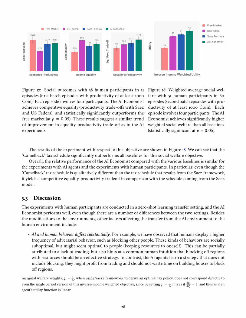
Free Market US Federal Saez Formula AI Economist

Coin

Pro

duce

d

2605

2270

1658

2339

Economic Productivity

Coin

Equ

ality

37%

48%

59%52%

Income Equality

Eq /

Prod

Tra

deof

f

855

1033984

1179

Equality x Productivity

Figure 17: Social outcomes with 58 human participants in 51episodes (first batch episodes with productivity of at least 1000Coin). Each episode involves four participants. The AI Economistachieves competitive equality-productivity trade-offs with Saezand US Federal, and statistically significantly outperforms thefree market (at p = 0.05). These results suggest a similar trendof improvement in equality-productivity trade-off as in the AIexperiments.

Free Market

US Federal

Saez Formula

AI Economist

Utili

ty

24

3736

42

Inverse Income Weighted Utility

Figure 18: Weighted average social wel-fare with 51 human participants in 60episodes (second batch episodes with pro-ductivity of at least 1000 Coin). Eachepisode involves four participants. TheAIEconomist achieves significantly higherweighted social welfare than all baselines(statistically significant at p = 0.05).

The results of the experiment with respect to this objective are shown in Figure 18. We can see that the"Camelback" tax schedule significantly outperforms all baselines for this social welfare objective.

Overall, the relative performance of the AI Economist compared with the various baselines is similar forthe experiments with AI agents and the experiments with human participants. In particular, even though the"Camelback" tax schedule is qualitatively different than the tax schedule that results from the Saez framework,it yields a competitive equality-productivity tradeoff in comparison with the schedule coming from the Saezmodel.

5.3 DiscussionThe experiments with human participants are conducted in a zero-shot learning transfer setting, and the AIEconomist performs well, even though there are a number of differences between the two settings. Besidesthe modifications to the environments, other factors affecting the transfer from the AI environment to thehuman environment include:

• AI and human behavior differs substantially. For example, we have observed that humans display a higherfrequency of adversarial behavior, such as blocking other people. These kinds of behaviors are sociallysuboptimal, but might seem optimal to people (keeping resources to oneself). This can be partiallyattributed to a lack of trading, but also hints at a common human intuition that blocking off regionswith resources should be an effective strategy. In contrast, the AI agents learn a strategy that does notinclude blocking: they might profit from trading and should not waste time on building houses to blockoff regions.

marginal welfare weights, gi = 1zi , when using Saez’s framework to derive an optimal tax policy, does not correspond directly to

even the single period version of this inverse-income weighted objective, since by setting gi = 1zi it is as if

duidxci= 1, and thus as if an

agent’s utility function is linear.

28

• Learning effects. As human participants experiencemultiple episodes, their strategy improves, as observed,for example, through lower average productivity and worse social metrics during qualification rounds.This learning effect is partially controlled for by randomizing the order of tax models presented toparticipants and only using experimental episodes where participants have already participated in oneor more qualification rounds.

• We set the payoff per house for each human agent using a preset skill. For real people, this is not theonly factor that affects the expected average payoff. For instance, people can have different strategies inthe simulation, which affects their average payoff and hence their implied skill. Hence, varying skill andpayoff as a simulation setting only partially emulates the effect of skill on the expected payoff and utilitythat people experience.

Considering all these factors, we find these results for the AI Economist in the presence of humanparticipants encouraging. The AI-driven tax model did not require knowledge of economic theory, did notrequire that we estimate the tax elasticity of labor, and was nevertheless able to learn a well-performingtax policy for use with human participants tabula rasa. We were able to apply the model without requiringrecalibration of tax rates. The only calibration was to scale down the income brackets by a factor of three toadjust for the relative productivity of human and AI agents and enable all income brackets to be exercised.

We emphasize that we do not endorse the particular tax schedule determined by the AI Economist for use in thereal economy.

Still, the encouraging transfer performance suggests there is potential for building AI-driven tax modelsthat can find application to the real world, as a new tool to be used by governments. Moreover, given that theAI tax policy, which is dynamic in that its tax schedule changes across tax periods, substantially outperformsthe Saez formula in the AI simulations, an interesting direction for future research is to develop experimentsthat can inform ways with which dynamic tax models can be applied to human settings.

6 ConclusionWe believe the intersection of machine learning and economics presents a wide range of exciting researchdirections, and gives ample opportunity for new machine learning advances that will have significant positivesocial impact. Our vision for the AI Economist is to enable an objective study of the impact of economicpolicies on real-world economies, at a level of complexity that traditional economics research cannot easilyaddress.

For tax policies in particular, we are hopeful that this kind of research can increase equality and productivityin the real world, helping to promotemore just and healthy economies. We also hope that the AI Economist canfoster transparency, reproducibility, and open and facts-based discussion about applying machine learning toeconomic decision-making, through our public research publications and open-source code. As such, we hopethat future economic AI models can robustly and transparently augment real-world economic policy-makingand in doing so improve social welfare.

In this paper, the economic agents and social planner were trained using model-free RL in AI-based,economic simulations. A key benefit of using model-free RL is flexibility: for instance, any social objective canbe used as the reward function for the planner. Moreover, it does not need any prior world knowledge to finda well-performing tax policy. However, this approach assumes that the inputs and outputs to the agents’ andplanner’s policy models are sufficient and well-defined. For instance, the planner should be able to observe allstate information that is relevant for determining the optimal tax policy. Our initial experiments with humanparticipants suggest that, in our problem setting, the state observed by the planner was sufficient to generalizewell to human agents. In future work, it would be interesting to explore which state information of the real

29

world should be captured by economic simulators to enable generalization of policies from simulation to thereal world.

This work is suggestive of the promise of AI-based, economic simulators for learning economic policieswith the potential to transfer well to the real world. We demonstrated that economic simulators can yieldAI agents with economic behaviors that are consistent with economic intuition, for example agents thatspecialize as a consequence of their inherent skill level. Our experiments also show that policies trained insuch simulators can transfer well to settings with human participants, albeit for our limited problem setting.

Of course, these kinds of economic simulations still have many limitations. They do not yet modelhuman-behavioral factors and interactions between people, including other-regarding utilities, and considera relatively small economy. Moreover, the concept of skill and the associated payoff, as used in our work, isstill a limited representation of economic behavior in the real world. For instance, highly-skilled workersare not paid the same hourly wage across different industries, and skill might be hard to clearly define andmeasure clearly in certain professions. Future simulations could improve the fidelity of simulated economicbehavior by making use of real-world economic data, while advances in large-scale RL and engineering couldincrease the scope of economic simulations.

7 Ethics and Normative AspectsEthics, trust, and transparency are an integral part of Salesforce’s approach to AI research. While the currentversion of the AI Economist provides only a limited representation of the real world, we recognize that itcould be possible to manipulate future, large-scale iterations of the AI Economist to increase inequality andhide this action behind the results of an AI system.

Furthermore, either out of ignorance or malice, bad training data may result in biased recommendations,particularly in cases where users will train the tool using their own data. For instance, the exclusion from themodel of communities and segments of the work-force that are under-represented in training data might leadto bias in AI-driven tax models. This work also opens up the possibility of using richer, observational data toset individual taxation, an area where we anticipate a strong need for robust debate.

Economic simulation enables studying a wide range of economic incentives and their consequences,including models of stakeholder capitalism. However, the simulation used in this work is not an actual toolthat can be currently used with malintent to reconfigure tax policy. We encourage anyone utilizing the AIEconomist to publish a model card and data sheet that describes the ethical considerations of trained AI-driventax models to increase transparency, and by extension, trust, in the system. Furthermore, we believe anyfuture application or policy built on economic simulations should be built on inspectable code and subject tofull transparency.

In order to responsibly publish this research, we have taken the following measures:

• To ensure accountability on our part, we have consulted academic experts on safe release of code andensured we are in compliance with their guidance. We shared the paper and an assessment of the ethicalrisks, mitigation strategies, and assessment of safety to publish with the following external reviewers: Dr.Simon Chesterman, Provost’s Chair and Dean of the National University of Singapore Faculty of Law,and Lofred Madzou, AI Project Lead at the World Economic Forum’s Center for the Fourth IndustrialRevolution. None of the reviewers identified additional ethical concerns or mitigation strategies thatshould be employed. All affirmed that the research is safe to publish.

• To increase transparency, we are publishing this technical paper, as well as a blog post, thereby allowingrobust debate and broad multidisciplinary discussion of our work.

30

• To further promote transparency, we will have a timed open-source release of our environment andsample training code for the simulation. This does not prevent future misuse, but we believe, at thecurrent level of fidelity, transparency is key to promote grounded discussion and future research.

With these mitigation strategies and other considerations in place, we believe this research is safe topublish. Furthermore, this research was not conducted with any corporate or commercial applications inmind.

ReferencesUnited Nations. Inequality Matters: Report of the World Social Situation 2013. 2013. Department of Economicand Social Affairs.

Subu v Subramanian and Ichiro Kawachi. Income inequality and health: What have we learned so far?Epidemiologic Reviews, 26(1):78–91, 2004.

N. Gregory Mankiw, Matthew Weinzierl, and Danny Yagan. Optimal Taxation in Theory and Practice.Journal of Economic Perspectives, 23(4):147–174, December 2009. ISSN 0895-3309. doi: 10.1257/jep.23.4.147. URLhttps://www.aeaweb.org/articles?id=10.1257/jep.23.4.147.

Peter Diamond and Emmanuel Saez. The Case for a Progressive Tax: From Basic Research to PolicyRecommendations. Journal of Economic Perspectives, 25(4):165–190, December 2011. ISSN 0895-3309. doi:10.1257/jep.25.4.165. URL https://www.aeaweb.org/articles?id=10.1257/jep.25.4.165.

Frank P Ramsey. A contribution to the theory of taxation. The Economic Journal, 37(145):47–61, 1927.

Peter A Diamond and James A Mirrlees. Optimal taxation and public production i: Production efficiency. TheAmerican Economic Review, 61(1):8–27, 1971a.

Peter A Diamond and James A Mirrlees. Optimal taxation and public production ii: Tax rules. The AmericanEconomic Review, 61(3):261–278, 1971b.

J. A. Mirrlees. Optimal tax theory: A synthesis. Journal of Public Economics, 6(4):327–358, November 1976. ISSN0047-2727. doi: 10.1016/0047-2727(76)90047-5. URLhttp://www.sciencedirect.com/science/article/pii/0047272776900475.

Emmanuel Saez. Using elasticities to derive optimal income tax rates. The Review of Economic Studies, 68(1):205–229, 2001.

Thomas Piketty and Emmanuel Saez. A theory of optimal inheritance taxation. Econometrica, 81(5):1851–1886,2013.

Thomas Piketty, Emmanuel Saez, and Stefanie Stantcheva. Optimal taxation of top labor incomes: A tale ofthree elasticities. American Economic Journal: Economic Policy, 6(1):230–71, 2014.

Emmanuel Saez and Stefanie Stantcheva. Generalized social marginal welfare weights for optimal tax theory.American Economic Review, 106(1):24–45, 2016.

N Gregory Mankiw. Spreading the wealth around: Reflections inspired by joe the plumber. Eastern EconomicJournal, 36(3):285–298, 2010.

31

N Gregory Mankiw and Matthew Weinzierl. The optimal taxation of height: A case study of utilitarianincome redistribution. American Economic Journal: Economic Policy, 2(1):155–76, 2010.

Mikhail Golosov, Narayana Kocherlakota, and Aleh Tsyvinski. Optimal indirect and capital taxation. TheReview of Economic Studies, 70(3):569–587, 2003.

Narayana R Kocherlakota. Zero expected wealth taxes: A mirrlees approach to dynamic optimal taxation.Econometrica, 73(5):1587–1621, 2005.

Stefania Albanesi and Christopher Sleet. Dynamic optimal taxation with private information. The Review ofEconomic Studies, 73(1):1–30, 2006.

Narayana R. Kocherlakota. The New Dynamic Public Finance. Princeton University Press, stu - student editionedition, 2010. ISBN 978-0-691-13915-9. URL www.jstor.org/stable/j.ctt7s9rn.

Jon Gruber and Emmanuel Saez. The elasticity of taxable income: Evidence and implications. Journal ofPublic Economics, 84(1):1–32, 2002.

Raj Chetty. Bounds on elasticities with optimization frictions: A synthesis of micro and macro evidence onlabor supply. Econometrica, 80(3):969–1018, 2012.

Jessica Goldberg. Kwacha gonna do? experimental evidence about labor supply in rural malawi. AmericanEconomic Journal: Applied Economics, 8(1):129–49, 2016.

Joel Slemrod. High-income families and the tax changes of the 1980s: The anatomy of behavioral response. InEmpirical Foundations of Household Taxation, pages 169–192. University of Chicago Press, 1996.

Austan Goolsbee. What happens when you tax the rich? evidence from executive compensation. Journal ofPolitical Economy, 108(2):352–378, 2000.

Alberto Alesina, Edward Glaeser, and Bruce Sacerdote. Work and leisure in the united states and europe:Why so different? NBER Macroeconomics Annual, 20:1–64, 2005.

Edward J McCaffery and Joel Slemrod. Behavioral Public Finance. Russell Sage Foundation, 2006.

Ilyana Kuziemko, Michael I Norton, Emmanuel Saez, and Stefanie Stantcheva. How elastic are preferencesfor redistribution? evidence from randomized survey experiments. American Economic Review, 105(4):1478–1508, 2015.

Alberto Alesina, Stefanie Stantcheva, and Edoardo Teso. Intergenerational mobility and preferences forredistribution. American Economic Review, 108(2):521–54, 2018.

John H Holland and John H Miller. Artificial adaptive agents in economic theory. The American EconomicReview, 81(2):365–370, 1991.

Eric Bonabeau. Agent-based modeling: Methods and techniques for simulating human systems. Proceedings ofthe National Academy of Sciences, 99(suppl 3):7280–7287, May 2002. ISSN 0027-8424, 1091-6490. doi:10.1073/pnas.082080899. URL https://www.pnas.org/content/99/suppl_3/7280.

W. Brian Arthur. Designing Economic Agents that Act like Human Agents: A Behavioral Approach toBounded Rationality. The American Economic Review, 81(2):353–359, 1991. ISSN 0002-8282. URLhttps://www.jstor.org/stable/2006884.

32

J. Doyne Farmer and Duncan Foley. The economy needs agent-based modelling. Nature, 460(7256):685–686,August 2009. ISSN 1476-4687. doi: 10.1038/460685a. URL https://www.nature.com/articles/460685a.

Kim Bloomquist. Tax Compliance as an Evolutionary Coordination Game: An Agent-Based Approach. PublicFinance Review, 39(1):25–49, 2011. URL https:

//econpapers.repec.org/article/saepubfin/v_3a39_3ay_3a2011_3ai_3a1_3ap_3a25-49.htm.

Francisco J. Miguel, José A. Noguera, Toni Llacer, and Eduardo Tapia. Exploring Tax Compliance: AnAgent-Based Simulation. In Ecms, 2012. doi: 10.7148/2012-0638-0643.

Shree Krishna Subburaj and Shrisha Rao. Theory and Agent-based Modeling of Taxpayer Preference andBehavior. In Proceedings of the 22Nd International Symposium on Distributed Simulation and Real TimeApplications, DS-RT ’18, pages 163–172, Piscataway, NJ, USA, 2018. IEEE Press. ISBN 978-1-5386-5048-6. URLhttp://dl.acm.org/citation.cfm?id=3330299.3330319. event-place: Madrid, Spain.

Nicolás Garrido and Luigi Mittone. An agent based model for studying optimal tax collection policy usingexperimental data: The cases of Chile and Italy. The Journal of Socio-Economics, 42:24–30, February 2013.ISSN 1053-5357. doi: 10.1016/j.socec.2012.11.002. URLhttp://www.sciencedirect.com/science/article/pii/S105353571200114X.

Guillaume J. Laurent, Laëtitia Matignon, and N. Le Fort-Piat. The World of Independent Learners is NotMarkovian. Int. J. Know.-Based Intell. Eng. Syst., 15(1):55–64, January 2011. ISSN 1327-2314. URLhttp://dl.acm.org/citation.cfm?id=1971886.1971887.

Richard S. Sutton and Andrew G. Barto. Reinforcement Learning: An Introduction. MIT Press, October 2018a.ISBN 978-0-262-35270-3. Google-Books-ID: uWV0DwAAQBAJ.

Caroline Claus and Craig Boutilier. The Dynamics of Reinforcement Learning in Cooperative MultiagentSystems. In Proceedings of the Fifteenth National/Tenth Conference on Artificial Intelligence/InnovativeApplications of Artificial Intelligence, AAAI ’98/IAAI ’98, pages 746–752, Menlo Park, CA, USA, 1998. AmericanAssociation for Artificial Intelligence. ISBN 978-0-262-51098-1. URLhttp://dl.acm.org/citation.cfm?id=295240.295800.

Trapit Bansal, Jakub Pachocki, Szymon Sidor, Ilya Sutskever, and Igor Mordatch. Emergent Complexity viaMulti-Agent Competition. arXiv:1710.03748 [Cs], October 2017. URLhttp://arxiv.org/abs/1710.03748. arXiv: 1710.03748.

Max Jaderberg, Wojciech M. Czarnecki, Iain Dunning, Luke Marris, Guy Lever, Antonio Garcia Castaneda,Charles Beattie, Neil C. Rabinowitz, Ari S. Morcos, Avraham Ruderman, Nicolas Sonnerat, Tim Green,Louise Deason, Joel Z. Leibo, David Silver, Demis Hassabis, Koray Kavukcuoglu, and Thore Graepel.Human-level performance in first-person multiplayer games with population-based deep reinforcementlearning. arXiv:1807.01281 [Cs, Stat], July 2018. URL http://arxiv.org/abs/1807.01281. arXiv:1807.01281.

OpenAI. Openai five. https://blog.openai.com/openai-five/, 2018.

Ryan Lowe, Yi Wu, Aviv Tamar, Jean Harb, Pieter Abbeel, and Igor Mordatch. Multi-Agent Actor-Critic forMixed Cooperative-Competitive Environments. arXiv:1706.02275 [Cs], June 2017. URLhttp://arxiv.org/abs/1706.02275. arXiv: 1706.02275.

33

Andrea Tacchetti, H. Francis Song, Pedro A. M. Mediano, Vinicius Zambaldi, Neil C. Rabinowitz, ThoreGraepel, Matthew Botvinick, and Peter W. Battaglia. Relational Forward Models for Multi-Agent Learning.arXiv:1809.11044 [Cs, Stat], September 2018. URL http://arxiv.org/abs/1809.11044. arXiv: 1809.11044.

Tianmin Shu and Yuandong Tian. M^3rl: Mind-aware Multi-agent Management Reinforcement Learning.arXiv:1810.00147 [Cs, Stat], September 2018. URL http://arxiv.org/abs/1810.00147. arXiv: 1810.00147.

Peter Sunehag, Guy Lever, Audrunas Gruslys, Wojciech Marian Czarnecki, Vinicius Zambaldi, Max Jaderberg,Marc Lanctot, Nicolas Sonnerat, Joel Z. Leibo, Karl Tuyls, and Thore Graepel. Value-DecompositionNetworks For Cooperative Multi-Agent Learning. arXiv:1706.05296 [Cs], June 2017. URLhttp://arxiv.org/abs/1706.05296. arXiv: 1706.05296.

Jakob N. Foerster, Richard Y. Chen, Maruan Al-Shedivat, Shimon Whiteson, Pieter Abbeel, and IgorMordatch. Learning with Opponent-Learning Awareness. arXiv:1709.04326 [Cs], September 2017. URLhttp://arxiv.org/abs/1709.04326. arXiv: 1709.04326.

Alexander Peysakhovich and Adam Lerer. Prosocial learning agents solve generalized Stag Hunts better thanselfish ones. arXiv:1709.02865 [Cs], September 2017. URL http://arxiv.org/abs/1709.02865. arXiv:1709.02865.

Edward Hughes, Joel Z. Leibo, Matthew G. Phillips, Karl Tuyls, Edgar A. Duéñez Guzmán, Antonio GarcíaCastañeda, Iain Dunning, Tina Zhu, Kevin R. McKee, Raphael Koster, Heather Roff, and Thore Graepel.Inequity aversion improves cooperation in intertemporal social dilemmas. arXiv:1803.08884 [Cs, Q-Bio],March 2018. URL http://arxiv.org/abs/1803.08884. arXiv: 1803.08884.

Alistair Letcher, Jakob Foerster, David Balduzzi, Tim Rocktäschel, and Shimon Whiteson. Stable OpponentShaping in Differentiable Games. arXiv:1811.08469 [Cs], November 2018. URLhttp://arxiv.org/abs/1811.08469. arXiv: 1811.08469.

David Balduzzi, Sebastien Racaniere, James Martens, Jakob Foerster, Karl Tuyls, and Thore Graepel. TheMechanics of n-Player Differentiable Games. arXiv:1802.05642 [Cs], February 2018. URLhttp://arxiv.org/abs/1802.05642. arXiv: 1802.05642.

Joel Z. Leibo, Vinicius Zambaldi, Marc Lanctot, Janusz Marecki, and Thore Graepel. Multi-agentReinforcement Learning in Sequential Social Dilemmas. arXiv:1702.03037 [Cs], February 2017. URLhttp://arxiv.org/abs/1702.03037. arXiv: 1702.03037.

David Mguni, Joel Jennings, Sergio Valcarcel Macua, Emilio Sison, Sofia Ceppi, and Enrique Munoz de Cote.Coordinating the Crowd: Inducing Desirable Equilibria in Non-Cooperative Systems. arXiv:1901.10923 [Cs],January 2019. URL http://arxiv.org/abs/1901.10923. arXiv: 1901.10923.

Natasha Jaques, Angeliki Lazaridou, Edward Hughes, Caglar Gulcehre, Pedro A. Ortega, D. J. Strouse, Joel Z.Leibo, and Nando de Freitas. Social Influence as Intrinsic Motivation for Multi-Agent Deep ReinforcementLearning. arXiv:1810.08647 [Cs, Stat], October 2018. URL http://arxiv.org/abs/1810.08647. arXiv:1810.08647.

V. Conitzer and T. Sandholm. Complexity of mechanism design. In Proceedings of the 18th Conference onUncertainty in Artificial Intelligence, pages 103–110, 2002.

V. Conitzer and T. Sandholm. Self-interested automated mechanism design and implications for optimalcombinatorial auctions. In Proceedings of the 5th ACM Conference on Electronic Commerce, pages 132–141,2004.

34

Y. Cai, C. Daskalakis, and S. M. Weinberg. An algorithmic characterization of multi-dimensional mechanisms.In Proceedings of the 44th ACM Symposium on Theory of Computing, pages 459–478, 2012a.

Y. Cai, C. Daskalakis, and M. S. Weinberg. Optimal multi-dimensional mechanism design: Reducing revenueto welfare maximization. In Proceedings of the 53rd IEEE Symposium on Foundations of Computer Science,pages 130–139, 2012b.

Y. Cai, C. Daskalakis, and S. M. Weinberg. Understanding incentives: Mechanism design becomes algorithmdesign. In Proceedings of the 54th IEEE Symposium on Foundations of Computer Science, pages 618–627, 2013.

Paul Dütting, Zhe Feng, Harikrishna Narasimhan, David C. Parkes, and Sai Srivatsa Ravindranath. OptimalAuctions through Deep Learning. In Proc. 36th Int. Conf. On Machine Learning, pages 1706–1715, 2019.

Z. Feng, H. Narasimhan, and D. C. Parkes. Deep learning for revenue-optimal auctions with budgets. InProceedings of the 17th International Conference on Autonomous Agents and Multiagent Systems, pages 354–362,2018.

A. Tacchetti, D.J. Strouse, M. Garnelo, T. Graepel, and Y. Bachrach. A neural architecture for designingtruthful and efficient auctions. CoRR, abs/1907.05181, 2019.

W. Shen, P. Tang, and S. Zuo. Automated mechanism design via neural networks. In Proceedings of the 18thInternational Conference on Autonomous Agents and Multiagent Systems, 2019. Forthcoming.

N. Golowich, H. Narasimhan, and D. C. Parkes. Deep learning for multi-facility location mechanism design.In Proceedings of the 27th International Joint Conference on Artificial Intelligence, pages 261–267, 2018.

P. Dütting, F. Fischer, P. Jirapinyo, J. Lai, B. Lubin, and D. C. Parkes. Payment rules throughdiscriminant-based classifiers. ACM Transactions on Economics and Computation, 3(1):5, 2014.

R. Cole and T. Roughgarden. The sample complexity of revenue maximization. In Proceedings of the 46thACM Symposium on Theory of Computing, pages 243–252, 2014.

J. Morgenstern and T. Roughgarden. On the pseudo-dimension of nearly optimal auctions. In Proceedings ofthe 28th Conference on Neural Information Processing Systems, pages 136–144, 2015.

M-F. Balcan, T. Sandholm, and E. Vitercik. Sample complexity of automated mechanism design. InProceedings of the 29th Conference on Neural Information Processing Systems, pages 2083–2091, 2016.

Y. A. Gonczarowski and S. M. Weinberg. The sample complexity of up-to-epsilon multi-dimensional revenuemaximization. In 59th IEEE Annual Symposium on Foundations of Computer Science, pages 416–426, 2018.

A. D. Procaccia, A. Zohar, Y. Peleg, and J. S. Rosenschein. Artificial Intelligence, 173:1133–1149, 2009.

H. Narasimhan, S. Agarwal, and D. C. Parkes. Automated mechanism design without money via machinelearning. In Proceedings of the 25th International Joint Conference on Artificial Intelligence, pages 433–439, 2016.

H. Narasimhan and D. C. Parkes. A general statistical framework for designing strategy-proof assignmentmechanisms. In Proceedings of the Conference on Uncertainty in Artificial Intelligence, 2016.

Andrew Byde. Applying evolutionary game theory to auction mechanism design. In Daniel A. Menascé andNoam Nisan, editors, Proceedings 4th ACM Conference on Electronic Commerce (EC-2003), San Diego,California, USA, June 9-12, 2003, pages 192–193. ACM, 2003. doi: 10.1145/779928.779954. URLhttps://doi.org/10.1145/779928.779954.

35

Steve Phelps, Peter McBurney, Simon Parsons, and Elizabeth Sklar. Co-evolutionary auction mechanismdesign: A preliminary report. In Julian A. Padget, Onn Shehory, David C. Parkes, Norman M. Sadeh, andWilliam E. Walsh, editors, Agent-Mediated Electronic Commerce IV, Designing Mechanisms and Systems,AAMAS 2002 Workshop on Agent Mediated Electronic Commerce, Bologna, Italy, July 16, 2002, Revised Papers,volume 2531 of Lecture Notes in Computer Science, pages 123–142. Springer, 2002. doi:10.1007/3-540-36378-5\_8. URL https://doi.org/10.1007/3-540-36378-5_8.

Steve Phelps, Peter McBurney, and Simon Parsons. Evolutionary mechanism design: A review. AutonomousAgents and Multi-Agent Systems, 21(2):237–264, 2010. doi: 10.1007/s10458-009-9108-7. URLhttps://doi.org/10.1007/s10458-009-9108-7.

James Pita, Manish Jain, Janusz Marecki, Fernando Ordóñez, Christopher Portway, Milind Tambe, CraigWestern, Praveen Paruchuri, and Sarit Kraus. Deployed ARMOR protection: The application of a gametheoretic model for security at the los angeles international airport. In Michael Berger, Bernard Burg, andSatoshi Nishiyama, editors, 7th International Joint Conference on Autonomous Agents and Multiagent Systems(AAMAS 2008), Estoril, Portugal, May 12-16, 2008, Industry and Applications Track Proceedings, pages 125–132.IFAAMAS, 2008. URL https://dl.acm.org/citation.cfm?id=1402819.

Milind Tambe. Security and Game Theory - Algorithms, Deployed Systems, Lessons Learned. CambridgeUniversity Press, 2012. ISBN 978-1-10-709642-4. URL http://www.cambridge.org/de/academic/

subjects/computer-science/communications-information-theory-and-security/

security-and-game-theory-algorithms-deployed-systems-lessons-learned?format=AR.

Yufei Wang, Zheyuan Ryan Shi, Lantao Yu, Yi Wu, Rohit Singh, Lucas Joppa, and Fei Fang. Deepreinforcement learning for green security games with real-time information. In The Thirty-Third AAAIConference on Artificial Intelligence, AAAI 2019, the Thirty-First Innovative Applications of Artificial IntelligenceConference, IAAI 2019, the Ninth AAAI Symposium on Educational Advances in Artificial Intelligence, EAAI2019, Honolulu, Hawaii, USA, January 27 - February 1, 2019, pages 1401–1408. AAAI Press, 2019. doi:10.1609/aaai.v33i01.33011401. URL https://doi.org/10.1609/aaai.v33i01.33011401.

Sanket Shah, Arunesh Sinha, Pradeep Varakantham, Andrew Perrault, and Milind Tambe. Solving onlinethreat screening games using constrained action space reinforcement learning. CoRR, abs/1911.08799, 2019.URL http://arxiv.org/abs/1911.08799.

Christos Dimitrakakis, David C. Parkes, Goran Radanovic, and Paul Tylkin. Multi-view decision processes:The helper-ai problem. In Isabelle Guyon, Ulrike von Luxburg, Samy Bengio, Hanna M. Wallach, RobFergus, S. V. N. Vishwanathan, and Roman Garnett, editors, Advances in Neural Information ProcessingSystems 30: Annual Conference on Neural Information Processing Systems 2017, 4-9 December 2017, Long Beach,CA, USA, pages 5443–5452, 2017. URL http:

//papers.nips.cc/paper/7128-multi-view-decision-processes-the-helper-ai-problem.

Micah Carroll, Rohin Shah, Mark K. Ho, Tom Griffiths, Sanjit A. Seshia, Pieter Abbeel, and Anca D. Dragan.On the utility of learning about humans for human-ai coordination. In Hanna M. Wallach, Hugo Larochelle,Alina Beygelzimer, Florence d’Alché-Buc, Emily B. Fox, and Roman Garnett, editors, Advances in NeuralInformation Processing Systems 32: Annual Conference on Neural Information Processing Systems 2019, NeurIPS2019, 8-14 December 2019, Vancouver, BC, Canada, pages 5175–5186, 2019. URL http://papers.nips.cc/

paper/8760-on-the-utility-of-learning-about-humans-for-human-ai-coordination.

Paul Tylkin, David C. Parkes, and Goran Radanovic. Multi-player Atari: Designing Helper-AIs in RichEnvironments. Technical report, Harvard University, 2020.

36

David Balduzzi, Marta Garnelo, Yoram Bachrach, Wojciech Czarnecki, Julien Pérolat, Max Jaderberg, andThore Graepel. Open-ended learning in symmetric zero-sum games. In Kamalika Chaudhuri and RuslanSalakhutdinov, editors, Proceedings of the 36th International Conference on Machine Learning, ICML 2019, 9-15June 2019, Long Beach, California, USA, volume 97 of Proceedings of Machine Learning Research, pages434–443. PMLR, 2019. URL http://proceedings.mlr.press/v97/balduzzi19a.html.

Pingzhong Tang. Reinforcement mechanism design. In Carles Sierra, editor, Proceedings of the Twenty-SixthInternational Joint Conference on Artificial Intelligence, IJCAI 2017, Melbourne, Australia, August 19-25, 2017,pages 5146–5150. ijcai.org, 2017. doi: 10.24963/ijcai.2017/739. URLhttps://doi.org/10.24963/ijcai.2017/739.

Weiran Shen, Binghui Peng, Hanpeng Liu, Michael Zhang, Ruohan Qian, Yan Hong, Zhi Guo, Zongyao Ding,Pengjun Lu, and Pingzhong Tang. Reinforcement mechanism design, with applications to dynamic pricingin sponsored search auctions. In AAAI Conference on Artificial Intelligence (AAAI 2020), 2020.

David R. M. Thompson, Neil Newman, and Kevin Leyton-Brown. The positronic economist: Acomputational system for analyzing economic mechanisms. In Satinder P. Singh and Shaul Markovitch,editors, Proceedings of the Thirty-First AAAI Conference on Artificial Intelligence, February 4-9, 2017, SanFrancisco, California, USA, pages 720–727. AAAI Press, 2017. URLhttp://aaai.org/ocs/index.php/AAAI/AAAI17/paper/view/14648.

Yevgeniy Vorobeychik, Daniel M. Reeves, and Michael P. Wellman. Constrained automated mechanismdesign for infinite games of incomplete information. Autonomous Agents and Multi-Agent Systems, 25(2):313–351, 2012. doi: 10.1007/s10458-011-9177-2. URL https://doi.org/10.1007/s10458-011-9177-2.

Benedikt Bünz, Benjamin Lubin, and Sven Seuken. Designing core-selecting payment rules: A computationalsearch approach. In Éva Tardos, Edith Elkind, and Rakesh Vohra, editors, Proceedings of the 2018 ACMConference on Economics and Computation, Ithaca, NY, USA, June 18-22, 2018, page 109. ACM, 2018. doi:10.1145/3219166.3219206. URL https://doi.org/10.1145/3219166.3219206.

David C. Parkes and Michael P. Wellman. Economic reasoning and artificial intelligence. Science, 349(6245):267–272, July 2015. ISSN 0036-8075, 1095-9203. doi: 10.1126/science.aaa8403. URLhttp://science.sciencemag.org/content/349/6245/267.

Richard S Sutton and Andrew G Barto. Reinforcement Learning: An Introduction. MIT Press, October 2018b.ISBN 978-0-262-35270-3. Google-Books-ID: uWV0DwAAQBAJ.

Gerard Debreu. Representation of a preference ordering by a numerical function. Readings in MathematicalEconomics, 1, 1968.

Ronald J Williams and Jing Peng. Function optimization using connectionist reinforcement learningalgorithms. Connection Science, 3(3):241–268, 1991.

Volodymyr Mnih, Adria Puigdomenech Badia, Mehdi Mirza, Alex Graves, Timothy Lillicrap, Tim Harley,David Silver, and Koray Kavukcuoglu. Asynchronous methods for deep reinforcement learning. InInternational Conference on Machine Learning, pages 1928–1937, 2016.

Eric Liang, Richard Liaw, Philipp Moritz, Robert Nishihara, Roy Fox, Ken Goldberg, Joseph E. Gonzalez,Michael I. Jordan, and Ion Stoica. RLlib: Abstractions for Distributed Reinforcement Learning. 35thInternational Conference on Machine Learning, ICML 2018, 7:4768–4780, 2018.

37

John Schulman, Filip Wolski, Prafulla Dhariwal, Alec Radford, and Oleg Klimov. Proximal policyoptimization algorithms. arXiv preprint arXiv:1707.06347, 2017.

Diederik Kingma and Jimmy Ba. Adam: A Method for Stochastic Optimization. arXiv:1412.6980 [Cs],December 2014. URL http://arxiv.org/abs/1412.6980. arXiv: 1412.6980.

A Details of EnvironmentThis section provides a more exhaustive description of the environment dynamics and the observations (and,where appropriate, actions) available to agents and the social planner. We describe these separately for each ofthe mechanics used to construct the simulation. Note that observations and actions are essentially the inputsand outputs of the neural network policies trained using RL. Planner observations/actions are irrelevant forbaseline tax models, where tax rates are either fixed or calculated formulaically.

World Dynamics. The Gather-and-Build environment is organized over a 2D grid. Grid cells can beoccupied by agents, resources, houses, or other landmarks such as water. At the start of each episode, certaincells are designated as ‘source’ cells that function to spawn new resource units.10 A given source cell onlyspawns a single type of resource, i.e. wood or stone. If an agent moves to a cell that contains a resource, thatresource is added to the agent’s inventory and removed from the world at that location. At the start of eachtimestep, resources randomly re-spawn at empty source cells according to the regeneration probability.

The state of the world is represented as a H ×W ×C tensor, where H andW are the size of the world andC is the number of unique entities that may occupy a cell, and the value of a given element indicates that aparticular entity is occupying the associated location. The social planner is able to observe the full world statetensor, while agent observations are restricted to views of the state tensor from a narrower, egocentric spatialwindow. Our experiments use a world of size 25-by-25, where agent observations have size 11-by-11. Agentspatial observations are padded as needed when their observation window extends beyond the world grid.

Movement and Gathering. Agents must navigate the world in order to collect resources and build newhouses. The action space of the agents includes 4 actions for moving up, down, left, and right. Agents arerestricted from moving on top of water cells, cells occupied by other agents, and cells containing houses builtby other agents. In this way, agents may create difficulty for other agents by restricting their available paths.

Before resources may be sold or used to build houses, they must be collected from the world. An agentcollects resources by moving itself on top of a resource-populated source cell. By default, this adds a singleunit of the collected resources to the agent’s inventory, with the possibility of a bonus unit also being collected,the probability of which is determined by the agent’s collecting skill.

Agents observe the state of their inventories (including wood, stone, and coin) as well as their owncollecting skill. The planner is also able to observe agents’ inventories but cannot observe skill values.

Building. When an agent has both stone and wood in its inventory, it may spend one unit of each in orderto construct a house. The action space of the agents includes 1 action for building. Agents are restrictedfrom building on source cells as well as locations where a house already exists. Building places a house at thelocation occupied by the agent and adds coin to the agent’s inventory, the amount of which is determined byits building skill. Agents observe their own building skill, which the planner is not able to observe.

10For our purposes, we use the same, fixed layout of source cells each episode.

38

Trading. Agents can buy and sell resources from one another through a trading mechanism structured as acontinuous double auction. This is conceptually similar to a commodities or stock exchange, where participantsdo not interface directly but instead submit bids and asks to a market, which identifies and executes validtrades. The action space of the agents includes 44 actions for trading, representing the combination of 11price levels (0, . . . , 10 coin), 2 directions (bids and asks), and 2 resources (wood and stone). Note: agents buyresources by submitting bids and sell resources by submitting asks. Each trade action therefore maps to asingle order (i.e. bid 3 coin for 1 wood, ask for 5 coin in exchange for 1 stone, etc.). Once an order is submitted,it remains open until either it is matched (in which case a trade occurs) or it expires (after 50 timesteps). Agentsare restricted from having more than 5 open orders for each resource and are restricted from placing ordersthat they cannot complete: they cannot bid with more coin than they possess and cannot submit asks forresources that they do not have.

A bid/ask pair form a valid trade if they are for the same resource and the bid price matches or exceedsthe ask price. When a new order is received (i.e. bid 3 coin for 1 wood) it is compared against complementaryorders to identify potential valid trades. When a single bid (ask) could be paired with multiple existing asks(bids), priority is giving the ask (bid) with the lowest (highest) price; in the event of ties, priority then is givento the oldest existing order. Once a match is identified, the trade is executed using the price of whicheverorder was placed first. As an example, if the market receives a new bid that offers 8 coin for 1 stone and themarket has two open asks offering 1 stone for 3 coin and 1 stone for 7 coin, respectively, the market would pairthe bid with the first ask and a trade would be executed for 1 stone at a price of 3 coin: the bidding agent loses3 coin and gains 1 stone and the asking agent loses 1 stone and gains 3 coin. Once a bid and ask are paired andthe trade is executed, both orders are removed from the market.

The state of the market is captured by the number of outstanding bids and asks at each price level for eachresource. Agents observe these counts both for their own bids/asks as well as the cumulative bids/asks ofother agents (representing the bids/asks that they could respond to). The planner observes the cumulativebids/asks of all agents. In addition, both agents and the planner observe some historical information from themarket: (for each resource) the average trading price as well as the number of trades at each price level.

Taxation and Redistribution. The main text describes the general implementation of periodic, bracketedtaxes used in our environment (Section 3.1). On the first timestep of each tax period, the planner sets themarginal tax rates that will be used to collect taxes when the tax period ends. For baseline models, theseare set either formulaically or using fixed rates. For taxes controlled by a deep neural network (i.e. AIEconomist), the action space of the planner is divided into seven action subspaces, one for each tax bracket:{0, 0.05, 0.10, . . . , 1.0}7. Each subspace denotes the set of discretized marginal tax rates that the planner mayselect.11 The action space takes this form because, when setting new rates, the planner samples 7 rates at once.

Agents observe:

• The tax rates of the current tax period

• The marginal rate at the income level earned within the current period so far

• Indicators of the temporal progress of the current tax period

• The set of sorted and anonymized incomes the agents reported in the previous period

The planner observes the same information as well as the non-anonymized income and marginal tax rate (atthat income) of each agent in the previous period.

11Discretization of tax rates only applies to deep learning networks.

39

Action Details. In our implementation, both agents and planners use discrete action spaces. One advantageof this choice is that it grants easier control over which actions the agent/planner models can sample at a giventime. We encode this using ‘action masks’ which we use to ensure that the policy network assigns effectively 0probability to restricted actions. Action masking is useful for preventing invalid actions and is how we controlthe tax annealing (see Section 4.2) for the AI Economist experiments.

In addition to the actions described above, we include a NO-OP action (“no operation”) in each action space.(For the planner, each of the 7 action subspaces includes a NO-OP action.) The NO-OP action is interpreted asessentially taking no action, allowing the agent to “idle” and the planner to leave a bracket’s tax rates unchangedbetween periods.

Most importantly, we use these implementation features to enable the planner to observe every timestepwhile only acting at the start of each new tax period. For timesteps other than those at the start of a tax periodwe simply use the action mask to enforce that only NO-OP actions are sampled. This allows the planner touse rich temporal information while also ensuring that policy gradients are only propagated from the actionsamples used to control taxes.

B Training Hyperparameters and Experiment SettingsFor each experiment, experience collection was parallelized over 60 replicas of the environment. Each trainingiteration involved collecting h steps from each replica (using the latest policy parameters), followed by around of parameter updates using the collected samples. With a sampling horizon of 200 timesteps and60 environment replicas, a total of 12000 timesteps were sampled per training iteration. Since each “agent”experiences its transition per timestep, this is actually a total of 60000 transitions: 48000 for the 4 agents and12000 for the planner. When doing policy updates, we divided each such set of transitions into minibatchesof size 3000 and perform one gradient update per minibatch. Therefore, each training iteration involved 16updates to the agent parameters and 4 to the planner parameters. We use PPO to accomodate multiple updatesper training iteration.

Tables 2 and 3 provide details regarding the training hyperparameters and environment settings, respec-tively, used in our AI experiments.

C Details on Experiments with Human ParticipantsAll experiment modules used with human participants are shown and described in Figures 19 (lobby, tutorial),20 (main graphical interface), and 21 (survey).

40

Parameter ValueTraining algorithm ppoNumber of parallel environment replicas 60Sampling horizon (steps per replica) h 200SGD minibatch size 3000SGD sequence length 50Policy updates per horizon (agent) 16Policy updates per horizon (planner) 4CPUs 15GPUs 2Learning rate (agent) 0.0003Learning rate (planner) 0.0001Entropy regularization coefficient (agent) 0.025Entropy regularization coefficient (planner) 0.1Gamma γ 0.998GAE lambda 0.98Gradient clipping 10Value function loss coefficient 0.05Number of convolutional layers 2Number of fully-connected layers 2Fully-connected layer dimension (agent) 128Fully-connected layer dimension (planner) 256LSTM cell size (agent) 128LSTM cell size (planner) 256All agents share weights TrueValue/Policy networks share weights FalsePlanner gets spatial info TrueAgents get full spatial observation FalseAgent spatial observation box half-width 5Phase one training duration 50M stepsPhase two training duration 400M stepsPhase two initial max τ 10%Phase two tax annealing duration 54M steps

Table 2: Training hyperparameters.

41

Algorithm 1 Inner-Outer Loop Reinforcement Learning. Economic agents and social planner learn simulta-neously. Bold-faced symbols indicate quantities for multiple agents. Note that agents share weights.Require: Sampling horizon h, tax period length MRequire: On-policy learning algorithm A (for instance, A3C, PPO)Require: Stopping criterion C (for instance, agent and planner rewards have not improved)Ensure: Trained agent and planner policy weights θ, ϕs, o, op, h, hp ⇐ s0, o0, op,0, h0, hp,0 . Reset episodeθ, ϕ⇐ θ0, ϕ0 . Initial agent and planner policy weightsD,Dp ⇐ {}, {} . Reset agent and planner transition bufferswhile training do

for t = 1, . . . ,h doa, h⇐ π(·|o, h, θ) . Sample agent actions; update hidden stateif t mod M = 0 then . First timestep of tax period

τ, hp ⇐ πp(·|op, hp, ϕ) . Sample marginal tax rates; update planner hidden stateelse

no-op, hp ⇐ πp(·|op, hp, ϕ) . Only update planner hidden stateend ifs′, o′, o′p, r, rp ⇐ Env.step(s, a, τ) . Next state / observations, pre-tax reward, planner rewardif t mod M = M-1 then . Last timestep of tax period

s′, o′, o′p, r, rp ⇐ Env.tax(s′, τ) . Apply taxes; compute post-tax rewardsend ifD ⇐ D ∪ {(o, a, r, o′)} . Update agent transition bufferDp ⇐ Dp ∪ {(op, τ, rp, o′p)} . Update planner transition buffers, o, op ⇐ s′, o′, o′p

end forUpdate θ, ϕ using data in D,Dp and A.D,Dp ⇐ {}, {} . Reset agent and planner transition buffersif episode is completed then

s, o, op, h, hp ⇐ s0, o0, op,0, h0, hp,0 . Reset episodeend ifif criterion C is met then return θ, ϕend if

end while

42

Parameter ValueNumber of agents N 4Episode length H 1000World height 25World width 25Resource respawn probability 0.01Max resource health 1Skill distribution paretoStarting agent coin xci,0 0Iso-elastic utility exponent η 0.23Move labor 0.21Gather labor 0.21Trade labor 0.05Build labor 2.1Minimum build payout 10Build payment max skill multiplier 3House lifetime infMax bid/ask price 10Max bid/ask order duration 50Max number of open orders per resource 5Tax period duration M 100Min bracket rate 0%Max bracket rate 100%Rate discretization (AI Economist) 5%Bracket cutoffs {m0, . . . ,mB} us-federalsocial welfare weights (Saez formula) gi inverse-income

Table 3: Environment settings.

43

Figure 19: The starting point for each experiment was the lobby and tutorial (Figure 19). The tutorial explainedall rules of the world and the objective for each participant. It also explained how the variable part of paymentfor the experiment was computed. In addition, an example of the graphical interface and keyboard controlswas shown. Participants were warned not to idle in the game. Participants were given 2 minutes before thestart of the experiment to read the tutorial. After this initial period, as soon as there were enough participantsto form a group, the lobby system presented the participants in the new group with the experiment’s mainpage.

44

Figure 20: The main experiment’s graphical user interface (Figure 20) showed (from top to bottom): theendowment of the agent, the remaining time in the episode, the bonus amount earned so far, the spatialstate of the world, the tax information and current tax rate, the time left, the number of houses built and thenumber of profitable houses left to build. Below all data, a reminder of the controls was shown as well. Afteran episode was over, participants were returned to the lobby (if the participant had seen less than 4 episodes)or survey (if 4 episodes had been seen).

45

Figure 21: The post-experiment survey showed how much the participant had collected in terms of resources,coin and bonus. It also asked questions about the participants experience, strategy and general feedback onthe experiment. For instance, participants could communicate technical issues, such as lag. At the end of thesurvey, participants were given a confirmation code that allowed them to confirm successful completion ofthe task on the Amazon Mechanical Turk platform.

46