the word-space model - sicseprints.sics.se/437/1/thewordspacemodel.pdf · the word-space model is a...

The Word-Space Model

Using distributional analysis to represent

syntagmatic and paradigmatic relations between words

in high-dimensional vector spaces

Magnus Sahlgren

A Dissertation submitted to Stockholm University

in partial fulfillment of the requirements

for the degree of Doctor of Philosophy

2006

Stockholm University National Graduate School Swedish Institute

Department of Linguistics of Language Technology of Computer Science

Computational Linguistics Gothenburg University Userware Laboratory

Stockholm, Sweden Gothenburg, Sweden Kista, Sweden

ISBN 91-7155-281-2 ISSN 1101-1335

ISRN SICS-D–44–SE

SICS Dissertation Series 44

Doctoral Dissertation

Department of Linguistics

Stockholm University

c© Magnus Sahlgren, 2006.

ISBN Nr 91-7155-281-2

This thesis was typeset by the author using LATEX

Printed by Universitetsservice US-AB, Sweden, 2006.

Bart: Look at me, I’m a grad student! I’m thirtyyears old and I made $600 last year!

Marge: Bart, don’t make fun of grad students!They just made a terrible life choice.

(The Simpsons, Episode “Home Away from Homer”)

Abstract

The word-space model is a computational model of word meaning that utilizes thedistributional patterns of words collected over large text data to represent seman-tic similarity between words in terms of spatial proximity. The model has beenused for over a decade, and has demonstrated its mettle in numerous experimentsand applications. It is now on the verge of moving from research environmentsto practical deployment in commercial systems. Although extensively used andintensively investigated, our theoretical understanding of the word-space model re-mains unclear. The question this dissertation attempts to answer is what kind ofsemantic information does the word-space model acquire and represent?

The answer is derived through an identification and discussion of the threemain theoretical cornerstones of the word-space model: the geometric metaphorof meaning, the distributional methodology, and the structuralist meaning theory.It is argued that the word-space model acquires and represents two different typesof relations between words — syntagmatic or paradigmatic relations — dependingon how the distributional patterns of words are used to accumulate word spaces.The difference between syntagmatic and paradigmatic word spaces is empiricallydemonstrated in a number of experiments, including comparisons with thesaurusentries, association norms, a synonym test, a list of antonym pairs, and a recordof part-of-speech assignments.

iii

Sammanfattning

Ordrumsmodellen anvander ords distributionsmonster over stora textmangder foratt representera betydelselikhet som narhet i ett mangdimensionellt rum. Modellenhar funnits i over ett artionde, och har bevisat sin anvandbarhet i en mangd exper-iment och tillampningar. Trots att ordrumsmodellen varit foremal for omfattandeforskning och anvandning ar dess teoretiska grundvalar i stort sett outforskade.Denna avhandling syftar till att besvara fragan vilken typ av betydelserelationerrepresenteras i ordrumsmodellen?

Svaret harleds genom att identifiera och diskutera ordrumsmodellens tre teo-retiska grundpelare: den geometriska betydelsemetaforen, den distributionella meto-den, och den strukturalistiska betydelseteorin. Avhandlingen visar att ordrumsmod-ellen representerar tva olika betydelserelationer mellan ord — syntagmatiska ellerparadigmatiska relationer — beroende pa hur ordens distributionsmonster beraknas.Skillnaden mellan syntagmatiska och paradigmatiska ordrum demonstreras em-piriskt i ett antal olika experiment, inklusive jamforelser med tesaurusar, associa-tionsnormer, synonymtest, en lista med antonympar, samt ordklasstillhorighet.

iv

Acknowledgments

“What about me? You didn’t thank me!”“You didn’t do anything...”“But I like being thanked!”(Homer and Lisa Simpson in “Realty Bites”)

Ideas are like bacteria: some are good, some are bad, all tend to thrive in stimulat-ing environments, and while some pass by without leaving so much as a trace, someare highly contagious and extremely difficult to get out of your system. Some actu-ally changes your whole life. The ideas presented in this dissertation have a lot incommon with such bacteria: they have been carefully nourished in the widely stim-ulating research environments — SICS (Swedish Institute of Computer Science),GSLT (Graduate School of Language Technology), and SU (Stockholm University)— to which I am proud, and thankful, for having been part of; they have beenhighly contagious, and have spread to me through a large number of people, whomI have tried to list below; they have also proven impossible to get rid of. So per-sistent have they been that they ended up as a doctoral dissertation — if this textwill work as a cure or not remains to be seen. People infected with word-spacebacteria are:

First and foremost, Jussi Karlgren: supervisor extraordinaire, collaboratorroyale, and good friend. Thank you so much for these inspiring, rewarding, and —most importantly — fun years!

Secondly, Pentti Kanerva: inventor of Random Indexing and mentor. Thankyou for all your tireless help and support throughout these years!

Thirdly, Anders Holst: hacker supreme and genius. Thank you for your patiencein answering even the stupidest questions, and for introducing me to the magics ofGuile!

Additionally, Gunnar Eriksson has read this text carefully and provided nu-merous invaluable comments; Magnus Boman, Martin Volk and Arne Jonsson haveread and commented on parts of the text; Hinrich Schutze, Susan Dumais, ThomasLandauer and David Waltz have generously answered any questions I have had.

v

I salute Fredrik Olsson for being a good colleague, a good training buddy, andmore than anything for being a good friend; Rickard Coster for exciting collab-orations, inspiring discussions, and most of all for all the fun; Ola Knutsson forinvigorating philosophical excursions and for all the laughs; David Swanberg, whoI started this word-space odyssey with, and who have remained a good friend.

My sincere thanks go to Bjorn Gamback (LATEXguru), Preben Hansen, KristoferFranzen, Martin Svensson, and the rest of the lab at SICS; to Vicki Carleson foralways hunting down the articles and books I fail to find on my own; to MikaelNehlsen for sysadmin at SICS; to Robert Andersson for sysadmin at GSLT; toMarianne Rosenqvist for always keeping track of my coffee jug; to Joakim Nivre,Jens Allwood, and everyone at GSLT; to Martin, Magnus, Jonas, and Johnny(formerly) at KTH; and to the computational linguistics group at SU.

Lastly, but most importantly, I am utterly grateful and proud for the unwaver-ing love and support of my family: Johanna, Ingalill and Leif. I dedicate this workto you.

vi

Contents

Abstract iii

Sammanfattning iv

Acknowledgments v

1 Introduction 91.1 Modeling meaning . . . . . . . . . . . . . . . . . . . . . . . . . . . 91.2 Difficult problems call for a different strategy . . . . . . . . . . . . . 101.3 Simplifying assumptions . . . . . . . . . . . . . . . . . . . . . . . . 121.4 Research questions . . . . . . . . . . . . . . . . . . . . . . . . . . . 131.5 Dissertation road map . . . . . . . . . . . . . . . . . . . . . . . . . 13

I Background 15

2 The word-space model 172.1 The geometric metaphor of meaning . . . . . . . . . . . . . . . . . 182.2 A caveat about dimensions . . . . . . . . . . . . . . . . . . . . . . . 202.3 The distributional hypothesis of meaning . . . . . . . . . . . . . . . 212.4 A caveat about semantic similarity . . . . . . . . . . . . . . . . . . 24

3 Word-space algorithms 253.1 From statistics to geometry: context vectors . . . . . . . . . . . . . 253.2 Probabilistic approaches . . . . . . . . . . . . . . . . . . . . . . . . 283.3 A brief history of context vectors . . . . . . . . . . . . . . . . . . . 283.4 The co-occurrence matrix . . . . . . . . . . . . . . . . . . . . . . . 313.5 Similarity in mathematical terms . . . . . . . . . . . . . . . . . . . 33

4 Implementing word spaces 374.1 The problem of very high dimensionality . . . . . . . . . . . . . . . 374.2 The problem of data sparseness . . . . . . . . . . . . . . . . . . . . 38

1

2 CONTENTS

4.3 Dimensionality reduction . . . . . . . . . . . . . . . . . . . . . . . . 384.4 Latent Semantic Analysis . . . . . . . . . . . . . . . . . . . . . . . 394.5 Hyperspace Analogue to Language . . . . . . . . . . . . . . . . . . 414.6 Random Indexing . . . . . . . . . . . . . . . . . . . . . . . . . . . . 42

II Setting the scene 47

5 Evaluating word spaces 495.1 Reliability . . . . . . . . . . . . . . . . . . . . . . . . . . . . . . . . 495.2 Bilingual lexicon acquisition . . . . . . . . . . . . . . . . . . . . . . 505.3 Query expansion . . . . . . . . . . . . . . . . . . . . . . . . . . . . 515.4 Text categorization . . . . . . . . . . . . . . . . . . . . . . . . . . . 525.5 Compacting 15 years of research . . . . . . . . . . . . . . . . . . . . 525.6 Rethinking evaluation: validity . . . . . . . . . . . . . . . . . . . . 54

6 Rethinking the distributional hypothesis 576.1 The origin of differences: Saussure . . . . . . . . . . . . . . . . . . . 576.2 Syntagma and paradigm . . . . . . . . . . . . . . . . . . . . . . . . 606.3 A Saussurian refinement . . . . . . . . . . . . . . . . . . . . . . . . 61

7 Syntagmatic and paradigmatic uses of context 637.1 Syntagmatic uses of context . . . . . . . . . . . . . . . . . . . . . . 647.2 The context region . . . . . . . . . . . . . . . . . . . . . . . . . . . 647.3 Paradigmatic uses of context . . . . . . . . . . . . . . . . . . . . . . 667.4 The context window . . . . . . . . . . . . . . . . . . . . . . . . . . 677.5 What is the difference? . . . . . . . . . . . . . . . . . . . . . . . . . 697.6 And what about linguistics? . . . . . . . . . . . . . . . . . . . . . . 71

III Foreground 73

8 Experiment setup 758.1 Data . . . . . . . . . . . . . . . . . . . . . . . . . . . . . . . . . . . 758.2 Preprocessing . . . . . . . . . . . . . . . . . . . . . . . . . . . . . . 768.3 Frequency thresholding . . . . . . . . . . . . . . . . . . . . . . . . . 768.4 Transformation of frequency counts . . . . . . . . . . . . . . . . . . 778.5 Weighting of context windows . . . . . . . . . . . . . . . . . . . . . 788.6 Word-space implementation . . . . . . . . . . . . . . . . . . . . . . 798.7 Software . . . . . . . . . . . . . . . . . . . . . . . . . . . . . . . . . 808.8 Tests . . . . . . . . . . . . . . . . . . . . . . . . . . . . . . . . . . . 808.9 Evaluation metrics . . . . . . . . . . . . . . . . . . . . . . . . . . . 81

CONTENTS 3

9 The overlap between word spaces 839.1 Computing the overlap . . . . . . . . . . . . . . . . . . . . . . . . . 859.2 Computing the density . . . . . . . . . . . . . . . . . . . . . . . . . 879.3 Conclusion . . . . . . . . . . . . . . . . . . . . . . . . . . . . . . . . 88

10 Thesaurus comparison 8910.1 The Moby thesaurus . . . . . . . . . . . . . . . . . . . . . . . . . . 9010.2 Syntagmatic uses of context . . . . . . . . . . . . . . . . . . . . . . 9110.3 Paradigmatic uses of context . . . . . . . . . . . . . . . . . . . . . . 9110.4 Comparison . . . . . . . . . . . . . . . . . . . . . . . . . . . . . . . 92

11 Association test 9511.1 The USF association norms . . . . . . . . . . . . . . . . . . . . . . 9611.2 Syntagmatic uses of context . . . . . . . . . . . . . . . . . . . . . . 9711.3 Paradigmatic uses of context . . . . . . . . . . . . . . . . . . . . . . 9711.4 Comparison . . . . . . . . . . . . . . . . . . . . . . . . . . . . . . . 98

12 Synonym test 10112.1 Syntagmatic uses of context . . . . . . . . . . . . . . . . . . . . . . 10312.2 Paradigmatic uses of context . . . . . . . . . . . . . . . . . . . . . . 10412.3 Symmetric windows . . . . . . . . . . . . . . . . . . . . . . . . . . . 10612.4 Asymmetric windows . . . . . . . . . . . . . . . . . . . . . . . . . . 10712.5 Comparison . . . . . . . . . . . . . . . . . . . . . . . . . . . . . . . 109

13 Antonym test 11113.1 The Deese antonyms . . . . . . . . . . . . . . . . . . . . . . . . . . 11113.2 Syntagmatic uses of context . . . . . . . . . . . . . . . . . . . . . . 11213.3 Paradigmatic uses of context . . . . . . . . . . . . . . . . . . . . . . 11313.4 Comparison . . . . . . . . . . . . . . . . . . . . . . . . . . . . . . . 114

14 Part-of-speech test 11514.1 Syntagmatic uses of context . . . . . . . . . . . . . . . . . . . . . . 11614.2 Paradigmatic uses of context . . . . . . . . . . . . . . . . . . . . . . 11614.3 Comparison . . . . . . . . . . . . . . . . . . . . . . . . . . . . . . . 117

15 Analysis 11915.1 The context region . . . . . . . . . . . . . . . . . . . . . . . . . . . 12015.2 Frequency transformations . . . . . . . . . . . . . . . . . . . . . . . 12115.3 The context window . . . . . . . . . . . . . . . . . . . . . . . . . . 12215.4 Window weights . . . . . . . . . . . . . . . . . . . . . . . . . . . . . 12215.5 Comparison of contexts . . . . . . . . . . . . . . . . . . . . . . . . . 12315.6 Related research . . . . . . . . . . . . . . . . . . . . . . . . . . . . . 125

4 CONTENTS

15.7 The semantic continuum . . . . . . . . . . . . . . . . . . . . . . . . 127

IV Curtain call 129

16 Conclusion 13116.1 Flashbacks . . . . . . . . . . . . . . . . . . . . . . . . . . . . . . . . 13116.2 Summary of the results . . . . . . . . . . . . . . . . . . . . . . . . . 13216.3 Answering the questions . . . . . . . . . . . . . . . . . . . . . . . . 13216.4 Contributions . . . . . . . . . . . . . . . . . . . . . . . . . . . . . . 13316.5 The word-space model revisited . . . . . . . . . . . . . . . . . . . . 13316.6 Beyond the linguistic frontier . . . . . . . . . . . . . . . . . . . . . 134

Bibliography 137

List of Figures

2.1 (1) A 1-dimensional word space, and (2) a 2-dimensional word space. 18

3.1 Imaginary data. . . . . . . . . . . . . . . . . . . . . . . . . . . . . . 263.2 A 2-dimensional space with vectors ~v1 = (1, 2) and ~v2 = (3, 2). . . . 273.3 The same distance to the center for a number of Minkowski metrics

with different N . . . . . . . . . . . . . . . . . . . . . . . . . . . . . 35

6.1 The Saussurian sign. . . . . . . . . . . . . . . . . . . . . . . . . . . 58

7.1 Example text. . . . . . . . . . . . . . . . . . . . . . . . . . . . . . . 69

8.1 Different weighting schemes of the context windows . . . . . . . . . 79

9.1 Word-space neighborhood produced with [S : +,tfidf]. The circleindicates what the neighborhood would have looked like if a rangearound the word “knife” had been used instead of a constant numberof neighbors (in this case, 6) to define the neighborhood. “Noni” and“Nimuk” are names occurring in the context of knifes. . . . . . . . . 83

9.2 Overlap between the neighborhoods of “knife” for [S : +,tfidf](space A) and [P : 2 + 2,const] (space B). . . . . . . . . . . . . . 84

9.3 Average cosine value between nearest neighbors. . . . . . . . . . . . 87

10.1 Correlation between thesaurus entries and paradigmatic word spaces. 92

11.1 Correlation between association norms and paradigmatic word spaces. 98

12.1 Fictive word space. . . . . . . . . . . . . . . . . . . . . . . . . . . . 10212.2 Percent correct answers on the TOEFL as a function of upper fre-

quency thresholding for paradigmatic word spaces using the TASA(left graph) and the BNC (right graph). . . . . . . . . . . . . . . . 105

12.3 Percent correct answers on the TOEFL for paradigmatic word spacesusing the TASA and the BNC. . . . . . . . . . . . . . . . . . . . . . 106

12.4 Percent correct answers on the TOEFL using only the left contextfor paradigmatic word spaces using the TASA and the BNC. . . . . 108

5

6 LIST OF FIGURES

12.5 Percent correct answers on the TOEFL using only the right contextfor paradigmatic word spaces using the TASA and the BNC. . . . . 109

13.1 Percentage of correct antonyms for paradigmatic word spaces. . . . 113

14.1 Percentage of words with the same part of speech for paradigmaticword spaces. . . . . . . . . . . . . . . . . . . . . . . . . . . . . . . . 117

List of Tables

3.1 Lists of the co-occurrents. . . . . . . . . . . . . . . . . . . . . . . . 263.2 Lists of co-occurrence counts. . . . . . . . . . . . . . . . . . . . . . 273.3 Feature vectors based on three contrastive pairs for the words “mouse”

and “rat.” . . . . . . . . . . . . . . . . . . . . . . . . . . . . . . . . 293.4 Manually defined context vector for the word “astronomer.” . . . . 303.5 Directional words-by-words co-occurrence matrix. . . . . . . . . . . 33

7.1 Words-by-documents co-occurrence matrix. . . . . . . . . . . . . . . 697.2 Words-by-words co-occurrence matrix. . . . . . . . . . . . . . . . . 70

8.1 Details of the data sets used in these experiments. . . . . . . . . . . 76

9.1 Percentage of nearest neighbors that occur in both syntagmatic andparadigmatic word spaces. . . . . . . . . . . . . . . . . . . . . . . . 85

10.1 Thesaurus entry for “demon.” . . . . . . . . . . . . . . . . . . . . . 9010.2 Correlation between thesaurus entries and syntagmatic word spaces. 91

11.1 Association norm for “demon.” . . . . . . . . . . . . . . . . . . . . 9611.2 Correlation between association norms and syntagmatic word spaces. 97

12.1 TOEFL synonym test for “spot.” . . . . . . . . . . . . . . . . . . . 10112.2 Percentage of correct answers to 80 items in the TOEFL synonym

test for syntagmatic word spaces. . . . . . . . . . . . . . . . . . . . 104

13.1 The 39 Deese antonym pairs. . . . . . . . . . . . . . . . . . . . . . . 11213.2 Percentage of correct antonyms for syntagmatic word spaces. . . . . 113

14.1 Percentage of words with the same part of speech for syntagmaticword spaces. . . . . . . . . . . . . . . . . . . . . . . . . . . . . . . . 116

15.1 The best context regions for syntagmatic uses of context. . . . . . . 12015.2 The best frequency transformations for syntagmatic uses of context. 12115.3 The best window sizes for paradigmatic uses of context. . . . . . . . 122

7

8 LIST OF TABLES

15.4 The best context regions for paradigmatic uses of context. . . . . . 12315.5 The best-performing uses of context. . . . . . . . . . . . . . . . . . 12315.6 The tests used in this dissertation, the semantic relation they pri-

marily measure, and the best-performing context. . . . . . . . . . . 124

Chapter 1

Introduction

“Play along! I’ll explain later.”(Moe Szyslak in “Cape Feare”)

1.1 Modeling meaning

Meaning is something of a holy grail in the study of language. Some believethat if meaning is unveiled, it will bring light into the darkest realms of linguisticmystery. Others doubt its mere existence. Semanticists of many disciplines roamthe great plains of linguistics, chasing that elusive, but oh-so-rewarding, thingcalled “meaning.” Skeptics, also of many disciplines, stand by and watch theirquest with agnostic, and sometimes even mocking, prejudice.

Whatever the ontological status of meaning may be, contemporary linguisticsneed the concept as explanatory premise for certain aspects of the linguistic behav-ior of language users. To take a few obvious examples, it would be onerous to tryto explain vocabulary acquisition, translation, or language understanding withoutinvoking the concept of meaning. Granted, it might prove possible to accomplishthis without relying on meaning, but the burden of proof lies with the Opposition.Thus far, the exorcism of meaning from linguistics has not been successful, and noconvincing alternative has been presented.

My prime concern here is not fitting meaning into the framework of linguis-tics. My interest here is rather the possibility of building a computational model ofmeaning. Such a computational model of meaning is worth striving for because ourcomputational models of linguistic behavior will be incomplete without an accountof meaning. If we need meaning to fully explain linguistic behavior, then surely we

9

10 Chapter 1. Introduction

need meaning to fully model linguistic behavior. A large part of language technol-ogy1 today is concerned with tasks and applications whose execution typically isassumed to require (knowledge about, or proficiency in using) meaning. Examplesinclude lexicon acquisition, word-sense disambiguation, information access, ma-chine translation, dialogue systems, etc. Even so, remarkably few computationalmodels of meaning have been developed and utilized for practical application inlanguage technology. The model presented in this dissertation is one of the fewviable alternatives.

Note that we seek a computational and not psychological model of meaning.This means that, while it should be empirically sound and consistent with humanbehavior (it is, after all, a model), it does not have to constitute a neurophysiolog-ically or psychologically truthful model of human information processing. Havingsaid that, human (semantic) proficiency exhibits such impressive characteristicsthat it would be ignorant not to use it as inspiration for implementation: it isefficient, flexible, robust, and continual. On top of all that, it is also seeminglyeffortless.

1.2 Difficult problems call for a different strategy

I have thus far successfully avoided the question about the meaning of “meaning,”and for a good reason: it is this question that conjures the grail-like quality ofthe concept of meaning. As foundational as the study of meaning seems for thestudy of language, as elusive is the definition of the concept. In one sense, everyoneknows what meaning is — it is that which distinguishes words from being senselesscondensates of sounds or letters, and part of that which we understand and knowwhen we say that we understand and know a language — but in another sense, noone seems to be able to pin down exactly what this “meaning” is. Some 2000 yearsof philosophical controversy should warn us to steer well clear of such pursuits.

I will neither attempt to define the meaning of “meaning,” nor review thetaxonomy of semantic theories. I will simply note that defining meaning seems likea more or less impossible (and therefore perhaps not very meaningful) task, andthat there are many theories about meaning available for the aspiring semanticist.However, despite the abundance of meaning theories, remarkably few have proventheir mettle in actual implementation. For those that have, there is usually a fairamount of “fitting circles into squares” going on; the theoretical prescriptions oftendo not fit observable linguistic data, which tend to be variable, inconsistent andvague. Semantics has been, and still is, a surprisingly impractical occupation.

1There is an abundance of terms referring to the computational study of language, includ-ing “computational linguistics,” “language engineering,” “natural language processing,” etc. Iarbitrarily choose to use the term “language technology.”

1.2. Difficult problems call for a different strategy 11

In keeping with this theoretical lopsidedness, there is a long and withstandingtradition in the philosophy of language and in semantics to view the incomplete,noisy and imprecise form of natural language as an obstacle that obscures ratherthan elucidates meaning. It is very common in this tradition to claim that wetherefore need a more exact form of representation that obliterates the ambiguityand incompleteness of natural language. Historically, logic has often been cast inthis role, with the idea that it provides a more stringent and precise formalism thatmakes explicit the semantic information hidden in the imprecise form of naturallanguage. Advocates of this paradigm claim that we should not model naturallanguage use, since it is noisy and imprecise; instead, we should model language inthe abstract.

In stark contrast to such a prescriptive perspective, proponents of descriptiveapproaches to linguistics argue that ambiguity, vagueness and incompleteness areessential properties of natural language that should be nourished and utilized; theseproperties are not signs of communicative malfunction and linguistic deterioration,but of communicative prosperity and of linguistic richness. Descriptivists arguethat it would be presumptuous to believe that the single most complex communi-cation system developed in nature could be more adequately represented by somehuman-made formalism. Language has the form it has because it is the most viableform. In the words of Ludwig Wittgenstein (1953):

It is clear that every sentence in our language ‘is in order as it is.’ Thatis to say, we are not striving after an ideal, as if our ordinary vaguesentences had not yet got a quite unexceptional sense, and a perfectlanguage awaited construction by us. (§98)

The computational model of meaning discussed in this dissertation — the word-space model — is based entirely on language data, which means that it embodiesa thoroughly descriptive approach. It does not rely on a priori assumptions aboutlanguage (or at least it does so to a bare minimum — see further Section 1.3). Bygrounding the representations in actual usage data, it only represents what is reallythere in the current universe of discourse. When meanings change, disappear orappear in the data at hand, the model changes accordingly; if we use an entirelydifferent set of data, we will end up with an entirely different model of meaning.The word-space model acquires meanings by virtue of (or perhaps despite) beingbased entirely on noisy, vague, ambiguous and possibly incomplete language data.

It is the overall goal of this dissertation to investigate this alternative compu-tational path to semantics, and to examine how far in our quest for meaning sucha thoroughly descriptive approach may take us.

12 Chapter 1. Introduction

1.3 Simplifying assumptions

It is inevitable when dealing with language in computers to make a few simplifyingassumptions about the nature of the data at hand. For example, we normally willnot have access to the wealth of extralinguistic information available to, and utilizedby, every human. It is perhaps superfluous to point out that computers have avery limited set of senses, and even if we arguably can make the computer see,hear and touch, we still only have a very rudimentary knowledge how to interpretthe vision, sound and tactile signal. Written text, on the other hand, is oftenreadily available in machine-readable format (modulo issues related to encodingstandards), and we have a comparably good understanding how to interpret suchdata. In the remainder of this dissertation, when I speak of language I speak ofwritten language, unless otherwise stated.

This focus on written language admittedly undermines the behavioral consis-tency of the word-space model. However, it is perfectly feasible to assume that anysufficiently literate person can learn the meaning of a new word through readingonly, as Miller & Charles (1991) observe. It is very common, at least in certaindemographics (i.e. middle-class in literate areas), that people can read and writebut not speak and understand foreign languages.

It also seems perfectly feasible to assume that the general word-space method-ology presented here can be applied to data sources other than text. Having saidthat, it is important to point out that I do rely on assumptions that are textspecific. For example, I use the term “word” to refer to white-space delimitedsequences of letters that have been morphologically normalized to base forms (aprocess called lemmatization). Thus, when I speak of words I speak of lemmatizedtypes rather than of inflected tokens. This notion of a word does not translateunproblematically to, e.g., speech data.

Furthermore, I assume that these lemmatized types are atomic semantic unitsof language. I am well aware that this might upset both linguists, who tend to seemorphemes as atomic semantic units; and psychologists, who tend to argue thathumans store not only morphemes and words in semantic memory, but also multi-word terms, idioms, and phrases. I will bluntly neglect these considerations in thisdissertation, and merely focus on words and their meanings. It should be notedthat the methodology presented in the following text can directly and unproblem-atically be applied also to morphemes and multi-word terms. The granularity ofthe semantic units is just a matter of preprocessing.

Lastly, I should point out that the methodology presented in this dissertationrequires consistency and regularity of word order. Languages that utilize freeword order would arguably not be applicable to the kind of distributional analysisprofessed in this dissertation.

1.4. Research questions 13

1.4 Research questions

The word-space model is slowly but steadily becoming part of the basic arsenal oflanguage technology. From being regarded almost as a scientific curiosity not morethan a decade ago, it is now on the verge of moving from research laboratories topractical application; it is habitually used in information-access applications, andhas begun to see employment in commercial products.

Despite its apparent viability, it remains unclear in what sense the word-spacemodel is a model of meaning. Does it constitute a complete model of the full

spectrum of meaning, or does it only convey specific aspects of meaning?If so: which aspects of meaning does it represent? Is it at all possible to extractsemantic knowledge by merely looking at usage data? Surely, the practicalapplicability of the word-space model implies an affirmative answer to the lastquestion, but there are neither theoretical motivations nor empirical results toindicate what type of semantic information the word-space model captures. Fillingthis void is the central goal of this dissertation.

1.5 Dissertation road map

During the following 122 pages, I will explain what the word-space model is, how itis produced, and what kind of semantic information it contains. The “what” is thesubject of Chapter 2, the “how” is the subject of Chapters 3 and 4, and the “whatkind” is addressed through Chapters 5 to 15. Finally, Chapter 16 summarizes andconcludes the dissertation.

The text is divided into four different parts. Part I presents the theoreticalbackground, Part II contains the theoretical foreground, and constitutes my maincontribution. Part III presents the experiments, and Part IV concludes the text.

Those who are already familiar with the word-space model and its implemen-tations may safely skip Part I (Chapters 2 to 4). Those who are only interested inthe theoretical contribution of this thesis can skim through Chapters 8 to 14, whilethose who are primarily interested in the empirical results instead should focus onthese chapters. However, I want to make clear that the main contribution of thisdissertation is theoretical, and that the experimental results presented in Part IIIshould be viewed less as evidence than as indications. My advice is to read thewhole thing.

Part I

Background

15

Chapter 2

The word-space model

“That’s quite a nice model, sir.”“Model?”(Waylon Smithers and Mr. Burns in “$pringfield”)

I refer to the computational model of meaning discussed in this dissertation as theword-space model. This term is due to Hinrich Schutze (1993), who defines themodel as follows:

Vector similarity is the only information present in Word Space: seman-tically related words are close, unrelated words are distant. (p.896)

There are many different ways to produce such a computational model of semanticsimilarity (I will discuss three different implementations in Chapter 4). However,even if there are many different ways of arriving at a word space, the underly-ing theories and assumptions are the same. This fact is often obscured by theplentitude of appellations and acronyms that are used for different versions anddifferent implementations of the underlying word-space model. The propensity forterm-coining in this area of research is not only a major source of confusion, buta symptom of the theoretical poverty that permeates it. The single most impor-tant reason why researchers do not agree upon the terminology is because theyfail to appreciate the fact that it is the same underlying ideas behind all theirimplementations.

It is one of the central goals of this dissertation to excavate the underlyingsemantic theory behind the word-space model, and to thereby untangle this termi-nological mess. I start in this chapter by reviewing the basic assumptions behindthe word-space model: the theory of representation, and the theory of acquisition.

17

18 Chapter 2. The word-space model

2.1 The geometric metaphor of meaning

The word-space model is, as the name suggests, a spatial representation of wordmeaning. Its core idea is that semantic similarity can be represented as proximityin n-dimensional space, where n can be any integer ranging from 1 to some verylarge number — we will consider word spaces of up to several millions of dimensionslater on in this dissertation. Of course, such high-dimensional spaces are impossibleto visualize, but we can get an idea of what a spatial representation of semanticsimilarity might look like if we consider a 1-dimensional and a 2-dimensional wordspace, such as those represented in Figure 2.1.

guitarsitar

lute

oud

guitar lute oud sitar

(1)

(2)

Figure 2.1: (1) A 1-dimensional word space, and (2) a 2-dimensional word space.

In these geometric representations, spatial proximity between words indicates howsimilar their meanings are. As an example, both word spaces in Figure 2.1 depictsoud as being closer to lute than to guitar, which should be interpreted as a repre-sentation of the meaning similarities between these words: the meaning (of) oudis more similar to the meaning (of) lute than to the meaning (of) guitar.

The use of spatial proximity as a representation of semantic similarity is neitheraccidental nor arbitrary. On the contrary, it seems like a very intuitive and naturalway for us to conceptualize similarities, and the reason for this is obvious: we are,after all, embodied beings, who use our unmediated spatio-temporal knowledge ofthe world to conceptualize and make sense of abstract concepts. This has beenpointed out by George Lakoff and Mark Johnson in a number of influential works(Lakoff & Johnson, 1980, 1999), where they argue that metaphors are the raw

2.1. The geometric metaphor of meaning 19

materials of abstract concepts, and our basic tools for reasoning about abstract andcomplex phenomena. Language in general, and linguistic meaning in particular,are prime examples of such phenomena.

Lakoff and Johnson believe that our metaphorical tools for thought (to use yetanother metaphor) are made up of a small number of basic, or primary, metaphorsthat are directly tied to our physical being-in-the-world. Spatial relations aresalient in this respect: location, direction and proximity are basic properties ofour embodied existence. This is why they also, according to Lakoff and Johnson,constitute the elements of (some of) our most fundamental metaphors.

One of the arguably most basic metaphors is the prevailing similarity-is-proximi-ty metaphor: two things that are deemed to be similar in some sense are concep-tualized as being close to or near each other, while dissimilar things are conceptu-alized as being far apart or distant from each other. This similarity-is-proximitymetaphor is so prevalent that it is very difficult to think about similarities, letalone to talk about them, without using it (Lakoff & Johnson, 1999). This also ap-plies to meanings: it is intuitive, if not inevitable, to use the similarity-is-proximitymetaphor when talking about similarities of meaning. Words with similar meaningsare conceptualized as being near each other, while words with dissimilar meaningsare conceptualized as being far apart.

Note that the similarity-is-proximity metaphor presupposes another geometricmetaphor: entities-are-locations. In order for two things to be conceptualizedas being close to each other, they need to possess spatiality; they need to occupy(different) locations in a conceptual space. When we think about meanings as beingclose to or distant from each other, we inevitably conceptualize the meanings aslocations in a semantic space, between which proximity can be measured. However,the entities-are-locations metaphor is completely vacuous in itself. Conceptualizinga sole word as a lone location in an n-dimensional space does nothing to furtherour understanding of the word. It is only when the space is populated with otherwords that this conceptualization makes any sense, and this is only due to theactivation of the similarity-is-proximity metaphor.

Together, these two basic metaphors constitute the geometric metaphor ofmeaning :

The geometric metaphor of meaning: Meanings are locations in asemantic space, and semantic similarity is proximity between the loca-tions.

According to Lakoff’s and Johnson’s view on the embodied mind and metaphoricalreasoning, this geometric metaphor of meaning is not something we can arbitrar-ily choose to use whenever we feel like it. It is not the product of disembodiedspeculation. Rather, it is part of our very existence as embodied beings. Thus,


the geometric metaphor of meaning is not based on intellectual reasoning aboutlanguage. On the contrary, it is a prerequisite for such reasoning.

2.2 A caveat about dimensions

It might be wise at this point to obviate a few misconceptions about the nature ofhigh-dimensional spaces.

Firstly, even though word spaces typically use more than one dimension torepresent the similarities, it is still only proximity that is represented. It does notmatter if we use one, two or six thousand dimensions, we are still only interestedin how close to each other the locations in the space are. We should thereforetry to resist the temptation of trying to find phenomenological correlates to thedimensions of high-dimensional word spaces. Although a 2-dimensional space addsthe possibility of qualifying the similarities along the vertical axis (things can beover and under each other), and a 3-dimensional space adds depth (things can bein front of and behind each other), such qualifications are neither contained in,nor sanctioned by the similarity-is-proximity metaphor. As Karlgren (2005) pointsout, expressions such as “close in meaning” or “closer in meaning” are acceptableand widely used, whereas expressions such as “∗slightly above in meaning” and“∗more to the north in meaning” are not.

Why do I stress this point? Because it would lead to severe problems if wethought that we could find phenomenological correlates to higher dimensions inthe word-space model. Granted, we have seen renderings of a second and thirddimension, and a possible rendering of a fourth dimension might be time (thingscan be before or after each other), but then what? What kind of similarity does the13th dimension represent? And what about the 666th, or the 198 604 021 003rd?One should keep in mind that the kind of spaces we normally use in the word-spacemodel are very high-dimensional, and that it would be virtually impossible to finda phenomenological correlate to every dimension.

Secondly, high-dimensional spaces behave in ways that might seem counterin-tuitive to beings such as us who live in a spatially low-dimensional environment.Even the most basic spatial relations — such as proximity — behave differentlyin high-dimensional spaces than they do in low-dimensional ones. We can exem-plify this without having to plunge too deep into mathematical terminology withthe simple observation that whenever we add more dimensions to a space, thereis more room for locations in that space to be far apart: things that are close toeach other in one dimension are also close to each other in two, and generally alsoin three dimensions, but can be prohibitively far apart in 3 942 dimensions. Amore mathematical example of the counterintuitive properties of high-dimensionalspaces is the fact that objects in high-dimensional spaces have a larger amount

2.3. The distributional hypothesis of meaning 21

of surface area for a given volume than objects in low-dimensional spaces.1 Thisis of course neither surprising nor problematic from a mathematical perspective.The lesson here is simply that we should exercise great caution about uncriticallytransferring our spatial intuitions that are fostered by a life in three dimensions tohigh-dimensional spaces.

2.3 The distributional hypothesis of meaning

We have seen that the word-space model uses the geometric metaphor of meaningas representational basis. But the word-space model is not only the spatial rep-resentation of meanings. It is also the way the space is built. What makes theword-space model unique in comparison with other geometrical models of meaningis that the space is constructed with no human intervention, and with no a prioriknowledge or constraints about meaning similarities. In the word-space model,the similarities between words are automatically extracted from language data bylooking at empirical evidence of real language use.

As data, the word-space model uses statistics about the distributional proper-ties of words. The idea is to put words with similar distributional properties insimilar regions of the word space, so that proximity reflects distributional simi-larity. The fundamental idea behind the use of distributional information is theso-called distributional hypothesis :

The distributional hypothesis: words with similar distributionalproperties have similar meanings.

The literature on word spaces abounds with formulations to this effect. A good ex-ample is Schutze & Pedersen (1995), who state that “words with similar meaningswill occur with similar neighbors if enough text material is available,” and Ruben-stein & Goodenough (1965) — one of the very first studies to explicitly formulateand investigate the distributional hypothesis — who state that “words which aresimilar in meaning occur in similar contexts.”

1As an example, visualize two nested squares, one centered inside the other. Now con-sider how large the small square needs to be in order to cover 1% of the area of the largersquare. For 2-dimensional squares, the inner square needs to have 10% of the edge length ofthe outer square (0.10 × 0.10 = 0.01), and for 3-dimensional cubes, the inner cube needs tohave about 21% of the edge of the outer cube (0.21 × 0.21 × 0.21 ≈ 0.01). To generalize, for

n-dimensional cubes, the inner cube needs to have an edge length of 0.011

n of the side of theouter cube. For n = 1 000, that is 99.5%! Thus, if the outer 1 000-dimensional cube hasedges 2 units long, and the inner 1 000-dimensional cube has edges 1.99 units long, the outercube would still contain one hundred times more volume. This means that the vast majorityof the volume of a solid in high-dimensional spaces is concentrated in a thin shell near its sur-face. This example was first brought to my attention in September 2005 on Eric Lippert’s bloghttp://blogs.msdn.com/ericlippert/archive/2005/05/13/417250.aspx


The distributional hypothesis is usually motivated by referring to the distri-butional methodology developed by Zellig Harris (1909–1992). In Harris’ distribu-tional methodology, the explanans is reduced to a set of distributional facts thatestablishes the basic entities of language — phonemes, morphemes, and syntacticunits — and the (distributional) relations between them. Harris’ idea was thatthe members of the basic classes of these entities behave distributionally similarly,and therefore can be grouped according to their distributional behavior. As anexample, if we discover that two linguistic entities, w1 and w2, tend to have similardistributional properties, for example that they occur with the same other entityw3, then we may posit the explanandum that w1 and w2 belong to the same lin-guistic class. Harris believed that it is possible to typologize the whole of languagewith respect to distributional behavior, and that such distributional accounts oflinguistic phenomena are “complete without intrusion of other features such ashistory or meaning.” (Z. Harris, 1970).2

So where does meaning fit into the distributional paradigm? Reviewers ofHarris’ work are not entirely unanimous regarding the role of meaning in the dis-tributional methodology (Nevin, 1993). On the contrary, this seems to be one ofthe main sources of controversy among his commentators — how does the distribu-tional methodology relate to considerations on meaning? On the one hand, Harrisexplicitly shunned the concept of meaning as part of the explanans of linguistictheory:

As Leonard Bloomfield pointed out, it frequently happens that whenwe do not rest with the explanation that something is due to meaning,we discover that it has a formal regularity or ‘explanation.’ (Z. Harris,1970, p.785)

On the other hand, he shared with his intellectual predecessor, Leonard Bloomfield(1887–1949), a profound interest in linguistic meaning. Just as Bloomfield haddone, he too realized that meaning in all its social manifestations is far beyond thereach of linguistic theory.3 Even so, Harris was confident that his distributionalmethodology would be complete with regards to linguistic phenomena. The abovequote continues:

It may still be ‘due to meaning’ in one sense, but it accords with adistributional regularity.

2Harris did not exclude the possibility of other scientific studies of language. On the contrary,he explicitly states in “Distributional structure” (Z. Harris, 1970) that “It goes without sayingthat other studies of language — historical, psychological, etc. — are also possible, both inrelation to distributional structure and independently of it.” (p.775)

3“Though we cannot list all the co-occurrents [...] of a particular morpheme, or define itsmeaning fully on the basis of these.” (Z. Harris, 1970, p.787)

2.3. The distributional hypothesis of meaning 23

What Harris is saying here is that even if extralinguistic factors do influence lin-guistic events, there will always be a distributional correlate to the event thatwill suffice as explanatory principle. Harris was deeply concerned with linguisticmethodology, and he believed that linguistics as a science should (and, indeed,could) only deal with what is internal to language; whatever is in language issubject to linguistic analysis, which for Harris meant distributional analysis. Thisview implies that, in the sense that meaning is linguistic (i.e. has a purely linguisticaspect), it must be susceptible to distributional analysis:

...the linguistic meanings which the structure carries can only be dueto the relations in which the elements of the structure take part. (Z.Harris, 1968, p.2)

The distributional view on meaning is expressed in a number of passages through-out Harris’ works. The most conspicuous examples are Mathematical Structures ofLanguage (p.12), where he talks about meaning being related to the combinatorialrestrictions of linguistic entities; and “Distributional Structure” (p.786), where hetalks about the correspondence between difference of meaning and difference ofdistribution. The consistent core idea in these passages is that linguistic meaningis inherently differential, and not referential (since that would require an extra-linguistic component); it is differences of meaning that are mediated by differencesof distribution. Thus, the distributional methodology allows us to quantify theamount of meaning difference between linguistic entities; it is the discovery proce-dure by which we can establish semantic similarity between words:4

...if we consider words or morphemes A and B to be more differentin meaning than A and C, then we will often find that the distribu-tions of A and B are more different than the distributions of A andC. In other words, difference of meaning correlates with difference ofdistribution. (Z. Harris, 1970, p.786)

The distributional hypothesis has been validated in a number of experiments. Theearliest one that I am aware of is Rubenstein & Goodenough (1965), who comparedcontextual similarities with synonymy judgments provided by university students.Their experiments demonstrated that there indeed is a correlation between seman-tic similarity and the degree of contextual similarity between words. Almost 30years later, Miller & Charles (1991) repeated Rubenstein’s & Goodenough’s ex-periment using 30 of the original 65 noun pairs, and reported remarkably similarresults. Miller & Charles concur in that the experiments seem to support the

4Note that Harris talks about meaning differences, but that the distributional hypothesisprofesses to uncover meaning similarities. There is no contradiction in this, since differences andsimilarities are, so to speak, two sides of the same coin.


distributional (or, as they call it, the contextual) hypothesis. Other experimentalvalidations of the distributional hypothesis include Miller & Charles (2000) andMcDonald & Ramscar (2001).

2.4 A caveat about semantic similarity

As we have seen in this chapter, the word-space model is a model of semanticsimilarity. Pado & Lapata (2003) note that the notion of semantic similarityhas rendered a considerable amount of criticism against the word-space model.The critique usually consists of arguing that the concept of semantic similarity istoo broad to be useful, in that it encompasses a wide range of different semanticrelations, such as synonymy, antonymy, hyponymy, meronymy, and so forth. Thecritics claim that it is a serious liability that simple word spaces cannot indicatethe nature of the semantic similarity relations between words, and thus does notdistinguish between, e.g., synonyms, antonyms, and hyponyms.

This criticism is arguably valid from a prescriptive perspective where these re-lations are a priorily given as part of the linguistic ontology. From a descriptiveperspective, however, these relations are not axiomatic, and the broad notion of se-mantic similarity seems perfectly plausible. There are studies that demonstrate thepsychological reality of the concept of semantic similarity. For example, Miller &Charles (1991) point out that people instinctively make judgments about seman-tic similarity when asked to do so, without the need for further explanations ofthe concept; people appear to instinctively understand what semantic similarity is,and they make their judgments quickly and without difficulties. Several researchersreport high inter-subject agreement when asking a number of test subjects to pro-vide semantic similarity ratings for a given number of word pairs (Rubenstein &Goodenough, 1965; Henley, 1969; Miller & Charles, 1991).

The point I want to make here is that the inability to further qualify thenature of the similarities in the word-space model is a consequence of using thedistributional methodology as discovery procedure, and the geometric metaphor ofmeaning as representational basis. The distributional methodology only discoversdifferences (or similarities) in meaning, and the geometric metaphor only representsdifferences (or similarities) in meaning. If we want to claim that we extract andrepresent some particular type of semantic relation in the word-space model, weneed to modify either the distributional hypothesis or the geometric metaphor, orperhaps even both. For the time being, we have to make do with the broad notionof semantic similarity.

Chapter 3

Word-space algorithms

“Oh, algebra! I’ll just do a few equations.”(Bart Simpson in “Special Edna”)

In the last chapter, we saw that the word-space model is a model of semantic sim-ilarity, which uses the geometric metaphor of meaning as representational frame-work, and the distributional methodology as discovery procedure. After havingread the last chapter, we know what the model should look like, and we knowwhat to put into the model. However, we do not yet know how to build the model;how do we go from distributional statistics to a geometric representation — ahigh-dimensional word space? Answering this question is the subject matter ofthis chapter.

3.1 From statistics to geometry: context vectors

Unsurprisingly, we get a clue to how we could proceed in order to transform distri-butional information to a geometric representation from Zellig Harris himself, whowrites that:

The distribution of an element will be understood as the sum of all itsenvironments. (Z. Harris, 1970, p.775)

In this quote, Harris effectively equates the distributional profile of a word with thetotality of its environments. Consider how we could go about collecting such distri-butional profiles for words: imagine that we have access to the data in Figure 3.1,and we want to collect distributional profiles from it.

25

26 Chapter 3. Word-space algorithms

Whereof one cannot speak thereof one must be silent

Figure 3.1: Imaginary data.

The first thing we have to decide is: what is an environment? In linguistics,an environment is called a context. Now, a context can be many things: it canbe anything from the surrounding words to the socio-cultural circumstance of anutterance. Dictionaries often provide (at least) two different definitions of context:one specifically linguistic and one more general. A useful example is LongmanDictionary of Contemporary English that defines context as:

(1) The setting of a word, phrase etc., among the surrounding words,phrases, etc., often used for helping to explain the meaning of the word,phrase, etc.

(2) The general conditions in which an event, action, etc., takes place.

For the time being, it will suffice to adopt the first of these two definitions ofcontext as the linguistic surroundings.1 In this example, I define context as onepreceding and one succeeding word. As an example, the context for “speak” is“cannot” and “thereof,” and the context for “be” is “must” and “silent.”

One way to collect this information for the example text is to tabulate thecontextual information, so that for each word we provide a list of the co-occurrentsof the word, and the number of times they have co-occurred:

Word Co-occurrents

whereof (one 1)one (whereof 1, cannot 1, thereof 1, must 1)cannot (one 1, speak 1)speak (cannot 1, thereof 1)thereof (speak 1, one 1)must (one 1, be 1)be (must 1, silent 1)silent (be 1)

Table 3.1: Lists of the co-occurrents.

Now, imagine that we take away the actual words, and only leave the co-occurrencecounts. Also, we make each list equally long by adding zeroes in the places wherewe lack co-occurrence information. We also sort each list so that the co-occurrence

1I will discuss different notions of context at length in Chapter 7.

3.1. From statistics to geometry: context vectors 27

counts for each context come in the same places in the lists. The result would looksomething like this:

WordCo-occurrents

whereof one cannot speak thereof must be silent

whereof 0 1 0 0 0 0 0 0one 1 0 1 0 1 1 0 0cannot 0 1 0 1 0 0 0 0speak 0 0 1 0 1 0 0 0thereof 0 1 0 1 0 1 0 0must 0 1 0 0 1 0 1 0be 0 0 0 0 0 1 0 1silent 0 0 0 0 0 0 1 0

Table 3.2: Lists of co-occurrence counts.

As an example, the co-occurrence-count list for “speak” is (0, 0, 1, 0, 1, 0, 0, 0), andthe list for “be” is (0, 0, 0, 0, 0, 1, 0, 1). Such ordered lists of numbers are also calledvectors. Formally, a vector ~v is an element of a vector space, and is defined by n

components or coordinates ~v = (x1, x2, ..., xn). The coordinates effectively describea location in the n-dimensional space. An example of a 2-dimensional vector spacewith two vectors ~v1 = (1, 2) and ~v2 = (3, 2) is depicted in Figure 3.2.

2

1

1 2 3x

(1,2) (3,2)

y

Figure 3.2: A 2-dimensional space with vectors ~v1 = (1, 2) and ~v2 = (3, 2).

I call vectors of co-occurrence counts such as those in Table 3.2 context vectors,2 be-cause they effectively constitute a representation of the sum of the words’ contexts

2The term “context vector” has previously been used by some researchers in word-sense dis-ambiguation to refer to a representation of a particular context for a word (Wilks et al., 1990;


(cf. the quote from Harris above). Another way of looking at context vectors is tosay that they describe locations in context space. Thus, the concept of a contextvector is the solution to our problem of how to go from distributional statistics toa geometric representation.

3.2 Probabilistic approaches

It should be noted that context vectors are not the only way to utilize distribu-tional information. There is a large body of work in language technology that usesdistributional information to compute similarities between words, but that doesnot use context vectors. Instead, this paradigm uses a probabilistic framework,where similarities between words are expressed in terms of functions over distri-butional probabilities (Church & Hanks, 1989; Hindle, 1990; Hearst, 1992; Ruge,1992; Dagan et al., 1993; Pereira et al., 1993; Grefenstette, 1994; Lin, 1997; Baker& McCallum, 1998; Lee, 1999). Although these probabilistic approaches do relyon the distributional methodology as discovery procedure, they do not utilize thegeometric metaphor of meaning as representational basis, and thus fall outside thescope of this venture.

A good explanation of the difference between the geometric and the probabilis-tic approaches is the distinction made by Ruge (1992):

Their intentions are evaluating the relative position of two items in thesemantic space in the first case, and the overlap of property sets of thetwo items in the second case. (p.322)

Ruge further argues that the geometric approach is psychologically more realistic,when she concludes that:

...the model of semantic space in which the relative position of two termsdetermines the semantic similarity better fits the imagination of humanintuition [about] semantic similarity than the model of properties thatare overlapping. (p.328–329)

3.3 A brief history of context vectors

The idea of context vectors has its earliest origins in work on feature space repre-sentations of meaning in psychology. The pioneer in this field is Charles Osgoodand his colleagues, who in the early 1950s developed the semantic differential ap-proach to meaning representation (Osgood, 1952; Osgood et al., 1957). In this

Schutze, 1992; Schutze & Pedersen, 1995). Note that in my use of the term, influenced byGallant (1991a, 1991b, 2000), it refers to the totality of a word’s contexts.

3.3. A brief history of context vectors 29

approach, words are represented by feature vectors where the elements are humanattitudinal ratings along a seven-point scale for a number of contrastive adjectivepairs such as “soft–hard,” “fast–slow” and “clean–dirty.” The idea is that suchfeature vectors can be used to measure the psychological distance between words.A very simplified example of the feature vectors for the words “mouse” and “rat”based on three contrastive pairs is given below:

small–large bald–furry docile–dangerous

mouse 2 6 1rat 2 6 4

Table 3.3: Feature vectors based on three contrastive pairs for the words “mouse”and “rat.”

Osgood’s feature-space approach was the major influence for early connectionistresearch that used distributed representations of meaning (Smith & Medin, 1981;Cottrell & Small, 1983; Small et al., 1988). One of the most influential heirs tothe feature-space approach from this period is Waltz & Pollack (1985), who usedwhat they call micro-features to represent the meaning of words. These micro-features consisted of distinctive pairs such as “animate–inanimate” and “edible–inedible,” which were chosen to correspond to major distinctions that humans makeabout their surroundings. The set of micro-features (which were on the order of athousand) were represented as a vector, where each element corresponded to thelevel of activation for that particular micro-feature. This representation was thusremarkably similar to Osgood’s semantic differential approach, despite the factthat Waltz & Pollack were not directly influenced by Osgood’s works.3

Waltz & Pollack’s version of the feature-space approach was in its turn a ma-jor inspiration for Stephen Gallant, who introduced the term “context vector” todescribe the feature-space representations (Gallant, 1991a, 1991b). In Gallant’salgorithm, context vectors were defined by a set of manually derived features, suchas “human,” “man,” “machine,” etc. A simplified example of a manually definedcontext vector, such as those used in Gallant’s algorithm is displayed in Table 3.4.Remnants of the feature space approach is still used in cognitive science, by, e.g.,Gardenfors (2000) under the term conceptual spaces.

Several researchers observed that there are inherent drawbacks with the feature-space approach (Ide & Veronis, 1995; Lund & Burgess, 1996). For example, howdo we choose appropriate features? The idea with using feature spaces is thatthey allow us to use a limited number of semantic features to describe the fullmeanings of words. The question is which features should we use, and how can we

3David L. Waltz, personal communication.


human man machine politics ...

astronomer +2 +1 -1 -1 ...

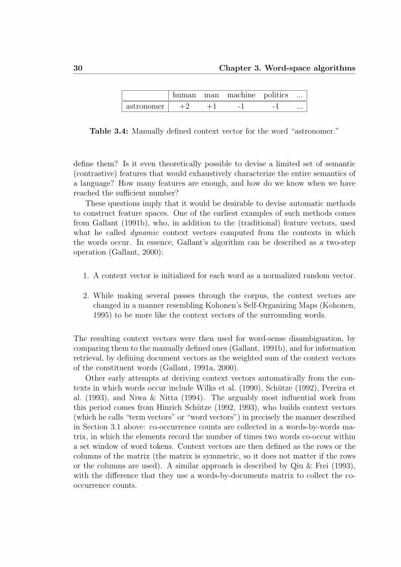
Table 3.4: Manually defined context vector for the word “astronomer.”

define them? Is it even theoretically possible to devise a limited set of semantic(contrastive) features that would exhaustively characterize the entire semantics ofa language? How many features are enough, and how do we know when we havereached the sufficient number?

These questions imply that it would be desirable to devise automatic methodsto construct feature spaces. One of the earliest examples of such methods comesfrom Gallant (1991b), who, in addition to the (traditional) feature vectors, usedwhat he called dynamic context vectors computed from the contexts in whichthe words occur. In essence, Gallant’s algorithm can be described as a two-stepoperation (Gallant, 2000):

1. A context vector is initialized for each word as a normalized random vector.

2. While making several passes through the corpus, the context vectors arechanged in a manner resembling Kohonen’s Self-Organizing Maps (Kohonen,1995) to be more like the context vectors of the surrounding words.

The resulting context vectors were then used for word-sense disambiguation, bycomparing them to the manually defined ones (Gallant, 1991b), and for informationretrieval, by defining document vectors as the weighted sum of the context vectorsof the constituent words (Gallant, 1991a, 2000).

Other early attempts at deriving context vectors automatically from the con-texts in which words occur include Wilks et al. (1990), Schutze (1992), Pereira etal. (1993), and Niwa & Nitta (1994). The arguably most influential work fromthis period comes from Hinrich Schutze (1992, 1993), who builds context vectors(which he calls “term vectors” or “word vectors”) in precisely the manner describedin Section 3.1 above: co-occurrence counts are collected in a words-by-words ma-trix, in which the elements record the number of times two words co-occur withina set window of word tokens. Context vectors are then defined as the rows or thecolumns of the matrix (the matrix is symmetric, so it does not matter if the rowsor the columns are used). A similar approach is described by Qiu & Frei (1993),with the difference that they use a words-by-documents matrix to collect the co-occurrence counts.

3.4. The co-occurrence matrix 31

3.4 The co-occurrence matrix

The approach pioneered by Schutze and Qiu & Frei has become standard practicefor word-space algorithms: data is collected in a matrix of co-occurrence counts,and context vectors are defined as the rows or columns of the matrix. Such amatrix of co-occurrence counts is called a co-occurrence matrix, and is normallydenoted by F (for frequency). As we have already seen, the matrix can either bea words-by-words matrix w × w, where w are the word types in the data, or awords-by-documents matrix w × d, where d are the documents in the data. A cellfij of the co-occurrence matrix records the frequency of occurrence of word i inthe context of word j or in document j. As the attentive reader will have noticed,we have already seen an example of a words-by-words co-occurrence matrix inTable 3.2.

Those versed in the field of information retrieval will recognize words-by-docu-ments matrices as instantiations of the vector-space model developed by GeraldSalton and colleagues in the 1960s within the framework of the SMART information-retrieval system (Salton & McGill, 1983). In the traditional vector-space model, acell fij of matrix F is the weight of term i in document j.4 The weight is usuallycomposed of three components (Robertson & Sparck Jones, 1997):

fij = tfij · dfi · sj

where tfij is some function of the frequency of term i in document j (tf for termfrequency), dfi is some function of the number of documents term i occurs in (df

for document frequency), and sj is some normalizing factor, usually dependent ondocument length (s for scaling).

The point of the first component tfij is to indicate how important term i isfor document j. The idea is that the more often a term occurs in a document, themore likely it is to be important for identifying the document. The observationthat frequency is a viable indicator of the quality of index terms originates in thework of Hans Peter Luhn in the late 1950’s (Luhn, 1958).

The second component dfi indicates how discriminative term i is. The idea isthat terms that occur in few documents are better discriminators than terms thatoccur in many. The arguably most common version of the document frequencymeasure is to use the inverse document frequency (idf), originally established byKaren Sparck Jones (1972), and computed as:

idf = logD

dfi

4Note that I use “term” instead of “word” here. The reason is that multi-word terms areoften used in information retrieval, so it is more natural to speak of “terms” than “words” in thiscontext.


where D is some constant — usually the total number of documents (or a functionthereof) in the document collection.

The third component sj is normally a function of the length of document j,and is based on the idea that a term that occurs the same number of times in ashort and in a long document should be more important for the short one. Thatis, we do not want long documents to end up at the top of the ranking list in aninformation-retrieval system merely because they are long. There are many vari-ations of document-length normalization, ranging from very simple measures thatjust count the number of tokens in a document (Robertson & Sparck Jones, 1997),to more complex ones, such as pivoted document-length normalization (Singhal etal., 1996).

Most information-retrieval systems in use today implement some version ofthis type of combinatorial weight, known as the tfidf family of weighting schemes(Salton & Yang, 1973). This is true also for word-space algorithms that use awords-by-documents co-occurrence matrix. However, word-space algorithms thatuse a words-by-words co-occurrence matrix normally do not use tfidf-weights(the exception being Lavelli et al. (2004), who I will return to in Chapter 15).

Words-by-words co-occurrence matrices are instead typically populated by sim-ple frequency counting: if word i co-occurs 16 times with word j, we enter 16 inthe cell fij in the words-by-words co-occurrence matrix. The co-occurrences arenormally counted within a context window spanning some — usually small —number of words. Remember from Section 3.1 that we used a window consisting ofonly the immediately preceding word and the immediately succeeding word whenpopulating the matrix in Table 3.2.

Note that if we count co-occurrences symmetrically in both directions withinthe window, we will end up with a symmetric words-by-words co-occurrence ma-trix in which the rows equals the columns. However, if we instead count the co-occurrences in only one direction (i.e. the left or right context only), we will end upwith a directional words-by-words co-occurrence matrix. In such a directional co-occurrence matrix, the rows and columns contain co-occurrence counts in differentdirections: if we only count co-occurrences with preceding words within the con-text window, we will end up with a co-occurrence matrix in which the rows containleft-context co-occurrences, and the columns contain right-context co-occurrences;if we only count co-occurrences with succeeding words within the context window,we will end up with the transpose: the rows contain right-context co-occurrences,while the columns contain left-context co-occurrences. We can refer to the formeras a left-directional words-by-words matrix, and to the latter as a right-directionalwords-by-words matrix.

Table 3.5 demonstrates a right-directional words-by-words co-occurrence matrixfor the example data in Section 3.1. Note that the row and column vectors for thewords are different. The row vector contains co-occurrence counts with words

3.5. Similarity in mathematical terms 33

WordCo-occurrents

whereof one cannot speak thereof must be silent

whereof 0 1 0 0 0 0 0 0one 0 0 1 0 0 1 0 0cannot 0 0 0 1 0 0 0 0speak 0 0 0 0 1 0 0 0thereof 0 1 0 0 0 0 0 0must 0 0 0 0 0 0 1 0be 0 0 0 0 0 0 0 1silent 0 0 0 0 0 0 0 0

Table 3.5: Directional words-by-words co-occurrence matrix.

that have occurred to the right of the words, while the column vector containsco-occurrence counts with words that have occurred to their left. I will discuss theuse of context windows more thoroughly in Section 7.4.

3.5 Similarity in mathematical terms

Now that we know how to construct context vectors — we collect data in a co-occurrence matrix and define the rows or columns as context vectors — we mayask what we can use them for? What should we do with the context vectors oncewe have harvested them?

As I mentioned in Section 3.1, an n-dimensional vector effectively identifies alocation in an n-dimensional space. However, the locations by themselves are notparticularly interesting — knowing that the word “massaman” is located at thecoordinates (31, 5,−34, 17,−8,−21, 67) in a real-valued 7-dimensional space doesnot tell us anything (other than its location in the 7-dimensional space, that is).Rather, it is the relative locations that are interesting — knowing that the words“massaman” and “panaeng” are closer to each other than to the word “norrsken”is precisely the kind of information we are interested in. The principal feature ofthe geometric metaphor of meaning is not that meanings can be represented aslocations in a (semantic) space, but rather that similarity between (the meaningof) words can be expressed in spatial terms, as proximity in (high-dimensional)space. As I pointed out in Chapter 2, the meanings-are-locations metaphor iscompletely vacuous without the similarity-is-proximity metaphor.

Now, the context vectors do not only allow us to go from distributional informa-tion to a geometric representation, but they also make it possible for us to compute(distributional, semantic) proximity between words. Thus, the point of the context


vectors is that they allow us to define (distributional, semantic) similarity betweenwords in terms of vector similarity.

There are many ways to compute the similarity between vectors, and the mea-sures can be divided into similarity measures and distance measures. The differenceis that similarity measures produce a high score for similar objects, whereas dis-tance measures produce a low score for the same objects: large similarity equalssmall distance, and conversely. A similarity measure can therefore be seen as theinverse of a distance measure. Generally, we can transform a distance measuredist(x, y) into a similarity measure sim(x, y) by simply computing:

sim(x, y) =1

dist(x, y)

The arguably simplest vector similarity metric is the scalar (or dot) product be-tween two vectors ~x and ~y, computed as:

sims(~x, ~y) = x · y = x1y1 + x2y2 + ... + xnyn

Another simple metric is the Euclidian distance, which is measured as:

diste(~x, ~y) =

√

√

√

√

n∑

i=1

(xi − yi)2

The Euclidean distance is a special case of the general Minkowski metric:

distm(~x, ~y) =

(

n∑

i=1

|xi − yi|N)

1

N

with N = 2. If we let N = 1, we get the City-Block (or Manhattan) metric, andif we let N → ∞, we get the Chebyshev distance. An illustration (inspired byChavez & Navarro (2000)) of the differences between a few Minkowski metrics isgiven in Figure 3.3.

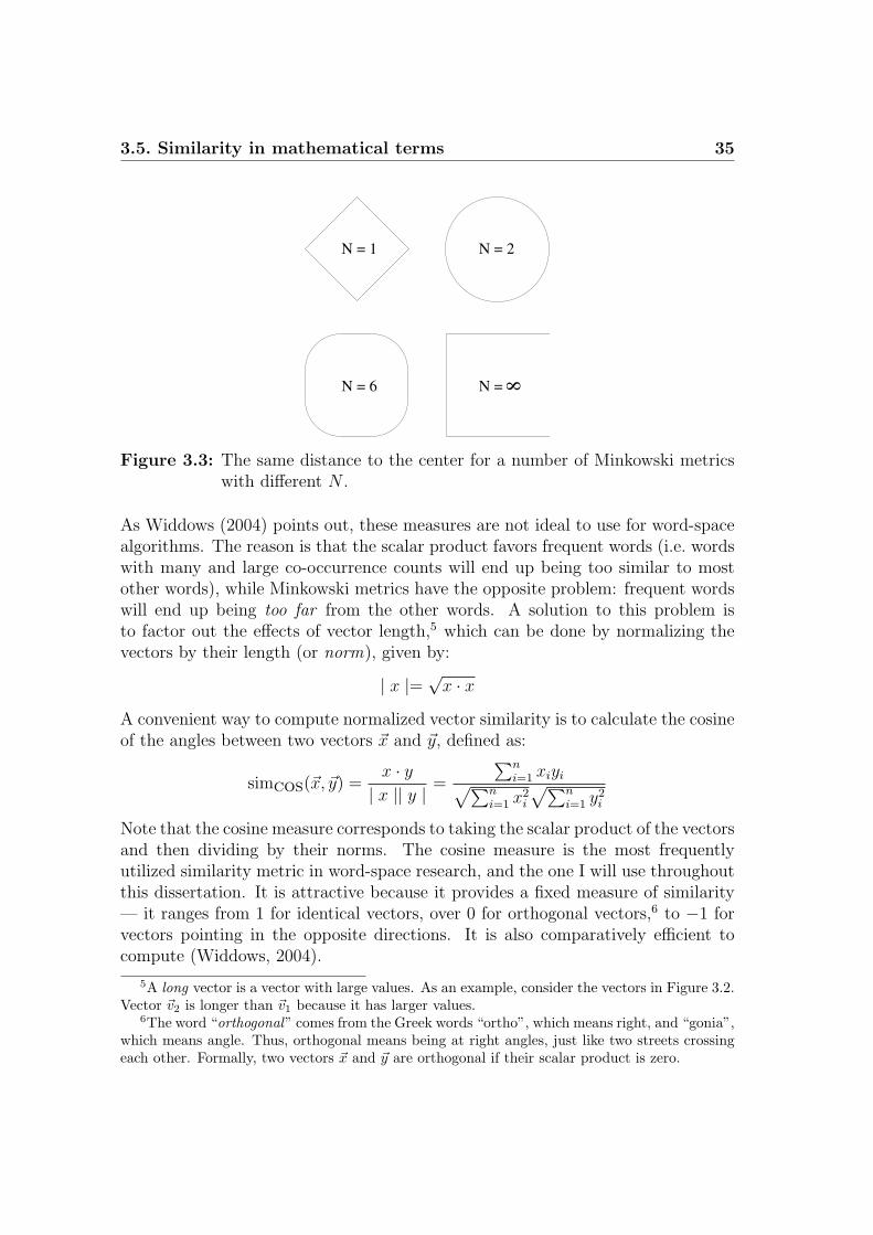
3.5. Similarity in mathematical terms 35

N = 1 N = 2

N = 6 N = 8

Figure 3.3: The same distance to the center for a number of Minkowski metricswith different N .

As Widdows (2004) points out, these measures are not ideal to use for word-spacealgorithms. The reason is that the scalar product favors frequent words (i.e. wordswith many and large co-occurrence counts will end up being too similar to mostother words), while Minkowski metrics have the opposite problem: frequent wordswill end up being too far from the other words. A solution to this problem isto factor out the effects of vector length,5 which can be done by normalizing thevectors by their length (or norm), given by:

| x |=√

x · x

A convenient way to compute normalized vector similarity is to calculate the cosineof the angles between two vectors ~x and ~y, defined as:

simcos(~x, ~y) =x · y

| x || y | =

∑ni=1 xiyi

√∑n

i=1 x2i

√∑n

i=1 y2i

Note that the cosine measure corresponds to taking the scalar product of the vectorsand then dividing by their norms. The cosine measure is the most frequentlyutilized similarity metric in word-space research, and the one I will use throughoutthis dissertation. It is attractive because it provides a fixed measure of similarity— it ranges from 1 for identical vectors, over 0 for orthogonal vectors,6 to −1 forvectors pointing in the opposite directions. It is also comparatively efficient tocompute (Widdows, 2004).

5A long vector is a vector with large values. As an example, consider the vectors in Figure 3.2.Vector ~v2 is longer than ~v1 because it has larger values.

6The word “orthogonal” comes from the Greek words “ortho”, which means right, and “gonia”,which means angle. Thus, orthogonal means being at right angles, just like two streets crossingeach other. Formally, two vectors ~x and ~y are orthogonal if their scalar product is zero.

Chapter 4

Implementing word spaces

“Of course, it’s so simple! Wait, no it’s not. It’s needlessly complicated!”(Homer Simpson in “The Computer Wore Menace Shoes”)

In the last chapter, I built a bridge between the distributional methodology andthe geometric metaphor of meaning. The bridge turned out to be the concept of acontext vector, which allows us to go from distributional statistics to a geometricrepresentation. In this chapter, I will discuss a couple of problems with word-space algorithms, and look at how different implementations of the word-spacemodel handle them.

4.1 The problem of very high dimensionality

When writing an algorithm that implements the word-space model, choosing vec-tor similarity metric is not the only design decision we have to make. Another —important — decision is how to handle the potentially very high dimensionalityof the context vectors. The problem is that the word-space methodology relies onstatistical evidence to construct the word space — if there is not enough data, wewill not have the required statistical foundation to build a model of word distribu-tions. At the same time, the co-occurrence matrix will become prohibitively largefor any reasonably sized data, which seriously affects the scalability and efficiencyof the algorithm. This presents us with the following delicate dilemma: on the onehand, we need as much data as we can get our hands on in order to build a truthfulmodel of language use; on the other hand, we want to use as little data as possiblebecause our algorithms will become computationally prohibitive otherwise.

37

38 Chapter 4. Implementing word spaces

4.2 The problem of data sparseness

Another potential problem with the word-space methodology is that a majority ofthe cells in the co-occurrence matrix will be zero. For all co-occurrence matricesused in the experiments reported in Part III, more than 99% of the entries are zero.This is because only a fraction of the co-occurrence events that are possible in thematrix will actually occur, regardless of the size of the data. Only a tiny amount ofthe words in language are distributionally promiscuous; the vast majority of wordsonly occur in a very limited number of contexts. This phenomenon is well known,and is an example of the general Zipf ’s law (Zipf, 1949).

4.3 Dimensionality reduction

The solution to these predicaments is usually spelled dimensionality reduction. Thepoint of dimensionality reduction here is to represent high-dimensional data in alow-dimensional space, so that both the dimensionality and sparseness of the dataare reduced, while still retaining as much of the original information as possible.In most implementations of word-space algorithms, dimensionality reduction isperformed by first collecting the co-occurrence matrix, and then applying someform of dimensionality-reduction technique to it. The result of such an operationis a much denser and lower-dimensional space, in which the dimensions are typicallyno longer identified with the words or documents in the data.

The arguably simplest form of dimensionality reduction in word-space researchis to filter out words and documents based on either linguistic or statistical criteria.Linguistic criteria can consist of, for example, removing documents based on stylis-tic criteria (Karlgren, 1999), or removing words that belong to certain grammaticalclasses. This latter approach is more widely known as part-of-speech filtering, andnormally consists of removing words that belong to closed grammatical classes,1

since they are assumed to have little or no semantic meaning. An apparent draw-back with part-of-speech filtering is that it only removes a very small fraction ofthe vocabulary; the vast majority of words in language belong to open grammaticalclasses, so the effect of using part-of-speech filtering as dimensionality reduction ismodest at best.

Words can also be filtered out based on statistical criteria, by removing wordswith unfavorable statistical properties. In the simplest case, this means removingwords with very high and very low frequency of occurrence. Note that removing

1Closed grammatical classes are classes that very seldom acquire new members. Examplesinclude adpositions, pronouns, conjunctions, and determiners. Open grammatical classes, on theother hand, are ever-changing, and constantly drop, replace, and add new members. Examplesof such classes are nouns, adjectives, and verbs.

4.4. Latent Semantic Analysis 39

high-frequency words is comparable to using part-of-speech filtering, since wordswith high frequency tend to belong to closed grammatical classes. More sophisti-cated statistical criteria includes the tfidf, and different variants and mixtures ofthe Poisson distribution (Damerau, 1965; Harter, 1975; Katz, 1996).2 While statis-tical filtering typically removes more words than using linguistic criteria, and thusachieves a more distinct dimensionality-reduction effect, it also tends to remove afair amount of words that belong to the open grammatical classes. The problemwith this is that it becomes more or less arbitrary which words are excluded.

4.4 Latent Semantic Analysis

A radically different approach to dimensionality reduction is exemplified by the in-comparably most renowned word-space implementation: Latent Semantic Analysis(LSA) (Landauer & Dumais, 1997). LSA was developed under the name LatentSemantic Indexing (LSI) (Dumais et al., 1988; Deerwester et al., 1990) in the late1980s as an extension to the traditional vector-space model in information retrieval.The terms LSI and LSA have since come to be used more or less synonymously inthe literature, but whereas “LSI” is used primarily in the context of informationretrieval, “LSA” is used for the more general application of these ideas.3 I thususe “LSA” in this dissertation.

The development of LSA was motivated by the inability of the vector-spacemodel to handle synonymy — a query about “boats” will not retrieve documentsabout “ships” in the standard vector-space model. LSA solves this problem byreducing the original high-dimensional vector space into a much smaller space (butstill relatively large; usually a few hundred dimensions), in which the originaldimensions that represented words and documents have been condensed into asmaller set of “latent” dimensions that collapses words and documents with similarcontext vectors. This alleviates the problem with synonymy when retrieval isperformed in the reduced space.

The dimensionality reduction is accomplished by using a statistical dimensional-ity-reduction technique called Singular Value Decomposition (SVD). The mathe-matical details of SVD need not concern us here (but see, for example, Berry et

2The Poisson distribution is a discrete probability distribution that can be used to describethe distributional behavior of function words (i.e. words belonging to the closed grammaticalclasses). Formally, the probability that a function word w will occur exactly k times in a text is

given by Pw(k) = e−λwλk

w

k!where the parameter λw is the average number of occurrences of w

per text: λw = fT

where f is the total number of occurrences of w in the collection, and T is thetotal number of texts in the collection.

3Susan Dumais and Thomas Landauer, personal communication. Apparently, the patent forthe original application of an information-retrieval system based on these ideas refers to it as“LSA.”


al. (1995) for more details); for the present study it is sufficient to note that SVDis a matrix factorization technique that decomposes, or factorizes,4 the originalmatrix into several (three when using SVD) smaller matrices, which can be mul-tiplied to reproduce the original one. These smaller matrices contain the linearlyindependent factors of the original matrix (in the case of SVD, they are called“singular vectors” and “singular values”).5 If the smallest factors are disregardedwhen multiplying the smaller matrices, the result will be an approximation of theoriginal co-occurrence matrix. This process is called truncated SVD, and is thefavored dimensionality-reduction method in LSA.6

The applicability of LSA for information retrieval is well documented (Deer-wester et al., 1990; Dumais, 1993; Dumais et al., 1997; Jiang & Littman, 2000).7

The rationale for using SVD in an information-retrieval setting is obvious: wordswith similar co-occurrence patterns are grouped together, alleviating problems withsynonymy, and allowing for the retrieval of documents that need not contain anyof the query words. However, one may ask what the benefit of using SVD for theword-space model would be (in addition to the purely computational advantagesof dimensionality reduction)?

One of the arguments for using SVD when constructing the word space is thatthe resulting reduced space not only contains “surface” co-occurrence relations(i.e. those contained in the original words-by-documents matrix), but, supposedly,also latent relations that reflect higher-order co-occurrences. Thus, the argumentgoes, when using truncated SVD to restructure the data, the word space will notonly group together words that properly co-occur in a document, but also wordsthat occur in similar contexts (Landauer et al., 1998). The intended effect is thatthe truncated SVD induces relations between rows (or between columns) that aresimilar to the same other rows (or columns) in the original co-occurrence matrix.

4Factorization is a mathematical process where an object is decomposed into the productof other objects, called factors. Thus, a matrix factorization is the right side of the equationF = M1M2 . . .Mm.

5Linear independence means that none of a set of vectors can be written as a linear combi-nation of the other vectors. As an example, the vectors (0,0,1), (0,1,0) and (1,0,0) are linearlyindependent, while the vectors (1,0,0), (0,0,1) and (1,0,1) are not, since the third of these lastvectors can be written as a combination of the other two.

6It is interesting to note that Osgood and colleagues already in 1957 (Osgood et al., 1957) —roughly 30 years before the advent of LSA — mentioned the use of factor analysis to uncoverorthogonal dimensions in the semantic space.

7It should be noted that there are critical voices as well. For example, Isbell & Viola (1998)demonstrate experimentally that truncated SVD generates an approximation that is sub-optimalwith regard to a given information-retrieval problem, and Husbands et al. (2001) observe thatLSA performs sub-optimally on the sizeable TREC collection. Dumais (2004) notes that “thereasons for the inconsistent performance of LSA are not clear and require further research.”Perhaps one of the reasons for this lack of clarity is a dearth of understanding of the semanticproperties of the word-space representations?

4.5. Hyperspace Analogue to Language 41

As an example, if w1 and w2 never occur in the same documents, but sometimesin the same documents as w3, they will get similar vectors after the application oftruncated SVD.

To summarize, LSA uses

• a words-by-documents matrix;

• entropy-based weighting of the co-occurrences, e.g. according to the for-mula (Dumais, 1993):

fij = (log(tfij) + 1) × (1 −(

∑

j

pij log pij

log D

)

)

where D is the total number of documents in the collection, pij =tfij

fiand

fi is the frequency of term i in the whole document collection;

• truncated SVD to reduce and to restructure its dimensionality;

• the cosine measure to compute vector similarities.

4.5 Hyperspace Analogue to Language

An inherently different word-space implementation is the Hyperspace Analogue toLanguage (HAL) (Lund et al., 1995), which, in contrast to LSA, was developedspecifically for word-space research, and was explicitly influenced by Schutze’spaper from 1992.

HAL uses a words-by-words co-occurrence matrix, which is populated by count-ing word co-occurrences within a directional context window 10 words wide. Theco-occurrences are weighted with the distance between the words, so that wordsthat occur next to each other get the highest weight, and words that occur onopposite sides of the context window get the lowest weight. The result of thisoperation is a directional co-occurrence matrix in which the rows and the columnsrepresent co-occurrence counts in different directions. We have already seen anexample of such a directional co-occurrence matrix in Table 3.5 in the previouschapter.

Each row–column pair (i.e. the left and right-context co-occurrences) is thenconcatenated to produce a very-high-dimensional context vector, which has a di-mensionality two times the size of the vocabulary. If such very-high-dimensionalvectors prove to be too costly to handle, HAL reduces their dimensionality by com-puting the variances of the row and column vectors for each word, and discardingthe elements with lowest variance, leaving only the 100 to 200 most variant vec-tor elements. It should be noted that this dimensionality-reduction step is not


essential to HAL; it is only used whenever computational efficiency becomes anissue (Burgess et al., 1998). Thus, HAL uses

• a directional words-by-words matrix;

• distance weighting of the co-occurrences;

• concatenation of row–column pairs;

• if necessary : discarding low-variant dimensions;

• normalization of the vectors to unit length;

• a Minkowski metric to compute vector similarities.

4.6 Random Indexing

Yet another inherently different word-space implementation is Random Indexing(RI) (Kanerva et al., 2000; Karlgren & Sahlgren, 2001; Sahlgren, 2005), which wasdeveloped at the Swedish Institute of Computer Science (SICS) based on PenttiKanerva’s work on sparse distributed memory (Kanerva, 1988). RI is motivatedfirst and foremost by the problem of high dimensionality in other word-space im-plementations. As we have seen, while dimensionality reduction does make theresulting lower-dimensional context vectors easier to compute with, it does notsolve the problem of initially having to collect a potentially huge co-occurrencematrix. Even implementations that use powerful dimensionality reduction, suchas SVD, need to initially collect the words-by-documents or words-by-words co-occurrence matrix. RI targets the problem at its source, and removes the need forthe huge co-occurrence matrix.

Furthermore, RI represents a novel way of conceptualizing the construction ofcontext vectors. Instead of first collecting co-occurrences in a co-occurrence matrixand then extracting context vectors from it, RI incrementally accumulates contextvectors, which can then, if needed, be assembled into a co-occurrence matrix. Thismethodology can be used to assemble both a words-by-documents and a words-by-words co-occurrence matrix. The ability to use both types of contexts is anotherthing that makes RI unique in word-space research.

RI accumulates context vectors in a two-step operation:

1. Each context (i.e. each document or each word type) in the text is assigned aunique and randomly generated representation called an index vector. In RI,these index vectors are sparse, high-dimensional, and ternary, which meansthat their dimensionality r is on the order of thousands, and that they consist

4.6. Random Indexing 43

of a small number (ε) of randomly distributed non-zero elements (as many+1s as –1s). Each word also has an initially empty context vector of thesame dimensionality r as the index vectors.

2. The context vectors are then accumulated by advancing through the textone word token at a time, and adding the context’s (the surrounding wordtypes’ or the current document’s) r-dimensional index vector(s) to the word’sr-dimensional context vector. When the entire data has been processed, ther-dimensional context vectors are effectively the sum of the words’ contexts.

If we then want to construct the equivalent of a co-occurrence matrix, we can simplycollect the r-dimensional context vectors into a matrix of order w × r, where w

(as before) is the number of unique word types, and r is the chosen dimensionalityof the vectors. Note that the dimensions in the RI vectors are randomly chosen,and thus do not represent any kind of context (which is the case in the original co-occurrence matrix) — they constitute a distributed representation. Furthermore,r is chosen to be much smaller than the size of the vocabulary and the number ofdocuments in the data, which means that RI will accumulate (roughly) the sameinformation in the w×r matrix as other word-space implementations collect in thew × w or w × d co-occurrence matrices, but that r � d, w.

The methodology described above can also be used to produce a words-by-words or a words-by-documents co-occurrence matrix by using unary index vectorsof the same dimensionality n as the number of contexts. These unary index vectorshave a single 1 in a different position for each context.8 Mathematically, these n-dimensional unary vectors are orthogonal, whereas the r-dimensional random indexvectors are only nearly orthogonal. This near-orthogonality of the random indexvectors is they key to the RI methodology. Since there are many more nearlyorthogonal than truly orthogonal directions in a high-dimensional space (Kaski,1999), choosing random directions — as we do when generating the index vectors —can get us very close to orthogonality. This means that the r-dimensional randomindex vectors can be seen as approximations of the n-dimensional unary vectors.Consequently, the r-dimensional context vectors produced by RI can be interpretedas approximations, in the sense that their mutual similarities are (nearly) equal,of the n-dimensional context vectors extracted from the co-occurrence matrix.

The near-orthogonality of random directions in high-dimensional spaces is ex-ploited by a number of dimensionality-reduction techniques that includes methodssuch as Random Projection (Papadimitriou et al., 1998), Random Mapping (Kaski,

8As an example, imagine we want to assemble context vectors equivalent to those in a words-by-words co-occurrence matrix. Also imagine we have 1 000 word types in our data. Then thefirst word type would have a 1 000-dimensional index vector with a single 1 in the first position,the second word type would have a single 1 in the second position, and so on.


1999), and Random Indexing. These methods rest on the same insight — theJohnson–Lindenstrauss lemma (Johnson & Lindenstrauss, 1984), which states thatif we project points in a vector space into a randomly selected subspace of suffi-ciently high dimensionality, the distances between the points are approximatelypreserved. Thus, the dimensionality of a given matrix F can be reduced to F ′ bymultiplying it with (or projecting it through) a random matrix R:

F ′

w×r = Fw×dRd×r

Obviously, the choice of the random matrix R is an important design decisionfor dimensionality-reduction techniques that rely on the Johnson–Lindenstrausslemma. As we saw above, if the d random vectors in matrix R are orthogonal, sothat RT R = I, then F ′ = F . If the random vectors are nearly orthogonal, thenF ′ ≈ F in terms of the similarity of their rows. RI uses the following distributionfor the elements of the random index vectors:

rij =

+1 with probability ε/2r

0 with probability r−εr

−1 with probability ε/2r

where r is the dimensionality of the vectors, and ε is the number of non-zeroelements in the random index vectors.

To sum up this section, RI is unique in the following four ways:

1. It is incremental, which means that the context vectors can be used for sim-ilarity computations even after just a few examples have been encountered.By contrast, other word-space implementations, by and large, require the en-tire data to be sampled and represented in the co-occurrence matrix beforesimilarity computations can be performed.

2. It uses fixed dimensionality, which means that new data do not increase thedimensionality of the vectors. Increasing dimensionality can lead to signifi-cant scalability problems in other word-space implementations.

3. It uses implicit dimensionality reduction, since the fixed dimensionality ismuch lower than the number of contexts in the data. This leads to a signifi-cant gain in processing time and memory consumption as compared to word-space implementations that employ computationally expensive dimensional-ity-reduction techniques. As an example, the complexity of computing anSVD is on the order of O(wzd) (under the assumption that the data aresparse), where w is the size of the vocabulary, d is the number of docu-ments, and z is the number of non-zero elements per column (Papadimitriou

4.6. Random Indexing 45

et al., 1998). Performing a random projection of the original (sparse) data —i.e. forming a w× r random matrix and projecting the original w× d matrixthrough it — is O(zrw) (Papadimitriou et al., 1998; Bingham & Mannila,2001), where r is the dimensionality of the vectors. By contrast, producingcontext vectors with RI is only O(wr), since the method is not reliant on theinitial construction of the co-occurrence matrix.

4. It is comparably robust with regards to the choice of parameters. Otherword-space implementations, such as LSA, are very sensitive to the choice ofdimensionality for the reduced space. For RI, the choice of dimensionality is atrade-off between efficiency and performance (random projection techniquesperform better the closer the dimensionality of the vectors is to the number ofcontexts in the data (Kaski, 1999; Bingham & Mannila, 2001)). In previousexperiments, we have shown that the performance of RI reaches a stable levelwhen the dimensionality of the vectors become sufficiently large (Sahlgren &Coster, 2004; Sahlgren & Karlgren, 2005a).

Part II

Setting the scene

47

Chapter 5

Evaluating word spaces

“I typed ’pathetic clown’ into a search engine, and your name popped right up!”(Small girl to Krusty the Clown in “Insane Clown Poppy”)

In the two previous chapters, I explained how to build a word space. I first in-troduced the general word-space algorithms, and the central notion of a contextvector. I then discussed a couple of problems with the word-space methodology,and identified dimensionality reduction as the solution to these problems. I alsoreviewed three inherently different implementations of the word-space model: LSA,HAL and RI.

Now, imagine that we have produced a word space by using any of the imple-mentations described in the previous chapter. How can we determine whether itis a good word space? How can we evaluate it? Do we even know what it is weshould evaluate? The notion of evaluation is the subject matter of this chapter.

5.1 Reliability

As we saw in Chapter 4, a central concern in word-space research is how to gofrom the original context space to a reduced, more compact, representation. Wesaw that dimensionality reduction can be performed in a number of different ways,and that it typically involves a number of parameters that have to be optimized inorder to arrive at a feasible approximation. We also saw that the implementationsdiffer with regards to which weighting scheme, which type of context, and whichsimilarity metric they use. Obviously, each of these factors influence the perfor-mance of the resulting word space, so parameter optimization is a main focus inword-space evaluations. This typically means optimizing the mentioned factorswith regards to the performance of the word space in some specific experiment.

49

50 Chapter 5. Evaluating word spaces

The overall important property of such experiments is reliability, and concernsthe question how consistent the experiment is. Does it produce roughly the sameresult when repeated, or is there a large variation in the results? As an example,consider an IQ test in which a test subject’s results fluctuates between moronicand genius level. Would we say that such a test is useful? Probably not. It isdifficult, if not impossible, to draw any conclusions from comparisons using a testwhose results are inherently inconsistent.

In the following sections, I provide a brief overview over the most commonevaluation schemes in current word-space research. I begin with a somewhat tersepresentation of my own previous experiments (Sections 5.2 through 5.4), beforeturning to a very brief and simplified summary of other evaluations of word spaces(Section 5.5).

5.2 Bilingual lexicon acquisition

In Sahlgren (2004) and Sahlgren & Karlgren (2005a), we used RI to acquire bilin-gual lexica from aligned parallel data. This was done by first assigning one indexvector to each alignment in the parallelized bilingual data. In our experiments,we used document-aligned data. This means that the corresponding documents(i.e. the alignments) in both languages were represented by the same index vector.Context vectors were then produced by adding a document’s index vector to thecontext vector for a word every time the word occurred in that document. Theresult was that if two words in opposite languages occurred in exactly the samealigned documents, their context vectors became identical. By the same token, iftwo words in opposite languages occurred in mostly the same aligned documents,their context vectors became similar.

We could then extract the h most similar words in the opposite language toany word in the data. This was done by computing the similarity between thecontext vector of a given word, and the context vectors of all words in the oppositelanguage. By discarding all but the h words whose context vectors were mostsimilar to that of the given word in the other language, we effectively compiled abilingual lexicon.

We applied this methodology to English–German and Swedish–Spanish paralleldata, and evaluated the resulting bilingual lexica by comparing them to onlinelexical resources. For every word in our data that was also found in the onlinelexical resources, we counted the number of words that were listed as translationsin both the acquired bilingual lexica and in the online lexical resource. Around60% of the translations in the acquired bilingual lexica were also listed in the onlinelexical resources. This result reflected the need for linguistic preprocessing,1 and

1Plausible translations were rejected because of morphological and orthographical variation.

5.3. Query expansion 51

the importance of using topically compatible data and lexica. More than anything,these experiments demonstrated the need for devising more pertinent evaluationmethodologies for word-space research.

5.3 Query expansion

In a number of experiments (Sahlgren & Karlgren, 2002; Sahlgren et al., 2003,2002; Karlgren, Sahlgren, Jarvinen, & Coster, 2005; Karlgren, Sahlgren, & Coster,2005), we have used RI for both monolingual and bilingual query expansion, forbilingual query translation, and for monolingual query-word selection.

Query expansion is the adding of words to a query in order to improve itsrecall or precision (depending on how the added words are used by the retrievalengine). When using word-space methodology for this purpose, we first select anumber of query words. Then, for each query word, we extract the h most similarwords (possibly in another language) from the word space, and add these wordsto the query. When using word-space methodology for query translation, we use abilingual word space produced from parallel data, as described in Section 5.2 above.For each query word, we then we extract only the most similar word in the otherlanguage, and use this as translation. Finally, we use the word-space methodologyfor query-word selection by first selecting a small number of salient query words,and then adding words to the query based on how similar their context vectors areto the context vectors of the selected query words.

We have used word-space methodology in monolingual settings for query ex-pansion in Swedish, French, and Italian (Sahlgren et al., 2003), and also forFrench query word selection (Karlgren, Sahlgren, & Coster, 2005). In bilingual set-tings, we have used word-space methodology for query expansion and query trans-lation using French–English and Swedish–English (Sahlgren & Karlgren, 2002),English–Japanese (Sahlgren et al., 2002), and Swedish–French (Karlgren, Sahlgren,Jarvinen, & Coster, 2005) data. The results have ranged from “reasonably good”(Karlgren, Sahlgren, Jarvinen, & Coster, 2005; Karlgren, Sahlgren, & Coster,2005), over “decidedly mixed” (Sahlgren & Karlgren, 2002; Sahlgren et al., 2003)to “downright catastrophic” (Sahlgren et al., 2002). However, the performancebottleneck has not so much been the word-space methodology, as it has been aneffect of poor linguistic preprocessing and failure to properly tune the baselineretrieval engines.2

The admittedly mixed results in using word spaces for query expansion clearly

2Information-retrieval systems are sensitive to a number of factors, including morphologicalvariation, compounding phenomena, and the scoring function used by the retrieval engine. Insome of the mentioned experiments, we did not handle these factors, and did not optimize thescoring function. Such neglects gravely affect the retrieval performance.


demonstrate that we have yet to understand how to properly utilize the word-spacemethodology in information-access applications. I submit the hypothesis that thisimpasse is due to the fact that we do not (yet) have a clear picture of what kindof semantic information is captured by the word-space model.

5.4 Text categorization

Text categorization is the task of assigning a given text to one or more of a set ofpredefined categories. In Sahlgren & Coster (2004), we used word-space represen-tations — what we called bag-of-concepts (BoC) — to improve the performance ofa Support Vector Machine (SVM) (Vapnik, 1995) classifier.

The idea was to represent documents in the Reuters-21578 test collection, notas the sum of the words in the documents as is normally done, but as the sum of thecontext vectors of the words in the documents. We then used the resulting tfidf-weighted vectors as input to the SVM classifier. The categorization results werecompared to those reached using standard bag-of-words (BoW) representations.3

The results were that the BoW reached a slightly better result than the BoC overall 90 categories (82.77% vs. 82.29%), but the situation was reversed when onlycounting the ten largest categories (88.09% vs. 88.74%). We also demonstrated howthe performance could be improved from 82.77% to 83.91% over all 90 categories,and from 88.74% to 88.99% over the ten largest categories, by combining the BoWand BoC representations.

Although this experiment showed that the performance of an SVM classifiercan be improved by using word-space representations, it is difficult to determinethe reason for this improvement. We would of course like to believe that the reasonis the added semantic content of the BoC representations, but it could just as wellbe a purely statistical effect due to the denser nature of the BoC vectors. Thiskind of experiment simply involves too many factors to allow us to audibly singleout the reason for the impact of the word-space representations.

5.5 Compacting 15 years of research

It would neither make much sense, nor be practically feasible, to review every singleevaluation of word spaces from the last 15 years. Instead, I will summarize the last15 years of word-space evaluation by identifying five main evaluation schemes.4

3Bag-of-words refers to a representation of a text in which all syntactic and grammaticalstructure has been discarded, and only the mere word tokens are retained. Sort of like pouringall the words in a text into a bag, and then shaking it.

4A more thorough survey specifically focused on evaluations and applications of LSA is Du-mais (2004).

5.5. Compacting 15 years of research 53

• Information retrieval (Deerwester et al., 1988, 1990; Gallant, 1991a; Du-mais, 1993; Caid et al., 1995; Schutze & Pedersen, 1995; Dumais et al., 1997;Schutze & Pedersen, 1997; Jiang & Littman, 2000). These tests normallyuse an information-retrieval test collection, and compare the performance ofa search engine using standard bag-of-words representations, and the word-space representations. As I explained in Section 4.4, the idea is that theword-space representations can be used to alleviate problems with synonymyin the retrieval phase.

• Synonym tests (Landauer & Dumais, 1997; Levy et al., 1998; Karlgren& Sahlgren, 2001; Turney, 2001; Rapp, 2003). These tests are normallydesigned as multiple-choice tests, in which the task is to select the synonym toa given word out of a number of provided alternatives. When using the word-space model to solve this task, vector similarities between the context vectorof the alternatives and the context vector of the given word are computed,and the most similar alternative is chosen as synonym. I will discuss thiskind of evaluation scheme thoroughly in Chapter 12.

• Word-sense disambiguation (Gallant, 1991b; Schutze, 1992, 1993, 1998).In these evaluations, disambiguated data is used to build context vectors foreach of the different senses of a word. These “sense vectors” are then usedfor disambiguation by comparing them to “occurrence vectors” producedfor each unique occurrence of an ambiguous word. The sense whose sensevector is most similar to the occurrence vector is chosen as the sense for thatoccurrence.

• Lexical priming data (Lund et al., 1995; Lund & Burgess, 1996; Mc-Donald & Lowe, 1998; Lowe, 2000). The idea here is to compare distancesbetween context vectors in word space to reaction times collected in lexicaldecision tasks. In such tasks, human subjects are asked to decide, as quicklyas possible, whether a given string of letters is a word or not. The decisionis facilitated when the subjects are exposed to a semantically related word(called a prime) before the decision is made. In psychology, lexical primingeffects are seen as evidence for the strength between concepts in human se-mantic memory. In word-space research, a high correlation between distancesin word space and the reaction times is taken to indicate that the word spaceapproximates human semantic memory.

• Knowledge assessment (Wolfe et al., 1998; Rehder et al., 1998). Thegeneral idea when using word spaces for knowledge assessment is to producetext vectors by summing the context vectors of the constituent words, andthen using these text vectors to compute similarity between a “target” text


and a test text on some subject. This general methodology can be used for anumber of knowledge-assessment tasks. For example, student essays can beautomatically graded by comparing them to “gold standard” texts writtenby experts, to capture a student’s level of background knowledge on somesubject, or to match students with appropriate instructional texts.

5.6 Rethinking evaluation: validity

Having reviewed the most common evaluation schemes in word-space research, wecan note that many of them are not so much evaluations as applications of wordspaces. In many of these experiments, it is not primarily the semantic propertiesof the word space that is in focus, but rather the question whether the word spacecan be used for some particular application. Even if parameter optimization isan integral part of such experiments, they do not focus on how the parametersinfluence the semantic properties of the word spaces.

Optimizing the performance of the word-space model with regards to someparticular task is not the focus of interest here. Rather, it is the question whetherthe word-space model constitutes a viable computational model of meaning thatis the focus of interest in this dissertation. In what sense is it meaning we acquireand represent in the word space, and which parameters determine this information?Evaluating whether, and in what way, the word space is a viable model of meaningrequires not only reliable tests, but valid ones.

Validity addresses the question whether the test measures what it is supposedto measure. Again, consider the IQ test: does that test really measure intelligence,or is it something else that we measure when using it? Without venturing into thishighly explosive territory, we can at least maintain that the validity of the IQ testhas been subject to much heated debate.

So how do we measure the semantic proficiency of the word-space model? Howdo we decide if a given word space is a viable representation of meaning? Considerthe evaluation schemes mentioned above: do they measure this? Surely, some ofthem do, to some extent. But none of them licenses the conclusion that a wordspace is a pertinent representation of all aspects of meaning. Of course, it wouldnot make much sense to claim that our tests should measure meaning in general,since we obviously cannot (or at least thus far have successfully avoided to) providea definite answer to the question what meaning is.

The inability (or hesitation) to define “meaning” is the source of the problemwith defining pertinent evaluation methodologies for measuring the semantic pro-ficiency of the word-space model. If we want to measure meaning, we have betterfirst provide a theory of what meaning is, since it is hopelessly futile to try to mea-sure something without knowing what to measure. Note that the distributional

5.6. Rethinking evaluation: validity 55

hypothesis is not a theory of meaning: it is a discovery procedure for excavatingmeaning similarities, and it does not make any ontological commitments about thenature of meaning. What we have is a theory of representation and a theory ofacquisition, but we have no theory of meaning.

The lesson in this chapter is that we should be very cautious with makingclaims about the semantic nature of the word-space representations based solelyon empirical evidence. Unless we can base our claims on a theory of meaning, suchinterpretations require a considerable leap of faith. The point is that there can beno evidence unless there is a case: if we do not have a hypothesis, we have nothingto verify.

Chapter 6

Rethinking the distributionalhypothesis

“This can’t be what it looks like! There’s gotta be some other explanation.”(Bart Simpson in “Bart of Darkness”)

The last chapter concluded that we need a theory of meaning in order to determinewhether the word-space model is a viable computational model of meaning. Now,the distributional hypothesis, as motivated by the works of Zellig Harris, is a strongmethodological claim with a weak semantic foundation. It states that differencesof meaning correlate with differences of distribution, but it neither specifies whatkind of distributional information we should look for, nor what kind of meaningdifferences it mediates. This does not necessarily mean that the use of the distri-butional methodology as discovery procedure in the word-space model is not wellmotivated by Harris’ distributional approach. On the contrary, it is; but if wewant to uncover the nature of the differences, we need to thoroughly understandthe differential view on meaning.

6.1 The origin of differences: Saussure

The differential view on meaning that Harris assumes in his distributional method-ology does not originate in his theories. Rather, it is a consequence of his theo-retical ancestry. Although Harris’ primary source of inspiration was Americanstructuralist Leonard Bloomfield, the origin of the differential view on meaninggoes back even further, to Swiss linguist Ferdinand de Saussure. Saussure (1857–1913) was one of the fathers of modern linguistics, and an important inspiration forthe Bloomfieldian structuralism that developed into the distributional paradigm.

57

58 Chapter 6. Rethinking the distributional hypothesis

Saussure’s posthumously published collection of lecture notes — Cours de linguis-tique generale — is widely regarded as one of the most influential works throughoutthe history of linguistics. It was his ideas that established the structural study oflanguage, and gave rise to the sciences of structuralism and semiotics.

It should be noted that Saussure himself never used the term “structuralism”in the Cours de linguistique generale.1 Saussure-exegesis is complicated by thefact that the primary source of information (the Cours) consists of a collection oflecture notes that have been edited and published posthumously. Attributing aview to the Saussure of the Cours is not the same thing as attributing a view tothe putative theorist behind the actual lectures. I am well aware of this concern.When I speak of Saussure, I speak of the ideas presented in the Cours, and of thestructuralism they gave rise to.

Saussure saw language as a system of signs, where a sign is an inseparabledichotomy between a signifier and a signified. The signifier is an “image acous-tique” (normally translated as “sound image” or “sound pattern”), which shouldbe understood as the psychological impression of the sound, and not as an actualphysical sound. The signified is the psychological concept related to the soundimpression. The dyadic nature of the sign is depicted in Figure 6.1.

Signified

Signifier

Figure 6.1: The Saussurian sign.

The relation between signifier and signified is purely arbitrary, in the sense thatthere is no natural or internal connection between the concept and the soundimpression. As an example, nothing in the sequence /dog/ (or, to prove the point,/hund/ in Swedish, /gou/ in Mandarin, or /zwala/ in Chechen) motivates theconcept of a dog, and vice versa. The arbitrariness of the sign is a very importantprinciple in structuralist theory, since it guarantees that no extralinguistic factorsinfluence the constitution of signs. Without it, structuralism could never succeed.

An unfortunate side effect of the arbitrariness principle is that it makes itseem as if we all could have different concepts associated with different soundimpressions. If nothing in the sequence /dog/ determines what concepts I connectwith it, then there is nothing that guarantees that my concept of a dog is not thesame as your concept of a cat. This is a notorious philosophical nightmare that

1In fact, as Harris (2001) points out, the term “structure” only occurs three times in theCours, and never in a structuralist sense.

6.1. The origin of differences: Saussure 59

would render communication extremely difficult, if not impossible. Saussure hasan ingenious solution to this potential problem.

According to Saussure (1916/1983), the association between signifier and signi-fied can only be established by a linguistic community as a matter of convention:

...the arbitrary nature of the sign enables us to understand more easilywhy it needs social activity to create a linguistic system. (p.157/111)

Even though Saussure saw language as an essentially social phenomenon, he wasnot interested in questions about its social foundation, and about how the associ-ation between signifier and signified gets established by the linguistic community.Such questions, he argued, belong to the field of diachronic linguistics, while hewas mainly concerned with synchronic linguistics.2 Once the connection betweensignifier and signified has been fixed by convention, the sign finds its role withinthe language system. It is then up to the structuralist to describe how the signfunctions within the language system.

The structuralist is only interested in the structure of language (hence the term“structuralism”), and not in the actual use of language. Saussure believed thatthe object of study for linguistics should be the abstract principles of language asa system, referred to as langue (in English “language”), since they are constitutivefor any individual utterance, referred to as parole (in English “speech”). Saussureillustrated the idea using chess as an analogy. Chess is defined by the rules of thegame together with the pieces and the board. Individual moves and actual gamesof chess are only interesting to the participants, and are not essential to (andmay even obscure) the definition of the game. In the same manner, individualutterances are certainly interesting to the language users, but are not essential for(and may even obscure) the description of the language system.

To continue the chess analogy, the individual pieces of the game are identifiedby their functional differences; the king moves one step at a time in any direction,while bishops move diagonally as many steps as desired. Similarly in la langue,signs are identified by their functional differences. Saussure uses the term valeur(in English “value”) to describe the function of a sign. This is arguably the mostimportant concept in structuralist theory, since it is a sign’s valeur that defines itsrole within the language system. Valeurs are defined purely differentially, so thata sign has a valeur only by virtue of being different from the other signs. Such adifferential view on the functional distinctiveness of linguistic elements highlightsthe importance of the system as a whole, since differences (i.e. valeurs) cannotexist in isolation from the system itself. A single isolated sign cannot enter intodifference relations, since there are no other signs to differ from. In this view, thesystem itself becomes an interplay of functional differences:

2Diachronic (or historical) linguistics studies language over a large period of time, while syn-chronic linguistics studies language at a given point in time.

60 Chapter 6. Rethinking the distributional hypothesis

In the language itself, there are only differences. (Saussure, 1916/1983,p.166/118)

6.2 Syntagma and paradigm

The concept of valeur corresponds to the idea of a thoroughly linguistic aspectof meaning. Consider the difference between the French word “mouton” and theEnglish word “sheep.” These words may be said to have the same extralinguistic(i.e. referential) meaning, but they do not have the same valeur, since Englishmakes a distinction between “mutton” and “sheep” that is not available in French.Thus, the functional differences between the signs within la langue is the key tothe idea of linguistic meaning, and Saussure divides these functional differencesinto two kinds: syntagmatic and paradigmatic relations.3

Syntagmatic relations concern positioning, and relate entities that co-occur inthe text; it is a relation in praesentia. This relation is a linear one, and appliesto linguistic entities that occur in sequential combinations. One example is wordsthat occur in a sequence, as in a normal sentence like “I am hungry.” Syntagmaticrelations are combinatorial relations, which means that words that enter into suchrelations can be combined with each other. A syntagm is such an ordered combi-nation of linguistic entities. For example, written words are syntagms of letters,sentences are syntagms of words, and paragraphs are syntagms of sentences.

Paradigmatic relations, on the other hand, concern substitution, and relatesentities that do not co-occur in the text; it is a relation in absentia. Paradigmaticrelations hold between linguistic entities that occur in the same context but notat the same time, like the words “hungry” and “thirsty” in the sentence “I am[hungry|thirsty]”. Paradigmatic relations are substitutional relations, which meansthat linguistic entities have a paradigmatic relation when the choice of one excludesthe choice of another. A paradigm is thus a set of such substitutable entities.

The syntagmatic and paradigmatic relations are usually depicted as orthogonalaxes in a 2-dimensional grid:

3The word “syntagmatic” (French “syntagmatique”) comes from the Greek word “suntag-matikos,” which means arranged, or put in order. The word “paradigmatic” (French “paradig-matique”) comes from the Greek word “paradeigmatikos,” which means serving as a model, fromthe Greek word “paradeigma,” which means example. It should be noted that Saussure himselfnever used the word “paradigmatique.” According to Harris (2001), it was Hjelmslev who coinedthe term paradigmatic relations as a substitute for Saussure’s “rapports associatifs.” I use theterm “paradigmatic” because it is now the accepted term in structuralist theory.

6.3. A Saussurian refinement 61

Paradigmatic relationsSelections: “x or y or...”

Syntagmatic relationsCombinations:“x and y and...”

she buys green painthe eats blue claythey paint red colour

6.3 A Saussurian refinement

The Saussurian notion of valeur as functional difference along the syntagmatic andparadigmatic axes is the origin of the differential view on meaning so prevalentin structuralist theories. Although Harris was arguably more directly influencedby the works of Bloomfield than of Saussure, the latter’s structuralist legacy isfoundational for both Bloomfield’s and Harris’ theories, and the differential viewon meaning is decidedly foundational for the distributional hypothesis. Armed withthis new-found theoretical insight and terminology, we may answer the questionsfrom the beginning of this chapter: what kind of distributional information shouldwe look for, and what kind of meaning differences does it mediate?

A Saussurian refinement of the distributional hypothesis not only clarifies thesemantic pretensions of the word-space model, but it also elucidates the distribu-tional methodology. As we have seen in this chapter, words have a syntagmaticrelation if they co-occur, and a paradigmatic relation if they share neighbors. Thus,we should be able to populate the word-space model with syntagmatic relations ifwe collect information about which words tend to co-occur, and with paradigmaticrelations if we collect information about which words tend to share neighbors. In-stead of talking about unqualified semantic similarities mediated by unspecifieddistributional patterns, we can now state concisely that:

The refined distributional hypothesis: A word-space model accu-mulated from co-occurrence information contains syntagmatic relationsbetween words, while a word-space model accumulated from informationabout shared neighbors contains paradigmatic relations between words.

Chapter 7

Syntagmatic and paradigmaticuses of context

“Each letter is as important as the one that preceded it. Maybe more important!No, as important.”(Homer Simpson in “Homer to the Max”)

In the last chapter, I excavated the origin of the differential view on meaning, andused the structuralist dichotomy of syntagmatic and paradigmatic relations to re-fine the distributional hypothesis. A consequence of the reformulation is that itbecomes clear that the semantic properties of the word space is determined by thechoice of context. This might seem as a trivial statement, but the fact is that veryfew studies have investigated the effects of using different contexts to generate wordspaces. The other word-space parameters, on the other hand, have been meticu-lously scrutinized. Examples include Nakov et al. (2001), who studied the effectsof using different weighting schemes in LSA; Bingham and Mannila (2001), whoinvestigated the effects of using different dimensionality-reduction techniques; andWeeds et al. (2004), who studied the effects of using different similarity measuresfor computing distributional similarity. By contrast, the impact of using differenttypes of context has been severely neglected. The only previous investigation ofthe impact of different contexts on the word-space model that I am aware of is byLavelli et al. (2004), to which I will return in Chapter 15. Out of all the word-spaceparameters, the choice of context is by far the least studied one.

This is highly remarkable for at least two reasons. Firstly, different word-spacealgorithms and implementations use different notions of context to assemble thecontext vectors. As we saw in Chapter 4, LSA uses a words-by-documents matrix,HAL uses a directional words-by-words matrix, and RI can be used to approximateboth of these representations. Despite their different uses of context, most word-space implementations claim to arrive at the same kind of meaning representations.

63

64 Chapter 7. Syntagmatic and paradigmatic uses of context

Secondly, it follows from the theoretical analysis of the foundations of the distribu-tional hypothesis in the last chapter that syntagmatic and paradigmatic relationsbetween words should be discoverable by using co-occurrence information and in-formation about shared neighbors, respectively. Thus, a qualitative comparisonbetween these different uses of context should be able to divulge this difference.

Before an empirical investigation of the difference between using co-occurrencesand shared neighbors for accumulating context vectors can be performed, we needto know more concisely what these different uses of context entail, what theirdifferences are, and how they can be used to build word spaces. Answering thesequestions is the subject matter of this chapter.

7.1 Syntagmatic uses of context

As I explained in the last chapter, a syntagmatic relation holds between words thatco-occur. The prime example of co-occurrence events is collocations, such as “her-metically sealed,” where the first part “hermetically” very seldom occurs withoutthe second part “sealed.” Collocations are probably the most obvious examplesof syntagmatically related words, because the parts of the collocation tend to oc-cur next to each other, without any intervening words. However, syntagmaticallyrelated words can also be defined as words that co-occur within the same textregion, with a (possibly large) number of words between them. In the same senseas “co-occurrence” and “matrix” constitute a syntagmatically related word pair ina number of places throughout this dissertation, we could say that any two wordsin this paragraph (or section, or chapter, or part, or even dissertation) constitutea syntagmatically related word pair.

I will refer to the use of co-occurrence events for building the word space as asyntagmatic use of context. There is at least one parameter that applies to suchsyntagmatic use of context:

1. A syntagmatic use of context can be characterized by the size of the contextregion within which co-occurrences are counted.

7.2 The context region

When constructing context vectors from a syntagmatic use of context, we let then context regions c in the data define the n dimensions of the word space. Thus,a context vector ~v in a syntagmatic word space has the following constitution:

7.2. The context region 65

~v = (c1, c2, ..., cn)

As I pointed out in Section 3.5, this representation does not mean anything invacuo. It is the similarity between two context vectors constructed in this waythat is of the syntagmatic type.

The context region can be anything from a very small sequence of words to anentire text region. In practice, larger text regions are favored by word-space algo-rithms. The reason for this seems to be primarily that the word-space algorithmsthat prefer a syntagmatic use of context, such as LSA, hail from the information-retrieval community, where a document is a natural context of a word. To see why,consider the information-retrieval universe, in which documents and words are twoof the most basic elements. Documents are assumed to represent topical units(and consequently also topical unities), whereas words are seen as topic indicators,whose distribution is governed by a limited number of topics. In the standard typeof information retrieval, this is as far as the metaphor goes, and elements of theuniverse (e.g. queries and documents) are matched based on word overlap, with-out utilizing the topics. In more sophisticated, LSA-type, information retrieval,the topics constitute the fundamental ontology, and all elements in the universe— such as words and documents — can be grouped according to them.1 In thatway, queries and documents can be matched according to their topicality, withoutnecessarily having to share vocabulary. Note that in both types of informationretrieval, documents constitute the natural context of words.

This is a perfectly feasible simplification of textual reality when viewed froman information-retrieval perspective. However, information retrieval is an artificialproblem, and a “document” in the sense of a topical unit–unity is an artificial notionthat hardly exists elsewhere; before the advent of library science, the idea that thecontent of a text could be expressed with a few index terms must have seemedmore or less appalling. In the “real” world, content is something we reason about,associate to, and compare. The uncritical assimilation by word-space algorithms ofthe information-retrieval community’s conception of context is unfortunate, sincethe simplification is uncalled for, and may even be harmful, outside the information-retrieval universe. In the world beyond information-retrieval test collections (whichtend to consist of text types for which the metaphor actually makes sense, such asshort newswire articles or downloaded web pages), text (and, in the big picture,language) is a continuous flow where topics intertwine and overlap. In this complexstructure, finding a correlate to the information-retrieval notion of a “document”is at best an arbitrary choice. As Ruge (1992) notes:

1Proponents of factor-analytic dimensionality-reduction techniques tend to argue that thesetechniques uncover the topics in the form of latent dimensions, or independent or principalcomponents (Bingham, 2003).


Inside of a large context (e.g. a whole document) there are lots of termsnot semantically compatible. In large contexts nearly every term canco-occur with every other; thus this must not mean anything for theirsemantic properties. (p.318)

So what would be a more linguistically justified definition of context in which tocollect syntagmatic information? Perhaps a clause or a sentence, since they seem tobe linguistic universals; clauses and sentences, or at least the functional equivalentto such entities (i.e. some sequence delimited by some kind of delimiter), seem toexist in every language — spoken as well as written or signalled. Thus, it wouldbe possible to argue for its apparent linguistic reality as context. Sentences havebeen used to harvest co-occurrences by, e.g., Rubenstein & Goodenough (1965),Miller & Charles (1991), and Leacock et al. (1996).

Another possibility would be to use a smaller context region consisting of onlya couple of consecutive words, as in the example with collocations. However, a se-rious problem with using such a small context to collect syntagmatic information isthat very few words — basically only collocations — co-occur often within a smallcontext region. In fact, as, e.g., Picard (1999) points out, the majority of termsnever co-occur. The smaller the context regions are that we use to collect syntag-matic information, the poorer the statistical foundation will be, and consequentlythe worse the sparse-data problem will be for the resulting word space.

7.3 Paradigmatic uses of context

Paradigmatically related words are words that do not themselves co-occur, butwhose surrounding words are often the same. One example of such paradigmati-cally related words is different adjectives that modify the same nouns — e.g. “bad”and “good” in “bad news,” “good news.” As with syntagmatically related words,paradigmatic relations need not only consist of words that share the same imme-diately preceding or succeeding neighbor or neighbors. The paradigmatic relationmay just as well be defined as words that share some, or several, of the s precedingor succeeding neighbors.

I will refer to the use of surrounding words for building the word space as aparadigmatic use of context. There are at least three parameters that apply to thecharacterization of such paradigmatic uses of context:

1. The size of the context region within which paradigmatic information is col-lected.

2. The position of the words within the context region.

7.4. The context window 67

3. The direction in which the context region is extended (preceding or succeed-ing neighbors).

7.4 The context window

When constructing context vectors from a paradigmatic use of context, we let then word types w in the data define the n dimensions of the word space. Thus, acontext vector ~v in a paradigmatic word space has the following constitution:

~v = (w1, w2, ..., wn)

Again, this representation is vacuous by itself. It is the similarity between twocontext vectors constructed in this way that is of the paradigmatic type.

The most common way to collect paradigmatic information is to define a contextwindow of some size and extension, within which the information is collected. Asan example, imagine the following two highly imaginary word sequences:

bla bla bla blo bli bli bli

bla bla bla ble bli bli bli

Notice that blo and ble constitute a paradigmatically related word pair in thisexample, and that it would suffice to look at the immediately preceding and suc-ceeding words to establish this — what we call a 1+1-sized context window. Inthe same manner, a 2+2-sized context window would consist of the two precedingand the two succeeding words, and a 5+3-sized window of the five preceding andthe three succeeding words, and so on. Naturally, nothing precludes us from usingan entire sentence (or, for that matter, an entire text) as context window, but— as we will soon see — most researches favor the use of statically-sized contextwindows. I will use the term focus word to refer to the word in the middle ofthe context window (i.e. the word whose context we are currently analyzing). Thecontext window is normally advanced one word at a time until the entire data hasbeen processed — a so-called sliding context window.

As noted in the previous section, we also need to account for the positionof the words within the context windows, since paradigmatically related wordsmay also be defined as words that share some of the s surrounding words. Forexample, imagine that the word bli in the example above could take any of anumber of different modifiers, so that one sequence would be arbitrarily realized asbla blo e bli, and the other as bla ble r bli. In this case, we would like toexclude the arbitrary modifiers from the context windows. One way to accomplishthis is to use a null-weight for that position in the context window, so that theconfiguration for, e.g., a 1+2-sized window would be 1 + 0 1, where 0 means thatthe word is ignored. This would then be realized in the example as:


bla blo e bli -> blo: (bla) + (0 bli)

bla ble r bli -> ble: (bla) + (0 bli)

It is also possible to weight the positions in the context window more finely, insteadof just using binary values. I will discuss a couple of different weighting schemesfor the positions in the context windows in Section 8.5.

The million-euro question regarding context windows is their size: how manywords to the left and to the right should we count? There have been many sugges-tions in the literature. For example, Schutze (1992) uses a window size of 1 000characters, with the argument that a few long words are possibly better than manyshort words, which tend to be high-frequency function words. Yarowsky (1992)uses 100 words, while Gale et al. (1994) uses 50 words to the left and 50 words tothe right, with the argument that this kind of large context is useful for “broadtopic classification.” Schutze (1998) uses a 50-word window, whereas Schutze &Pedersen (1997) uses a context window spanning 40 words. Niwa & Nitta (1994)uses a 10+10-sized window, and as we saw in Chapter 3, the HAL algorithm usesa directional 10-word window. Black et al. (1988) uses narrow windows spanning3–6 words, Church & Hanks (1989) used 5 words, and Dagan et al. (1993) uses awindow spanning 3 words, when ignoring function words.

As we can see, examples of window sizes range from 100 words to just a coupleof words. There is very seldom a theoretical motivation for a particular windowsize. Rather, the context window is often seen as just another experimentallydeterminable parameter. Levy et al. (1998) is a good example of this viewpoint:

These and other technical and practical questions can only be answeredby careful and time-consuming experimentation. (p.4 in the offprint.)

There seems to be some evidence for the feasibility of using a fairly small contextwindow. Kaplan (1955) asked people to identify the sense of a polysemous wordwhen they were shown only the words in its immediate vicinity. They were almostalways able to determine the sense of the word when shown a string of five words— i.e. a 2+2-sized context window. This experiment has been replicated with thesame result by Choueka & Lusignan (1985). Our previous experiments (Karlgren& Sahlgren, 2001) also indicate that a narrow context window is preferable foracquiring semantic information.

Despite these (admittedly somewhat summary) arguments for the feasibilityof narrow context windows, we should heed the cautious words of Miller & Lea-cock (1998):

...we still don’t understand how to extract an adequate contextual rep-resentation from the local context. [...] perhaps we should look atcontext more broadly. (p.156)

7.5. What is the difference? 69

7.5 What is the difference?

For the sake of clarity, I will demonstrate the different uses of context with aconcrete example. Consider the following text:

Was der Fall ist die Tatsache ist das Bestehen von Sachverhalten

Die Welt ist alles was der Fall ist

Das logische Bild der Tatsache ist der Gedanke

Figure 7.1: Example text.

Now imagine that we collect this text into two co-occurrence matrices; one froma syntagmatic use of contexts, collected within the given sentences; one from aparadigmatic use of contexts, also collected within the given sentences. I onlyinclude content words in this example. The result from the co-occurrence countingis displayed in Tables 7.1 and 7.2.

c1 c2 c3

Welt 1 0 0alles 1 0 0Fall 1 1 0Tatsache 0 1 1Bestehen 0 1 0Sachverhelten 0 1 0logische 0 0 1Bild 0 0 1Gedanke 0 0 1

Table 7.1: Words-by-documents co-occurrence matrix.

Obviously, the matrix constructed from a paradigmatic use of context is muchricher in information, which means that it has a more robust statistical founda-tion. Several researchers have noted this difference between the two approaches;Schutze & Pedersen (1997) argue that a paradigmatic use of context (what theycall lexical co-occurrences) is both quantitatively (because it provides a better sta-tistical foundation) and qualitatively (because the fact that two words occur closeto each other is, they argue, likely to be more significant than the fact that they


w1 w2 w3 w4 w5 w6 w7 w8 w9

Welt (w1) 0 1 1 0 0 0 0 0 0alles (w2) 1 0 1 0 0 0 0 0 0Fall (w3) 1 1 0 1 1 1 0 0 0Tatsache (w4) 0 0 1 0 1 1 1 1 1Bestehen (w5) 0 0 1 1 0 1 0 0 0Sachverhelten (w6) 0 0 1 1 1 0 0 0 0logische (w7) 0 0 0 1 0 0 0 1 1Bild (w8) 0 0 0 1 0 0 1 0 1Gedanke (w9) 0 0 0 1 0 0 1 1 0

Table 7.2: Words-by-words co-occurrence matrix.

occur in the same document) better than a syntagmatic use, and Picard (1999) ob-serves that a syntagmatic use of context can only be used for very frequent words,while a paradigmatic use may be applied for all words.

It now becomes obvious why word-space algorithms that prefer a syntagmaticuse of context favor statistical dimensionality-reduction techniques such as SVDthat smooths the original co-occurrence counts. As we saw in Section 4.4, the appli-cation of factor-analytical dimensionality-reduction techniques to the matrix alle-viates the problem with data sparseness. Furthermore, it has the effect of groupingtogether words that do not necessarily co-occur, but that occur in similar contexts— in other words, it approximates paradigmatic relations. This means that SVD,and related dimensionality-reduction techniques, can be viewed as “poor man’s”paradigmatic relations. This is a very useful tactic in information retrieval, wherewe are forced to work with a syntagmatic words-by-documents matrix. However, inword-space research, it seems futile not to use a paradigmatic words-by-words ma-trix, if that is the kind of relations one wants to model. As Schutze (1992) notes, itis unnecessary to apply SVD (or any other related dimensionality-reduction tech-nique) when using paradigmatic contexts, since they are already dense, and ofcourse already contain paradigmatic relations between words.2

2Some researchers, such as Lemaire & Denhiere (2004), claim that only algorithms that useSVD take advantage of higher order co-occurrences, which they define as relations that holdbetween words that do not co-occur, but that occur in similar contexts. As we saw in Section 7.3,this essentially equals paradigmatic relations. Lemaire’s and Denhiere’s claim stems from a lackof theoretical underpinnings, and is not compatible with the analysis in this section.

7.6. And what about linguistics? 71

7.6 And what about linguistics?

Any linguist that is exposed to this discussion will no doubt frown upon the lackof linguistic sophistication in the use of contexts. We are, after all, throwingaway basically everything we know about language when we are simply countingsurface (co-) occurrences. Some word-space paradigms, such as LSA and HAL,are openly agnostic towards linguistics, even though the latter includes at leastthe bare minimum of linguistic knowledge about word order into the directionalco-occurrence matrix by letting the row and column vectors for a word representco-occurrences from the right and left contexts, respectively. However, rememberfrom Chapter 4 that this directional information is thrown away in the final stagesof the algorithm when the row and column vectors are concatenated. The onlyexperiment I am aware of that exploits the directional information in a directionalwords-by-words co-occurrence matrix is Schutze & Pedersen (1993), to which I willreturn in Section 15.6.

Considering the two different uses of context discussed in this chapter, a paradig-matic use of context is arguably more linguistically sophisticated than a syntag-matic use of context, since a context window at least captures some rudimentaryinformation about word order. But why pretend that linguistics never existed —why not use linguistic knowledge explicitly?

There have been a few attempts at using linguistic knowledge when creating theword space. In Karlgren & Sahlgren (2001), we increased the performance of RIon a synonym test by using lemmatized data. We also experimented with addingpart-of-speech tags to the words, thus performing grammatical disambiguation.However, adding part-of-speech information decreased the performance for all sizesof the context window, except when using a minimal 1+1-sized window. Wiemer-Hastings & Zipitria (2001) also noticed a decrease in performance of LSA when theyadded part-of-speech tags to the words, and Widdows (2003) noted that addingpart-of-speech information improves the representation for common nouns, butnot for proper nouns or finite present-tense verbs when enriching the WordNet3

taxonomy. The reason for the decrease in performance is that adding part-of-speechinformation increases the number of unique words in the data, thus aggravatingthe sparse-data problem.

A more sophisticated approach to utilizing linguistic information is Pado &Lapata (2003), who uses syntactically parsed data to build contexts that reflect thedependency relations between the words. Their approach is inspired by the worksof Strzalkowski (1994) and Lin (1997, 1998a, 1998b), who also used parsed data tocompute distributional similarity between words. In Lin’s experiments, words wererepresented by the frequency counts of all their dependency triplets. A dependency

3http://wordnet.princeton.edu/


triplet consists of two words and the grammatical relationship between them ina sentence, such as (have subj I) from the sentence “I have angst.” Similaritybetween words was then defined as (Lin, 1998b):

simlin(w1, w2) =2 × I(G(w1) ∩ G(w2))

I(G(w1)) + I(G(w2))

where Gw is the set of features possessed by w, and I(G) is the amount of informa-tion contained in a set of features G, calculated as −∑g∈G log P (g), where P (g)is the probability of feature g.

Other attempts at using linguistic information for computing distributional sim-ilarity between words include Hindle (1990), who used predicate–argument struc-ture to determine the similarity of nouns; Hearst (1992), who extracted hyponymsby using lexical–syntactic templates; Ruge (1992), who used head–modifier rela-tions for extracting similar words; and Grefenstette (1992a, 1992b, 1993), who alsoused syntactic context to measure similarity between words.

On the downside, such linguistically refined notions of context require a non-negligible amount of preprocessing, and tend to suffer from sparse data (Schutze,1998). Furthermore, empirical evidence for the supremacy of linguistically refinedcontexts are still very scarce. Much more research is needed in order to determinethe viability of, e.g., dependency relations for building word spaces.

Part III

Foreground

73

Chapter 8

Experiment setup

“In fact, I made a graph. I make lots of graphs.”(Lisa Simpson in “Homr”)

The last chapter explained what syntagmatic and paradigmatic uses of context are,what the differences are between them, and how they can be applied to assembleword spaces. Having clarified both the terminology and methodology, we cannow turn to a qualitative empirical comparison between these different uses ofcontexts. This chapter describes the experiment setup: the data, the preprocessing,the transformation and weighting schemes, the word-space implementation, thesoftware, the tests, and the evaluation metrics.

8.1 Data

The primary data I use in these experiments is the Touchstone Applied ScienceAssociates (TASA) corpus,1 which consists of high-school level English texts on anumber of different topics such as language arts, health, economics, science, socialstudies, and business. I use this data for two reasons. The first is that the TASAcorpus is divided into sections spanning approximately 150 words. This meansthat I can use both sentences and sections as context regions for the syntagmaticuses of context. Other corpora, such as the British National Corpus (BNC),2 isnot consistently divided into such topically coherent sections.

The other reason for using the TASA corpus is its convenient size. It is largeenough to provide a sound statistical foundation, but small enough to allow forthe construction of an unreduced word space. For large corpora, such as the BNC,

1Kindly provided by courtesy of Thomas Landauer.2http://www.natcorp.ox.ac.uk/

75

76 Chapter 8. Experiment setup

it is necessary to use dimensionality reduction for most experimental settings. Ido not want to use dimensionality reduction in these experiments, since it mightinterfere with the comparison of the different uses of context. In one experimentwhere there is a limited vocabulary, I also include results from the BNC in orderto demonstrate how the corpus size can effect the results. Details of the corpora(after lemmatization) are given in Table 8.1.

Corpus Size Tokens Types Regions

TASA 56 MB 10 802 187 66 586≈ 150 words≈ 12 words

BNC 527 MB 106 523 151 317 961 ≈ 17 words

Table 8.1: Details of the data sets used in these experiments.

In the remainder of this dissertation, I label the context regions that span approx-imately 150 words large context regions, and the ones that span approximately12–17 words small context regions.

8.2 Preprocessing

I use morphological normalization of the data in these experiments. The main rea-son for doing so is that all the resources (i.e. tests, thesaurus entries, associationnorms) used in the following experiments only include base forms of the words.Also, we have demonstrated in previous experiments that the performance of theword-space model benefits from using morphologically normalized data (Karlgren& Sahlgren, 2001). The reason for this is that morphological normalization re-duces the number of word types in the data, without affecting the number of wordtokens. This at least partially remedies problems with sparse data and improvesthe statistical foundation of the model. To perform morphological normalization, Iuse software from Connexor, a Finnish language-technology company that providesparsers and taggers for several different languages.3

8.3 Frequency thresholding

Since the word-space model is based on statistical evidence of word distributions,it is imperative that the words we examine have a sufficient statistical foundation.Low-frequency words suffer from sparse data and will not have sufficiently reliable

3http://www.connexor.com/

8.4. Transformation of frequency counts 77

statistics to enable distributional analysis. I therefore use frequency thresholdingfor words with frequency less than 50 in the following experiments. I depart slightlyfrom this prescript in two experiments. In Chapter 9, I use a frequency thresholdof 20 instead, and for the synonym test in Chapter 12 that only involves 400words, and therefore is much more efficient to execute, I experiment with differentfrequency thresholds for both low-frequency and high-frequency words.

Frequency thresholding can be done either as a preprocessing step by physicallyremoving the words from the data, or by neglecting the words during processing.I opt for the latter approach, and perform frequency thresholding in the followingmanner: words that occur outside the stipulated frequency range are not assignedan index vector, and if such non-indexed words occur in the context window, theirpositions will have weight 0. This way of doing frequency thresholding blanks outpositions in the window rather than removing them. It is arguable that an evenbetter approach would be to dynamically modify the extension of the context win-dows so that they maintain a constant number of word tokens, while still excludingnon-indexed words. The advantage with the favored approach is that it is muchsimpler and much more efficient.

For tests with a specified vocabulary (like the synonym test in Chapter 12 andthe antonym test in Chapter 13), the frequency threshold does not apply to thecontext vectors for the test words. That is, if a test word has a frequency outsidethe allowed frequency range, it is not assigned an index vector (and thus has noimpact on its neighbors’ context vectors). However, it still receives a context vector,and can thus be included in the test.

8.4 Transformation of frequency counts

Since I want to minimize the risk of distorting the comparison by using an unfavor-able instantiation of any type of context, I use a number of different transformationsof the frequency counts when computing the context vectors. By doing so, I op-timize the performance of the word spaces with regards to the different types ofcontext in each particular task.

I use four different transformations for the syntagmatic uses of context in theseexperiments:

• binary: the elements of the vectors are either 1 or 0, where 1 indicates thatthe word has occurred in the context, and 0 that is has not.

• dampened, computed as log(tf+1): the elements are the logarithms of thefrequency of occurrence of the word in the context.

• tfidf, computed as log(tfidf + 1): the elements are the logarithms of thetfidf-value of the word in the context.


• raw: the elements are the raw frequency of occurrence of the word in thecontext.

These transformations are motivated by their widespread use in information-accessresearch (see Section 3.4). Taking the logarithm of the elements in the contextvectors is done in order to reduce the effect of high values. The idea is that co-occurrence events that only occur once or twice in the data are less important thanco-occurrence events that occur several times, but that it is not important whetherthey occur 500 or 50 000 times. Note that the value is incremented with one beforethe logarithm is computed. This is done in order to avoid zero values, for which alogarithm is not defined. In the remainder of the dissertation, I use the followingnotation for the parameters involved in syntagmatic uses of context:

[S : c ∈ {+,−}, a ∈ {binary,dampened,tfidf,raw}]

where c is the context region (+ for large and − for small), and a is the transfor-mation. As an example [S : +,raw] means a syntagmatic use of a large contextregion, with raw frequencies.

8.5 Weighting of context windows

I use two different weighting schemes for the slots in the context windows for theparadigmatic uses of context:

• Constant weighting over the window.

• Aggressive distance weighting according to the formula 21−l where l is thedistance to the focus word.

There are a number of other possibilities for the distance weights. For example, onecould imagine using linear distance weighting where the weight decreases with someconstant (e.g. 0.1) for every step away from the focus word, or distance weightingaccording to the formula 1

lwhere l is the distance to the focus word. Figure 8.1

shows the effects of these different weights. Since linear weighting and 1l-weighting

is intermediate between constant weighting and aggressive weighting, I only usethe latter weights in the following experiments.

In the remainder of the dissertation, I use the following notation for the pa-rameters involved in paradigmatic uses of context:

[P : s ∈ {n + n, n − n}, b ∈ {const,agg}]

where s is the size of the context window (either the size of one window (e.g. 2+2),the size of several windows (e.g. 3+3,4+4), or the range of several context windows

8.6. Word-space implementation 79

0

0.2

0.4

0.6

0.8

1

1 2 3 4 5 6 7 8 9 10

Wei

ght

Window size

No weightsLinear weights

1/l weightsAggressive weights

Figure 8.1: Different weighting schemes of the context windows

(e.g. 1− 10, which means that all window sizes between 1+1 to 10+10 are used)),and b is the weighting scheme (const for constant weights or agg for aggressive21−l weights). As an example [P : 2 + 2,const] means a paradigmatic use of a2+2-sized context window with constant weights.

8.6 Word-space implementation

I do not use any dimensionality reduction of the context vectors in these experi-ments. The reason, which I already mentioned in Section 8.1 above, is that I donot want any external factors to interfere with the comparison of syntagmatic andparadigmatic uses of context. Thus, I use neither LSA, HAL, nor RI, but the unre-duced context vectors from the words-by-documents and words-by-words matrices.For the TASA corpus, the former vectors are 37 619 (for the large context regions)and 784 819-dimensional (for the small context regions), while the latter are 8217-dimensional (after thresholding low-frequency words). For the BNC corpus,the vectors are 5 794 049 vs. 35 089-dimensional (after frequency thresholding).


8.7 Software

The software used in these experiments is called GSDM (for Guile Sparse Dis-tributed Memory) and was written by Anders Holst at SICS. GSDM is an opensource C-library for Guile,4 designed specifically for the RI methodology. The soft-ware provides a number of basic functions for handling texts, vectors, and matrices.All higher-level programming is done in Guile using the basic GSDM functions.GSDM is available under the GNU GPL license.

8.8 Tests

A number of different tests are used in these experiments. Since the point of theexperiments is to verify the hypothesis that syntagmatic and paradigmatic uses ofcontext generate different semantic models, I have tried to select tests that measurenot only different aspects of linguistic meaning but specifically syntagmatic andparadigmatic relations to different degrees. This has not been an easy task, sincesyntagmatic and paradigmatic relations are not mutually exclusive. Many wordsthat enter into paradigmatic relations can also enter into syntagmatic ones, andconversely. The tests used in these experiments do not provide exact measures ofthese relations.

Most of the following tests use some sort of lexical resource for comparison. Oneproblem with this approach is that freely available lexical resources are scarce, in-coherent, and incomplete. It is always an apparent risk when relying on suchresources that the resulting evaluation becomes as much an evaluation of the re-source itself. We have previously encountered and discussed such problems inSahlgren & Karlgren (2005a) and Sahlgren (2006). Another problem with lexicalresources is that they are typically compiled by humans, who are influenced byextralinguistic factors that are not available to the word-space model. Rememberthat the word-space model only claims to represent linguistic meaning. In a sense,whatever the word-space model uncovers is the truth, since that is what is reallythere in the data. The linguistic information contained within a corpus such asthe TASA does not necessarily have to correspond exactly with general humansemantic knowledge. In fact, we would be greatly surprised if it did.

The question how to evaluate models of meaning provides enough material foran entire dissertation in itself. I do not claim to have any definite answer to thisquestion, and I do not intend for these experiments to provide any definite empiricalevidence. The following experiments should be viewed more as indications of theviability of the hypothesis. The tests that I use are

4http://www.gnu.org/software/guile/guile.html

8.9. Evaluation metrics 81

• direct comparison of the word spaces (Chapter 9);

• thesaurus comparison (Chapter 10);

• association test (Chapter 11);

• synonym test (Chapter 12);

• antonym test (Chapter 13);

• part-of-speech test (Chapter 14).

8.9 Evaluation metrics

The evaluation metrics are somewhat different for the different tests. For the directcomparison, I count overlap between neighborhoods in the word space, as furtherdescribed in the next chapter. For the synonym test, I report results as percentageof correct answers, as described in Chapter 12.

For each of the four remaining tests, I employ two different evaluation metrics,which I call lax(h) and strict(h) settings. The h defines the number of nearestneighbors extracted from the word space. For example, if h = 5, I extract the 5nearest neighbors from the word space to each word included in the test. The laxsetting means looking at whether any of the word-space neighbors are listed inthe resource (i.e. thesaurus, association norm, antonym list or part-of-speech list)used in these experiments, while the strict setting means looking at whether allof the word-space neighbors are listed in the evaluation resource. The results arereported as the percentage of word-space neighbors that are listed in the evaluationresource, defined as:

lax(h) = 100 × # correct neighbors

# test words

strict(h) = 100 × # correct neighbors∑

h

A couple of examples might help clarify these evaluation metrics. Suppose we usethe lax(1) setting, and that we have 10 test words. This means that we extract1 nearest neighbor to each of the 10 test words. If 8 of these neighbors are listedin the resource currently used (say, a thesaurus), we will arrive at 100× 8

10= 80%

correct answers. Note that, if we only extract 1 nearest neighbor to each test word,the lax(1) setting is equivalent to the strict(1) setting.

If we instead use lax(10), we will extract 10 nearest neighbors to each of the10 test words. However, since we use the lax setting, we are only interested in


whether any of these 10 nearest neighbors are listed in the resource. It thus doesnot matter whether all or 5 or only 1 of the 10 neighbors are listed in the resource.Say that for 9 of the test words, we find that at least one of the 10 neighbors (again,we do not care how many) are listed in the resource. We then get 100× 9

10= 90%

correct answers.Contrary to the lax(10) setting, if we instead use a strict(10) setting, we

now count every neighbor that is listed in the resource. In the strict setting itdoes matter whether all or 5 or only 1 of the 10 nearest neighbors are listed inthe resource. Since we have all together 100 neighbors, our maximum result wouldbe 100 × 100

(∑

h)=100= 100%. Say that we only find 26 of all the neighbors in our

resource. We then only get 100 × 26(∑

h)=100= 26% correct answers.

For the thesaurus comparison and the association test, I use lax(1) andstrict(h) evaluation, where h is the number of words listed in the associationnorms and in the thesaurus entries. For the antonym test, which consists of wordpairs, I use lax(10) and strict(1). For the part-of-speech test, which does notinclude a test vocabulary, I use lax(1) and strict(10).

Chapter 9

The overlap between syntagmaticand paradigmatic word spaces

“This is not a clue... or is it?”(Bart Simpson in “Who shot Mr. Burns?)

The first experiment concerning the difference between word spaces produced withsyntagmatic and paradigmatic uses of context is to simply compare the word spaceswith each other. However, since mere ocular inspection of word-space neighbor-hoods is notoriously prone to over-interpretation, it would be useful to define anumeric measurement for the difference between two word spaces.

cut blade

noninimuk

spoonknife

cutterhead

Figure 9.1: Word-space neighborhood produced with [S : +,tfidf]. The circleindicates what the neighborhood would have looked like if a rangearound the word “knife” had been used instead of a constant numberof neighbors (in this case, 6) to define the neighborhood. “Noni” and“Nimuk” are names occurring in the context of knifes.

83

84 Chapter 9. The overlap between word spaces

One way to arrive at a numeric measurement for the difference (or rather thecommonality) between two word spaces is to count the overlap, which I define as thenumber of shared words between neighborhoods in the two spaces. A neighborhoodis simply a region in the word space, centered around a given word. Note thatsuch neighborhoods can be defined in two ways: either as a range around theword (defined by a similarity threshold), or as a number of nearest neighbors. Anexample of a word-space neighborhood is given in Figure 9.1. In the followingexperiments, I opt for the latter approach, and define “word-space neighborhood”as a constant number of nearest neighbors to words in the word spaces.

cut blade

noninimuk

spoonknife

cutterhead

knifespoon

pencil

blanket

hammershovel

hat

A B

Figure 9.2: Overlap between the neighborhoods of “knife” for [S : +,tfidf](space A) and [P : 2 + 2,const] (space B).

Figure 9.2 demonstrates the idea of comparing neighborhoods in two word spaces.The overlap between the spaces is defined as the number of neighbors that occurin both spaces. In the example, only one out of six neighbors (“spoon”) occurs inboth spaces. If there is a large overlap, we can assume that the spaces are verysimilar; if there is a small overlap, we can assume that they are not. Such anadmittedly simple experiment will not tell us in what sense the spaces differ —if at all — but it will tell us whether the hypothesis is worth pursuing or not: Iclearly have to admit defeat if the neighborhoods contain exactly the same words,and the overlap therefore is 100%, since that would indicate that the word spacesare identical.

9.1. Computing the overlap 85

9.1 Computing the overlap

In order to compute the overlap between spaces produced with syntagmatic andparadigmatic uses of context, I first construct word spaces using [S : +,raw](i.e. syntagmatic uses of large context regions with raw frequency counts),[S : −,raw] (i.e. syntagmatic uses of small context regions with raw frequencycounts) and [P : 1 − 20,const] (i.e. paradigmatic uses of context windows rang-ing from 1+1 to 20+20 with constant distance weights). I then select all wordswith frequency above 20 in the TASA corpus, which defines a vocabulary of 13383 words. For each of these words, I extract the 10 nearest neighbors from therespective spaces. I then count how many words occur in both nearest-neighborsets for each of the 13 383 words, thus arriving at a measure of the overlap betweenthe different word spaces.

Context windowOverlap

[S : +,raw] [S : −,raw]10 NNs 1 NN 10 NNs 1 NN

1+1 1.57 1.18 1.74 1.432+2 2.56 1.74 2.93 2.143+3 3.78 2.61 4.19 3.294+4 4.73 3.29 5.13 4.275+5 5.58 4.18 5.95 5.066+6 6.34 5.12 6.34 5.127+7 6.95 5.88 7.18 7.088+8 7.58 6.48 7.74 7.759+9 8.05 7.09 8.08 8.32

10+10 8.50 7.73 8.44 8.8015+15 9.89 9.77 9.31 10.2720+20 10.52 10.74 9.54 10.62

[S : −,raw] 37.45 29.71 – –

Table 9.1: Percentage of nearest neighbors that occur in both syntagmatic andparadigmatic word spaces.

Table 9.1 shows the percentage of mutual nearest neighbors when counting all 10neighbors, and when only counting the closest neighbor in both spaces. The resultsclearly show that there is a very small overlap between the different word spaces.The overlap is fairly small even for syntagmatic spaces produced with differentsizes of the context region; the overlap between [S : +,raw] and [S : −,raw] is37.45% when counting the 10 nearest neighbors, and 29.71% when only counting


the closest one. The overlap between [S : +,raw] and [P : 1 − 10,const], andbetween [S : −,raw] and [P : 1 − 10,const] is of course even smaller, and isbasically the same when counting the 10 nearest neighbors and when only countingthe closest neighbor.

There are three additional noteworthy aspects of these results. The first isthat there is a very small difference in the overlap between paradigmatic wordspaces and syntagmatic spaces produced with large versus small context regions.The largest overlap in these results are between word spaces produced with a widecontext window and a large context region.

The second noteworthy aspect of the results is that the overlap counting the10 nearest neighbors in most cases is a little bit larger than when only countingthe closest neighbor. This might not be surprising considering that there are morepossibilities for overlap in larger neighborhoods than in very small ones. Whatis surprising, however, is that this relationship between the overlap counting 10NNs versus only counting 1 NN is reversed for wider context windows when com-pared to [S : −,raw]. Starting with an 8+8-sized context window, the overlap to[S : −,raw] is larger when only counting the closest neighbor than when countingall 10 nearest neighbors.

The third noteworthy aspect of these results is that the overlap increases withthe size of the context windows. This indicates that wider context windows ap-proximate a syntagmatic use of context. However, consider the difference betweenthe overlap counting the 10 NNs for [S : +,raw] and [S : −,raw], and the over-lap for [S : +,raw] and [P : 20 + 20,const]: 37.45% vs. 10.52%. The overlapis much larger between the two syntagmatic spaces than between a syntagmaticspace and a paradigmatic space produced with a wide context window. In fact,the contexts for [S : −,raw] are only ≈ 12 words, while the context windows for[P : 20+20,const] span 20+20 words, which is almost double the size of the con-text. Thus, the difference between syntagmatic and paradigmatic uses of contextis not primarily a difference of size, but of type; syntagmatic and paradigmatic usesof context yield word spaces with different types of relations between words.

One reason why wider context windows seem to approximate a syntagmatic useof context could be that the wider the context is, the wider is the range of possible(co-) occurrence events. By contrast, a very narrow context harbors a very limitednumber of (co-) occurrence possibilities. The chance that any two words in thedata will share enough of its neighbors to end up close to each other in the wordspace is therefore much greater in a paradigmatic use of wide context windowsthan in a paradigmatic use of narrow ones. Correspondingly, any two words inthe data will co-occur if the context regions in a syntagmatic use of context arelarge enough. Thus, the increasing overlap between syntagmatic uses of contextand paradigmatic uses of wide context windows might be explained by the increasein general (co-) occurrence events when using wide contexts.

9.2. Computing the density 87

9.2 Computing the density

It seems that a paradigmatic use of wide context windows increases the chanceof collecting general occurrence events. This suggests that word spaces assembledfrom such wide windows should be denser than word spaces collected from narrowwindows, simply because there are more occurrence events in the former spaces.A very simple measure of the density of a word space is to compute the averagecosine measure between nearest neighbors in the word space. If the neighbors arevery close to each other, we get a high density measure; if they are distant fromeach other, we get a low score. A high density measure would indicate that thespace is very crowded, which could mean one of two things: either that the spacerests on a solid statistical foundation, or that it is over-crowded and populatedwith chance occurrences.

0.8

0.82

0.84

0.86

0.88

0.9

0.92

0.94

0.96

0.98

1

20+2015+1510+109+98+87+76+65+54+43+32+21+1

Cos

ine

valu

e

Window size

Figure 9.3: Average cosine value between nearest neighbors.

Figure 9.3 shows the results computing such an average density measure for spacesproduced with [P : 1 − 20,const]. As comparison, the average density measurefor spaces produced with [S : +,raw] and [S : −,raw] is 0.23 and 0.08. These lowaverage cosine scores clearly show the sparse-data effect on the density of the word


spaces; the richer the statistical foundation, the denser the word space. The re-markable difference in density between syntagmatic and paradigmatic word spacesfurther demonstrates that collecting paradigmatic relations within wide contextwindows accumulates word spaces that are inherently different from those accumu-lated by syntagmatic uses of context. We have recently suggested that such densitymeasures can serve as indicators of the topical dispersal of a corpus (Sahlgren &Karlgren, 2005b).

9.3 Conclusion

The comparison presented in this chapter suggests that word spaces collected fromsyntagmatic and paradigmatic uses of context are inherently different. Only asmall percentage of the nearest neighbors occur in both syntagmatic and paradig-matic word spaces, regardless of the size of the contexts. These results refute anysuspicion that syntagmatic and paradigmatic word spaces are very similar to eachother. On the contrary, they indicate that these two types of word spaces containinherently different information.

However, it is a legitimate question to ask why there is an overlap at all? Ifwe for a second assume that syntagmatic and paradigmatic word spaces containcompletely distinct relations between words, then should we not expect to see aneven smaller (possibly even non-existent) overlap? As I noted in the previouschapter, syntagmatic and paradigmatic relations are not mutually exclusive, andthese results support this observation. The commonality between syntagmaticand paradigmatic word spaces indicates that some words are both syntagmaticallyand paradigmatically related, and that the difference between syntagmatic andparadigmatic information is not clear-cut.

I conclude this comparison between syntagmatic and paradigmatic word spaceswith the observation that, although a wider context window does lead to a largeroverlap with a syntagmatic use of context, it does not seem possible to reproducea syntagmatic word space by a paradigmatic use of wide context windows. Thismeans that the hypothesis — that syntagmatic and paradigmatic word spacescontain different semantic information — is not only still valid, but supported bythe comparison.

Chapter 10

Thesaurus comparison

“It’s like living in a dictionary!”(Marge Simpson in “I’m Spelling as Fast as I Can”)

It would seem that an obvious way to evaluate word spaces would be to use somekind of repository of semantically related words to compare the word space with.One of the first things that comes to mind for a linguist when talking about se-mantic repositories is thesauri, in which words with similar meanings are listed.Curiously enough, thesauri have not (as far as I am aware) been used to evalu-ate word spaces directly, even though some of the probabilistic approaches that Imentioned briefly in Section 3.2 have used thesauri for evaluation (Grefenstette,1993).

An example of a thesaurus entry for the word “demon” from the thesaurus usedin these experiments (the Moby thesaurus, see below) is displayed in Table 10.1.There are a couple of potential problems with this kind of semantic repository. Thefirst is that thesauri tend to be very wide and include a large number of words.The problem with such lenient repositories of semantic similarity is that they willcontain a fair amount of more or less arbitrary terms. Everyone can probably findat least a couple of unexpected, or even a few far-fetched, terms in the example with“demon” in Table 10.1. It will therefore be very difficult to reproduce a thesaurusentry using word-space neighborhoods even if we have access to vast amounts oftopically pertinent data.

The second potential problem is that there are many different types of semanticrelations represented in this thesaurus entry; among the more obvious ones are(near) synonyms (e.g. “devil,” “satan,” “ghoul,” “monster”), hypernyms (e.g. “evilspirit”), and hyponyms (e.g. “incubus”). Looking at this example, we can findboth syntagmatically and paradigmatically related words. Examples of the formercan be “demon–killer” and “demon–violent,” and examples of the latter can be

89

90 Chapter 10. Thesaurus comparison

demon: baba yaga, lilith, mafioso, satan, young turk, addict, afreet, ape-man,atua, barghest, beast, beldam, berserk, berserker, bomber, brute,bug, cacodemon, collector, daemon, daeva, damned spirits,demonkind, demons, denizens of hell, devil, devil incarnate, dragon,dybbuk, eager beaver, energumen, enthusiast, evil genius, evil spirit,evil spirits, faddist, fanatic, fiend, fiend from hell, fire-eater,firebrand, freak, fury, genie, genius, ghoul, goon, gorilla,great one for, gunsel, gyre, hardnose, harpy, hell-raiser, hellcat,hellhound, hellion, hellish host, hellkite, hobbyist, holy terror, hood,hoodlum, host of hell, hothead, hotspur, hound, incendiary, incubus,infatuate, inhabitants of pandemonium, intelligence, jinni, jinniyeh,killer, lamia, lost souls, mad dog, madcap, monster, mugger, nut,ogre, ogress, powers of darkness, pursuer, rakshasa, rapist,revolutionary, rhapsodist, satan, savage, she-wolf, shedu, souls in hell,specter, spirit, spitfire, succubus, sucker for, supernatural being,termagant, terror, terrorist, the damned, the lost, the undead, tiger,tigress, tough, tough guy, ugly customer, vampire, violent, virago,visionary, vixen, werewolf, wild beast, witch, wolf, yogini, zealot

Table 10.1: Thesaurus entry for “demon.”

“demon–daemon” and “demon–spirit.” This means that it will be difficult to drawany conclusions about the nature of the word spaces based on this comparison.What would it mean if one word space has a particularly high correlation with thethesaurus? Would it mean that it contains more syntagmatic or more paradigmaticrelations? Probably, it would mean that the word space contains a fair amount ofboth types of relations between words. Thus, I hypothesize that the word spacethat correlates the most with the thesaurus contains the widest spectrum of bothsyntagmatic and paradigmatic relations.

10.1 The Moby thesaurus

The Moby thesaurus (second edition) is a freely available lexical resource thatcontains more than 30 000 index words, listed together with more than 2.5 millionsynonyms and related terms.1 There are two main advantages to using the Mobythesaurus. Firstly, it is much more extensive than other freely available thesauri.Secondly, it is distributed in a very simple plain-text format with one entry (i.e. aroot word together with all its related words) per line.

1http://www.dcs.shef.ac.uk/research/ilash/Moby/

10.2. Syntagmatic uses of context 91


Table 10.2 shows the correlation between the Moby thesaurus and word spacesproduced with a syntagmatic use of context. As can be seen in the table, thecorrelation using large context regions is 9.84–10.43%, and the correlation usingsmall context regions is 9.17–9.26%. As can be expected, the correlation is largerfor the lax evaluation, where the figures are 22.35–30.10% vs. 23.93–24.77%. Thisdifference indicates that using large context regions yields somewhat “wider” se-mantic representations that correlate better with the lenient nature of the Mobythesaurus than using small context regions. The reason for this might be that largecontext regions yield word spaces that contain a more diverse blend of both syn-tagmatic and paradigmatic information, while smaller context regions yield wordspaces than contain more specifically syntagmatic relations.

Transformation[S : +] [S : −]

Strict Lax Strict Lax

binary 10.40 29.47 9.26 24.60dampened 10.35 27.77 9.23 24.77tfidf 10.43 30.10 9.17 23.93raw 9.84 22.35 9.17 23.93

Table 10.2: Correlation between thesaurus entries and syntagmatic word spaces.

Note the comparably poor results for [S : +,raw]. This indicates that, eventhough I use the cosine measure of similarity, which effectively normalizes thevectors, there is an over-emphasis of high-frequency words when not dampeningthe frequency counts. Smaller context regions do not have this frequency-inducedproblem, since those co-occurrence events are much more exclusive.


Figure 10.1 shows that there is a very small variation in the results over the differentwindow sizes for the strict evaluation. The results for the windows with constantweights range between 6.97% for [P : 1+1,const] over 7.78% for [P : 3+3,const]to 7.10% for [P : 10 + 10,const]. The best score for the weighted window isalso produced with the 3+3-sized window (7.77%), and the same decreasing trendcan be seen here, albeit not as pronounced, when the size of the window increases(7.71% for [P : 10+10,agg]). The lax evaluation follows the exact same pattern: a3+3-sized window produces the best results for the windows with constant weights(33.81%) and the second best result for the weighted ones (34.20%; [P : 6+6,agg]

92 Chapter 10. Thesaurus comparison

0

10

20

30

40

50

10+109+98+87+76+65+54+43+32+21+1

Per

cent

age

Window size

Constant weights (strict)Constant weights (lax)

Aggressive weights (strict)Aggressive weights (lax)

Figure 10.1: Correlation between thesaurus entries and paradigmatic wordspaces.

is marginally better with 34.21%), and the results decrease as the window sizesincrease. Note that, even though the results for the weighted windows do decreaseas their size increase, the slope is very flat. This indicates that it is only the fewnearest surrounding words that are useful in this particular test. The presence of aslight peak in the results for a window size around 3+3 supports this observation.

10.4 Comparison

We have seen that syntagmatic uses of context yield better results in the strictevaluation (10.43% vs. 7.78%), but that paradigmatic uses of context yield betterresults in the lax evaluation (34.21% vs. 31.10%). Why would such a discrepancyoccur?

I noted above that the Moby thesaurus is very wide, and that it includes afair amount of both syntagmatically and paradigmatically related words. Thefact that syntagmatic uses of context are better than paradigmatic uses in the

10.4. Comparison 93

strict setting indicates that neighborhoods in the syntagmatic word spaces containboth syntagmatically and paradigmatically related words, whereas neighborhoodsin the paradigmatic word spaces might be more homogeneous and mainly containparadigmatic information. If this assumption is true, and syntagmatic uses ofcontext yield more heterogeneous word spaces than paradigmatic uses, there shouldbe a greater chance that semantically unrelated words turn up among the closestneighbors in the syntagmatic word spaces. The fact that paradigmatic uses ofcontext yield better results in the lax evaluation setting supports this observation.

Chapter 11

Association test

“I was just putting words together.”(Homer Simpson in “Old Yeller Belly”)

A semantic repository that is very similar to a thesaurus entry is an associationnorm. It too consists of a list of similar words, with the differences that it typicallycontains fewer words than a thesaurus entry, and that it has been produced byhumans that have been subjected to an association test. An association test isusually designed so that a human subject is presented with a number of words(usually one at a time), and is asked to provide a number of associatively relatedwords to each presented word. The associations provided by the test subjectsare then averaged, and the most frequent associations define the association normfor the particular population to which the test subjects belong. An example ofan association norm for the word “demon” taken from the University of SouthFlorida Free Association Norms is displayed in Table 11.1 (the numbers indicatethe proportion of test subjects that produced the association).

As can be seen in the examples in Table 11.1, these associative relations do notcorrespond to one kind of semantic relation. In the association norm for “demon,”we can find (near) synonyms (“devil,” “satan,” “ghost,” “monster”), a meronym(“wings”), a possible antonym (“deacon”), and a number of adjectival modifiers(“evil,” “possessed,” “bad,” “scary”). This means that we will encounter the sameproblem as the one discussed in relation to thesaurus entries: there are examples ofboth syntagmatically and paradigmatically related words in the association norms.Examples of the former can be “demon–evil” and “demon–scary”, and examplesof the latter can be “demon–devil” and “demon–satan.” However, the associationnorms contain much fewer words than the thesaurus entries and can therefore beexpected to contain fewer arbitrary terms. Furthermore, although the associationnorms do not correlate with linguistic taxonomy, they do represent psychological

95

96 Chapter 11. Association test

demon: devil 0.553evil 0.127satan 0.040ghost 0.033possessed 0.033monster 0.027bad 0.020deacon 0.013scary 0.013wings 0.013

Table 11.1: Association norm for “demon.”

reality — these are, after all, the words that real people deem to be intuitivelyrelated, and so can be assumed to constitute nearest neighbors in the humanassociative space.

Another important consideration when using association norms for compari-son with word-space neighborhoods is that they are inherently sensitive to a largenumber of factors; economic and social status, political and religious conviction,cultural and ethnic background, and linguistic proficiency are all examples of fac-tors that influence what kind of associations people make. To take a currentexample, the word “terrorism” is likely to have entirely different associations foran Islamic fundamentalist than for a conservative American. This presents us witha problem when using association norms to evaluate our word spaces: unless wehave produced the word spaces from pertinent data, we will not be able to matchthe association norm no matter how good a representation of the semantics ofthe data the word space is. Imagine that we build a word space using newswiretext (which is quite common, since many available data collections are based onnews articles), and that we compare it to an association norm collected from apopulation of suburban teens. Chances are we will not see a very large correlationbetween them. However, that does not mean that the word space is flawed — itonly means that it does not reflect the semantics of suburban teens. It may stillconstitute a truthful reflection of the semantics of the newswire texts.

11.1 The USF association norms

I use the freely available University of South Florida Free Association Norms (Nel-son et al., 1998)1 in the following experiments. The norms were collected from

1http://w3.usf.edu/FreeAssociation/


more than 6 000 test subjects who produced responses to 5 019 stimulus words bywriting down the first word they could think of that was meaningfully related, orstrongly associated, to the stimulus word. Such a procedure is called a discrete as-sociation task because each participant is asked to produce only a single associateto each stimulus word.


Table 11.2 demonstrates that the correlation between the association norms andword spaces produced with large text regions is 11.91–13.43%. In contrast tothe thesaurus comparison, the small text regions yield better results in this test:14.93–15.41%. If the analysis in the previous chapter was correct, this should meanthat the association norms are semantically more homogeneous than the thesaurusentries. As can be expected, the correlation increases in the lax evaluation setting,where the figures are 27.88–35.73% using the large regions, and 36.45–37.91% usingthe small ones.

Regarding the frequency transformations, we can note that binary counts pro-duce the best results for the small region but not for the large one, where loga-rithmic transformation of frequencies seems to be a viable alternative. Note againthe inferior results — most pronounced for the large context regions in the laxevaluation setting — using the raw frequency counts.




Table 11.2: Correlation between association norms and syntagmatic word spaces.


As can be seen in Figure 11.1, the correlation between word spaces produced withparadigmatic uses of context and human association norms grows with the size ofthe context windows. The correlation is smallest using [P : 1 + 1,const] (4.17%for the strict evaluation and 12.74% for the lax one), and largest for the strictevaluation using [P : 9 + 9,const] (8.76%) and [P : 10 + 10,agg] (6.05%). The

98 Chapter 11. Association test

best results for the lax evaluation is produced using [P : 8+8, const] (27.95%) and[P : 10 + 10,agg] (18.38%). Regarding weighting of the positions in the contextwindows, we can see that it has a pronounced negative effect on the overlap. Thus,it seems that wider context windows are preferable to use when reproducing humanassociation norms.

0

5

10

15

20

25

30

35

40

10+109+98+87+76+65+54+43+32+21+1

Per

cent

age

Window size



Figure 11.1: Correlation between association norms and paradigmatic wordspaces.

11.4 Comparison

The results from these experiments clearly show that syntagmatic uses of contextproduce word spaces with a much higher degree of correlation to a human asso-ciation norm than word spaces produced with paradigmatic uses of context. Thebest result using paradigmatic word spaces (8.76% for the strict evaluation using[P : 9 + 9,const]) is far surpassed by the best syntagmatic word space (15.41%for the strict evaluation using [S : −,binary]).

11.4. Comparison 99

This could mean one of two things: either that the association norms containmore syntagmatic than paradigmatic information, or that the word spaces pro-duced with syntagmatic uses of context contain a fair amount of paradigmaticinformation. As I argued in the previous chapter, the latter hypothesis is likely tobe correct to a certain extent. However, note that the small context regions out-perform the large ones in this test, while the situation is reversed in the thesauruscomparison. If the assumption in the previous chapter is correct that small contextregions yield word spaces that contain more specifically syntagmatic informationthan the ones produced using large context regions, it is more likely that it is theformer hypothesis that is correct: the association norms contain more syntagmaticthan paradigmatic information. In that case, these results demonstrate that smallcontext regions yield more syntagmatic word spaces than large ones.

Chapter 12

Synonym test

“Inflammable means flammable? What a country!”(Dr. Nick in “Trilogy of Error”)

In contrast to thesauri comparisons and association tests, synonym tests are verycommon in word-space research, no doubt because a synonym test was used forevaluation in the seminal paper by Landauer & Dumais (1997). In this paper,Landauer & Dumais used 80 test items from the synonym part of the standardizedvocabulary test TOEFL (Test Of English as a Foreign Language). The synonympart of this vocabulary test is designed as a multiple-choice test, where the task isto identify the synonym to a given word from four given alternatives. An exampleof a multiple-choice question from the synonym part of the TOEFL is depicted inTable 12.1.

Word Alternatives Synonym

spot sealocation

√

latitudeclimate

Table 12.1: TOEFL synonym test for “spot.”

Execution of a synonym test is easily implemented in a word-space framework.Since it is a multiple-choice test, it is straight-forward to calculate the vectorsimilarity between the context vector for the given word and the context vectorsfor the provided alternatives, and to select the most similar alternative as synonym.This type of test is well-defined and nonparametric (i.e. the test itself involves no

101

102 Chapter 12. Synonym test

parameters), which makes it reliable and easy to use for comparison of differentword-space algorithms, of different parameter settings, and also of different usesof context. In addition to this, most published experiments tend to use the exactsame test set — the 80 multiple-choice TOEFL items that were used by Landauer& Dumais (Landauer & Dumais, 1997; Levy et al., 1998; Karlgren & Sahlgren,2001; Turney, 2001; Rapp, 2003).1

In contrast to the thesaurus comparison and association test, the TOEFL syn-onym test is quite easy. With four alternatives, we can get 25% correct answers bysimply guessing at random. Landauer & Dumais report that foreign applicants toAmerican colleges average 64.5%, but they do not present any average results fornative speakers of English. It seems reasonable to believe that those figures wouldbe significantly higher. We should therefore expect to see much better results inthese experiments than the ones reported in Chapters 10 and 11.

Another difference between the synonym test and the thesaurus and associationtests is that it is perfectly feasible to construct a word space that solves a synonymtest more or less impeccably while still not being a very good model of word mean-ing. The point is that we do not know anything about the actual neighborhoodsin the word space by merely seeing the results from a synonym test, since the testonly utilizes the relative distances between the context vector for the given wordand the context vectors for the alternatives. As an example, consider the followingword space:

spot

the

seven

vasular

sea

ethereal

thermonuclearparrot

climatelatitude

bluelocation

Figure 12.1: Fictive word space.

Now imagine that we use this space to solve the TOEFL item from the exampleabove. Obviously, we would have no problem choosing the correct alternative,but is that fact really significant with regards to determining the quality of thisparticular word space?

On the other hand, whereas the thesaurus entries and association norms in-cluded both syntagmatically and paradigmatically related words, synonyms are

1The 80 TOEFL items were kindly provided by Thomas Landauer.


thoroughly paradigmatic: they are the prime example of paradigmatically relatedwords. Synonyms tend to not co-occur, except in very specific contexts, such as“w1 is the same as w2,” or “w1 means w2.” Rather, synonyms tend to co-occurwith similar other words. As an example, both “bloke” and “lad” tend to occur insimilar contexts, but it is fairly uncommon to see them co-occur. The same appliesto “lift” and “elevator,” or “neighbor” and “neighbour.” Thus, we can expect thatparadigmatic uses of context should yield better results on a synonym test thansyntagmatic uses.

Amongst previously reported experiments using the TOEFL synonym items,we can note that LSA achieved 64.4% (36% without the use of SVD) on a differentcorpus (Landauer & Dumais, 1997). The fact that SVD increases the results inTOEFL experiments with LSA, which implements a syntagmatic use of contexts,further supports the hypothesis from Section 7.5 that the SVD approximates aparadigmatic use of contexts. By contrast, RI managed to reach 72% using the lem-matized TASA corpus and a 3+3 sized distance-weighted context window. Turneyhas reported a score of 73.75% using a probabilistic algorithm called PMI-IR (Tur-ney, 2001), and Levy et al. (1998) reached 76% using the Hellinger distance metric,2

and a small context window with probabilistic weights for the BNC. Rapp (2003)reports an astounding result of 92.5% correct answers, which was produced by ap-plying SVD to a words-by-words matrix collected using a 2+2-sized window over alemmatized and stop-word filtered version of the BNC. Rapp identifies three mainreasons for his fantastic result: the size of his corpus, the preprocessing (lemmati-zation and stop-word filtering), and the use of paradigmatic contexts. To this canbe added the use of SVD to restructure the co-occurrence data. His best resultwithout SVD is 69% correct answers.


Since these experiments use a fixed test vocabulary of 400 words, they can beimplemented in a comparatively efficient manner (it is not necessary to producecontext vectors for all words in the data). I therefore use both the TASA andthe BNC data in these experiments. As discussed in Chapter 8, the BNC doesnot directly allow for the use of large context regions, whereas the TASA can beused with both large and small context regions. The results are summarized inTable 12.2 below.

2The Hellinger metric is given by:

disth(~x, ~y) =∑

(√

x −√y)2


Corpus Transformation [S : +] [S : −]

TASA binary 58.75 51.25TASA dampened 56.25 51.25TASA tfidf 60 52.50TASA raw 53.75 51.25BNC binary N.A. 67.50BNC dampened N.A. 67.50BNC tfidf N.A. 67.50BNC raw N.A. 63.75

Table 12.2: Percentage of correct answers to 80 items in the TOEFL synonymtest for syntagmatic word spaces.

These results follow the same trend as the results in the previous chapters: trans-formation of the frequency counts leads to better results than using the raw oc-currence frequencies. The worst result for both the TASA (using large contextregions) and the BNC (using its small regions) is produced using raw frequencycounts. Regarding the difference between the context regions, Table 12.2 showsthat large context regions produce better results than the small ones for the TASAcorpus. It would have been interesting to see what results a corresponding contextregion could have produced using the BNC data. The difference in the results forthe small and large context regions is consistent with the assumption from theprevious chapters that a smaller context region is more syntagmatic than a largeone, and therefore yields worse result in a thoroughly paradigmatic test.

The best result on the TOEFL synonym test with a syntagmatic use of contextsis 67.50%. This result is reached using the BNC corpus with all tested transfor-mations except the raw frequencies. The best result for the TASA corpus is 60%,using [S : +,tfidf].


The relative efficiency of the synonym test means that I can experiment withdifferent frequency thresholds for the paradigmatic uses of context. I did someinitial experiments varying the low frequency threshold from 1 occurrence to 10with absolutely no effect on the results. By contrast, there is a striking effect whenthresholding high frequency words, as can be seen in Figure 12.2. The parametersfor these experiments are [P : 2 + 2, const].

The best results for the TASA corpus are produced with an upper thresholdof 15 000 or 13 000 occurrences. My version of the lemmatized TASA corpus

12.2. Paradigmatic uses of context 105

60

65

70

75

80

100k50k30k20k19k18k17k16k15k14k13k12k11k10k8k6k

Per

cent

age

Upper frequency threshold

40

45

50

55

60

65

70

75

80

1000k500k200k150k100k75k50k40k30k20k18k16k14k12k10k9k8k7k6k5k

Per

cent

age

Upper frequency threshold

Figure 12.2: Percent correct answers on the TOEFL as a function of upper fre-quency thresholding for paradigmatic word spaces using the TASA(left graph) and the BNC (right graph).

contains 66 586 word types. Thresholding at 15 000 occurrences affects 83 wordtypes (approximately 0.12% of the words), and leaves 66 503. The best results forthe BNC corpus is produced with an upper threshold of 8 000 occurrences. Myversion of the lemmatized BNC data contains 317 961 unique words. Filtering at8 000 occurrences removes some 0.4% of the vocabulary (1 346 word types), andleaves 316 615 unique words.

It is somewhat surprising that the larger of the two corpora requires a lowerfrequency threshold for high-frequency words. One possible reason for this couldbe that the larger data has a wider genre stratification. Our previous experimentsin Sahlgren & Karlgren (2005b), where we applied the density measure introducedin Chapter 9 to (amongst others) the TASA and the BNC corpora, showed acomparatively large difference in word-space density between these two data sets.The BNC received a higher density count than the TASA, which we interpretedas an indication that the BNC is topically more dispersed than the TASA. Suchtopical dispersal leads to “schizophrenic” distributional behavior that distorts thedistributional representations for a larger range of high-frequency words. Thispoints to one of the most serious weaknesses in word-space methodology: it cannotdifferentiate between several simultaneous distributions. When the data is topicallydispersed, word-space representations may become hybrids of different, possiblyunrelated, meanings. In the worst-case scenario, the context vector fails to properlyrepresent any one of the meanings involved.

The results using frequency thresholding demonstrate that thresholding dis-tributionally promiscuous words is beneficial for the word space when solving theTOEFL synonym test. Perhaps, then, upper frequency thresholding could improvethe results using paradigmatic contexts in the other tests? Unfortunately, optimiz-ing the frequency bounds for the other tests is computationally very expensive,


since they involve all words in the data (and not just a small test vocabulary asin the present experiment). I therefore do not use optimized frequency thresholdsin the other experiments. For the TASA corpus, the threshold is set to 15 000occurrences, and for the BNC to 8 000 occurrences.

12.3 Symmetric windows

In these experiments, I study the use of symmetric context windows that have thesame number of window slots on the left and right side of the focus word. The sizeof the context windows range from 1+1 to 10+10. The results are summarized inFigure 12.3.

40

45

50

55

60

65

70

75

80

10+109+98+87+76+65+54+43+32+21+1

Per

cent

age

Window size

Constant weights (TASA)Aggressive weights (TASA)

Constant weights (BNC)Aggressive weights (BNC)

Figure 12.3: Percent correct answers on the TOEFL for paradigmatic wordspaces using the TASA and the BNC.

The results clearly show that narrow context windows spanning only a few wordson each side of the focus word produce the best results. This concurs in theresults reported by Levy et al. (1998). The results decrease for both corpora whenthe windows grow wider. This indicates that a narrow context window is more

12.4. Asymmetric windows 107

paradigmatic than a wide one. The reason for this seems obvious: the furtheraway from the focus word we get, the more possible co-occurrents of the word isthere. Recall from Chapter 9 that paradigmatic word spaces grow denser with thesize of the context windows. This implies that there might be a correlation betweenthe density of a paradigmatic word space and the amount of “noise” (i.e. chanceoccurrence events) it contains. When only looking at the immediately surroundingpositions, there is a very limited set of possible words that could occupy them, andthe resulting word space is consequently less prone to include chance occurrenceevents. In a sense, we could therefore say that the wider the context window,the more noise we get: the denser a paradigmatic word space is, the more chanceoccurrences it contains, and consequently the less paradigmatic it is.

A window spanning two words to the left and two words to the right (i.e. a2+2-sized window) seems to be optimal for the TASA corpus, while a windowspanning three preceding and three succeeding words (i.e. a 3+3-sized window)seems to be optimal for the BNC corpus. This (admittedly small) difference mightbe an artefact of the difference in size between the corpora: the BNC corpus is tentimes larger than the TASA corpus, which means that it provides better statisticalevidence, and therefore facilitates the use of wider context windows. This suggeststhat there might be a correlation between data size and the optimal size of thecontext windows: small data sets require small windows; larger data sets can uselarger windows.

It is somewhat surprising that the smaller TASA corpus generates a better topscore than the ten times larger BNC data (75% vs. 72.50%). At the same time,the results for the BNC are more stable and do not decrease as drastically as theresults for the TASA corpus when the window size increases. This indicates thatmore data makes wider window sizes more viable, but that the quality of the datais the decisive factor for the performance of the word-space model in this particulartest setting.

Regarding the distance-weighting of the context windows, it seems that weight-ing is only beneficial for the outlier positions in larger windows. As can be seen inFigure 12.3, aggressive weights produce the best results for larger windows. Thisis not surprising, since aggressive weighting effectively removes the impact of theoutlier positions, so that the aggressively weighted windows are comparable to the2+2-sized or 3+3-sized windows with constant weights. This further supports theassumption that narrower context windows are more paradigmatic than wide ones.

12.4 Asymmetric windows

It is not obvious a priori that a symmetric window is the best option. It mightjust as well be the case that the left or the right context is more important for


conveying distributional information. Again, since these experiments are efficientto execute, I can examine the effects of using only the left and only the rightcontexts. As with the symmetric windows, I use two different weighting schemesfor the positions within the windows. Figures 12.4 and 12.5 show the results.

40

45

50

55

60

65

70

75

80

10+09+08+07+06+05+04+03+02+01+0

Per

cent

age

Window size



Figure 12.4: Percent correct answers on the TOEFL using only the left contextfor paradigmatic word spaces using the TASA and the BNC.

It is clear that asymmetric windows do not produce as good results as symmetricones. The reason for this could be that asymmetric context windows rely on onlyhalf as much data as symmetric ones. However, the tendencies in the results aresimilar: it is the immediately preceding and succeeding words that are the mostuseful ones. The best result with a left-branching window is a 2+0-sized window(i.e. two words to the left), while the best result with a right-branching window is a0+3-sized window (i.e. three words to the right). Trying a 2+3-sized window onlygenerates 67.5%, which demonstrates that the optimal window size for the left andright contexts might not correspond to the optimal window size when both the leftand right context are taken into account. Again, the results with the asymmetricwindows concur in the observation that a narrow context window seems to be moreparadigmatic than a wide one.

12.5. Comparison 109

40

45

50

55

60

65

70

75

80

0+100+90+80+70+60+50+40+30+20+1

Per

cent

age

Window size



Figure 12.5: Percent correct answers on the TOEFL using only the right contextfor paradigmatic word spaces using the TASA and the BNC.

12.5 Comparison

If we compare the results produced from syntagmatic and paradigmatic uses ofcontext, it is clear that the paradigmatic word spaces produce better results onthe TOEFL synonym test. The best result produced in these experiments is 75%using [P : 2 + 2,const] over the TASA corpus. In comparison, the best re-sult produced from a syntagmatic use of context is 67.5% using the BNC with[S : −,binary,dampened,tfidf]. The fact that the smaller data generates abetter top score for the paradigmatic word space, while larger data generate a bet-ter top score for the syntagmatic word space suggests that context quality is moreimportant for paradigmatic uses of context, while context quantity might be moreimportant for syntagmatic uses of context. These results alone do not warrant suchconclusion, but they do indicate that this phenomenon deserves further study.

Chapter 13

Antonym test

“Ih! I mean: Ah!”(Groundskeeper Willy in “Lard of the Dance”)

Since the last chapter featured a synonym test, it seems appropriate to also in-clude an antonym test in the evaluation of word spaces. Whereas synonyms arewords with the same meaning, antonyms are words with the opposite meaning.Both types of words are substitutable in context, but whereas synonyms retain themeaning of the utterance, antonyms reverse it. As an example, consider how themeaning of the utterance “he looked very alive” is affected when “alive” is sub-stituted with “vital” (a synonym) versus “dead” (an antonym). This means thatantonyms are, just as synonyms, primarily paradigmatically related words, whichoften occur in similar contexts.

However, antonyms have a tendency to become syntagmatic in topical contexts.As I mentioned in the previous chapter, synonyms can also become syntagmatic,but only in very specific contexts. By contrast, if one of the words in an antonymicword pair occurs in a text on a certain topic, it is not uncommon to encounterthe other word as well. As an example, imagine that we talk about the migrationpatterns of a certain kind of fish, say beluga. If the word “deep” occurs in thiscontext, as in “deep waters,” we will probably also encounter the antonym “shal-low,” as in “shallow waters.” We can therefore expect to see good results in thistest not only from paradigmatic word spaces, but also from word spaces built fromlarge context regions.

13.1 The Deese antonyms

In order to test the ability of the word spaces to capture antonymy, I follow theprocedure described by Grefenstette (1992a), who uses a list of antonym pairs

111

112 Chapter 13. Antonym test

taken from work done by Deese (1964). Deese’s original list included 39 antonympairs (see Table 13.1), out of which Grefenstette discarded six pairs because theywere not correctly tagged in his data. I use 38 of the 39 antonym pairs in thefollowing experiments. The pair “single–married” is discarded because the laterword only occurs twice in the TASA.

active–passive dark–light easy–hardbad–good bottom–top happy–sadhigh–low long–short old–young

right–wrong sour–sweet alive–deadbig–little clean–dirty deep–shallow

empty–full hard–soft large–smallnarrow–wide rich–poor rough–smoothstrong–weak back–front black–white

cold–hot dry–wet fast–slowheavy–light left–right new–oldpretty–ugly short–tall thin–thick

alone–together far–near first–lastfew–many single–married inside–outside

Table 13.1: The 39 Deese antonym pairs.


Table 13.2 shows the results from syntagmatic uses of context. As can be seenin the table, the best result for the strict evaluation is produced using a largecontext region (28.95%). At the same time, there is more variation in the resultsfor the large context regions over the different frequency transformations (10.53–28.95%) than for the small context regions (18.42–23.68%). This is true for thelax evaluation as well, where large and small context regions produce the sametop result (47.37%), but where the small context region produces this exact sameresult for all transformations.

Note that the raw frequency counts outperform the other transformations usingboth large and small context regions, and that the difference to the other trans-formations is very large for the large regions. This might be explained by thesyntagmatic tendency of antonyms in topical contexts. Raw frequency counts inlarge context regions seems to capture exactly this kind of topical co-occurrencepatterns.

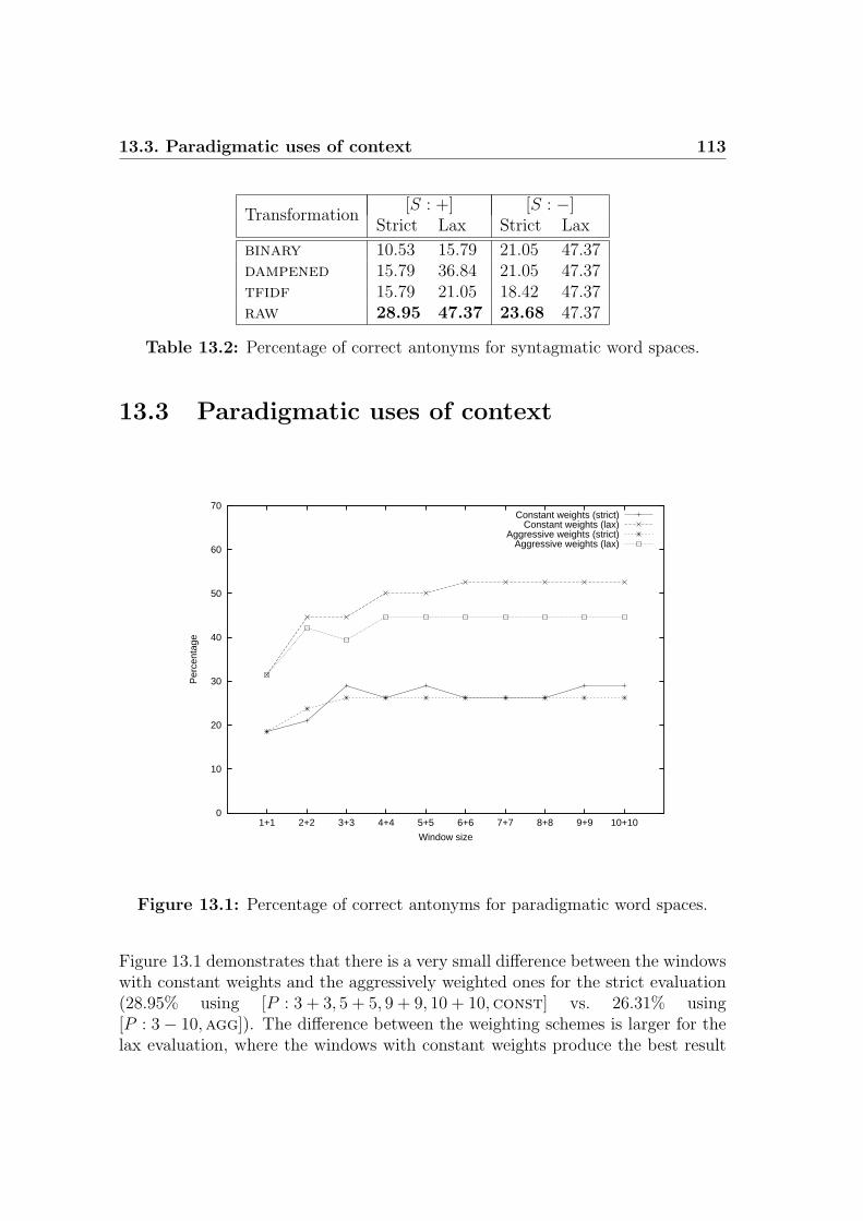
13.3. Paradigmatic uses of context 113




Table 13.2: Percentage of correct antonyms for syntagmatic word spaces.


0

10

20

30

40

50

60

70

10+109+98+87+76+65+54+43+32+21+1

Per

cent

age

Window size



Figure 13.1: Percentage of correct antonyms for paradigmatic word spaces.

Figure 13.1 demonstrates that there is a very small difference between the windowswith constant weights and the aggressively weighted ones for the strict evaluation(28.95% using [P : 3 + 3, 5 + 5, 9 + 9, 10 + 10,const] vs. 26.31% using[P : 3 − 10,agg]). The difference between the weighting schemes is larger for thelax evaluation, where the windows with constant weights produce the best result

114 Chapter 13. Antonym test

(52.63% using [P : 6−10,const] vs. 44.74% using [P : 4−10,agg]). It seems thatwider context windows are preferable in this task. A minimal 1+1-sized windowproduces inferior results for both weights in both evaluations.

13.4 Comparison

Comparing the results produced from syntagmatic and paradigmatic uses of con-text, we can note that the top score for the strict evaluation (28.95%) is producedby both syntagmatic and paradigmatic word spaces. For the lax evaluation, theparadigmatic uses of context windows with constant weights yield better resultsthan the syntagmatic uses of context (52.63% vs. 47.37%). These results supportthe assumption that antonyms become syntagmatic in large contexts (thus thesame top score for paradigmatic uses of context and for syntagmatic uses of largecontext regions in the strict evaluation), but are primarily related through theparadigmatic relation (thus the better results for the paradigmatic word spaces inthe lax evaluation setting).

Chapter 14

Part-of-speech test

“Today we’re going to talk about predicates and predicate nominatives.”“Boring!”(Edna Krabappel and Bart Simpson in “The Parent Rap”)

Rapp (2002) observes that paradigmatic word pairs typically belong to the sameparts of speech, whereas syntagmatic word pairs, although they can belong to thesame parts of speech, typically do not. This observation implies that it shouldbe possible to test whether a word space contains syntagmatic or paradigmaticrelations by looking at how many of the neighbors in the word space have the sameparts of speech. The space that has most neighbors with the same parts of speechcan be assumed to contain the most paradigmatic relations.

In order to test this idea, I select all words in the TASA with frequency above50. I tag the words (n.b. not the data, but only a list of the words) using the freelyavailable TreeTagger,1 and use only the most frequent tag for each word type. Irestrict the tag set to 9 different parts of speech: nouns, verbs, adjectives, adverbs,conjunctions, determiners, pronouns, interjections, and prepositions. I constructword spaces using untagged data, and extract the 10 nearest neighbors to eachword. I then look at how many of the neighbors are listed in the tagged word listwith the same part of speech as the word in question. I define a lax evaluationsetting as only looking at the closest neighbor, and a strict evaluation setting aslooking at all of the 10 nearest neighbors.

Miller & Leacock (1998) argue that the syntactic category of a word can bedetermined by only looking at the words in its immediate environment. An exper-imental result that supports this claim is the success of Eric Brill’s (1994) simplerule-based technique for recognizing syntactic categories without looking further

1http://www.ims.uni-stuttgart.de/projekte/corplex/TreeTagger/

115

116 Chapter 14. Part-of-speech test

than three words preceding or succeeding the focus word. This suggests that anarrow context window should lead to better performance in the part-of-speechtest than using wide windows or context regions.


Table 14.1 shows the results from syntagmatic uses of context. As can be seen inthe table, the small context regions generally lead to better results the large ones.The only exception is the top score for the lax setting, where large regions yield57.79%, while the small ones yield 57.56%. The difference is larger in the strictsetting where small regions outperform the large ones with 53.37% vs. 52.57%.This superiority of the small regions is a tad surprising, given the assumption inthe previous chapters that a small context region is more syntagmatic than a largeone. Under this assumption, we should expect to see less neighbors with the samepart of speech in word spaces produced with small context regions as compared toword spaces produced with large ones. However, I noted above that the part-of-speech test is not very precise, and that syntagmatic neighbors can belong to thesame part of speech.

[S : +] [S : −]Transformation Strict Lax Strict Lax


Table 14.1: Percentage of words with the same part of speech for syntagmaticword spaces.

These results follow the same trend as the other ones with regards to the differ-ences between the frequency transformations for the syntagmatic uses of context.Raw frequency counts are generally inferior, with the sole exception of the strictevaluation setting for the large context regions. Binary counts seem to be the bestchoice in this particular test.


Figure 14.1 shows the results from paradigmatic uses of context. It is obvious thatnarrow context windows yield better results than wide ones in this experiment.

14.3. Comparison 117

Aggressive distance weights clearly outperform the windows with constant weightswhen the window size grows wider, and there is hardly any difference between a3+3-sized and a 10+10-sized aggressively weighted window. The fact that narrowwindows and aggressive distance weighting outperform wide windows with constantweighting further strengthens the observation made in the previous chapters thata narrow context window is more paradigmatic than a wide context window.

50

55

60

65

70

75

80

85

90

10+109+98+87+76+65+54+43+32+21+1

Per

cent

age

Window size



Figure 14.1: Percentage of words with the same part of speech for paradigmaticword spaces.

14.3 Comparison

Comparing the results using syntagmatic and paradigmatic word spaces, it isclear that the paradigmatic space contains more neighbors with the same partof speech than the syntagmatic space. The difference is clearest when using[P : 1 + 1,const] vs. [S : −,binary] (72.94% vs. 53.37% in the strict evaluation,and 76.20% vs. 57.79% in the lax setting). The difference is not as striking whenthe window sizes grow wider (53.39% vs. 53.37% in the strict setting, and 61.10%

118 Chapter 14. Part-of-speech test

vs. 57.79% in the lax setting using [P : 10+10,const] vs. [S : −,binary]). Thus,if Rapp’s suggestion is true that paradigmatic word pairs to a larger extent be-long to the same part of speech than syntagmatic word pairs, these results clearlysupport the hypothesis that looking at shared neighbors captures paradigmaticinformation, while looking at co-occurrences captures syntagmatic information.

Levy et al. (1998) performed a similar experiment where they computed centroidvectors2 for 12 different parts-of-speech by combining the context vectors “from avery large number of different words” belonging to the parts-of-speech. They thenextracted the 100 most frequent words from the 12 different parts-of-speech, andlooked at whether the words’ context vectors were most similar to the centroidvector for the part of speech to which the words belonged. Levy et al. report verygood results for their 12 sets of 100 words, and they observe the same trend thatnarrow context windows yield better performance than wide ones in this kind of“syntactic categorization” task.

2A centroid is the average value, or the center point. A centroid vector is simply the vectorresulting from combining, normally by standard vector addition, a number of vectors.

Chapter 15

Analysis

“Can somebody tell me what the hell is going on here?”(Moe Szyslak in “The Itchy and Scratchy and Poochie show”)

The experiments reported in the previous chapters demonstrate that syntagmaticand paradigmatic word spaces produce consistently different results on a numberof semantic tests. These differences support the hypothesis that syntagmatic andparadigmatic uses of context yield word spaces with inherently different semanticproperties. However, it still remains unclear to what extent the word spaces containsyntagmatic and paradigmatic information, and which parameters influence thisdistinction?

In this chapter, I will further analyze the results reported in the previous chap-ters. Note that the actual performance figures are not very interesting in them-selves; the fact that a word space has an 8.76% correlation with an associationnorm does not tell us very much in itself. I am not interested in producing as goodresults as possible on these tests (and even if I were, it is not obvious how we couldknow if a result is a good result). Rather, I am interested in what the tests can tellus about the semantic properties of the word spaces. Thus, I will first take a closerlook at the effects of the different parameters for syntagmatic and paradigmaticuses of context. Do the parameters influence the semantic properties of the wordspaces, or do they only have statistical effects that optimize a certain representa-tion for a certain test? As should be obvious by now, the parameters do influencethe results in these tests, but that does not necessarily mean that they influencethe syntagmatic and paradigmatic information captured in the word spaces.

After having analyzed the effects of the parameters, I turn to a comparativeanalysis of the performance of the different word spaces. I then conclude theanalysis with a brief review of related research.

119

120 Chapter 15. Analysis

15.1 The context region

Starting with syntagmatic uses of context, I have investigated two parameters forthe production of syntagmatic word spaces: the size of the context regions, andthe transformation of the occurrence counts. Table 15.1 shows the best-performingcontext region for each test and each evaluation metric. Note that it is often thesame region that performs best for a particular test, regardless of which evaluationmetric is used. The exceptions are the antonym test and part-of-speech test (samein the entry for the lax setting in the antonym test means that large and smallregions produce the same top score).

Test Strict Lax

Thesaurus large largeAssociation small smallSynonym largeAntonym large same

PoS small large

Table 15.1: The best context regions for syntagmatic uses of context.

For four out of five tests, large regions produce the best result. This may beexplained by the observation that using large regions provides a better statisticalfoundation than using small ones. Recall from Chapter 9 that the density measurefor a word space produced with [S : +] was 0.23, while it was only 0.08 for a wordspace produced with [S : −]. This difference is a clear indication of the statisticalcontrast between context regions of different sizes.

It is only for the association test and in the strict setting for the part-of-speechtest that small context regions outperform the large ones. Considering the statis-tical incongruity just mentioned, this is an important result. Since the associationtest is the only test that primarily measures syntagmatic relations, while the othertests are primarily paradigmatic, this result strongly indicates that using small— more linguistically motivated — context regions yields more syntagmatic wordspaces than using large ones.

I admit, however, that the discrepancy in the part-of-speech test is baffling. Apossible reason is that this test is a thoroughly paradigmatic test, and thus cannotbe expected to give precise measures of syntagmatic information.

15.2. Frequency transformations 121

15.2 Frequency transformations

Table 15.2 summarizes the best frequency transformations for the syntagmaticuses of context. As with the context regions, the best transformations are moreor less consistent across the evaluation metrics. The exceptions are small contextregions for the thesaurus comparison, large regions for the association test, andlarge regions for the part-of-speech test. For the thesaurus test with small con-text regions, binary counts produce the best result for the strict evaluation, butdampened frequency transformation produce the best result for the lax one; forthe association test with large context regions, dampened frequency transforma-tion produce the best result for the strict evaluation, but tfidf-transformationproduce the best score for the lax setting; for the part-of-speech test with largecontext regions, dampened frequency transformation produce the best results forthe strict evaluation, while binary counts lead to better results for the lax setting.

Test[S : +] [S : −]


Thesaurus tfidf tfidf binary dampened

Association dampened tfidf binary binary

Synonym tfidf tfidf

Antonym raw raw raw allPoS dampened binary binary binary

Table 15.2: The best frequency transformations for syntagmatic uses of context.

Note that binary counts tend to produce good results for the small regions, whereastfidf-transformations produce good results for the large context regions. Thismight not be all too surprising, considering the statistical differences between thedifferent context regions. The binary counts used in these experiments use a singleoccurrence as cut-off point. It is arguable that this is sufficient for small contextregions, but that one should use a higher cut-off point for large regions. The ideais that a single occurrence of a word in a large context region can be duly treatedas a chance occurrence, and thus need not be taken into account (Katz, 1996).Instead, occurrences collected over large context regions can be discriminated bythe use of a df-related transformation. Such transformations have less effects whenthe context regions are many and small, since most words will occur in very fewof these contexts. Finally, the superiority of raw frequency counts in the antonymtest was explained in Chapter 13. To this can be added that the raw frequencycounts performed substandard in all other tests.1

1Very few — if any — real-world systems use raw frequency-counting.


15.3 The context window

I have also used two basic parameters for the paradigmatic uses of context: thesize of the context windows, and the weighting scheme for the positions in thewindows. Table 15.3 demonstrates which window sizes produced the best resultsfor each test and evaluation metric. It is evident that different window sizes areoptimal for different tests; narrow windows spanning only a few surrounding wordsseem optimal for the thesaurus comparison, the synonym test, and the part-of-speech test, while wider windows seem optimal for the association and antonymtests. The optimal window size is consistent over the evaluation metrics.

Test Strict Lax

Thesaurus narrow narrowAssociation wide wideSynonym narrowAntonym wide wide

PoS narrow narrow

Table 15.3: The best window sizes for paradigmatic uses of context.

It is interesting to note that narrow context windows yield better results thanwide windows in both the synonym and part-of-speech tests, which are the mostparadigmatic tests in these experiments. In the association test, on the contrary,wide windows prove to be better. This indicates that word spaces produced froma paradigmatic use of contexts become paradigmatically more refined when usingnarrow context windows. It should be noted that a minimal 1+1-sized windowonly yields the best result for paradigmatic uses of context in the part-of-speechtest. This indicates that the immediate context of a word, which tends to consistsof words from closed grammatical classes, is viable for determining the syntacticcategory of a word, but not as good as the immediately surrounding content wordsfor inferring (semantic) paradigmatic relations between words. A 2+2 or 3+3-sizedwindow seems more viable for that purpose.

15.4 Window weights

Table 15.4 demonstrates that weighting of the positions in the context windowsis suboptimal for every test except the part-of-speech test, and the lax settingin the thesaurus comparison. In the latter test, constant weighting produces thebest result for the strict evaluation (7.78%), but the difference to the top scoreusing aggressive weights (7.77%) is minute. For the part-of-speech test, aggressive

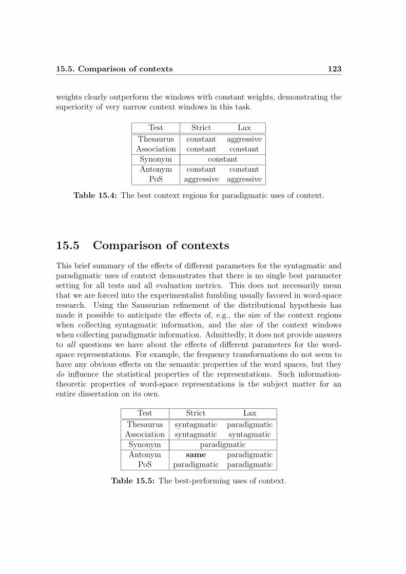
15.5. Comparison of contexts 123

weights clearly outperform the windows with constant weights, demonstrating thesuperiority of very narrow context windows in this task.

Test Strict Lax

Thesaurus constant aggressiveAssociation constant constantSynonym constantAntonym constant constant

PoS aggressive aggressive

Table 15.4: The best context regions for paradigmatic uses of context.

15.5 Comparison of contexts

This brief summary of the effects of different parameters for the syntagmatic andparadigmatic uses of context demonstrates that there is no single best parametersetting for all tests and all evaluation metrics. This does not necessarily meanthat we are forced into the experimentalist fumbling usually favored in word-spaceresearch. Using the Saussurian refinement of the distributional hypothesis hasmade it possible to anticipate the effects of, e.g., the size of the context regionswhen collecting syntagmatic information, and the size of the context windowswhen collecting paradigmatic information. Admittedly, it does not provide answersto all questions we have about the effects of different parameters for the word-space representations. For example, the frequency transformations do not seem tohave any obvious effects on the semantic properties of the word spaces, but theydo influence the statistical properties of the representations. Such information-theoretic properties of word-space representations is the subject matter for anentire dissertation on its own.

Test Strict Lax

Thesaurus syntagmatic paradigmaticAssociation syntagmatic syntagmaticSynonym paradigmaticAntonym same paradigmatic

PoS paradigmatic paradigmatic

Table 15.5: The best-performing uses of context.


Turning now to the arguably central aspect of the experiments: the comparisonbetween syntagmatic and paradigmatic uses of context. Table 15.5 summarizesthe best-performing context type for each test and each evaluation setting. Notethat syntagmatic and paradigmatic uses of context are optimal for different tests:syntagmatic uses of context clearly outperform the paradigmatic uses in the asso-ciation test, but the situation is reversed for the synonym and part-of-speech tests.The difference is not as clear-cut in the thesaurus comparison and the antonymtest, where paradigmatic uses of context outperform the syntagmatic uses in thelax evaluation setting, but not in the strict setting (same in the table means theyproduce the same top score). The fact that certain tests show a greater distinc-tion between syntagmatic and paradigmatic word spaces is a good indicator of theextent to which a certain representation contains syntagmatic versus paradigmaticinformation.

The synonym and part-of-speech tests are clearly paradigmatic tests, while theassociation test is more syntagmatic. The antonym test is more paradigmatic thansyntagmatic, but as I argued in Chapter 13, certain antonyms have a tendencyto become syntagmatic in large contexts, which could explain the viability of thesyntagmatic use of context in this particular test. The thesaurus comparison isthe least precise test in these experiments, and it involves a considerable amountof both syntagmatic and paradigmatic information. This is clearly reflected in theresults.

Table 15.6 summarizes the tests used in this dissertation, the semantic relationsthey primarily measure, the degree to which the relations are essential to the test(− and +), and the use of context that yields the best results in the strict evaluationsettings.

Test Relation Context

Thesaurus comparison both (−) large regionAssociation test syntagmatic (+) small regionSynonym test paradigmatic (+) narrow windowAntonym test paradigmatic (−) wide window

Part-of-speech test paradigmatic (+) narrow window

Table 15.6: The tests used in this dissertation, the semantic relation they pri-marily measure, and the best-performing context.

I conclude this comparative analysis of the results from the experiments reportedin the previous chapters with the observation that distributional information col-lected from co-occurrences in context regions seems to yield syntagmatic represen-tations that are more refined when the regions are smaller, while distributional

15.6. Related research 125

information collected based on the neighboring words seems to yield paradigmaticrepresentations that are more refined the smaller the context windows are.

15.6 Related research

The current investigation is not the first attempt to analyze word spaces in terms ofsyntagmatic and paradigmatic relations. Schutze & Pedersen (1993) compute syn-tagmatic and paradigmatic relations between words by using a directional words-by-words matrix similar to that used in HAL, which they transform using SVD. Byusing a directional matrix and SVD, they produce dimensionality-reduced vectorsfor both the left and right contexts of a word. The idea is then that paradigmaticsimilarity can be computed by comparing the left or the right context vectors,and that syntagmatic similarity can be computed by comparing the left and theright context vectors. The authors provide some examples of syntagmatic andparadigmatic pairs thus extracted but do not make any systematic evaluation ofthe approach, or of the differences between the vectors.

Rapp (2002) experiments with techniques to extract paradigmatic and syntag-matic relations between words. He uses narrow context windows for the paradig-matic relations, and a log-likelihood ratio to extract word pairs whose co-occurrenceis significantly higher than chance for the syntagmatic relations. Rapp points outthat using this kind of probabilistic approach for computing syntagmatic relationsis far more efficient than using the word-space model. As evaluation of the ex-tracted relations, he uses the TOEFL synonym test for the paradigmatic relations,and an association test (the Edinburgh Associative Thesaurus) for the syntagmaticones.2 However, he does not make any systematic quantitative comparison betweenthe two different techniques.

The only other experimental investigation of how different contexts influencethe word-space model that I am aware of is Lavelli et al. (2004), who comparewhat they call document occurrence representation (DOR) and term co-occurrencerepresentation (TCOR). The former is termed dfitf, and is defined as:

dfitf(tj, di) = df(tj, di) ·V

Vd

where V is the number of unique words in the data, and Vd is the number of uniquewords in the document. This representation corresponds to the syntagmatic usesof context in this dissertation, but with the difference that the weighting schemeuses something we could call normalized word type count instead of the traditionalidf function as second term in the equation.

2Rapp concurs in my analysis in Chapter 11 that association tests are not very precise, andthat association norms contain both syntagmatic and paradigmatic relations.


The other kind of representation used by Lavelli et al. is called tfitf, and isdefined as:

tfitf(ti, tj) = tf(ti, tj) ·V

Vt

where tf(ti, tj) is the number of documents in which ti and tj co-occur, and Vt isthe number of unique words that co-occur with ti in at least one document. Thisrepresentation corresponds to the paradigmatic uses of context in this dissertation,but with the difference that the context window is defined as an entire document,and the normalization is again a form of normalized word type count.

Lavelli et al. compare these two representations using term categorization andterm clustering with WordNetDomains(42) as evaluation resource.3 The resultsare very clear: the paradigmatic (TCOR) representations outperform the syntag-matic (DOR) ones in both tests. Lavelli et al. hypothesize that the supremacy ofthe paradigmatic representation can be explained by its ability to “capture somephenomena related to semantic similarity better” than the syntagmatic ones. Theyalso claim that the paradigmatic representations are more discriminative (as mea-sured using a function based on mutual information) than the syntagmatic ones,and therefore constitute “inherently better features.”

Lavelli et al. are not the only ones who argue for the supremacy of paradigmaticuses of context. Stiles (1961) argues that syntagmatic uses of context only generatewhat he calls statistical relationships between terms, and that only a paradigmaticuse of context can “project us beyond the purely statistical relationships and intothe realm of meaningful associations.” Similar claims are made by Rubenstein &Goodenough (1965), Grefenstette (1992b), and Charles (2000).

These claims that paradigmatic uses of context capture semantic similaritybetter than syntagmatic ones do not seem compatible with the results presented inthe current investigation. As can be seen in Table 15.5 above, syntagmatic wordspaces outperform paradigmatic ones in several test settings, and most notably inthe association test. It is arguable that Lavelli’s et al. experiment demonstratesthe supremacy of paradigmatic uses of context for the semantic categorization taskthey defined, but that single experiment does not license the general conclusion thatparadigmatic uses of context capture semantic similarity better than syntagmaticuses. Paradigmatic uses of context surely do capture one kind of semantic similaritybetter than syntagmatic uses, but the same thing can be said about the syntagmaticuses of context.

The experiments reported in this dissertation have shown that paradigmaticand syntagmatic uses of context generate representations that are viable for dif-ferent types of semantic tests. Both types of context usage are therefore equally

3WordNetDomains(42) is a lexical resource that labels every word in WordNet (version 1.6)according to 42 general semantic categories (Avancini et al., 2003).

15.7. The semantic continuum 127

well-motivated, both empirically and theoretically. The choice of context usage isa matter of what type of semantic relation one wants to model: the syntagmaticor the paradigmatic type.

15.7 The semantic continuum

It is important to understand that the difference between syntagmatic and paradig-matic word spaces is not discrete. It is not a question whether a word space con-tains syntagmatic or paradigmatic relations, but rather to what extent a wordspace contains these relations. As we have seen in the experiments reported inthis dissertation, word spaces produced with syntagmatic uses of context and wordspaces produced with paradigmatic uses of context have a small — but still no-ticeable — overlap. We have also seen that certain contexts (i.e. small contextregions) yield more syntagmatic word spaces, while other contexts (i.e. narrowcontext windows) yield more paradigmatic spaces. The difference between wordspaces produced with different types of contexts is more like a semantic continuum,where syntagmatic and paradigmatic relations represent the extremities.

It is an interesting question whether it would be possible to accumulate a purelysyntagmatic and a purely paradigmatic word space. However, even if we could hy-pothesize a method for producing such refined spaces, we would still be faced withthe problem of how to evaluate them. As I noted in Chapter 8, the experimentsused in this dissertation do not provide exact measures of syntagmatic and paradig-matic relations. It is another interesting question whether it is at all possible toconstruct tests that measure only syntagmatic or paradigmatic information. I leavethese as open questions.

Part IV

Curtain call

129

Chapter 16

Conclusion

“Come on, say something conclusive!”(Homer Simpson in “Sleeping with the Enemy”)

This dissertation has discussed the word-space model. More specifically, it hasdiscussed what kind of meaning is modeled in the word space. The outcome of thisdiscussion has been an identification of two different types of context usage, andan empirical investigation of the different word spaces they produce. The questionwhat kind of semantic information does the word-space model acquireand represent? has been answered by syntagmatic or paradigmatic information,depending on how the context is used.

This means that we have now reached the end of the line. The theoreticalfoundations of the word-space model have been charted, and its empirical viabilityscrutinized. It is time to summarize and conclude this investigation of the semanticproperties of the word-space model. First, a quick recapitulation of the highlightsfrom the previous 130 pages.

16.1 Flashbacks

The background-chapters discussed the underlying theoretical assumptions (thegeometric metaphor of meaning and the distributional hypothesis), the generalword-space methodology (the notion of context vectors), and the most commonimplementations of word-space models (LSA, HAL and RI). I then discussed theproblem how to evaluate word spaces, and concluded that we need a theory ofmeaning in order to be able to determine how good a model of meaning a givenword space is. By excavating the origins of the distributional paradigm (the Coursde linguistique generale), I could infer such a theory of meaning in the form of

131

132 Chapter 16. Conclusion

a structuralist dichotomy of syntagma and paradigm. This in its turn enabledan identification and characterization of two different types of uses of context forproducing context vectors: syntagmatic use and paradigmatic use.

The foreground-chapters presented a number of experiments demonstrating thedifferences between syntagmatic and paradigmatic uses of context. The first ex-periment investigated the overlap between syntagmatic and paradigmatic wordspaces, and showed that only a few percentage of the nearest neighbors occur inboth types of word spaces. The rest of the experiments compared syntagmatic andparadigmatic word-spaces to thesaurus entries, association norms, a synonym test,a list of antonym pairs, and a record of part-of-speech assignments. All these testsshowed a consistent difference between word spaces produced through syntagmaticuses of context and word spaces produced through paradigmatic uses of context.The last of the foreground-chapters analyzed and scrutinized the results from theexperiments, and also provided a brief review of related research.

16.2 Summary of the results

On the theoretical side, I have argued that the word-space model uses the geometricmetaphor of meaning as representational basis, and the distributional methodologyas discovery procedure. I have argued that the word-space model is a model of se-mantic similarity, and that it is based on a structuralist meaning theory that positstwo fundamental types of semantic similarity relations between words: syntagmaticand paradigmatic relations.

The empirical results presented in the third part of this dissertation have shownthat syntagmatic and paradigmatic uses of context yield word spaces with differ-ent semantic properties. Syntagmatic uses of context yield more syntagmatic wordspaces, while paradigmatic uses of context yield more paradigmatic spaces. Theexperiments have also shown that using a small context region yields more syn-tagmatic spaces than using a large one, and that using a narrow context windowyields more paradigmatic spaces than using a wide window.

16.3 Answering the questions

I posed a couple of questions in Chapter 1, which I will now answer:

• Is it at all possible to extract semantic knowledge by merely lookingat usage data? Clearly: yes. Although it is difficult to assess the abso-lute quality of the results from the experiments reported in this dissertation,they clearly demonstrate that the word-space model is capable of acquiring

16.4. Contributions 133

semantic information from text data. I also reviewed other evidence of itsviability in Chapter 5.

• Does the word-space model constitute a complete model of the full

spectrum of meaning, or does it only convey specific aspects ofmeaning? The word-space model constitutes a complete model of meaning,if what we mean by “meaning” is a structuralist dichotomy of syntagma andparadigm. The answer to this question thoroughly depends on our meaningtheory; if we believe that meaning is essentially referential, then the answerwill be very different.

16.4 Contributions

The main contributions of this dissertation are the following:

• An identification and discussion of the three main theoretical cornerstones ofthe word-space model: the geometrical metaphor of meaning, the distribu-tional methodology, and the structuralist meaning theory.

• A critical discussion of word-space evaluations, and the conclusion that weneed a theory of meaning in order to devise semantically valid tests.

• The identification of syntagmatic and paradigmatic uses of context.

• The single most important contribution of this dissertation is theobservation that syntagmatic and paradigmatic relations can bemodeled by different uses of context when accumulating contextvectors.

16.5 The word-space model revisited

I stated in the Introduction that I wanted to examine how far in our quest formeaning the word-space model can take us. As I have argued in this dissertation,that depends on what we mean by “meaning.” Admittedly, such an answer is abit like ducking the question. I therefore feel obliged to discuss a few remainingconcerns before concluding this dissertation on the word-space model.

We have seen that a word space can be more or less syntagmatic or paradig-matic to different degrees, and that the difference between a syntagmatic and aparadigmatic word space is not discrete. On the contrary, word spaces are semanticcontinua, in which these two types of relations coexist and interact. However, wehave (at present) no idea of what the internal structure of the spaces looks like —

134 Chapter 16. Conclusion

maybe word spaces have a common internal structure that can be utilized for dif-ferent purposes, e.g. to differentiate between different types of relations within theword space; or maybe word spaces really do have a discoverable “latent” dimen-sionality, as suggested by proponents of factor analytical dimensionality-reductiontechniques. The density measure introduced in Chapter 9 is one attempt at dig-ging a bit deeper into the fundament of word spaces, but we have barely begun thescratch the surface on the internal properties of high-dimensional word spaces.

Furthermore, this dissertation has only been concerned with word meaning.However, we would expect of a complete model of meaning to be able to handlephrase-, clause-, sentence-, paragraph-, document- and text-meaning too. Thisbrings the question of compositionality to the fore. Now, I am well aware thatthe subject of compositionality is not without controversy in the philosophy oflanguage. I will not make a stand in this debate here, but merely ask whetherthe word-space model can handle such phenomena? Recall from Chapter 5 thatword-space representations have been used for building text representations for anumber of tasks, including text categorization and information retrieval, and thatthis is normally done by simply combining the context vectors of the words in thetext. The algebraic nature of the word spaces makes combining context vectorsvery straight-forward: we can simply use vector addition for producing centroidvectors. However, the fact that we can, and normally do, use vector addition forproducing compositional representations based on context vectors does not meanthat it is the best possible way to proceed. Combining vectors by vector additioneffectively destroys the uniqueness of individual context vectors, and produces anaverage representation from several, possibly unrelated, distributional profiles. Ifanything, it is surprising that such a blunt use of vector spaces actually does workat times. Much more research is needed on how to best utilize context vectors forproducing compositional text representations.

Regardless of the viability of the word-space model for producing compositionalrepresentations, it is currently one of the most attractive alternatives within lan-guage technology for producing computational models of word meaning. Havingsaid that, I must admit that I have omitted to discuss one of the most unique andattractive properties of the word-space model: its flexibility and ability to contin-uously evolve over time. It would be greatly interesting to investigate how a wordspace evolves when subjected to a continuous data flow. I submit this topic as asuggestion for future dissertations.

16.6 Beyond the linguistic frontier

It cannot be stressed enough that the word-space model is a computational modelof meaning, and not a psychologically realistic model of human semantic process-

16.6. Beyond the linguistic frontier 135

ing. The only information utilized by the word-space model is linguistic context,which, as we have seen in this dissertation, is a (theoretically and empirically)plausible methodology for acquiring computational representations of structuralistword meaning. However, it is arguable that human language users also use ex-tralinguistic context when learning, understanding, and using language. It is alsoarguable — in fact, both Saussure and Harris would insist — that human concep-tual meaning involves much more than the structuralist dichotomy of syntagmaticand paradigmatic relations.

The extralinguistic evidence is not available to the word-space model. Viewedwith the pretense of creating a cognitively realistic model of human semantic knowl-edge, this inability to reach beyond the limits of textuality is the single most dis-qualifying feature of the word-space model. This is perhaps most obvious withregards to the referential aspect of meaning; even though the word-space modelmight correctly associate “guitar” with “bass” and “lute,” it will not be able toreach into the world and pick out the right object.

In order for the word-space model to qualify as a model of human semanticprocessing, it needs to reach beyond the linguistic frontier into the realms of theextralinguistic world, and to include extralinguistic context in its representation. Ido not believe that this is impossible in principle, although I do believe that it wouldrequire a radical innovation in how we define and use context for accumulatingcontext vectors. Until that breakthrough, we should be wary about claims forcognitive plausibility.

I conclude this dissertation with a small advise to prospective word-space the-orists. Whenever someone claims that their instantiation of the word-space modelactually constitutes a viable model of human semantic processing, ask “how manysenses does your model have?”

Bibliography

Avancini, H., Lavelli, A., Magnini, B., Sebastiani, F., & Zanoli, R. (2003). Ex-panding domain-specific lexicons by term categorization. In Proceedings ofthe 2003 ACM Symposium on Applied Computing, SAC’03 (pp. 793–797).New York, NY, USA: ACM Press.

Baker, D., & McCallum, A.(1998). Distributional clustering of words for text clas-sification. In Proceedings of the 21th ACM International Conference on Re-search and Development in Information Retrieval, SIGIR’98 (pp. 96–103).

Berry, M., Dumais, S., & O’Brien, G. (1995). Using linear algebra for intelligentinformation retrieval. SIAM Review, 37, 573–595.

Bingham, E. (2003). Advances in independent component analysis with applica-tions to data mining. PhD Dissertation, Helsinki University of Technology,Department of Computer Science and Engineering.

Bingham, E., & Mannila, H. (2001). Random projection in dimensionality reduc-tion: applications to image and text data. In Proceedings of the 7th ACMSIGKDD International Conference on Knowledge Discovery and Data Min-ing, KDD’01 (pp. 245–250).

Black, E. (1988). An experiment in computational discrimination of english wordsenses. IBM J. Res. Dev., 32 (2), 185–194.

Brill, E. (1994). Some advances in transformation-based part of speech tagging.In Proceedings of the 12th national Conference on Artificial Intelligence,AAAI’94 (pp. 722–727).

Burgess, C., Livesay, K., & Lund, K.(1998). Explorations in context space: words,sentences, discourse. Discourse Processes, 25, 211–257.

Caid, W., Dumais, S., & Gallant, S. (1995). Learned vector-space models fordocument retrieval. Information Processing and Management, 31 (3), 419–429.

Charles, W. (2000). Contextual correlates of meaning. Applied Psycholinguistics,21, 505–524.

Chavez, E., & Navarro, G.(2000). Measuring the dimensionality of general metricspaces (Tech. Rep. No. TR/DCC-2000-1). Department of Computer Science,University of Chile.

137

138 Chapter 16. Bibliography

Choueka, Y., & Lusignan, S.(1985). Disambiguation by short contexts. Computersand the Humanities, 19 (3), 147–158.

Church, K., & Hanks, P.(1989). Word association norms, mutual information, andlexicography. In Proceedings of the 27th Conference on Association for Com-putational Linguistics, ACL’89 (pp. 76–83). Association for ComputationalLinguistics.

Cottrell, G., & Small, S. (1983). A connectionist scheme for modeling word sensedisambiguation. Cognition and Brain Theory, 6, 89–120.

Dagan, I., Marcus, S., & Markovitch, S. (1993). Contextual word similarity andestimation from sparse data. In Proceedings of the 31st Iinternational Confer-ence on Association for Computational Linguistics, ACL’93 (pp. 164–171).Association for Computational Linguistics.

Damerau, F. (1965). An experiment in automatic indexing. American Documen-tation, 16, 283–289.

Deerwester, S., Dumais, S., Furnas, G., Landauer, T., & Harshman, R. (1990).Indexing by latent semantic analysis. Journal of the Society for InformationScience, 41 (6), 391–407.

Deerwester, S., Dumais, S., Landauer, T., Furnas, G., & Beck, L.(1988). Improvinginformation retrieval with latent semantic indexing. In Proceedings of the 51stAnnual Meeting of the American Society for Information Science (Vol. 25,pp. 36–40). Atlanta, Georgia: Learned Information, Inc.

Deese, J. (1964). The associative structure of some common english adjectives.Journal of Verbal Learning and Verbal Behavior, 3 (5), 347–357.

Dumais, S.(1993). Lsi meets trec: A status report. In D. Harman (Ed.), Proceedingsof the first Text REtrieval Conference, TREC1 (pp. 137–152).

Dumais, S.(2004). Latent semantic analysis. Annual Review of Information Scienceand Technology (ARIST), 38, 189–230.

Dumais, S., Furnas, G., Landauer, T., Deerwester, S., & Harshman, R. (1988).Using latent semantic analysis to improve access to textual information. InProceedings of the Conference on Human Factors in Computing Systems,CHI’88 (pp. 281–285). New York, USA.

Dumais, S., Letsche, T., Littman, M., & Landauer, T. (1997). Automatic cross-language retrieval using latent semantic indexing. In Proceedings of the AAAISymposium on Cross-Language Text and Speech Retrieval.

Gale, W., Church, K., & Yarowsky, D.(1994). Discrimination decisions for 100,000-dimensional spaces. In A. Zampoli, N. Calzolari, & M. Palmer (Eds.), Currentissues in Computational Linguistics: In honour of Don Walker (pp. 429–450). Kluwer Academic Publishers.

Gallant, S. (1991a). Context vector representations for document retrieval. InAAAI Natural Language Text Retrieval Workshop.

Gallant, S.(1991b). A practical approach for representing context and performing

139

word sense disambiguation using neural networks. Neural Computation, 3 (3),293–309.

Gallant, S.(2000). Context vectors: A step toward a ”grand unified representation”.In Hybrid Neural Systems, revised papers from a workshop (pp. 204–210).London, UK: Springer-Verlag.

Gardenfors, P.(2000). Conceptual spaces: The geometry of thought. Massachusetts:The MIT Press.

Grefenstette, G. (1992a). Finding semantic similarity in raw text: The Deeseantonyms. In Working notes of the AAAI Fall Symposium on ProbabilisticApproaches to Natural Language (pp. 61–65). AAAI Press.

Grefenstette, G. (1992b). Sextant: exploring unexplored contexts for semanticextraction from syntactic analysis. In Proceedings of the 30th Annual Meet-ing on Association for Computational Linguistics, ACL’92 (pp. 324–326).Morristown, NJ, USA: Association for Computational Linguistics.

Grefenstette, G.(1993). Evaluation techniques for automatic semantic extraction:Comparing syntactic and window-based approaches. In Workshop on Acqui-sition of Lexical Knowledge from Text. Columbus, OH, USA.

Grefenstette, G. (1994). Explorations in automatic thesaurus discovery. Norwell,MA, USA: Kluwer Academic Publishers.

Harris, R.(2001). Saussure and his interpreters. New York University Press.

Harris, Z.(1968). Mathematical structures of language. Interscience Publishers.

Harris, Z. (1970). Distributional structure. In Papers in structural and transfor-mational Linguistics (pp. 775–794).

Harter, S.(1975). A probabilistic approach to automated keyword indexing. Journalof the American Society for Information Science, 26, 280–289.

Hearst, M. (1992). Automatic acquisition of hyponyms from large text corpora.In Proceedings of the 14th International Conference on Computational Lin-guistics, COLING’92 (pp. 539–545). Morristown, NJ, USA: Association forComputational Linguistics.

Henley, N.(1969). A psychological study of the semantics of animal terms. Journalof Verbal Learning and Verbal Behavior, 8, 176–184.

Hindle, D. (1990). Noun classification from predicate-argument structures. InProceedings of the 28th Annual Meeting of the Association for ComputationalLinguistics, ACL’90 (pp. 268–275). Morristown, NJ, USA: Association forComputational Linguistics.

Husbands, P., Simon, H., & Ding, C. (2001). On the use of the singular value de-composition for text retrieval. In Computational information retrieval (pp.145–156). Philadelphia, PA, USA: Society for Industrial and Applied Math-ematics.

Ide, N., & Veronis, J. (1995). Large neural networks for the resolution of lexi-


cal ambiguity. In P. Saint-Dizier & E. Viegas (Eds.), Computational lexicalsemantics (pp. 251–270). Cambridge University Press.

Isbell, C., & Viola, P. (1998). Restructuring sparse high dimensional data foreffective retrieval. In Proceedings of the 1998 Conference on Advances inNeural Information Processing Systems, NIPS’98 (pp. 480–486). Cambridge,MA, USA: MIT Press.

Jiang, F., & Littman, M. (2000). Approximate dimension equalization in vector-based information retrieval. In Proceedings of the 17th International Con-ference on Machine Learning, ICML’00 (pp. 423–430). Morgan Kaufmann,San Francisco, CA.

Johnson, W., & Lindenstrauss, J. (1984). Extensions of lipshitz mapping intohilbert space. Contemporary Mathematics, 26, 189–206.

Kanerva, P.(1988). Sparse distributed memory. Cambridge, MA, USA: MIT Press.Kanerva, P., Kristofersson, J., & Holst, A.(2000). Random indexing of text samples

for latent semantic analysis. In Proceedings of the 22nd Annual Conferenceof the Cognitive Science Society, CogSci’00 (p. 1036). Erlbaum.

Kaplan, A. (1955). An experimental study of ambiguity and context. MechanicalTranslation, 2 (2), 39–46.

Karlgren, J. (1999). Stylistic experiments in information retrieval. In T. Strza-lkowski (Ed.), Natural language information retrieval (pp. 147–166). Kluwer.

Karlgren, J. (2005). Meaningful models for information access systems. In Arppeet al. (Eds.), A finnish computer linguist: Kimmo Koskenniemi festschrift onthe 60th birthday (pp. 261–268). CSLI Publications.

Karlgren, J., & Sahlgren, M.(2001). From words to understanding. In Y. Uesaka,P. Kanerva, & H. Asoh (Eds.), Foundations of real-world intelligence (pp.294–308). CSLI Publications.

Karlgren, J., Sahlgren, M., & Coster, R. (2005). Principled query processing. InC. Peters (Ed.), Working notes of the 6th workshop of the Cross-LanguageEvaluation Forum, CLEF’05, Vienna, Austria, september 21-23, 2005.

Karlgren, J., Sahlgren, M., Jarvinen, T., & Coster, R. (2005). Dynamic lexica forquery translation. In C. Peters, P. Clough, J. Gonzalo, G. Jones, M. Kluck,& B. Magnini (Eds.), Multilingual information access for text, speech andimages, 5th workshop of the Cross-Language Evaluation Forum, CLEF’04,Bath, UK, september 15-17, 2004, revised selected papers (pp. 150–155).Springer.

Kaski, S. (1999). Dimensionality reduction by random mapping: Fast similaritycomputation for clustering. In Proceedings of the International Joint Confer-ence on Neural Networks, IJCNN’98 (pp. 413–418). IEEE Service Center.

Katz, S. (1996). Distribution of content words and phrases in text and languagemodelling. Natural Language Engineering, 2 (1), 15–60.

Kohonen, T.(1995). Self-organizing maps. Berlin, Heidelberg: Springer.

141

Lakoff, G., & Johnson, M. (1980). Metaphors we live by. Chicago: University ofChicago Press.

Lakoff, G., & Johnson, M.(1999). Philosophy in the flesh: The embodied mind andits challenge to western thought. New York: Basic Books.

Landauer, T., & Dumais, S. (1997). A solution to plato’s problem: The latent se-mantic analysis theory of acquisition, induction and representation of knowl-edge. Psychological Review, 104 (2), 211–240.

Landauer, T., Foltz, P., & Laham, D. (1998). An introduction to latent semanticanalysis. Discourse Processes, 25, 259–284.

Lavelli, A., Sebastiani, F., & Zanoli, R.(2004). Distributional term representations:an experimental comparison. In Proceedings of the 13th ACM Conference onInformation and Knowledge Management, CIKM’04 (pp. 615–624). NewYork, NY, USA: ACM Press.

Leacock, C., Towell, G., & Voorhees, E. (1996). Towards building contextualrepresentations of word senses using statistical models. In B. Boguraev &J. Pustejovsky (Eds.), Corpus processing for lexical acquisition (pp. 97–113).Cambridge, MA, USA: MIT Press.

Lee, L. (1999). Measures of distributional similarity. In Proceedings of the 37thAnnual Meeting of the Association for Computational Linguistics, ACL’99(pp. 25–32).

Lemaire, B., & Denhiere, G. (2004). Incremental construction of an associativenetwork from a corpus. In Proceedings of the 26th Annual Meeting of theCognitive Science Society, CogSci’04 (pp. 825–830).

Levy, J., Bullinaria, J., & Patel, M.(1998). Explorations in the derivation of wordco-occurrence statistics. South Pacific Journal of Psychology, 10 (1), 99-111.

Lin, D. (1997). Using syntactic dependency as local context to resolve word senseambiguity. In Proceedings of the 35th Annual meeting of the Association forComputational Linguistics, ACL’97.

Lin, D. (1998a). Automatic retrieval and clustering of similar words. In Pro-ceedings of the 17th International Conference on Computational Linguis-tics, COLING-ACL’98 (pp. 768–774). Morristown, NJ, USA: Associationfor Computational Linguistics.

Lin, D. (1998b). An information-theoretic definition of similarity. In Proceedingsof the 15th International Conference on Machine Learning, ICML’98 (pp.296–304).

Lowe, W.(2000). What is the dimensionality of human semantic space. In Proceed-ings of the 6th Neural Computation and Psychology Workshop (pp. 303–311).Springer Verlag.

Luhn, H. (1958). The automatic creation of literature abstracts. IBM Journal ofResearch and Development, 2 (2), 159–165.

Lund, K., & Burgess, C. (1996). Producing high-dimensional semantic spaces


from lexical co-occurrence. Behavior Research Methods, Instrumentation,and Computers, 28, 203–208.

Lund, K., Burgess, C., & Atchley, R. (1995). Semantic and associative priming inhigh-dimensional semantic space. In Proceedings of the 17th Annual Confer-ence of the Cognitive Science Society, CogSci’95 (pp. 660–665). Erlbaum.

McDonald, S., & Lowe, W.(1998). Modelling functional priming and the associativeboost. In Proceedings of the 20th Annual Conference of the Cognitive ScienceSociety, CogSci’98 (pp. 675–680).

McDonald, S., & Ramscar, M. (2001). Testing the distributional hypothesis: Theinfluence of context on judgements of semantic similarity. In Proceedings ofthe 23rd Annual Conference of the Cognitive Science Society, CogSci’01 (pp.611–616).

Miller, G., & Charles, W. (1991). Contextual correlates of semantic similarity.Language and Cognitive Processes, 6 (1), 1–28.

Miller, G., & Leacock, C. (1998). Lexical representations for sentence processing.In Y. Ravin & C. Leacock (Eds.), Polysemy: Theoretical and computationalapproaches (pp. 152–160). Oxford University Press.

Nakov, P., Popova, A., & Mateev, P. (2001). Weight functions impact on lsa per-formance. In Proceedings of the EuroConference Recent Advances in NaturalLanguage Processing, RANLP’01 (pp. 187–193). Tzigov Chark, Bulgaria.

Nelson, D., McEvoy, C., & Schreiber, T. (1998). The University ofSouth Florida word association, rhyme, and word fragment norms.(http://w3.usf.edu/FreeAssociation/)

Nevin, B. (1993). A minimalist program for linguistics: The work of Zellig Harrison meaning and information. Historiographia Linguistica, 20 (2/3), 355–398.

Niwa, Y., & Nitta, Y. (1994). Co-occurrence vectors from corpora vs. distancevectors from dictionaries. In Proceedings of the 15th International Conferenceon Computational Linguistics, COLING’94 (pp. 304–309). Association forComputational Linguistics.

Osgood, C. (1952). The nature and measurement of meaning. Psychological Bul-letin, 49, 197–237.

Osgood, C., Suci, G., & Tannenbaum, P. (1957). The measurement of meaning.University of Illinois Press.

Pado, S., & Lapata, M. (2003). Constructing semantic space models from parsedcorpora. In Proceedings of the 41st Annual Meeting of the Association forComputational Linguistics, ACL’03 (pp. 128–135).

Papadimitriou, C., Raghavan, P., Tamaki, H., & Vempala, S.(1998). Latent seman-tic indexing: A probabilistic analysis. In Proceedings of the 17th ACM Sym-posium on the Principles of Database Systems (pp. 159–168). ACM Press.

Pereira, F., Tishby, N., & Lee, L. (1993). Distributional clustering of englishwords. In Proceedings of the 30th Annual Meeting of the Association for

143

Computational Linguistics, ACL’93 (pp. 183–190).Picard, J. (1999). Finding content-bearing terms using term similarities. In Pro-

ceedings of the 9th Conference on European chapter of the Association forComputational Linguistics, EACL’99 (pp. 241–244). Morristown, NJ, USA:Association for Computational Linguistics.

Qiu, Y., & Frei, H.-P. (1993). Concept-based query expansion. In Proceedingsof the 16th ACM International Conference on Research and Development inInformation Retrieval, SIGIR’93 (pp. 160–169). Pittsburgh, USA.

Rapp, R. (2002). The computation of word associations: comparing syntagmaticand paradigmatic approaches. In Proceedings of the 19th International Con-ference on Computational Linguistics, COLING’02 (pp. 1–7). Morristown,NJ, USA: Association for Computational Linguistics.

Rapp, R. (2003). Word sense discovery based on sense descriptor dissimilarity. InProceedings of MT Summit IX (pp. 315–322).

Rehder, B., Schreiner, M., Wolfe, M., Laham, D., Landauer, T., & Kintsch, W.(1998). Using latent semantic analysis to assess knowledge: Some technicalconsiderations. Discourse Processes, 25, 337–354.

Robertson, S., & Sparck Jones, K. (1997). Simple, proven approaches to text re-trieval (Technical report No. 356). Computer Laboratory, University of Cam-bridge.

Rubenstein, H., & Goodenough, J. (1965). Contextual correlates of synonymy.Communications of the ACM, 8 (10), 627–633.

Ruge, G. (1992). Experiments on linguistically-based term associations. Informa-tion Processing and Management, 28 (3), 317–332.

Sahlgren, M.(2004). Automatic bilingual lexicon acquisition using random indexingof aligned bilingual data. In Proceedings of the 4th International Conferenceon Language Resources and Evaluation, LREC’04 (pp. 1289–1292).

Sahlgren, M. (2005). An introduction to random indexing. In H. Witschel (Ed.),Methods and Applications of Semantic Indexing Workshop at the 7th Inter-national Conference on Terminology and Knowledge Engineering, TKE’05,Copenhagen, Denmark, august 16, 2005 (Vol. 87).

Sahlgren, M. (2006). Towards pertinent evaluation methodologies for word-spacemodels. In Proceedings of the 5th International Conference on LanguageResources and Evaluation, LREC’06.

Sahlgren, M., & Coster, R. (2004). Using bag-of-concepts to improve the per-formance of support vector machines in text categorization. In Proceedingsof the 20th International Conference on Computational Linguistics, COL-ING’04 (pp. 487–493).

Sahlgren, M., & Karlgren, J. (2002). Vector-based semantic analysis using ran-dom indexing for cross-lingual query expansion. In C. Peters, M. Braschler,J. Gonzalo, & M. Kluck (Eds.), Evaluation of cross-language information


retrieval systems, 2nd workshop of the Cross-Language Evaluation Forum,CLEF’01, Darmstadt, Germany, september 3-4, 2001, revised papers (pp.169–176). Springer.

Sahlgren, M., & Karlgren, J. (2005a). Automatic bilingual lexicon acquisitionusing random indexing of parallel corpora. Journal of Natural LanguageEngineering, 11 (3), 327–341.

Sahlgren, M., & Karlgren, J. (2005b). Counting lumps in word space: Density asa measure of corpus homogeneity. In Proceedings of the 12th Symposium onString Processing and Information Retrieval, SPIRE’05.

Sahlgren, M., Karlgren, J., Coster, R., & Jarvinen, T. (2003). SICS at CLEF2002: Automatic query expansion using random indexing. In C. Peters,M. Braschler, J. Gonzalo, & M. Kluck (Eds.), Advances in cross-language in-formation retrieval, 3rd workshop of the Cross-Language Evaluation Forum,CLEF’02. Rome, Italy, september 19-20, 2002, revised papers (pp. 311–320).Springer.

Sahlgren, M., Karlgren, J., & Hansen, P. (2002). English-japanese cross-lingualquery expansion using random indexing of aligned bilingual text data. InK. Oyama, E. Ishida, & N. Kando (Eds.), Proceedings of the 3rd NTCIRworkshop on research in information retrieval, automatic text summarizationand question answering. Tokyo, Japan: National Institute of Informatics,NII.

Salton, G., & McGill, M. (1983). Introduction to modern information retrieval.McGraw-Hill.

Salton, G., & Yang, C. (1973). On the specification of term values in automaticindexing. Documentation, 29, 351–372.

Saussure, F. (1916/1983). Course in general Linguistics. Duckworth. (Translatedby Roy Harris)

Schutze, H.(1992). Dimensions of meaning. In Proceedings of the 1992 ACM/IEEEConference on Supercomputing, Supercomputing’92 (pp. 787–796). IEEEComputer Society Press.

Schutze, H. (1993). Word space. In Proceedings of the 1993 Conference on Ad-vances in Neural Information Processing Systems, NIPS’93 (pp. 895–902).San Francisco, CA, USA: Morgan Kaufmann Publishers Inc.

Schutze, H.(1998). Automatic word sense discrimination. Computational Linguis-tics, 24 (1), 97–123.

Schutze, H., & Pedersen, J. (1993). A vector model for syntagmatic and paradig-matic relatedness. In Making sense of words (pp. 104–113). Oxford, England:Ninth Annual Conference of the UW Centre for the New OED and Text Re-search.

Schutze, H., & Pedersen, J. (1995). Information retrieval based on word senses.In Proceedings of the 4th Annual Symposium on Document Analysis and

145

Information Retrieval (pp. 161–175).

Schutze, H., & Pedersen, J.(1997). A cooccurrence-based thesaurus and two appli-cations to information retrieval. Information Processing and Management,33 (3), 307–318.

Singhal, A., Buckley, C., & Mitra, M.(1996). Pivoted document length normaliza-tion. In Proceedings of the 19th Annual International ACM Conference onResearch and Development in Information Retrieval, SIGIR’96 (pp. 21–29).

Small, S., Cottrell, G., & Tanenhaus, M. (Eds.). (1988). Lexical ambiguity res-olution: Perspectives from psycholinguistics, neuropsychology, and artificialintelligence. San Francisco, CA, USA: Morgan Kaufmann Publishers Inc.

Smith, E., & Medin, D. (1981). Categories and concepts. Cambridge, MA, USA:Harvard University Press.

Sparck Jones, K. (1972). Exhaustivity and specificity. Journal of Documentation,28, 11–21.

Stiles, H. (1961). The association factor in information retrieval. Journal of theACM, 8 (2), 271–279.

Strzalkowski, T.(1994). Building a lexical domain map from text corpora. In Pro-ceedings of the 15th International Conference on Computational Linguistics,COLING’94 (pp. 604–610).

Turney, P.(2001). Mining the Web for synonyms: PMI–IR versus LSA on TOEFL.Lecture Notes in Computer Science, 2167, 491–502.

Vapnik, V.(1995). The nature of statistical learning theory. Springer.

Waltz, D., & Pollack, J. (1985). Massively parallel parsing: a strongly interactivemodel of natural language interpretation. Cognitive Science, 9 (1), 51–74.

Weeds, J., Weir, D., & McCarthy, D. (2004). Characterising measures of lexicaldistributional similarity. In Proceedings of the 20th International Conferenceof Computational Linguistics, COLING’04 (pp. 1015–1021).

Widdows, D. (2003, June). Unsupervised methods for developing taxonomiesby combining syntactic and statistical information. In Proceedings ofHLT/NAACL (pp. 276–283).

Widdows, D.(2004). Geometry and meaning. Stanford, USA: CSLI Publications.

Wiemer-Hastings, P., & Zipitria, I. (2001). Rules for syntax, vectors for seman-tics. In Proceedings of the 23rd Annual Conference of the Cognitive ScienceSociety, CogSci’01 (pp. 1112–1117). Mahwah, NJ: Erlbaum.

Wilks, Y., Fass, D., Guo, C.-M., McDonald, J., Plate, T., & Slator, B. (1990).Providing machine tractable dictionary tools. Machine Translation, 5 (2),99–151.

Wittgenstein, L. (1953). Philosophical investigations. Blackwell. (Translated byG.E.M. Anscombe)

Wolfe, M., Schreiner, M., Rehder, B., Laham, D., Foltz, P., Kintsch, W., et al.


(1998). Learning from text: Matching readers and text by latent semanticanalysis. Discourse Processes, 25, 309–336.

Yarowsky, D.(1992). Word-sense disambiguation using statistical models of roget’scategories trained on large corpora. In Proceedings of the 14th IinternationalConference on Computational Linguistics, COLING’92 (pp. 454–460). As-sociation for Computational Linguistics.

Zipf, G.(1949). Human behavior and the principle of least-effort. Cambridge, MA:Addison-Wesley.

SWEDISH INSTITUTE OF COMPUTER SCIENCE

SICS Dissertation Series

01: Bogumil Hausman

Pruning and Speculative Work in OR-Parallel PROLOG, 1990.

02: Mats Carlsson

Design and Implementation of an OR-Parallel Prolog Engine, 1990.

03: Nabiel A. Elshiewy

Robust Coordinated Reactive Computing in SANDRA, 1990.

04: Dan Sahlin

An Automatic Partial Evaluator for Full Prolog, 1991.

05: Hans A. Hansson

Time and Probability in Formal Design of Distributed Systems, 1991.

06: Peter Sjodin

From LOTOS Specifications to Distributed Implementations, 1991.

07: Roland Karlsson

A High Performance OR-parallel Prolog System, 1992.

08: Erik Hagersten

Toward Scalable Cache Only Memory Architectures, 1992.

09: Lars-Henrik Eriksson

Finitary Partial Inductive Definitions and General Logic, 1993.

10: Mats Bjorkman

Architectures for High Performance Communication, 1993.

11: Stephen Pink

Measurement, Implementation, and Optimization of Internet Protocols, 1993.

12: Martin Aronsson

GCLA. The Design, Use, and Implementation of a Program Development System, 1993.

13: Christer Samuelsson

Fast Natural-Language Parsing Using Explanation-Based Learning, 1994.

14: Sverker Jansson

AKL — A Multiparadigm Programming Language, 1994.

15: Fredrik Orava

On the Formal Analysis of Telecommunication Protocols, 1994.

16: Torbjorn Keisu

Tree Constraints, 1994.

17: Olof Hagsand

Computer and Communication Support for Interactive Distributed Applications, 1995.

18: Bjorn Carlsson

Compiling and Executing Finite Domain Constraints, 1995.

19: Per Kreuger

Computational Issues in Calculi of Partial Inductive Definitions, 1995.

20: Annika Waern

Recognising Human Plans: Issues for Plan Recognition in Human-Computer Interaction, 1996.

21: Bjorn Gamback

Processing Swedish Sentences: A Unification-Based Grammar and Some Applications. June 1997.

22: Klas Orsvarn

Knowledge Modelling with Libraries of Task Decomposition Methods, 1996.

23: Kia Hook

A Glass Box Approach to Adaptive Hypermedia, 1996.

24: Bengt Ahlgren

Improving Computer Communication Performance by Reducing Memory Bandwidth

Consumption, 1997.

SWEDISH INSTITUTE OF COMPUTER SCIENCE

SICS Dissertation Series

25: Johan Montelius

Exploiting Fine-grain Parallelism in Concurrent Constraint Languages, May, 1997.

26: Jussi Karlgren

Stylistic experiments in information retrieval, 2000

27: Ashley Saulsbury

Attacking Latency Bottlenecks in Distributed Shared Memory Systems, 1999.

28: Kristian Simsarian

Toward Human Robot Collaboration, 2000.

29: Lars-ake Fredlund

A Framework for Reasoning about Erlang Code, 2001.

30: Thiemo Voigt

Architectures for Service Differentiation in Overloaded Internet Servers, 2002.

31: Fredrik Espinoza

Individual Service Provisioning, 2003.

32: Lars Rasmusson

Network capacity sharing with QoS as a financial derivative pricing problem: algorithms and

network design, 2002.

33: Martin Svensson

Defining, Designing and Evaluating Social Navigation, 2003.

34: Joe Armstrong

Making reliable distributed systems in the presence of software errors, 2003.

35: Emmanuel Frecon

DIVE on the Internet, 2004.

36: Rickard Coster

Algorithms and Representations for Personalised Information Access, 2005.

37: Per Brand

The Design Philosophy of Distributed Programming Systems: the Mozart Experience, 2005.

38: Sameh El-Ansary

Designs and Analyses in Structured Peer-to-Peer Systems, 2005.

39: Erik Klintskog

Generic Distribution Support for Programming Systems, 2005.

40: Markus Bylund

A Design Rationale for Pervasive Computing — User Experience, Contextual Change, and

Technical Requirements, 2005.

41: Asa Rudstrom

Co-Construction of hybrid spaces, 2005.

42: Babak Sadighi Firozabadi

Decentralised Privilege Management for Access Control, 2005.

43: Marie Sjolinder

Age-related cognitive decline and navigation in electronic environments, 2006.

ISSN 1101-1335

ISRN SICS-D–44–SE

SICS Dissertation Series 44