The Wind of Change: Maritime Technology, Trade and Economic

Development∗

Luigi PascaliUniversity of Warwick, CAGE, Pompeu Fabra University and Barcelona GSE

July 6, 2014

Abstract

The 1870-1913 period marked the birth of the first era of trade globalization. How did this

tremendous increase in trade affect economic development? This work isolates a causality chan-

nel by exploiting the fact that the steamship produced an asymmetric change in trade distances

among countries. Before the invention of the steamship, trade routes depended on wind patterns.

The introduction of the steamship in the shipping industry reduced shipping costs and time in a

disproportionate manner across countries and trade routes. Using this source of variation and a

completely novel set of data on shipping times, trade, and development that spans the great major-

ity of the world between 1850 and 1900, I find that 1) the adoption of the steamship was the major

reason for the first wave of trade globalization, 2) only a small number of countries that were char-

acterized by more inclusive institutions benefited from globalization, and 3) globalization exerted

a negative effect on both urbanization rates and economic development in most other countries.

JEL: F1, F15, F43, O43

Keywords: Steamship, Gravity, Globalization.

∗I would like to thank James Anderson, Susanto Basu, Sascha Becker, Antonio Ciccone, Nick Craft, Mirko Draca,Stelios Michalopoulos, Giacomo Ponzetto, Fabio Schiantarelli, Joachim Voth and the partecipants in seminars atBrown University, IAE- UAB Barcelona, Pompeu Fabra University, University of Alicante, University of Barcelona,University of Oxford, University of Stirling, and University of Warwick for very helpful comments. Finally, I thankthe Barcelona GSE for generous support and the team of RAs that has worked on this project, coordinated by AngeloMartelli and Pol Pros, for excellent assistance. Contact: Luigi.Pascali@upf.edu

1

1 Introduction

The 1870-1913 period marked the birth of the first era of trade globalization. As shown in Figure

(1), between 1820 and 1913, the world experienced an unprecedented increase in world trade, with

a marked acceleration that began in 1870. This increase in trade cannot simply be explained by

increased global GDP or population. In fact, between 1870 and 1913, the world export-to-GDP

ratio increased from 5 percent to 9 percent, while per-capita volumes more than tripled. The

determinants and consequences of this first wave of globalization have been of substantial interest

to both economists and historians. This study employs new trade data and a novel identification

strategy to empirically investigate 1) the role of the adoption of the steamship in spurring trade

after 1870 and 2) the effect of this tremendous increase in world trade on economic development.

This paper isolates a causality channel by exploiting the fact that the steamship produced an

asymmetric change in shipping times across countries. Before the invention of the steamship, trade

routes depended on wind patterns. The adoption of the steam engine reduced shipping times in a

disproportionate manner across countries and trade routes. For instance, because the winds in the

Northern Atlantic Ocean follow a clockwise pattern, the duration of a round trip with a clipper

ship from Lisbon to Cape Verde would be similar to that of a round trip from Lisbon to Salvador.

With the steamship, the former trip would require only half of the time needed for the latter trip.

These asymmetric changes in shipping times across countries are used to identify the effect of the

adoption of the steamship on trade patterns and volumes and to explore the effect of international

trade on economic development.

This paper is based on an impressive data collection as it uses three completely novel datasets

that span the great majority of the world from 1850 to 1900. The first dataset provides information

on shipping times using different sailing technologies across approximately 16,000 country pairs. The

second dataset consists of more than 23,000 bilateral trade observations for nearly one thousand

distinct country pairs and approximately 5,000 observations pertaining to the total exports of

these countries. Finally, the third dataset provides information on urbanization rates worldwide.

2

These data are then combined with more traditional resources on per-capita income and population

density.

Four key findings emerge from this analysis.

First, regressions of bilateral trade on shipping times by both sail and steam vessels between

1850 and 1900 reveal that trade patterns were shaped by shipping times by sail until 1860, by a

weighted average of shipping times by sail and steam between 1860 and 1870, and by shipping

times by steam thereafter.

Second, I demonstrate that changes in the geographical isolation of a country (i.e., the average

shipping time from this country to the remainder of the world) induce substantial effects on its

trade volumes. Using these estimates, I argue that the reduction in shipping times induced by the

steam engine is responsible for approximately half of the increase in international trade during the

second half of the nineteenth century.

Third, the predictions for bilateral trade generated by the regressions of trade on shipping times

by sail and steam vessels are then summed to generate a panel of overall trade predictions for 129

countries from 1850 to 1900. These predictions can be used as instruments in panel regressions of

trade on urbanization rates, population density and per-capita income and the time series variation

of the instrument allows for the inclusion of time- and country-specific fixed effects in the second-

stage regression. I find that the effect of trade on urbanization and development is not necessarily

positive. Although trade appears to be beneficial for a small set of core countries, it is actually

detrimental to the majority of countries.

Finally, in the last section of the paper, I provide evidence that the quality of institutions is

crucial to benefiting from international trade. Specifically, the effect of trade on economic develop-

ment is beneficial for countries characterized by strong constraints on executive power, a distinct

feature of the institutional environment that has been demonstrated to favor private investments.

By contrast, in countries characterized by absolute power, the first wave of globalization exerted a

clearly negative effect.

To the best of my knowledge, this study is the first work that quantifies the effects of the

3

adoption of the steamship on global trade volumes and economic development in a well-identified

empirical framework. This work also contributes to several strands of the economic literature.

First, my findings contribute to the debate on the importance of reduced transportation costs in

spurring international trade during the first wave of globalization. The most widely held perspective

on the nineteenth century is that while railroads were responsible for promoting within-country in-

tegration, steamships served the same role in promoting cross-country integration (Frieden (2007);

James (2001)). However, this view is not reflected in the most recent empirical literature examining

the first wave of trade globalization (O’Rourke and Williamson (1999), Estervadeordal et al. (2003),

Jacks et al. (2011)). In particular, these studies have emphasized the role of income growth when

focusing on explaining the increase in absolute trade and the role of the combination of decreasing

transportation costs and the adoption of the gold standard when focusing on trade shares. The

typical methodology applied in this literature is to regress exports on freight rates and then to

calculate what share of the increase in trade after 1870 can be explained by the contemporane-

ous reduction in freight rates. My paper addresses a major identification issue: freight rates are

endogenous because they are likely to be affected not only by technology but also by changes in

economic activity or market structure. Additionally, my work is the first to extend the period of

analysis before 1870. This extended period is necessary to capture the transition period from sail

to steam vessels and to explain the sources of the structural break in trade data after 1870.

Second, my findings contribute to the debate on the effects of trade on development. Although

I am not aware of any paper that identifies a causal link in the nineteenth century, a large body of

literature has focused on more recent years. Beginning with the seminal work of Frankel and Romer

(1999), a large number of papers have attempted to identify a causal channel using a geographic

instrument: the point-to-point great circle distance across countries. Although this instrument

is free of reverse causality, it is correlated with geographic differences in outcomes that are not

generated through trade. For instance, countries that are closer to the equator generally have

longer trade routes and may have low incomes because of unfavorable disease environments or

unproductive colonial institutions. Rodriguez and Rodrik (2000) and others have demonstrated

4

that Frankel and Romer (1999) results are not robust to the inclusion of geographic controls in the

second stage. More recently, Feyrer (2009b) and Feyrer (2009a) exploit two natural experiments:

the closing of the Suez Canal between 1967 and 1975 and improvements in aircraft technology that

generated asymmetric shocks in trade distances. Feyrer finds that an increase in trade exerts large

positive effects on economic development. My work demonstrates that although trade has been

proven to exert generally positive effects on development in the present day, this might have not

been the case one century ago.

Third, my findings contribute to the theoretical debate between neoclassical trade theories, in

which comparative advantages are determined by technological differences and factor endowments,

and new economic geography theories, in which countries derive part of their comparative advan-

tage from scale economies. Trade liberalization in the conventional Ricardian or Heckscher-Ohlin

approach allows countries to exploit their comparative advantage: greater integration may harm

particular interest groups but typically increases income in all countries. This view has been chal-

lenged by the new economic geography theories (see, for instance, Krugman (1991), Krugman and

Venables (1995), Baldwin et al. (2001) and Crafts and Venables (2007)). Although production has

constant returns to scale in the neoclassical world, these theories are based on increasing returns

within firms and in the economy more broadly. Specifically, production in agriculture is still mod-

eled with constant returns, whereas production in manufacturing now shows increasing returns to

scale. When trade costs are suffi ciently high, a reduction in trade costs together with localized

externalities1 causes a process of industrial agglomeration that is beneficial for countries that spe-

cialize in manufacturing and detrimental to countries that specialize in agriculture. My empirical

findings support this second strand of literature, as the first wave of trade globalization clearly had

positive effects for a small core of countries while exerting negative effects for other countries.

Finally, my findings speak to a significant body of empirical literature, beginning with the

seminal contributions of Acemoglu et al. (2001), Engerman and Sokoloff (1994), and La Porta et al.

1 In Krugman (1991), external economies arise from the desire of firms to establish their facilities close to cus-tomers/workers; in Krugman and Venables (1995), externalities arise from linkages between firms; and in Baldwin,Martin and Ottaviano (2001), externalities arise from capital accumulation in the manufacturing sector.

5

(1997)2, that has convincingly shown that strong institutions (e.g., with respect to shareholder

protection, the strength of contract enforcement, property rights) are critical for economic growth.

Levchenko (2007) demonstrates that in a model containing differences in contracting imperfections

across countries, trade is beneficial for countries characterized by the strongest institutions and

detrimental to others. To the best of my knowledge, my work presents the first assessment of this

theory and provides an empirical basis for an additional channel through which institutions affect

economic development.

This paper is structured as follows. Section 2 provides a description of the evolution of shipping

technology during the second half of the nineteenth century. Section 3 describes the construction

of shipping times, trade figures and other data used in the paper. Section 4 describes the effects

of the introduction of the steamship in the shipping industry on global patterns and volumes of

international trade. Section 5 examines the effect of trade on urbanization, population density and

per-capita GDP as well as the role of institutions. Some concluding remarks close the paper.

2 From sail to steam

The nineteenth century marked an era of spectacular advancements in terms of economic integration

throughout the world. It is generally believed that while the construction of new railroads fostered

within-country economic integration, the introduction of steam vessels in the shipping industry

encouraged cross-country integration. In fact, the great majority of international trade in this

period was conducted by sea (see Table (A.1) in the appendix). The reductions in trade costs

between countries, however, were not uniform across trade routes. To illustrate the asymmetric

effects on international patterns of trade induced by the shift from sail to steam, in what follows I

describe the two competing technologies and their evolution in the second half of the century.

2Studies on the effects of history on long-lasting institutions have built on an earlier body of literature dating backto North and Thomas (1973), North (1981), and North (1990). For a complete review, see Nunn (2009).

6

2.1 The sailing vessels

Figure (2) describes the polar diagram of a clipper, a fast-sailing ship that had three or more masts

and a square rig and that was largely used for international trade during the nineteenth century.

A polar diagram is a compact means of graphing the relationship between the speed of a sailing

vessel and the angle and strength of the wind. A clipper cannot navigate against the wind as every

other sailing vessels, and it reaches its maximum speed when sailing downwind at 140 degrees off

the wind. Additionally, wind speed affects the speed of the vessel, which is maximized when the

wind is moving at 24 knots. Given this technology, the prevailing direction and speed of winds

become important determinants shaping the main international trade routes. Figure (3) describes

the prevailing wind patterns worldwide, and Figure (4) depicts a series of journeys made by British

ships between 1800 and 1860 across England, Cape of Good Hope and Java. For instance, winds

tend to follow a clockwise pattern in the North Atlantic; thus, it is much easier, from Western

Europe, to sail westward after traveling south 30 N latitude and reaching the “trade winds,”thus

arriving in the Caribbean, rather than traveling straight to North America. The result is that, trade

systems historically tended to follow a triangular pattern among Europe, Africa, the West Indies

and the United States. Furthermore, because South Atlantic winds tend to blow counterclockwise,

British ships would not sail directly southward to the Cape of Good Hope; rather, they would first

sail southwest toward Brazil and then move east to the Cape of Good Hope at 30 S latitude.

In summary, given this technology, geographical distances might not be a strong predictor of

the trade distance between different ports and countries.

2.2 The steam vessels

The invention and subsequent development of the steamship represents a watershed event in mar-

itime transport. For the first time, vessels were not at the mercy of winds, and trade routes became

independent of wind patterns.

The first steamship prototypes emerged in the early 1800s. In 1786, John Fitch built the first

steamboat, which subsequently operated in regular commercial service along the Delaware River.

7

The early steamboats were small wooden vessels using low-pressure steam engines and paddle

wheels. Paddles were replaced by screw propellers and wooden hulls by iron hulls beginning in the

1840s.

Steam first displaced sail on shorter routes and in passenger trade. Ineffi cient engines prevented

these early steamships from being used in long-distance bulk trade, as longer voyages meant that

a greater proportion of a ship’s capacity needed to be devoted to coal bunkers rather than cargo.

Engine effi ciency was increased substantially when Elder and Radolph patented their compound

engine in 1853, although its effective use was delayed until the introduction of higher-pressure

boilers in the following decade. Figure (5) documents the dramatic reduction in coal consumption

during the second half of the nineteenth century: between 1855 and 1870, the coal consumption per

horsepower per hour of the average British steamship declined by more than half. This dramatic

reduction in coal consumption, in conjunction with the increase in the number of the bunkering

deposits, made steamship technology competitive even in long-distance trade. The transition was

rapid. Figure (??) presents an aggregate representation of the transition from sail to steam. In

1869, the tonnage of British steam vessels engaged in international trade cleared in English ports

surpassed that of British sailing vessels for the first time. Moreover, whereas sail powered more

than two-thirds of the tonnage of ships built in the 1860s, this percentage declined to 15 percent

during the early 1870s.

By the end of the 1880s, sailing vessels were still in use only in round-the-world trade, in the

Australian trade and in trade to the west coast of the Americas. Finally, by 1910, the shift from

sailing vessels to steamships was complete, and sailing vessels ceased to be used on a large scale in

international trade.

3 Data

The dataset covers 129 countries from 1850 to 1900. (For a complete list of countries and data

coverage, see Table (A.2) in the appendix.) The countries are defined by their borders as of 1900.

8

3.1 Sailing times

Bilateral sailing times were calculated by the author. The world was divided into a matrix of 0.5

by 0.5 degree squares. For each square, CIESIN data3 were used to identify whether it was land

or sea, IFREMER provided data on the average velocity and direction of the sea-surface winds in

each season4, and NCAR provided the same information on ocean currents5.

The sailing time from each oceanic square to each of the eight adjacent squares on the grid was

calculated under two assumptions. First, the speed of the vessel was determined by the velocity and

direction of the wind along the path according to the specific polar diagram of the vessel. Second,

the speed of the average ocean current was added. The world matrix was then transformed into a

weighted, directed graph in which every half-degree square is a node and in which the travel times

to adjacent squares are the edges’weights.

Sixteen graphs were constructed to account for the two sailing technologies (sail versus steam

vessels), the four seasons and the inclusion/exclusion of the Suez Canal as a valid path. Given any

two nodes in the graph, Djikstra’s algorithm was then used to compute the shortest travel time.

After identifying the primary ports for each country, I calculated all pairwise minimum travel

times. Identifying the primary ports for each country was straightforward, and for the majority of

countries, the choice of port would not change the results. The exceptions were countries with the

longest coastlines and those bordering two or more oceans. For these countries, all of the primary

ports in 1850 were considered. The minimum travel time between two countries was then computed

as the minimum travel time across the seasons and ports of both countries. As sailing vessels are

unable to sail through the Suez Canal, there are three different sets of shipping times: times by sail,

times by steam with the Suez Canal closed and times by steam with the Suez Canal open6. Figure

3http://sedac.ciesin.columbia.edu/data/collection/povmap4http://cersat.ifremer.fr5http://www.nodc.noaa.gov/General/current.html6The optimized routes were compared with a set of actual routes described in 824 logbooks that were digitalized

in the CLIWOC dataset (referring to sailing vessels navigating between 1830 and 1860). The results showed a strongfit. Even after controlling for geographic distance, I found a correlation above 0.8 between actual and estimatedsailing times.Notice that I could not use directly the sailing time of these vojages in the empirical analysis because (1) they were

available for a very small subset of country pairs (less than 2 percent) (2) the stopping ports in these vojages were

9

(7) shows the optimized routes by sailing vessels between England, Cape of Good Hope and Java.

The accuracy of the optimization is confirmed by the fact that these optimal routes can perfectly

reproduce the routes followed by the real journeys of British sailing ships shown in Figure (4), both

in the Atlantic Ocean and in the Indian Ocean.

Table (1A) reports the summary statistics for this set of shipping times. It is noteworthy that

the introduction of the steamship reduced the average shipping time by more than half, and the

opening of the Suez Canal reduced this time by an additional twenty percent.

3.2 Trade data

A database for bilateral trade covering the entire second half of the nineteenth century was con-

structed by the author from a combination of primary and secondary sources. Table (1B) reports

the summary statistics for this set of data. Overall, the data consist of more than 23,000 bilateral

trade observations for nearly one thousand distinct country pairs. This database significantly im-

proves upon the trade data used in prior studies of the nineteenth century, as it is better suited to

identifying the impact of the steamship on trade patterns and development. The main reason is

its sheer size and time coverage. To date, the most comprehensive bilateral trade database for this

century is that constructed by Mitchener and Weidenmier (2008), covering 700 distinct country

pairs for the 1870-1900 period7. My data are superior in both dimensions of the panel: the number

of years and the country pairs. The most significant difference is that my data cover the entire

second half of the century, which is essential to capture the transition from sailing technology to

steam.

The trade dataset also comprises more than 5,000 entries on total imports and exports for 107

countries. These entries were used to compute the countries’average exports within each decade

from 1850 to 1900. Descriptive statistics for this variable are reported in the first row of Table

dictated not only by geography but also by the map of economic development and this would have raised importantendogeneity issues.

7Other datasets on bilateral trade have been used in the literature. See Barbieri (1996), Lopez-Cordova andMeissner. (2003) and Flandreau and Maurel (2001). All of these datasets begin after 1870, and with respect toMitchener and Weidenmier (2008), these datasets cover a much smaller number of dyads and are overwhelminglydrawn from intra-European trade during the nineteenth century.

10

(1C).

Several hundred documents were used to assemble this dataset, and these documents are de-

scribed in the online appendix. The most frequently used sources were series of statistical com-

pendia published by the British, French, American, Belgian, Dutch, German and Swedish national

statistical institutes, but the author also relied on consular correspondence and a large number of

single-country monographic studies. The trade data were then converted into pounds sterling using

annual exchange rates provided by the British Board of Trade in numerous volumes of the Statis-

tical Abstract for the Principal and Other Foreign countries or by the Global Financial Database

and Ferguson and Schularick (2006).

3.3 Population, urbanization and per-capita GDP

This paper uses three different measures of economic development: population, per-capita in-

come and urban population. The data on per-capita income were obtained from Maddison (2004),

whereas for population data, the paper uses a large number of different sources that are listed in

the online appendix.

The data on urbanization are one of the novelties of this paper. In particular, this study uses

three different measures of urbanization: the percentage of the population living in cities with

more than 25, 50 and 100 thousand citizens. Urbanization rate data were readily available for 41

countries from the Cross-National Time-Series Data Archive (Banks and Wilson (2013)). For the

remaining 85 countries in the sample, these data were based on the evolution of city sizes from 1850

to 1900 for more than 5,000 different cities. City-level data were obtained from a large number of

sources that are described in the online appendix.

The last 5 rows of Table (1C) report summary statistics on per-capita income, total population

and urban population. The data are averaged at the country-decade level. It should be noted that

although both total and urban population data are available for every country in the sample, data

on per-capita income are available only for a smaller subset of 52 countries (see Table (A.2) in the

appendix).

11

3.4 Institutions

An initial question concerns which aspect of political institutions should be the focus of the analysis.

Douglass North (1981) argues that high-quality institutions are a primary determinant of economic

performance because they serve two functions: supporting private contracts (contracting institu-

tions) and providing checks against expropriation by the government or other politically powerful

groups (property rights institutions). However, Acemoglu and Johnson (2005), in an attempt to

determine the relative roles of contracting institutions versus property rights institutions, find that

only the latter have a first-order effect on long-term economic growth. For this reason, this paper

will focus on the quality of property rights institutions. The author coded political institutions

using the variable “Constraints on the Executive”, as defined in the dataset POLITY IV. This

variable is designed to capture “institutionalized constraints on the decision-making powers of chief

executives.”According to this criterion, better political institutions exhibit one or both of the fol-

lowing features: the holder of executive power is accountable to bodies of political representatives

or to citizens, and/or government authority is constrained by checks and balances and by the rule

of law. A potential disadvantage of this measure is that it primarily concerns constraints on the

executive while ignoring constraints on expropriation by other elites, including the legislature. As

in POLITY IV, the variable “Constraints on the Executive” varies from 1 (unlimited authority)

to 7 (accountable executive constrained by checks and balances). Higher values thus correspond

to better institutions. The online appendix provides additional information on the coding of this

variable. For approximately one-third of the countries in the sample, the variable was already

available in the Polity IV dataset, and the author coded this variable for the other countries.

4 The steamships and the effects on trade

4.1 The shift from sail to steam

The historical literature on when the introduction of steam technology to maritime transportation

became relevant for international trade is divided. Graham (1956) and Walton (1970) argue that

12

the transition from sail to steam was a slow and protracted process and was the result of the

continuous improvements in the fuel consumption of marine engines that occurred throughout the

second half of the century. By contrast, Fletcher (1958) and Knauerhase (1968) argue that the

transition occurred fairly suddenly in the 1870s. In particular, Knauerhase attributes this change

to the introduction of the compound engine, whereas Fletcher posits that it was the catalytic effect

of the construction of the Suez Canal in 1860, which was suitable for steam vessels but not for

sailing vessels.

Rather than assuming a particular position in this debate, I will use a gravity-type regression

to determine when the distances in terms of the time to sail by steamship became relevant in

explaining patterns of trade worldwide. The gravity model is an empirical workhorse in the trade

literature. Practically, trade between two countries is inversely related to the distance between

them and positively related to their economic size. The following is a basic expression for bilateral

trade:

ln(tradeijt) = ln(yit) + ln(yjt) + ln(ywt) + (1− σ) ln(τ ijt + lnPit + lnPjt) + εijt (1)

where tradeijt denotes the export from country i to country j, yit and ywt are the GDP of country

i and of the world, τ ijt is the bilateral resistance term (and captures all pair-specific trade barriers

such as trade distance, common language, shared border, and colonial ties), Pit and Pjt are the

country-specific multilateral resistance terms that are intended to capture a weighted average of

the trade barriers of a given country.

This specification emerges from several micro-founded trade models (see, for instance, Anderson

and van Wincoop (2003) and Eaton and Kortum (2002)). These models typically imply a set of

predictions regarding trade diversion and trade creation. First, exports from i to j are increased

when the bilateral resistance term τ ijt declines relative to the multilateral resistance terms Pit

and Pjt. Second, as world trade is homogenous of degree zero in the bilateral resistance terms,

international trade will increase only when international frictions τ ijt and τ jit decline relative to

13

intranational frictions τ iit and τ jjt. Note that the introduction of the steamship was responsible

for both a change in the relative bilateral frictions across countries and a reduction in international

frictions relative to intranational frictions, as the steamship was utilized disproportionately more

for international shipping than for domestic shipping.

Although the majority of international trade is shipped by sea, the vast majority of estimated

gravity models assume that the bilateral resistance term is a function of point-to-point great circle

distances rather than navigation distances. By contrast, this paper assumes that this term is

a function of shipping times by both sail and steam vessels. In particular, I will estimate the

following equation:

ln(tradeijt) = βsteam,T ln(steamTIMEij) + βsail,T ln(sailT IMEij) +XitΓ + γt + εijt (2)

where steamTIMEij and sailT IMEij are the sailing times from country i to country j by steam

and sailing vessels, respectively, and Xit indexes a set of variables to control for the P and y terms

in the original gravity equation. Note that the coeffi cients on the two distances are allowed to vary

over time -every ten or five years- to capture changes in the navigation technology from sail to

steam.

The results of these regressions are presented in Tables (A.3) and (A.4) in the appendix. Specifi-

cally, Table (A.3) presents the sequence of estimated coeffi cients on shipping times by sail and steam

and their standard errors when the coeffi cient on sailing times is allowed to vary every 10 years,

and Table (A.4) presents the results when the same coeffi cient is allowed to vary every 5 years.

Because the results are consistent across the two tables, I will focus on the first set of regressions.

In the benchmark specification, the P and y terms are controlled using country (importer and

exporter) and year fixed effects. Figure (8) plots the sequence of the estimated coeffi cients on

shipping times (the error bars represent two standard errors around the point estimates). The

coeffi cient on shipping time by sail is negative and significant between 1850 and 1860 (-0.79), it

14

increases between 1860 and 1870 (to -0.29), and it becomes insignificant thereafter. In the same

figure, the coeffi cient on shipping time by steam is initially insignificant between 1850 and 1860,

becomes negative and significant between 1860 and 1870 (-0.39), decreases between 1870 and 1880

(-0.76), and then remains at similar levels until 19008. This evidence is consistent with the view of

a rapid change toward steam in the maritime transportation industry in the 1870s.

A potential concern with this specification is that countries’ relative sizes and multilateral

resistance change over time. If these relative changes are correlated with shipping distances by

sail and steam, then the estimates in Figure (8) may be biased. For this reason, I supplement

this specification with country-by-year fixed effects. Figure (9) indicates that from a qualitative

perspective, the results are only slightly affected. In a practical sense, the only difference is that

in this new specification, the coeffi cient on shipping times by steam is positive and significant in

1860. This anomaly is consistent with the failure to reject a false null hypothesis with 5 percent

probability.

Finally, the coeffi cients plotted in Figure (10) come from a regression that includes year and

bilateral pair dummies. In this case, the absolute level of the elasticities of sailing times cannot be

captured; instead, it is possible to observe only their change over time. For this reason, the level in

1860 is standardized to 0. These estimates match the previous findings. Over time, country pairs

that were relatively closer by steam than by sail experienced the greatest increase in trade.9

Overall, these results corroborate the view that the introduction of the steamship in the shipping

industry was responsible for a substantial change in trade patterns during the 1870s.

4.2 The steamship and the first wave of globalization

The previous section emphasized that the steamship reshaped global trade patterns around 1870.

Circa this period, per-capita international trade increased threefold. Is there a causal link between

8Controlling for great circle distances across pairs does not alter the results (see column 2 in Tables (A.3) and(A.4)). It is noteworthy that when shipping times are considered, geographic distance no longer exerts a negativeeffect on bilateral trade.

9The Figures (A.1)-(A.3) in the appendix (and Table (A.4)) report the same estimates as Figures (8)-(10) withthe only change that now the coeffi cients on sailing times are allowed to vary every 5 years rather than 10 years.

15

these two observations? What extent of the increase in international trade is explained by the shift

from sail to steam in the maritime industry? Estervadeordal et al. (2003) argue that a general

equilibrium gravity model of international trade implies that 57 percent of the world trade boom

between 1870 and 1913 can be explained by income growth. The adoption of several currency

unions and declining freight rates each roughly account for one-third of the remaining part, the

rest being explained by income convergence and tariff reductions. A more recent work by Jacks

et al. (2011) corrects the estimates obtained by Estavadeordal et al. using a more comprehensive

dataset on freight rates for the same period and finds the effect of the maritime transport revolution

on the late nineteenth century global trade boom to be trivial. Other studies focused on global

market integration– the convergence of prices across markets– rather than on trade and trade

shares. Jacks (2006) presents evidence from a number of North Atlantic grain markets between

1800 and 1913, indicating that changes in freight costs can explain only a relatively modest fraction

of the changes in trade costs occurring in those markets. Using similar data, Federico and Persson

(2007) conclude that changes in trade policies were the single most important factor explaining the

convergence and divergence of prices in the long term.

Given these studies, one may argue that the steamship played a marginal role in the trade boom

of 1870. In this section, I will challenge this view. All of the abovementioned studies used changes

in freight rates to proxy for changes in transportation costs. The disadvantage of this approach is

that freight rates are simply prices for transport services and, as such, are likely to respond not only

to technology shocks but also to shifts in the demand schedule for shipping services and changes

in the market structure in the shipping industry. Both of these confounding factors were present

in 1870. First, the adoption of the gold standard, income growth and more liberal trade policies

may have generated an outward shift in the demand for shipping services. Second, beginning in the

1870s, rate schedules and shipping capacity for overseas freight on a number of trade routes began

to be established by shipping line conferences/cartels. Every main trade route between regions

had its own shipping conference organization composed of all the shipping lines that served the

route. Morton (1997) explains as follows: “The purpose of the shipping conference was to set rates

16

and sailing schedules to which each line would adhere. The cartel also allocated market shares of

specific types of goods and decided the exact ports to be served by each member line [. . . ] By

the turn of the century most shipping routes had been cartelized [. . . ].”Morton notes that these

shipping conferences were able to establish prices above marginal costs and to control shipments

such that members were extracting monopolistic rents. Defying the cartel was diffi cult, and most

conferences would share revenues. Finally, entry was generally prevented through price predation,

although some entrants were formally admitted to the cartel without conflict (Podolny and Morton

(1999)).

Given the contemporaneous shift in the demand for shipping services and the change in market

structure, it is not surprising that the introduction of the steamship did not immediately translate

into a sharp reduction in the price of shipping services. For instance, the North’s freight index of

American export routes declined at the beginning of the nineteenth century and remained stable

between 1850 and 1880, whereas Harley’s British index declined more rapidly after 1850, well before

the introduction of the steamship on a major trade route. Neither index exhibited a structural

break between 1865 and 1875, although the number of steamers that were constructed increased

significantly during this period, while the construction of larger sailing ships nearly ceased.10

In this section, I will measure the effect of the introduction of the steamship on the trade boom

during the second half of the nineteenth century by relying on an actual measure of technological

improvement– the reduction in sailing times as a result of this new technology– rather than on

freight rate indexes. This approach has several advantages. First, the change in sailing times is

arguably exogenous with respect to the demand for shipping services and the market structure in

the shipping industry, as this change is the result of prevailing wind patterns and ocean currents.

Second, freight rates are not available for a suffi ciently large number of countries prior to the mass

introduction of the steamship in trade, whereas sailing times are available. Third, changes in freight

rate indexes constructed at the country or country-pair level are likely to reflect not only changes

10For instance, in the Angier Brothers’freight report for 1871, we read the following: “The number of new sailingvessels is unprecedentedly small, whereas the increase in the number of steamers is almost double that of any precedingyears.”See also Figure (??).

17

in freight rates but also changes in the composition of trade.

To estimate the effect of the reduction in shipping times induced by the introduction of the

steamship on the change in international trade volumes, I estimate the following regression:

∆ log Ti = α∆ logDisti + υi (3)

where ∆ log Ti is the log-change in per-capita trade (imports plus exports) of country i between

1860 and 1900 and ∆ logDisti is the average change in shipping times across all trading partners

(weighted by their share of world trade) generated by the introduction of the steamship:

∆ logDisti ≡∑i 6=j

wj [ln(sailT IMEij)− ln(steamTIMEij)] (4)

The elasticity α can be interpreted as the effect of the introduction of the steamship on international

trade by reducing sailing time, under the assumption that all international trade was carried by

sailing vessels in 1860 and by steam vessels in 1900. Because a smaller portion of international

trade was still conducted by sail in 1900 or was shipped by land (or river), estimates of the effects

of the steamship are likely to be downward biased.

The results are reported in Figure (11) and in the first column of Table (2). The effect of

isolation on trade is negative and highly significant. Increasing the average time to reach a country

by one standard deviation (which is analogous to moving from France to Cuba) implies a reduction

in per-capita trade on the order of 55 percent. Columns 2 to 4 of Table (2) indicate that the

results do not vary according to the particular weights selected to aggregate sailing times across

the different trading partners. In column 2, I restrict my attention to sailing times to and from the

UK, which was the primary trading country during this period. In the following two columns, I

limit the weighted sailing times to the top 5 and top 10 trading countries. In all cases, the effect of

isolation remains negative and significant, although the estimated elasticity oscillates between -1.3

and -1.9. Finally, columns 5 to 8 report the results of the same regressions when the observations

are weighted by the log of the countries’total populations. The results are generally unaffected.

18

Using sailing times rather than freight rates comes at a cost. If we do not make an assumption

regarding the exact relationship between sailing times and transportation costs, then it is not

possible to infer the role of changes in transportation costs on the trade boom from the estimates

in Table (2). However, my estimates can be used to infer the role of the introduction of steam vessels.

The median log-change in per-capita trade between 1860 and 1900 in my sample of countries is

1.20. If we assume that the steamship in 1900 is, on average, 50 percent faster than the sailing

vessels active in 1860 (a conservative figure, see Stopford (2009), p. 28-29), then my estimates

imply that the steamship is responsible for at least 53 percent (-0.5*-1.28/1.20) of the trade boom

that occurred over these four decades. This number is surprisingly large compared with previous

estimates described at the beginning of the section.

5 Trade and Economic Development

Thus, the steamship was largely responsible for the unprecedented increase in international trade

that occurred during the second half of the nineteenth century. The aim of this section is thus to

evaluate the effect of this trade boom on economic development. The basic estimating equation is

as follows:

log(1 + Yit) = γ log Tit + γi + γt + υit (5)

where Yit is a measure of economic development (the urbanization rate, population density or per-

capita GDP).11 To identify the causal effect, this equation is estimated by 2SLS, instrumenting

country i’s actual trade in year t with the components of country i’s trade that is explained by

the geographic isolation of the country, as determined by the prevailing shipping technology in

t. Specifically, I isolate the geographic component of country i’s bilateral trade with the other

countries in year t using the following formula:

11Note data on Yit are available only for the years 1860, 1870, 1880, 1890 and 1900.

19

logPTijt = β̂steam,t ln(steamTIMEij) + β̂sail,t ln(sailT IMEij) (6)

The geographic component of a country’s total trade is then computed as the weighted average

of these bilateral components across all of country i’s potential trading partners using the partners’

shares in total world trade as weights:

logPTit =∑i 6=j

wj logPTijt (7)

Note that the instrument for trade, logPTit, is time varying. Within-country variation is

generated by the shift from sail to steam vessels, which induces a change in the bilateral shipping

time across countries and, through this channel, a shift in the relative level of geographic isolation

of countries worldwide. The time-varying nature of the instrument implies that, in contrast to the

approach used by Frankel and Romer, country fixed effects can be added to equation (5).

Table (3) presents the 2SLS estimates of the elasticity of the urbanization rate with respect

to trade12. Urbanization rates are defined as the share of the population living in cities with

at least 25 thousand citizens (columns 1 and 2), 50 thousand citizens (columns 3 and 4) or 100

thousand citizens (columns 5 and 6). In columns 2, 4 and 6, the observations are weighted by

the total population of the country. In each case, the first stage is strong, with F-statistics clearly

exceeding 10, the standard threshold for a strong instrument as suggested by Staiger and Stock

(1997). Surprisingly, the effect of trade on urbanization rates is negative. An increase in per-capita

trade on the order of 1 percent produces a decrease in urbanization rates between -0.06 and -0.08.

A potential concern with using urbanization rates as a proxy for economic development is that

the first wave of globalization induced the majority of countries outside of Europe to specialize

in commodity exports. The extent of de-industrialization in these countries was massive (see

Williamson (2011)), which could explain the negative average effects of trade on urbanization

rates. However, this does not prevent the occurrence of gains from trade.

12For the reduced form estimates, see Table (A.5) in the Appendix.

20

More traditional measures of economic development are population density in a Malthusian

economy and per-capita GDP in a post-Malthusian economy. Table (4) examines the effect of

trade on both measures. Columns 1 and 2 document a negative effect on population density,

whereas columns 3 and 4 indicate a negative effect on per-capita income. (Note that GDP data are

available for approximately one-third of the sample.) To highlight the importance of the time-series

dimension of the instrument in studying the effect of trade on economic development, I repeat the

analysis in the last two columns using sea distance as an instrument in the spirit of Frankel and

Romer’s seminal work, and I omit country fixed effects. The effect of trade becomes positive and

significant, as in the previous contribution.

The finding that the effect of the first wave of globalization could be negative on average

is surprising. In a previous study, Williamson (2011) documents a negative correlation between

growth in the terms of trade (generated by the increased trade) and per-capita GDP growth in a

large set of developing countries between 1870 and 1939. However, to the best of my knowledge,

the current study is the first to document a negative causal effect.

The question that naturally follows is whether the effect of trade was negative for all countries

or whether certain countries actually benefitted from trade. Table (5) indicates that the negative

effect of trade on urbanization rates and population density cannot be found in independent states.

Unreported regressions also demonstrate that although trade tends to be detrimental in Africa,

Central America and Asia, it is actually beneficial in Western Europe and North America. This

result appears to suggest that well-functioning institutions are crucial for a country to benefit from

trade.

To test this hypothesis, the following regression is estimated by 2SLS:

log(1 + Yit) = α0 log Tit + α1 log Tit · I(Good Insti) + γi + γt + υit (8)

where I(Good Insti) is a dummy that identifies those countries in which executive power is con-

strained by checks and balances and by the rule of law. Specifically, I(Good Insti) equals one if

21

the POLITY IV variable "Constraints on the executive" is equal to or above 5 (on a scale of 1 to

7) for country i in 1860. The first stage is given by the following system of equations:

log Tit = θ11 logPTit + θ12 logPTit · Settl Morti + γi + γt + ε1it (9)

log Tit · I(Good Insti) = θ21 logPTit + θ22 logPTit · Settl Morti + γi + γt + ε2it (10)

where Settl Morti is the mortality of the first European settlers in country i. Acemoglu et al.

(2001) has already documented the effect of the mortality of early settlers on the development of

political institutions. The identifying assumption is that, conditional on country and year fixed

effects, the mortality of the first settlers affected the way in which urbanization and development

in country i reacted to globalization, only through its effects on local institutions.

Table (6) confirms that in countries characterized by inclusive institutions, trade had large

positive effects on urbanization rates and population density, whereas the opposite occurred in

countries characterized by autocratic regimes. Specifically, in autocracies, an exogenous doubling

of international trade produced a reduction in urbanization rates on the order of 15 to 16 percent

and a reduction in population density on the order of 270 to 320 percent. In countries with inclusive

institutions, the same change resulted in an increase in urbanization rates on the order of 11 to 17

percent and an increase in population density on the order of 9 to 17 percent. Moreover, this result

is robust to different definitions of urbanization rates and to the weighting of observations by each

country’s population. Finally, the results are qualitatively unchanged if we employ a less restrictive

definition of countries with inclusive institutions and apply it to countries with a POLITY IV index

equal to or above 3 (see Table (A.6) in the appendix).

22

6 Conclusions

What factors drove globalization in the late nineteenth century? How did the rise in international

trade after 1870 influence economic development? This work addressed these two questions us-

ing a new dataset on shipping times, trade and urbanization and a novel identification strategy:

the introduction of the steamship in the shipping industry reduced shipping costs and time in a

disproportionate manner across countries and trade routes.

I find that 1) the adoption of the steamship was the major reason for the first wave of trade

globalization, 2) the average effect of trade on urbanization and development was negative, and 3)

countries characterized by more inclusive institutions experienced large positive effects from trade.

The results in my empirical analysis are important both for researchers and for policy makers.

For researchers, this paper presents the first empirical study to identify the effects of the steamship

on trade and urbanization. Moreover, researchers will be able to exploit a new source of variation

in international trade that I argue is exogenous with respect to economic development for studying

the effects of trade on other economic/social outcomes, such as technology diffusion or conflicts. At

the turn of the millennium, the use of the term "globalization" has become commonplace; however,

the increasing interconnection that we observe in the world today is not a new phenomenon. The

late nineteenth century is an ideal testing ground in which to observe the effects that globalization

can have on economic development. In this study, I showed that the increase in international

trade, which was driven by a reduction in effective distances produced by the introduction of the

steamship, had heterogeneous effects on local economic development and urbanization patterns

(actually these effects were negative for the majority of countries). Policy makers who are willing

to learn from history are advised to consider that a reduction in trade barriers across countries does

not automatically produce large positive effects on economic development. High-quality institutions

are crucial to benefiting from trade

23

References

Acemoglu, D. and S. Johnson (2005). Unbundling institutions. Journal of Political Economy 113 (5),

949—995.

Acemoglu, D., S. Johnson, and J. A. Robinson (2001). The colonial origins of comparative devel-

opment: An empirical investigation. American Economic Review 91 (5), 1369—1401.

Anderson, J. E. and E. van Wincoop (2003). Gravity with gravitas: A solution to the border puzzle.

American Economic Review 93 (1), 170—192.

Baldwin, R., P. Martin, and G. Ottaviano (2001). Global income divergence, trade and industrial-

ization: The geography of growth take-offs. Journal of Economic Growth 6, 5—37.

Banks, A. S. and K. A. Wilson (2013). Cross-National Time-Series Data Archive. Databanks

International.

Barbieri, K. (1996). Economic interdependence: A path to peace or a source of international

conflict? Journal of Peace Research 33 (1), 29—49.

Crafts, N. and A. Venables (2007). Globalization in Historical Perspective. University of Chicago

Press.

Eaton, J. and S. Kortum (2002). Technology, geography and trade. Econometrica 70, 1741—1779.

Engerman, S. L. and K. L. Sokoloff (1994). Factor endowments: Institutions, and differential paths

of growth among new world economies: A view from economic historians of the us. Working

Papers 66, NBER.

Estervadeordal, A., B. Frantz, and A. Taylor (2003). The rise and fall of world trade, 1870-1939.

The Quarterly Journal of Economics 118, 359—407.

24

Federico, G. and K. G. Persson (2007). Market integration and convergence in the world wheat mar-

ket 1800-2000. In T. J. Hatton, K. H. O’Rourke, and A. M. Taylor (Eds.), The new comparative

economic history: essays in honor of Jeffrey G. Williamson, pp. 87—113. The MIT Press.

Ferguson, N. and M. Schularick (2006). The empire effect: The determinants of country risk in the

first age of globalization, 1880—1913. The Journal of Economic History 66 (2), 283—312.

Feyrer, J. (2009a). Distance, trade, and income: the 1967 to 1975 closing of the suez canal as a

natural experiment. Working Paper Series 15557, NBER.

Feyrer, J. (2009b). Trade and income - exploiting time series in geography. Working Paper Series

14910, NBER.

Flandreau, M. and M. Maurel (2001). Monetary union, trade integration, and business cycles in

19th century europe: Just do it. Technical Report 3087, CEPR Discussion Paper Series.

Fletcher, M. E. (1958). The suez canal and world shipping: 1869-1914. The Journal of Economic

History 18 (4), 556—573.

Frankel, J. A. and D. Romer (1999). Does trade cause growth? The American Economic Re-

view 89 (3), 379—399.

Frieden, J. A. (2007). Global capitalism: the fall and rise in the twentieth century. Norton.

Graham, G. S. (1956). The ascendancy of the sailing ship 1850-85. The Economic History Re-

view 9 (1), 74—88.

Jacks, D. S. (2006). What drove 19th century commodity market integration? Explorations in

Economic History 43, 383—412.

Jacks, D. S., C. M. Meissner, and D. Novy (2011). Trade booms, trade busts, and trade costs.

Journal of International Economics 83, 185—201.

James, H. (2001). The end of globalization. Harvard University Press.

25

Knauerhase, R. (1968). The compound engine and productivity changes in the german merchant

marine fleet, 1871-1887. The Journal of Economic History 28 (3), 390—403.

Krugman, P. (1991). Increasing returns and economic geography. Journal of Political Econ-

omy 99 (483-499).

Krugman, P. and A. Venables (1995). Globalization and the inequality of nations. The Quarterly

Journal of Economics 110 (4), 857—880.

La Porta, R., F. Lopez-de Silanes, A. Shleifer, and R. W. Vishny (1997). Legal determinants of

external finance. Journal of Finance 52 (3), 1131—1150.

Levchenko, A. (2007). Institutional quality and international trade. Review of Economic Studies 74,

718—819.

Lopez-Cordova, J. E. and C. Meissner. (2003). Exchange-rate regimes and international trade:

Evidence from the classical gold standard era. American Economic Review 93 (1), 344—353.

Maddison, A. (2004). The World Economy: Historical Statistics. OECD Development Centre.

Mitchener, K. and M. Weidenmier (2008). Trade and empire. Economic Journal 118, 1805—1834.

Morton, F. M. S. (1997). Entry and predation: British shipping cartels 1879-1929. Journal of

Economics and Management Strategy 6, 679—724.

North, D. (1981). Structure and Change in Economic History. Norton, New York.

North, D. (1990). Institutions, Institutional Change and Economic Performance. Cambridge Uni-

versity Press.

North, D. and R. Thomas (1973). The Rise of the Western World. Cambridge University Press.

Nunn, N. (2009). The importance of history for economic development. Annual Review of Eco-

nomics 1 (1), 65—92.

26

O’Rourke, K. H. and J. G. Williamson (1999). Globalization and history. The MIT Press.

Podolny, J. M. and F. M. S. Morton (1999). Social status, entry and predation: the case of british

shipping cartels 1879-1929. The Journal of Industrial Economics 47 (1), 41—67.

Rodriguez, F. and D. Rodrik (2000). Trade policy and economic growth: a skeptic’s guide to the

cross-national evidence. NBER Macroeconomics Annual 15, 261—325.

Staiger, D. and J. H. Stock (1997). Instrumental variables regression with weak instruments.

Econometrica 65, 557—586.

Stopford, M. (2009). Maritime Economics. Routledge.

Walton, G. M. (1970). Productivity change in ocean shipping after 1870: a comment. The Journal

of Economic History 30 (2), 435—441.

Williamson, J. G. (2011). Trade and poverty. The MIT Press.

27

Table 1: Descriptive Statistics

PANEL A Unit of observation: country pair

Mean Median St Dev Min Max NShipping time - Sail (hours) 998.4265 893.7524 585.5888 4.254764 2432.06 14720Shipping time - Steam - Suez closed 468.3061 412.2899 279.8317 2.439398 1054.479 14720Shipping time - Steam - Suez copen 391.107 359.3146 220.6328 2.439398 1031.196 14720Great Circle Distance (km) 8041.176 7873.039 4555.404 21.39538 19870.77 14720

PANEL B Unit of observation: country pair-year

Mean Median St Dev Min Max NExport (thousands pounds) 2383.663 476.98 6145.27 .0375 138800 23016

PANEL C Unit of observation: country-decade

Mean Median St Dev Min Max NTotal Exports (thousands dollars) 79686.47 13446.03 204005.2 13.4976 1699200 458Total Population (thousands) 11515.67 968 44980.68 2.2 410536 702Urban Population (>25000 citizens) 818.6339 53.66667 2570.383 0 20695 702Urban Population (>50000 citizens) 641.3423 0 2102.135 0 17354.11 702Urban Population (>100000 citizens) 499.9734 0 1728.634 0 14308.25 702Per-capita income (1990 Intern. $) 1756.418 1508 1021.954 439 4492 146

PANEL D Unit of observation: country

Mean Median St Dev Min Max NConstraints on the executive (1860) 3.688073 3 2.355833 1 1 109Colony (1860) .5045872 1 .5022883 .0 1 109Mortality of early settlers (log) 4.090228 4.26268 1.332422 .9360933 7.602901 72

28

Table 2: Geographical Isolation and Trade

(1) (2) (3) (4) (5) (6) (7) (8)Dep. variable = Log Change Trade

Log-Change Distance -1.578** -1.416**(Weighted average) (0.675) (0.608)

Log-Change Distance -1.374** -1.182**(GBR) (0.517) (0.465)

Log-Change Distance -1.913** -1.708**(Top 5 trade countries) (0.777) (0.723)

Log-Change Distance -1.285** -1.216**(Top 10 trade countries) (0.499) (0.444

Intercept -1.011* -0.808* -1.187* -0.861* -0.799 -0.583 -0.962 -0.744*(0.563) (0.421) (0.606) (0.455) (0.522) (0.396) (0.583) (0.426)

r2 0.0734 0.0943 0.0806 0.0878 0.0730 0.0867 0.0748 0.0982N 71 70 71 71 71 70 71 71WEIGHTED (by Log Population) NO NO NO NO YES YES YES YES

The table reports OLS estimates. The unit of observation is the country. The dependent variable is the log-change inper-capita trade (import plus exports) of the country between 1860 and 1900. "Log-Change Distance" is the weightedaverage of the log changes in shipping times between the country and the other countries of the world generated bythe introduction of the steamship (see equation 4). Observations are un-weighted in columns 1-4 and weighted bythe log-population of the country in columns 5-8. Robust standard errors are reported in parentheses. *** significantat less than 1 percent; ** significant at 5 percent; * significant at 10 percent.

Table 3: Trade and Urbanization Rates

PANEL A (1) (2) (3) (4) (5) (6)Urban Pop (>25000) Urban Pop (>50000) Urban Pop (>100000)

Log Trade -0.0799*** -0.0587*** -0.0683* -0.0562*** -0.0735*** -0.0651***(0.0395) (0.0297) (0.0350) (0.0271) (0.0370) (0.0293)

COUNTRY DUMMIES YES YES YES YES YES YESYEAR DUMMIES YES YES YES YES YES YESr2 0.863 0.885 0.900 0.900 0.858 0.851N 458 458 458 458 458 458F 10.59 18.17 10.59 18.17 10.59 18.17WEIGHTED NO YES NO YES NO YES

PANEL B

Log Predict. 0.408*** 0.464*** 0.408*** 0.464*** 0.408*** 0.464***Trade (0.0974) (0.0844) (0.0974) (0.0844) (0.0974) (0.0844)

The table reports 2SLS. The unit of observation is country-year. The dependent variable is the log of the populationshare living in cities with more than either 25,000 citizens (columns 1 and 2), or 50,000 citizens (columns 3 and4), or 100,000 citizens (columns 5 and 6). "Log Trade" is the log of per-capita trade (import plus export). "LogPredict Trade" is constructed according to equation 6. Observations are un-weighted in columns 1,3 and 5 andweighted by the log-population of the country in columns 2, 4 and 6. Panel A reports the second-stage estimates.F is the F statistics for weak identification. Panel B reports the first-stage estimates. Standard errors (reportedin parentheses) are two-way clustered (country and year). *** significant at less than 1 percent; ** significant at 5percent; * significant at 10 percent.

29

Table 4: Trade and Development

PANEL A (1) (2) (3) (4) (5) (6)Population Density Per-Capita GDP

Log Trade -2.015*** -1.712*** -0.426 -0.424*** 0.538*** 0.481***(0.509) (0.375) (0.278) (0.212) (0.170) (0.110)

COUNTRY DUMMIES YES YES YES YES NO NOYEAR DUMMIES YES YES YES YES YES YESr2 0.936 0.956 0.963 0.964 0.556 0.636N 458 458 147 147 147 147F 10.59 18.17 4.360 23.76 1.841 3.566WEIGHTED NO YES NO YES NO YES

PANEL B

Log Predict. 0.408*** 0.464*** 0.250*** 0.295***Trade (0.0974) (0.0844) (0.0858) (0.0434)

Sea Distance -0.477 -0.683***(0.309) (0.318)

The table reports 2SLS. The unit of observation is country-year. The dependent variable is the log of either populationdensity or per-capita GDP. "Log Trade" is the log of per-capita trade (import plus export). "Log Predict Trade"is constructed according to equation 6. Observations are un-weighted in columns 1,3 and 5 and weighted by thelog-population of the country in columns 2, 4 and 6. Panel A reports the second-stage estimates. F is the F statisticsfor weak identification. Panel B reports the first-stage estimates. Standard errors (reported in parentheses) aretwo-way clustered (country and year). *** significant at less than 1 percent; ** significant at 5 percent; * significantat 10 percent.

Table 5: Trade and Urbanization: Colonies vs Independent States

(1) (2) (3) (4) (5) (6) (7) (8)Urban Pop (>25000) Urban Pop (>50000) Urban Pop (>100000) Population Density

Log Trade -0.313*** -0.247*** -0.293* -0.242* -0.358 -0.300* -3.284 -2.413(0.155) (0.123) (0.155) (0.125) (0.218) (0.181) (2.174) (1.512)

Log Trade*Independent (1900) 0.345 0.252 0.332 0.249 0.422 0.314 1.520 0.685(0.299) (0.202) (0.276) (0.196) (0.378) (0.271) (3.144) (1.809)

COUNTRY DUMMIES YES YES YES YES YES YES YES YESYEAR DUMMIES YES YES YES YES YES YES YES YESr2 0.520 0.686 0.570 0.687 0.250 0.444 0.877 0.931N 458 458 458 458 458 458 472 472F 0.949 0.907 0.949 0.907 0.949 0.907 1.043 1.030WEIGHTED NO YES NO YES NO YES NO YES

The table reports 2SLS. The unit of observation is country-year. The dependent variable is the log of the populationshare living in cities with more than either 25,000 citizens (columns 1 and 2), or 50,000 citizens (columns 3 and 4),or 100,000 citizens (columns 5 and 6) or the log of population density (columns 7 and 8). "Log Trade" is the logof per-capita trade (import plus export). "Independent (1900)" is a dummy that is equal to 1 if the country wasindependent in 1900. The excluded instrument is constructed according to equation 6. Observations are un-weightedin columns 1,3, 5 and 7 and weighted by the log-population of the country in columns 2, 4, 6 and 8. F is the Fstatistics for weak identification. Standard errors (reported in parentheses) are two-way clustered (country and year).*** significant at less than 1 percent; ** significant at 5 percent; * significant at 10 percent.

30

Table 6: Trade and Urbanization: the Role of Local Institutions

(1) (2) (3) (4) (5) (6) (7) (8)Urb. Pop (>25t) Urb. Pop (>50t) Urb. Pop (>100t) Population Density

Log Trade -0.161*** -0.156*** -0.146* -0.154* -0.149* -0.148* -2.875*** -2.578***(0.0729) (0.0722) (0.0801) (0.0865) (0.0866) (0.0778) (0.776) (0.651)

Log Trade 0.282*** 0.299*** 0.254*** 0.320*** 0.286*** 0.277*** 3.042*** 2.669**** Good Inst (Polity>=5) (0.0826) (0.0806) (0.0981) (0.123) (0.123) (0.0904) (0.674) (0.627)COUNTRY DUMMIES YES YES YES YES YES YES YES YESYEAR DUMMIES YES YES YES YES YES YES YES YESF 6.171 6.575 6.171 6.575 6.171 6.575 6.116 6.129N 312 312 312 312 312 312 320 320r2 0.777 0.758 0.810 0.663 0.728 0.769 0.928 0.946WEIGHTED NO YES NO YES NO YES NO YES

The table reports 2SLS. The unit of observation is country-year. The dependent variable is the log of the populationshare living in cities with more than either 25,000 citizens (columns 1 and 2), or 50,000 citizens (columns 3 and4), or 100,000 citizens (columns 5 and 6) or the log of population density (columns 7 and 8). "Log Trade" is thelog of per-capita trade (import plus export)."Good Inst" is a dummy that is equal to 1 if the POLITY IV variable"Constraints on the executive" was not lower than 5 in 1860. The excluded instrument is constructed according toequation 6. Observations are un-weighted in columns 1,3, 5 and 7 and weighted by the log-population of the countryin columns 2, 4, 6 and 8. F is the F statistics for weak identification. Standard errors (reported in parentheses) aretwo-way clustered (country and year). *** significant at less than 1 percent; ** significant at 5 percent; * significantat 10 percent.

31

Figure 1: World Trade from 1700 to 1970

Note: The "lower bound" and "upper bound" series from 1700 to 1820 on export share (reported in Panel B) come

from Estevadeordal et al. (2003). In Panel (a) and Panel (c), these series were rescaled by the author using data on

world GDP and population (due to Maddison (2005)) to obtain lower and upper bound series on total export and

export-to-population ratio from 1700 to 1820.

32

Figure 2: Polar diagram of a sailing vessel: the Clipper in 1860

The polar diagram define the maximum boat speed achievable for a given wind speed and wind angle.

Figure 3: Prevailing winds throughout the world in January

The figure reports average wind in January (between 1995 and 2002), with direction defined by the direction of the

arrow and speed by the lenght of the arrow.

33

Figure 4: Shipping Routes by sailing ships

The figure depicts 15 journeys made by British ships between 1800 and 1860. These journeys were randomly

selected from the CLIWOC dataset among all vojages between England and Java comprised in the dataset.

Figure 5: Coal consumption per horsepower per hour

Source: Graham (1956)

34

Figure 6: Total tonnage of British vessels entered in British ports from and to foreign countriesand British possessions

Source: Statistical Abstract for the United Kingdom (various years from 1851 to 1901)

Figure 7: Optimal routes for sailing vessels

The figure depicts the optimized routes by Clipper between England, Cape of Good Hope and Java in the month of

January.

35

Figure 8: The Change in Elasticity of Trade with Respect to Shipping Times by Sail and SteamVessels (Estimates from a gravity model with country and year fixed effects)

Figure 9: The Change in Elasticity of Trade with Respect to Shipping Times by Sail and SteamVessels (Estimates from a gravity model with country by year fixed effects)

36

Figure 10: The Change in Elasticity of Trade with Respect to Shipping Times by Sail and SteamVessels (Estimates from a gravity model with country pair and year fixed effects)

37

Figure 11: Geographic Isolation and Trade

The central line depicts the estimated marginal effect of the log change in the average shipping time from a country

to the rest of the world, induced by the steamship, on the log change in his per-capita trade (imports plus exports).

The other two lines define the 5 percent confidence boundaries.

38

A Appendix

Table A.1: Percentage proportion of merchandise imported by land and by sea in 1900

Land and River Sea

Argentine 0.1 99.9Belgium 52.8 47.2British India 0.06 99.94Denmark 2.8 97.2France 31.9 68.1Great Britain 0 100Holland 49.4 50.6Italy 33.5 66.5Norway 6.9 93.1Portugal 9.2 90.8Russia 45 55Spain 19.6 80.4Sweden 1.9 98.1United States 5 95Uruguay 0.5 99.5

Source: Statistical abstract for the principal and other foreign countries (1901)

39

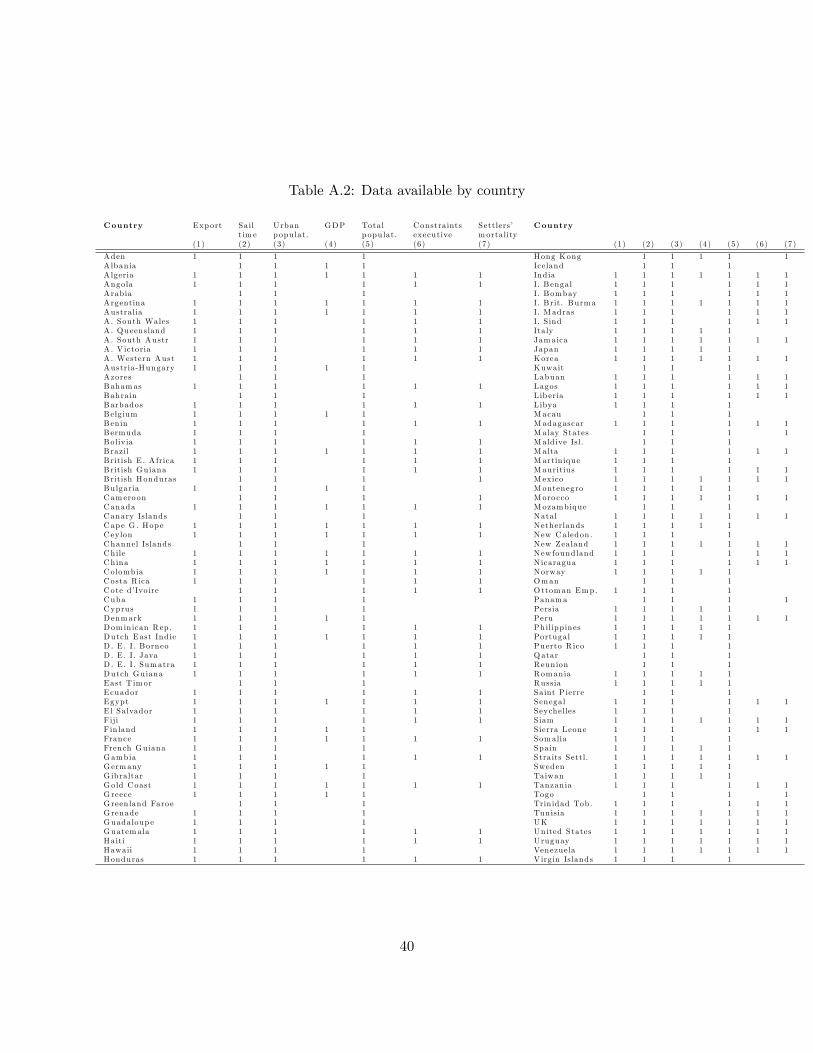
Table A.2: Data available by country

Country Export Sail U rban GDP Total Constra ints Settlers’ Countrytim e populat. p opulat. executive morta lity

(1) (2) (3) (4) (5) (6) (7) (1) (2) (3) (4) (5) (6) (7)

Aden 1 1 1 1 Hong Kong 1 1 1 1 1A lbania 1 1 1 1 Iceland 1 1 1A lgeria 1 1 1 1 1 1 1 India 1 1 1 1 1 1 1Angola 1 1 1 1 1 1 I. Bengal 1 1 1 1 1 1Arabia 1 1 1 I. Bombay 1 1 1 1 1 1Argentina 1 1 1 1 1 1 1 I. B rit. Burma 1 1 1 1 1 1 1Austra lia 1 1 1 1 1 1 1 I. M adras 1 1 1 1 1 1A . South Wales 1 1 1 1 1 1 I. S ind 1 1 1 1 1 1A . Queensland 1 1 1 1 1 1 Ita ly 1 1 1 1 1A . South Austr 1 1 1 1 1 1 Jamaica 1 1 1 1 1 1 1A . V ictoria 1 1 1 1 1 1 Japan 1 1 1 1 1A . Western Aust 1 1 1 1 1 1 Korea 1 1 1 1 1 1 1Austria-Hungary 1 1 1 1 1 Kuwait 1 1 1Azores 1 1 1 Labuan 1 1 1 1 1 1Bahamas 1 1 1 1 1 1 Lagos 1 1 1 1 1 1Bahrain 1 1 1 L ib eria 1 1 1 1 1 1Barbados 1 1 1 1 1 1 L ibya 1 1 1 1Belg ium 1 1 1 1 1 Macau 1 1 1Benin 1 1 1 1 1 1 Madagascar 1 1 1 1 1 1Bermuda 1 1 1 1 Malay States 1 1 1 1Boliv ia 1 1 1 1 1 1 Mald ive Isl. 1 1 1Brazil 1 1 1 1 1 1 1 Malta 1 1 1 1 1 1British E . A frica 1 1 1 1 1 1 Martin ique 1 1 1 1British Guiana 1 1 1 1 1 1 Mauritius 1 1 1 1 1 1British Honduras 1 1 1 1 M exico 1 1 1 1 1 1 1Bulgaria 1 1 1 1 1 Montenegro 1 1 1 1 1Cameroon 1 1 1 1 Moro cco 1 1 1 1 1 1 1Canada 1 1 1 1 1 1 1 Mozambique 1 1 1Canary Islands 1 1 1 Natal 1 1 1 1 1 1 1Cap e G . Hop e 1 1 1 1 1 1 1 Netherlands 1 1 1 1 1Ceylon 1 1 1 1 1 1 1 New Caledon . 1 1 1 1Channel Islands 1 1 1 New Zealand 1 1 1 1 1 1 1Chile 1 1 1 1 1 1 1 New foundland 1 1 1 1 1 1China 1 1 1 1 1 1 1 N icaragua 1 1 1 1 1 1Colombia 1 1 1 1 1 1 1 Norway 1 1 1 1 1Costa R ica 1 1 1 1 1 1 Oman 1 1 1Cote d’Ivoire 1 1 1 1 1 O ttoman Emp. 1 1 1 1Cuba 1 1 1 1 Panama 1 1 1 1Cyprus 1 1 1 1 Persia 1 1 1 1 1Denmark 1 1 1 1 1 Peru 1 1 1 1 1 1 1Dom in ican Rep. 1 1 1 1 1 1 Philipp ines 1 1 1 1 1Dutch East Ind ie 1 1 1 1 1 1 1 Portugal 1 1 1 1 1D . E . I. Borneo 1 1 1 1 1 1 Puerto R ico 1 1 1 1D . E . I. Java 1 1 1 1 1 1 Qatar 1 1 1D . E . I. Sumatra 1 1 1 1 1 1 Reunion 1 1 1Dutch Guiana 1 1 1 1 1 1 Romania 1 1 1 1 1East T imor 1 1 1 Russia 1 1 1 1 1Ecuador 1 1 1 1 1 1 Saint P ierre 1 1 1Egypt 1 1 1 1 1 1 1 Senegal 1 1 1 1 1 1E l Salvador 1 1 1 1 1 1 Seychelles 1 1 1 1F iji 1 1 1 1 1 1 S iam 1 1 1 1 1 1 1F in land 1 1 1 1 1 Sierra Leone 1 1 1 1 1 1France 1 1 1 1 1 1 1 Somalia 1 1 1 1French Guiana 1 1 1 1 Spain 1 1 1 1 1Gambia 1 1 1 1 1 1 Straits Settl. 1 1 1 1 1 1 1Germany 1 1 1 1 1 Sweden 1 1 1 1 1G ibraltar 1 1 1 1 Taiwan 1 1 1 1 1Gold Coast 1 1 1 1 1 1 1 Tanzania 1 1 1 1 1 1G reece 1 1 1 1 1 Togo 1 1 1 1G reen land Faro e 1 1 1 Trin idad Tob. 1 1 1 1 1 1G renade 1 1 1 1 Tunisia 1 1 1 1 1 1 1Guadaloup e 1 1 1 1 UK 1 1 1 1 1 1 1Guatemala 1 1 1 1 1 1 United States 1 1 1 1 1 1 1Haiti 1 1 1 1 1 1 Uruguay 1 1 1 1 1 1 1Hawaii 1 1 1 1 Venezuela 1 1 1 1 1 1 1Honduras 1 1 1 1 1 1 V irg in Islands 1 1 1 1

40

Table A.3: The shift from sail to steam 1

(1) (2) (3) (4)ln (exp ort) ln (exp ort) ln (exp ort) ln (exp ort)

ln(Steam D ist) x I(1855-1860) 0.265 0.0981 1.239(0 .465) (0 .492) (0 .920)(0 .480) (0 .480) (0 .847)(0 .197) (0 .202) (0 .468)***

ln(Steam D ist) x I(1860-1870) -0 .392 -0 .556 -0 .195 -0 .510(0 .267) (0 .325)* (0.157) (0 .422)(0 .310) (0 .325)* (0.122) (0 .462)(0 .111)*** (0.119)*** (0.0838)** (0.200)**

ln(Steam D ist) x I(1870-1880) -0 .759 -0 .922 -0 .370 -0 .872(0 .220)*** (0.288)*** (0.154)** (0.310)***(0.217)*** (0.270)*** (0.144)** (0.340)**(0 .0684)*** (0.0806)*** (0.0576)*** (0.0993)***

ln(Steam D ist) x I(1880-1890) -0 .868 -1 .034 -0 .410 -0 .862(0 .239)*** (0.301)*** (0.161)** (0.310)***(0.250)*** (0.316)*** (0.160)** (0.331)***(0.0640)*** (0.0773)*** (0.0549)*** (0.0887)***

ln(Steam D ist) x I(1890-1900) -0 .680 -0 .843 -0 .275 -0 .657(0 .238)*** (0.320)*** (0.179) (0 .275)**(0 .251)*** (0.329)** (0.193) (0 .303)**(0 .0611)*** (0.0745)*** (0.0533)*** (0.0815)***

ln(Sail D ist) x I(1855-1860) -0 .790 -0 .748 -1 .632(0 .482)* (0.477) (0 .987)*(0 .476)* (0.469) (0 .879)*(0 .202)*** (0.202)*** (0.446)***

ln(Sail D ist) x I(1860-1870) -0 .209 -0 .170 0.217 -0 .142(0 .278) (0 .274) (0 .163) (0 .445)(0 .296) (0 .291) (0 .128)* (0.481)(0 .114)* (0.115) (0 .0815)*** (0.201)

ln(Sail D ist) x I(1870-1880) 0.0148 0.0451 0.320 0.102(0.215) (0 .211) (0 .149)** (0.300)(0 .208) (0 .204) (0 .137)** (0.331)(0 .0682) (0 .0686) (0 .0495)*** (0.0976)

ln(Sail D ist) x I(1880-1890) 0.172 0.206 0.433 0.186(0.229) (0 .224) (0 .154)*** (0.293)(0 .243) (0 .242) (0 .143)*** (0.323)(0 .0633)*** (0.0640)*** (0.0460)*** (0.0873)**

ln(Sail D ist) x I(1890-1900) 0.0228 0.0547 0.383 -0 .0194(0.230) (0 .232) (0 .165)** (0.269)(0 .090) (0 .222) (0 .163)** (0.298)(0 .0602) (0 .0608) (0 .0441)*** (0.0797)

ln (Geo D ist) 0 .141(0.193)(0 .169)(0 .0368)***

COUNTRY FE YES YES NO NOYEAR FE YES YES YES NOPAIR FE NO NO YES NOCOUNTRY X YEAR FE NO NO NO YESR Squared 0.616 0.617 0.796 0.686Observations 23016 23016 23016 23016

The table reports OLS estimates on yearly data (1855-1900). The following standard errors are reported in paren-theses: 1) clustered at the country pair 2) clustered at the country of origin 3) robust; *** significant at less than 1percent; ** significant at 5 percent; * significant at 10 percent.

41

Table A.4: The shift from sail to steam 2

(1) (2) (3) (4)ln (exp ort) ln (exp ort) ln (exp ort) ln (exp ort)

ln(Steam D ist) x I(1855-1860) 0.278 0.110 1.239(0.470) (0 .496) (0 .921)(0 .486) (0 .485) (0 .848)(0 .197) (0 .202) (0 .468)***

ln(Steam D ist) x I(1860-1865) 0.0235 -0 .144 -0 .0271 0.400(0.403) (0 .432) (0 .199) (0 .808)(0 .488) (0 .474) (0 .203) (0 .837)(0 .213) (0 .217) (0 .157) (0 .484)

ln(Steam D ist) x I(1865-1870) -0 .530 -0 .695 -0 .252 -0 .673(0.249)** (0.315)** (0 .172) (0 .391)*(0.268)* (0.301)** (0.127)* (0.436)(0 .126)*** (0.133)*** (0.0949)*** (0.221)***

ln(Steam D ist) x I(1870-1875) -0 .719 -0 .884 -0 .341 -0 .867(0.222)*** (0.292)*** (0.156)** (0.317)***(0.212)*** (0.266)*** (0.142)** (0.359)**(0.0943)*** (0.103)*** (0.0746)*** (0.147)***

ln(Steam D ist) x I(1875-1880) -0 .794 -0 .958 -0 .399 -0 .876(0.225)*** (0.289)*** (0.162)** (0.314)***(0.235)*** (0.285)*** (0.166)** (0.333)***(0.0890)*** (0.0986)*** (0.0713)*** (0.135)***

ln(Steam D ist) x I(1880-1885) -0 .878 -1 .045 -0 .419 -0 .920(0.238)*** (0.296)*** (0.167)** (0.322)***(0.250)*** (0.312)*** (0.166)** (0.336)***(0.0867)*** (0.0968)*** (0.0698)*** (0.130)***

ln(Steam D ist) x I(1885-1890) -0 .856 -1 .024 -0 .405 -0 .812(0.248)*** (0.311)*** (0.168)** (0.319)**(0.260)*** (0.327)*** (0.166)** (0.345)**(0.0832)*** (0.0939)*** (0.0674)*** (0.121)***

ln(Steam D ist) x I(1890-1895) -0 .735 -0 .899 -0 .315 -0 .682(0.237)*** (0.319)*** (0.181)* (0.278)**(0.257)*** (0.336)*** (0.176)* (0.291)**(0.0799)*** (0.0904)*** (0.0653)*** (0.115)***

ln(Steam D ist) x I(1895-1900) -0 .624 -0 .788 -0 .236 -0 .634(0.245)** (0.327)** (0 .187) (0 .285)**(0.256)** (0.330)** (0 .223) (0 .334)*(0.0798)*** (0.0904)*** (0.0654)*** (0.115)***

ln(Sail D ist) x I(1855-1860) -0 .802 -0 .759 -1 .632(0.487)* (0.482) (0 .987)*(0.482)* (0.475) (0 .880)*(0.202)*** (0.202)*** (0.446)***

ln(Sail D ist) x I(1860-1865) -0 .534 -0 .492 0.0490 -0 .856(0.419) (0 .413) (0 .214) (0 .868)(0 .490) (0 .481) (0 .224) (0 .835)(0 .218)** (0.219)** (0 .159) (0 .468)*

ln(Sail D ist) x I(1865-1870) -0 .119 -0 .0813 0.272 -0 .0110(0.256) (0 .253) (0 .174) (0 .402)(0 .253) (0 .251) (0 .126)** (0.453)(0 .130) (0 .130) (0 .0934)*** (0.223)

ln(Sail D ist) x I(1870-1875) -0 .0232 0.00793 0.295 0.110(0.219) (0 .216) (0 .150)* (0 .308)(0 .204) (0 .201) (0 .141)** (0.352)(0 .0944) (0 .0947) (0 .0687)*** (0.144)

ln(Sail D ist) x I(1875-1880) 0.0465 0.0766 0.343 0.0941(0.218) (0 .213) (0 .158)** (0.304)(0 .226) (0 .220) (0 .153)** (0.325)(0 .0888) (0 .0892) (0 .0649)*** (0.133)

ln(Sail D ist) x I(1880-1885) 0.185 0.218 0.430 0.221(0.231) (0 .225) (0 .161)*** (0.308)(0 .243) (0 .241) (0 .152)*** (0.330)(0 .0861)** (0.0865)** (0.0630)*** (0.128)*

ln(Sail D ist) x I(1885-1890) 0.158 0.193 0.436 0.155(0.237) (0 .234) (0 .159)*** (0.302)(0 .254) (0 .255) (0 .147)*** (0.337)(0 .0825)* (0.0830)** (0.0601)*** (0.119)

ln(Sail D ist) x I(1890-1895) 0.0747 0.107 0.407 0.0304(0.228) (0 .230) (0 .165)** (0.270)(0 .251) (0 .254) (0 .150)*** (0.283)(0 .0790) (0 .0794) (0 .0577)*** (0.113)

ln(Sail D ist) x I(1895-1900) -0 .0305 0.00189 0.359 -0 .0666(0.238) (0 .240) (0 .173)** (0.283)(0 .251) (0 .253) (0 .190)* (0 .333)(0 .0787) (0 .0791) (0 .0578)*** (0.112)

ln (Geo D ist) 0 .142(0.193)(0 .170)(0 .0368)***

COUNTRY FE YES YES NO NOYEAR FE YES YES YES NOPAIR FE NO NO YES NOCOUNTRY X YEAR FE NO NO NO YESR Squared 0.617 0.617 0.796 0.687Observations 23016 23016 23016 23016

The table reports OLS estimates on yearly data (1855-1900). The following standard errors are reported in paren-theses: 1) clustered at the country pair 2) clustered at the country of origin 3) robust; *** significant at less than 1percent; ** significant at 5 percent; * significant at 10 percent.

42

Table A.5: Trade and Urbanization Rates - Reduced form

(1) (2) (3) (4) (5) (6)Urban Pop (>25000) Urban Pop (>50000) Urban Pop (>100000))

Log Pred. -0.0240*** -0.0247*** -0.0369*** -0.0384*** -0.0325*** -0.0343***Trade (0.0105) (0.00971) (0.00980) (0.0100) (0.0109) (0.0110)COUNTRY DUMMIES YES YES YES YES YES YESYEAR DUMMIES YES YES YES YES YES YESr2 0.941 0.935 0.954 0.942 0.948 0.933N 702 702 702 702 702 702WEIGHTED NO YES NO YES NO YES

The table reports OLS estimates. The unit of observation is country-year. The dependent variable is the log ofthe population share living in cities with more than either 25,000 citizens (columns 1 and 2), or 50,000 citizens(columns 3 and 4), or 100,000 citizens (columns 5 and 6). "Log Predict Trade" is constructed according to equation6. Observations are un-weighted in columns 1,3 and 5 and weighted by the log-population of the country in columns2, 4 and 6. Standard errors (reported in parentheses) are two-way clustered (country and year). *** significant atless than 1 percent; ** significant at 5 percent; * significant at 10 percent.

Table A.6: Trade and Urbanization: the Role of Local Institutions - Instrumenting Institutions

(1) (2) (3) (4) (5) (6) (7) (8)Urb. Pop (>25t) Urb. Pop (>50t) Urb. Pop (>100t) Population

Log Trade -0.200* -0.183* -0.182* -0.183 -0.189 -0.173* -3.320*** -2.819***(0.103) (0.0937) (0.109) (0.112) (0.119) (0.0985) (0.940) (0.750)

Log Trade 0.333*** 0.356*** 0.301*** 0.381*** 0.338*** 0.330*** 3.636*** 3.184**** Good Inst (Polity>=3) (0.124) (0.121) (0.139) (0.171) (0.167) (0.133) (0.918) (0.822)COUNTRY DUMMIES YES YES YES YES YES YES YES YESYEAR DUMMIES YES YES YES YES YES YES YES YESF 3.327 3.040 3.327 3.040 3.327 3.040 3.392 2.917N 312 312 312 312 312 312 320 320r2 0.718 0.670 0.755 0.525 0.647 0.683 0.941 0.954WEIGHTED NO YES NO YES NO YES NO YES

The table reports 2SLS. The unit of observation is country-year. The dependent variable is the log of the populationshare living in cities with more than either 25,000 citizens (columns 1 and 2), or 50,000 citizens (columns 3 and4), or 100,000 citizens (columns 5 and 6) or the log of population density (columns 7 and 8). "Log Trade" is thelog of per-capita trade (import plus export)."Good Inst" is a dummy that is equal to 1 if the POLITY IV variable?Constraints on the executive? was not lower than 3 in 1860. The excluded instrument is constructed according toequation 6. Observations are un-weighted in columns 1,3, 5 and 7 and weighted by the log-population of the countryin columns 2, 4, 6 and 8. F is the F statistics for weak identification. Standard errors (reported in parentheses) aretwo-way clustered (country and year). *** significant at less than 1 percent; ** significant at 5 percent; * significantat 10 percent.

43

Figure A.1: The Change in Elasticity of Trade with Respect to Shipping Times by Sail and SteamVessels (Estimates from a gravity model with country and year fixed effects)

Figure A.2: The Change in Elasticity of Trade with Respect to Shipping Times by Sail and SteamVessels (Estimates from a gravity model with country by year fixed effects)

44

Figure A.3: The Change in Elasticity of Trade with Respect to Shipping Times by Sail and SteamVessels (Estimates from a gravity model with country pair and year fixed effects)

45