Working Papers|070| August 2006

Jože P. Damijan, José de Sousa and Olivier Lamotte

The Effect of Trade Liberalization in South-Eastern European Countries

The wiiw Balkan Observatory

www.balkan-observatory.net

About Shortly after the end of the Kosovo war, the last of the Yugoslav dissolution wars, theBalkan Reconstruction Observatory was set up jointly by the Hellenic Observatory, theCentre for the Study of Global Governance, both institutes at the London School ofEconomics (LSE), and the Vienna Institute for International Economic Studies (wiiw).A brainstorming meeting on Reconstruction and Regional Co-operation in the Balkanswas held in Vouliagmeni on 8-10 July 1999, covering the issues of security,democratisation, economic reconstruction and the role of civil society. It was attendedby academics and policy makers from all the countries in the region, from a number ofEU countries, from the European Commission, the USA and Russia. Based on ideas anddiscussions generated at this meeting, a policy paper on Balkan Reconstruction andEuropean Integration was the product of a collaborative effort by the two LSE institutesand the wiiw. The paper was presented at a follow-up meeting on Reconstruction andIntegration in Southeast Europe in Vienna on 12-13 November 1999, which focused onthe economic aspects of the process of reconstruction in the Balkans. It is this policypaper that became the very first Working Paper of the wiiw Balkan ObservatoryWorking Papers series. The Working Papers are published online at www.balkan-observatory.net, the internet portal of the wiiw Balkan Observatory. It is a portal forresearch and communication in relation to economic developments in Southeast Europemaintained by the wiiw since 1999. Since 2000 it also serves as a forum for the GlobalDevelopment Network Southeast Europe (GDN-SEE) project, which is based on aninitiative by The World Bank with financial support from the Austrian Ministry ofFinance and the Oesterreichische Nationalbank. The purpose of the GDN-SEE projectis the creation of research networks throughout Southeast Europe in order to enhancethe economic research capacity in Southeast Europe, to build new research capacities bymobilising young researchers, to promote knowledge transfer into the region, tofacilitate networking between researchers within the region, and to assist in securingknowledge transfer from researchers to policy makers. The wiiw Balkan ObservatoryWorking Papers series is one way to achieve these objectives.

The wiiw Balkan Observatory

Global Development Network Southeast Europe

This study has been developed in the framework of research networks initiated and monitored by wiiwunder the premises of the GDN–SEE partnership. The Global Development Network, initiated by The World Bank, is a global network ofresearch and policy institutes working together to address the problems of national andregional development. It promotes the generation of local knowledge in developing andtransition countries and aims at building research capacities in the different regions. The Vienna Institute for International Economic Studies is a GDN Partner Institute andacts as a hub for Southeast Europe. The GDN–wiiw partnership aims to support theenhancement of economic research capacity in Southeast Europe, to promoteknowledge transfer to SEE, to facilitate networking among researchers within SEE andto assist in securing knowledge transfer from researchers to policy makers. The GDN–SEE programme is financed by the Global Development Network, theAustrian Ministry of Finance and the Jubiläumsfonds der OesterreichischenNationalbank. For additional information see www.balkan-observatory.net, www.wiiw.ac.at andwww.gdnet.org

The wiiw Balkan Observatory

The effect of trade liberalization in South-EasternEuropean countries∗

Joze Damijan† Jose de Sousa‡ Olivier Lamotte§

August 1st, 2006

Abstract

South-Eastern European (SEE) countries have recently engaged in a re-gional integration process, through the establishment of free trade agree-ments between themselves and with the European Union (EU). This studyevaluates the impact of this process on trade and firm performance.

Three complementary approaches are used. The first consists in eval-uating the degree of trade integration of SEE countries and determiningtheir trade potential with their main partners, i.e. themselves and the EU.The second approach tries to evaluate the evolution of tariffs and nontariffsbarriers, faced by SEE countries and estimate their effects on manufacturedtrade. The third part investigates the impact of trade liberalization on per-formance of firms in SEE. In particular, we are interested in what extentforeign trade and foreign direct investment contributed to improvements infirm performance.

Several interesting results emerge from this study. Concerning our firstapproach, we find three results. First, Western Balkan countries have reachedtheir trade potential for almost all sectors while Eastern Balkan countrieshave outreached them. One can therefore expect an increase of trade flowsbetween the Western Balkans and the EU. Second, it seems that preferentialtrade agreements between SEE countries will have a limited impact on theirmutual trade since their trade potentials are already reached. Third, allSEE countries’ trade is below its potential with the rest of the world.

∗This report has been completed within the framework of the Global Development Networkproject supervised by the WIIW (Austria). We thank Mario Holzner, Robert Stehrer and par-ticipants at two WIIW workshops for helpful comments and discussions.

†University of Ljubljana and Licos, University of Leuven, E-mail: joze.damijan@ef.uni-lj.si‡CES-EureQua, University of Paris 1, E-mail: jdesousa@univ-paris1.fr§CES-EureQua, University of Paris 1.

1

Concerning our second approach, we find that exports are increasing inall sectors during the period 1996-2000, while bilateral tariffs are decreasing.However, this liberalization process exhibits small effects on trade. On theother hand, we find that nontariff barriers are increasing during the period.Trade liberalization should not be treated as exogenous (Trefler, 1993). Do-mestic firms, competiting with Balkan exporters, may have increased theirlobbying activity for greater protection. As a result, NTBs increase andhurt exports of Balkan countries. In that respect, we find large estimates ofNTBs on exports of manufactured goods.

Concerning our third approach, we do not find a general pattern of uni-formly significant impact of extensive trade flows on individual firm’s TFPgrowth. Specifically, only in Romania and Slovenia, higher propensity toexport to advanced markets (EU-15, rest of OECD countries) has a largerimpact on TFP growth than exporting to less advanced markets such asnew EU members and countries of former Yugoslavia. The role of importsfollows a similar path as exporting. Importing from the advanced countriesis important for firms in Romania. At the same time, for firms in Romaniaand Macedonia importing from countries of former Yugoslavia provides adominating learning effect. For other countries in our sample no learningeffects from exporting to and importing from individual geographic regionscould be found. Thus, one cannot imply that liberalization of bilateral tradewithin the region of SEE or with the other regions will have uniformly signif-icant impact on individual firm’s performance, but in some of the countriesanalysed trade liberalization might be an important engine of firms’ produc-tivity growth.

Our results also indicate some selection process in FDI decisions by par-ent foreign companies. Foreign parent companies seem to select smaller firmsin SEE as well as least productive, less capital and skill intensive firms. How-ever, we find contrasting results on the impact on foreign ownership on TFPgrowth. Three countries (Bosnia, Croatia and Slovenia) experience fasterTFP growth in foreign owned firms. In Romania, in contrast we find fasterTFP growth in domestic owned firms, while in Bulgaria no significant dif-ferences have been found. However, one can expect that after restructuringthese firms would improve their TFP at a much faster rate than purely do-mestic owned firms.

Key-words: trade potential, trade liberalization, gravity equation, pref-erential trade agreements, South-Eastern Europe.

JEL Classification: C13, C23, F15, F17

2

Contents

1 Introduction 5

2 Regional integration 82.1 Measures of trade liberalization between the EU and SEE countries 92.2 Trade integration between SEE countries . . . . . . . . . . . . . . . 11

3 An estimation of trade potentials of South-Eastern European coun-tries 143.1 Trade potentials in the literature . . . . . . . . . . . . . . . . . . . 143.2 Empirical model and data . . . . . . . . . . . . . . . . . . . . . . . 173.3 Estimations on aggregated data . . . . . . . . . . . . . . . . . . . . 193.4 Estimations on disaggregated data . . . . . . . . . . . . . . . . . . 26

4 The impact of trade liberalization on trade flows 334.1 Basic statistics . . . . . . . . . . . . . . . . . . . . . . . . . . . . . 344.2 Empirical model . . . . . . . . . . . . . . . . . . . . . . . . . . . . . 374.3 Results . . . . . . . . . . . . . . . . . . . . . . . . . . . . . . . . . . 384.4 Robustness checks . . . . . . . . . . . . . . . . . . . . . . . . . . . . 424.5 Summary estimates . . . . . . . . . . . . . . . . . . . . . . . . . . . 43

5 The impact of trade liberalization on firm performance 445.1 Descriptive statistics . . . . . . . . . . . . . . . . . . . . . . . . . . 455.2 Empirical model and methodology . . . . . . . . . . . . . . . . . . . 50

5.2.1 Modelling impact of FDI and trade effects on firm performance 505.3 Econometric issues . . . . . . . . . . . . . . . . . . . . . . . . . . . 515.4 Results . . . . . . . . . . . . . . . . . . . . . . . . . . . . . . . . . . 55

5.4.1 Results with first differences estimation . . . . . . . . . . . . 555.4.2 Results with system GMM estimation . . . . . . . . . . . . . 58

6 Concluding remarks 61

7 Appendix 73

List of Tables

1 Classification of the free trade agreements according to the degreeof trade liberalization . . . . . . . . . . . . . . . . . . . . . . . . . . 13

2 Recent literature using trade potentials . . . . . . . . . . . . . . . . 153 Estimates on aggregated data, estimations (1)-(4). . . . . . . . . . . 20

3

4 Ratio actual trade/potential trade on aggregated data, in %. . . . . 225 Results on aggregated data, estimations (5)-(6). . . . . . . . . . . . 246 Estimates by sector, estimations (7)-(16). . . . . . . . . . . . . . . . 277 Estimates by sector, estimations (17)-(26). . . . . . . . . . . . . . . 318 Actual/potential trade ratio by sector, in %. . . . . . . . . . . . . . 329 Tariff barriers estimates . . . . . . . . . . . . . . . . . . . . . . . . 3910 Tariff barriers estimates including production by sectors . . . . . . . 4011 Nontariff and tariff barriers estimates . . . . . . . . . . . . . . . . . 4012 Nontariff barriers estimates . . . . . . . . . . . . . . . . . . . . . . 4113 Tariff barriers estimates - Robustness checks . . . . . . . . . . . . . 4214 Nontariff barriers estimates - Robustness checks . . . . . . . . . . . 4315 Range of estimates of TBs and NTBs on trade (in percent). . . . . 4416 Number of domestic and foreign owned firms and relative wages and

value added, 1994 - 2002. . . . . . . . . . . . . . . . . . . . . . . . . 4617 Regional export shares, 1994 - 2002, in %. . . . . . . . . . . . . . . 4818 Regional import shares, 1994 - 2002, in %. . . . . . . . . . . . . . . 4919 Heckman probit estimates . . . . . . . . . . . . . . . . . . . . . . . 5420 Average rates of growth of value added, labor and value added per

employee in SEE, 1994-2002, in %. . . . . . . . . . . . . . . . . . . 5621 Impact of FDI and export propensity on productivity growth in

SEE firms, period 1995 - 2002 (first differences specification). . . . . 5722 Impact of FDI, export and import propensity on productivity growth

in SEE firms, period 1995 - 2002. . . . . . . . . . . . . . . . . . . . 5923 Impact of FDI, export and import propensity on productivity growth

in SEE firms, period 1995 - 2002, system GMM estimations. . . . . 6024 Free trade agreements between SEE countries . . . . . . . . . . . . 7325 Review of the literature using sectoral estimations of the gravity

equation . . . . . . . . . . . . . . . . . . . . . . . . . . . . . . . . . 7426 SEE countries and the WTO . . . . . . . . . . . . . . . . . . . . . . 7527 Initiatives of regional cooperation in South-Eastern Europe . . . . . 7628 List of the countries of the sample . . . . . . . . . . . . . . . . . . . 7829 CHELEM-CEPII sectoral classification of international trade, 10

sectors. . . . . . . . . . . . . . . . . . . . . . . . . . . . . . . . . . . 7930 CHELEM-CEPII sectoral classification of international trade, 69

products. . . . . . . . . . . . . . . . . . . . . . . . . . . . . . . . . 80

4

1 Introduction

The dissolution of the Council of Mutual Economic Assistance (CMEA) and of the

Socialist Federative Republic of Yugoslavia (SFRY) in 1991 have deeply affected

economic and trade flows of South-Eastern Europe1 (SEE) countries. They also

have created incentives for a reshaping of trade patterns in the region. The topic

of regional trade integration in SEE countries has been largely debated at the

end of the 1990s. Some authors have advocated the creation of a free trade area

between Successor States of former Yugoslavia. They argued that their poor export

performances towards the EU could be compensated by an increase of their mutual

exports (Kovac, 1998; Uvalic, 2001). Other authors have considered that this

trade policy would have limited economic gains and was risky for the most fragile

economies of the region (Kaminsky and de la Rocha, 2003).

New initiatives aimed at creating a dynamic of trade reintegration to the world

economy have been launched during the mid 1990s. The dynamic of trade liber-

alization first took the form of a progressive reintegration of South-Eastern Euro-

pean countries to the World Trade Organization (WTO). Until the 1st of October,

2005 all SEE countries are WTO members except Bosnia-Herzegovina and Serbia-

Montenegro2. But, more importantly, this dynamic took place at regional and

sub-regional levels. For Bulgaria and Romania, regional economic integration with

the EU took the form of cooperation agreements between 1990 and 1993 and then

association agreements aimed at creating a free trade area. For other SEE coun-

tries, Stabilization and Association agreements have entered in force since 2001.

At the same time a sub-regional process of economic integration has emerged. On

one hand, Bulgaria and Romania have liberalized their trade in the framework of

the Central European Free Trade Agreement (CEFTA) signed in 1997. On the

other hand, a set of bilateral trade agreements have entered in force between all

SEE countries at the beginning of the 2000s.

This study evaluates the impact of the integration process of SEE countries.

Three complementary approaches are used. The first consists in evaluating the

degree of their trade integration between 1994 and 2002, and determining their

1South-Eastern Europe refers to Western Balkans (Albania, Bosnia-Herzegovina, Croatia,Macedonia, Serbia-Montenegro) and Eastern Balkans (Bulgaria and Romania).

2Situations of each country towards the WTO are presented in Table (26) in appendix.

5

trade potential with their main partners, i.e. themselves and the EU. We can

therefore identify potential gains of trade linked to the regional integration process.

The second approach first tries to evaluate the evolution of tariffs and nontariffs

barriers, faced by SEE countries, between 1996 and 2000, and to estimate their

effects on manufactured trade. The third part investigates the impact of trade

liberalization on performance of firms. In particular, we are interested in what

extent foreign trade and foreign direct investment contributed to improvements in

firm performance over the period 1995-20023.

In our first approach, the calculation of trade potentials is based on the esti-

mation of a gravity equation. This method has been largely used to determine

ex ante and ex post the effects of preferential trade agreements or, in the case of

Eastern European countries, the effects of international openness. The calculation

of trade potentials allows comparing the intensity of trade flows of a country pair

or a country group to a sample which constitutes the counterfactual. The choice

of the reference sample represents a crucial step (Fontagne and alii, 2002) and

depends of the goal of the study. Two dimensions must be taken into account: the

sample of countries and the time period.

Many recent articles have studied trade reorientation of Central European coun-

tries during the 1990s but very few authors have studied trade flows of SEE coun-

tries. Some exceptions are noticeable. Christie (2002) evaluates the trade potential

of SEE countries by estimating a gravity equation and simulating the evolution of

their national income. The author identifies an unbalanced integration in 1996-

1999, since trade flows are much higher or much lower than their “natural” level.

Kaminski and de la Rocha (2003) show, through a gravity equation, that there is

no potential for the increase of trade flows between SEE countries but a poten-

tial with other European countries. These two studies use cross-section data and

techniques, which do not take account for the time dimension or the country het-

erogeneity. This elements are particularly important as the countries of the region

have known episodes of conflicts and sanctions in the 1990s, which have deeply

affected their trade flows.

Our approach concerning the computation of trade potential is different and

3The three different approaches retain three different periods due to severe data constraintson the 1994-2002 period (see below).

6

our contribution stands at three levels. First we highlight the effects of the recent

process of trade liberalization between SEE countries and between themselves and

the EU. Second, we use panel data and panel techniques. We use the Hausman-

Taylor (1981) methodology, which allows taking account the endogeneity of free

trade agreements4. Thirdly, our estimations are based on sectoral data, which al-

lows taking account trade specialization and to evaluate trade liberalization limited

to some sectors.

With respect to our second approach, concerning the effects of tariffs and non-

tariffs barriers on manufactured trade flows, we get also interesting results. We

find that exports are increasing in all sectors during the period 1996-2000, while

bilateral tariffs are decreasing. However, this liberalization process exhibits small

effects on trade. In other hand we find that, if tariffs are decreasing, nontariff bar-

riers are increasing during the period. Trade liberalization should not be treated as

a given (Trefler, 1993). Domestic firms, competiting with Balkan exporters, may

have increased their lobbying activity for greater protection. As a result, NTBs

increase and hurt exports from Balkan countries. In that respect, we find large

estimates of NTBs on exports of manufactured goods.

Concerning our third approach, we investigate different sources of potential

outward knowledge spillovers that may be important determinant of productivity

growth of individual firms. International trade is an obvious channel of technology

transfer, in particular imports of intermediate products and capital equipment (see

Markusen, 1989; Grossman and Helpman, 1991; Feenstra, Markusen and Zeile,

1992) as well as through learning by exporting into industrial countries (Clerides,

Lach and Tybout, 1998). Firms exporting to more advanced markets can learn

more through exports due to higher quality, technical, safety and other standards

they have to meet as well as due to tougher competition (and lower markups).

Similarly, firms importing capital and intermediate inputs from more advanced

markets have to meet according technical standards to use the advanced western

technology. Hence, higher propensity to trade with more advanced countries should

obviously result in higher level of productivity and faster TFP growth.

We find that, in Romania and Slovenia, higher propensity to export to advanced

markets (EU-15, rest of OECD countries) has a larger impact on TFP growth

4See on this point Baier and Bergstrand (2003, 2004).

7

than exporting to less advanced markets such as new EU members and countries

of former Yugoslavia. In other words, exporting to advanced countries provide

much larger learning effects for a typical firm than exporting to less advanced

markets. The role of imports follows a similar path as exporting. Importing from

the advanced EU and OECD countries is important for firms in Romania. Thus,

in terms of policy implications, trade liberalization within the region of SEE might

be an important engine of firms’ growth in some of the countries.

Another obvious channel is the form of ownership, foreign vs. domestic. Dami-

jan et alii (2003) demonstrate that direct effect of foreign ownership is by far the

most dominating effect over horizontal or vertical spillovers from foreign ownership

in the economy. Firms that are foreign owned are better managed and governed,

have access to up-to-date technology of the parent firm and can use the business

links of the parent firm. Our results also indicate some selection process in FDI

decisions by parent foreign companies. Foreign parent companies seem to select

smaller firms in SEE as well as least productive, less capital and skill intensive

firms. However, we find contrasting results on the impact on foreign firms on

TFP growth. Three countries (Bosnia, Croatia and Slovenia) experience faster

TFP growth in foreign owned firms. In Romania, in contrast we find faster TFP

growth in domestic owned firms, while in Bulgaria no significant differences have

been found. However, one can expect that after restructuring these firms would

improve their TFP at a much faster rate than purely domestic owned firms.

In section 2, we present the regional trade process in South-Eastern Europe.

In section 3, we compute trade potentials. In section 4, we evaluate the effects of

tariffs and nontariffs barriers on trade. In section 5, we investigate the impact of

trade liberalization on firm performance. In the last section, we conclude.

2 Regional integration

Since the beginning of the 1990s, some initiatives aimed at creating a dynamic of

regional integration in South-Eastern Europe have emerged. For several reasons

presented in the core of this paper, these initiatives have not led to the creation of

an institutional framework that could enhance trade flows of the countries of the

region. This dynamic has however been renewed by the creation of the Stability

8

Pact for South-Eastern Europe in 1999, at the initiative of the EU. Actually, the

process of reconciliation and regional cooperation constitutes “the cornerstone of

the EU policy for the region” (Commission of the European Communities, 2003)

and it constitutes the core of the Pact for the stabilization, the reconstruction, and

the transformation of the Balkan economies5. Foreign trade promotion was devel-

oped through two main initiatives: the stabilization and association agreements

(sub-section 1), and the free trade agreements between the beneficiary countries of

the Stability Pact, initiated by the Memorandum of Understanding on Trade and

Transport Facilitation7 (sub-section 2).

2.1 Measures of trade liberalization between the EU and

SEE countries

The process of stabilization and association is a component of the Stability Pact

and includes trade measures as well as measures aimed at favoring the political,

economical, financial and humanitarian cooperation. Concerning trade measures,

the relationships of the beneficiary countries and the EU have been reinforced

by two kinds of measures: the asymmetric trade preferences from 2000 and the

stabilization and association agreements.

The first package of measures has been consigned in the regulation (EC) 2007 /

2000 of the EU which introduces free access to the EU for the products originating

from the SEE countries8. There are very few restrictive measures and they take the

5The Stability Pact for South-Eastern Europe was created at the aftermath of the Kosovo warand the NATO bombings to propose long run solutions for Western Balkans. This approach washighly necessary since SEE countries had not, to the contrary of Eastern European countries,intense and new relationships with the EU (Van Brabant, 2001). On 30 June 1999, the leaders of39 countries and the representatives of 17 international organizations met in Sarajevo to adoptthe Stability Pact for South-Eastern Europe, engaging themselves to sustain the stabilizationand the reconstruction of the region. Seven countries benefited from the financial assistance:Albania, Bosnia and Herzegovina, Bulgaria, Croatia, Romania, Macedonia and Federal Republicof Yugoslavia (FRY)6. Because of the high number of implied actors the Stability Pact constituteswhat Welfens qualifies the “ the most complex political initiative of the 20th century ” (Welfens,2001, p.9). The Pact is organized around three working tables: (1) democratization and humanrights, (2) economic reconstruction, development and cooperation and (3) intern and externsecurity.

7The full text of the Memorandum is available at the EU-WB common website for South-Eastern Europe: www.seerecon.org/ttfse/.

8“ Products originating in the Republics of Albania, Bosnia and Herzegovina and Croatia as

9

form of quantitative restrictions for the textile products originating from Serbia-

Montenegro, some fish products, some wines and sugar originating from these

countries.

In terms of trade liberalization, Stabilization and Association agreements con-

stitute the main device of the Stability Pact for South-Eastern Europe. They have

been signed by Croatia and Macedonia in 2001, other countries being at the stage

of negotiations9. The content of these agreements is very close to the content of

the Association Agreements signed in the 1990s between the EU and the Cen-

tral and Eastern European countries. They establish a free trade area within 6

years. Tariffs and quantitative restrictions are suppressed immediately except for a

small number of products for which the tariff reduction is progressive. It concerns

chemicals, textile, steel, agricultural and fishery products10.

A certain number of gains are expected from such a trade liberalization process.

They can lead to trade creation with the EU countries and to trade diversion

with other countries and in particular with SEE countries. This justifies the EU

pressure for the development of sub-regional free trade agreements. Since the

majority of free trade agreements are realized with the European countries11 trade

diversion to tier countries will be limited. We can also expect dynamic gains,

notably through market enlargement. However, the EU trade policy towards the

SEE countries are mainly motivated by non trade gains. A deeper integration to

the EU leads to import the EU institutions, accelerate the structural reforms and

make them irreversible. Moreover it constitutes a mean to liberalize trade flows of

these countries out of the multilateral framework.

This economic integration with the EU was linked, as from as the establishment

of the Stability Pact for South-Eastern Europe, to the development of the sub-

regional cooperation, notably in the field of trade liberalization. Integration to the

well as in Kosovo [...] shall be admitted for import into the Community without quantitativerestrictions or measures having equivalent effect and with exemption from customs duties andcharges having equivalent effect” (Regulation EC 2007/2000).

9On the advancement of negotiations with other countries see the Report of the Commissionof 30 March 2004; “The Stabilization and Association Process for South-Eastern Europe”, ThirdAnnual Report, COM(2004) 202 Final.

10Commission of the European Community, COM(2001), 371 Final.11In 2002, more than 80% of the trade of SEE countries are realized with European countries

(Lamotte, 2003).

10

EU has to be accompanied by a mutual integration process for two main reasons

(Kaminski and de la Rocha, 2003). First, a hub and spoke type regional integration

process, i.e. only oriented only towards the EU, could benefit only to EU firms,

to the detriment of SEE firms. EU firms has the advantage to have access to

all markets of South-Eastern Europe while the latter have not a free access to

SEE markets. Second, free trade agreements need the establishment of rules of

origins to avoid the development of transit trade. These rules provide another

supplementary advantages to EU firms: (i) they have access to a higher number of

intrants locally, to the contrary of SEE firms that depend from imports for their

production, (ii) they don’t support supplementary costs due to the justification

of the origins of their intrants since they are already embedded in a network of

preferential trade agreements, (iii) firms of South-Eastern Europe are specialized

in sensitive sectors (Astrov, 2001) for which the justification of the origin is more

complex, notably because the technical criteria for production are required for this

kind of products.

One of the remedies to the negative effects of regional integration between

the EU and the SEE lies in the set up of preferential trade agreements between

SEE countries themselves. However this should not constitute an alternative to

the deepening of integration to the EU, notably because the small size of SEE

economies does not allow foreseeing important benefits of trade integration between

these countries (World Bank, 2000).

2.2 Trade integration between SEE countries

Since the beginning of the 1990s, many authors advocated the development of re-

gional cooperation between SEE countries12. The disintegration of the economic

areas in Eastern Europe has deeply affected trade flows. The reinsertion of Balkan

economies in a network of institutional links aimed at enhancing trade became a

priority. Moreover, the idea according to which economic dependance is a factor

12The first known experience of regional trade integration between SEE countries dates fromthe end of the nineteenth century. The Balkan Conferences took place between 1930 and 1933.They led to the creation of a regional economic agreement aimed at reducing trade barriersbetween the Balkan States. An exhaustive presentation of regional integration process in SEE isprovided in Lopandic (2001).

11

of peace still prevails since the World War II, even if the strong dependency of

Yugoslav Republics did not prevent a violent disintegration. A plethora of multi-

lateral initiatives has emerged in the 1990s13 (Daianu and Veremis, 2001). None of

them gave convincing results in terms of economic cooperation (Lopandic, 1999).

This can be explained by three main reasons (Lamotte, 2003): the poor finan-

cial and human resources of the country members, the low support of the foreign

partners, the political tensions and the mutual distrust between countries, and

finally the absence of Serbia-Montenegro in these arrangements. The democratic

turn-point engaged by Serbia-Montenegro after the overthrow of Milosevic the 5

October 2000 has opened new perspectives.

The Memorandum of Understanding on Trade and Transport Facilitation signed

between the Ministries of Foreign Affairs of seven countries of South-Eastern Eu-

rope the 27 June 2001 in Brussels, advocated the set up of 21 free trade agreements

between these countries by the end 200214. It led to an important movement of

trade liberalization during the past four years, both on a bilateral and on a multi-

lateral basis15. Since the beginning of 2005, all trade flows in the region are realized

in the framework of free trade agreements. Practically, these agreements provided

(i) the elimination of tariffs on 90% of the volume of trade and 90% of the tariffs

lines, (ii) the elimination of non tariffs barriers to trade for intra-regional trade

and the strengthening of trade in services and (iii) the facilitation in trade (Bjelic,

2005).

Free trade agreements can be classified according to the degree of liberalization

they reached (Messerlin and Miroudot, 2004). The classification of agreements

according to the criteria (i) is presented in Table (1). One third of the agreements

satisfies the criteria of liberalization of 90% of the volume of trade and of 90% of

the tariff line, one third satisfies one the two criteria and the last third does not

satisfy any of the criteria. One should notice that there are differences in terms

of tariff concessions between manufactured and agricultural products. Trade of

industrial products is almost completely free. On the other hand, for agricultural

13They are presented in the Table ??? 12, in appendix.14The process of cooperation with Moldova started later but it also led to the creation of trade

agreements.15The dates of entry in force of the mutual trade agreements between SEE countries are

presented in Table (24) in appendix.

12

products, tariffs concessions granted in the framework of the second and third types

(cf. Table 1) cover only a small part of the traded goods. Finally, it is important

to note that trade liberalization for agricultural goods is often asymetric. The

most striking example concerns the free trade agreement between Bulgaria and

Serbia-Montenegro. The first has eliminated its tariffs on 45% of its imports from

Serbia-Montenegro, while only 2,5% of Bulgarian exports to Serbia-Montenegro

are tariffs-free (Messerlin and Miroudot, 2004).

Table 1: Classification of the free trade agreements according to the degree of tradeliberalization

Degree of liberalization Bilateral free trade agreementsGroup 1 Agreements fulfilling the cri-

teria of liberalization of 90%of the volume of trade and90% of the tariff lines

BIH-HRV, BIH-MKD, BIH-MDV, BIH-SCG,BGR-HRV, BGR-ROM, MKD-SCG, MLD-ROM

Group 2 Agreements fulfilling one ofthe 90% criteria

90% of the volume oftrade:

90% of the tariff lines:

ROM-SCG ALB-BIH, ALB-MKD,ALB-SCG, BIH-BGR,BIH-ROM, HRV-MKD, HRV-SCG

Group 3 Agreements fulfilling none ofthe 90% criteria

ALB-BGR, ALB-HRV, ALB-ROM, BGR-MKD, BGR-SCG, HRV-ROM, MKD-ROM

Notes: Table based on Messerlin and Miroudot (2004). Five free-trade agree-ments are not classified by the authors. Countries are signaled by their ISOcodes: BIH=Bosnia-Herzegovina, BGR=Bulgaria, HRV=Croatia, MKD=Macedonia,MLD=Moldova, ROM=Romania, SCG=Serbia-Montenegro.

However, such agreements raise some problems. First the bilateral approach

led to a complex structure of concessions and to different agenda. This could be

avoided if trade liberalization was realized in a multilateral framework (Adam et

alii, 2003). The complexity of the agreements is reinforced by the asymetry of the

trade preferences. Second, one can expect limited gains from trade in terms of

convergence because of the low income per capita of these countries. Moreover,

such a process increases the risk of a shift of the industry from the lower income

countries to the higher income countries (Kaminski and de la Rocha, 2003). A

concentration of the industry in the highest income country, Croatia, can be ex-

pected. However, this effect might be limited. Actually, after trade liberalization,

firm’s location becomes more and more sensible to labor cost differences (Puga

13

and Venables, 1998). It is therefore not sure that a shift in industry location to

the high-income country will take place. Moreover, Croatia is, along with Bulgaria

and Romania, likely to entry in the EU soon, and therefore to converge quickly

towards the EU in terms of income per capita.

We showed that SEE countries are embedded in a network of free trade agree-

ments which will determine the evolution of the structure of their trade. In the

next section, we present the techniques and the data used for the study of these

agreements.

3 An estimation of trade potentials of South-

Eastern European countries

3.1 Trade potentials in the literature

The calculation of trade potentials to evaluate the degree of regional economic

integration is one of the most frequent use of the gravity equation (Greenaway and

Milner, 2002). The theoretical foundations of the gravity equation has been re-

newed recently, both from monopolistic competition (Baier and Bergstrand, 2003,

2004) and perfect competition (Anderson and Van Wincoop, 2003) frameworks.

Empirical works using the calculation of trade potentials have known an important

development during the last 15 years, because of the proliferation of preferential

trade agreements and the openness of former socialist countries to the world econ-

omy. A high number of articles deals with the trade potential of Eastern and

Central European countries and the EU (Table 2).

The calculation of trade potentials from the gravity equation lies on two ap-

proaches: the in-sample and the out-of-sample approach. The out-of-sample ap-

proach consists in excluding the countries of interest from the sample. The es-

timated coefficients are applied to the data of these countries in order to obtain

their“natural” level of trade. This methodology has, for example, been used for the

calculation of trade potentials of Eastern European countries and between them

and Western European countries at the beginning of the 1990s (Wang and Win-

ters, 1992; Baldwin, 1994; Buch and Piazolo, 2001). However, the results obtained

14

Table 2: Recent literature using trade potentials

In-sample approachesCross section data and ordinaryleast square methods

Boillot et alii (2003), Christie (2002), Fontagne et alii(2002), Havrylyshyn and Al-Atrash (1998), Paas (2002),Van Bergeijk and Oldersma (1990).

Panel data and techniques Babetskaia-Kukharchuk and Maurel (2004)*, Bussiere etalii (2004), Caetano and Galego (2003), De Benedictis andVicarelli (2004), Duc et alii (2004), Egger (2002), Jakab etalii (2001), Marques and Metcalf (2005), Martinez-Zarzosoand Nowak-Lehmann (2003), Nilsson (2000), Peridy (2004),Wang and Winters (1992).

Out-of-sample approachesCross section data and ordinaryleast square methods

Arnon et alii (1996), Baldwin (1993), Batra (2004), Brul-hart and Kelly (1999), Buch and Piazolo (2001), Ekholm etalii (1996), Festoc (1997), Fidrmuc (1999), Hamilton andWinters (1992), Havrylyshyn and Pritchett (1991).

Panel data and techniques Abraham and Van Hove (2005), Baldwin (1994), Dimelisand Gatsios (1995), Fontagne et alii (1999), Gros and Gon-ciarz (1996), McPherson and Trumbull (2003)*, Peridy(2005a, 2005b)*,

Note: References in italic indicates that articles dealing with Central and Eastern Europeancountries. * indicates articles using the Hausman-Taylor (1981) methodology, cf. infra.

with this methodology are highly dependant of the reference sample (Fontagne et

alii, 2002). Actually, they indicate what would be the level of trade of the studied

countries if the determinants of their trade flows were the same as those of the

reference sample. This methodology lies therefore on a strong assumption, since it

is assumed that the determinants of trade of the countries of interest will converge

toward those of the target countries. But this methodology allows also estimating

the trade potentials according to different scenarios of formal integration (Fidrmuc,

1999). Another limit of the out-of-sample approach is that the residuals of the es-

timation are not taken into account, which leads, when the obtained coefficients

are applied to other data, to a potentially high margin of error (Brenton and Di

Mauro, 1998). This margin of error is very high when the countries of interest are

specialized in a limited range of products (ITC, 2003). A solution to this problem

consists in using the sample and the specification that will reduce the residuals of

the estimation to the minimum.

The second method, the in-sample one, consists in estimating the gravity equa-

tion on a sample including the studied countries. The residuals of the gravity equa-

15

tion are then interpreted as the difference between the potential and the actual

trade flows. For this study it has the main advantage to allow estimating simul-

taneously the effects of the current liberalization process and an evaluation of the

forthcoming changes. However this methodology is not adapted when the target

country group represent a large part of the sample. In this case the counterfactual

and potentials are biased.

One of the originalities of our study lies in the use of disaggregated data by

sector. There are few works using such data for the calculation of trade potentials

and most of them are concentrated on few sectors16. Several reasons justify this

approach. First, it allows estimating different sectoral elasticities. National income

and distance elasticities differs depending on the nature of the traded goods. One

can expect higher distance elasticities for heavy or perishable goods. For what

regards income elasticities one can expect low elasticities for exports of raw ma-

terials since its supply depends on the natural resources and not of the economic

size of the supplier. Second, the estimation of a gravity equation on sectoral data

allows evaluating the intensity of trade flows between two countries or two groups

of countries on a sectoral basis. It improves the estimation of the effects of regional

trade agreements, notably when they exclude some sectors. It was the case of sensi-

tive products (agriculture, textile and chemicals) when the association agreements

entered in force between the EU and Central and Eastern European countries in

the 1990s17. It is also the case for trade liberalization in South-Eastern Europe.

Several articles have been devoted to the calculation of trade potentials of Cen-

tral and Eastern European countries after their openness. These articles raise the

question of the trade potential for sensitive products (Vittas and Mauro, 1997;

Brenton and Mauro, 1998; Fidrmuc et alii, 2001) and on the effect of an enlarge-

ment of the EU on the excluded countries (Fidrmuc, 1999). These studies show

that the elasticities differ according to the traded goods, and highlight the impor-

tance of sectoral studies. However Western Balkans are excluded from the study

and they almost all cover the pre-transition period or the beginning of the 1990s.

The estimation of gravity equation on sectoral data has also been used to eval-

16The main references, the methodology and the results of articles using such a methodologyare presented in Table (25) in appendix.

17On the question of trade liberalization in sensitive products, see Vittas and Mauro (1998)and Fritz and Hoen (2000).

16

uate trade diversion effects caused by the North American Free Trade Agreement

(NAFTA) (Fukao et alii, 2003) or to identify the determinants of trade within an

enlarged EU (Marques and Metcalf, 2005). To the exclusion of the latter, all ar-

ticles use cross section data and the ordinary least square methodology. However,

as highlighted by Egger (2002), this approach is inappropriate for the calculation

of trade potentials, notably because it ignores countries heterogeneity and time

dimension. Our empirical study lies on panel data and on the appropriate tech-

niques. We use the in-sample methodology. It allows us estimating ex post the

effects of preferential trade agreements in which SEE countries are included and

to calculate ex ante the trade potentials. Moreover, this methodology does not

give biased results since the trade flows of studied countries represent only a minor

part of the sample.

3.2 Empirical model and data

In this section we estimate a gravity equation with the in-sample method in order

to compare trade flows of SEE countries between themselves and with their main

partners to a counterfactual, constituted of all the countries of the sample18. We

estimate a simple and easy to interpret specification of the gravity equation. The

volume of trade is explained by the national incomes and by the trade costs proxied

by distance and variables controlling for specific bilateral trade relations. The

equation is augmented with the volatility, particularly justified in the studies on

sectoral data (Peridy, 2004). The estimated equation is the following:

Ln(Importsijt) = β0 + β1Ln(GDPit) + β2Ln(GDPjt)

+ β3Ln(Distanceij) + β4(V olatilityijt)

+ Σ181 β5(Mij) + νt + γij + εijt, (1)

The explained variable is the volume of imports in million dollars expressed at

the purchasing parity power between a country i and a country j. Imports can be

preferred to exports since countries tend to better register goods that enter the na-

tional territory than goods that exit. Trade data come from the CHELEM-CEPII

18The list of the 59 countries of the sample is provided in the Table (28) in appendix.

17

database. The sample covers 1994-2002. We first estimate a gravity equation on

aggregated data and then on sectoral data. GDPit and GDPjt are the national

incomes of the importer and the exporter. They are measured in million dollars

at purchasing power parity and come from the World Development Indicators of

the World Bank. The incomes expressed in purchasing power parity are preferred

because the national incomes of transition and development economies are often

under-evaluated (Christie, 2002; Fontagne et alii, 2002). The calculated potentials

are therefore long term potentials since the difference between national incomes

expressed in purchasing power parity and in current exchange rates decreases in

the long term (EBRD, 2004). Distanceij is expressed in kilometers as the distance

between capital cities of the two trading partners19. Many studies have highlighted

the impact of exchange rate volatility on trade flows20. The V olatilityijt variable is

computed as follows: V olatilityijt = σ[(eijm− eijm)/eijm] where σ is the standard-

error, eijm the monthly mean of the daily exchange rate between i and j for the

month m and eijm is the annual mean of the exchange rate. Exchange rate data

come from the International Financial Statistics of the International Monetary

Fund (IMF) and from the Financial Statistics of the US Federal Reserve Board21,

excepting the data for Successor States of former Yugoslavia, which come from the

National Bank of Czech Republic, the National Bank of Slovenia and the National

Bank of Serbia. Σ181 Mij represents a set of dummy variables aimed at comparing

the trade intensity of SEE countries to a counterfactual22. For example the vari-

able SEE7 − EU takes the value 1 when the importer or the exporter is a SEE

country and the trading partner is a EU country. Variables should be correctly

introduced in the equation so that they don’t control for the same effects, which

would introduce a bias in the estimations. For example, one can not introduce

in the same estimation SEE7 − EU and SEE5 − EU , SEE5 being included in

19It is calculated according to the grand circle methodology and available on John Have-man’s website: www.macalester.edu/research/economics/PAGE/HAVEMAN/Trade.Resources/Data/Gravity/dist.txt.

20For an exhaustive survey of the literature on the impact of exchange rate volatility on tradesee Baldwin et alii (2005).

21These data are available form the US Department of Agriculture:www.ers.usda.gov/Data/exchangerates/.

22Our sample is divided into six groups, the countries included in each region are presented inthe Table 28 in appendix.

18

SEE7. The stability of the coefficients on several specifications is an indicator of

the reliability of our results. γij represents the country fixed effects, νt the time

fixed effects, γij the country-pairs fixed effects and εijt the usual error term.

3.3 Estimations on aggregated data

The first set of estimates is realized on aggregated data. The results obtained for

the specification (4.1) with several estimators are presented in Table (3). As ex-

plained previously the ordinary least square method (column 1) can lead to biased

estimates because it does not take into account the heterogeneity of countries nor

the time dimension of the sample. Moreover it assumes that residuals are indepen-

dent and identical for all country pairs (Matyas, 1997; Egger, 2002). Therefore we

estimate the gravity equation with panel techniques in order to avoid these bias.

The comparison of the fixed-effects method (FEM, column 2) with that of the

random effect method (REM, column 3) leads us to reject the latter23. The within

estimator is efficient and unbiased but it does not allow to estimate the coefficients

of the time invariant variables. It raises a problem since in our specification we

evaluate the trade potentials between country groups or country pairs through the

introduction of dummy variables24. A solution is to use the Hausman-Taylor (1981)

methodology. This methodology allows combining the advantages of the within

estimator with those of the random effect estimator (Gardner, 1998). It consists in

instrumenting the time invariant variables without using variables which are not

in the model. The variables used as instruments are the exogenous variables of the

model, i.e. which are not correlated with the fixed effects and with the endogenous

transformed variables. In order to check whether the Hausman-Taylor estimator is

unbiased we perform a Hausman test of over-identification (Hausman and Taylor,

1981). This test permits to determine which exogenous variables can be used as

instruments. We follow this procedure. The variables which are correlated to the

fixed effects are the national incomes and distance. The variables which are not

correlated to the fixed effects are the volatility and the regional trade integration

23The Hausman statistic of non correlation of the variables of the model with the fixed effectsis high (100,61) and it is significant at the 1% level (Prob>Chi2=0,0000).

24Dummy variables including the EU, for example SEE7-EU, are not time invariant since threecountries entered later in the EU during the considered period: Austria, Finland and Sweden.

19

variables. The Hausman test of over-identification permits to reject the hypothesis

that the results obtained with the fixed effect model are different from the results

obtained with the Hausman-Taylor model25. The estimation (4) is therefore our

preferred estimation.

Table 3: Estimates on aggregated data, estimations (1)-(4).

Dep.var.: OLS FEM REM HTMLn(Imports) (1) (2) (3) (4)Ln(GDPit) 0.98a 1.51a 1.02a 1.46a

(0.01) (0.09) (0.02) (0.09)Ln(GDPjt) 1.11a 0.93a 1.14a 1.04a

(0.01) (0.09) (0.02) (0.08)Ln(Distanceij) -1.08a - -1.21a -1.68a

(0.01) (0.03) (0.16)Volatilityijt -0.16b -0.15a -0.15a -0.15a

(0.07) (0.02) (0.02) (0.02)SEE7-EU 0.84a 0.14c 0.31a 0.15c

(0.06) (0.08) (0.07) (0.08)SEE7-World -1.88a - -1.81a -1.44a

(0.05) (0.09) (0.14)SEE7-SEE7 -0.58a - -0.82a -1.03b

(0.13) (0.22) (0.48)SEE7-CEE8 0.48a - 0.14 -0.07

(0.08) (0.15) (0.28)Adjusted R2 0.81 0.23 - -Nb. of obs. 13143 13143 13143 13143Hausman test - - 100.61 0.67Prob>Chi2 - - 0.0000 1.0000Notes: a, b and c represent respectively the 1%, 5% and 10% significance levels.Standard Errors (heteroskedasticity robust for OLS regressions) are presented betweenparenthesis. The coefficients of the fixed effects are not reported. Estimations (1), (2),(3) and (4) are realized respectively with the ordinary least square model (OLS), thefixed effect model (FEM), the random effect model (REM) and the Hausman-Taylormodel (HTM). SEE7=South-Eastern Europe, EU=European Union, CEE8=CentralEastern Europe, World=rest of the world, the complete list of the countries includedin each group is presented in table 28 in appendix.

The coefficients obtained with the Hausman-Taylor model for the national in-

comes do not differ significantly from those obtained with the fixed effects esti-

mator. The estimated coefficients for national incomes (GDPit and GDPjt) are

25The Hausman statistic is very low (0,67) and it is significant at the 1% level(Prob>Chi2=1,0000).

20

consistent with our expectations, they are positive and significant. The estimated

coefficient for Distanceij is negative, which is also consistent with our expectations.

The sign of the coefficient of V olatilityijt is negative and significant, confirming the

negative impact of exchange rate volatility on trade flows. The estimated coeffi-

cients of the dummy variables of regional groupings (SEE7−EU , SEE7−World,

SEE7−SEE7, SEE7−CEE8) indicates how trade volumes differ from the mean

of the sample.

Since our specification is log-linear the ratio between the real and the potential

trade can be calculated as the exponential of the estimated coefficient. The ratios

calculated from the estimation (4) are presented in Table (4). A ratio higher than

100% indicates that the volume of trade is higher than its potential, relatively to

the counterfactual. When the estimated coefficients are not significantly different

from 0 the ratio is equal to 100% since the volume of trade is not significantly

different from the level predicted by the gravity equation.

The column (4) of the Table (3) provides a first set results. First of all, three

of the four coefficients measuring the trade integration of SEE countries are sig-

nificantly different from 0, indicating that their trade is higher or lower than the

gravity norm. On the other hand, trade flows between SEE countries and CEE8

does not differ significantly from their natural level.

Secondly, trade of SEE countries with the EU is higher to its natural level

since it reaches 116% of its potential level (Table 4, estimation (4)). This result

can be explained by the trade liberalization that occurred between the two groups

of countries since the beginning of the nineties. Actually, Bulgaria and Romania

have signed during the mid-nineties association agreements with the EU. As far as

other SEE countries are concerned they benefited from the beginning of the year

2000 of asymmetric trade preferences from the EU (cf. section 2). This result

would be a first estimate of the effects of such agreements. An explanation for the

high trade intensity between the SEE7 and CEE8 is the persistence of intense trade

flows between Slovenia, which is included in the group of CEE8 countries, and the

other Successor States of former Yugoslavia. As a matter of fact, de Sousa and

Lamotte (2005) have shown that trade flows between Successor States of a former

Federation remain intense, several years after the political disintegration. These

results will be refined later, by the division of SEE7 countries in two groups, the

21

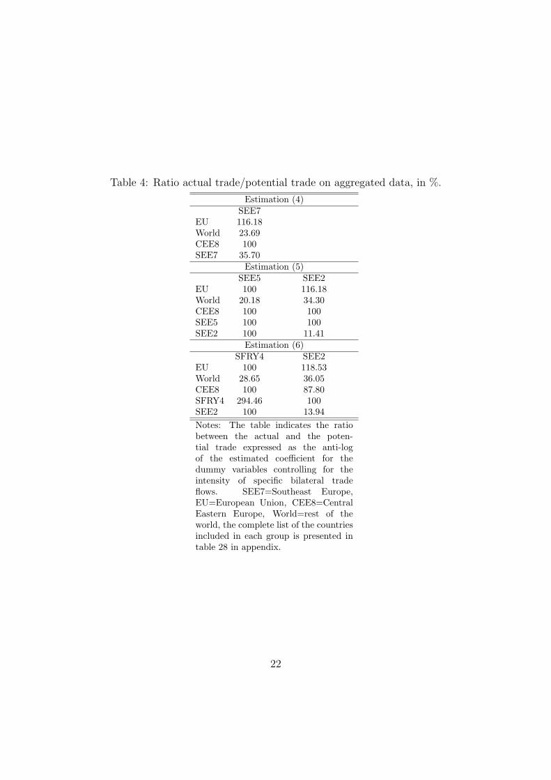
Table 4: Ratio actual trade/potential trade on aggregated data, in %.

Estimation (4)SEE7

EU 116.18World 23.69CEE8 100SEE7 35.70

Estimation (5)SEE5 SEE2

EU 100 116.18World 20.18 34.30CEE8 100 100SEE5 100 100SEE2 100 11.41

Estimation (6)SFRY4 SEE2

EU 100 118.53World 28.65 36.05CEE8 100 87.80SFRY4 294.46 100SEE2 100 13.94Notes: The table indicates the ratiobetween the actual and the poten-tial trade expressed as the anti-logof the estimated coefficient for thedummy variables controlling for theintensity of specific bilateral tradeflows. SEE7=Southeast Europe,EU=European Union, CEE8=CentralEastern Europe, World=rest of theworld, the complete list of the countriesincluded in each group is presented intable 28 in appendix.

22

Western Balkans (Albania, Bosnia-Herzegovina, Croatia, Macedonia and Serbia-

Montenegro) and the Eastern Balkans (Bulgaria and Romania).

Third, the results indicating an intensity lower than the norm for mutual trade

flows of SEE countries. They are higher than 36% of the level predicted by the

model (Table 4, estimation (4)). In the case of mutual trade flows of SEE countries

this result can be surprising since we have shown that there is a high intensity

of trade flows between Successor States of former Yugoslavia. This effect could

actually be explained by the low trade intensity between Bulgaria and Romania and

on the other hand, between countries of the Western part of the Balkan peninsula.

Actually, the first were members of the Council for Mutual Economic Assistance

and reoriented quickly their trade towards the EU after its dissolution.

Fourth, trade flows between SEE countries and the rest of the world represent

only one fourth of their potential (Table 4, estimation (4)). This result can be

compared to those of Babetskaia-Khukarchuk and Maurel (2004) who show that

trade flows of CEE countries and Commonwealth of Independent States (CIS)

countries reach only one third and one fifth of their potential. In the case of SEE

countries the trade deficit with the rest of the world can be partly explained by the

periods of conflicts and sanctions and by their late integration in the international

institutions and notably in the WTO26.

We then try to identify whether the results differ when we separate SEE coun-

tries in two groups, Bulgaria and Romania (Eastern Balkans, SEE2) on one side,

and the four successor states of former Yugoslavia and Albania (Western Balkans,

SEE5) on the other side (Table 5, column 5). The coefficients of the national

incomes, of distance and exchange rate volatility are very close to those estimated

previously. The results obtained for the dummy variables of regional integration

are different from those obtained previously and they confirm the existence of two

sub-regional trade area in SEE.

The results of estimation (5) (Table 5) indicates that the volume of trade of

Western Balkans (SEE5) with the EU does not differ significantly of its predicted

level. The positive and significant coefficient we obtained previously was therefore

due to the intensity of trade between Eastern Balkans(Bulgaria and Romania)

26Subramanian and Wei (2003) show, contrary to Rose (2005), that the WTO had an importantthough uneven impact on trade.

23

Table 5: Results on aggregated data, estimations (5)-(6).Dependent variable: HT HTLn(Imports) (5) (6)Ln(GDPit) 1.47a 1.48a

(0.09) (0.09)Ln(GDPjt) 1.05a 1.00a

(0.08) (0.08)Ln(Distanceij) -1.69a -1.64a

(0.16) (0.20)Volatilityijt -0.15a -0.15a

(0.02) (0.02)SEE5-EU 0.15

(0.10)SEE5-World -1.60a

(0.18)CEE8-SEE5 0.01

(0.31)SEE5-SEE5 0.02

(0.59)SEE2-EU 0.15c 0.17c

(0.09) (0.09)SEE2-World -1.07a -1.02a

(0.18) (0.18)CEE8-SEE2 -0.23 -0.13

(0.39) (0.41)SEE2-SEE2 -2.17c -1.97c

(1.22) (1.29)SEE5-SEE2 0.79

(0.52)SFRY4-EU 0.05

(0.12)SFRY4-World -1.25a

(0.18)CEE8-SFRY4 0.04

(0.35)SFRY4-SFRY4 1.08c

(0.70)SFRY4-SEE2 0.86

(0.56)Nb. of obs. 13143 13143Hausman test 7.79 2.19Prob>Chi2 0.8568 0,9997Notes: a, b and c represent respectively the 1%,5% and 10% significance levels. Standard Er-rors are presented between parenthesis. The coef-ficients of the fixed effects are not reported. Es-timations realized with the Hausman-Taylor model(HTM). SEE7=Southeast Europe, EU=EuropeanUnion, CEE8=Central Eastern Europe, World=restof the world, the complete list of the countries in-cluded in each group is presented in Table (28) inappendix.

24

and the EU. This is confirmed by the estimated coefficient of SEE2− EU which

shows that trade is between 15% and 20% over its potential level. The preferences

granted by the EU to the Western Balkans did not lead, up to now, to trade levels

higher to the norm. However, one can not conclude that they had not effect. One

has to compare them before and after the granting of the preferences. Since the

study covers 1994-2002, the period after the preferences is too short to get reliable

results. However we can have an idea of the potential increase of trade flows

Western Balkans with the EU on the base of the positive and significant coefficient

of the variable SEE2 − EU . The estimated coefficient indicates that trade flows

between Bulgaria and Romania and the EU outreach the norm of 17%. It is

therefore possible that the trade liberalization between the EU and the Western

Balkans (SEE5) will have a similar impact.

The second result induced by this new specification concerns mutual trade be-

tween Western Balkans. It does not differ significantly from its potential, since

the estimated coefficient of SEE5− SEE5 is not significantly different zero. One

can therefore expect a limited impact of the free trade agreements signed at the

beginning of the year 2000. This assumption is reinforced by the fact that mutual

trade preferences of transition countries, like for example the CEFTA, have had

limited effects on trade flows (Dangerfield, 2001). This is confirmed by the coeffi-

cient estimated for the variable indicating trade intensity of mutual trade between

Bulgaria and Romania, which is largely inferior to its potential. This is proba-

bly explained by the important trade reorientation of trade flows towards the EU

which reduced their mutual trade flows. The sectoral analysis of the next section

will refine this result and determine whether trade diversion took place in some

particular sectors.

The other results are not affected by the new specification: trade flows between

SEE and CEE countries do not differ from the norm, and their trade with the rest

of the world is below its potential (Table 5, column 5). However it is interesting

to note that the Western Balkans have a higher trade deficit with the rest of the

world than Bulgaria and Romania, since their trade flows with the rest of the world

represent one fifth of their potential against one third for the two countries of the

Eastern Balkans.

In a second estimation (Table 5, column 6), we exclude Albania from West-

25

ern Balkans, which is composed of the 4 Successor States of former Yugoslavia

(SFRY4). The results are almost not affected except the coefficient of SFRY 4−SFRY 4 which becomes positive and significant, indicating trade flows between

Successor States higher than their potential.

Finally, the results reveal a high geographic concentration of SEE trade flows

with the other European countries. We can expect a low impact of trade liberaliza-

tion between SEE countries but an increase of trade flows between SEE countries

and the EU15 countries on one hand and with the rest of the world on the other

hand. Trade flows with the CEE8 have outreached their potential. A second step

of our work will consist in evaluating the degree of trade integration of SEE coun-

tries, in order to identify if some particular sectors can explain the aggregated

trade patterns.

3.4 Estimations on disaggregated data

The second set of estimates is realized on disaggregated data. We use the 10

sectors classification of the CHELEM-CEPII database27. The results are presented

in Tables 6 and 7. The estimated equation is the same as in the previous section. It

would have been possible to modify the specification so it could fit better the data of

each sector, but it would not allow the comparison of the coefficients estimated for

each sector. The empirical strategy is slightly different in this section. We showed

that SEE is constituted of two sub-regions, the Western and the Eastern Balkans,

which are different by their de jure and de facto trade integration with their main

partners. We therefore evaluate directly the potentials of each region with its main

partners (Table 6). We then exclude Albania of the group of Western Balkans

(Table 7). The evaluations of the trade potentials are presented in Table (8).

The analysis of the estimated coefficients of the gravity variables is interesting

for several reasons. The coefficients of national incomes of the importing countries

are always significant. On the contrary, the estimated coefficients of national

incomes of the exporting countries are not significant for steel and minerals, since

trade does not depend of the economic size of these countries.

27The classification and the content of each sector are available in the appendix, in Tables 29and 30.

26

Tab

le6:

Est

imat

esby

sect

or,es

tim

atio

ns

(7)-

(16)

.

Dep

ende

ntva

riab

le:

Agr

icul

ture

Bas

icm

etal

sC

hem

ical

sC

onst

ruct

ion

Ene

rgy

Met

alpr

oduc

tsM

inin

gTex

tile

sW

ood

pape

rFo

odpr

oduc

tsLn(

Impo

rts)

(7)

(8)

(9)

(10)

(11)

(12)

(13)

(14)

(15)

(16)

Ln(

GD

Pit)

1.33

a1.

25a

1.05

a1.

36a

1.10

a1.

63a

0.97

a1.

05a

1.15

a1.

49a

(0.1

4)(0

.16)

(0.1

1)(0

.13)

(0.2

5)(0

.11)

(0.1

9)(0

.11)

(0.1

1)(0

.12)

Ln(

GD

Pjt)

0.70

a0.

191.

33a

1.00

a0.

59b

1.62

a-0

.20

0.71

a0.

93a

0.60

a

(0.1

2)(0

.15)

(0.0

9)(0

.12)

(0.2

3)(0

.10)

(0.1

7)(0

.10)

(0.1

0)(0

.11)

Ln(

Dis

tanc

e ij)

-2.0

3a-1

.88a

-1.9

6a-2

.53a

-0.3

9-1

.89a

-0.9

4-2

.46a

-1.9

7a-1

.98a

(0.2

9)(0

.40)

(0.2

1)(0

.34)

(0.8

8)(0

.21)

(0.6

1)(0

.25)

(0.2

2)(0

.29)

Vol

atili

tyij

t-0

.03

-0.0

6-0

.06b

-0.0

9a-0

.07

-0.2

2a0.

11b

-0.2

0a-0

.13a

-0.1

0a

(0.0

4)(0

.04)

(0.0

3)(0

.03)

(0.0

6)(0

.03)

(0.0

5)(0

.03)

(0.0

3)(0

.03)

SEE

5-E

U-0

.20

-0.0

9-0

.16

-0.5

0a0.

49-0

.05

-0.0

6-0

.13

0.02

-0.2

7c

(0.1

8)(0

.21)

(0.1

4)(0

.17)

(0.3

7)(0

.13)

(0.2

9)(0

.14)

(0.1

3)(0

.16)

SEE

5-W

orld

-1.2

3a-1

.93a

-1.7

8a-1

.28a

-0.2

7-1

.12a

-2.0

6a-1

.86a

-2.1

1a-0

.92a

(0.2

7)(0

.34)

(0.2

0)(0

.29)

(0.7

7)(0

.22)

(0.5

1)(0

.23)

(0.2

1)(0

.27)

SEE

5-C

EE

8-0

.26

-0.4

5-0

.00

-0.5

21.

250.

36-0

.08

-1.8

2a-0

.17

-0.1

3(0

.51)

(0.6

5)(0

.38)

(0.5

5)(0

.97)

(0.4

0)(0

.85)

(0.4

5)(0

.39)

(0.5

1)SE

E5-

SEE

5-0

.41

-1.9

6c-0

.74

-0.8

52.

960.

98-1

.60

-3.9

0a-2

.18a

-0.4

2(0

.93)

(1.1

7)(0

.69)

(1.0

1)(2

.13)

(0.7

5)(1

.56)

(0.8

2)(0

.73)

(0.9

4)SE

E2-

EU

-0.5

0a-0

.09

0.56

a-0

.27

0.47

0.31

c0.

360.

110.

29c

-0.0

3(0

.19)

(0.2

1)(0

.15)

(0.1

7)(0

.36)

(0.1

6)(0

.29)

(0.1

6)(0

.15)

(0.1

7)SE

E2-

Wor

ld-1

.00a

-0.8

1a-1

.53a

-0.9

4a-0

.42

-1.3

3a-0

.95b

-0.7

5a-1

.45a

-1.0

4a

(0.2

6)(0

.31)

(0.2

0)(0

.27)

(0.4

9)(0

.22)

(0.3

8)(0

.24)

(0.2

1)(0

.28)

SEE

2-C

EE

8-1

.06c

-1.5

4b0.

24-0

.82

0.21

0.53

-1.3

7-2

.04a

-0.9

4b-0

.17

(0.5

8)(0

.71)

(0.4

4)(0

.62)

(1.0

6)(0

.49)

(0.9

3)(0

.54)

(0.4

7)(0

.62)

SEE

2-SE

E2

-2.7

6-1

.93

-2.0

6-3

.86b

3.09

-2.6

6c0.

19-5

.04a

-3.6

6b-2

.64

(1.7

8)(2

.15)

(1.3

4)(1

.89)

(3.0

8)(1

.52)

(2.5

8)(1

.68)

(1.4

5)(1

.94)

SEE

5-SE

E2

-0.0

3-0

.03

0.98

c-0

.35

2.10

0.63

0.96

-2.4

4a-0

.05

-0.4

9(0

.76)

(0.9

3)(0

.58)

(0.8

2)(1

.31)

(0.6

5)(1

.14)

(0.7

1)(0

.62)

(0.8

1)N

b.of

obs.

1197

111

357

1251

211

443

9253

1285

499

1512

578

1252

312

271

Hau

sman

test

6.94

29.9

47.

564.

553.

106.

126.

7521

.13

4.36

7.46

Pro

b>C

hi2

0.86

190.

0000

0.87

130.

9840

0.99

480.

8812

0.87

400.

0000

0.98

670.

8768

Not

es:

a,

ban

dc

repr

esen

tre

spec

tive

lyth

e1%

,5%

and

10%

sign

ifica

nce

leve

ls.

Stan

dard

Err

ors

are

pres

ente

dbe

twee

npa

rent

hesi

s.T

heco

effici

ents

ofth

efix

edeff

ects

are

not

repo

rted

.E

stim

atio

nsre

aliz

edw

ith

the

Hau

sman

-Tay

lor

mod

el(H

TM

).SE

E7=

Sout

heas

tE

urop

e,E

U=

Eur

opea

nU

nion

,C

EE

8=C

entr

alE

aste

rnE

urop

e,W

orld

=re

stof

the

wor

ld,

the

com

plet

elis

tof

the

coun

trie

sin

clud

edin

each

grou

pis

pres

ente

din

tabl

e28

inap

pend

ix.

The

prod

ucts

incl

uded

inea

chse

ctor

are

pres

ente

din

tabl

es29

and

30.

27

The results obtained for the distance variable, which in our specification is

a proxy for trade costs, are also interesting. All the estimated coefficients are

negative, which is consistent with our expectations, but the estimated coefficients

for energy and minerals are not significant. It seems to indicate that distance is

not a good proxy for trade costs in these sectors. For what concerns the other

coefficients, it is surprising that the two highest coefficients in absolute terms are

obtained for construction goods and textile products. Construction goods are

heavier, which justifies higher transportation costs, but this explanation is not

valid for textile. A plausible explanation is that distance does not only capture

transportation costs but also other barriers to trade. Trade of textile goods is often

regulated by special treatments28.

The impact of exchange rate volatility varies according to the sectors, it is neg-

ative for all sectors except for minerals and it is almost always significant. These

results are consistent with those of Peridy (2003), who shows that the relation-

ship between trade and exchange rate volatility depends of the characteristics of

particular firms or markets and that there is a sectoral and geographic bias in the

estimations on aggregated data. The results indicate that the negative impact of

the exchange rate volatility is higher on the trade of higher value added goods.

Thus, the highest coefficients in absolute terms are observed for the mechanics and

for textile. On the contrary it is not significantly different from 0 for agricultural

goods, steel, energy and it is positive for minerals.

The analysis of the coefficients of the variables of regional trade integration

by sector also lead to interesting results, which tend to confirm those obtained on

aggregated data. The ratios are presented in Table (8). Thus the trade flows of

SEE countries with the rest of the world differ significantly from their potentials for

all sectors (Tables ??? 10a. and b.). It is the trend we identified on aggregated

data.

However, some sectors are somewhat different of the global trend. Thus it

appears that the volume of trade in sectors such as construction and food products

of SEE5 with the EU represent respectively two third and three quarters of their

potential (Table ??? 10a.). For all other products trade does not differ from the

28Imports of textile products of industrialized countries have been limited from 1974 to 2004by the Multifiber Agreement.

28

norm. For trade flows with the rest of the world it is the sector of energy which is

different from the general trend. For this sector almost all the ratios are equal to

100%. A plausible explanation is that proximity and formal regional integration

have a rather limited explanatory power of the volume of trade.

If we look at the trade potential of the SEE5 countries with the CEE countries

in the textile it appears clearly that it is not reached, since it represents only 16%

of its potential (Table ??? 10a.). For the other sector the potential is reached.

Actually, this trend can be observed for the mutual trade flows of SEE countries

and between them and the CEE. On the contrary, the volume of trade with the EU

has reached its potential. A plausible explanation for this result is that trade in

textile has been largely reoriented towards the EU, notably through outward trade

process. Andreff et alii (2001) have shown that this kind of trade between CEE

and the EU has been quite important in the textile during the 1990s. Moreover,

this result is close to Fukao et alii (2003), who show that NAFTA has diverted

more trade in the textile sector. The mutual trade flows between Western Balkan

countries in the wood sector is also lower than its potential. Once again, trade

diversion with EU countries can constitute a plausible explanation.

The analysis of the results for the Eastern Balkans countries (Bulgaria and

Romania) first indicates that agriculture is the only sector in which trade flows with

the EU are lower than their potential, they represent only 60% of it (Table ???

10b.). A possible explanation is that agricultural goods have been initially excluded

from the association agreements. However, textile goods and chemicals have also

been initially excluded and, in these sectors, trade with the EU have reached their

potential. Moreover, the potential is reached with the Western Balkans. This result

could therefore reflect the low productivity of this sector and/or the low quality

of the products, which tend to reduce trade flows with the EU. In the sectors of

mechanics, wood, and chemicals, the potential is outreached from 36% to 75%

(Table ??? 10b.), which can reflect the effect of preferential trade agreements.

If we have a look at the trade flows of Eastern Balkans with the rest of the world

we observe the sector of energy is the only one for which the real trade is higher

than the norm. This is not surprising since, on one hand the determinants of trade

in this sector differ from the other sectors and on the other hand Bulgaria has

inherited from the Council of Mutual Economic Assistance a specialization in the

29

refining of the Russian oil. Finally an interesting result is that trade flows between

Bulgaria and Romania are much lower than than their potential in all sectors,

except energy, minerals and food products. Two complementary explanations are

possible. First, there was a strong trade reorientation towards the EU in most of

the sectors, and second, this result could reflect the heritage of the trade patterns

within the CMEA29.

The results obtained when we exclude Albania from the group of the Western

Balkans are presented in Table 7. The ratios between the real and the potential

trade flows are presented in Table 8c. These new results differ only slightly from the

previous. We observe that trade potentials are not reached between the Successor

States of former Yugoslavia (SFRY4) for steel (30% of the potential), and textile

(7% of the potential). On the other hand, the potential is largely outreached in

the sectors of mechanical goods since trade flows are 9 times higher to the norm.

The potentials estimated for the Eastern Balkans (SEE2) differ only slightly with

this new specification.

29In the CMEA (1949-1991), Romania and Bulgaria traded essentially with the USSR andvery few between themselves. Trade patterns could be compared to a star, with USSR at thecenter (Graziani, 1981).

30

Tab

le7:

Est

imat

esby

sect

or,es

tim

atio

ns

(17)

-(26

).

Dep

ende

ntva

riab

le:

Agr

icul

ture

Bas

icm

etal

sC

hem

ical

sC

onst

ruct

ion

Ene

rgy

Met

alpr

oduc

tsM

inin

gTex

tile

sW

ood

pape

rFo

odpr

oduc

tsLn(

Impo

rts)

(17)

(18)

(19)

(20)

(21)

(22)

(23)

(24)

(25)

(26)

Ln(

GD

Pit)

1.33

a1.

26a

1.05

a1.

35a

1.09

a1.

64a

1.00

a1.

06a

1.15

a1.

48a

(0.1

4)(0

.16)

(0.1

0)(0

.12)

(0.2

5)(0

.11)

(0.1

9)(0

.11)

(0.1

1)(0

.12)

Ln(

GD

Pjt)

0.68

a0.

151.

28a

0.98

a0.

57b

1.58

a-0

.22

0.66

a0.

89a

0.58

a

(0.1

2)(0

.15)

(0.0

9)(0

.12)

(0.2

3)(0

.10)

(0.1

7)(0

.11)

(0.1

0)(0

.11)

Ln(

Dis

tanc

e ij)

-1.9

2a-2

.03a

-2.0

9a-2

.77a

0.50

-1.7

0a-0

.54

-2.7

4a-2

.10a

-2.1

2a

(0.3

7)(0

.55)

(0.2

7)(0

.48)

(1.5

4)(0

.26)

(0.8

8)(0

.34)

(0.2

8)(0

.38)

Vol

atili

tyij

t-0

.03

-0.0

6-0

.06b

-0.1

0a-0

.08

-0.2

2a0.

11b

-0.2

0a-0

.13a

-0.1

0a

(0.0

4)(0

.04)

(0.0

3)(0

.03)

(0.0

6)(0

.03)

(0.0

5)(0

.03)

(0.0

3)(0

.03)

SFRY

4-E

U-0

.12

0.12

-0.2

0-0

.55a

0.26

0.06

0.05

-0.0

60.

09-0

.43b

(0.2

0)(0

.23)

(0.1

5)(0

.19)

(0.3

9)(0

.15)

(0.3

0)(0

.16)

(0.1

5)(0

.17)

SFRY

4-W

orld

-1.1

4a-2

.06a

-1.5

8a-1

.36a

0.66

-0.8

5a-1

.70b

-1.9

2a-1

.98a

-0.8

5a

(0.3

0)(0

.42)

(0.2

2)(0

.36)

(1.2

9)(0

.23)

(0.7

4)(0

.27)

(0.2

3)(0

.31)

SFRY

4-C

EE

8-0

.05

-0.2

1-0

.10

-0.7

41.

720.

630.

43-1

.76a

-0.2

4-0

.25

(0.5

9)(0

.82)

(0.4

5)(0

.70)

(1.2

8)(0

.45)

(1.0

2)(0

.57)

(0.4

8)(0

.60)

SFRY

4-SF

RY

40.

96-1

.23

0.13

-0.5

65.

162.

14b

-0.1

1-2

.68b

-1.1

80.

43(1

.15)

(1.5

4)(0

.86)

(1.3

5)(3

.46)

(0.8

9)(2

.14)

(1.1

1)(0

.93)

(1.2

1)SE

E2-

EU

-0.4

7b-0

.07

0.56

a-0

.28c

0.51

0.35

b0.

460.

110.

30b

-0.0

3(0

.19)

(0.2

2)(0

.15)

(0.1

7)(0

.37)

(0.1

6)(0

.30)

(0.1

6)(0

.15)

(0.1

7)SE

E2-

Wor

ld-0

.98a

-0.8

7a-1

.50a

-0.9

6a-0

.07

-1.2

8a-0

.97b

-0.8

2a-1

.46a

-1.0

8a

(0.2

6)(0

.34)

(0.2

0)(0

.30)

(0.6

7)(0

.21)

(0.4

1)(0

.27)

(0.2

3)(0

.29)

SEE

2-C

EE

8-0

.93

-1.5

9b0.

15-1

.04

0.67

0.73

-0.8

6-2

.14a

-0.9

6c-0

.25

(0.6

1)(0

.80)

(0.4

8)(0

.73)

(1.3

7)(0

.50)

(1.0

8)(0

.62)

(0.5

2)(0

.67)

SEE

2-SE

E2

-2.4

6-2

.22

-2.2

7-4

.38b

4.97

-2.1

71.

15-5

.56a

-3.8

6b-2

.93

(1.8

4)(2

.44)

(1.4

8)(2

.20)

(4.2

6)(1

.54)

(2.9

7)(1

.96)

(1.6

3)(2

.09)

SFRY

4-SE

E2

0.13

0.21

0.88

-0.8

52.

390.

932.

09-2

.48a

-0.0

1-0

.63

(0.8

5)(1

.10)

(0.6

9)(1

.00)

(1.6

4)(0

.71)

(1.3

0)(0

.89)

(0.7

4)(0

.94)

Nb.

ofob

s.11

971

1135

712

512

1144

392

5312

854

9915

1257

812

523

1227

1H

ausm

ante

st1.

230.

490.

783.

991.

863.

086.

932.

338.

053.

05P

rob>

Chi

21.

0000

1.00

001.

0000

0.98

010.

9996

0.98

900.

8072

0.99

820.

8512

0.99

52N

otes

:a,

ban

dc

repr

esen

tre

spec

tive

lyth

e1%

,5%

and

10%

sign

ifica

nce

leve

ls.

Stan

dard

Err

ors

are

pres

ente

dbe

twee

npa

rent

hesi

s.T

heco

effici

ents

ofth

efix

edeff

ects

are

not

repo

rted

.E

stim

atio

nsre

aliz

edw

ith

the

Hau

sman

-Tay

lor

mod

el(H

TM

).SE

E7=

Sout

heas

tE

urop

e,E

U=

Eur

opea

nU

nion

,C

EE

8=C

entr

alE

aste

rnE

urop

e,W

orld

=re

stof

the

wor

ld,

the

com

plet

elis

tof

the

coun

trie

sin

clud

edin

each

grou

pis

pres

ente

din

Tab

le(2

8)in

appe

ndix

.T

hepr

oduc

tsin

clud

edin

each

sect

orar

epr

esen

ted

inTab

les

29an

d30

.

31

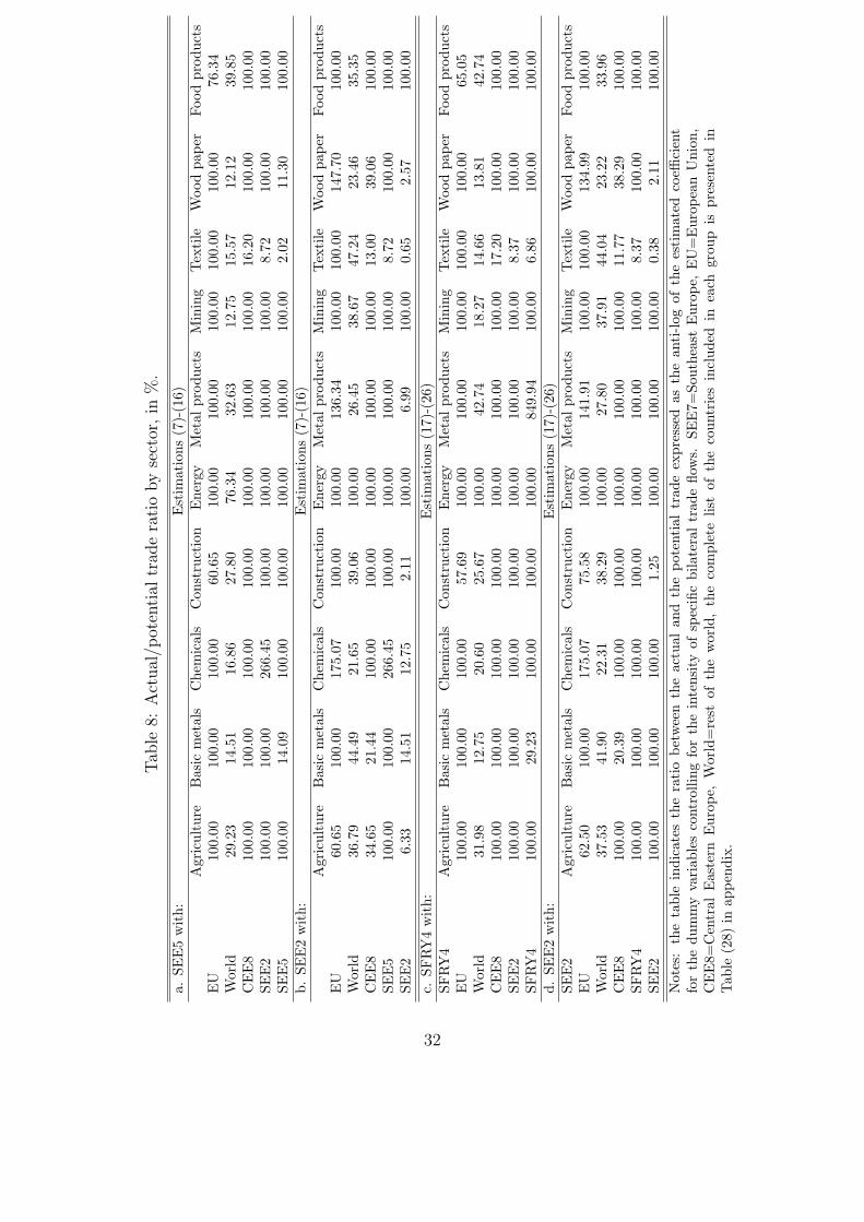
Tab

le8:

Act

ual

/pot

ential

trad

era

tio

by

sect

or,in

%.

a.SE

E5

with:

Est

imat

ions

(7)-

(16)

Agr

icul

ture

Bas

icm

etal

sC

hem

ical

sC

onst

ruct

ion

Ene

rgy

Met

alpr

oduc

tsM

inin

gTex

tile

Woo

dpa

per

Food

prod

ucts

EU

100.

0010

0.00

100.

0060

.65

100.

0010

0.00

100.

0010

0.00

100.

0076

.34

Wor

ld29

.23

14.5

116

.86

27.8

076

.34

32.6

312

.75

15.5

712

.12

39.8

5C

EE

810

0.00

100.

0010

0.00

100.

0010

0.00

100.

0010

0.00

16.2

010

0.00

100.

00SE

E2

100.

0010

0.00

266.

4510

0.00

100.

0010

0.00

100.

008.

7210

0.00

100.

00SE

E5

100.

0014

.09

100.

0010

0.00

100.

0010

0.00

100.

002.

0211

.30

100.

00b.

SEE

2w

ith:

Est

imat

ions

(7)-

(16)

Agr

icul

ture

Bas

icm

etal

sC

hem

ical

sC

onst

ruct

ion

Ene

rgy

Met

alpr

oduc

tsM

inin

gTex

tile

Woo

dpa

per

Food

prod

ucts

EU

60.6

510

0.00

175.

0710

0.00

100.

0013

6.34

100.

0010

0.00

147.

7010

0.00

Wor

ld36

.79

44.4

921

.65

39.0

610

0.00

26.4

538

.67

47.2

423

.46

35.3

5C

EE

834

.65

21.4

410

0.00

100.

0010

0.00

100.

0010

0.00

13.0

039

.06

100.

00SE

E5

100.

0010

0.00

266.

4510

0.00

100.

0010

0.00

100.

008.

7210

0.00

100.

00SE

E2

6.33

14.5

112

.75

2.11

100.

006.

9910

0.00

0.65

2.57

100.

00c.

SFRY

4w

ith:

Est

imat

ions

(17)

-(26

)SF

RY

4A

gric

ultu

reB

asic

met

als

Che

mic

als

Con

stru

ctio

nE

nerg

yM

etal

prod

ucts

Min

ing

Tex

tile

Woo

dpa

per

Food

prod

ucts

EU

100.

0010

0.00

100.

0057

.69

100.

0010

0.00

100.

0010

0.00

100.

0065

.05

Wor

ld31

.98

12.7

520

.60

25.6

710

0.00

42.7

418

.27

14.6

613

.81

42.7

4C

EE

810

0.00

100.

0010

0.00

100.

0010

0.00

100.

0010

0.00

17.2

010

0.00

100.

00SE

E2

100.

0010

0.00

100.

0010

0.00

100.

0010

0.00

100.

008.

3710

0.00

100.

00SF

RY

410

0.00

29.2

310

0.00

100.

0010

0.00

849.

9410

0.00

6.86

100.

0010

0.00

d.SE

E2

with:

Est

imat

ions

(17)

-(26

)SE

E2

Agr

icul

ture

Bas

icm

etal

sC

hem

ical

sC

onst

ruct

ion

Ene

rgy

Met

alpr

oduc

tsM

inin

gTex

tile

Woo

dpa

per

Food

prod

ucts

EU

62.5

010

0.00

175.

0775

.58

100.

0014

1.91

100.

0010

0.00

134.

9910

0.00

Wor

ld37

.53

41.9

022

.31

38.2

910

0.00

27.8

037

.91

44.0

423

.22

33.9

6C

EE

810

0.00

20.3

910

0.00

100.

0010

0.00

100.

0010

0.00

11.7

738

.29

100.

00SF

RY

410

0.00

100.

0010

0.00

100.

0010

0.00

100.

0010

0.00

8.37

100.

0010

0.00

SEE

210

0.00

100.

0010

0.00

1.25

100.

0010

0.00

100.

000.

382.

1110

0.00

Not

es:

the

tabl

ein

dica

tes

the

ratio

betw

een

the

actu

alan

dth

epo

tent

ial

trad

eex

pres

sed

asth

ean

ti-log

ofth

ees

tim

ated

coeffi

cien

tfo

rth

edu

mm

yva

riab

les

cont

rolli

ngfo

rth

ein

tens

ity

ofsp

ecifi

cbi

late

ral

trad

eflo

ws.

SEE

7=So

uthe

ast

Eur

ope,

EU

=E

urop

ean

Uni

on,

CE

E8=

Cen

tral

Eas

tern

Eur

ope,

Wor

ld=

rest

ofth

ew

orld

,th

eco

mpl

ete

list

ofth

eco

untr

ies

incl

uded

inea

chgr

oup

ispr

esen

ted

inTab

le(2

8)in

appe

ndix

.

32

4 The impact of trade liberalization on trade

flows

In this section we evaluate the impact of trade liberalization on manufactured

trade of Balkan countries. We analyze this question at the sectoral level and focus

on exports flows of manufactured goods of Balkan countries all over the world30.

We also use data on bilateral tariff barriers (TBs) and nontariff barriers (NTBs)

to trade. Due to some data constraints, we focus on 7 manufactured sectors31, on

the period 1996-2000 and we retain 6 Balkan countries32.

We find that exports are increasing in all sectors during the period, while

bilateral tariffs are decreasing. However, this liberalization process exhibits small

effects on trade. Actually, we find small but significant estimates of the impact of

trade liberalization on Balkan countries’ exports. Other things being equal, a one

point decrease of bilateral tariffs increases exports from 2.2% to 8.6% according to

the sector. These findings are mostly in line with the existing literature, pointing

out that “effects on trade (. . .) are likely to be small” (Deardoff and Stern, 1986).

We find that, if tariffs are decreasing, nontariff barriers are increasing during

the period. Trade liberalization should not be treated as a given (Trefler, 1993).

Domestic firms, competiting with Balkan exporters, may have increased their lob-

bying activity for greater protection. As a result, NTBs increase and hurt exports

from Balkan countries. In that respect, we find large estimates of NTBs on ex-

ports in 4 out of our 7 sectors (textile, wood and paper, construction and metal

products)33. A one point decrease of NTBs increases exports from 67% to 227%.

The rest of this section is organized as follows. We first present some descriptive

statistics. Then, we present our estimation strategy which is slightly different from

the preceding sections. Finally, we report our results and present a summary of

the estimates of TBs and NTBs on trade.

30We previously used imports at the sectoral level, but we face some data constraints. Ouravailable information on bilateral tariff and nontariff variables is related to exports of Balkancountries

31Food, textile, wood and paper, chemical, construction, basic metal and metal products, seeTables (29) and (30) in appendix for details.

32Bosnia-Herzegovina, Bulgaria, Croatia, Macedonia, Romania and Slovenia.33The estimates of NTBs in the other sectors are not significantly different from zero.

33

4.1 Basic statistics

Exports

Sectoral exports of Balkan countries all over the world come from CEPII34 .

The sample covers 1996-2000. During this period, exports are increasing in almost

all sectors such as textile (+3.3% in log terms between 1996 and 2000), metal

products (+2.4%), basic metal (+2%), wood and Paper (+1.9%) and construction

(+1,3%)]. Exports are rather stable in chemical industry (+0.5%) and decreasing

in food industry (-1.7%) (see Figure 1). Interestingly, we observe that all sectors

experienced a drop in 1999. This maybe explained by the upsurge of uncertainty

in the region due to the bombing on Serbia.

67

89

67

89

67

89

1996 1997 1998 1999 20001996 1997 1998 1999 2000

1996 1997 1998 1999 2000

Basic Metal Chemical Construction

Fabricated Metal Food Textile

Wood and Paper

Log

of to

tal o

f bila

tera

l exp

orts

yearSource: Authors’ computation, (TRAINS, CEPII)

by sectors, 1996−2000Bilateral exports of Balkan countries

Figure 1: Bilateral exports of Balkan countries, by sector, 1996-2000.

34All the main importing partners are retained. See Table (28) in appendix for a list of coun-tries. Mayer and Zignago (2005) and the CEPII website (http://www.cepii.fr) provide additionaldetails.

34

Bilateral tariff barriers on trade

The TRAINS database developed by the UNCTAD offers the most complete

data available on policy barriers to trade (Anderson and van Wincoop, 2004).

TRAINS reports data on bilateral tariffs for roughly 5000 “products”. Using this

data, Jon Haveman computes weighted averages of bilateral tariffs35, which are

retreated and published on the CEPII website36 (Mayer and Zignago, 2005).

Due to the substantial incompleteness of TRAINS37 our measure of tariff is

rather crude. We can however draw several lessons from it (see Figure 2). Tariffs

are sharply increasing in 1997 and decreasing since there in all sectors.

010

2030

010

2030

010

2030

1996 1997 1998 1999 20001996 1997 1998 1999 2000

1996 1997 1998 1999 2000

Basic Metal Chemical Construction

Fabricated Metal Food Textile

Wood and Paper

Sim

ple

aver

age

of b

ilate

ral t

ariff

bar

riers

(in

%)

yearSource: Authors’ computation, (TRAINS, CEPII)

by sectors, 1996−2000Bilateral tariff barriers on Balkan countries exports

Figure 2: Bilateral tariff barriers on Balkan countries’ exports, by sector, 1996-2000.

35See the Ultimate Trade Barrier Catalog at http://www.eiit.org/Protection.36See http://www.cepii.fr.37See Table (1) in Anderson and van Wincoop, 2004.

35

0.2

.4.6

.80

.2.4

.6.8

0.2

.4.6

.8

1996 1997 1998 1999 20001996 1997 1998 1999 2000

1996 1997 1998 1999 2000

Basic Metal Chemical Construction

Fabricated Metal Food Textile

Wood and Paper

Sim

ple

aver

age

of b

ilate

ral n

onta

riff b

arrie

rs (

in %

)

yearSource: Authors’ computation, (TRAINS, CEPII)

by sectors, 1996−2000Bilateral nontariff barriers on Balkan countries exports

Figure 3: Bilateral nontariff barriers on Balkan countries’ exports, by sector, 1996-2000.

36

Bilateral nontariff barriers on trade

Bilateral nontariff barriers on trade are also extracted from TRAINS and made

public by the CEPII. These NTBs take different forms, “from traditional bor-

der formalities and administrative harassment to more sophisticated sanitary and

physo-sanitary measures” (Mayer and Zignago, 2005). For a given sector, we use

a frequency index of NTBs varying from 0 to 1 when all the tariff lines of the

underlying sector is subject to a NTB.

This variable also represents an incomplete measure of protection, but offers

some useful insights. During the period 1996-2000, NTBs are increasing in all

sectors (see Figure 3). In some extent, the decrease of TB are compensated by an

increase of NTBs.

4.2 Empirical model

We retain a gravity equation to investigate the impact of trade liberalization on

exports. We use a slightly different equation compared to the preceding sections.

We use the ordinary least squares (OLS) method38 and estimate:

Ln(Exportsijt) = β0 + β1Ln(GDPit) + β2Ln(GDPjt) + β3Ln(Distanceijt)

+β4Tariffijt + β5Ntbijt +∑

(βlZlijt)

+φtIt + εijt, (2)

where i denotes the destination country and j the source country. The variables

are defined as follows:

• (Exportsij) is the value of manufactured exports between i and j;

• (GDP ) is the Gross Domestic Product;

• (Distanceij) denotes the distance between i and j;

• (Tariffij) is the bilateral sector-level tariff barriers on exports from i to j (in

percent);

38We depart from the Hausman-Taylor estimator since the simplest OLS method suits well ourpurposes.

37

• (Ntbij) is a frequency index of bilateral nontariff barriers on exports from i

to j;

• Zlij represents a set of dummy variables capturing various determinants of

bilateral trade, such as:

contiguityij, a dummy variable equals to one if i and j share a border;

samecountryij, a dummy variable equals to one if i and j were or are

part of the same country;

associationij, a dummy variable equals to one if i and j share an associ-

ation agreement with the EU;

• (It) is a vector of year dummies that take a value of one in year t for t =

1, . . . , T ;

• (εij) is an error term, reflecting measurement error in trade.

4.3 Results

Tariff barriers

We first estimate a shorter version of equation (2), without NTBs and Z vari-

ables. The results are reported in Table (9). It can be seen that our simple model

has considerable explanatory power, except for the Food industry. As expected,

the elasticities of exports with respect to own GDP and importing country-GDP

are positive. Furthermore, the elasticities of distance are negative, indicating that,

other things being equal, an increase of bilateral distance has a negative impact

on trade.

We find small but significant estimates of the impact of trade liberalization on

exports, except for food industry (p<0.1). The estimated coefficients of the tariff

variable are negative, it means that, other things being equal, a one point decrease

of bilateral tariffs increases exports from 2.2% (Construction) to 8.6% (Wood and

Paper)39.

39In a log-level model, the semi-elasticity is interpreted as dy = (100∗betaj)dx (see Woolridge,2003, p.45).

38

Table 9: Tariff barriers estimatesDependant variables: Ln(Exportsij)

Sectors: Food Textile Wood & Chemical Construction Basic MetalPaper Metal Products

Ln(GDPi) 0.727a 0.831a 0.824a 1.020a 0.565a 0.903a 0.972a

(0.088) (0.071) (0.051) (0.060) (0.059) (0.065) (0.057)Ln(GDPj) 0.641a 1.009a 0.807a 1.047a 0.710a 0.716a 1.200a

(0.064) (0.046) (0.037) (0.041) (0.041) (0.045) (0.036)Ln(Distanceij) -1.121a -1.697a -1.650a -1.913a -1.520a -1.721a -1.806a

(0.071) (0.060) (0.041) (0.050) (0.050) (0.054) (0.049)Tariffij -0.003c -0.024a -0.086a -0.024b -0.022a -0.028b -0.058a

(0.001) (0.007) (0.007) (0.011) (0.006) (0.012) (0.010)Year fixed effects Yes Yes Yes Yes Yes Yes YesR2 0.37 0.68 0.81 0.78 0.68 0.68 0.82# observations 721 719 722 721 718 721 722Notes: a, b and c define 1%, 5% and 10% significance levels respectively. Heteroskedastic-consistent(White-robust) standard errors are in parentheses. Coefficients for year fixed effects and constant arenot reported. Estimations of equation (2) without the ntb and Z variables.

If we restrict the sample to the exports of Balkan countries to the European

Union countries, we find larger estimates. They however maybe less reliable be-

cause the sample retains only 280 observations. In this case, other things being

equal, a one point decrease of bilateral tariffs significantly increases exports by 56%

in the wood and paper sector, 24% in the construction and 17% in the fabricated

metal industry.

In the previous estimates, we used GDPs to get an approximation of the pro-

duction sector elasticities. It seems more convenient to use directly production by

sectors. We face however some data constraints on this variable which reduces the

available information. Results are reported in Table (10).

Results are in line with the preceding estimates. Thus, coefficients for Wood

and Paper, Chemical and Construction are not statistically different. Only the

estimate for the Textile industry is statistically higher. The coefficients for the

other sectors are not statistically significant, this may be due to the huge drop in

the number of observations.

Nontariff barriers

We now introduce the role of NTBs variable. The results are reported in Ta-

ble (11).

39

Table 10: Tariff barriers estimates including production by sectors

Dependant variables: Ln(Exportsij)Sectors: Food Textile Wood & Chemical Construction Basic Metal

Paper Metal ProductsLn(Productioni) 0.447a 0.508a 0.969a 0.469a 0.603a 0.923a 1.184a

(0.140) (0.067) (0.119) (0.041) (0.101) (0.283) (0.215)Ln(Productionj) 0.770a 1.042a 0.692a 1.020a 0.742a 0.685a 1.008a

(0.102) (0.046) (0.042) (0.045) (0.051) (0.097) (0.037)Ln(Distanceij) -1.175a -1.775a -1.668a -2.013a -1.534a -1.850a -1.788a

(0.133) (0.098) (0.065) (0.073) (0.081) (0.215) (0.081)Tariffij -0.003 -0.054a -0.073a -0.032b -0.024a -0.034 -0.025c

(0.004) (0.010) (0.014) (0.016) (0.009) (0.045) (0.015)Year fixed effects Yes Yes Yes Yes Yes Yes YesR2 0.35 0.73 0.78 0.90 0.69 0.68 0.85# observations 260 338 337 342 333 80 255Notes: a, b and c define 1%, 5% and 10% significance levels respectively. Heteroskedastic-consistent(White-robust) standard errors are in parentheses. Coefficients for year fixed effects and constant arenot reported. Estimations of equation (2) without the ntb and Z variables.

Table 11: Nontariff and tariff barriers estimatesDependant variables: Ln(Exportsij)

Sectors: Food Textile Wood & Chemical Construction Basic MetalPaper Metal Products

Ln(GDPi) 0.695a 0.787a 0.791a 1.005a 0.517a 0.879a 0.905a

(0.128) (0.100) (0.077) (0.088) (0.086) (0.094) (0.087)Ln(GDPj) 0.678a 1.078a 0.865a 1.007a 0.741a 0.749a 1.215a

(0.102) (0.062) (0.055) (0.061) (0.058) (0.067) (0.055)Ln(Distanceij) -0.982a -1.487a -1.622a -1.871a -1.522a -1.768a -1.762a

(0.114) (0.105) (0.073) (0.086) (0.086) (0.090) (0.088)Tariffij -0.017b -0.059a -0.084a 0.005 -0.031b -0.015 -0.026

(0.004) (0.013) (0.015) (0.021) (0.015) (0.045) (0.018)Nontariffij 0.886c -0.667b -0.496 -0.026 -0.793 0.784 -1.490a

(0.496) (0.313) (0.343) (0.433) (0.963) (0.500) (0.439)Year fixed effects Yes Yes Yes Yes Yes Yes YesR2 0.36 0.73 0.81 0.79 0.69 0.70 0.83# observations 346 347 347 346 345 347 347Notes: a, b and c define 1%, 5% and 10% significance levels respectively. Heteroskedastic-consistent(White-robust) standard errors are in parentheses. Coefficients for year fixed effects and constant arenot reported. Estimations of equation (2) without the Z variables.

40

The results are quite disappointing due to some sample problems. Introducing

the NTB variable leads to a decrease of the number of observations and to a mul-

ticollinearity problem. The correlation between TB and NTB causes the model to

become unsatisfactory. In Chemical, Construction and Fabricated Metal the pair-

wise correlation coefficients are significant and respectively equal to 0.34, 0.50 and

0.44. This simple correlation is even higher for some specific years. Consequently,

compared to our first estimates [Table (9)], the standard errors are larger when

we introduce the NTBs and some semi-elasticities of the tariff variable become

insignificant.

Estimates in the Textile and the Fabricated Metal industries are however in-

formative. It seems that the effect of NTBs on trade are larger than the impact

of TBs. Other things being equal, a one point decrease of NTBs increases exports

respectively by 67% and 149%.

We now drop the tariffij variable to avoid any multicollinearity problem. The

results are reported in Table (12).

Table 12: Nontariff barriers estimatesDependant variables: Ln(Exportsij)

Sectors: Food Textile Wood & Chemical Construction Basic MetalPaper Metal Products

Ln(GDPi) 0.731a 0.845a 0.471a 1.044a 0.514a 0.839a 0.903a

(0.119) (0.092) (0.080) (0.084) (0.080) (0.087) (0.085)Ln(GDPj) 0.844a 1.127a 1.059a 1.138a 0.806a 0.806a 1.356a

(0.069) (0.053) (0.046) (0.050) (0.046) (0.054) (0.049)Ln(Distanceij) -0.963a -1.631a -1.719a -1.849a -1.508a -1.738a -1.709a

(0.105) (0.082) (0.066) (0.074) (0.074) (0.074) (0.077)Nontariffij 0.769c -0.669a -1.041a 0.173 -1.604b 0.725 -2.272a

(0.435) (0.290) (0.412) (0.397) (0.693) (0.467) (0.418)Year fixed effects Yes Yes Yes Yes Yes Yes YesR2 0.38 0.70 0.75 0.76 0.66 0.68 0.79# observations 411 411 411 411 411 411 411Notes: a, b and c define 1%, 5% and 10% significance levels respectively. Heteroskedastic-consistent(White-robust) standard errors are in parentheses. Coefficients for year fixed effects and constant arenot reported. Estimations of equation (2) without the tariff and Z variables.

They confirm the strong impact of the nontariff barriers on exports of Textile

and Fabricated Metal. Interestingly, we also find large effects in Wood and Paper

and Construction sectors. Other things being equal, a one point decrease of NTBs

41

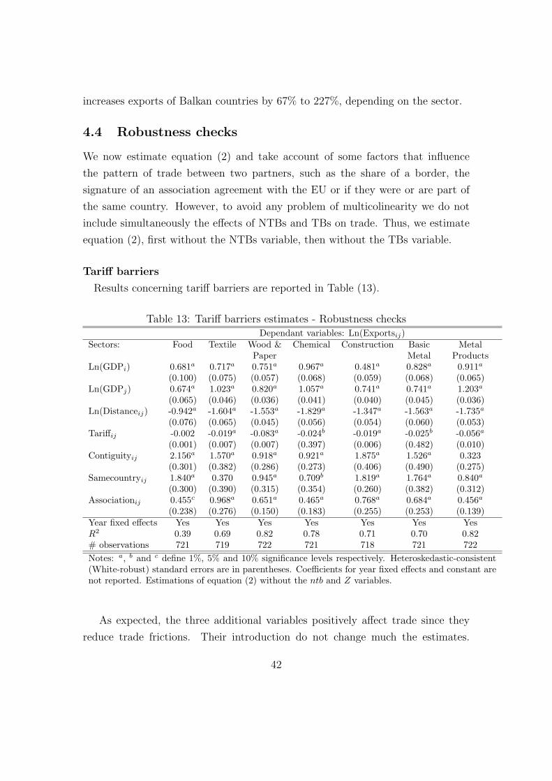
increases exports of Balkan countries by 67% to 227%, depending on the sector.

4.4 Robustness checks

We now estimate equation (2) and take account of some factors that influence

the pattern of trade between two partners, such as the share of a border, the

signature of an association agreement with the EU or if they were or are part of

the same country. However, to avoid any problem of multicolinearity we do not

include simultaneously the effects of NTBs and TBs on trade. Thus, we estimate

equation (2), first without the NTBs variable, then without the TBs variable.

Tariff barriers

Results concerning tariff barriers are reported in Table (13).

Table 13: Tariff barriers estimates - Robustness checksDependant variables: Ln(Exportsij)

Sectors: Food Textile Wood & Chemical Construction Basic MetalPaper Metal Products

Ln(GDPi) 0.681a 0.717a 0.751a 0.967a 0.481a 0.828a 0.911a

(0.100) (0.075) (0.057) (0.068) (0.059) (0.068) (0.065)Ln(GDPj) 0.674a 1.023a 0.820a 1.057a 0.741a 0.741a 1.203a

(0.065) (0.046) (0.036) (0.041) (0.040) (0.045) (0.036)Ln(Distanceij) -0.942a -1.604a -1.553a -1.829a -1.347a -1.563a -1.735a

(0.076) (0.065) (0.045) (0.056) (0.054) (0.060) (0.053)Tariffij -0.002 -0.019a -0.083a -0.024b -0.019a -0.025b -0.056a

(0.001) (0.007) (0.007) (0.397) (0.006) (0.482) (0.010)Contiguityij 2.156a 1.570a 0.918a 0.921a 1.875a 1.526a 0.323

(0.301) (0.382) (0.286) (0.273) (0.406) (0.490) (0.275)Samecountryij 1.840a 0.370 0.945a 0.709b 1.819a 1.764a 0.840a

(0.300) (0.390) (0.315) (0.354) (0.260) (0.382) (0.312)Associationij 0.455c 0.968a 0.651a 0.465a 0.768a 0.684a 0.456a

(0.238) (0.276) (0.150) (0.183) (0.255) (0.253) (0.139)Year fixed effects Yes Yes Yes Yes Yes Yes YesR2 0.39 0.69 0.82 0.78 0.71 0.70 0.82# observations 721 719 722 721 718 721 722Notes: a, b and c define 1%, 5% and 10% significance levels respectively. Heteroskedastic-consistent(White-robust) standard errors are in parentheses. Coefficients for year fixed effects and constant arenot reported. Estimations of equation (2) without the ntb and Z variables.

As expected, the three additional variables positively affect trade since they

reduce trade frictions. Their introduction do not change much the estimates.

42

Table 14: Nontariff barriers estimates - Robustness checksDependant variables: Ln(Exportsij)

Sectors: Food Textile Wood & Chemical Construction Basic MetalPaper Metal Products

Ln(GDPi) 0.678a 0.754a 0.628a 0.994a 0.418a 0.780a 0.836a

(0.130) (0.096) (0.084) (0.092) (0.080) (0.092) (0.096)Ln(GDPj) 0.852a 1.121a 1.048a 1.137a 0.803a 0.811a 1.350a

(0.068) (0.053) (0.043) (0.048) (0.046) (0.054) (0.047)Ln(Distanceij) -0.704a -1.483a -1.525a -1.692a -1.265a -1.553a -1.568a

(0.110) (0.090) (0.070) (0.083) (0.076) (0.081) (0.086)Nontariffij 0.815c -1.052a -1.190a -0.006 -1.984a 0.461 -2.352a

(0.418) (0.282) (0.375) (0.397) (0.742) (0.482) (0.419)Contiguityij 2.377a 1.306a 1.303a 1.099a 1.892a 1.350a 0.737c

(0.425) (0.497) (0.431) (0.386) (0.527) (0.490) (0.390)Samecountryij 2.362a 0.945 1.574a 1.394a 2.102a 2.872a 1.435a

(0.407) (0.600) (0.502) (0.520) (0.358) (0.485) (0.484)Associationij 0.493 0.825b 1.150a 0.501b 0.915b 0.630c 0.686a

(0.358) (0.383) (0.223) (0.249) (0.366) (0.379) (0.207)Year fixed effects Yes Yes Yes Yes Yes Yes YesR2 0.43 0.71 0.77 0.77 0.70 0.70 0.80# observations 411 411 411 411 411 411 411Notes: a, b and c define 1%, 5% and 10% significance levels respectively. Heteroskedastic-consistent(White-robust) standard errors are in parentheses. Coefficients for year fixed effects and constant arenot reported. Estimations of equation (2) without the tariff and Z variables.

Controlling for the additional factors slightly decreases their magnitude, except in

Chemical where the coefficient is unchanged.

Nontariff barriers

The introduction of the Z elements has larger effects concerning the semi-

elasticity of NTBs [Table (14)]. It is worth noting that controlling for these new

factors increases the magnitude of the estimate of the NTBs in all the sectors

where the effect was statistically significant from zero. It means that NTBs vari-

able is negatively correlated with at least one of the additional factors (Contiguity,

Samecountry or Association).

4.5 Summary estimates

We summarize our results in computing the range of estimates of NTBs and TBs

on trade. Table (15) reports the the lower and upper bonds of their 95% confi-

43

Table 15: Range of estimates of TBs and NTBs on trade (in percent).

A one point decrease of TB or NTB increases trade by:Sectors: Food Textile Wood & Chemical Construction Basic Metal

Paper Metal Products95% C.I.a Low Up Low Up Low Up Low Up Low Up Low Up Low UpTBsb 0 0 1 3.9 7.2 10 0.2 4.7 1 3.4 0.5 5 3.9 7.6TBsc 0 0 0.5 3.4 6.9 9.7 0.1 4.5 3 0.8 0.3 4.7 3.9 7.6NTBsd 0 0 40 154 23 185 0 0 24 297 0 0 145 227NTBse 0 0 50 162 45 193 0 0 53 344 0 0 153 318

Notes:a : The table reports the lower (low) and upper (up) bonds of the 95% confidence interval.b : TB estimates from equation (2) without NTBs and Z variables;c : TB estimates from equation (2) without the NTBs variable;d : NTB estimates from equation (2) without TBs and Z variables;e : TB estimates from equation (2) without the TBs variable.

dence interval. They confirm the decrease of estimates of TBs and the increase of

estimates of NTBs, when controlling for the Z elements. The results also exhibit

large differences in magnitude between TBs and NTBs effects. The latter are quite

larger.

5 The impact of trade liberalization on firm per-

formance

In this section we investigate the impact of trade liberalization on performance

of firms in the countries of South-East Europe. In particular, we are interested

in what extent foreign trade in addition to foreign direct investment (FDI) con-

tributed to improvements in firm performance over the period 1995-2002. We

measure firm performance with total factor productivity (TFP) obtained after re-

gressing capital and labor inputs on value added as our output variable. We make

use of firm level data for Bosnia and Herzegovina (BIH), Croatia (HRV), Mace-

donia (MKD), Slovenia (SVN), Bulgaria (BGR) and Romania (ROM). We cannot

perform similar estimations for firms in Serbia-Montenegro, since we are lacking

the necessary information on foreign ownership and trade flows. For all countries

44

except Slovenia firm level data is obtained from Amadeus database (provided by

Bureau van Dijk), which also contains information on foreign ownership. Data on

bilateral trade flows - exports and imports - is obtained from CEPII database40.

For Slovenia the source of data is AJPES. For Slovenia and Bulgaria, datasets

comprise period 1994 - 2002, for Croatia, Macedonia and Romania for the period

1995 - 2002, while for Bosnia and Herzegovina we only have on disposal dataset for

1999-2002. Firm samples size is very different across countries. For Macedonia and

Bosnia we have data for about 130 and 220 firms only, while for other countries

samples of firms are much bigger: Bulgaria (2,600 firms), Croatia (3,100 firms),

Slovenia (4,000 firms) and Romania (10,000 firms).

5.1 Descriptive statistics

Foreign ownership

In this analysis we take into account different sources of potential outward knowl-

edge spillovers that may be important determinant of productivity growth of in-

dividual firms. One of the most obvious determinants is the form of ownership,

foreign vs. domestic. An exhaustive line of research has been conducted on dif-

ferent effects of foreign ownership on firm performance. Damijan et al (2003)

demonstrate that direct effect of foreign ownership is by far the most dominating

effect over horizontal or vertical spillovers from foreign ownership in the economy.

Firms that are foreign owned are better managed and governed, have access to up-

to-date technology of the parent firm and can use the business links of the parent

firm. All this taken together results in higher performance of foreign owned firms

in terms of higher level of productivity (value added per employee) and higher

wages as well as in terms of higher productivity growth. Descriptive statistics in

table 16 reveal productivity and wage superiority of foreign owned firms in Bosnia,

Croatia and Slovenia, while in Bulgaria and Romania the opposite might be true.

Trade flows

Another channel of technology transfer is through international trade, in par-

ticular imports of intermediate products and capital equipment (see Markusen,

40See table (28) in appendix for a list of countries. Mayer and Zignago (2005) and the CEPIIwebsite (http://www.cepii.fr) provide additional details.

45

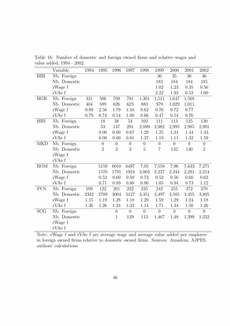
Table 16: Number of domestic and foreign owned firms and relative wages andvalue added, 1994 - 2002.

Variable 1994 1995 1996 1997 1998 1999 2000 2001 2002BIH Nb. Foreign 36 35 36 36

Nb. Domestic 183 184 184 185rWage f 1.02 1.23 0.35 0.56rVAe f 2.22 1.93 0.53 1.00

BGR Nb. Foreign 321 506 709 781 1,301 1,511 1,647 1,568Nb. Domestic 404 589 626 623 883 979 1,029 1,011rWage f 0.89 2.56 1.79 1.10 0.62 0.76 0.72 0.77rVAe f 0.79 0.74 0.54 1.06 0.66 0.47 0.54 0.76

HRV Nb. Foreign 18 38 54 102 111 113 125 130Nb. Domestic 53 147 291 2,899 2,982 2,995 2,985 2,991rWage f 0.00 0.00 0.67 1.29 1.25 1.24 1.44 1.43rVAe f 0.00 0.00 0.81 1.37 1.19 1.11 1.32 1.59

MKD Nb. Foreign 0 0 0 0 0 0 0 0Nb. Domestic 2 2 3 5 7 132 130 2rWage frVAe f

ROM Nb. Foreign 5159 6010 6497 7,05 7,558 7,96 7,633 7,271Nb. Domestic 1570 1791 1924 2,063 2,237 2,344 2,281 2,214rWage f 0.52 0.60 0.50 0.73 0.52 0.56 0.60 0.62rVAe f 0.71 0.89 0.80 0.90 1.05 0.94 0.73 1.12

SVN Nb. Foreign 109 122 201 222 235 242 255 272 270Nb. Domestic 2342 2789 3004 3127 3,351 3,497 3,585 3,455 3,805rWage f 1.15 1.19 1.28 1.18 1.20 1.59 1.29 1.24 1.18rVAe f 1.36 1.26 1.24 1.32 1.14 1.71 1.34 1.50 1.26

SCG Nb. Foreign 0 0 0 0 0 0 0Nb. Domestic 1 129 113 1,467 1,48 1,399 1,332rWage frVAe f

Note: rWage f and rVAe f are average wage and average value added per employeein foreign owned firms relative to domestic owned firms. Sources: Amadeus, AJPES,authors’ calculations.

46

1989; Grossman and Helpman, 1991; Feenstra, Markusen and Zeile, 1992) as well

as through learning by exporting into industrial countries (Clerides, Lach and Ty-

bout, 1998). In both cases it is extremely important the geographic destination of

trade flows. Firms exporting to more advanced markets can learn more through

exports due to higher quality, technical, safety and other standards they have to

meet as well as due to tougher competition (and lower markups) they are faced

with in the advanced markets. Similarly, firms importing capital and intermediate

inputs from more advanced markets have to meet according technical standards in

order to be able to use the advanced western technology. Hence, higher propensity

to trade with more advanced countries should obviously result in higher level of

productivity and faster TFP growth. Tables 17 and 18 demonstrate high depen-

dence of SEE countries on exports to and imports from advanced markets. Shares

of exports of individual SEE countries to EU-15 markets range between 65% and

75%, while share of imports from the EU-15 region is close to 80%.

On the other side, for firms operating in the area of Southeast Europe it is

crucial to have free access to as much as possible large foreign markets to place

their goods. Trade liberalization among the group of SEE countries may thus

be important for local firms to expand their sales. Tables 17 and 18 show that

countries of former Yugoslavia do continue to trade extensively with each other

with the export shares close to 15% and import shares about 10%. Bosnia (export

share to SEE region of 30%) and Macedonia (import share from SEE region of

20%) seem to rely even more heavily on SEE markets. Though beneficial for

expanding firms’ sales, it is, however, a relevant question whether high propensity

to trade within the SEE region can bring about accordingly high learning effects as

compared to the trade with advanced countries. Next section has the ambition to

empirically verify whether high propensity to export and high import penetration

from the SEE markets relative to advanced markets are about to generate similar

learning effects for individual firms.

47

Table 17: Regional export shares, 1994 - 2002, in %.

Variables 1995 1996 1997 1998 1999 2000 2001 2002BIH sh YUG 30.6 26.4 34.0 33.9

sh EU15 45.8 54.6 53.7 52.8sh EU10 8.9 13.0 9.6 8.6sh OECDoth 14.8 6.0 2.7 4.7

BGR sh YUG 0.9 6.0 4.1 3.5 4.4 4.1 3.7 1.2sh EU15 75.8 71.5 73.2 74.6 70.1 67.6 67.3 70.2sh EU10 7.9 7.8 7.2 6.8 8.7 8.9 8.5 6.4sh OECDoth 15.4 14.7 15.5 15.1 16.8 19.3 20.4 22.1

HRV sh YUG 17.4 17.1 16.4 17.3 17.5 16.2 15.3 14.4sh EU15 54.3 57.5 57.4 57.9 57.7 58.6 61.3 59.4sh EU10 24.1 21.5 20.7 19.9 19.2 17.6 17.3 19.1sh OECDoth 4.2 3.9 5.5 4.9 5.7 7.6 6.1 7.1

MKD sh YUG 8.5 15.6 19.0 11.2 14.9 14.8 5.8 3.6sh EU15 80.5 77.1 58.5 67.2 61.0 55.0 69.7 57.4sh EU10 5.9 5.6 17.8 9.7 10.6 11.6 9.1 5.7sh OECDoth 5.1 1.7 4.7 11.8 13.5 18.6 15.5 33.3

ROM sh YUG 1.0 3.7 1.9 2.3 0.9 0.9 0.9 0.6sh EU15 71.0 70.0 66.2 66.3 67.7 70.9 75.5 75.1sh EU10 8.9 9.6 10.2 17.4 13.9 12.8 11.7 12.5sh OECDoth 19.1 16.7 21.7 14.1 17.4 15.4 11.9 11.9

SVN sh YUG 12.7 14.4 15.1 15.6 13.9 14.7 16.1 15.9sh EU15 74.1 71.0 70.2 69.3 70.1 67.7 66.9 66.2sh EU10 4.9 6.0 6.7 7.4 7.8 9.0 9.2 11.3sh OECDoth 8.3 8.7 8.0 7.7 8.2 8.6 7.8 6.6

Notes: Exports shares are shares of exports of individual country to differentregions in total country’s exports calculated as averages from NACE 4-digitindustries. sh YUG is share of exports to countries of former Yugoslavia (SVN,HRV, BIH, SCG, MKD), sh EU15 is export share to old EU member states,sh EU10 is export share to new EU member states and sh OECDoth is shareof exports to other OECD countries. Source: CEPII, authors’ calculations.

48

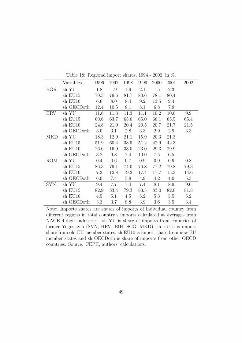
Table 18: Regional import shares, 1994 - 2002, in %.

Variables 1996 1997 1998 1999 2000 2001 2002

BGR sh YU 1.8 1.9 1.9 2.1 1.5 2.3sh EU15 79.3 79.6 81.7 80.6 78.1 80.4sh EU10 6.6 8.0 8.4 9.2 13.5 9.4sh OECDoth 12.4 10.5 8.1 8.1 6.8 7.9

HRV sh YU 11.6 11.3 11.3 11.1 10.2 10.0 9.9sh EU15 60.6 63.7 65.6 65.0 66.1 65.5 65.4sh EU10 24.8 21.9 20.4 20.5 20.7 21.7 21.5sh OECDoth 3.0 3.1 2.8 3.3 2.9 2.9 3.3

MKD sh YU 18.3 12.9 21.1 15.9 20.3 21.3sh EU15 51.9 60.4 38.5 51.2 42.9 42.3sh EU10 26.6 16.9 33.0 23.0 29.3 29.9sh OECDoth 3.2 9.8 7.4 10.0 7.5 6.5

ROM sh YU 0.4 0.6 0.7 0.9 0.9 0.9 0.8sh EU15 86.3 79.1 74.0 76.8 77.2 79.8 79.3sh EU10 7.3 12.8 19.3 17.4 17.7 15.3 14.6sh OECDoth 6.0 7.4 5.9 4.9 4.2 4.0 5.3

SVN sh YU 9.4 7.7 7.4 7.4 8.1 8.9 9.6sh EU15 82.9 83.4 79.3 83.5 83.0 82.0 81.8sh EU10 4.5 5.1 4.5 5.2 5.3 5.5 5.2sh OECDoth 3.3 3.7 8.8 3.9 3.6 3.5 3.4

Note: Imports shares are shares of imports of individual country fromdifferent regions in total country’s imports calculated as averages fromNACE 4-digit industries. sh YU is share of imports from countries offormer Yugoslavia (SVN, HRV, BIH, SCG, MKD), sh EU15 is importshare from old EU member states, sh EU10 is import share from new EUmember states and sh OECDoth is share of imports from other OECDcountries. Source: CEPII, authors’ calculations.

49

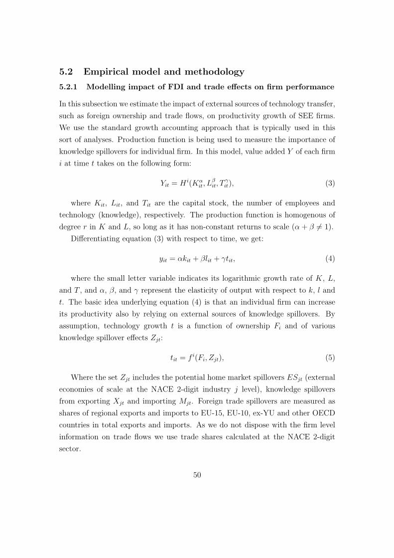
5.2 Empirical model and methodology

5.2.1 Modelling impact of FDI and trade effects on firm performance

In this subsection we estimate the impact of external sources of technology transfer,

such as foreign ownership and trade flows, on productivity growth of SEE firms.

We use the standard growth accounting approach that is typically used in this

sort of analyses. Production function is being used to measure the importance of

knowledge spillovers for individual firm. In this model, value added Y of each firm

i at time t takes on the following form:

Yit = H i(Kαit, L

βit, T

γit), (3)

where Kit, Lit, and Tit are the capital stock, the number of employees and

technology (knowledge), respectively. The production function is homogenous of

degree r in K and L, so long as it has non-constant returns to scale (α + β 6= 1).

Differentiating equation (3) with respect to time, we get:

yit = αkit + βlit + γtit, (4)

where the small letter variable indicates its logarithmic growth rate of K, L,

and T , and α, β, and γ represent the elasticity of output with respect to k, l and

t. The basic idea underlying equation (4) is that an individual firm can increase

its productivity also by relying on external sources of knowledge spillovers. By

assumption, technology growth t is a function of ownership Fi and of various

knowledge spillover effects Zjt:

tit = f i(Fi, Zjt), (5)

Where the set Zjt includes the potential home market spillovers ESjt (external

economies of scale at the NACE 2-digit industry j level), knowledge spillovers

from exporting Xjt and importing Mjt. Foreign trade spillovers are measured as

shares of regional exports and imports to EU-15, EU-10, ex-YU and other OECD

countries in total exports and imports. As we do not dispose with the firm level

information on trade flows we use trade shares calculated at the NACE 2-digit

sector.

50

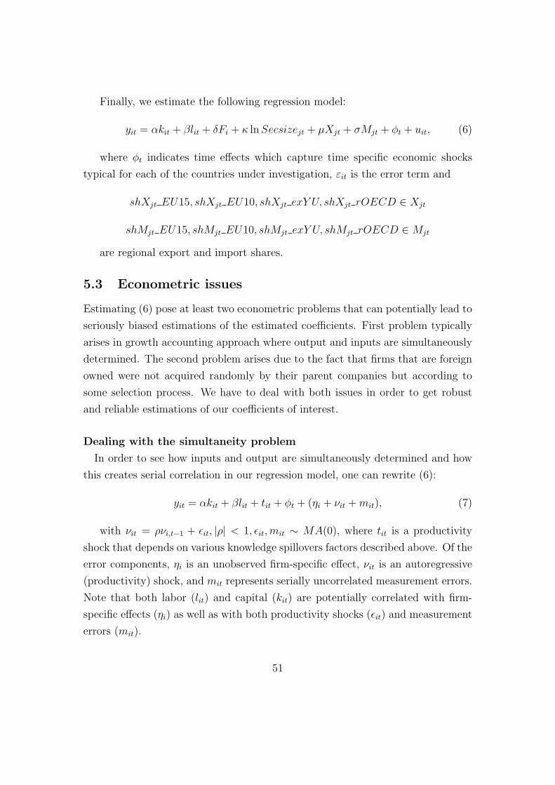
Finally, we estimate the following regression model:

yit = αkit + βlit + δFi + κ ln Secsizejt + µXjt + σMjt + φt + uit, (6)

where φt indicates time effects which capture time specific economic shocks

typical for each of the countries under investigation, εit is the error term and

shXjt EU15, shXjt EU10, shXjt exY U, shXjt rOECD ∈ Xjt

shMjt EU15, shMjt EU10, shMjt exY U, shMjt rOECD ∈ Mjt

are regional export and import shares.

5.3 Econometric issues

Estimating (6) pose at least two econometric problems that can potentially lead to

seriously biased estimations of the estimated coefficients. First problem typically

arises in growth accounting approach where output and inputs are simultaneously

determined. The second problem arises due to the fact that firms that are foreign

owned were not acquired randomly by their parent companies but according to

some selection process. We have to deal with both issues in order to get robust

and reliable estimations of our coefficients of interest.

Dealing with the simultaneity problem

In order to see how inputs and output are simultaneously determined and how

this creates serial correlation in our regression model, one can rewrite (6):

yit = αkit + βlit + tit + φt + (ηi + νit + mit), (7)

with νit = ρνi,t−1 + εit, |ρ| < 1, εit,mit ∼ MA(0), where tit is a productivity

shock that depends on various knowledge spillovers factors described above. Of the

error components, ηi is an unobserved firm-specific effect, νit is an autoregressive

(productivity) shock, and mit represents serially uncorrelated measurement errors.

Note that both labor (lit) and capital (kit) are potentially correlated with firm-

specific effects (ηi) as well as with both productivity shocks (εit) and measurement

errors (mit).

51

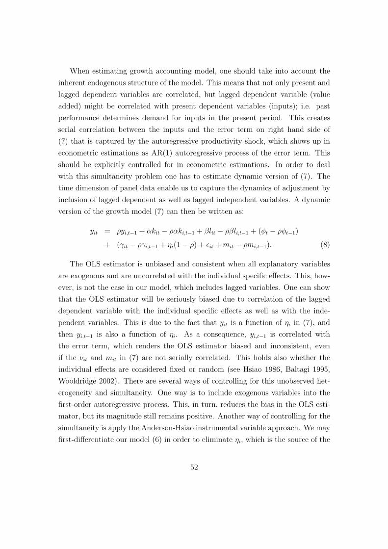
When estimating growth accounting model, one should take into account the

inherent endogenous structure of the model. This means that not only present and

lagged dependent variables are correlated, but lagged dependent variable (value

added) might be correlated with present dependent variables (inputs); i.e. past

performance determines demand for inputs in the present period. This creates

serial correlation between the inputs and the error term on right hand side of

(7) that is captured by the autoregressive productivity shock, which shows up in

econometric estimations as AR(1) autoregressive process of the error term. This

should be explicitly controlled for in econometric estimations. In order to deal

with this simultaneity problem one has to estimate dynamic version of (7). The

time dimension of panel data enable us to capture the dynamics of adjustment by

inclusion of lagged dependent as well as lagged independent variables. A dynamic

version of the growth model (7) can then be written as:

yit = ρyi,t−1 + αkit − ραki,t−1 + βlit − ρβli,t−1 + (φt − ρφt−1)

+ (γit − ργi,t−1 + ηi(1− ρ) + εit + mit − ρmi,t−1). (8)

The OLS estimator is unbiased and consistent when all explanatory variables

are exogenous and are uncorrelated with the individual specific effects. This, how-

ever, is not the case in our model, which includes lagged variables. One can show

that the OLS estimator will be seriously biased due to correlation of the lagged

dependent variable with the individual specific effects as well as with the inde-

pendent variables. This is due to the fact that yit is a function of ηi in (7), and

then yi,t−1 is also a function of ηi. As a consequence, yi,t−1 is correlated with

the error term, which renders the OLS estimator biased and inconsistent, even

if the νit and mit in (7) are not serially correlated. This holds also whether the

individual effects are considered fixed or random (see Hsiao 1986, Baltagi 1995,

Wooldridge 2002). There are several ways of controlling for this unobserved het-

erogeneity and simultaneity. One way is to include exogenous variables into the

first-order autoregressive process. This, in turn, reduces the bias in the OLS esti-

mator, but its magnitude still remains positive. Another way of controlling for the

simultaneity is apply the Anderson-Hsiao instrumental variable approach. We may

first-differentiate our model (6) in order to eliminate ηi, which is the source of the

52

bias in the OLS estimator. Then we may take the second lag of the level (yi,t−2) and

the first difference of this second lag (∆yi,t−2) as possible instruments for (∆yi,t−1),

since both are correlated with it (∆yi,t−1 = yi,t−1 − yi,t−2 ) but uncorrelated with

the error term (∆uit = uit − ui,t−1 ). This approach, though consistent, is not

efficient since it does not take into account all the available moment conditions

(i.e. restrictions on the covariances between regressors and the error term).

Hence, a natural choice of approach that allows for controlling for the unob-

served heterogeneity and simultaneity in (8) is the application of GMM (general

method of moments) estimators. As shown by Arellano and Bond (1991, 1998),

Arellano and Bover (1995) and Blundell and Bond (1998, 1999), an application

of the system GMM estimators is a more appropriate approach to dynamic panel

data than using difference GMM estimators. Our model will be estimated in first

differences in order to obtain estimates of coefficients on growth performance of

privatized companies as well as to eliminate unobserved firm-specific effects. Since

lagged level instruments used in diff-GMM approach are shown to be weak instru-

ments for first-differenced equation, we apply sys-GMM approach, which in addi-

tion to lagged levels uses also lagged first-differences as instruments for equations

in levels. As model is estimated in first differences, corresponding instruments for

(∆xi3) are (xi1) and (∆xi1) (where x stands generally for all included variables),

and so on for higher time periods. This allows for a larger set of lagged levels

and first-differences instruments and therefore to exploit fully all of the available

moment conditions. Hence, the system GMM approach maximizes both the con-

sistency as well as the efficiency of the applied estimator.

There are also other ways of dealing with simultaneity problem, such as Levin-

sohn - Petrin (1996) and Olley-Pakes (2002) approach. Both of them as well as

the system GMM approach might be used efficiently to deal with this problem.

A drawback, however, of all of these approaches is that they are computationally

very expensive and require good quality and long time series of data on inputs and

output. In our case, we are dealing with less advanced transition countries where

both the quality of datasets as well as availability of long time series is not war-

ranted. We will therefore have to limit our econometric efforts to the availability

of data.

53

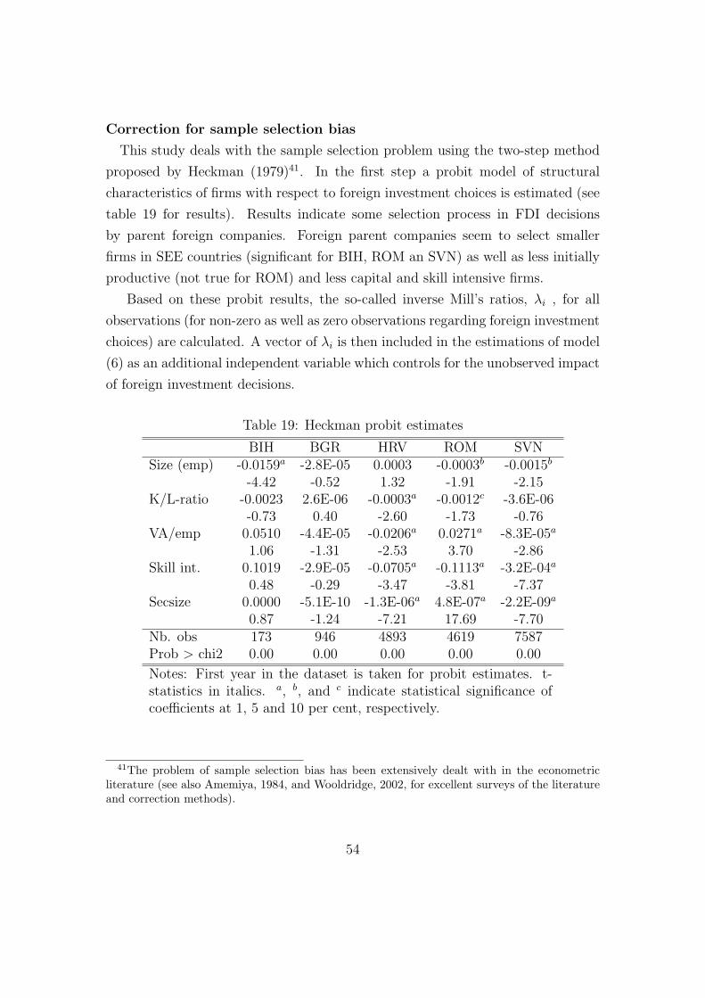
Correction for sample selection bias

This study deals with the sample selection problem using the two-step method

proposed by Heckman (1979)41. In the first step a probit model of structural

characteristics of firms with respect to foreign investment choices is estimated (see

table 19 for results). Results indicate some selection process in FDI decisions

by parent foreign companies. Foreign parent companies seem to select smaller

firms in SEE countries (significant for BIH, ROM an SVN) as well as less initially

productive (not true for ROM) and less capital and skill intensive firms.

Based on these probit results, the so-called inverse Mill’s ratios, λi , for all

observations (for non-zero as well as zero observations regarding foreign investment

choices) are calculated. A vector of λi is then included in the estimations of model

(6) as an additional independent variable which controls for the unobserved impact

of foreign investment decisions.

Table 19: Heckman probit estimates

BIH BGR HRV ROM SVNSize (emp) -0.0159a -2.8E-05 0.0003 -0.0003b -0.0015b

-4.42 -0.52 1.32 -1.91 -2.15K/L-ratio -0.0023 2.6E-06 -0.0003a -0.0012c -3.6E-06

-0.73 0.40 -2.60 -1.73 -0.76VA/emp 0.0510 -4.4E-05 -0.0206a 0.0271a -8.3E-05a

1.06 -1.31 -2.53 3.70 -2.86Skill int. 0.1019 -2.9E-05 -0.0705a -0.1113a -3.2E-04a

0.48 -0.29 -3.47 -3.81 -7.37Secsize 0.0000 -5.1E-10 -1.3E-06a 4.8E-07a -2.2E-09a

0.87 -1.24 -7.21 17.69 -7.70Nb. obs 173 946 4893 4619 7587Prob > chi2 0.00 0.00 0.00 0.00 0.00

Notes: First year in the dataset is taken for probit estimates. t-statistics in italics. a, b, and c indicate statistical significance ofcoefficients at 1, 5 and 10 per cent, respectively.

41The problem of sample selection bias has been extensively dealt with in the econometricliterature (see also Amemiya, 1984, and Wooldridge, 2002, for excellent surveys of the literatureand correction methods).

54

5.4 Results

In this section we provide estimates of the impact of foreign ownership and trade

liberalization on firm performance in SEE firms. As indicated above we are dealing

with less advanced transition countries where both the quality of datasets as well

as availability of long time series is not warranted. This can be seen in table 20

which reveals very poor availability of data for Bosnia and Macedonia (only three

years of observations). While for the other four countries data series are longer,

the quality of data in terms of the persistency of series is very poor. One can ob-

serve extremely large changes of value added, labor and value added per employee

in the early years of our sample, while in the second part of our sample period

the changes then become more moderate. This is due to the transition process

which is characterized by initial huge drop in economic activity and fast recovery

afterwards. This process of transition, thus, lacks the persistency which makes

GMM estimations less efficient as even lagged levels are poor instruments for the

model estimated in levels. Accordingly, we have to limit our econometric efforts to

the availability of data and will therefore first estimate our empirical model (6) in

log first differences (i.e. growth rates) in order to obtain estimates of coefficients

on firm’s TFP growth as well as to eliminate firm fixed effects (ηi) , which is the

source of the bias in the OLS estimator. This will also give us the benchmark

estimates. In addition, we will run GMM estimates for those countries only where

the length of the time series makes this approach reasonable.

5.4.1 Results with first differences estimation

Availability of data for imports is smaller than for exports. We therefore first

present results for the model with exports shares only and then proceed with

presenting results for the model with imports shares. As we are regressing growth

rates of inputs on the growth rate of value added, one can interpret the results in

terms of the contribution of different factors to the growth of TFP.

Results presented in table 21 confirm for three countries (Bosnia, Croatia and

Slovenia) faster TFP growth in foreign owned firms as compared to purely domestic

owned firms. In Romania, in contrast we find faster TFP growth in domestic owned

firms, while in Bulgaria no significant differences have been found. The results are

55

Table 20: Average rates of growth of value added, labor and value added peremployee in SEE, 1994-2002, in %.

1994 1995 1996 1997 1998 1999 2000 2001 2002BIH dVA -45.5 120.4 6.8

dL 4.1 -32.3 -2.3dVAe -49.7 153.9 9.5dVAe f -8.2 17.2 5.2

BGR dVA -74.8 -516.7 -108.7 65.7 34.4 -5.2 6.2 7.9 4.9dL -7.1 0.6 0.9 1.7 0.4 -3.2 -4.0 -6.2 5.8dVAe -23.9 -592.1 -108.3 67.9 37.1 -8.0 14.7 5.8 -0.1dVAe f -9.6 -234.4 -48.2 30.4 16.3 -3.1 7.6 3.9 -0.2

HRV dVA 6.9 -0.5 -7.1 7.4 11.0 12.7 1.0dL -1.4 -3.5 -2.5 5.7 3.1 5.2 4.6dVAe 5.6 12.4 -5.6 0.4 7.7 7.0 -4.3dVAe f 6.4 16.5 -1.0 0.4 0.5 0.1 0.3

MKD dVA -7.4dL -1.3 -2.6 -14.8dVAe -4.6dVAe f

ROM dVA 10.1 1.3 -4.4 -0.8 8.2 25.0 -3.5dL 6.4 19.4 15.4 8.6 11.5 2.7 -5.7dVAe 7.0 -13.8 -13.8 -4.4 0.9 18.0 -4.5dVAe f 5.8 -11.9 -10.3 -5.0 -0.7 13.4 -4.0

SVN dVA 25.2 22.6 21.2 11.6 14.2 10.7 12.2 9.9dL 7.6 3.7 5.1 4.4 3.9 4.0 3.5 0.6dVAe 17.6 19.0 16.1 7.2 10.3 6.6 8.8 9.3dVAe f -0.4 17.9 3.7 1.0 1.4 3.1 5.8 -1.4

Sources: Amadeus, AJPES, authors’ calculations.

56

Table 21: Impact of FDI and export propensity on productivity growth in SEEfirms, period 1995 - 2002 (first differences specification).

BIH BGR HRV ROM SVN MKDdK 0.137 0.796a 0.067a 0.539a 0.339a 0.357c

0.56 48.61 12.32 68.96 34.11 1.98dL 0.067 0.294a 0.424a 0.319a 0.540a 0.080

0.47 11.82 44.12 45.26 44.59 0.29Foreign 0.441a 0.016 0.066b -0.064a 0.048a

4.40 0.79 2.16 -7.32 2.49log Secsize 0.008 -0.001 -0.126a -0.079a -0.057a 0.038

0.18 -0.10 -18.63 -8.90 -7.71 1.22EXsh EU15 -0.611 0.062 0.036 0.248a 0.146c 0.489

-0.85 0.77 0.25 4.78 1.72 0.38EXsh OECDoth -0.197 -0.040 0.014 0.304a *0.212 0.705

-0.27 -0.35 0.08 5.94 1.93 0.52EXsh YU -0.467 -0.391 0.115 0.703a 0.006 -0.756

-0.54 -1.38 0.40 2.87 0.06 -0.25lambda 0.017 -0.466 -1.662a 0.185a -1.167a

0.25 -0.98 -28.43 10.37 -20.70Year dummies Yes Yes Yes Yes Yes YesNb. Obs 181 4461 21368 33366 23464 106Adj R2 0.135 0.807 0.113 0.248 0.186 0.149Prob > chi2 0.00 0.00 0.00 0.00 0.00Nb. BS Replications 500

Notes: Dependent variable dVA (value added, specified in log first differ-ences). t-statistics in italics. a, b, and c indicate statistical significance ofcoefficients at 1, 5 and 10 per cent, respectively.

57

in line with the results on the selection process which showed that foreign parent

companies have acquired mainly least productive, less capital and skill intensive

firms. However, one can expect that after restructuring these firms would improve

their TFP at a much faster rate than purely domestic owned firms.

In terms of the impact of export propensity to different regional markets we

find that in Romania and Slovenia higher propensity to export to advanced mar-

kets (EU-15, rest of OECD countries) has a larger impact on TFP growth than

exporting to less advanced markets such as new EU member states and countries of

former Yugoslavia. In other words, exporting to advanced countries provide much

larger learning effects for a typical firm than exporting to less advanced markets.

Including the imports shares into our empirical model does not alter our results

on export shares (see table 22). The role of imports follows a similar path as

exporting. Importing from the advanced EU and OECD countries is important

for firms in Romania. At the same time, for firms in Romania and Macedonia

importing from countries of former Yugoslavia provides a dominating learning

effect. For other countries in our sample no learning effects from exporting to and

importing from individual geographic regions could be found. However, in none

of the countries significant negative effects of trade shares on firm’s performance

is found. Thus, in terms of policy implications, only in some of the countries

liberalization of bilateral trade within the SEE region might be an important engine

of firms’ growth.

5.4.2 Results with system GMM estimation

In order to control for simultaneity between the inputs and output we estimate

a dynamic model by employing the system GMM estimations for four countries

with longer time series. Results in table 23 basically confirm results obtained by

first differences estimations. In particular, foreign ownership remains significant

determinant of TFP growth in Croatia and Slovenia.

Unfortunately, positive impact of high export propensity to EU-15 and other

OECD countries is not being preserved for Croatia, Slovenia and Romania, while

in Romania a positive impact of high imports from the EU-15 and other OECD

countries is still preserved. These differences in estimated coefficients between the

first differences estimator and GMM estimator might arise due to poor quality

58

Table 22: Impact of FDI, export and import propensity on productivity growth inSEE firms, period 1995 - 2002.

BGR HRV ROM SVN MKDdK 0.464a 0.086a 0.533a 0.365a 0.374c

15.46 8.71 57.65 27.49 1.67dL 0.340a 0.458a 0.319a 0.525a 0.045

11.75 27.35 38.36 33.39 0.14Foreign 0.021 0.037 -0.087a 0.035

0.84 1.15 -8.24 1.46log Secsize -0.013 -0.074a -0.137a -0.080a -0.027

-0.83 -5.97 -10.10 -8.35 -0.45EXsh EU15 0.156 0.370c 0.056 *0.173 0.665

1.57 1.75 0.88 1.70 0.42EXsh OECDoth 0.056 0.315 0.238a 0.390a 0.471

0.40 1.21 3.71 2.83 0.27EXsh YU -0.330 0.620 0.192 0.111 -1.194

-0.87 1.50 0.70 0.89 -0.33IMsh EU15 -0.115 -0.219 0.651a 0.251 1.895

-0.56 -1.14 8.51 1.31 1.52IMsh OECDoth -0.110 -0.276 1.329a 0.177 0.649

-0.44 -0.91 8.29 0.92 0.18IMsh YU 0.086 -0.606 1.647a -0.144 5.990c

0.14 -1.08 3.28 -0.75 1.66λ 0.779 -1.123a 0.384a -1.548a

1.00 -10.70 13.49 -19.42Year dummies Yes Yes Yes Yes YesNb. Obs 3193 6860 24899 14349 92Overall R2 0.317 0.134 0.244 0.186 0.202Prob > chi2 0.00 0.00 0.00 0.00Nb. BS Replications 500

Notes: Dependent variable dVA (value added, specified in logfirst differences). t-statistics in italics. a and c indicate statisticalsignificance of coefficients at 1, 5 and 10 per cent, respectively.

59

Table 23: Impact of FDI, export and import propensity on productivity growth inSEE firms, period 1995 - 2002, system GMM estimations.

BGR SVN HRV ROMdVA 1 0.138c 0.138b 0.303a 0.220a

1.92 2.29 4.73 5.12dK 0.562a 0.302a 0.047c 0.506a

5.43 5.05 1.90 12.16dL 0.359a 0.317a 0.634a 0.413a

3.14 3.67 8.87 8.77Foreign 0.225 0.028a 0.011c 0.061

0.76 5.23 1.84 0.51log Secsize -0.053 -0.229c -0.146 -1.216a

-0.47 -1.92 -0.75 -4.79EXsh EU15 0.825 0.163 -1.225 -0.721b

0.93 0.50 -1.08 -2.15EXsh OECDoth -0.280 0.644 -1.907 0.136

-0.41 1.14 -0.85 0.77EXsh YU 4.535 0.179 2.82 1.676a

1.09 0.35 -1.17 4.50IMsh EU15 -0.539 -2.717 0.550 3.142a

-0.56 -0.96 0.30 5.15IMsh OECDoth -0.198 -2.921 0.495 5.461a

-0.19 -1.01 0.18 6.02IMsh YU -3.203 -3.743 1.110 -2.597

-0.84 -1.12 0.20 -0.30lambda -7.926 -4.417a -5.185a 2.655a

-0.89 -6.11 -2.70 8.07Year dummies Yes Yes Yes YesNb. Obs 3568 14352 6916 25418Prob > chi2 0.000 0.000 0.000 0.000Hansen test of overid. (p) 0.29 0.001 0.961 0AR(1) test (p) -3.49 -6.4 -7.6 -9.54AR(2) test (p) -1.35 0.45 0.91 0.76

Notes: Dependent variable dVA (value added, specified in logfirst differences). t-statistics in italics. a, b, and c indicatestatistical significance of coefficients at 1, 5 and 10 per cent,respectively.

60

of the data and due to the lack of the persistency of datasets. Therefore, GMM

estimations are likely to be less efficient due to the fact that even lagged levels are

poor instruments for the model estimated in levels.

6 Concluding remarks

In this study, we first estimate, on aggregated and sectoral data, the degree of

trade intensity of SEE countries. Then we evaluate their trade potentials in the

context of trade liberalization between themselves and with the EU. Second, we

estimate the impact of tariff and nontariff barriers on manufactured exports. To

these ends, we use a gravity equation. Finally, we investigate the impact of trade

liberalization on performance of firms.

We find that determinants of trade volumes and the explanatory power of

the gravity equation differ according to the sector. Trade in sectors intensive in

natural resources is less explained by the gravity equation. Moreover, our sectoral

study shows that trade volumes in some sectors are lower than their potential.

Examples are trade of wood and textile products between SEE countries and trade

of agricultural products between SEE countries and the EU.

One can also draw some interesting conclusions about the potential effects of

preferential trade agreements signed by the SEE countries between themselves and

with the EU. First, trade potentials of SEE countries with the EU are reached in

almost all the sectors. However, this average result hides a huge difference between

Eastern Balkans and Western Balkans. The former have outreached their potential

and the latter have not. One can therefore expect that trade preferences granted

by the EU to Western Balkans, at the beginning of the years 2000, will enhance

trade. On the other hand trade flows between SEE countries and between them

and CEE countries have outreached their potential for almost all sectors. However,

the experiences of Bulgaria and Romania showed that one can expect limited gains

from East-East type preferential trade agreements, even for manufactured goods.

Finally, an important result is the very low integration of these countries to the

world economy. This result confirm the necessity for SEE countries to continue

trade openness.

We find significant effects of policy measures on manufactured exports of Balkan

61

countries. Results display however significant differences between TBs and NTBs

estimates on trade. The latter exhibit larger effects on trade. Since NTBs are

increasing, probably to replace the decrease of TBs, this result is worrying. A one

point increase of NTBs sharply decreases exports.

However, one has to be cautious interpreting results since the tariff and nontariff

barriers variables are quite crude measures of protection. Furthermore, the trend of

each variable is computed with incomplete information concerning some products

and years. Nonetheless, results are quite intuitive. The difference between both

estimates is robust to different specifications and maybe explained by the domestic

firms behavior. They may push to replace TBs by NTBs. In this case, protection is

endogenous not exogenous. In response to increased import penetration, Balkans’

partners intensify their lobbying activity for greater protection. Trefler (1993) finds

that when trade protection is modeled endogenously, its restrictive impact on trade

is large, 10 times the size obtained from treating protection exogenously. However,

implementing such an estimation strategy is data demanding, since we should

estimate simultaneously both exports and TBs (or NTBs) equations. Concerning

other data requirements, results may be improved if we control for additional sector

characteristics, such as size of firms or capital stocks.

Finally, we investigate effects of trade liberalization on firm performance. We do

not find a general pattern of uniformly significant impact of extensive trade flows

on individual firm’s TFP growth. Specifically, only in Romania and Slovenia,

higher propensity to export to advanced markets has a larger impact on TFP

growth than exporting to less advanced markets such as new EU members and

countries of former Yugoslavia. In other words, in these two countries exporting

to advanced countries provide much larger learning effects for a typical firm than

exporting to less advanced markets. The role of imports follows a similar path

as exporting. Importing from the advanced countries is important for firms in

Romania. At the same time, for firms in Romania and Macedonia importing

from countries of former Yugoslavia provides a dominating learning effect. For

other countries in our sample no learning effects from exporting to and importing

from individual geographic regions could be found. Thus, one cannot imply that

liberalization of bilateral trade within the region of SEE or with the other regions

will have uniformly significant impact on individual firm’s performance, but in

62

some of the countries analysed trade liberalization might be an important engine

of firms’ productivity growth.

Our results also indicate some selection process in FDI decisions by parent

foreign companies. Foreign parent companies seem to select smaller firms in SEE

as well as least productive, less capital and skill intensive firms. However, we find

contrasting results on the impact on foreign ownership on TFP growth. Three

countries (Bosnia, Croatia and Slovenia) experience faster TFP growth in foreign

owned firms. In Romania, in contrast we find faster TFP growth in domestic owned

firms, while in Bulgaria no significant differences have been found. However, one

can expect that after restructuring these firms would improve their TFP at a much

faster rate than purely domestic owned firms.

Of course, one has again to be cautious interpreting results. Although we make

use of the best available data, in most of the SEE countries we face a problem

of lacking persistency of datasets, which prevents from getting very clear and

conclusive results. We therefore make a request for better information collection

and for its ready provision to researchers.

63

References

Abraham F. and Van Hove J. (2005), “The rise of China: prospects of regional

trade policy”, Review of World Economics, 141(3).

Adam A., Kosma T.S. and McHugh J. (2003), “Trade- liberalisation strategies,

what could South-Eastern Europe learn from CEFTA and BEFTA?”, IMF Work-

ing Paper, 03/239, Washington.

Amemiya T. (1984), “Tobit models. A Survey”, Journal of Econometrics, 24: 3-61.

Anderson J.E. and Van Wincoop E. (2003), “Gravity with gravitas: a solution to

the border effect puzzle”, American Economic Review, 93(1), 170-192.

Anderson J.E. and Van Wincoop E. (2004), “Trade cost”, Journal of Economic

Literature, 42, 691-751.

Andreff M., Andreff W. and Boudier-Bensebaa F. (2001), “Sous-traitance

internationale de faconnage et trafic de perfectionnement passif entre les pays de

l’Union europeenne et de l’Europe de l’Est”, Revue d’Etudes Comparatives Est-

Ouest, 32(2), 5-34.

Arellano M. and S.R. Bond (1991), “Some Tests of Specification for Panel Data:

Monte Carlo Evidence and an Application to Employment Equations”, Review of

Economic Studies, 58: 277-297.

Arellano, M. and O. Bover. (1995), “Another Look at the Instrumental-variable

Estimation of Error-components Model”, Journal of Econometrics, 68: 29-52.

Arellano, M. and S.R. Bond. (1998), “Dynamic Panel Data Estimation using

DPD98 for GAUSS”, Mimeo, Institute for Fiscal Studies, London.

Arnon A., Spivak A. and Weinblatt J. (1996), “Potential for trade between Israel,

the Palestinians and Jordan”, World Economy, 19, 113-14.

Babetskaia-Kukharchuk O. and Maurel M. (2004), “Russia’s accession to the

WTO: the potential for trade increase”, Journal of Comparative Economics, 32,

680-99.

64

Baier S.L. and Bergstrand J. (2003), “Endogeneous free-trade agreements and the

gravity equation”, mimeo.

Baier S.L. and Bergstrand J. (2004), “Economic determinants of free-trade agree-

ments”, Journal of International Economics, 64(1), 29-63.

Baldwin R. (1993), “The potential for trade between the countries of EFTA and

Central and Eastern Europe”, CEPR Discussion Paper, 853, Center for Economic

Policy Research, London.

Baldwin R. (1994), Towards an integrated Europe, CEPR, Londres.

Baldwin R., Skudelny F. and Taglioni D. (2005), “Trade effects of the Euro:

Evidence from sectoral data”, European Central Bank Working Paper, 446.

Baltagi, H.B. (1995), Econometric Analysis of Panel Data, Chichester: John Wiley

& Sons.

Basu, S. and J. Fernald. (1995), “Aggregate Productivity and the Productivity of

Aggregates”, NBER Working Paper 5382.

Batra A. (2004),“India’s global trade potential: the gravity model approach”, ICRIER

Working Paper, 151, Indian Council for Research on International Economic Re-

lations, New Delhi.

Bergstrand J.H. (1989), “The generalized gravity equation, monopolistic competi-

tion, and the factor-proportions theory in international trade”, Review of Eco-

nomics and Statistics, 71(1), 143-53.

Bjelic P. (2005), “Trade policy of the EU as a factor of regional trade integration in

South-Eastern Europe”, Discussion Paper - Center for the Study of Global Gov-

ernance, 36, London School of Economics.

Blundell, R.W. and S.R. Bond. (1998), “Initial Conditions and Moment Restric-

tions in Dynamic Panel Data Models”, Journal of Econometrics, 87: 115-143.

Blundell, R.W. and S.R. Bond. (1999), “GMM Estimation with Persistent Panel

Data: An Application to Production Functions”, Institute for Fiscal Studies, Lon-

don, WP No. W99/4.

65

Boillot J.-J, Lefilleur J. and Lepape Y. (2003), “Quel avenir au commerce intra-

CEEC ? Une analyse actuelle et previsionnelle des echanges en Europe centrale et

orientale”, mimeo, DREE-MINEFI, Paris.

Borensztein, E., J. De Gregorio, and J.W. Lee. (1998), “How Does Foreign

Direct Investment Affect Economic Growth?”, Journal of International Economics,

45: 115-135.

Brenton P. and Di Mauro F. (1998), “Is there any potential in trade in sensitive

industrial products between the CEECs and the EU?”, World Economy, 21(3),

285-304.

Brulhart M. and Kelly M.J. (1999), “Ireland’s trading potential with Central and

Eastern European countries: a gravity study”, The Economic and Social Review,

30(2), 159-74.

Buch C. and Piazolo D. (2001), “Capital and trade flows in Europe and the impact

of enlargement”, Economic Systems, 25(3), 183-214.

Bussiere M., Fidrmuc J. and Schnatz B. (2004), “Trade integration of the new EU

member and selected South Eastern European countries: Lessons from a gravity

model”, Oesterreichische Nationalbank Conference on European Economic Inte-

gration, 28-30 novembre.

Caetano J. and Galego A. (2003), “An analysis of actual and potential trade

between the EU countries and the Eastern European countries”, Documento de

Trabalho, 3, University of Evora.

Christie E. (2002), “Potential trade in South-Eastern Europe: A gravity model ap-

proach”, WIIW Working Paper, 21.

Clerides, S., S. Lach, and J. Tybout (1998), “Is Learning-by-Exporting Impor-

tant? Micro-Dynamic Evidence from Colombia, Mexico and Morocco”, Quarterly

Journal of Economics, 113: 903-947.

Coe, D. and E. Helpman (1995), “International R&D Spillovers”, European Eco-

nomic Review, 39: 859-887.

66

Coe, D., E. Helpman, and A. Hoffmaister. (1997), “North-South R&D Spillovers”,

Economic Journal, 107: 134-149.

Commission of the European Communities (2003), “Le processus de stabilisation

et d’association en faveur de l’Europe du Sud-Est”, Deuxieme Rapport annuel,

COM(2003)139, Final.

Daianu D. and Veremis T. (2001), “Balkan reconstruction: introduction”, Journal

of Southeast European and Black Sea Studies, 1(1), 1-11.

Damijan, J.P., M. Knell. (2005), “How Important is Trade and Foreign Ownership

in Closing the Technology Gap: Evidence from Estonia and Slovenia”, Review of

World Economics (Weltwirtschaftliches Archiv), 141: 271-295.

Damijan, J.P., M. Knell, B. Majcen, and M. Rojec. (2003), “The Role of FDI,

R&D Accumulation and Trade in Transferring Technology to Transition Coun-

tries: Evidence from Firm Panel Data for Eight Transition Countries”, Economic

Systems, 27: 189-204.

Damijan, P.J, M. Knell, B. Majcen, M. Rojec. (2003), “Technology Transfer

through FDI in Top-10 Transition Countries: How Important are Direct Effects,

Horizontal and Vertical Spillovers?”, William Davidson Institute Working paper,

no.549.

Dangerfield M. (2001), Subregional economic cooperation in Central and Eastern

Europe: the political economy of CEFTA, Edward Elgar, Cheltenham.

Deardoff A. and Stern R. (1986) The Michigan model of world production and

trade: theory and applications, Cambridge, Mass.: MIT Press.

De Benedictis L. and Vicarelli C. (2004), “Trade potentials in gravity panel data

models”, ISAE Working Paper, 44, University of Macerata.

De Sousa J. and Lamotte O. (2005), “Does transition lead to trade disintegration

? Evidence from former Yugoslavia”, working paper, Universite de Paris I.

Dimelis S. and Gatsios K. (1994), “Trade with CEE: the case of Greece”, CEPR

Discussion Paper, 1005, Center for Economic Policy Research, London.

67

Duc C., Granger C., Lavallee E. and Siroen J.-M. (2004), “Does deep inte-

gration foster trade? Empirical evidence and simulations for the EU democratic

and anti-corruption criteria”, Cahier de recherche EURIsCO, 2004-15, Universite

de Paris Dauphine.

EBRD (European Bank of Reconstruction and Development) (2004), Tran-

sition Report, London.

Eaton, J. and S. Kortum. (1996), “Trade in Ideas: Patenting and Productivity in

the OECD”, Journal of International Economics, 40: 251-271.

Egger P. (2002), “An econometric view of the estimation of gravity models and the

calculation of trade potentials”, World Economy, 25(2), 297-312.

Ekholm K., Torstensson J. and Torstensson R. (1996), “The economics of the

Middle East peace process: Are there prospects for trade and growth?”, World

Economy, 19, 555-74.

Feenstra, R., J. Markusen, and W. Zeile. (1992), “Accounting for Growth with

New Inputs: Theory and Evidence”, American Economic Review, 82: 415-421.

Festoc F. (1997), “Le potentiel de croissance du commerce des pays d’Europe centrale

et orientale avec la France et ses principaux partenaires”, Economie et Prevision,

(128), 161-81.

Fidrmuc J. (1999), “Trade diversion in left-outs in eastward enlargement of the Euro-

pean Union: the case of Slovakia”, Europe-Asia Studies, 51(4), 633-45.

Fidrmuc J., Huber P. and Michalek J.J. (2001), “Poland’s accession to the Euro-

pean Union: demand for protection of selected sensitive products”, MOCT-MOST,

11(1), 45-67.

Fidrmuc J. (2004), “The core and the periphery of the world economy”, Journal of

International Trade and Economic Development, 13(1), 89-106.

Fontagne L., Freudenberg M. and Pajot M. (1999) “Le potentiel d’echange

entre l’Union europeenne et les CEEC : un reexamen”, Revue economique, 50(6),

1139-68.

68

Fontagne L., Pajot M. and Pasteels, J.-M. (2002), “Potentiels de commerce

entre economies heterogenes: un petit mode d’emploi des modeles de gravite”,

Economie et Prevision, 152-53(1-2), 115-40.

Fritz H. and Hoen H.W. (2000), “The European Union’s trade policy towards Cen-

tral and Eastern Europe: still a ’sensitive’ argument for joining the Union ?”,

Economic Systems, 24(1), 25-50.

Fukao K., Okubo T. and Stern R. (2003), “An econometric analysis of trade di-

version under NAFTA”, The North American Journal of Economics and Finance,

14, 3-24.

Greene, W.H. (1997), Econometric Analysis, 3rd edition, New Jersey: Prentice-Hall

International.

Greenaway D. and Milner C. (2002), “Regionalism and Gravity”, Scottich Journal

of Political Economy, 49(5), 574-585.

Griliches, Z. (1979), “Issues in Assessing the Contribution of Research and Develop-

ment to Productivity Growth”, The Bell Journal of Economics, 10: 92-116.

Griliches, Z. and J. Mairesse. (1995), “Production Functions: the Search for

Identification”, NBER Working Paper 5067.

Gros D. and Gonciarz A. (1996), “A note on the trade potential of Central and

Eastern Europe”, European Journal of Political Economy, 12(4), 709-21.

Hamilton C.B. and Winters L.A. (1992), “Opening up international trade with

Eastern Europe”, Economic Policy, 14(4), 77-116.

Hausman, A.J. (1978), “Specification Tests in Econometrics”, Econometrica, 46: 1251-

1271.

Hausman J. and Taylor W. (1981),“Panel data and unobservable individual effects”,

Econometrica, 49, 1377-98.

Havrylyshyn O. and Pritchett L. (1991), “European trade patterns after the

transitions”, World Bank Working Paper, 748.

69

Havrylyshyn O. and Al-Atrash H. (1998), “Opening up and geographic diversifi-

cation of trade in transition economies ”, IMF Working Paper, 22.

Heckman, J.J. (1979), “Sample Selection Bias as a Specification Error”, Econometrica,

47: 153-161.

Hsiao, C. (1986), Analysis of Panel Data, Cambridge, MA: Cambridge University

Press.

International Trade Center (ITC) (2003), “TradeSim, A gravity model for the

calculation of trade potentials for developing countries and economies in transi-

tion”, UNCTAD/WTO, Geneva.

Jakab Z.M., Kovacs M.A. and Oszlay A. (2001), “How far has trade integration

advanced?: An analysis of the actual and potential trade of three Central and

Eastern European countries ”, Journal of Comparative Economics, 29 (2), 276-

92.

Kaminski B. and de la Rocha M. (2003), “Stabilization and association process

in the Balkans: integration options and their assessment”, World Bank Policy

Research Working Paper, 3108.

Kovac O. (1998), “Trade flows among Balkan countries and opportunities with SECI”,

American Association for the Advancement of Slavic Studies (AAASS) Conference,

Boca Raton.

Lamotte O. (2003), “Une zone de libre-echange en Europe du Sud-Est: pertinence et

limites”, Le Courrier des Pays de l’Est, 1039, 4-17.

Lopandic D. (1999), “Multilateral cooperation in South-Eastern Europe”, 67-84, in

Minic J., South Eastern Europe 2000, A view from Serbia, Stubovi Kulture,

Belgrade.

Lopandic D. (2001), Regional initiatives in South Eastern Europe, European Move-

ment in Serbia, Belgrade.

Marques H. and Metcalf H. (2005), “What determines sectoral trade in the en-

larged EU?”, Review of Development Economics, 9(2), 197-231.

70

Martinez-Zarzoso I. and Nowak-Lehmann F. (2003), “Augmented gravity model:

An empirical application to Mercosur-European Union trade flows”, Journal of

Applied Economics, 6(2), 291-316.

Matyas L. (1997), “Proper econometric specification of the gravity model”, World

Economy, 21(3), 363-368.

Mayer T. and Zignago S. (2005), “Market Access in Global and Regional Trade”,

Cepii Working paper, 2.

Mansfield, E. and M. Romeo. (1980), “Technology Transfer to Overseas Sub-

sidiaries by U.S. Based Firms”” Quarterly Journal of Economics, 95, 737-750.

McPherson M. and Trumbull W. (2003), “What if US-Cuban trade were based on

fundamentals instead of political policy? Estimating potential trade with Cuba,

Cuba in Transition”, Papers and Proceedings of the 13th annual meeting of the

ASCE, Coral Gables, 7-9 aout.

Messerlin P.A. and Miroudot S. (2004), “Trade liberalisation in South-Eastern

Europe. Review of conformity of 23 FTA with the MoU”, GEM, Sciences Po,

Paris.

Nilsson L. (2000), “Trade integration and the EU economic membership criteria”,

European Journal of Political Economy, 16(4), 807-27.

Olley, S.G. and A. Pakes. (1996), “The Dynamics of Productivity in the Telecom-

munications Equipment Industry”, Econometrica, 64, 1263-1297.

Wooldridge, J. (2002), Econometric Analysis of Cross Section and Panel Data, Cam-

bridge, Mass.: MIT Press.

Paas T. (2002), “Gravity approach for exploring Baltic Sea regional integration in the

field of international trade”, HWWA Discussion Paper, 180.

Peridy N. (2003), “Exchange rate volatility, sectoral trade, and the aggregation bias”,

Review of World Economics, 139(3), 389-418.

71

Peridy N. (2004), “The new US trans-ocean free trade initiatives: Estimating export

and FDI potentials from dynamic panel data models”, Economic Bulletin, 6(9),

1-12.

Peridy N. (2005a), “Towards a new trade policy between the USA and Middle-East

countries: Estimating trade resistance and export potential”, World Economy,

28(4), 491-518.

Peridy N. (2005b), “Trade prospects of the new EU neighborhood policy: Evidence

from Hausman and Taylor’s models”, Global Economy Journal, 5(1).

Puga D. and Venables A.J. (1998), “Trading arrangements and industrial develop-

ment”, The World Bank Economic Review, 12(2), 221-49.

Rose A.K. (2005), “ Do we really know that the WTO increases trade?”, American

Economic Review, 94(1), 98-114.

Subramanian A. and Wei S.J. (2003), “The WTO promotes trade, strongly but

unevenly”, NBER Working Paper, 10024.

Trefler D (1993), “Trade liberalization and the theory of endogenous protection:

an econometric study of U.S. import policy, Journal of Political Economy, 101,

138-160.

Uvalic M. (2001), “Regional cooperation in Southeast Europe”, in Veremis Th. and

Daianu D., (ed.) Balkan reconstruction, Franck Cass Publishers, London, 55-75.

Van Bergeijk P.A.G. and Oldersma H. (1990), “Detente, market-oriented reform

and German unification: Potential consequences for the world trade system”, Kyk-

los, 43(4), 599-609.

Van Brabant J. (2001), “South-Eastern Europe, transitions and the EU - Is ever

widening desirable?”, MOCT-MOST, 11, 295-325.

Vittas H. and Mauro P. (1997), “Potential trade with core and periphery: industry

differences in trade patterns”, in Black S. (ed.), Europe’s economy looks East,

Cambridge University Press, Cambridge.

72

Wang Z.K. and Winters A. (1992), “The trading potential of Eastern Europe”,

Journal of Economic Integration, 7, 113-36.

Welfens P.J.J. (2001), Stabilizing and integrating the Balkans, Springer Verlag,

Berlin.

World Bank (2000), The road to stability and prosperity in South Eastern Europe: a

regional strategy paper, World Bank, Washington.

Woolridge, J (2003), Introductory econometrics, second edition, South-Western Col-

lege.

7 Appendix

Table 24: Free trade agreements between SEE countries

Albania Bosnia-H. Bulgaria Croatia Macedonia Moldova Romania Serbia-M.Albania - 12/04 09/03 06/03 07/02 11/04 01/04 08/04Bosnia-H. 12/04 12/04 01/05 07/02 05/04 12/04 06/02Bulgaria 09/03 12/04 03/03* 01/00 11/04 07/97* 06/04Croatia 06/03 01/05 03/03* 06/97 10/04 03/03* 07/04Macedonia 07/02 07/02 01/00 06/97 01/05 01/04 05/05Moldova 11/04 05/04 11/04 10/04 01/05 11/94 09/04Romania 01/04 12/04 07/97* 03/03* 01/04 11/94 - 01/07/04Serbia-M. 08/04 06/02 06/04 07/04 05/05 09/04 07/04 -Notes: Table realized from www.stabilitypact.org, as of the 9th of June 2005. Dates refer to theentry in force of the agreements (dd/mm/yy). *Indicates that trade liberalization took place in theframework of the CEFTA (Central European Free Trade Agreement). The entry in the CEFTAends de facto bilateral agreements signed with CEFTA country members.

73

Tab

le25

:R

evie

wof

the

lite

ratu

reusi

ng

sect

oral

estim

atio

ns

ofth

egr

avity

equat

ion

Ref

eren

ces

Sam

ple

Met

hod

Mai

nre

sult

s(c

ountr

y,se

ctor

s,per

iod)

Ber

gstr

and

(198

9)16

OE

CD

coun

trie

s,9

sect

ors,

1965

-66-

75-7

6O

LS

Supp

lyan

dde

man

del

astici

ties

diffe

rac

-co

rdin

gto

the

sect

or.

Vitta

san

dM

auro

(199

7)O

EC

Dco

untr

ies,

5se

nsitiv

ese

c-to

rs,1

993

OLS

Cal

cula

tion

ofth

etr

ade

pote

ntia

lof

the

CE

EC

;C

EE

C-E

Utr

ade

ofse

nsitiv

epr

od-

ucts

islo

wer

than

its

pote

ntia

l.B

rent

onan

dM

auro

(199

8)45

coun

trie

s(O

EC

D+

CE

EC

),9

sect

ors,

1995

OLS

Cal

cula

tion

ofth

etr

ade

pote

ntia

lof

the

CE

EC

;the

reis

nopo

tent

ialf

oran

incr

ease

ofC

EE

Cex

port

sto

war

dsth

eE

U.

Fid

rmuc

(199

9)O

EC

Dco

untr

ies,

7se

ctor

s,19

89O

LS

Cal

cula

tion

ofth

etr

ade

pote

ntia

lof

Slo-

vaki

a;th

ere

isa

pote

ntia

lwith

allc

ount

ries

exce

ptth

eC

zech

Rep

ublic

.Fid

rmuc

etal

ii(2

001)

22O

EC

Dco

untr

ies,

26pr

oduc

ts,

1994

OLS

Cal

cula

tion

ofth

etr

ade

pote

ntia

lof

Pol

and;

the

effec

tsof

EU

enla

rgem

ent

ontr

ade

diffe

rac

cord

ing

toth

ese

ctor

s.Fo

ntag

neet

alii

(200

2)53

expo

rter

s,75

impo

rter

s(D

C+

OE

CD

),14

sect

ors,

1995

-96

OLS

Cal

cula

tion

ofth

etr

ade

pote

ntia

lof

Tur

key;

shar

eof

text

ilein

the

expo

rts

ishi

gher

toits

pote

ntia

l.Fu

kao

etal

ii(2

003)

US

impo

rts,

70pr

oduc

ts,

1992

-98

OLS,

coun

try

and

tim

efix

edeff

ects

NA

FTA

has

dive

rted

trad

e,es

peci

ally

inth

ete

xtile

.

Subr

aman

ian

and

Wei

(200

3)Im

port

sof

172

coun

trie

s,se

n-si

tive

/non

sens

itiv

epr

oduc

ts,

1950

-200

0

OLS,

coun

try

fixed

effec

tsT

heG

AT

T/W

TO

hasa

posi

tive

impa

cton

the

impo

rts

ofin

dust

rial

ized

coun

trie

s,ex

-ce

ptin

the

sens

itiv

ese

ctor

s.Fid

rmuc

(200

4)23

OE

CD

coun

trie

s,3

sect

ors,

2002

OLS

Per

iphe

ral

coun

trie

sha

vea

trad

ede

ficit,

resi

dual

sof

the

estim

atio

nar

eno

tno

r-m

ally

dist

ribu

ted.

Mar

ques

and

Met

calf

(200

5)23

EU

coun

trie

s,8

sect

ors

aggr

e-ga

ted

in4

grou

ps,1

990-

99P

rais

-Win

sten

PC

ES

Det

erm

inan

tsof

trad

edi

ffers

acco

rdin

gto

the

sect

ors

and

the

grou

psof

coun

trie

s.N

ote:

OLS

mea

nsO

rdin

ary

Lea

stSq

uare

s,P

CE

Sm

eans

Pan

el-C

orre

cted

Stan

dard

Err

ors,

DC

mea

nsde

velo

ping

coun

trie

s,C

EE

Cm

eans

Cen

tral

and

Eas

tern

Eur

opea

nC

ount

ries

.

74

Table 26: SEE countries and the WTO

Albania Member since September 8th, 2000Bulgaria Member since December 1st, 1996Bosnia-Herzegovina Under negotiation since July 15th, 1999Croatia Member since November 30, 2000Macedonia Member since April 4th, 2003Romania Member since January 1st, 1995Serbia-Montenegro Under negotiation since February 15th, 2005Notes: Serbia and Montenegro have submitted accession separately and eachcountry negotiate independently. Source: WTO’s website, www.wto.org.

75

Tab

le27

:In

itia

tive

sof

regi

onal

coop

erat

ion

inSou

th-E

aste

rnE

uro

pe

Nam

ean

dda

teof

crea

tion

Par

tici

pant

sSt

atus

Initia

lpr

ojec

t

Cen

tral

Eur

opea

nIn

itia

tive

(CE

I)22

/11/

1989

Ital

y,A

ustr

ia,

Slov

enia

,C

roat

ia,

Bos

nia-

Her

zego

vina

,M

aced

onia

,B

ul-

gari

a,R

oman

ia,

Hun

gary

,C

zech

Rep

ublic

,Sl

ovak

ia,

Pol

and,

Ukr

aine

,M

oldo

va,A

lban

ia,B

elar

us

Reg

iona

lass

ocia

tion

witho

utan

yle

gals

tatu

sC

reat

edon

the

initia

tive

ofIt

aly

and

aim

edat

crea

ting

ane

wfo

rmof

coop

-er

atio

nbe

twee

nth

em

embe

rSt

ates

ofth

eE

EC

and

Eas

tern

Eur

ope

coun

trie

s.

Bla

ckSe

aE

cono

mic

Coo

pera

tion

(BSE

C)

25/0

6/19

92

Alb

ania

,G

reec

e,Tur

key,

Bul

gari

a,R

oman

ia,

Rus

sia,

Ukr

aine

,M

oldo

va,

Aze

rbai

djan

,A

rmen

ia,G

eorg

ia

Inte

rnat

iona

lorg

aniz

atio

nC

reat

edon

the

initia

tive

ofTur

key

and

Rus

sia

inor

der

tode

velo

pa

non

hege

-m

onic

coop

erat

ion.

Cen

tral

Eur

opea

nFr

eeTra

deA

gree

men

t(C

EFTA

)21

/12/

1992

*

Hun

gary

,C

zech

Rep

ublic

,Sl

ovak

ia,

Pol

and,

Slov

enia

,B

ulga

ria,

Rom

ania

,C

roat

ia

Mul

tila

tera

ltra

deag

reem

ent

Cre

ated

byth

eV

iseg

rad

grou

p(H

un-

gary

,Pol

and,

Cec

hosl

ovak

ia),

inor

der

tom

aint

ain

mut

ualt

rade

links

afte

rth

edi

ssol

utio

nof

the

CM

EA

.R

oyau

mon

tP

roce

ss(P

R)

13/1

2/19

95Sl

oven

ia,

Cro

atia

,B

osni

a-H

erze

govi

na,

Mac

edon

ia,

Bul

gari

a,R

oman

ia,

Hun

-ga

ry,

Alb

ania

,Tur

key,

FRY

,E

U,

Uni

ted

Stat

es,R

ussi

a

Pol

itic

alfo

rum

Cre

ated

onth

ein

itia

tive

ofFr

ance

afte

rth

eD

ayto

npe

ace

proc

ess.

Onl

yin

the

field

sof

cultur

alco

oper

atio

nan

dci

vil

soci

ety.

Sout

heas

tE

urop

eC

oop-

erat

ion

Pro

cess

(SE

EC

P)

6/07

/199

6

Alb

ania

,Bos

nia-

Her

zego

vina

,Bul

gari

a,G

reec

e,R

oman

ia,

Serb

ia-M

onte

negr

o,Tur

key

Pol

itic

alfo

rum

Cre

ated

onth

ein

itia

tive

ofG

reec

ein

orde

rto

deve

lop

regi

onal

coop

erat

ion

inal

lfie

lds:

polit

ical

,ec

onom

ical

,so

cial

,cu

ltur

al,s

ecur

ity

etc.

Qua

drila

tera

lin

itia

tive

(QI)

23/1

1/19

96C

roat

ia,H

unga

ry,I

taly

,Slo

veni

aFo

rum

polit

ique

Cre

ated

onth

ein

itia

tive

ofIt

aly

tofa

cilit

ate

the

real

izat

ion

ofth

etr

ans-

bord

erro

adco

rrid

orTri

este

-Lju

blja

na-

Bud

apes

t,fa

vor

inte

grat

ion

ofSl

oven

iaan

dH

unga

ryin

the

euro

-atlan

tic

stru

c-tu

res

and

cons

olid

ate

the

regi

onal

sta-

biliz

atio

n.N

ote:

Tab

lere

aliz

edfr

omLop

andi

c(2

001)

and

seve

ral

othe

rso

urce

s.Sl

oven

iaen

tere

dth

eC

EFTA

in19

96,

Bul

gari

aan

dR

oman

iain

1997

,C

roat

iain

2003

.

76

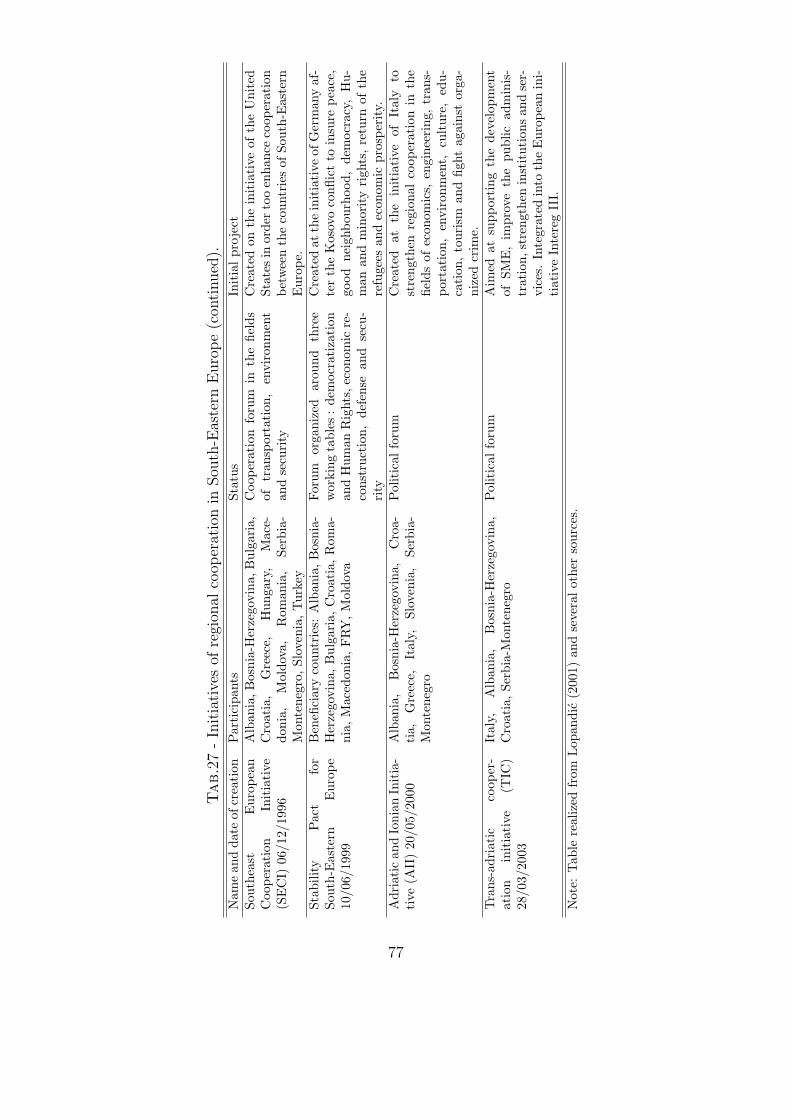
Tab.2

7-

Initia

tive

sof

regi

onal

coop

erat

ion

inSou

th-E

aste

rnE

uro

pe

(con

tinued

).N

ame

and

date

ofcr

eation

Par

tici

pant

sSt

atus

Initia

lpr

ojec

tSo

uthe

ast

Eur

opea

nC

oope

ration

Initia

tive

(SE

CI)

06/1

2/19

96

Alb

ania

,Bos

nia-

Her

zego

vina

,Bul

gari

a,C

roat

ia,

Gre

ece,

Hun

gary

,M

ace-

doni

a,M

oldo

va,

Rom

ania

,Se

rbia

-M

onte

negr

o,Sl

oven

ia,T

urke

y

Coo

pera

tion

foru

min

the

field

sof

tran

spor

tation

,en

viro

nmen

tan

dse

curi

ty

Cre

ated

onth

ein

itia

tive

ofth

eU

nite

dSt

ates

inor

derto

oen

hanc

eco

oper

atio

nbe

twee

nth

eco

untr

ies

ofSo

uth-

Eas

tern

Eur

ope.

Stab

ility

Pac

tfo

rSo

uth-

Eas

tern

Eur

ope

10/0

6/19

99

Ben

efici

ary

coun

trie

s:A

lban

ia,B

osni

a-H

erze

govi

na,B

ulga

ria,

Cro

atia

,R

oma-

nia,

Mac

edon

ia,FRY

,Mol

dova

Foru

mor

gani

zed

arou

ndth

ree

wor

king

tabl

es:

dem

ocra

tiza

tion

and

Hum

anR

ight

s,ec

onom

icre

-co

nstr

uction

,de

fens

ean

dse

cu-

rity

Cre

ated

atth

ein

itia

tive

ofG

erm

any

af-

ter

the

Kos

ovo

confl

ict

toin

sure

peac

e,go

odne

ighb

ourh

ood,

dem

ocra

cy,

Hu-

man

and

min

ority

righ

ts,re

turn

ofth

ere

fuge

esan

dec

onom

icpr

ospe

rity

.A

dria

tic

and

Ioni

anIn

itia

-tive

(AII

)20

/05/

2000

Alb

ania

,B

osni

a-H

erze

govi

na,

Cro

a-tia,

Gre

ece,

Ital

y,Sl

oven

ia,

Serb

ia-

Mon

tene

gro

Pol

itic

alfo

rum

Cre

ated

atth

ein

itia

tive

ofIt

aly

tost

reng

then

regi

onal

coop

erat

ion

inth

efie

lds

ofec

onom

ics,

engi

neer

ing,

tran

s-po

rtat

ion,

envi

ronm

ent,

cultur

e,ed

u-ca

tion

,to

uris

man

dfig

htag

ains

tor

ga-

nize

dcr

ime.

Tra

ns-a

dria

tic

coop

er-

atio

nin

itia

tive

(TIC

)28

/03/

2003

Ital

y,A

lban

ia,

Bos

nia-

Her

zego

vina

,C

roat

ia,Se

rbia

-Mon

tene

gro

Pol

itic

alfo

rum

Aim

edat

supp

orting

the

deve

lopm

ent

ofSM

E,

impr

ove

the

publ

icad

min

is-

trat

ion,

stre

ngth

enin

stitut

ions

and

ser-

vice

s.In

tegr

ated

into

the

Eur

opea

nin

i-tiat

ive

Inte

reg

III.

Not

e:Tab

lere

aliz

edfr

omLop

andi

c(2

001)

and

seve

ralo

ther

sour

ces.

77

Table 28: List of the countries of the sample

Rest of the European Central and Eastern South-Easternworld Union European countries Europe

(World) (EU) (CEE8) (SEE7)Algeria Austria∗ Czech Republic SEE5:

Argentina Belgium and Luxembourg Hungary AlbaniaAustralia Denmark Poland Bosnia-Herzegovina

Brazil Finland∗ Slovakia CroatiaCanada France Slovenia MacedoniaChina Germany Estonia Serbia-Montenegro

Colombia Greece Latvia SEE2:Egypt Ireland Lithuania Bulgaria

Ecuador Italy RomaniaHong Kong NetherlandsIndonesia Portugal

Israel Sweden∗

Japan SpainMorocco United KingdomMalaysiaMexicoNorway

New-ZealandPeru

PhilippinesRussia

SingaporeSouth KoreaSwitzerlandThailandTunisiaTurkey

United StatesVenezuela

Notes: * denotes countries which entered the EU in 1995. The 8 CEE countriesare not included in EU group because they were not members during the timespan of this study.

78

Table 29: CHELEM-CEPII sectoral classification of international trade, 10 sectors.

Code Secteur Included productsB Construction Products BA + BB + BCC Basic Metals CA+ CB + CCD Textiles DA + ... + DEE Wood Paper EA + ... + EEF Metal Products FA + ... + FWG Chemicals GA + ... + GIH Mining HA + HB + HCI Energy IA + IB + IC + IG + IH + IIJ Agriculture JA + JB + JCK Food Products KA + ... + KI

79

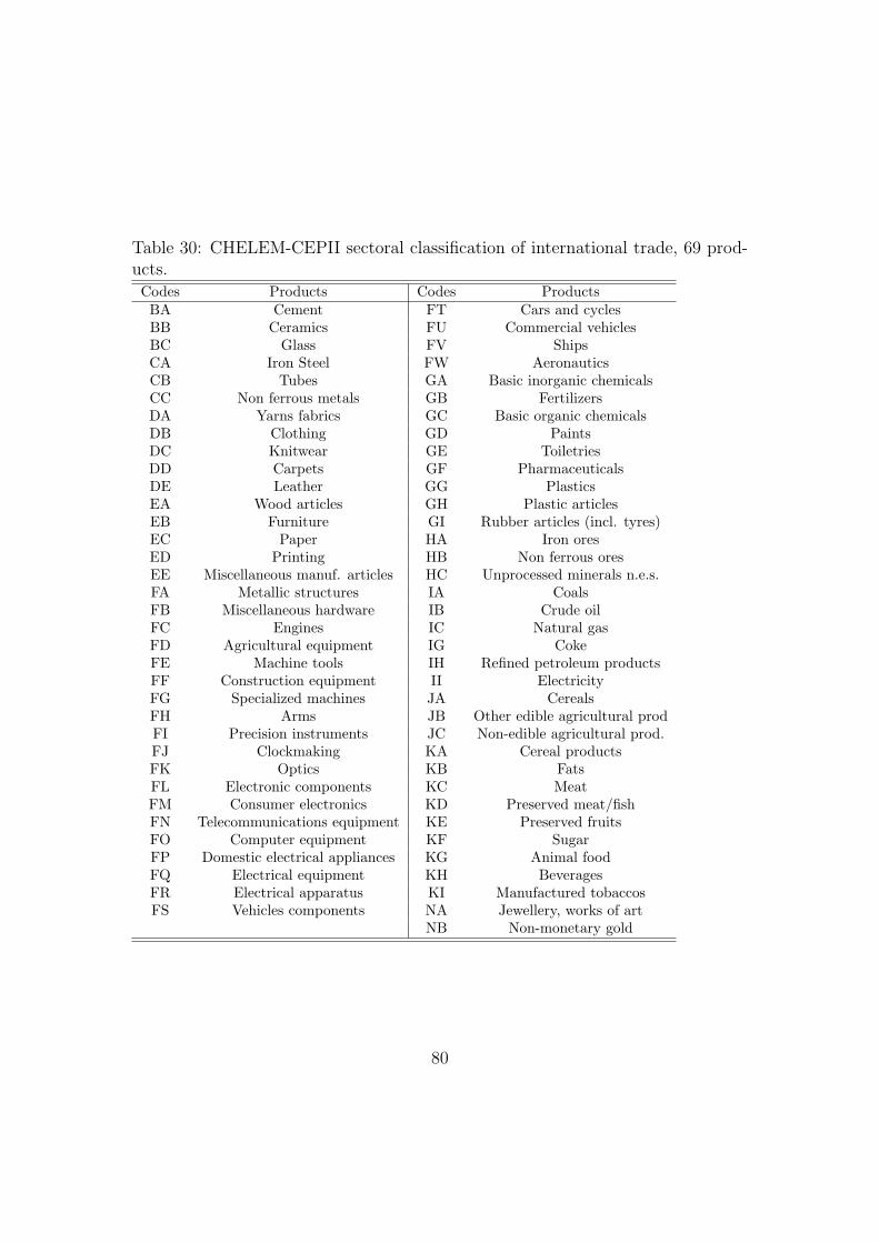
Table 30: CHELEM-CEPII sectoral classification of international trade, 69 prod-ucts.Codes Products Codes ProductsBA Cement FT Cars and cyclesBB Ceramics FU Commercial vehiclesBC Glass FV ShipsCA Iron Steel FW AeronauticsCB Tubes GA Basic inorganic chemicalsCC Non ferrous metals GB FertilizersDA Yarns fabrics GC Basic organic chemicalsDB Clothing GD PaintsDC Knitwear GE ToiletriesDD Carpets GF PharmaceuticalsDE Leather GG PlasticsEA Wood articles GH Plastic articlesEB Furniture GI Rubber articles (incl. tyres)EC Paper HA Iron oresED Printing HB Non ferrous oresEE Miscellaneous manuf. articles HC Unprocessed minerals n.e.s.FA Metallic structures IA CoalsFB Miscellaneous hardware IB Crude oilFC Engines IC Natural gasFD Agricultural equipment IG CokeFE Machine tools IH Refined petroleum productsFF Construction equipment II ElectricityFG Specialized machines JA CerealsFH Arms JB Other edible agricultural prodFI Precision instruments JC Non-edible agricultural prod.FJ Clockmaking KA Cereal productsFK Optics KB FatsFL Electronic components KC MeatFM Consumer electronics KD Preserved meat/fishFN Telecommunications equipment KE Preserved fruitsFO Computer equipment KF SugarFP Domestic electrical appliances KG Animal foodFQ Electrical equipment KH BeveragesFR Electrical apparatus KI Manufactured tobaccosFS Vehicles components NA Jewellery, works of art

NB Non-monetary gold

80