the weakly coupled yukawa2 field theory: … p(4>)2, pa = e~ua where t/a = /a : p() : d2x. one...
TRANSCRIPT
TRANSACTIONS OF THE
AMERICAN MATHEMATICAL SOCIETY
Volume 234, Number I, 1977
THE WEAKLY COUPLED YUKAWA2 FIELD THEORY:
CLUSTER EXPANSION AND WIGHTMAN AXIOMSi1)
BY
ALAN COOPER AND LON ROSEN(2)
Abstract. We prove convergence of the Glimm-Jaffe-Spencer cluster ex-
pansion for the weakly coupled Yukawa model in two dimensions, thereby
verifying the Wightman axioms including a positive mass gap.
I. Introduction. In [9], [10] Glimm, Jaffe and Spencer developed a powerful
method for studying the weakly coupled P(<f>)2 model. In this paper we shall
apply their "vacuum cluster expansion" of [9] to the Yukawa model in two
dimensions. This method is largely model independent and should be applica-
ble to any weakly coupled, superrenormalizable model based on functional
integration in boson "g-space". (For recent applications to the <b* model, see
Feldman and Osterwalder [6] and Magnen and Sénéor [13].) In the next
section we present a brief review of the cluster expansion, but the basic idea is
as follows: For a Euclidean field model with interaction in the region A c Rrf,
one expects the interacting measure to have the form
(1.1) dvK « pAdii.
Here dp. is the free boson measure with mass m0 > 0, i.e. the Gaussian
measure on Q - § '(Rd) with mean 0 and covariance C = (- A + m2.)-1; and
pA is a function of the fields in A that embodies the interaction. For example,
for P(4>)2, pA = e~UA where t/A = /A : P(<j>) : d2x. One wishes to show that
dvK decouples between distant regions exponentially in the distance. If the
model is local in the sense that
0-2) Pa,ua2 = Pa.Paj
for disjoint A, and A2, then the coupling in (1.1) is due only to the Gaussian
measure dp (C = (—A 4- m%)~x is a nonlocal operator). Instead of dp,
suppose we consider the Gaussian measure dp® with covariance C$ =
(-Aa + m2,)'1; here A$ is the Laplacian (d = 2 henceforth) with Dirichlet
boundary conditions on % = (Z2)*, the set of unit line segments (= bounds)
Received by the editors February 26, 1976.
AMS (MOS) subject classifications (1970). Primary 81A18; Secondary 47B10, 35J05.(') Research partially supported by the National Research Council of Canada and by USNSF
Grant GP-39048.(2) A. Sloan Foundation Fellow.
C American Mathematical Society 1977
1
License or copyright restrictions may apply to redistribution; see http://www.ams.org/journal-terms-of-use
2 ALAN COOPER AND LON ROSEN
joining lattice points in Z2. The measure d/xa completely decouples across
lines in % and hence by (1.2) so does dvA0 = pA dp®. The cluster expansion
consists of relating the measure of interest, dvA, to this exactly decoupling
measure, dvA0, by means of a perturbation expansion in the bonds in %.
We consider now the Yukawa model in two dimensions ( Y2) for interacting
bosons and fermions. At present there is not available a fermion integration
theory analogous to the boson functional integration on which to base the
cluster expansion. However, Seiler [22] recently established a rigorous version
of a formula of Matthews and Salam in which the fermions have been
"integrated out" with the result that the Euclidean Green's functions or
Schwinger functions of the Y2 model can be represented by a purely boson
integration with a measure of the form (1.1). The Matthews-Salam-Seiler
formula for the Schwinger functions for « bosons and m fermion-antifermion
pairs is as follows:
(1.3) SA(f, g,h) = Z-xj$(h)det S'(f„ g;, <¡>)pA dii
where
(a) / = (/i, • • • ,fm), g = (gi, • • •, gm) and h = (A„ ..., h„) are suitable
test functions (e.g. h} in S (R2), and./;, g, in S (R2) © § (R2));
(b) d¡i is the free boson measure on § '(R2) with mass mb > 0 and 0(A) =
n?_i<i>(/i/) where <j> is the free boson field;
(c) S'(fi, g/, <t>) = Up 0 - *K)~%gj)o where ("' Oo denotes the inner
product on %¡ = L2(R2) © L2(R2); X G R is the coupling constant; S0 is the
free two point Schwinger function for the fermions with mass mf > 0,
i - & + mf
(1.4) S0(x - y) = -i- / —-4 *»<*-*> d2?(2trf J p2 + mf
where p- = p0y0 + .p. y. in terms of p = (p0, p¿) and the 2 X 2 y-matrices y0
and y, (see [22]). K = KA is the operator with kernel
(1.5) KA(x,y) = S0(x- y)<t>(y)xA(y)
where Xa is the characteristic function of A. The determinant in (1.3) is the
m X m determinant of the matrix with elements S'(f¡, gy, <b).
(d)
(1.6) pA = detren(l - \KA) = det3(l - AK^exp^X^),
where
(1.7) det3(l - A) = exp[Tr(ln(l - A) + A + A2/2)j
and
(1.8) BA = \ :Tr(K2 + &K):,
License or copyright restrictions may apply to redistribution; see http://www.ams.org/journal-terms-of-use
YUKAWA2 FIELD THEORY 3
where K* is the adjoint of K as an operator on %¡ and : : denotes Wick
ordering with respect to dp;
(e) the partition function
(1.9) Z=fpAdp.
The above description (a)-(e) of (1.3) is only formal. For instance, it is not
clear what det3(l - XKA) or
(1.10) R = il-XKAyx
means, inasmuch as KA depends on the field ^ which takes values in S '(R2).
What Seiler did was to introduce momentum cutoffs so that each component
of (1.3) made sense, to perform appropriate renormalization cancellations,
and then to take the limit as the cutoff was removed. In this way he showed
that the integrand in (1.3) was indeed an integrable function of </>. Refine-
ments of Seiler's results and further developments based on (1.3) have been
obtained independently by McBryan [15], [16], [17] and by Seiler and Simon
[23], [24], [25]. We mention two of their results, but first some notation. Let
D = ip2 + m2)xl2 = (-A + w/)'/2 and let %a be the Sobolev space %a =
V-iD2^). Define X = %/2 © %/2 and /\m% to be the w-fold anti-symmetric tensor product of % with itself. It is not hard to show that
(1.11) det S'(J, gy, <b) = m\ TxAm%(/\mR • P)
where /\mR is the w-fold antisymmetric tensor product of the operator R
(see (1.10)) with itself and P is the projection operator on /\m% defined by
(1.12) P = Oí, -)A-3e*
where r, - D~% A • • * AD~% and xb - SQgx A • • • A S0gm. (In the
Appendix we have collected the various definitions and facts about /\m%
that we shall use.) Now define
(1-13) HVA(<p)=||Am*||PA
where || Am*ll is the norm of Am^ as an operator on /\m%. Then it is
shown in [16] and [24] that for any p < oo there are constants c, and c2
independent of m and A such that ("Linear Lower Bound")
0.14) IKaIU,) < cfV2|A|
where |A| is the volume of A. Note that the estimate (1.14) involves a
cancellation between poles of Am^ as a function of X and zeros of
det3(l — XK). This estimate is an important ingredient in obtaining bounds
on the Schwinger functions: McBryan [17] and Seiler and Simon [25] show
that if A -» oo through a sequence of rectangles then
(1.15) m^iJ^h^Kinlf^lg]^A-»oo
License or copyright restrictions may apply to redistribution; see http://www.ams.org/journal-terms-of-use
4 ALAN COOPER AND LON ROSEN
where | • |0 and | • |, are Schwartz space norms with |/|0 = II7LiU-lo etc-
At first sight the formula (1.3) for SA seems inappropriate for a cluster
expansion since the "interaction" is nonlocal: the price paid for integrating
out the fermions is that the "effective interaction", -logdetren(l - XK),
involves products of the boson field at different points in R2. Put differently,
(1.2) fails for pA defined by (1.6):
(1.16) Pa,ua2 * Pa,Pa2-
However, if we reinstate the fermi fields by going to the Osterwalder-Schrader
representation [18], then the interaction is certainly local and it makes good
sense (at least at the pre-estimate level) to base a cluster expansion on
inserting Dirichlet barriers in both the boson and fermion two point Green's
functions. One is therefore confident at the outset that the nonlocality (1.16)
cannot be a serious problem for a cluster expansion, provided of course that
one inserts Dirichlet barriers into the fermion "covariance" (1.4). We do so in
the following elementary way:
(1.17) S0(s; x,y) = Cf(s; x,y)(r+ mf) = (-iVy + mf)Cf(s; x,y),
where s is a multiparameter in [0, 1]® measuring the strength of Dirichlet
barriers (see §11) and Cj(s; x,y) is defined in precisely the same way as the
boson covariance (see (11.15)) except that mb is replaced by mf. Since
fr = — i V is a local operator S0(s) decouples across a Dirichlet barrier just as
Cf(s) does. With this choice, the Y2 theory does "decouple at í = 0", as we
explain in §111 where we formally derive the Y2 cluster expansion.
In §IV we prove convergence of the Y2 cluster expansion. As is to be
expected, some vestige of nonlocality remains in the sense that the cluster
expansion produces nonlocal polynomials of the form
}w(xl,..., Xj^x^)... <b(Xj) dx; however the nonlocality is exponentially
small in the sense that the kernels w(x{,..., Xj) are exponentially small in
the distance between the x/s. The estimates required for convergence are
established in §VI and §VII. For example, in §VII.4 we extend the linear
lower bound (1.14) to the j-dependent theory. For P(<b)2, estimates on Lp
norms of B^C^s; x, y) are critical [9], where, for y a finite set of bonds in ©,
9Y = Hbeyd/dsb. It is clear from definition (1.17) that we must consider
analogous bounds involving spatial derivatives as well. It turns out that all the
estimates in this paper can be reduced to estimates on the second mixed
partial (d2/dx¡dy)dyC. §VI is devoted to such estimates and in a certain
sense is the technical heart of the paper. Instead of a Wiener integral
representation as in [9], [28], we employ elementary techniques from the
theory of partial differential equations.
As in the case of P($)2, the Wightman axioms [30] for weakly coupled Y2
(except asymptotic completeness) are an immediate consequence of the
License or copyright restrictions may apply to redistribution; see http://www.ams.org/journal-terms-of-use
YUKAWA2 FIELD THEORY 5
convergence of the cluster expansion. In §V, we sketch the proofs of the
following results:
Theorem 1.1. If \X\/mb and \X\/mj are sufficiently small then:
(a) The infinite volume Schwinger functions S (f, g, h) = limA_R2SA(/, g, h)
exist.
(b) The S(f, g, h) satisfy all of the Osterwalder- Schroder axioms [19] includ-
ing exponential decoupling. Hence the corresponding relativistic theory satisfies
the Wightman axioms including a positive mass gap.
In our development of the Y2 cluster expansion we have tried to conform
as closely as possible to the version of the expansion in the Erice lectures [9].
However there are some additional features worth noting here:
(a) The integrand, as well as the Gaussian measure, depends on s. Deriva-
tives in s of the integrand ("fermion derivatives") lead to terms with a
different structure than derivatives of the measure ("boson derivatives"); in
order that we can treat both types of derivatives in a uniform way we find it
convenient to introduce dummy boson fields to replace those that have been
differentiated.
(b) We find it more convenient to use s-Wick ordering matched to the
measure dpC(Sy
(c) In order to take advantage of the linear lower bound (1.14) it is
important after each step in the cluster expansion to collect together certain
terms in such a way as to preserve the form (1.11).
(d) The nonlocality referred to above, while not a serious problem, affects
the combinatorics of the cluster expansion. In particular, a set of bonds y
may have from 1 to 6 associated localizations, instead of exactly 2 as in the
P (<f>)2 case.
(e) As remarked above, the convergence of the cluster expansion depends
on Lp bounds on (d2/dxidyJ)dyC. Although dyC(s; x,y) has only mild
singularities (i.e. logarithmic) asxorv approaches a bond and hence is any
Lp, the singularities of (32/3x/9y/)81'C are more severe and make it a delicate
question as to what Lp space (o2/'dxi'èyJ)VC belongs to (see Theorem VI. 1).
(f) To deduce convergence of the cluster expansion based on the unit lattice
Z2, we have to take |X| small as well as mb and ms large. The reasons for this
are (i) to compensate for positive powers of mb and mf introduced by the Lp
estimates referred to in (e); and (ii) to bound the partition function for a unit
square A away from zero as in [9]. The conclusions of Theorem 1.1, however,
are extended by a scaling argument to all values of X, mb, mf for which the
dimensionless ratios X/mb and X/mf axe sufficiently small. It is also possible
to develop a convergent cluster expansion for any given value of X (see the
Remark following Theorem V.l) provided one chooses mb and m¡ sufficiently
License or copyright restrictions may apply to redistribution; see http://www.ams.org/journal-terms-of-use
6 ALAN COOPER AND LON ROSEN
large and the basic lattice spacing sufficiently small.
The following miscellany of remarks and conventions is mostly notational:
(i) We denote the twice subtracted determinant (see (1.7)) by det3 as in [15]
and [24] instead of by det(2) as in Seiler's original paper [22].
(ii) As noted in [25], the combination (1 - XK) and not (1 + XK) as in
Seiler [22] corresponds to the Yukawa Hamiltonian with coupling constant
+ X.(iii) We shall often assert that something is true uniformly in the bare
parameters; it is to be understood that the bare parameters lie in the region
{(X, mb, mf)\ \X\ < l,mb> I, mf > I).(iv) For notational convenience we shall usually set mb = mf= m0.
(v) X will be suppressed in most of the formulas until the proof of
convergence when it will be required.
(vi) Following standard convention, we shall usually omit spin indices and
confuse %a © %a with %a.
(vii) Although we have stated the Matthews-Salam-Seiler formula for the
scalar theory, all of our results hold for the pseudo-scalar theory obtained by
inserting an ry5 in the definition of K: K = Sniy54>xA.
As we were completing this manuscript we received a preprint from J.
Magnen and R. Sénéor [14] who have obtained the same results as we do but
by a rather different approach. We mention also that D. Brydges [2] has
developed a cluster expansion in the Hamiltonian framework for a fermion
field \p moving in an external field <b via the interaction \¡ñf/c¡>.
Acknowledgements. We wish to thank Joel Feldman, Peter Greiner, Ira
Herbst, Elliott Lieb, Barry Simon, and Tom Spencer for useful conversations.
II. Review of the Glimm-Jaffe-Spencer cluster expansion. For the reader's
convenience we outline in this section the basic ideas, definitions, and steps in
the cluster expansion of Glimm, Jaffe, and Spencer [9]. Our review is no
substitute for the presentation in [9] but we hope that it makes this paper
reasonably self-contained. Although the following discussion applies strictly
only to P(<b)2, we have tried to phrase matters in a model-independent way.
So consider the situation described in (1.1) and let (A}A = fA(<b) dvA
denote the expectation of a function A of the Euclidean fields and let
&A(A) = (A)A/Z(A) denote the normalized expectation where Z(A) = <1>A
is the partition function. The purpose of the cluster expansion is to prove
exponential decoupling or clustering of the form
(HO SA(AB) - SA(A)&A(B) = 0(e-^A^).
Here the constant m is independent of A, A, B but depends only on the bare
parameters (masses, coupling constants) and is positive for suitable values of
these parameters; d(A, B) is the distance between the regions where the
License or copyright restrictions may apply to redistribution; see http://www.ams.org/journal-terms-of-use
YUKAWA2 FIELD THEORY 7
functions A and B axe localized. It is worth pointing out that clustering such
as (II. 1) with m > 0 leads in a straightforward way to the existence of the
infinite volume limit limA_00SA [8, Theorem 2.2.2].
It is no loss of generality in (II. 1) to suppose that A and B axe each
localized in unit squares A,, and AB in R2 \ © where $ = (Z2)*. We also take
A to be a union of unit squares. Furthermore we may suppose that each of A
and B satisfies (for the various boundary conditions used below)
01.2) &A(A) = &A(B) = 0
for the general case can always be reduced to this one by a suitable
"doubling" of the theory (see [9, Theorem 2.1]). For such A, B the goal (II. 1)
simplifies to
(II.3) &A(AB) = e(e~MB)).
If instead of < • >a an<i ^a we were to consider < • >A0 and €>A0 corre-
sponding to the measure dvA0 with D B.C. (Dirichlet boundary conditions) on
all the bonds in % (see §1); then we would have exact decoupling between
lattice squares. Thus, for AA =£ AB,
by (II.2) for D B.C.The cluster expansion proof of (II.3) now consists of relating SA to SA0
and showing that
(114) &A(AB ) - &Afi(AB ) - 0 (e —"•* >).
Considering the unnormalized expectations, one goes from (AByA0 to
(AByA by "turning on" the couplings across bonds in such a way as to
exhibit the smallness of the differences. This is accomplished as follows. With
each bond b E © we associate a parameter sb = 0 or 1 where sb = 0
corresponds to D B.C. on b and sb ■ 1 corresponds to full coupling across b,
i.e. no B.C. on b (later sb will range throughout the interval [0, 1]). For any
value of the multiparameter s = (sb)be<Sl we have B.C. intermediate between
(AByAfi = <^5>Ai_0 and (AByA =\AByA^^x and we denote the corre-
sponding expectation by (AByA¿. For any function f(s), b E % and set
Tc©,let
(8bf)(s)=m\si-l-m\St-v
(IL5) // \ \(5 r/)w = ((nr5ft )/)(.).
Then we have the (formal) identity
01.6) /(l)-/(0)= II (5r/)(0)re®
License or copyright restrictions may apply to redistribution; see http://www.ams.org/journal-terms-of-use
8 ALAN COOPER AND LON ROSEN
where the sum is over finite nonempty sets T. Note that 8Tf(s) is independent
of the values of sb, b ET; hence setting s = 0 in the summand in (II.6) gives
D B.C. only on Ve = % \ T. The expansion (II.6) corresponds to the Mayer
expansion from statistical mechanics. Its usefulness, for suitable functions /,
depends on the fact that, as a multiple difference of order |r|,
(11.7) 0Tf(0)&e-cM
where the constant c -♦ oo as m0 -» oo (see (11.20) below). If we had gone
from/(0) to/(l) via single differences, we would have obtained a sum with
"fewer" terms but would have lost the important decay (II.7).
As remarked after (II.6) 5^(0) has D B.C. on Ve: we regard the line
segments in Ve as barriers and those in T as bonds. With this viewpoint, T
gives a decomposition of R2 into connected components: R2 \ Ve = \JXj
where the Xj are disjoint. Returning to the "proof" of (II.4) we have from
(II.6) that
01.8) (AB\A-(AB)At0= 2 ST(AB)Afire®
where Ôr(AB\0 = o\AB)A¡,.0. If A,, * AB, (AB}Afi = 0. In fact, by
(II.2) the summand ÔT(AB}A0 will vanish unless T connects à.A and AB within
one connected component X,. For this to be the case T must be sufficiently
large, i.e. |r| > d(A, B). Therefore we expect that by (II.7) each term in (II.8)
is «exp[-cd(A, B)].
Now the above intuitive remarks cannot lead to a proof that (AB}A is
0^e-md(A,B)^ uniformly in A since (AB)A is unnormalized. To fashion a
proof from the above ideas it is necessary to divide by Z(A) and to effect a
cancellation. This is accomplished by a partial resummation of the expansion
(11.8) as follows. In the sum in (II.8) let T = T, u T2 where Tx connects A^
and AB; i.e., if X is the single component of R2 \ P7 containing â.A and AB,
then r, = T n int X. We obtain
(II.9) Sôr<^>A0=2 2 2 8sTluT1<AB)Afi
re« x r,cint^r2cJfc
where the X and T, sums satisfy
(i) X is a finite, closed, connected union of lattice squares
(11.10) containing A^ and AB,
(ii) T c % n int X is such that X ~ T\ is connected.
Now (T, u Tj) n 3* = 0 so that 5r'UI"2<^i9>A>0 decouples across ZX:
(11.11) 8^(AB\0= 8^(AB)AnX^(l)ArXtfi.
By (a slight generalization of) (II.6),
License or copyright restrictions may apply to redistribution; see http://www.ams.org/journal-terms-of-use
YUKAWA2 FIELD THEORY 9
(11.12) 2 Sr2<l>An^o=<1>An^l-iin^-Omx = Z3^(A~A'),T2gXc
the partition function with interaction in A ~ X and D B.C. on dX. Therefore
by(II.8Hn.l2)
<^>a-2 2 sr>(AByAnxfizdx(^~x)X r,cintJf
so that, dividing by Z(A),
Z3^(A~Z)
(11.13) &A(AB)= 2 z(A) ^'^Wo
where the sums over X, Tx satisfy conditions (11.10) above.
The identity (11.13) is the desired cluster expansion for &A(AB). One
deduces (II.4) by proving that the summand in (11.13) is bounded by
(11.14) e(e-cM+dW),
the e-clr'l arising from the multiple difference 5r' and the ed^ from the ratio
Zdx\Z and the exp(0(|A n X\)) behaviour of an expectation < • >An^. Here
d is uniformly bounded in the bare parameters whereas c -» oo as m0 -» oo.
But by (ii) of (11.10), T, must fill out X; more precisely, (ii) implies that
|r,| > 1*1 - 1 so that (11.14) is bounded by 0(e-(f-d)m). Since there are at
most 0(eQaX9)M) terms in (11.13) with a fixed value of \X\ [9, Proposition
5.1], we obtain
|SA(,L3)|<0 2 e-<c-d-XnX9)W<e(e-md^B))
\X\>d(A,B)
where m -» oo as m0 -» oo.
This concludes our "intuitive" description of how the cluster expansion
leads to exponential decoupling. We next wish to recall some definitions from
[9]. If T c ©, let Cr = (- Ar + ml)~x where Ar is the Laplacian with D B.C.
on the bonds in T. In order to interpolate between C^ = (—A + m2,)-1 and
C$ = (-Aa + ml)~x, we let the parameters sb range through [0, 1] and we
define the covariance
(11.15) C(s)= 2 n sb n (i - sb)re® Uer ¿er
In particular, C(0) = C9 and C(l) = Cr
We denote the Gaussian measure corresponding to C(s) by dpc^ or dps,
and the interacting measure in volume A by dvAs = pA¿ dps. For P(^>)2 the
factor pAi may be chosen to be independent of s, i.e. pA = e~u* =
exp(—fA:P(tp): d2x) and for this reason we assume that we are dealing with
P(<t>)2 for the rest of this section. (For the definition of pA^ in Y2, see the next
License or copyright restrictions may apply to redistribution; see http://www.ams.org/journal-terms-of-use
(ine) í(r) = r(,)={^
10 ALAN COOPER AND LON ROSEN
section.) The j-dependent partition function and (unnormalized) Schwinger
functions are
Z(A, s) =jdvAt„ ZS(A, S) -/*(/,) ... <K/„) dvAj,
where each test function f¡ is assumed to be smooth and localized in a lattice
square.
In order to expand F = Z or ZS as in (II.6) we must verify that F(s) is
regular at oo, i.e. if TV® through finite subsets, then F(s(T))-> F(s) for
each s, where
bel,
6 er.
In order to carry out the factorization as in (11.11) we must next verify that/
decouples at s = 0, i.e., if the D barriers in rc decompose R2 into a disjoint
union
(11.17) R2 ~ Tc = U Xj
then
(LUS) F(A, s(T)) = HF(A n Xj, s(T n Xj)).j
Given that F is regular at oo and decouples at s = 0 we can obtain a
convergent expansion as in (11.13). For S (A) = S (A, s = 1) we resum over
the components in (11.17) that do not meet the set X0 = U,- supp^- and the
resulting expansion is, just as in (11.13),
_ ZBX(A~X) „(11.19) s(A)= 2 "*; Vzs(An*,o)
(Ar,r)eS ^lA*
where the set S = S (X0) is defined by
§ = {(X, T)\X a finite union of closed lattice
squares with X0 c X; T c ® n int X is such that each
component of X ~ Ve meets X0 ).
There are three estimates involved in analyzing (11.19) as indicated in the
discussion of (11.13) above. The main one is Proposition 5.3 of [9]:
I. There is a constant c, < oo (uniformly in the bare parameters, X, and
|r|) and a norm |/| on test functions such that
(11.20) \8VZS(X, 0)| < e-«ITI+e>M|/|
where c -> oo as m0 -» oo.
The second estimate is on the ratio of partition functions: for sufficiently
large m0 there is a constant c2 < oo (uniformly in A, A" and the bare
License or copyright restrictions may apply to redistribution; see http://www.ams.org/journal-terms-of-use
YUKAWA2 FIELD THEORY 11
parameters) such that
01-21) \Zdx(A~X)/Z(A)\<ec>W.
As shown in §6 of [9], (11.21) follows from an appropriate cluster expansion
for Z ("Kirkwood-Salsburg equations"), a bound on Z analogous to (11.20),
and the following estimate:
II. Let Z3ii(A) be the partition function for a unit square A with D B.C. on
3A. For sufficiently small |X| and sufficiently large m0,
(11.22) 1<|2T3A(A)|.
The third estimate is a combinatorial one:
III. The number of terms in (11.19) with a fixed value of 1*1 is bounded by
Obviously, this last estimate is model independent. To summarize: for any
model the convergence of the cluster expansion reduces to proving (the analogue
of) estimates I and II.For the remainder of this section we discuss the method of proof of I. The
first step is to apply the fundamental theorem of calculus to 8T; i.e.
(11.23) 8TZS(0)=[ dTZS(o)d^oJ0<o<T(\)
where 3r = ITier3/3o-¿, and where, according to (11.16), the integration in
(11.23) extends over the region ob E [0, 1], b E T. But one has a simple
formula for ddpC(s)/dsb, namely [4]:
<IL24> ~k ÍG (*> *"« = Ï /( f " A*)G *"where
(1L25) (if• A*)G -// f <s;*•»mkf) ""*■The formula for higher derivatives follows from the product rule:
(11.26) dT[G(<t>)dpcU)= 2 f U \(VC-\)Gdpc,s)J lEí(r)'' ye» *
where WÇT) is the set of all partitions of T. From (11.23) and (11.26) we obtain
(11.27) 8TZS(X, 0) = 2 f d^s (dpsU \ VC-^(X)e-uMw<=<3'(r)J J yew l
where O(X) = IL;:supPícA.<í>(.¿).
Now the derivatives A^ in (11.27) produce a sum of products of local
polynomials : Q (<t>(X)): brought down from the exponential e~um. There are
thus a large number of terms in (11.27), for two distinct reasons:
License or copyright restrictions may apply to redistribution; see http://www.ams.org/journal-terms-of-use
12 ALAN COOPER AND LON ROSEN
(Bj) The number of terms ^(F)! in the sum over partitions is large, of the
order |r|lrL
(Bj) The number of terms resulting from differentiations A^ is large, of the
order |r|'r'; moreover, the total degree of the polynomial brought down is of
the order |r|, which results in a number singularity which could be of the
order |r|lrL
The only hope for controlling these singularities lies with the 8YC's. In fact,
dyC(x, y) is small for two (essentially) distinct reasons:
(G,) dyC(x,y) becomes exponentially small as y becomes large.
(G;¡) dyC(x,y) becomes exponentially small as x or y gets far from any
bond in y.
Fortunately, (G,) controls (B,) and (Gj) controls (Bj). The intuitive ex-
planation of the latter is this: given x e R2 there cannot be too many y's near
x and consequently by (G2) only a small number of the ¿5/5<f>(;c)'s are
significant at x. Hence, locally the number of terms and the degree of the
polynomial ("local number singularities") are effectively bounded indepen-
dently of |r|.For precise statements of (G,) and (G2) we quote Propositions 8.1 and 8.2
from [9], but first some more notation: Let Ay be the lattice square whose
lower left corner is at j E Z2. We let x, = Xà denote the characteristic
function of A,, and we define the distance
(11.28) d(y,j) = max[dist(6, A,.) + dist(Z>, AJ].
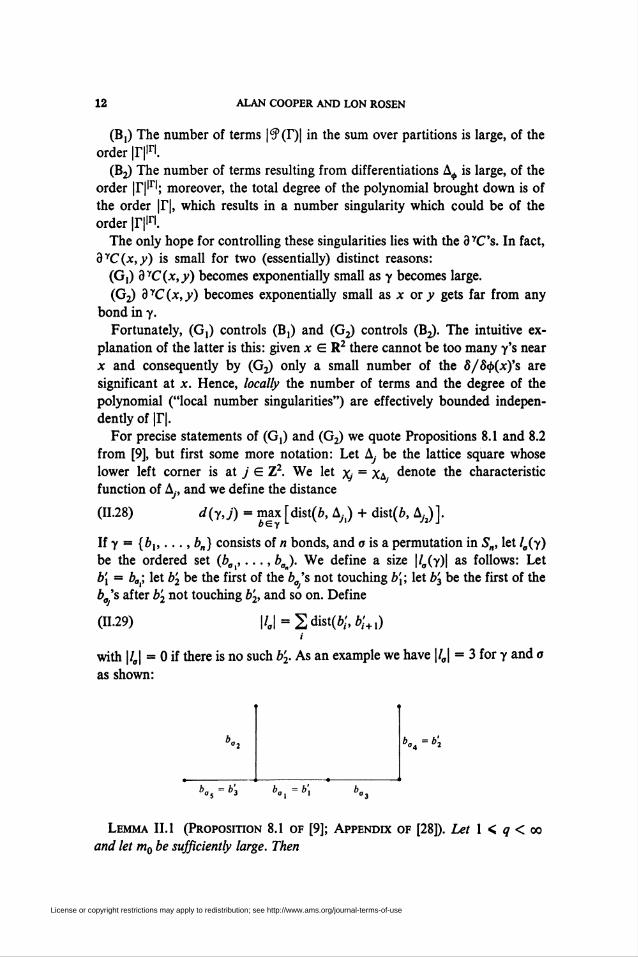
If y = {£>„ ... ,b„) consists of n bonds, and a is a permutation in Sn, let /0(y)
be the ordered set (ba , ..., b0). We define a size |/0(y)| as follows: Let
b\ «■ ba; let b'2 be the first of the b0's not touching b\; let b'3 be the first of the
bg 's after b'2 not touching b'2, and so on. Define
(11.29) IU = 2dist(ô;,è;+1)i
with |/„| = 0 if there is no such b2. As an example we have |/0| = 3 for y and a
as shown:
"•2 b„ =6;
b„ =b'3 ba = b\ ba5 1 ' Q %
Lemma II. 1 (Proposition 8.1 of [9]; Appendix of [28]). Let 1 < q < oo
and let m0 be sufficiently large. Then
License or copyright restrictions may apply to redistribution; see http://www.ams.org/journal-terms-of-use
YUKAWA2 FIELD THEORY 13
(11.30) Ito^Cj^< K4(q)Kiy%(y)möW2"exp[-mnd(y,j)/3]
where K4(q) and Kg are constants independent ofmQ and
(11.31) K6(y)= 2 e-m°My)i/3.oes„
Lemma II.2 (Proposition 8.2 of [9]). For m0 sufficiently large there is a
constant K-¡ independent of m0 such that
(11.32) 2 II K6(y) < e«*l.ve9(X) yE»
Here, in barest outline, is how the proof goes that G} controls By The
analogous steps for Y2 require some modifications and will be explained more
fully in §IV:
Insertion of localizations. In order to estimate the number of terms in (11.27)
as well as the local number singularities A/(A), i.e., to control (Bj), and to take
advantage of (G2), we introduce a partition of unity for each local polynomial
brought down from the exponential. This amounts to the same thing as
writing
(11.33) dyC = 2^,9YC^ ^2 *yC(jy)J-, h
where jy = (jyA,jyt2) runs through Z4. The sum over j = (jy) is pulled to the
outside and for a fixed value of j, one estimates the other sums.
Estimates on Q-space integrals. Such estimates lead to a product of factors:
the Gj factor HySJ\dyC(Jy)\\L,; the typical boson factor ILJVXA)!; and to alinear lower bound factor e0(-\x\\
Counting. One introduces M (A) as the number of 8/8<b's localized in A.
Both the local number singularity factor ITAiV(A)! and the number of terms
(B2) are estimated by e0('r|)(IIM(A)!)^ for some ß depending only on the
degree of the polynomial.
(G,) controls (B,). This is just an application of Lemma II.2.
(GÍ) controls (B2). The (G2) factor is exp[-2Y/V(y,yY)/3] and the (B2)singularities have been replaced by
IlM(A)!^<expice2M(A)1+e|
for any e > 0. A geometric argument that
01.34) 2 M (A)3/2 < const( 2 d(y,jy) + \T\)
shows that (G^ controls (B^ for sufficiently large m0.
License or copyright restrictions may apply to redistribution; see http://www.ams.org/journal-terms-of-use
14 ALAN COOPER AND LON ROSEN
III. Cluster expansion for Y2: formalism. In this section we formally derive
the Y2 cluster expansion, the proof of convergence being given in §IV. As
described in the previous sections, a key point is to define the s-dependent
theory so that it decouples at s = 0. For Y2 it is also important to collect
terms in such a way as to preserve the fermion structure that enables us to
cancel poles with zeroes as in (1.14). For this reason, we shall write down the
expansion in a rather explicit way.
Our starting point is the Matthews-Salam-Seiler formula (1.3). We assume
without loss of generality that each of the functions in /, g and h is in
Schwartz space and has support in a unit square. As we have already stated in
(1.17) we shall obtain an i-theory which decouples at s = 0 (in the sense of
definition (11.18)) by replacing dp by dpC(s) and, in addition, by replacing the
fermion two-point function wherever it occurs by
(111.1) SQis; x,y) = C(s; x,y)(p-+ m0) - (-i*y + m0)C(s; x,y)
where C(s) is defined in (11.15). Note that we have set mb = m,= m0 and
that accordingly we use the same symbol C for both bosons and fermions.
The operator inequality C(s) < C(l) = C^ implies that (III.l) defines a
bounded operator S0(s) on L2(R2). Moreover, since
p-= -''(Yo9/9*o + Yi9/9*i)
is a local operator, S0(s), like C(s), decomposes across Dirichlet barriers; i.e., if
s = 0 on a set of barriers % which divides R2 into a disjoint union,
R2 \ % - U X¡, then
(111.2) S0(s)=es0(s)[L2(X,).i
The i-dependent objects corresponding to (1.5), (1.6), (1.10) and (1.12) are
defined in the obvious way:
(IIL3) K(s) = K(A,s) = S0(s)4>xA>
0II.4) R(s) = (l-XK(s))~l,
(ffl.5) P(s) = (-n,-)Am%t(s),
where \b(s) = S0(s)gx A • • • A S0(s)gm, and
p(s) = p(A,s) = detTen(x--M(A,s))
(III.6)= det3(l - XK(A, j))exp[ -X2B(A, s)]
where
(III.7) B - Bis) - B(A, s) - i [:Tr tf(A, s)\ + 8m2 :<¡>2(Xa):s],
the Wick subtractions being made with respect to C(s). Of course, (III.7) is
only formal, e.g. the relation :TrÄ'tÄ':= Sm2:d>2(xA): involves the infinite
License or copyright restrictions may apply to redistribution; see http://www.ams.org/journal-terms-of-use
YUKAWA2 FIELD THEORY 15
constant 8ml. What we really mean by (III.7) is the limit as an ultraviolet
cutoff is removed,
(III.8) B(s)=limBa(s),
where we introduce the cutoff a as follows: Let h(x) e C0°°({x| |x| < ¿})
with h > 0, fh(x) dx = 1 and h(x) = h(-x). Define h„(x) = a2h(ax). Then
the ultraviolet cutoff fermion propagator is defined by
0II.9) S0 o (s; x,y) = fs0 (s; x, z)h„(z - y) dz.
Set
Ka(A,s) = S%a(s)<?XK,
(IIL10a) . , ,„ ,,-.f *P f,_*
with
and
5w' = ^"/7à^)2
ha(p)=jeip\(x)d2x
(111.10b) Ba(A, s) = i [:Tr A. (A, s)\ + 8m^2(xA):,].
In (VII.52) we prove the convergence of (III.8) in L2(djLtcw).
Combining the above definitions we define the partition function
(111.11a) Z(s)=jp(s)dric(,)
and the (unnormalized) Schwinger function, as in (1.3),
(III.1 lb) ZS (s) = J$ Tm (AmR (s) • P (s))p(s) ̂c(i)
where we have used (1.11) and introduced the notation
rm(-) = m!TrA-5C(.).
In §IV we shall show using estimates from §VII that the objects in (ULI 1) are
well defined. However a word is in order here about the meaning of an
expression like (III.4) for R (s). As in [22] we let Qp (%) denote the class of
compact operators A on DC with \\A\\P = Tr(A*Ay/2 < oo; and we let Gpq.,
denote the class of 6p(%)-valued functions A (<b) with
(111.12) \\A\\Ptq;=y d^AMl < oo.
Since 11^(5)1144., is finite (see (VII.27)), it follows that K(s) is a well-defined
compact operator in the class ß4(3C) for almost all <f> (w.r.t. ¿Pcm)- Thus for
each fixed <¡> (except in a set of measure zero) (III.4) is well defined as an
License or copyright restrictions may apply to redistribution; see http://www.ams.org/journal-terms-of-use
16 ALAN COOPER AND LON ROSEN
operator on % except for a countable set [X\X~X E o(K(s))). Of course this
set of X will depend on <f> and so it is quite possible that there is no X for
which (1 - A/if)-1 makes sense a.e. in <p. (We mention that Seiler [22] has
proved that for every X, (1 — XK)~ ' is well defined for ¿> in a set of positive
measure.) However we note that in (III.llb) the factor /\mR can be com-
bined with the det3(l - XK) to obtain a cancellation between the poles of
/\mR and the zeros of det3(l - XK). More precisely, by Proposition 5 of the
Appendix of [23], if A E ßp, then
(111.13) A -> B = Am(l - ^r'det^l - A)
is a continuous map from Qp to t(/\m%), the bounded operators on /\m%.
Accordingly we can define Am^det2(l - XK) by continuity in X even at the
values X E o(K)~x. It will turn out in the course of the cluster expansion that
the "operator" R (s) will always occur in a single jactor oj the jorm /\rR (s),
and consequently we shall freely use the above remarks to manipulate with
K(s) and R(s) = (1 — XK(s))~x as though they were well-defined bounded
operators on % jor all «p and all X. For notational convenience we shall set
X = 1 until the end of §IV at which point X will be resurrected.
With the above definitions and interpretation we now assert that ZS(s)
and Z(s) decouple at s = 0 (see (11.18)). For suppose that s = 0 on ®0 c
(Z2)* with R2 ~ % = U X, a disjoint union. Let K = K(A, s) and K¡ =
K(A¡, s) where A, = A u X¡ so that K = 2Ä). Let %(X¡) be the subspace of
% consisting of functions with support in X¡. Then clearly K¡ = 0 on OC(A^) if
i g* j, Range K¡ c %(Xt) by (III.2), and so
(III.14a) K¡Kj = 0 ¡îi+j.
Define the operator R¡ = (1 - K¡)~ '. As explained above we may assume
that 1 & oiK) and 1 & o(K¡) for all i so that R = (1 - K)~x and R, axe
well-defined operators. It then follows from the above properties of Ä^- that
(III.14b) R = R¡ on3C(A-,.).
In addition we see from (III. 14a) that
det„(l - A') = det
= det
(1 - K)exp
n (1_K/)exp|£_j
= iIdetfl(l-Ai).t
Although it follows formally from (III.8) and (III. 10) that B decouples at
License or copyright restrictions may apply to redistribution; see http://www.ams.org/journal-terms-of-use
YUKAWA2 FIELD THEORY 17
J = 0,
(111.15) B(A,s) = '%B(Ai,s),I
the proof involves an ultraviolet cutoff argument which we postpone until
§VII.5. Using (111.14) and (111.15) we obtain from definition (III.6):
011.16) p(A,s) = Hp(Ak,s)k
in contrast to the nonlocality (1.16).
The trace term in (III. 1 lb),
Tm((AmR(s))P(s)) = detydf, R(s)S0(s)gj)L2),
also factors. Since each test function f¡, gJy h¡ is localized in a unit square it
must also be localized in one of the A^'s.By (III.2), if supp gj c Ak then
supp SQ(s)gj c Ak and so, by (HI. 14b),
R(s)S0(s)%-Rk(s)S0(s)gj
also has support in Ak. Consequently,
AiJ^(fi,R(s)S0(s)gJ)Ll= f(¿ *$>(')*) if supp/and supp gycA„
10 otherwise.
We see that, after a suitable relabeling of the rows, the matrix Ay decomposes
into blocks A¡-k) associated with the various regions Ak. Obviously det Ay « 0
unless these blocks are square, i.e. unless the same number (mk) of/'s as gy's
have support in each Ak. We also have the factorization
Tm((AmR(s))P(s)) = det,4, = ± ndet4«
011.17) „= ±nr^((A^)P0
where
Pk = {D-%A-- ■ AD-'/^.^o^A-- • AS0(s)gJmk
and/,,... ,fimk, gh,..., gjmk are the fs and g's with support in Ak.
If we insert (III. 16) and (HI. 17) into (III.ll) we obtain the desired decou-
pling since each p(Ak, s) and Rk is a function of the fields in Ak:
Lemma 111.1. ZS(s) andZ(s) decouple at s = 0.
For bounded A it follows easily from the results of §VII that ZS and Z are
"regular at oo" (defined before (11.16)). Thus the cluster expansions for ZS
and Z are generated exactly as for P(<#>)2 and we obtain for S:
License or copyright restrictions may apply to redistribution; see http://www.ams.org/journal-terms-of-use
18 ALAN COOPER AND LON ROSEN
(111.18) S(A) = 2 (±) Z*X{?Z X) fd^sdTZS(A n X, s(T)).(x,T)eS Z<A> J
Here the set S = §(*()) is defined following (11.19) in terms of the union X0
of the supports of the j¡, g¡, h¡; ZS(A n X, s(T)) is the unnormalized
Schwinger function with interaction in A n X and with the /■, g¡, h¡ localized
in A n X; and the ± sign arises from the permutations involved in the
factorization (III. 17) (it is unimportant for the purposes of this paper).
We must now "evaluate" the ¿-derivatives 3 r. Our calculations involve the
differentiation formula (11.24) which becomes, in the case of an i-dependent
integrand,
(111.19) |/G(^)%=/(f^f-^)*,Taking higher derivatives and using the fact that d/ds and 8/8<p commute,
we obtain
(111.20) dvÍGdps= 2 2 fÍLT J3*C-aV/G¿m,J T-Yb\jYj*<=<$(Tb)J \yev ¿ I
where Tb and Tj are disjoint subsets of T which we regard as index sets for
boson and fermion derivatives respectively. In §VII.6, we indicate the
rigorous justification of the formal relations (III. 19) and (111.20) for the class
of integrands G considered in this paper.
The boson and fermion derivatives are independent except for the follow-
ing convention. The integrand G will always contain the factor e~B (see
(III.6)) as well as factors brought down by differentiating B. Let bis; x, y)
denote the kernel of B, i.e.,
(111.21) Bis) =\jb(s; x,y):<b(x)<b(y):s dx dy.
Since we use matched Wick ordering (: :s denotes C(s) subtractions) we
obtain a cancellation between boson and fermion derivatives; e.g.,
(¿ + ïfA>-i/S(*!^)^)^):.**.The same cancellation occurs for higher ¿-derivatives. We accordingly adopt
the following convention. We drop the cancelled vacuum expectation terms
and collect the remaining terms in the form
(m.22) I Jdyb{s; x,y):<t>(x)<b(y):s dx dy.
Thus no term involving boson derivatives of B occurs in which the same
covariance kernel dYC(x,y) is integrated against each variable of b or dyb.
License or copyright restrictions may apply to redistribution; see http://www.ams.org/journal-terms-of-use
YUKAWA2 FIELD THEORY 19
From definition (III. 1 lb), and formula (111.20),
dTZS(s)= 2 2 Uii, n (L2^C-\)T=T„uT/ns9(r¡>)J Ye»4
(111.23)•^fTm(AmR(s)P(s))p(s).
We proceed to evaluate a typical fermion derivative (formally). Since R =
(1 - K)~x, we have
011.24) (d/ds)R = R(dK/ds)R.
Consequently,
3 A mr, _ V» / A /-ln\ A OR
011.25)
ys AmR - 2 (Aj~lR) A ^ A (Am-JR)
= dAm(R™)AmR
by (111.24), (A.5), and the definition (A.4) of the derivation d Am(-)- Since
(formally)
det3(l - K) = exp[Tr(log(l - K) + K + K2/2)]
we have
£de.3(l - K) - T,(-(l - *r)-f + f +*f )de«j(l - K)
--Tr(iKJ^)det3(l-ir).
Therefore
Cm,*) |._[Tr(^M) + f].
By (111.25) and (111.26)
±-sTm(AmR-P)P=\rm(dAm{R™)AmR-p)
+ Tm[AmR^)-Tm(AmR-P)
(111.27)
•H-2f)+fRecall that in the discussion following (III.13) we asserted that R always
occurs in a single factor of the form A'R> this fact being critical for our
control of the terms in the cluster expansion. Plainly this is not the case for
two terms on the right side of (111.27) and so we must effect a cancellation.
License or copyright restrictions may apply to redistribution; see http://www.ams.org/journal-terms-of-use
20 ALAN COOPER AND LON ROSEN
To this end we write R = RK2 + 1 + K so that
where
(111.28) A> = K2^£ and ^ = (1 + ^)^-
The two offending terms in (111.27) become
Tm(dAm(R™)AmR-p)-TmiAmR-P)Tx(RK2^))
= Tmi/\mR ■ Pd/\m(RAs)) - Tm(/\mR ■ P)TX (RAS)
+ TmiAmR-PdAm(Es))
(111.29) = - Tm+, ( AmR • P A RAS) + Tm iAmR • P dAm(Es ))
011.30) = -Tm+xiAm+iR-PAAs) + TmiAmR-PdAm{E,))
where in (111.29) we have used the trace formula (A. 12) and in (111.30) the
elementary identity (A.5). Combining (111.27) and (111.30) we obtain the basic
differentiation formula:
j-sTm(AmR-P)p=[-Tm+xiAm+iR-PAAs)
011.31) +7m(Am*-.rVAm(£J))
+ Tm[AmR^ )-Tm(AmR-P)^}p-
For G an operator on Am3C> we introduce the functional
(III.32) rm(G)=Tm(AmR-G)p
Then (111.31) can be written
j¡^(P) = rm(^)-rm+x(PAAs)
(III.33a)
+ rm(PdAmEs)-rm(P)f.
Each boson derivative gives an analogous formula. That is, if G(<b) is a
function of the fields taking values as an operator on Am3t\ then
-8^y-)TÁG) = TÁ^F))~Tm+l{GAAy)
(111.33b) 8B+ TmiGdAmEy)-rmiG)
8<b(y)
License or copyright restrictions may apply to redistribution; see http://www.ams.org/journal-terms-of-use
YUKAWA, FIELD THEORY 21
where
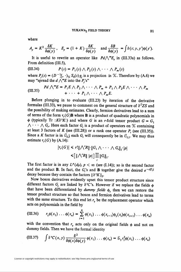
*> -KI m • E> -(1 + K) m ™d *w= Z**»*™*It is useful to rewrite an operator like PdAmEs in (HI.33a) as follows.
From definition (III.5),
(111.34) P (s) = Px (s) A P2 0) A • • • A Pm (s)
where Pj(s) = (D~% ■)% S0(s)gj is a projection in %. Therefore by (A.6) we
may "spread the d /\mE into the P/s"
PdAmE=PxE/\P2/\--- /\Pm + Px/\P2E/\--- /\Pm
(IIL35) +...+PlA...APmE.
Before plunging in to evaluate (111.23) by iteration of the derivative
formulas (111.33), we pause to comment on the general structure of 3 VZS and
the possibility of making estimates. Clearly, fermion derivatives lead to a sum
of terms of the form rr(G)B where B is a product of quadratic polynomials in
<j> (typically Tr :KdyK:) and where G is an r-fold tensor product G = (?,
A • • • A Gr. Here each factor G¡ is a product of operators on % containing
at least 3 factors of K (see (111.28)) or a rank one operator P¡ (see (111.35)).
Since a K factor is in (SjJ each G¡ will consequently be in (2,,. We may thus
estimate rr(G) by (A. 14):
K(fJ)|<r!||ArÄ||1(?,A---AC?r||,'|Pl
<[||Ar*|||p|]n>,||rI
The first factor is in any Lp(dri),p < oo (see (1.14)); so is the second factor
and the product B. In fact, the G,'s and B together give the desired e~c^
decay because they contain the factors ||9 YA||3.
Now boson derivatives evidently upset this tensor product structure since
different factors G, are linked by 3YC's. However if we replace the fields <b
that have been differentiated by dummy fields <by then we can restore the
tensor product structure so that boson and fermion derivatives lead to terms
with the same structure. To this end let ry be the replacement operator which
acts on polynomials in the field by
011.36) ry<b(Xl) . . . <b(xn) = 2 *(*,) - • • *(*.-i)*,(*M*,+,) • • • *(*„)i = i
with the convention that ry acts only on the original fields <j> and not on
dummy fields. Then we have the formal identity
(111.37) /a yc(x, y) s^l^ «*.) • • • <H*„) = VX*,) • • • <KO
License or copyright restrictions may apply to redistribution; see http://www.ams.org/journal-terms-of-use
22 ALAN COOPER AND LON ROSEN
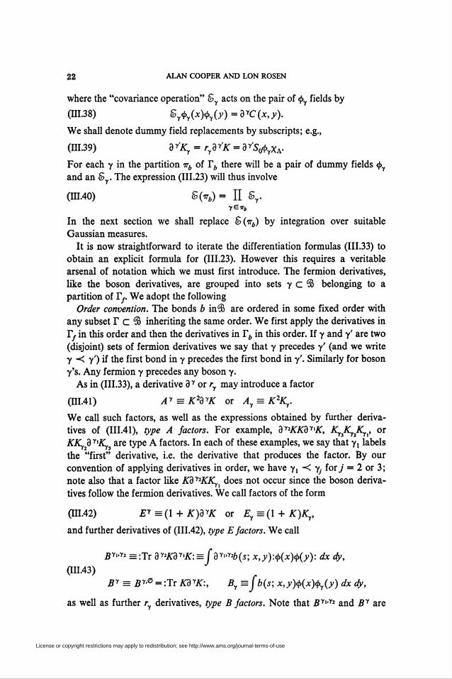
where the "covariance operation" Sy acts on the pair of <by fields by
(111.38) &y<by(x)<by(y)=dyC(x,y).
We shall denote dummy field replacements by subscripts; e.g.,
(111.39) 3 % - ryd*K - 9YS0<byXA.
For each y in the partition mb of Tb there will be a pair of dummy fields d>Y
and an Sy. The expression (111.23) will thus involve
(111.40) S(776)= n $ry^n
In the next section we shall replace S(77¿) by integration over suitable
Gaussian measures.
It is now straightforward to iterate the differentiation formulas (111.33) to
obtain an explicit formula for (111.23). However this requires a veritable
arsenal of notation which we must first introduce. The fermion derivatives,
like the boson derivatives, are grouped into sets ycS belonging to a
partition of Tj. We adopt the following
Order convention. The bonds b iniB are ordered in some fixed order with
any subset rc9 inheriting the same order. We first apply the derivatives in
Tj in this order and then the derivatives in Tb in this order. If y and y' axe two
(disjoint) sets of fermion derivatives we say that y precedes y' (and we write
y -< y') if the first bond in y precedes the first bond in y'. Similarly for boson
y's. Any fermion y precedes any boson y.
As in (111.33), a derivative 3 y or ry may introduce a factor
(111.41) Ay = K2dyK or Ay = K2Ky.
We call such factors, as well as the expressions obtained by further deriva-
tives of (111.41), type A jactors. For example, 3 y*KKd y>K, Ay^Ä^, or
KKydy'Ky} are type A factors. In each of these examples, we say that y, labels
the "first" derivative, i.e. the derivative that produces the factor. By our
convention of applying derivatives in order, we have Y! -< y, for y = 2 or 3;
note also that a factor like Koy2KKyi does not occur since the boson deriva-
tives follow the fermion derivatives. We call factors of the form
011.42) Ey=il + K)dyK or Ey=il + K)Ky,
and further derivatives of (111.42), type E jactors. We call
5y,.y2 = :Tr 0y2KotyK:= jdy>-y%(s; x,y):<b(x)<b(y): dx dy,
011.43)By = By# = :Tr KdyK:) By =jb(s; x,y)<b(x)<py(y) dx dy,
as well as further ry derivatives, type B jactors. Note that Byi,yi and By are
License or copyright restrictions may apply to redistribution; see http://www.ams.org/journal-terms-of-use
YUKAWA2 FIELD THEORY 23
well defined without the need for a mass term (see Corollary VII. 13). We
refer to the factors <p(A.) in $, and their derivatives, as type $ jactors, and the
factors Pj in (111.34), or their derivatives, as type P jactors.
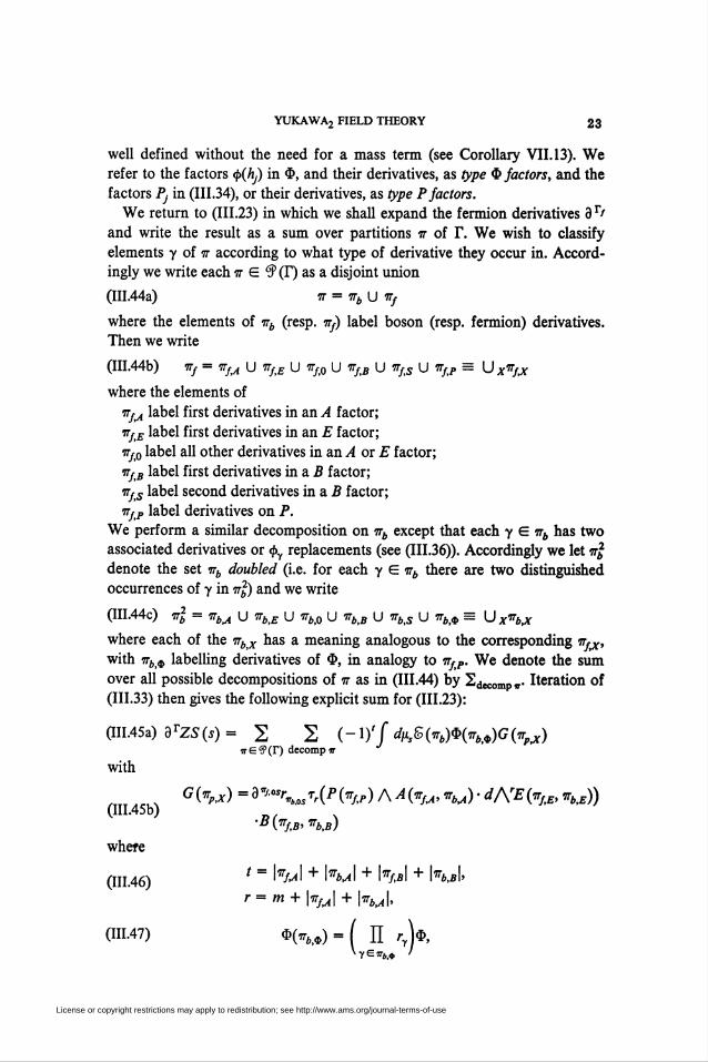
We return to (111.23) in which we shall expand the fermion derivatives 3 r'
and write the result as a sum over partitions it of T. We wish to classify
elements y of 77 according to what type of derivative they occur in. Accord-
ingly we write each 77 G $ (T) as a disjoint union
(III.44a) tr = irb U trf
where the elements of trb (resp. ttj) label boson (resp. fermion) derivatives.
Then we write
(III.44b) irf = tru U irftE U tt/>0 U wftB U vftS U vftP = U^
where the elements of
mJA label first derivatives in an A factor;
WfjE label first derivatives in an E factor;
•ttfß label all other derivatives in an A or E factor;
m¡B label first derivatives in a B factor;
TtfS label second derivatives in a B factor;
7iy p label derivatives on P.
We perform a similar decomposition on itb except that each y E mb has two
associated derivatives or d>? replacements (see (111.36)). Accordingly we let irb
denote the set trb doubled (i.e. for each y E irb there are two distinguished
occurrences of y in <nb) and we write
(111.44c) ml = ttm U wbfE U trbt0 U irb>B U trbS u irb,<¡> - Ux*bjc
where each of the ttbX has a meaning analogous to the corresponding it^,
with 77i>0 labelling derivatives of $, in analogy to itjp. We denote the sum
over all possible decompositions of tt as in (111.44) by 2decompir. Iteration of
(111.33) then gives the following explicit sum for (111.23):
(111.45*) dTZS(s) = 2 2 (-i)'/^SK)*K.)G(^)ireiP(r) decompw
with
x G(«pjc) =d«f°*rVbosTriPiTrfs) /\A(*JA, *m) ' dA'Etyj!, *d,e))(III.45b)
B (^/.B' ^b)
whefe
(III46) < " M + Km I + M + KmI»r = m + \wu\ + \irbJ,
(HI.47) $K,*) = ( II rU,
License or copyright restrictions may apply to redistribution; see http://www.ams.org/journal-terms-of-use
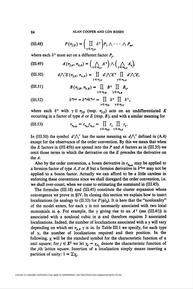
24 ALAN COOPER AND LON ROSEN
011.48) P0>,p) = ( II 3y)p,A--- APffl,
where each 3 Y must act on a different factor PJt
011-49) A(vM,*bJ = ( A aAa{ A Ay),
011-50) dArE(trLE,^E)= IT d'ArEy W d'A%
0H-51) B(vf<B,wb¡B)= H By U By,ye»/,« y^n.B
(111.52) a^s=3^°3^s= II 3Y II 3Y,
where each 3Y with y G 7iy0 (resp. ttjS) acts on an «.differentiated K
occurring in a factor of type A or E (resp. 5), and with a similar meaning for
011.53) r = r, r„ = II r, II r_.
In (111.50) the symbol d'Ar has the same meaning as dAr defined in (A.4)
except for the observance of the order convention. By this we mean that when
the E factors in (IH.45b) are spread into the P and A factors as in (111.35) we
omit those terms in which the derivative on the E precedes the derivative on
the A.
Also by the order convention, a bosen derivative in rv may be applied to
a fermion factor of type A,Eox B but a fermion derivative in d"'0* may not be
applied to a boson factor. Actually we can afford to be a little careless in
enforcing these conventions since we shall disregard the order convention, i.e.
we shall over-count, when we come to estimating the summand in (111.45).
The formulas (III. 18) and (111.45) constitute the cluster expansion whose
convergence we prove in §IV. In closing this section we explain how to insert
localizations (in analogy to (11.33) for P^)^. It is here that the "nonlocality"
of the model enters, for each y is not necessarily associated with two local
monomials in <f>. For example, the y giving rise to an Ay (see (111.41)) is
associated with a nonlocal cubic in <i> and therefore requires 3 associated
localizations. Indeed, the number of localizations associated with a y will vary
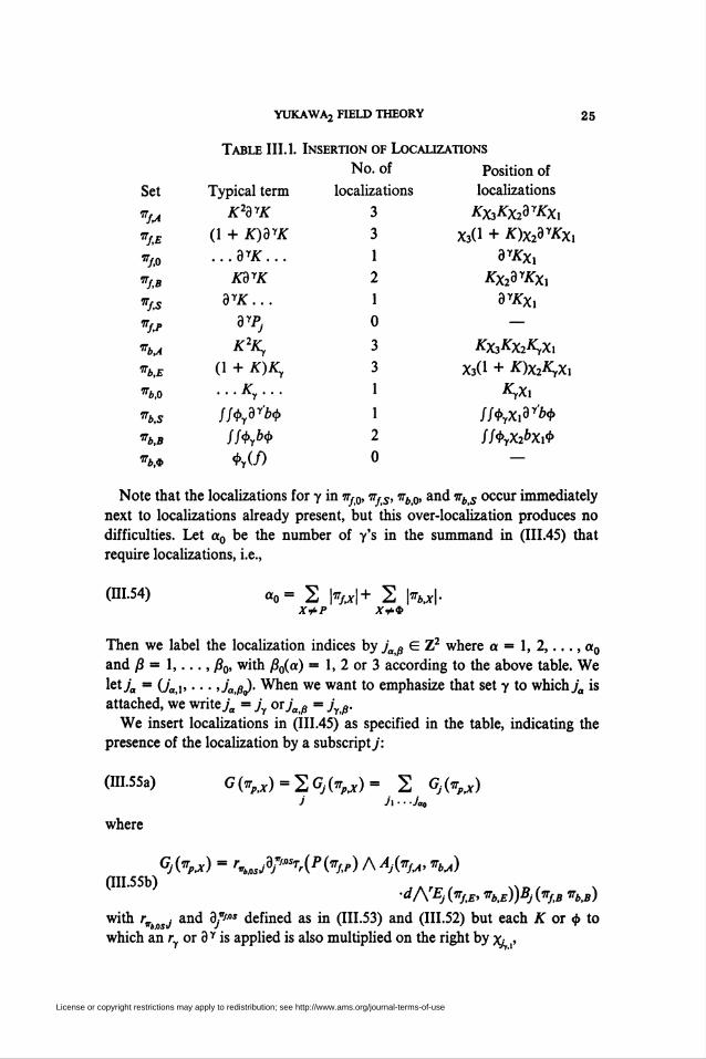
depending on which set irpX y is in. In Table III.l we specify, for each type
of y, the number of localizations required and their position. In the
following, x will be the standard symbol for the characteristic function of a
unit square; for / E Z2 we let x, = Xa denote the characteristic function of
the y'th lattice square. Insertion of a localization simply means inserting a
partition of unity: 1 = Sx^.
License or copyright restrictions may apply to redistribution; see http://www.ams.org/journal-terms-of-use
YUKAWA2 FIELD THEORY 25
Table III. 1. Insertion of Localizations
Set
«JA
mJ,E
"jfl
mJ,s
%'f.P
IT,byA
%b.E
^bfi
'"b.S
'"b.B
%b,<S>
Typical term
K2dyK
(1 + K)dyK
...dyK...
KdyK
dyK...
dyPj
K%
(1 + K)K,...Ky...
//</,?3Y'H
<t>y(f)
No. of
localizations
3
3
1
2
1
0
3
3
1
1
2
0
Position of
localizations
Kx3KX2dyKxl
Xj(l + K)X2dyKXi
3y*Xi
#X23Y*Xi
3^X,
^XA^yXlX3(l + ^)X2^yXi
*yXi
//<r\X26Xl<f>
Note that the localizations for y in wj¡0, wfs, itb0, and trb s occur immediately
next to localizations already present, but this over-localization produces no
difficulties. Let a0 be the number of y's in the summand in (111.45) that
require localizations, i.e.,
(111.54) «o=2 M+ 2 K*lX*P A>*
Then we label the localization indices by jaß E Z2 where a — 1, 2,..., a0
and ß = 1,..., ß0, with ß0(a) = 1, 2 or 3 according to the above table. We
let/, = (/,,,... ,jatß). When we want to emphasize that set y to which/, is
attached, we write/, - jy orjaß = jyB.
We insert localizations in (111.45) as specified in the table, indicating the
presence of the localization by a subscript/:
j j\ • ■ Jaa
(III.55a)
where
(III.55b)•dA'Ej (ttj,E, irbtE))Bj (vJJt vbtB)
with rVbosJ and 3/'os defined as in (111.53) and (111.52) but each K or <f> to
which an ry or 3 Y is applied is also multiplied on the right by x,,»
Gj(vp,x) = \0j;'°%{P(vf<P)AAj(irM, *rM)
License or copyright restrictions may apply to redistribution; see http://www.ams.org/journal-terms-of-use
26 ALAN COOPER AND LON ROSEN
M'J*> *m) = (A KXjiKXjyadyK^)* fyA
and so on.
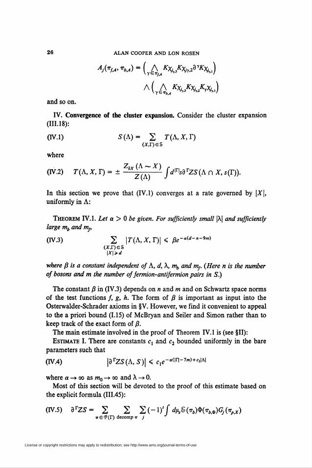
IV. Convergence of the cluster expansion. Consider the cluster expansion
(III. 18):
(IV.l) S(A)= 2 TiA,X,T)(*,r)eS
where
Zav (A ~' X) r(IV.2) r(A, jf, r) = ± Z{K) fdlTlsdTzs(a n x, s(T)).
In this section we prove that (IV.l) converges at a rate governed by |.Y|,
uniformly in A:
Theorem IV.l. Let a > 0 be given. For sufficiently small \X\ and sufficiently
large mb and m¡,
(TW3) 2 \T(A,X, T)\ < ^-«W-»-*»)(A-,r)eS
\X\>d
where ß is a constant independent oj A, d, X, mb and mf. (Here n is the number
oj bosons and m the number of fermion-antifermion pairs in S.)
The constant ß in (IV.3) depends on n and m and on Schwartz space norms
of the test functions /, g, h. The form of ß is important as input into the
Osterwalder-Schrader axioms in §V. However, we find it convenient to appeal
to the a priori bound (1.15) of McBryan and Seiler and Simon rather than to
keep track of the exact form of /?.
The main estimate involved in the proof of Theorem IV.l is (see §11):
Estimate I. There are constants cx and c2 bounded uniformly in the bare
parameters such that
(IV.4) \dTZS(A,S)\ < q(?-«(ir|-7*)+c2|A|
where a -» oo as m0 -» oo and X -» 0.
Most of this section will be devoted to the proof of this estimate based on
the explicit formula (111.45):
(IV.5) 3rZS= 2 2 K-V'f dpßivb)$ivbi9)GjivpiX)weíPír) decompir j
License or copyright restrictions may apply to redistribution; see http://www.ams.org/journal-terms-of-use
YUKAWA2 FIELD THEORY 27
where the localized G, is defined in (111.55). The logic of the proof is exactly
as in the case of P(4>)2 (see the end of §11). First we interchange the sum over
localizations with the sum over partitions (Lemma IV.2). We next count the
number of terms in the summand in (IV.5) in terms of A/(A)'s (Lemma IV.3).
We estimate g-space integrals in Lemmas IV.4, IV.6, IV.7 and Theorem
VII. 14, in such a way as to extract Gx and G2 factors (see §11). These factors
are then used to control Bx and B2.
Before embarking on this project we remark on notation to be used. In
addition to the sharp localizations Xj introduced in §111 we shall also require
smooth localizing functions ^ S C0°° with the properties:
(IV.6) ¡j = 1 on A,: supp Sj C {x\dist(x, A,) < ±}.
In the following estimates we use the letter c to denote various (not neces-
sarily equal) positive constants which may depend on n, m, J, g, h,... but
which are independent of s, A, T and the bare parameters. Similarly we use
the letters 8 and a to denote various universal positive constants where the
constants 8 will always satisfy 5 < 1.
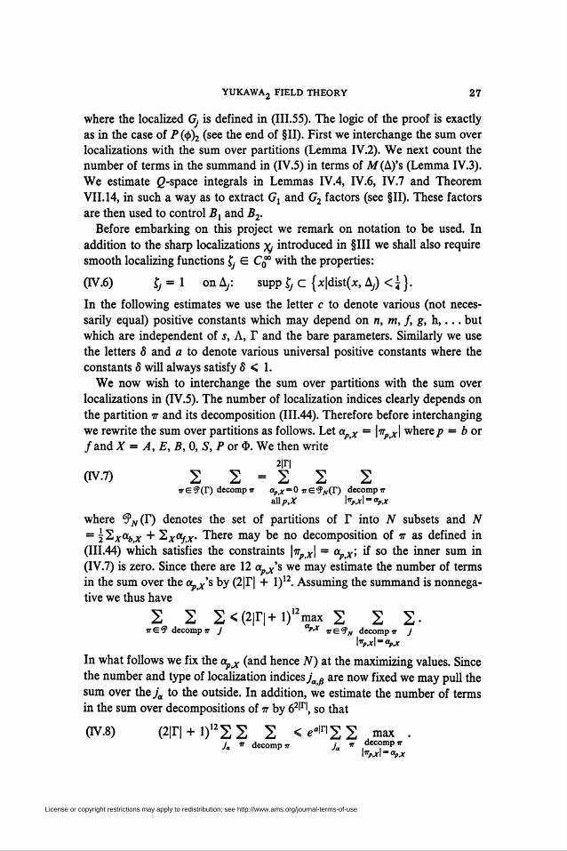
We now wish to interchange the sum over partitions with the sum over
localizations in (IV.5). The number of localization indices clearly depends on
the partition tt and its decomposition (III.44). Therefore before interchanging
we rewrite the sum over partitions as follows. Let apX = \irPtX\ where p = box
j and X = A, E,B, 0, S, P or 0. We then write
api(TV.?) 2 2=222
7reiP(r) decompw <*pj(=0 irS^N(r) decompira&p,X ^pjA-Opjc
where 9N(T) denotes the set of partitions of T into N subsets and N
= 2^xab,x + ^xaj,x' There may be no decomposition of it as defined in
(III.44) which satisfies the constraints \ttp<x\ = apX; if so the inner sum in
(IV.7) is zero. Since there are 12 apX's we may estimate the number of terms
in the sum over the o^'s by (2|T| + l)12. Assuming the summand is nonnega-
tive we thus have
2 2 2<(2|r|+i)12max 2 2 2-in=& decompir j ** isî, decompir j
\*pjc\ = <*PtX
In what follows we fix the apX (and hence N) at the maximizing values. Since
the number and type of localization indices jaß axe now fixed we may pull the
sum over theya to the outside. In addition, we estimate the number of terms
in the sum over decompositions of it by 62'rl, so that
0V.8) (2|T| + 1),22 2 2 <ea|r|2 2 max .ja ir decompir Ja it decompir
License or copyright restrictions may apply to redistribution; see http://www.ams.org/journal-terms-of-use
28 ALAN COOPER AND LON ROSEN
Again to save writing we shall not write in the symbol "max" in (IV.8), but
shall assume that for each/ = (/,) and m E ^(r) we take the decomposition
of tt which yields the maximum in (IV.8). From (IV.5) we thus obtain
Lemma IV.2. For the maximizing values of apJC and ttp^,
(IV.9) |3rZS(i)| < eo|r|2 2 /¿«^fo)*(»w)Wj vestry
where Gj(tt) is defined in (111.55).
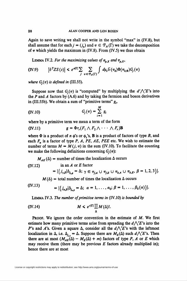
Suppose now that G^ir) is "computed" by multiplying the d'ArE's into
the P and A factors by (A.6) and by taking the fermion and boson derivatives
in (III.55b). We obtain a sum of "primitive terms" g¡,
M
Ov.io) Gj(it) = 2 gt/-i
where by a primitive term we mean a term of the form
0V.11) g = *t,(F, A F2 A • • • A Fr)B
where $ is a product of n <f>'s or <f>y's, B is a product of factors of type B, and
each Fa is a factor of type P, A, PE, AE, PEE etc. We wish to estimate the
number of terms M = M(j, it) in the sum (IV. 10). To facilitate the counting
we make the following definitions concerning Gj(ir):
MAE (A) = number of times the localization A occurs
(IV.12) in an A or E factor
= \{Jyji\\, = A; y e tru U ir}tE u »M u -nb<E, ß - 1,2,3}|.
M (A) = total number of times the localization A occurs
(IV-13) = \{Ja,ß\h, - A; a - 1,.... «o; j8 - 1,..., ß0(a)}\.
Lemma IV.3. The number of primitive terms in (IV. 10) is bounded by
(IV.14) M < eclrIIlM(A)!.A
Proof. We ignore the order convention in the estimate of M. We first
estimate how many primitive terms arise from spreading the d/S^E's into the
P's and A's. Given a square A, consider all the dA'E's with the leftmost
localization in A, i.e. A,- 3 = A. Suppose there are ME(k) such d/S^E's. Then
there are at most (MAE(&) — ME(A) + m) factors of type P, A or E which
may receive them (there may be previous E factors already multiplied in);
hence there are at most
License or copyright restrictions may apply to redistribution; see http://www.ams.org/journal-terms-of-use
YUKAWA2 FIELD THEORY 29
(MAE(A) - ME(A) + m)\<2M^(A)-^(A)+mA/£(A)!
(MAE(A)-2ME(A) + m)\
ways of distributing these E's. Thus we conclude that all together there are at
most
(IV.15) II 2mà)+mME(A)\A
M£(A)>0
primitive terms arising from multiplying in the E's.
Next, let Md(A) be the number of derivatives in 3/'°* and r j localized in
A. Since there are at most (M (A) - Md(A)) places for them to be applied, we
estimate the number of ways of applying these derivatives as in (IV.15) by
0V.16) II 2MWMd (A)!.A
Md(h)>Q
The derivatives in the $ and P factors (111.47) and (111.48) contribute a
factor to M but this factor is bounded by n\m\. Hence from (IV.15) and
(IV. 16) we conclude that
A/< cmtíME(A)\Md(A)\
Now
AA/(A)>0
ME(A)\Md(A)l< (ME(A) + Md(A))\< M(A)\,
and since each y has at most 6 associated localizations,
(IV.17) 2^(A) < 6|T|.A
The last three inequalities yield the lemma. □
The next step in estimating the summand in (IV.9) is to represent the
expectation &(irb), as defined in (111.38) and (111.40), by positive Gaussian
measures. There is one simple case in which there is no need for this step or
even for &y; namely, if for some decomposition of it we have both oc-
currences of some y in irb<s>, then we obtain a factor (h¡, yyCh¡) which can be
estimated by
(IV.18) \(hit dyChj)\ < cK6(y)m¿s>M
by (11.30). It is to be understood in the sequel that we always apply the
estimate (IV.18) and do not introduce dummy fields for such a y.
Now, although dyC(x,y) is pointwise positive, it is not positive as an
operator except in the case |y| = 1. Thus there will not, in general, be a
corresponding positive measure. However we can write 3YC as a linear
License or copyright restrictions may apply to redistribution; see http://www.ams.org/journal-terms-of-use
30 ALAN COOPER AND LON ROSEN
combination of suitable positive operators. We do so in two ways depending
on whether we wish to exhibit the G, or G2 decay (see §11). For G2 we note
that if b is, say, the first bond in y, then by (VI. 19),
(IV.19a) dyC(s)=d"dy~"C(s)= 2 (-l)lyH"MCy>,(L.)PCy~b
where
(IV. 19b) Cy»=3*C(S)| s ~ 1 on ps = 0on y~(i>u¿)
Since only a single bond derivative is involved in (IV. 19b), dbC(s) = 8bC(s)
is positive definite (see e.g. [12]). In other words, (IV. 19) represents 3YC as a
linear combination of 2IyI_1 positive definite operators, each of which is
continuous on S(R2) and each of which has appropriate G2 decay: as we
prove in Corollary VI .2, for any e < |,
0V.2O) \\t>%CyJkD°\\L2{R4) < c(e)mge-Sm°Wy'»+d(y'k)X-
where the constant c(e) is independent of /, y, v, k, where
D = (-A + m2f2,
and where (b is the first bond in y)
(IV.21) d(y, i) = dist(6, A,).
Let d[Hy „ be the Gaussian measure on a copy Qy of § '(R2) with covariance
0V.19b), and define
(IV.22) dli2(-nb)= ® dii,^ on Q(7tb)= X Qyyew,, y£wl
where v(y) is some subset of y ~ b. Then we can represent the expectation
S(iTb) in (IV.5) as a linear combination of T[ySv2M~x = t?°(|r|) integrals of
the form ¡Qt„) dfcfa) with ̂ >y the coordinate function on Qy.
For the G. decay we restrict our attention to "large" y's. By definition a
large y is one for which |/a(y)| > 1 for all permutations a (see (11.29) for the
definition of |/„(y)|). It is easy to see that
(IV.23) |y| > 7 implies y is large,
and that if y is large then for all permutations a,
(IV.24) |/0(y)| >|y|/14.
If y is not large we say it is small. The point of these definitions is that for
small y, K6(y) > 1 (see (11.31)) and so there is no (?■ decay; whereas for large
y there is G, decay and, moreover, we can extract a convergence factor.
Explicitly, let
(1V.25) G1(y,S) = 2<?-iw°l''(Y)|.
License or copyright restrictions may apply to redistribution; see http://www.ams.org/journal-terms-of-use
YUKAWA2 FIELD THEORY 31
Then
(IV.26) K6 (y)s < Gx (y, 5/3) < e-*«**^ (y,82 )
where 5/3 - 145! + 52 with 5,. > 0 (we have used (IV.24)).
For the Gx decay for large y we appeal to Lemma VI. 11 which asserts that
3 yC may be written as a difference,
(IV.27) 3*C = Cr>+ -CY(_,
where Cy± > 0 axe not necessarily the positive and negative parts of 3YC, but
for anyp < oo can be chosen to satisfy
(IV.28) \\Cy¡±\\L,<cMmSGx(y,8)
where 5 > 0,ÇX and f2 are any two localizations as defined in (IV.6), c(p) is a
constant independent of y, £,, f2, and Gx is defined in (IV.25). Moreover, for
any e < 1, there is a constant c(e) < oo such that
0V.29) ||Z>eCy>±Z)e||L2< cM<<7, (y, 5).
As in the G2 case, we introduce Gaussian measures dpy± on Qy with
covariance Cy>± for each large y. For the small y's we use a G2 measure. Then
we can write the expectation jdpc,s/b(irb) as a linear combination of e°(lr|)
integrals of the form JQ^b)dpx(tTb) where
dPl(n)= ® ¿/iy,± ® ̂ (y),ye.irt yevf
where itb (resp. nbs) axe the large (resp. small) y's in itb. When we insert dpx or
dp2 into (IV.9) it is to be understood that the y's and ± signs are fixed to
maximize the integral and that the e°(lrl) bound on the number of terms in
the sum over v and ± has been absorbed into the e"^. Thus from (IV.9) we
have
0V.30) 13TZS(s)\ < e°N2 2 min f dpc(s)® dpfiAit)J weiPw(r)''=1'2 JQxQ(«b)
We are now ready to estimate the contribution to (IV.30) of each primitive
term in (IV. 10), i.e. to estimate an expression of the form
(IV.31) mini
j dpc,s) ® dp^rr(Fx A • • • A Fr)B
From definition (111.32) we find by the "weak linear lower bound" of
Theorem VII. 14' that for any p < oo and q > p there is a constant c
independent of m0, r and A such that
(IV.32) ||rr(F, A • ' • A Fr)\\LP< e^HllIllFJlJIl a Wl"
where || • H, denotes the trace norm on %. By Holder's inequality we then
License or copyright restrictions may apply to redistribution; see http://www.ams.org/journal-terms-of-use
32 ALAN COOPER AND LON ROSEN
bound (IV.31) by
(1V.33) e^+l^min 11*11n̂ BF.B,a-l
\\B\\l?If
where Lf denotes the norm in L4(Q X Q(ttb), dnc,s) ® tfju,).
The last three factors in (IV.33) are estimated in Lemmas IV.4, IV.6, IV.7
below. We shall always estimate the minimum over i in (IV.33) by the
geometric mean.
Lemma IV.4.2
(IV.34) H llallí2 < c II <G,(y,S)i'=l ïEirM
where the factor mj¡ can be replaced by m0-5l'Y'/2 if y occurs twice in 7ri<t.
Proof. If y occurs twice in 7ri4, we simply extract the factor (IV. 18)
without introducing dummy fields <by into $ or measures d^, or d¡iY±.
Otherwise, the evaluation of \\$\\i* is a standard calculation involving (IV.20)
and (IV.29). The constant c in (IV.34) depends on n and Schwartz norms of
the form ||Z) "T.,.||¿2. Q
Consider next the second factor (involving F„'s) in OV-33). In order to
understand the choices we make in estimating the F„'s, the reader should bear
in mind these facts: K is in any Gpj!., (defined in (III. 12)) with/? > 2; dyK isin any Qp¡p;, withp > \ ; we can improve the Qpj)., property of K, in the sense
of decreasingp, by applying operators D ~' with e > 0; operators D' worsen
Qpj)., properties. Precise statements of the above may be found in §VIL2.
Consider now a typical factor Fa occurring in (IV.33); e.g.,
(IV.35) Fa = AE = [K^K^KXiJlxjJl + K)XjJYKXjJ
where, of course, jyX = fy.3. We insert smooth localizations Ç, by Xj = XjHj t°
obtain
r. = (%)(Ä)(y%) • • • (Wyj&Ü-We indicate schematically (i.e. without writing in the localizations) the
manner in which we estimate H^JI.. First,
i^-36) F<«lli<HII,FII-Then, using Holder's inequality on the ||yi||i factor we get <24 and ßj norms
on the K and 3 yK factors (resp.), i.e.,
(iv.37) mx<\mmvxyWe estimate the factors K and dyKin E by operator norms and then by Q4
License or copyright restrictions may apply to redistribution; see http://www.ams.org/journal-terms-of-use
YUKAWA, FIELD THEORY 33
and ßj norms (resp.):
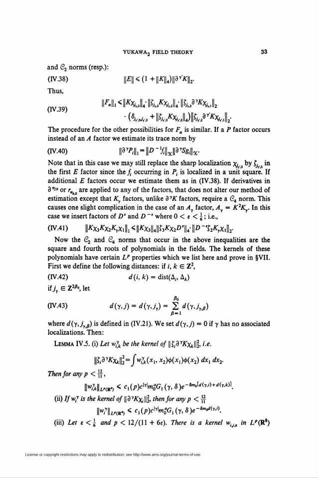
(IV.38) \\E\\<(l+\\K\\4)\\ay'K\\r
Thus,
(IV 39) "Fa111 < ¡^A'lhMX' H^9^'112
■(^HkMMkr'K%J2The procedure for the other possibilities for Fa is similar. If a P factor occurs
instead of an A factor we estimate its trace norm by
(IV.40) \\3yPi\\l = \\D-xJi\\%\\dySgi\\%.
Note that in this case we may still replace the sharp localization jg by f, in
the first E factor since the / occurring in P¡ is localized in a unit square. If
additional E factors occur we estimate them as in (IV.38). If derivatives in
3"/.o or r are applied to any of the factors, that does not alter our method of
estimation except that Ky factors, unlike 3 yK factors, require a 64 norm. This
causes one slight complication in the case of an Ay factor, Ay — K2Ky. In this
case we insert factors of De and D _e where 0 < e < | ; i.e.,
(IV.41) ||A-x3A'x2A;x,||1<||A'x3||4||Í3A'X20e||4-||o-Í2A'yXi||2.
Now the C2 and ß4 norms that occur in the above inequalities are the
square and fourth roots of polynomials in the fields. The kernels of these
polynomials have certain Lp properties which we list here and prove in §VII.
First we define the following distances: if /', k E Z2,
(IV.42) d(i, k) = dist(A(., Ak)
iijy E Z2B°, let
A>(IV.43) d(y,j) = d(y,jy) - 2 d(y,jy,B)
ß=\
where d(y,jyB) is defined in (IV.21). We set d(y,j) = 0 if y has no associated
localizations. Then:
Lemma IV.5. (i) Let wyk be the kernel of WWKyjfc, i.e.
||£i9Y*&¡2"/w/M*i' *2>K*i)t>(*2) dxx dx2.
Then for any p < j2-,
IM/AR«) < cx(p)cMmSGx(y,8)e-s^M^(y,k)\
(ii) IJw? is the kernel oj \\dyKXi\\% thenjor any p < $
IKIIx/Ort < cx(p)c\y\ma0Gx(y,8)e-Sm^y'i\
(iii) Let e < I and p < 12/(11 + 6e). There is a kernel wiJe in LP(RS)
License or copyright restrictions may apply to redistribution; see http://www.ams.org/journal-terms-of-use
34 ALAN COOPER AND LON ROSEN
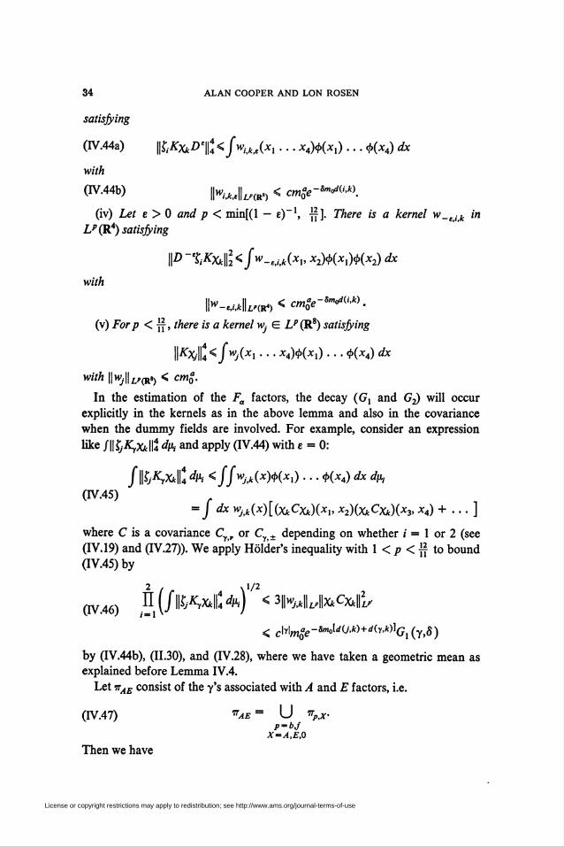
satisfying
(IV.44a) ftA*J>TÍ </>W*, . . . x4)4>(Xl) .. . <p(x4) dx
with
(IV.44b) IKUUr«) < cmSe-WOM
(iv) Let e > 0 and p < min[(l — e)_1, -Jy]. There is a kernel w_elk in
Z/(R4) satisfying
P't,ÄÄE</w-*a(*i. *2)<H*.)</>(*2) dx
with
\\W-^\\L^<C<e~Sm0flU'k)'
(v) Forp < jf-, there is a kernel w¡ E LP(RS) satisfying
||^xJ4</w,.(x, . . . *4)<i>(*i) . . . <b(x4) dx
with WwjWuqP) < cm%.
In the estimation of the Fa factors, the decay (G, and G^ will occur
explicitly in the kernels as in the above lemma and also in the covariance
when the dummy fields are involved. For example, consider an expression
like iUjf^XkWt dii¡ and apply 0V.44) with e = 0:
jïl?Ax*||4 fa <ffwjAx)<s>(xi) ■ ■ • <K*4) dx dp,(IV.45)
= J dX rt^jOLGCfcCXftX*!, *2)(X*Cxjfc)(*3. x4)+ ... \
where C is a covariance Cyv or Cy± depending on whether / = 1 or 2 (see
(IV. 19) and (IV.27)). We apply Holder's inequality with 1 < p < jf to bound(IV.45) by
2 / r \X/2
(IV.46) n(/ll^x,|i:%) < HMiMCxù
< clYlw,0^-W</O,«+rf(Y,*)](;i (Y)S)
by (IV.44b), (11.30), and (IV.28), where we have taken a geometric mean asexplained before Lemma IV.4.
Let wAE consist of the y's associated with A and E factors, i.e.
(IV.47) *ae = U v,jrP = bj
X=A,E,0
Then we have
License or copyright restrictions may apply to redistribution; see http://www.ams.org/journal-terms-of-use
YUKAWA2 FIELD THEORY 35
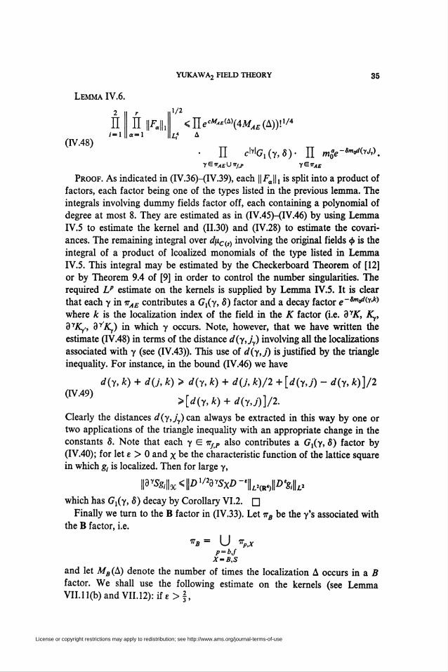
Lemma IV.6.
2 II r m'/2
n(IV.48)
n n^-iiia-l
<JJecAi-(i)(4A^£(A))!1/4
II cWG^y.5). II mZe-WtoJ,,.yeirAEuirfJ, ye-TAE
Proof. As indicated in (IV.36)-(IV.39), each ||.Fa||, is split into a product of
factors, each factor being one of the types listed in the previous lemma. The
integrals involving dummy fields factor off, each containing a polynomial of
degree at most 8. They are estimated as in (IV.45)-(IV.46) by using Lemma
IV.5 to estimate the kernel and (11.30) and (IV.28) to estimate the covari-
ances. The remaining integral over dpc(s) involving the original fields <f> is the
integral of a product of lcoalized monomials of the type listed in Lemma
IV.5. This integral may be estimated by the Checkerboard Theorem of [12]
or by Theorem 9.4 of [9] in order to control the number singularities. The
required LP estimate on the kernels is supplied by Lemma IV.5. It is clear
that each y in irAE contributes a Gx(y, 8) factor and a decay factor e~Smcdiy'k)
where k is the localization index of the field in the K factor (i.e. dyK, K^,
3^., dyK/) in which y occurs. Note, however, that we have written the
estimate (IV.48) in terms of the distance d(y,jy) involving all the localizations
associated with y (see (IV.43)). This use of d(y,j) is justified by the triangle
inequality. For instance, in the bound (IV.46) we have
d(y, k) + d(j, k) > d(y, k) + d(j, k)/2 + [diy,j) - d(y, k)]/2
0V.49) , , ,>[d(y,k) + d(y,j)]/2.
Clearly the distances d(y,jy)can always be extracted in this way by one or
two applications of the triangle inequality with an appropriate change in the
constants 5. Note that each y G itSP also contributes a Gx(y, 8) factor by
(IV.40); for let e > 0 and x be the characteristic function of the lattice square
in which g¡ is localized. Then for large y,
Wsgl\\x<WD^ysxD-'¡íl(fñp%y
which has G,(y, 5) decay by Corollary VI.2. □
Finally we turn to the B factor in (IV.33). Let irB be the y's associated with
the B factor, i.e.
*B - U *pJCP = bj
X=B,S
and let MB(A) denote the number of times the localization A occurs in a B
factor. We shall use the following estimate on the kernels (see Lemma
VII.ll(b)andVII.12):ife>|,
License or copyright restrictions may apply to redistribution; see http://www.ams.org/journal-terms-of-use
36 ALAN COOPER AND LON ROSEN
2
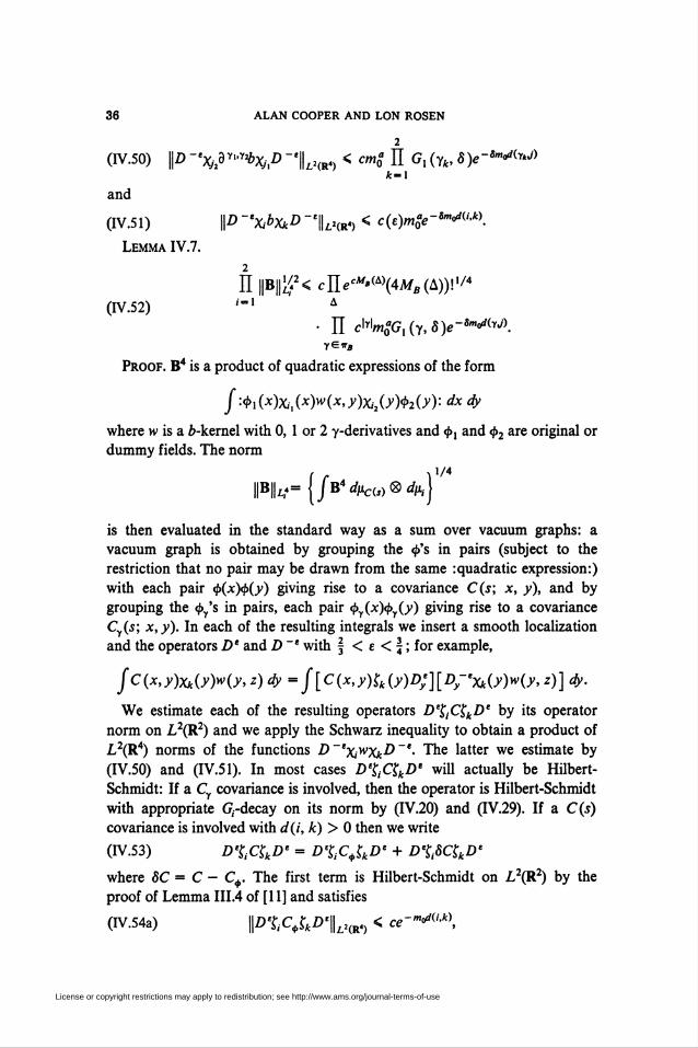
(IV.50) \\D-%dy^XjP"IUr«) < cmS II G,(yk, 5)e-*»rf<»J>k~\
and
(IV.51) IP -'XtbxtD -E||LI(R4) < c(e)mSe-Wk\
Lemma IV.7.
n||B||if<cne^(A)(4MB(A))!'/4
(IV.52) ,=1 A• II clYlm0aG,(y,S)e-Smorf(Y-/).
Proof. B4 is a product of quadratic expressions of the form
f :'}>i(x)Xil(x)w(x,y)xil(y)<b2(y): dx dy
where w is a ¿-kernel with 0, 1 or 2 y-derivatives and <f>¡ and <i>2 are original or
dummy fields. The norm
||B||A«- {/b4^)®^.}
is then evaluated in the standard way as a sum over vacuum graphs: a
vacuum graph is obtained by grouping the </>'s in pairs (subject to the
restriction that no pair may be drawn from the same : quadratic expression:)
with each pair 4>(x)<b(y) giving rise to a covariance C(s; x, y), and by
grouping the <|>y's in pairs, each pair <by(x)<by(y) giving rise to a covariance
Cy(s; x,y). In each of the resulting integrals we insert a smooth localization
and the operators De and D ~' with § < e < f ; for example,
Jc(x,y)Xk(y)w(y,z)dy = f[C(x,y)tk(y)D;][Dy-'xk(y)w(y,z)] dy.
We estimate each of the resulting operators D%¡C$kD' by its operator
norm on L2(R2) and we apply the Schwarz inequality to obtain a product of
L2(R4) norms of the functions D~txiwxkD~t. The latter we estimate by
(IV.50) and (IV.51). In most cases D%CÇkD' will actually be Hilbert-
Schmidt: If a Cy covariance is involved, then the operator is Hilbert-Schmidt
with appropriate G,-decay on its norm by (IV.20) and (IV.29). If a C(s)
covariance is involved with d(i, k) > 0 then we write
(IV.53) D%C$kD' = D%C¿kD' + D%8C$kD'
where 8C = C - Cr The first term is Hilbert-Schmidt on L2(R2) by the
proof of Lemma III.4 of [11] and satisfies
(IV.54a) \\E>%C^kDe\\LHRt) < ce~m^k\
License or copyright restrictions may apply to redistribution; see http://www.ams.org/journal-terms-of-use
YUKAWA2 FIELD THEORY 37
while the second term is Hilbert-Schmidt by Lemma VI. 10 and satisfies
(IV.54b) \]D%8<Xk*>'L*aft < cmSe-Sm^k\
If in (IV.53) d(i, k) = 0, then the second term on the right still satisfies
(IV.54b) while the first term is evidently a bounded operator (to see this,
simply omit the f's). We conclude that D%CÇkD* is always a bounded
operator with d(i, k) decay as in (IV.54). This decay is important for
controlling the number singularities, i.e. the sum over vacuum graphs: using
(IV.54b) and Theorem 9.4 of [9] we obtain the estimate ]lAecAM^\4MB(A))\
for this sum. (We do not require such an argument for the <by pairings since
each field <by can occur at most 8 times in B4.)
Collecting all of these estimates, we obtain (IV.52). Note that an applica-
tion of the triangle inequality may be required again, just as in (IV.46); e.g. to
convert the d(jy,iJy,d and d(y,jyA) decays of /<px, bx¡ fa to a d(y,jy) decay.
DWe now collect the above estimates to obtain the desired bound on (IV.31).
The numerical factors in (IV.48) and (IV.52) may be simplified somewhat by
[(4MAE (A))! (4MB (A))! ]1/4 < 4""<*>MAE (A)\4M'™MB (A)!
< 4W(A)A/(A)!.
By (IV.33), (IV.34), (IV.35), (IV.48) and (IV.52) we thus bound (IV.31) by
c exp clr + |A| + |T| + 2 AT (A)) IIM (A)!(IV.55) L a J a
• II «0-,M II «Í II Gx(y,8)e-Sm^y^yGvb.M yew yen-lu^
where the set ttb^2 consists of those y's which occur twice in trb$ (see Lemma
IV.4) and the set it' = itb U irf\(irb¿, U irftP). Note that the factor m¡¡ in
(IV.34), associated with those y's applied once to $, has been absorbed into
the mjj associated with the other occurrence of y in 77'. We can simplify
OV.55) somewhat by (IV. 17) and the estimate r < m + 2\T\ (see (111.46));
also we identify the two occurrences of a y in irb so that it\ u tt¡ may be
replaced by m, ttb^2 replaced by 77,1, consisting of y's exclusively associated
with Í», and tt' redefined to consist of those y's in 7r which are not associated
exclusively with a?or$ factor. Note that a y G 77 may now have as many as
six localizations/y ß. Using Lemmas IV.2 and IV.3 we then obtain
Corollary IV.8.
License or copyright restrictions may apply to redistribution; see http://www.ams.org/journal-terms-of-use
38 ALAN COOPER AND LON ROSEN
\ZTZS(s)\ < ec<lrMAl>2 2 IlM(A)!2J ire9N(T) A
(IV*56) • II nÇ™ II mS II Gl(y,8)e-Sm^\ySiTQ y^ir' y Sir
We are left with the same expression as in the P(<b)2 case except for two
differences:
(i) the number of localizations / ß associated with y varies from 1 to 6,
instead of being exactly 2;
(ii) there is a large factor m^ instead of the convergence factor /Wr7a'r'.
Difference (i) is minor, for we still have the relation (11.34) and, conse-
quently, the bound, for 0 < e < \,
(IV.57) IlA/(A)!2<exp c^M(A)x+t < ec^exp\c^d(y,jy)lA L A J L J
Thus for sufficiently large m0 we can absorb the factor n¿M(A)!2 into the G2
decay factor, i.e. G2 controls B2.
As for (ii), we now liberate the coupling constant X so that each K factor
acquires an associated X and each B an associated X2. It is then easy to see
that with each y E it' we may associate at least a factor of |A|'/2. If we choose
X so that
(rv.58) /<IAI1/4 < 1
we deduce from (IV.56) and (IV.57) that for sufficiently large m0,
|3rZS(i)|< ec(lrl+lAl>2 2 II m0-5lYl
J * yGij
0V.59) „ , „ „• II \X\x/4IÍGl(y,8)e-s'"^yA
y £ it' y e it
It should now be clear how we extract the convergence factor. For large y's
in it we can extract a factor e~Sm<>M from G,(y, 8) by (IV.26). For small y's in
Tr<t, and it' we have convergence factors /w¿"5|yl and |X|IyI/28, respectively; here
we have used the fact (IV.23) that a small y satisfies |y| < 7. The only
remaining y's are small y's associated with P factors. But there can be at most
m such y's each with at most 7 bonds. We conclude that for any a > 0, if we
choose m0 sufficiently large and |X| sufficiently small so that m¡¡, \X\X/2S,
e~Sm« < e~", then we have
|3rZLS(i)| < e^M^-^ri-7"1). 2 2 II G, (y, fi)*-**«*».j wS^jv yen
We now rejoin the P(<|>)2 proof: we pull out the factor
max„6g, Uye„e~Bm'^(y'^, sum over m to get a factor e°(lrl> by Lemma II.2 (i.e.
Gi controls 5,), and then sum over each jaß to get another factor e0(^\
License or copyright restrictions may apply to redistribution; see http://www.ams.org/journal-terms-of-use
YUKAWA, FIELD THEORY 39
Therefore
|3rZS(s)| < ce-<*—m--»**4N
which is Estimate I (i.e. estimate (IV.4)). The proof of Theorem IV.l now
follows easily:
Proof of Theorem IV.l. It remains to check Estimate II (see (11.22)). We
use a dominated convergence type argument, namely Lemma 3.5 of [25]: if
p3A(\) denotes the renormalized determinant with A = A and s = 0 on 3A,
then we know (see §VII.4) that, for any p < oo, \\paA(X)\\ Lndl¡C(j < oo, uni-
formly for X in a bounded interval. Since p3A(A) -» 1 pointwise and dpC{s) is a
probability measure, we conclude that p3A(a)-»1 in Lx(dpC(s^ as A-»0.
Hence for sufficiently small |X|, Z3A(A) = JpdA(X) dpC{s) satisfies {■ < |Z3A(A)|
< 2. (Presumably, p(s) and Z(s) axe nonnegative as in the s = 1 case [22], but
we do not have a proof of this.) As in [9] we conclude that by Estimates I—III,
2 \T(A,X,T)\<c 2 e-«(lrl-7m)+cl*L(A-.neS \x\>d
\X\>d
But by the definition of §, every component of X ~ Tc meets X0 so that
\T\>\X\-\X0\>\X\-n - 2m.
The theorem follows from the last two inequalities. □
V. Consequences. In this section we shall establish the major consequences
of the convergence of the cluster expansion (in particular, Theorem LI). Our
proofs are brief since, once the appropriate doubling procedure is introduced,
the Y2 proofs follow those of P(<i>)2. Our first result is
Theorem VI (Cluster Property). Let a > 0 be given. Suppose that
Ía = Ua,¡)> Sa - (Sa,¡) a"d hA = (hA¡) are Schwartz space test Junctions with
support in the region A c R2, and similarly JB, gB, hB have support in the region
B. Let J= (JA,jB), g = (gA, gB), h - (hA, hB). Then Jor any given X we can
choose mb and m} sufficiently large so that
(v.i) \SA (f, g, h) - SA (fA, gA, hA)SA (fB, gB, hB)\ < /fe-"(«U*)-<>
where ß = ß(f, g, h) is independent of A and depends on f, g, h only through
appropriate (translation invariant) Schwartz space norms, the constant c depends
only on the order ofSA, and d(A, B)is the distance between A and B.
Proof. We shall assume that the number mA of/< ,'s equals the number of
gA ,'s (and similarly for B). If not, then the subtracted term in (V.I) vanishes
and we simply apply the cluster expansion to SA(J, g, h) without the necessity
of a doubling procedure. We remark that it is possible to compare directly the
cluster expansions for the Schwinger functions on the left side of (V.I)
License or copyright restrictions may apply to redistribution; see http://www.ams.org/journal-terms-of-use
40 ALAN COOPER AND LON ROSEN
provided we also multiply SA(f, g, h) by 1 = SA(l) and perform a cluster
expansion for it as well. However, as in [9], it is simpler to "double" the
theory as follows:
(i) (Boson doubling). We let (g(0, <#>w, dpï*) for / = 1, 2 be two identical
copies of the free boson field on Q(/) = S '(R2). Define a new process by the
independent sum t> = <f>(1) + <>(2) on Q = Qw X g(2) with measure dß =
dpw X 4i(2). We may introduce 5 B.C. for 4> by dp¿(s) = <//ic¿) x fací) ™ta
C(s) = C(s) © C(s) on S = S(R2) © S(R2).
(ii) (Fermion doubling). We let Sí?0, i = 1, 2, be two identical copies of %
and we define % = %l) © 302). If /"(<!>) is a_ function on S' taking values as
an operator on %, define the operators on %:
(V.2a) /■<»(*) = F(<i»(1)) © 0, /-(2)(^) = 0 © F(>(2))
and
(V.2b) F (*) = F(<¡>(1)) © F(<b{2)) = Fw(4>) + F(2)(¿).
With K given by (III.3), we define
p(4>) - detren(l - /f (*)) = det3(l - K)exp[-{- :Tr(K2 + &K):].
The Schwinger functions for the doubled theory are defined as in (III.l 1) in
terms of p, dß, and fm = mlTr^^. Just as in (111.14)—(111.16) we have the
factorization
(V.3a) p(¿) - p(<í>(,))p(<í>(2))
and so
(V.3b) Z = ]>(*) dß = /pfo™) <V n/p(<f>(2)) d^ = Z\
Suppose we rewrite formula (III.l lb) for (/, g, h) as
SA(f,g,h) = Z-xfTm(AmR-QAAQB)pd¡i
where, for X = A or 5, Qx = $(hx) Ajtfxj with
Pxj = {D~XgXj>-)%SnfXJ,
and where m = mA + mB. Let 0¿° be the operators on Am*3C defined by
"ijr
where O^A*) - n^0^) and Px') is as defined in (V.2a). Then we claim
that
S = z-x ffm(AmR (QAl) - ßS°) A(ßi° - Q?))~p *(V.4) ^
= 2[5A(/, g, A) - SA(fA, gA, hA)SA(fB, gB, hB)\.
License or copyright restrictions may apply to redistribution; see http://www.ams.org/journal-terms-of-use
(V.5)
YUKAWAj HELD THEORY 41
The identity (V.4) follows from the direct sum structure % = 30e0 © 3tf2).
ForAmR(QAl)-QA2y)A(QP-QP)
= AmxwQAl) A QBn + Am*(2)ßi2) A ߣ°
- AmARwQAx) A Am"R(2) • QB2)
- AmAR{2) • ßi2) A Am^(1) • Qbx)-
We apply rm to (V.5), observing that by Lemma A.1 we obtain a factorization
of the off diagonal terms, e.g.,
fm(Am^(1)-ßi0AAm^(2)ßF)
^ - fmA (A"^(1) • ßj°) t. (A"**(2) • QB2)).
Noting that fm((AmÄ(0ß(0)(^))= ^((A^ßX^0)), integrating with re-
spect to p dp, and invoking (V.3) we deduce (V.4).
The left side of (V.4) has the appropriate form for an application of the
cluster expansion, i.e., it has the form (III. 11) and, furthermore, it decouples
at s — 0. For suppose that A and B belong to disjoint components A^ and AB
of R2 ~ T2. Then just as in (V.6) we have by Lemma A.1,
fm[AmR-(QAX)-QB2))A(QBx)-Q(B2))]
CV'7) - *ml W** W - Qa2))] • fmi[ Am'iB (fii» - fi?*)]where 7?^ = (1 - A'AnA )-1. (Here it is the decomposition of the doubled
theory induced by the direct sum decomposition of L2(R2) that is involved.)
The integral of (V.7) now factors by (III. 16). If T fails to connect A and B,
then the corresponding term 3 TZS in the expansion factors as
3rZ5= II dr*ffmx[Am*Rx-(Qxi)-Qx2))]pAxdß
and so vanishes by the 1 <-» 2 symmetry.
Let 2 be the set of values of (X, mb, mj) for which the cluster expansion for
(V.4) converges in the sense of Theorem IV.l (i.e. 2 consists of sufficiently
small X and sufficiently large mb, mf); and let 2' be those (X, mb, m/) for which
(V.4) satisfies the desired bound (V.l). As in [9, Theorem 2.1] we deduce that
2 c 2'. It remains to show that 2' contains points with arbitrary X.
But the Schwinger functions SXm A(j, g, h), where we have denoted the
dependence on the bare parameters by additional subscripts, are invariant
under the change of variables:
A-»rA, mb^rmb, m}-*rmf, A->r-1A,
h(x)^r2h(rx) J(x)-*r3/2J(rx), g(x) ^ r3/2g(rx).
This follows by a simple scaling argument based on the fact that <b(x; mb) and
License or copyright restrictions may apply to redistribution; see http://www.ams.org/journal-terms-of-use
42 ALAN COOPER AND LON ROSEN
<b(r xx; rmb) are isomorphic processes. Consequently, if (X, mb, mj) E 2 with
decay rate e~c""-A,B) then so is (rX, rmb, rmj) with decay rate e-ad(rA<rBy =e-rad'A,B)^ r-i
Remark. The results for large X can also be obtained via a convergent
cluster expansion provided we replace the unit squares with squares of side
length L = d/m0, where, for convenience, we have taken mb = mf= m0 and
where d is a constant to be determined. We sketch this argument: First we
rescale lengths as in the above proof with r = l/m0 to obtain an equivalent
theory with bare parameters X' = X/m0, m'b = mj = m'0 = 1, and interaction
region A' = m0A. We claim that the cluster expansion for this new theory
with lattice spacing L' = r~lL = d converges as in 0^.3) provided L' is
chosen large enough and X' small enough (and hence that the cluster expan-
sion for the original theory with lattice spacing L converges for any X
provided d and m0 are chosen large enough). To see this, consider the bound
which is the analogue of (IV.56):
|3r'ZS(A")| < eclr'l+c^'l2 IlA/(A)!2 II |X'|,/2
(IV.56')• II L'aGl(y,8)e-Sd{yJ\
yGir
Note that the factors G, and e~Sd(yJ) involve distances based on a unit of
length L' and that instead of factors m% there are now occur factors of L'a
since the local W estimates are calculated over squares of side L'. As in
(IV.56), we can extract a convergence factor e~SL'M from G,(y, 8) for large
y's. Next we choose L' sufficiently large for the combinatorial arguments of
the cluster expansion (i.e. G, controls 2„ and e'^^^ controls UAM(A)\2).
We then choose X' sufficiently small to give a convergence factor for the small
y's (except for the at most n + m y's in tt ~ it'), thereby controlling the
factors L'a. The only additional feature is that the crucial estimate |r| > \X\
- n-2m (see the proof of Theorem IV. 1) becomes |F| > \X'\/L'2 - n -
2m. But this presents no problem as the linear lower bound constant c2 in
(IV.56') can be made arbitrarily small by choosing X' small enough. Finally,
for any choice of L, the bound (11.22) on Z3A(A) will hold for all sufficiently
small X'.
We now turn to the existence of the infinite volume limit.
Proof of Theorem 1.1(a). By the scaling argument used in the proof of
Theorem V.l it is sufficient to prove the theorem for values of X and m0 for
which the cluster expansion applies. We consider the effect of increasing the
interaction region A by adding a single lattice square A. To do this we
interpolate between xA and xAua by hT = Xa + tXa and write
License or copyright restrictions may apply to redistribution; see http://www.ams.org/journal-terms-of-use
YUKAWA2 FIELD THEORY 43
where S(r) is defined as in (1.3) with Xa in 0-5) replaced by hT. As in [8,
Theorem 2.2.2] it suffices to bound dS(r)/dr by
(V.8) \dS(T)/dr\< ce-ad^'xo)
where a and c are positive constants (independent of A and A) and X0 is a
fixed set which contains the supports of all the test functions in S.
As in (111.26) and (111.31) we find that
£z(r)- -/[!*«,) + § P dp
and
= f [-Tm+l{Am+lR- P AAT) + Tm(AmR- PdAmET)
-Tm(AmR-P)f}pdp
where
A = Vlfr\2
drAT = K(r)2 §■ = K(r)2KA, ET = (1 + K(r))KA,
4jL = :Tr[ KAKA + r(K2+ K¡KA )]: - :Tr KAKA: + rBA.
Thus we obtain
j-TS(T) = Z-ij-TZS-SZ-xj-TZ=TE-TA-TB
where
T1¡'Z-ijTm(AmR- PdAmET)Pdp,
TA = Z-xfTm+l(Am+XR-PAAT)pdp
-Z-2fTm(AmR-P)pdpfTl(RAT)pdp,
TB = Z~X fTm(AmR-P)fpdp-Z-2fTm(AmR-P)Pdpffpdp.
Consider first the term TE. To obtain a bound of the form (V.8), we apply
the cluster expansion to TE and argue that each term in this expansion will
vanish unless T connects A and X0. Suppose that X0 and A are in two
disconnected components, say Xx and X2 of R2 ~ Tc = U X¡. Then by
(III. 14a)
License or copyright restrictions may apply to redistribution; see http://www.ams.org/journal-terms-of-use
44 ALAN COOPER AND LON ROSEN
(V.9) ET = (l + KAi + tKa)Ka
where Ay = A n Xy Consider a typical product PfET obtained from spreading
d AmET into the P's as in (111.35). We have P¡ET = P¡XxET = 0 since, by
(III.2), S0 has vanishing matrix elements between A', d X0 and X2 d A2 u A.
We conclude by Theorem IV.l that TE satisfies a bound of the form (V.8).
The bounds on TA and TB are essentially a corollary of Theorem V.l.
Consider TA and write it in terms of the doubled theory:
(V.10) TA = \z-xffm+x(Am+XR- (P(X) - Pü)) AK" - A?))~pdp.
We apply the cluster expansion to (V.10) and argue as in the proof of
Theorem V.l that if T does not connect X0 and A, then dTZTA factors and,
hence, vanishes by the 1 <-» 2 symmetry. The nonlocality of Ar is no problem,
for as in (V.9) AT will be completely localized in the same component of
R2 ~ r as A, i.e. Ar - (KA¡ + tK¿)2Ka.
The case of TB is similar. The only point to be checked is that dB/dr is in
every Lp(dpCis)). In particular, the term ¡TrA^A^: is in LP without the
necessity of a mass counterterm since A and A do not overlap but at worst
touch (see Corollary VII. 13). □
Finally we come to the axioms:
Proof of Theorem Lib. Consider the Osterwalder-Schrader axioms [19]:
(EO') Distribution Property. We simply appeal to the a priori bounds
(1.15) of McBryan and Seiler and Simon.
(El) Covariance. Translational invariance is a consequence of the conver-
gence of the A -» oo limit. Rotational covariance may be deduced by in-
troducing instead a spatial cutoff h which is spherically symmetric (the
transformation of spinor indices never changes from that of the free theory).
(E2) Positivity. As remarked in [18], positivity will hold after the removal
of cutoffs if it holds with cutoffs. In the (appropriate) ultraviolet cutoff case,
positivity follows from the Feynman-Kac formula of [18]. See also [25] for a
proof of the relation between the Matthews-Salam-Seiler formula and the
Hamiltonian formalism which does not use Euclidean fermi fields.
(E3) Symmetry. This is independent of the spatial cutoff and follows from
the determinant structure of (1.3).
(E4) Cluster Property. This is just Theorem V.l.
Note that by scaling the infinite volume theory depends on the bare
parameters only through the dimensionless ratios X/mb and X/mf. □
VI. Derivatives of Green's functions.
VI. 1. Introduction. In this section we obtain local Lp estimates on the mixed
partial derivatives (d2/dx¡dy¡)dyC(s; x,y) where the ¿-derivative 3YC is
defined in §11. These estimates have two important features: (i) as |y|
License or copyright restrictions may apply to redistribution; see http://www.ams.org/journal-terms-of-use
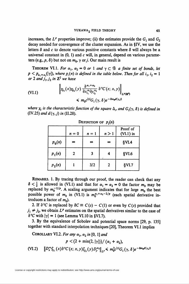
YUKAWA2 FIELD THEORY 45
increases, the Lp properties improve; (ii) the estimates provide the G, and G2
decay needed for convergence of the cluster expansion. As in §IV, we use the
letters 8 and c to denote various positive constants where 5 will always be a
universal constant in (0, 1) and c will, in general, depend on various parame-
ters (e.g.,/?, 5) but not on m0, y oij. Our main result is
Theorem VI.l. For a„ a2 = 0 or 1 and y c% a finite set oj bonds, let
P < Pai+ai(\y\)> where p¡(n) is dejined in the table below. Thenjor all ix, i2 = 1
or 2 andjx,j2 in Z2 we have
(VI.1)*,MfcO0 toffy* aYC(j; *•*)
< m0cMGx(y,8)e-Sm^y'i)
Z/(R4)
where x is the characteristic Junction oj the square A;, and Gx(y, 8) is dejined in
(IV.25) and d(y,j) in (11.28).
Definition of p¡(n)
Po(")
Pi(«)
P2(")
w = 0
3/2
«>1Proof of(VI.l) in
§VL4
§VL6
§VL7
Remarks. 1. By tracing through our proof, the reader can check that any
Ô < j is allowed in (VI.l) and that for ax = a2 = 0 the factor m0 may be
replaced by m0-2//\ A scaling argument indicates that for large m0 the best
possible power of m0 in (VI.l) is m¡¡,+ai~2/p (each spatial derivative in-
troduces a factor of m0).
2. If oyC is replaced by 5C = C(s)- C(l) or even by C(s) provided that
j\ ^ h> we obtain Lp estimates on the spatial derivatives similar to the case of
oyC with |y| - 1 (see Lemma VI.10 in §VL7).
3. By the equivalence of Sobolev and potential space norms [29, p. 135]
together with standard interpolation techniques [20], Theorem VI.l implies
Corollary VI.2. For any ax, a2 in [0, 1] and
p<(2 + xnin(2,\y\))/(ax + a2),
(VI.2) \\Dx°%t (x)dyC(s; x,y)Sh(y)D;%< m^Gx (y, a)e-*»*«*/>
License or copyright restrictions may apply to redistribution; see http://www.ams.org/journal-terms-of-use
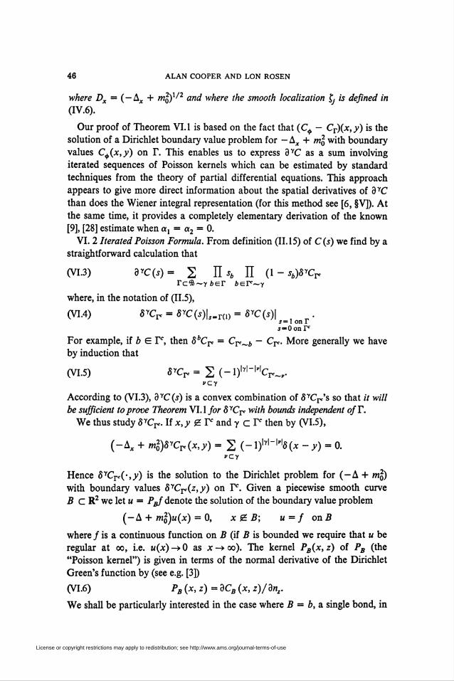
46 ALAN COOPER AND LON ROSEN
where Dx = (—Ax + ml)1/2 and where the smooth localization Çj is defined in
(IV.6).
Our proof of Theorem VI. 1 is based on the fact that (C^ — Cr)(x,y) is the
solution of a Dirichlet boundary value problem for -Ax + ml with boundary
values Cç(x,y) on T. This enables us to express 3YC as a sum involving
iterated sequences of Poisson kernels which can be estimated by standard
techniques from the theory of partial differential equations. This approach
appears to give more direct information about the spatial derivatives of 3YC
than does the Wiener integral representation (for this method see [6, §V]). At
the same time, it provides a completely elementary derivation of the known
[9], [28] estimate when ax = a2 = 0.
VI. 2 Iterated Poisson Formula. From definition (11.15) of C(s) we find by a
straightforward calculation that
(vu) dyc(s)= 2 IK II (i-í¿)SYcrrcs~yier ber~y
where, in the notation of (II.5),
(VIA) 8yCr = 8yC(s)\,„ni)=8yC(s)\s = I on Ii-Oonr0
For example, if b E Ie, then 8hCr< = Cp^ - Cn. More generally we have
by induction that
(VI.5) 8yCr= 2(-l)W"MCr*-.,.PCY
According to (VI.3), 3YC(i) is a convex combination of SYCrc's so that it will
be sufficient to prove Theorem VIA for 8yCr with bounds independent ofT.
We thus study 5YCr. If x, v £ F and y c F then by (VI.5),
(-A, + m2)8yCr(x,y) - 2 (-l)1™^* -y) = 0.vdy
Hence 8yCr(-,y) is the solution to the Dirichlet problem for (-A + ml)
with boundary values 8yCr(z,y) on Ve. Given a piecewise smooth curve
B c R2 we let u = Pgf denote the solution of the boundary value problem
(-A + ml)u(x) = 0, x J2 B; u = / on B
where / is a continuous function on B (if B is bounded we require that u be
regular at oo, i.e. u(x)^0 as *-»oo). The kernel PB(x,z) of PB (the
"Poisson kernel") is given in terms of the normal derivative of the Dirichlet
Green's function by (see e.g. [3])
(VI.6) PB(x,z)=dCB(x,z)/dnz.
We shall be particularly interested in the case where B = b, a single bond, in
License or copyright restrictions may apply to redistribution; see http://www.ams.org/journal-terms-of-use
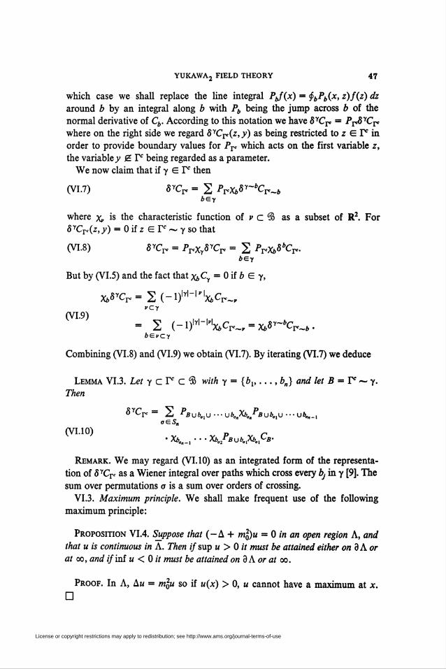
YUKAWA, FIELD THEORY 47
which case we shall replace the line integral Pbf(x) = fbPb(x, z)f(z) dz
around b by an integral along b with Pb being the jump across b of the
normal derivative of Cb. According to this notation we have 8yCr< = P^Cr*
where on the right side we regard SYCr(z, y) as being restricted to z E I* in
order to provide boundary values for Pj-c which acts on the first variable z,
the variable v E Tc being regarded as a parameter.
We now claim that if y E Tc then
(VI.7) 8yCr = 2 PrXb8y~"CT<~bbey
where Xv is the characteristic function of v c ® as a subset of R2. For
8yC?c(z, y) = 0 if z E F ~ y so that
(VI.8) SYCP = PrXyS'Cr = 2 Pr-X^r*.bey
But by (VI.5) and the fact that x¡,Cy = 0 if b £ y,
xi5^=2(-i)lYH,'lx6cr_
(VI.9)= 2 (-l)MHHX.C1.^-x.«T-4Cn-..
Combining (VI.8) and (VI.9) we obtain (VI.7). By iterating (VI.7) we deduce
Lemma VI.3. Let y cF c<& with y = {*,, ...,bn) and let B = F ~ y.
77¡e/j
8yCr = 2 PBubalU ■■•ub„XbaPiiubCiu •■• u*„„_,»es.
(VI.10) D ^•X6„n_, ■■•Xb^BuK,XbcyB'
Remark. We may regard (VI. 10) as an integrated form of the representa-
tion of 5YCn as a Wiener integral over paths which cross every b} in y [9]. The
sum over permutations a is a sum over orders of crossing.
VI.3. Maximum principle. We shall make frequent use of the following
maximum principle:
Proposition VI.4. Suppose that (-A + ml)u = 0 in an open region A, and
that u is continuous in A. Then if sup u > 0 it must be attained either on 3 A or
at oo, and if inf u < 0 it must be attained on 3 A or at oo.
Proof. In A, A« = m2,« so if u(x) > 0, u cannot have a maximum at x.
D
License or copyright restrictions may apply to redistribution; see http://www.ams.org/journal-terms-of-use
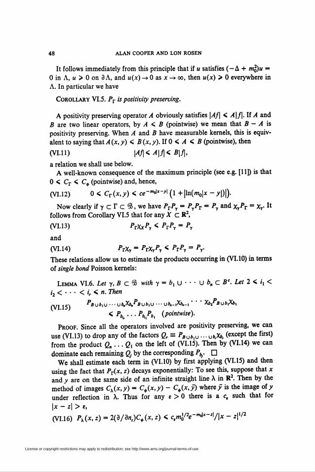
48 ALAN COOPER AND LON ROSEN
It follows immediately from this principle that if u satisfies (-A + mfyu ■
0 in A, u > 0 on 3 A, and u(x) -» 0 as x -» oo, then u(x) > 0 everywhere in
A. In particular we have
Corollary VI.5. Pt is positivity preserving.
A positivity preserving operator .4 obviously satisfies \AJ\ < A\j\. Ii A and
B are two linear operators, by A < B (pointwise) we mean that B - A is
positivity preserving. When A and B have measurable kernels, this is equiv-
alent to saying that A (x, y) < B (x, y). If 0 < A < B (pointwise), then
(VI.11) |4/|<i4|./|<*|/|,
a relation we shall use below.
A well-known consequence of the maximum principle (see e.g. [11]) is that
0 < Cr < Cq (pointwise) and, hence,
(VI.12) 0 < Cr(x,y) < ce-m^-^ (l + \ln(m0\x - y\)\).
Now clearly if y c T c ®, we have PrPy - PyPT - Py and xTPr = XY-II
follows from Corollary VI.5 that for any X c R2,
(VI.13) PTXxPy < PTPy = Py
and
(VT.14) PTXy = PrXyPy < ¿r^Y - Py
These relations allow us to estimate the products occurring in (VI. 10) in terms
of single bond Poisson kernels:
Lemma VI.6. Let y, B c $ with y - bx U • • • U ¿>„ C Bc. Let 2 < ix <
i2 < • • • < ir < n. Then
(VI 15) ¿U*iU ••• Ub,Xb.PBubtU ••• Uft»-|A^_| ' ' Xft/BuftiAi,
< ^ • • • V*. (Pointwise).
Proof. Since all the operators involved are positivity preserving, we can
use (VI.13) to drop any of the factors Qr = PBublU ... vbrXbr (except the first)
from the product Q„ ... Qx on the left of (VI.15). Then by (VI.14) we can
dominate each remaining Q} by the corresponding Pbj. □
We shall estimate each term in (VI.10) by first applying (VI.15) and then
using the fact that PT(x, z) decays exponentially: To see this, suppose that x
and y axe on the same side of an infinite straight line X in R2. Then by the
method of images Cx(x,y) = C^(x,y) - C^(x,y) where/ is the image of y
under reflection in X. Thus for any e > 0 there is a ct such that for
|x - z\ > e,
(VI.16) Px(x, z) = W/dnJC+ix, z) < ctntf2e—¿*-4/\x - z\x'2
License or copyright restrictions may apply to redistribution; see http://www.ams.org/journal-terms-of-use
YUKAWA-, FIELD THEORY 49
since Cç(x - z) ~ c(m0|x - z\)~x/2e~m(Ax~^ for large \x - z\ and similarly
for its derivatives [1].
But if T is an arbitrary subset of R2, and x is outside the convex hull
conv T of T, we let X be the straight line separating x from conv T with
d(x, conv T) = d(x, X). Then clearly Pr(x, z) = (PxPr)(x, z), and since
1-Pr/OOI < supzer[/(z)| by the maximum principle, we obtain from (VI.16):
Lemma VI.7. For any 8 < 1 there is a constant c = c(8) such that if
d(x, conv r) > j, then for any f,
(VI.17) |Pr/(*)| < ^~imorfUlConvr)sup|/(z)|.
zeT
VIA. The 3YC decay estimate of Glimm-Joffe-Spencer. We now prove the
result of [9], [28] that (VI.2) holds when a, = a2 — 0 (see Lemma II. 1 above).
As remarked after (VI.5) it is sufficient to estimate 8yCr. Consider the sum
(VI.10). To each term, call it Ta(B, y), we apply (VI.15), dropping bonds if
they touch the last retained bond. From Lemma VI.7 we get precisely the
decay factor e-imol4(Y)l as defined in (11.29) for any 5 < 1:
T„(B, y) < cWe-*^4(Y)l sup CB(z,y).
Summing over a and using (VI. 12) we obtain
(VI.18) ôYCpc < cMO, (y, «)log(l + d(y,y)~x)
where Gx is defined in (IV.25).
To extract the G2 factor we may reason as follows. Let b be any bond in y,
e.g. the one giving the maximum in (11.28). From (VI.5)
(VI.19) dyCr = 8b8y~bCr = 2 (-l)H"W8*Cn^.*CY~¿>
This represents 5YCp: as a sum of 2IyI_1 terms each of which may be bounded
by
xjpCr-tXj, < x,,PbC(r~>)~bX/2
(yU°) < ce-"""^supC<,(z,y)8h(y)zeb
by (VI.17) and the bound CB < Cr If b touches Ay2 then sup^^C^z, v) gives
a log factor as in (VI. 18); otherwise it gives a decay factor exp[- m0d(b, A^)].
Taking the geometric mean of (VI.18) and (VI.20) yields
(VI.21) X, 5YCnx,-2 < c^G, (y, 8)e-Sm^y%log(l + d(y,y)~%i
for any 8 < \. (VI.21) obviously implies (VI. 1) in the case o, = a2 = 0 with
a = 0.
VI.5. Estimates on dCB(x,y)/dy¡. To estimate (3/3y,)5YCn(x, v) we take
License or copyright restrictions may apply to redistribution; see http://www.ams.org/journal-terms-of-use
50 ALAN COOPER AND LON ROSEN
the.y,- derivative of CB in (VI. 10) and apply the maximum principle method as
in the previous subsection (using (VI.l 1)). However the log factor in (VI.21)
becomes a d(y,y)~x singularity which is not in any Lp,p > 1. It is therefore
not sufficient to use the fact that Pb is a contraction from L00 to L00 and we
must make a more careful analysis of the singularities of Pb(x, z) and
<¡CB/dy¡: In addition to the \z - y\~x singularity at z = y, dCB(z,y)/dy¡ will
have (at worst) \y — j\~x^2 singularities for j in the set e(B) of endpoints of
the individual bonds in B. More precisely:
Lemma VI.8. Given y, z in R2, and B c ^>,letj be the point in e(B) closest
toy. Thenij\z - y\ < \,
dCB(z,y) t i
<<(|737|+'*oBy,
(VI.22a)
+ \y - JV^[\ + ^ + (\y - j\+\z - j\yx/2]]
where the constant c is independent qfm0, B, z,y. If\z — y\ > \, then for any
8 E [0, 1),
(VI.22b) \oCB (z,y)/By\ < cse-Sm°^ (1 + \y - j\~x/2)
where the constant cs depends only on 8.
Remark. By (VI.6), the bonds (VI.22) apply to PB(z,y).
Proof. We first consider a special case of (VI.22a) where the Green's
function can be explicitly evaluated by conformai mapping, namely m0 = 0
and B = R+. In this case the conformai mapping f = z1/2 maps B onto R
and C ~ B onto the upper half-plane. By the method of images, the corre-
sponding Green's function is
c#W) = C$*tf, r,) = ln(|f -n\/\t - t,|)
where £ = zx'2, r, = yx'2. Since \dnfdy\ = \\y\~x/2 and |3C¿0)(Í, t\)/B-n\ <c\H — T)\~x> we thus have
(VI.23) \dC$(z,y)/dy¡\< c\y\-x/2\S - r,\~l.
The proof of (VI.22a) will then be completed by the inequality
(VI.24) \y\~1/2\S - Vfl< c[\z - y\~x +\y\-x/2(\y\ + \z\)-X/2].
To prove (VI.24) we note first that if |arg J - arg t/| > 7r/2 then |f - tj|2 >
|i|2 + |r,|2=|z| + M,sothat
(VI.25) \y\-x/2\t - r/|-1<|.vr1/2(|.y| + \z\yx'2.
On the other hand, if |arg f - arg r¡\ < 7r/2, we have
License or copyright restrictions may apply to redistribution; see http://www.ams.org/journal-terms-of-use
YUKAWA2 FIELD THEORY 61
m26, __J_2 1 U+"H|-2H' Lv|1/2i?-ijI \*-y\ M1/2I? + »ii i? +1-21.1 •
The second factor in (VI.26) has magnitude less than 1 and now |f + tj| >
(|z| + \y\)x/2; hence (VI.25) and (VI.26) imply (VI.24).
By similar conformai mapping techniques we can establish (VI.22a) for the
special case where mQ = 0 and where B = B0, a union of 0 to 4 of the
semiaxes. In this case there will actually be no |y|~1/2 singularity if y is
enclosed in an angle of it/2 or it between two axes, and only a |y|~I/3
singularity if the enclosing angle is 3tt/2. Also if B = ¿?,, a union of 0 to 4
unit bonds emanating from the origin, and if the origin is the closest lattice
point toy, conformai mapping shows that
(VI.27) \dCB»(z,y)/dy¡\<c\y\-x/2
provided |z| > 1 so that z is bounded away from 0 andy.
Consider now the case of general B c ©. If / is the lattice point closest to
y, we let J5, be the set of unit bonds in B touching y and BQ the union of the
rays in 2?, extended fromy to oo. Then since 5. c B we have Cj0) = CB0)-
P$»C$* as in §VI.2. Similarly Cjg = Cj°> - P^C^ so that
(VI.28)
Cf\z,y) - C$!(z,y) -/ dx PB®(z, x)CB°?(x,y)
-f dxPB°Xz,x)CB*(x,y).JB~Bl
On the right side of (VI.28), the variable x satisfies \x — j\ > I so that
differentiating (VI.28) with respect to y,- and using (VI.27), we can dominate
the right side of (VI.28) by c|y — j\~x¡2 by the maximum principle. It follows
from (VI.28) that C^\z,y) satisfies the bound (VI.22a):
(VI.29)
^ |< <{ ̂ +\, -Jf'V + <\> -A^-A)-"1}}-
Next we extend this result to m0 > 0 by means of the resolvent formula
,yT,m *c*(*>y) *ciB%'y) 2fr, Jc{B°Xx*y) j2^•^ —3^-3^-W°J C*(z> x) tfy, dx-
Using the bounds (VI.29) and CB < Cr we find that the right side of (VI.30)
can be dominated by
(VI.31) cm20jC+(z,x){\x -y\~x +\yfX/2[l + (M + |y|)~'/2]} d2x
where we have set / = 0. By making the change of variable £ = mQx, we can
estimate (VI.31) by c(m0 + mxn/2/\y\x/2) where the constant c is independent
License or copyright restrictions may apply to redistribution; see http://www.ams.org/journal-terms-of-use
52 ALAN COOPER AND LON ROSEN
of m0. Thus from (VI.29) and (VI.30) we obtain
ZCB(y,z)
9y,-< <{ ]737| +"o + br1/2[i + <12 + (\y\ + \AVl/2]}
as desired.
Finally, (VI.22b) follows from (VI.22a). For let D be the disk of radius e
and centre>>. Then in R2 ~ D ~ B, u(z) = dCB(z,y)/dy¡ satisfies
(VI.32) u(z)~f 1BuBD iz,x)ZCB(x,y)
dx.
Consequently by (VI.l 1) and (VI. 14)
<>CB(x,y)
(VI.33)
«W| < / PBD {', x) to, dx
< ce-am°^-y\-c)[e-x + m0+\y -;r'/2(l + ™x0/2 + £~x/2)]
for any a < 1, where we have applied Lemma VI.7 and (VI.22a). Clearly
(VI.33) implies (VI.22b) (the powers of m0 can be absorbed in the exponential
decay factor). □
VI.6. Estimates on d8yCr(x,y)/dy¡. When y is empty, the estimate (VI.l)
for 3Crc/3^, follows immediately from (VI.22). We move to the case where
|y| = 1, i.e. y consists of a single bond b. Now by (VI. 10) and (VI.15)
<[dzPb(x,z)Jh
(VI.34) ±8»Cr(x,y)3v,
CB(z,y) = I(x,y)
where B = Tc ~ b. If b does not touch A^, then |z - y\ > 1 in (VI.34) and we
may apply (VI.22b) to bound dCB/dy¡ and (VI.17) to bound Pr. In this way
estimate (VI.34) by (inserting x, (x) and Xj (y))
(vi.35) /(x,7)x,iWx,2(>') < «MfctofcOO»-*"**^! +|^ -y0|"1/2)
where 5 < 1 andy0 is the point in e(5) closest toy. Clearly, (VI.35) is in L*~
(i.e. in any Lp,p < 4) with the bound (VI.l) on its Lp norm. Sincepx(l) = 3
< 4 we have established Theorem VI.l for this case.
Suppose next that b does touch AJ2. We may assume that the origin is at an
end of b touching A^ and that the origin is the point of Z2 closest toy (if not
we have the bound (VI.35) as above). Suppose that xx labels the coordinate
parallel to b (xx> 0 on b) and x2 the perpendicular coordinate. Then by
(VI.22a) we have
(VI.36) \oCB (z,y)/dy,\ < c[f(z,y) + g(y; m0)],
where
(VI.37a) f(z,y) = \z -y\~x + \y\~x'2(\y\ + \z\yx/2
License or copyright restrictions may apply to redistribution; see http://www.ams.org/journal-terms-of-use
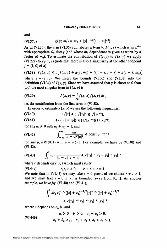
YUKAWA, FIELD THEORY 53
and
(VI.37b) g(y, m0) = m0 + \y\~x/2(l + mx¿2).
As in (VI.35); the g in (VI.36) contributes a term to I(x,y) which is in L4-
with appropriate G2 decay (and whose mQ dependence is given at worst by a
factor of m0). To estimate the contribution of f(z,y) to I(x,y) we apply
(VI.22a) to Pb(x, z) (note that there is also a singularity at the other endpoint
/ = (1,0) of b):
(VI.38) Pb(x, z) < c[f(x, z) + g(z; m0) + f(x - j, z - j) + g(z - j; mQ)]
where z = (z„ 0). We insert the bounds (VI.36) and (VI.38) into the
definition (VI.34) of I(x,y). Since we have assumed that y is closer to 0 than
to/, the most' singular term in I(x,y) is
(VI.39) J (x, y) = ff(x, z)f(z, y) dzxJb
i.e. the contribution from the first term in (VI.38).
In order to estimate J(x, y) we use the following inequalities:
(VI.40) l/|x| <(l/\xx\°>)(l/\x2\°>),
(Vi.41) \/{\x\ + \y\)<(i/\xxr)(l/\xp),
for any a¡ > 0 with ax + a2 = 1, and
du
\u - vY\u\"
for any p, q E (0, 1) with p + q > 1. For example, we have by (VI.40) and
(VI.42),
(^ /„' dz-|x-z||z-y| < clx*nxx -*™~'
where c depends on r, j, t which must satisfy
(VI.44a) r, s, t > 0, r + s + t = I.
We note that in (VI.43) we may take s = 0 provided we choose r + t > 1,
and we may take r = 0 if xx is bounded away from [0, 1]. As another
example, we have.by (VI.40) and (VI.41),
/1i/z1zr'/2(w + zI)-1/2|y|-1/2(bl + ^)",/2•'0
< c|xI|-"1x2|-^|y1|-61y2|-^
where c depends on a,, b¡, and
a¡ > 0, b¡ > 0, ax + a2> 0,
¿>i + ¿2 >i> 0, + ö2 + bx + b2 > 1.
<™2> ri7^w<const|üi,_í,"?
(VI-44b) . ^ 0
License or copyright restrictions may apply to redistribution; see http://www.ams.org/journal-terms-of-use
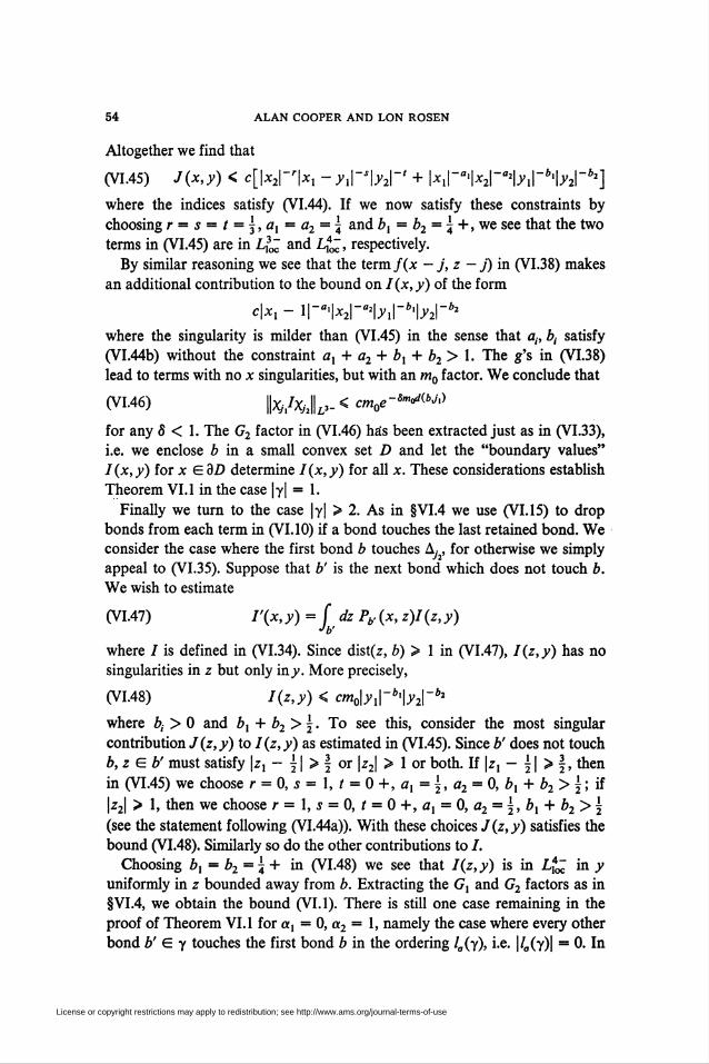
54 ALAN COOPER AND LON ROSEN
Altogether we find that
(VI.45) J(x,y) < c[\x2r\xx~yxr\y2\-> + |*,|—|*2r«»|*r*'M-*]
where the indices satisfy (VI.44). If we now satisfy these constraints by
choosing r = s = t = \,ax = a2=\ and bx = b2 = \ +, we see that the two
terms in (VI.45) are in Lx~ and Lf^, respectively.
By similar reasoning we see that the texmf(x — j, z — j) in (VI.38) makes
an additional contribution to the bound on I(x, y) of the form
c\xx - l\-^\x2\-^\yx\-b^\y2\-^
where the singularity is milder than (VI.45) in the sense that a¡, b¡ satisfy
(VI.44b) without the constraint ax + a2 + bx + b2> 1. The g's in (VI.38)
lead to terms with no x singularities, but with an m0 factor. We conclude that
(VI.46) |x,/X,-2||L3-< cm0e-Sm^b^
for any 5 < 1. The G2 factor in (VI.46) has been extracted just as in (VI.33),
i.e. we enclose b in a small convex set D and let the "boundary values"
I(x,y) for x EdD determine I(x,y) for all x. These considerations establish
Theorem VI.l in the case |y| = 1.
Finally we turn to the case |y| > 2. As in §VI.4 we use (VI.15) to drop
bonds from each term in (VI. 10) if a bond touches the last retained bond. We
consider the case where the first bond b touches A,, for otherwise we simply
appeal to (VI.35). Suppose that b' is the next bond which does not touch b.
We wish to estimate
(VI.47) I'(x, y) = fdz Pb, (x, z)I (z, y)Jb'
where / is defined in (VI.34). Since dist(z, b) > 1 in (VI.47), I(z,y) has no
singularities in z but only iny. More precisely,
(VI.48) I(z,y) < cm0\yx\-b^\y2\-^
where b¡ > 0 and bx + b2>\. To see this, consider the most singular
contribution J(z,y) to I(z,y) as estimated in (VI.45). Since V does not touch
b,z Eb' must satisfy |z, - \\ > \ or |z2| > 1 or both. If \zx — \\ >f, then
in (VI.45) we choose r = 0, í = 1, t = 0 +, ax = \, a2 = 0, bx + b2 > \ ; if
|z2| > 1, then we choose r = 1, s = 0, t = 0 +, ax = 0, a2 = \, bx + b2 > 5
(see the statement following (VI.44a)). With these choices J(z,y) satisfies the
bound (VI.48). Similarly so do the other contributions to /.
Choosing bx = b2—\+ in (VI.48) we see that I(z,y) is in Lx^ in y
uniformly in z bounded away from b. Extracting the Gx and C72 factors as in
§VI.4, we obtain the bound (VI.l). There is still one case remaining in the
proof of Theorem VI.l for a, = 0, a2 = 1, namely the case where every other
bond V E y touches the first bond b in the ordering la(y), i.e. |/„(y)| = 0. In
License or copyright restrictions may apply to redistribution; see http://www.ams.org/journal-terms-of-use
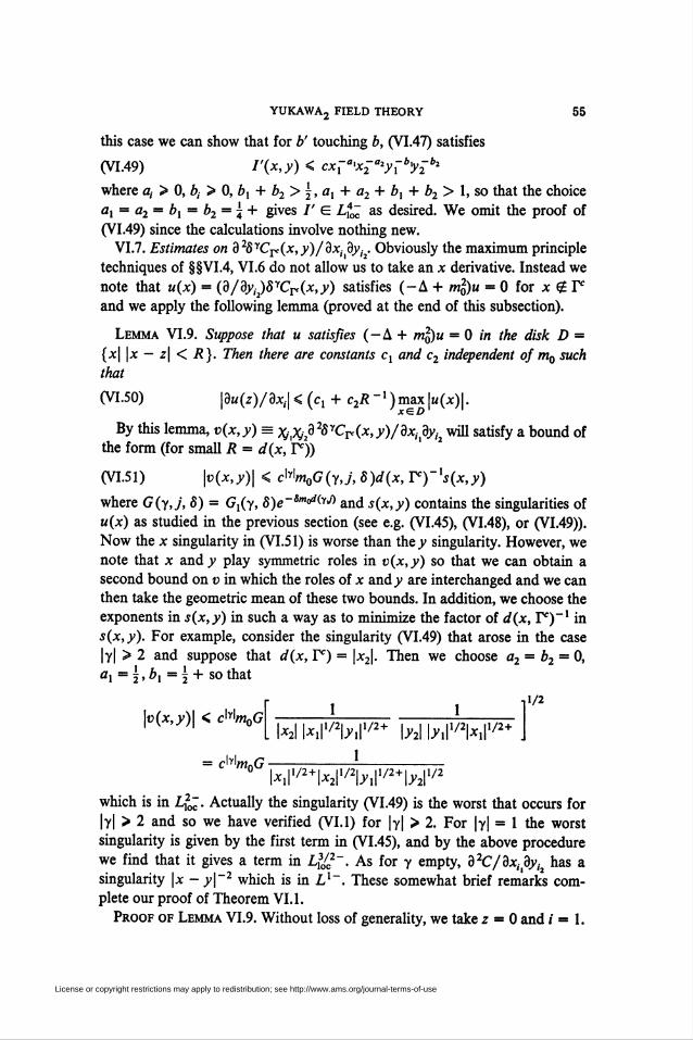
YUKAWA-, FIELD THEORY 55
this case we can show that for V touching b, (VI.47) satisfies
(VI.49) I'(x,y) < cxx-"<x2-aiyx-by2-b>
where a¡ > 0, b¡ > 0, bx + b2 > \, ax + a2 + bx + b2 > 1, so that the choice
ax = a2 = bx = b2 = \+ gives /' E Lx~ as desired. We omit the proof of
(VI.49) since the calculations involve nothing new.
VI.7. Estimates on d28yCr(x,y)/dx¡dy¡2. Obviously the maximum principle
techniques of §§VL4, VI.6 do not allow us to take an x derivative. Instead we
note that u(x) = (3/3y,2)5YCP(x,y) satisfies (-A + ml)u = 0 for x $ F
and we apply the following lemma (proved at the end of this subsection).
Lemma VI.9. Suppose that u satisfies (—A + ml)u = 0 in the disk D =
{x\ \x — z\ < R). Then there are constants cx and c2 independent of m0 such
that
(VI.50) \du(z)/dx¡\< (c, + c^-^maxlM^)!.
By this lemma, v(x,y) = X/lXj^2SyCr(x,y)/dxidyii will satisfy a bound ofthe form (for small R - d(x, F))
(VLSI) \v(x,y)\ < c^m0G(y,j, 8)d(x, F)-Xs(x,y)
where G(y,j, 8) = G,(y, 8)e~Sm,fi(yJ) and s(x,y) contains the singularities of
u(x) as studied in the previous section (see e.g. (VI.45), (VI.48), or (VI.49)).
Now the x singularity in (VI.51) is worse than they singularity. However, we
note that jc and y play symmetric roles in v(x,y) so that we can obtain a
second bound on v in which the roles of x and y are interchanged and we can
then take the geometric mean of these two bounds. In addition, we choose the
exponents in s(x,y) in such a way as to minimize the factor of d(x, F)~x in
s(x,y). For example, consider the singularity (VI.49) that arose in the case
|y| > 2 and suppose that d(x, F) = |x2|. Then we choose a2 = b2 = 0,
a\ = 2 » *i = \ + so tnat
,1/2
\v(x,y)\ < c^m0G1 1
j \xxnyx\x/2+ \y2\ \yinXl\^* J
= MmM-0 W,/2+W1/2b1l1/2+b2l,/2
which is in L,2". Actually the singularity (VI.49) is the worst that occurs for
|y| > 2 and so we have verified (VL1) for |y| > 2. For |y| = 1 the worst
singularity is given by the first term in (VI.45), and by the above procedure
we find that it gives a term in L\¡2~. As for y empty, 32C/3x(i3yÍ2 has a
singularity |* - y|-2 which is in Ll~. These somewhat brief remarks com-
plete our proof of Theorem VI. 1.
Proof of Lemma VI.9. Without loss of generality, we take z = 0 and / = 1.
License or copyright restrictions may apply to redistribution; see http://www.ams.org/journal-terms-of-use
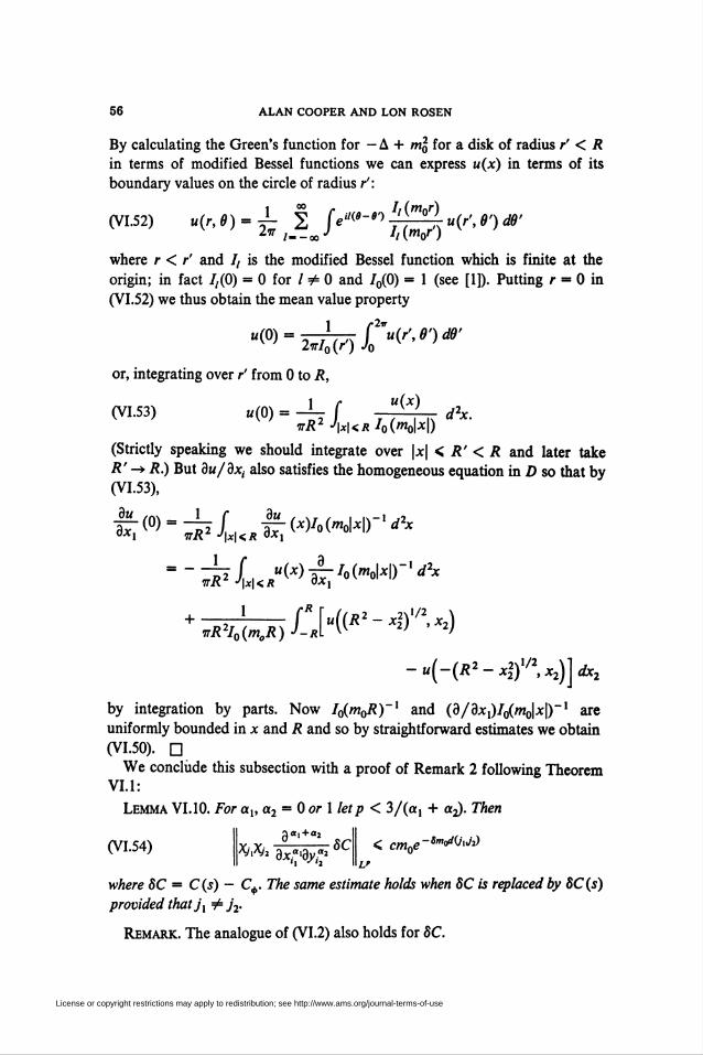
56 ALAN COOPER AND LON ROSEN
By calculating the Green's function for - A + ml for a disk of radius r' < R
in terms of modified Bessel functions we can express u(x) in terms of its
boundary values on the circle of radius r':
(vi.52) «M)-¿ 2 ¡eiKe-9')T^uV>e')d9'Lm /--oo-7 Jt(mor)
where r < r' and I, is the modified Bessel function which is finite at the
origin; in fact 1,(0) = 0 for / ^ 0 and 70(0) = 1 (see [1]). Putting r = 0 in
(VI.52) we thus obtain the mean value property
ox, integrating over r' from 0 to R,
i r u(x)(VI.53) «(0) = 4l f ii ■ .x d2x.
irR2 J\x\<.Rl0(mQ\x\)
(Strictly speaking we should integrate over |jc| < R' < R and later take
R' -* R.) But du/dx, also satisfies the homogeneous equation in D so that by
(VI.53),
■-¿4</wi/«KWr,A
+ ^- (R\u((R2-x2)1/2,x2)irR%(m0R)J-Rl ^ 2) 2>
-u(-iR2-x2)1/2,x2)]dx2
by integration by parts. Now 70(moiî)_1 and id/dxx)I(j(mQ\x\)~x aie
uniformly bounded in x and R and so by straightforward estimates we obtain
(VI.50). DWe conclude this subsection with a proof of Remark 2 following Theorem
VI.l:
Lemma VI.10. For a„ <x2 = 0orlletp < 3/(a1 + ctj. Then
(VI.54) Wfc dx">dy,a> sc < cm0e-Sm°d(J«'l)
L*
where 8C = C(s) - Cr The same estimate holds when 8C is replaced by 8C(s)
provided thatjx ¥* j2.
Remark. The analogue of (VI.2) also holds for 5C.
License or copyright restrictions may apply to redistribution; see http://www.ams.org/journal-terms-of-use
YUKAWA2 FIELD THEORY 57
Proof. By (11.15) SCis a convex combination of differences Cr = Cy-C^
so that it suffices to prove (VI.54) for 8Cr. But as in §VI.3,
(VI.55) |5CT.| = |PrC,| = 2 PrX,C<, ; 2 pbc*-bev
The sum in (VI.55) converges because of the exponential decay of Pb or C^.
We can estimate y derivatives of (VI.55) as in §VI.6 for |y| = 1 and x
derivatives as above in order to obtain (VI.54).
If/i *h then itis easv t0 check using (VI.40) - (VI.41) that (VI.54) holdswith 8C replaced by C,.: the |jc - ^|_ai~ai singularity of
(3a'+ay9x)°l3y^)C<()(x,y) is in Lp withp < 3/(a, + a2) since x and y are in
different lattice squares. Hence (VI.54) must hold for C(s) = 8C + Cr □
VI.8. A decomposition lemma. The major role played by Theorem VI. 1 is to
control 5 derivatives dyS of fermi covariances. However, the following con-
sequence of Theorem VI. 1 is used to control 5 derivatives of boson covari-
ances (see (IV.27)):
Lemma VI.ll. Suppose \y\ > 2,p < oo, e < 1. There exist positive operators
Cy>± on L2(R2)such that dyC = Cy+ - Cy>_ with
(VI.56) \\Cy,±\\L,<cMm0Gx(y,8)
and
(VI.57) ||Z>£Cy)±Zr||L2< c^m0Gx (y, 8).
Proof. Let B = DedyCDe. If {^} is a smooth partition of unity, we see
from Corollary VI.2 that
(VI.58)<m¡c^Gx(y,8).
That is, B is a Hilbert-Schmidt operator on L2(R2). Thus fi±, the positive and
negative parts of B (in the operator sense), also satisfy the bound (VI.58). We
define Cy>± = Z)_e5±Z)-e so that 3YC = Cy>+ - Cy_ and Cy± satisfy
(VI.57). But (VI.57) implies (VI.56) by the following lemma. □
Lemma VI. 12. Let
q~x <r~x + e/2 where0 < e < 2.
Then D~tD~t is a bounded operator from Lq (R4) to Lr(R4) with norm bounded
by cmö^e/2+r"-''"\
Proof. D ~e is given by convolution with a function ml~ed_e(m0\x\) which
is exponentially decreasing at oo and has a singularity \x\'~2 at x = 0. Thus
foranyp < 2(2 - e)_l,
License or copyright restrictions may apply to redistribution; see http://www.ams.org/journal-terms-of-use
58 ALAN COOPER AND LON ROSEN
(VI.59) |K-eKM)IUtf) < cmö2/p.
Therefore, by Young's inequality,
¡D-'D-Vfry)^ < cmo4-2-4^'^!^^
where z?"1 + q~x = 1 + r~l and q~x - r~x < 1 + (e - 2)/2 = e/2. D
VII. Estimates.
VII. 1. Introduction. In this section we establish the estimates used in §§III
and IV. In particular, in §VII.2 we study the operators K(s), dyK(s), and
8K(s) = K(s) - K(l) on % = %/2 © %x/2 and show that they are in
certain Qpq.s classes (defined in (III. 12)). In §VII.3 we obtain estimates on
quadratic expressions such as B (s) (defined in (III.8)). In §VII.4 we prove the
"linear lower bound" for pA(s). Our method of proof is basically that of
McBryan [16] in that it involves momentum expansions but we obtain a
considerable simplification by using the formalism of §111 to control the
terms in the expansion. Finally we use the estimates of §§VIL2-VIL3 to
complete the proof of decoupling at s = 0 (in §VII.5) and to justify the
formulas for s derivatives (in §VII.6).
There is a basic complication involved in the estimates for s B.C. In Seiler
[22] and subsequent work on Y2 frequent use was made of the elementary
identity
(VII.l) (-#• + m0) C if + m0) - 1
for C = Cq. Since C(s) is not diagonal in momentum space, (VII.l) is not
available for s B.C. when s ¥= I. As a replacement for (VII.l) we shall
systematically write
C(s) = C+ + 8C(s).
We then use (VII.l) on the C^ term and the local Lp estimates of the previous
section on the 5C term, exploiting the fact that d28C(s)/dx,dyj has better Lp
properties than d2C(s)/dx,dyj (see Lemma VI.10).
VII.2. Properties oj K. In this section we study the operator-valued function
oi<t>,
(VII.2) K (A, s) = S0 (s)<¡>Xa = C (s)(p- + m0)<j>xA,
as well as the related operators 8K and dyK defined as in (VII.2) but with
C(s) replaced by 8C(s) and dyC(s), respectively. We intend to calculate
products, adjoints, and traces of these "operators" using their integral kernels,
e.g.,
(VII.3) Tx%(K8K) = ftx K(x, y)8K(y, x) dx dy
where tr denotes the trace over spinor indices. Why are such operations
License or copyright restrictions may apply to redistribution; see http://www.ams.org/journal-terms-of-use
YUKAWAj FIELD THEORY 59
justified? In certain cases, e.g. in the calculation of Tr|5.Kj2 as in Lemma
VII. 1, we are justified in the use of a formula like (VII.3) because we can
show that SK is Hilbert-Schmidt on % for almost all <f>. But this assertion that
8K E (^(X) a.e. or the identity (VII.3) must ultimately be justified by
passing to momentum cutoff objects:
(VII.4) KoAA's) = S0,(^kXa
where a denotes the fermion and k the boson cutoff, 50a is defined in (III.9),
and <bK(x) = f<p(y)hK(x - y) ay in terms of the same smooth function h used
in (III.9).
Since KaK, 8KaK are Hilbert-Schmidt we are justified in using formulas like
(VII.3) with a, k < oo and we then pass to the limit a, k = oo. In a number of
the following calculations where this limiting procedure is fairly clear we shall
simply deal directly with the case a, a — oo. However, we wish to emphasize:
expressions like B = \ :Tx(K2 + KyK): or :Tt(K + K*)2: have no meaning
independent of the limiting procedure a -» oo.
For y = (J1J2) e Z4 and e = (e,, e^ E R2, we introduce
(VII.5) TeJ = DHjKxjD»
as well as the related operators dyTeJ and 8TcJ in which K in (VII.5) is
replaced by dyK and 8K, respectively. Operators such as (VII.4) and (VII.5)
are linear in <f>. If Tx,..., Tr are r such operators on % then Tr^T,... Tr)
will have the form fw(xx,..., xr)<b(xx)... <b(xr) dx; we refer to w as the
kernel of Tr^T, ... Tr). We use the notation Lp~ to denote the functions in
Lq for any q <p; when we write ||w||£,- < c we mean that ||>v||¿, < c(q) for
q < p, where c(q) may diverge as q -»/>. The following two lemmas are basic
to this section.
Lemma VII.l. Given e„ e2 < \, letp0 = 12/(11 + 6 max(e„ e2, - |)).
(a) The kernel w of \\dyTeJ\\22 = Tr(3Yr£*.3Yrti/) is in LP»-(R4) and
(VH.6a) ||w||L,0_ < cm£Gx (y, 8)e-Sm^yA
(b) The kernel w of \\8TeJ\\l is also in Lp°- with
(VII.6b) IMU-< cm^e-Sm^^\
Remarks. 1. We are using the same notation as in the previous sections:
c, a, and 5 will represent various positive constants as explained after (IV.6);
G, is defined in (IV.25), d(y,j) in (11.28), and dfJuJi) in 0V.42).2. Assuming that A,2 c A (otherwise TeJ = 0), we can omit the Xa in
K(A, s).Proof, (a) Recalling that the adjoints T* on %x/2 and Ty on L? are related
by T* = D - xTyD, we have
(VII.7) Tr(3Yr*3Yr£i/.) = Tr(D ~i+2^dyS% px+2*%.dySx,<t>).
License or copyright restrictions may apply to redistribution; see http://www.ams.org/journal-terms-of-use
60 ALAN COOPER AND LON ROSEN
Letting p2 be multiplication by m0, we see from (VII.7) that w(x,y) is given
by a sum over i, /' = 0, 1,2 of terms of the form
(VII.8) cu,D -x+2t*(x- y)(B?D '+2"B,. )(x, y)
where Da(x - y) is the kernel of the operator Da, c„, is a constant arising
from the trace over spinor indices, and B, is the operator with kernel
(VII.9) B,(x,y) - f,i(x)(3^Q,,)(x,>')x,2(7)
where;?, acts on the argument y of 3YC.
If we now write
2
(VTI.10) i)l+2t'=2ftfl-1+\*=o
then (VII.8) becomes a sum of terms of the form
(VII.l 1) b,r,.D-x+2"(x -y)fq~(x^x)D-x+:u'(x' - y')Ck,(y',y) dx'dy'
where Q, = />*£;,( 3 YÇp,)x,v When fc = 0, 1, thepk = /'3/3xK in Ck, acts either
on dyC(x,y) or on ^ (x), but in either case we know from Theorem VI.l that
for any r < §,
(VII.12) ||Q,,-|Ur«) < <C|Y|C7, (y, 8)e-Sm^yA
But the x' andy' integrations in (VII.l 1) take place over a finite area, so that
we can bound the L*(R4) norm of (VII.l 1) by
c{/|Q,.(x',x)|>-1+2^(x-7)i)-1+2"(x'-/)f
(VTI.13) • \CU (y',y)\P dx dx' dy dy'j
<^II^IL'IIQHI^||^-1+2ii(-)IL,(R2)||ö-,+2£'(-)||L,(R2)
if 2/r + l/q = 2/p. In (VII. 13) we have applied Young's inequality exploit-
ing the fact that D ~"(x - y) is a function of the difference x - y. By (VI.59)
(VII.14) ||Z> ~a\\L,< oo if q < 2/ (2 - min(a, 2))
so that in (VII.13) we must take q < 2/(1 + 2 max(e„ e2, - ¿)) and r <
3/2. Thus if we choose p < 12/(11 + 6 max(e,, e2, - £)), (VII.12) and
(VII.13) imply (VII.6).(b) If 3 YC is replaced by 5C, we argue as in (a) using Lemma VI. 10 in place
of Theorem VI.l. □
Lemma VII.2. (a) Let w be the kernel oj Tx(KXj8Kx,), or Tx(8Kx¡8KXj2).
Thenjorp <f,
(VII.15) IML'< cw0oe-Sm°d(/"/j).
License or copyright restrictions may apply to redistribution; see http://www.ams.org/journal-terms-of-use
YUKAWA, FIELD THEORY 61
(b) Let w be the kernel ofTr(dy2Kxj dy,Kxj) where yx is nonempty. Then for
P<h2
(VII.16) ||h>||l,< cmS II G, (yk, 8)e-Sm^y^.k-l
Proof, (a) The more singular case is Tr(iÇx; 8Kxj ) with kernel
w(*,y) - ^,(%(7)tr(S()', x)8S(x,y)).
By Theorem VI.1 and Lemma VI. 10, S and 8S are in L2~ and L3~,
respectively, so that by Holder's inequality, w E L6//5~ with norm bounded
as in (VII. 15).
(b) Same proof as (a). □
Remark. By the inclusion, 6p¡ c QPl ifpx < p2, for the trace classes Qp(%)
on %, we can obtain information about 6,n norms from Lemma VII. 1. For
example, with e„ e2 < \,
(VII.17) \\STtJ\(i<\\8Tj42=fw(xx, x2)w(x3, x4)4>(xx)... <f>(x4) dx
where the kernel in (VII.17) is in LP(RS) if p < p0 with norm 0(e~Smod(J,Jli).
The next two lemmas collect some useful criteria for certain operators to be
bounded on L*(R2) or to be in Qp(L2), the trace ideal on L2(R2) with norm
\\A\\p = TT(AUy/2.
Lemma VII.3. Suppose l< p < oo; a, ß E R; and I E C0°°(R2).
(a) 3D ~x/dxk is a bounded operator on LP(R2).
(b) DaÇD-" is a bounded operator on LP(R2) and the norm ofx¡D%D "° on
Lp(R2)isO(e-*m^iJ)).
(c)IfO<a< ß/2 and a < 1/2 then DaXjD ~B is a bounded operator on
L\R2) and the norm ofXiDaXjP> ~ß " 0(e-&m^iJy).
Proof, (a) This follows from [29, Theorem V.3].
(b) Forp = 2 the boundedness of Da$D ~" was established in [21, Lemma
6.1]. The same proof works for general p (using part (a)). As for the decay,
suppose i/(A,, A7) > 0. If a > 0 we choose an integer n > a/2 and we write
(VII.18) %£>% = XiD2nDa-%
Now D2n = (-A + /Kq)" is a local operator and we know that for x E A„
y E supp tj, the kernel D"-2n(x - y) is 0(<?-s",ol*-.>'l) together with all of its
derivatives. Thus the norm of (VII.18) on Lp is 0(e-&m^(iJ\ If a < 0, we
write
X¡D%D -" = x¡D%D2nD -2"-"
and repeat the above argument with D2n acting to the left.
(c) The boundedness of DaXjD ~ß was established in [21, Lemma 6.2]. We
License or copyright restrictions may apply to redistribution; see http://www.ams.org/journal-terms-of-use
62 ALAN COOPER AND LON ROSEN
obtain the exponential decay as in part (b). □
Lemma VII.4. Let 2 < p < oo; a, ß E R;/ G L"(R2); and f G C0°°(R2).(a) IJß>2p-x, thenjD-* G Gp(L2).(b) IJß - a > 2p~x then DaÇD ~B E ßp(L2).
(c) IJß -2a> 2p~x then DaXjD ~B E Gp(L2).
Proof, (a) This is a special case of Lemma 2.1 of [24].
(b) Letting {£,} be a partition of unity where each |(- is a translate of a fixed
| G C0°°, we write
Da$D ~B - 2 (Da$D -* ){D -U-%).
i
By Lemma VII.3(b) the first factor is bounded, and by (a) the second factor is
in Qp, so that each term in the sum is in &p. The sum converges in Qp since if
d, = dist(supp I, supp £,) > 1, (CD-ߣ,)(x,y) is 0(e-Sm<A) along with all of
its derivatives so that the Hilbert-Schmidt norm \\DaW~ßii\\e1 is 0(e~Sm^).
Finally, Gp D 0^.(c) We choose ß' to satisfy 2a < ß' < ß - 2p~x and we write DaXjD ~B
= (DaXjD -*) • (DB'$jD ~B). The first factor is bounded by Lemma VII.3(c)
and the second factor is in Qp by part (b). □
We return to estimates of the type in Lemmas VII.l and VII.2 for the case
s= 1:
Lemma VII.5. (a) For ex,e2> —\,let
px = (l -min(e[, ~) - min(e2, i)) .
There is a Junction w G Lp(R4)jor any p < px such that
(Vn.19) \\T-tJ(l)f2<fw(xx, x2)<t>(xx)4>(x2) dx
Jor almost all $ and
(VII.20) \\w\\l'< ce-S"1«1^.
(b) If ex = 0 and 0 < e2 < \, let p2 = \(l + e2)_1. There is a function
w E LP(RS) satisfying (VII.20) for any p < p2 such that for almost all d>,
(VH.21) \\TtJ(l)\\<jw(xx .. . x4)<t>(xx) .. . <J>(*4) dx.
Remark. With a little more work it is possible to prove (VII.20) for the
actual kernels of ||r_£i/(l)||2 and ||r£</.(l)|^, but the stated result suffices for
our purposes.
Proof, (a) If d(jx,jf) — 0 we can eliminate the smooth localization ^:
License or copyright restrictions may apply to redistribution; see http://www.ams.org/journal-terms-of-use
YUKAWA2 FIELD THEORY 63
F-« W& < \\D ~%P'f\\D ~tlKmP "IE
<c|Z)-^(l)x,,Z)-«i2
by Lemma VH.3(b). The kernel of the right side,
"(*„ x2) - c%¿x¡)D-1"2" (xx - xàtfxàD-1-** (x2 - xx)
is easily seen to be in Lp,p < px by (VII.14).
If d(jx,j2) > 0 we retain the ^ and take w = ker|| r_ei/(l)||2. The estimate
(VII.20) follows from the fact that for y E Ah, $h(x)C(l; x - y) is a C00
function which is 0(e~SmoáUlJ:í) together with all of its derivatives.
(b) As in part (a), for ¿(/„/j) = 0 we use ||re,(l)||4 < UjUK^D^,
and for d(jx,j2) > 0 we appeal to the smoothness and decay of ÏjC^. □
If we intergrate (VII. 19) with respect to dp, and apply Holder's inequality,
we see that forp < /?,,
(VII22) HT-jW&fa <jy{xx,x2)C(s;xx,x2)dx
It follows from (VII.22) that Ä"(1)Z) "' E ßj2;i for any e > 0. Similarly from
(VII.21) we see that K(l)D' E 644;, for any e < \. Using complex interpola-
tion, we can obtain the well-known results [23] that
(VII.23) K(l)ECPt„., if p > 2, ? < oo.
It is clear from Lemma VII. 1 that dyK and 8K have better 6 ;j properties
than K(l) in the sense that the restriction p > 2 can be improved. For
example, by the same argument as in (VII.22), if e,, e2 < \,
(VII.24) \\*yTj2¡2.,< cmSGx (y, i)e-*^^.
This implies
Corollary VII.6. For any p>\,q < oo,
(VII.25) |i},*T**,U.* cwôG'<* «)'"îmod(W).
(VII.26) |i}.M&6»U.< cmo-e-*"«^"*>.
Remark. Writing K = 8K + K(l) we see by (VII.26) that K(s) enjoys the
same Qpq properties as #(1), e.g. ifp > 2, q < oo,
(VH.27) |&*tofcU.< ^o^^0'^-Proof. If e, = e2 = e < ¿ we write
(VII.28) WKxj, = (^^)(dyTtJ)(D-%2)
where £ E C™ covers ^, i.e., ÇÇJt = ¡Jt. Now the operator CD~e on % is
unitarily equivalent to D X/2ÇD -e-1/2 on iJCo, which by Lemma VII.4(b) is in
License or copyright restrictions may apply to redistribution; see http://www.ams.org/journal-terms-of-use
64 ALAN COOPER AND LON ROSEN
Qq for any q > 2/e; similarly for D %.. Hence by Holder's inequality
(VII.29) |fr»'*fcU.< c^rrj^where/>"' = 2~l + 2q~x; i.e. (VII.29) holds ioxp > ({■ + e)~x. Since e may
be chosen arbitrarily close to ¿, the restriction on p in (VII.29) is p > f.
(VII.24) and (VII.29) imply (VII.25) for q = 2 and by a standard hypercon-tractivity argument [11] for any q < oo (of course the constant c in (VII.25)
diverges asp -> § or q -» oo). The proof of (VII.26) is virtually identical. □
We now have the technical tools in hand for the
Proof of Lemma IV.5. (i) is just Lemma VII. 1(a). (ii) follows from a slight
modification of (i): in (i) we replace £ by £ where {£,} is a suitable partition
of unity and then we sum over i, the exponential decay giving convergence.
(iii)-(v) are all proved by writing K = 8K + K(l) and using the triangle
inequality to estimate the two resulting terms separately. The Ä"(l) term is
estimated by Lemma VII.5 and the 8K term by Lemma VII.l(b) and (VII.17).
DIn §VII.4 we shall require the following information about the limit
K = lim^A, (KK is defined by (VII.4) with o = oo):
Lemma VII.7. Let p > 2, q < oo. There are positive constants c and e such
that jora > 1,
(VII.30) ||A-(A, s) - KK(A, s)\\pq;i< cm^-.
Proof. We verify (VII.30) by following through the proof of (VII.27)
(based on (VII.23) and (VII.26)) with </> everywhere replaced by 8<t>K = 4>- $K.
When we calculate ||(A: - KJD-'\\22;i as in (VII.22) we find that C(s) is
replaced by differences such as
(VII.31) $C$-h;$C£ or SC$*hK - h^Ct*hK
where we are entitled to insert £ G Cq0 provided £ = 1 on a sufficiently large
set. (Notation, h* acts on the first and *hK on the second variable of
$(xx)C(xx, x2)$(x2).) By part (a) of the following lemma, these differences go
to zero in any Lp(R4),p < oo, at a rate 0(k~') and this establishes (VII.30).
D
Lemma VII.8. (a) Let ? G C0°°(R2), let hK be defined as in (III.8), and let dK
be one oj the junctions in (VII.31). Then jor any p < oo, there is an e > 0 such
that K||L, = 0(k-°).
(b) Ijax, a2 < 1 with ax + a2 < §, there is an e > 0 such that
(VII.32) WD"'^(C - h;C)$jDa>\ < cmZK-te-Sm*t<J^)
where \\ • || denotes the operator norm on L2(R2). The same estimate holds if
C-h*C is replaced by C*hK - h*C*hK.
License or copyright restrictions may apply to redistribution; see http://www.ams.org/journal-terms-of-use
yukawa2 field theory 65
Proof, (a) Since the operator h* on LP(R2) has norm less than \\hK\\Li = 1
(by Young's inequality), it is sufficient to consider the first difference in
(VII.31). But for any/? < oo we know by (VI.2) that there is an a > 0 such
that D"ÏC$ G L'(R4). We then apply Lemma VII.9(b) below.
(b) Consider first the case s = 1. If d(jx,j¿) — 0 we can drop the f 's since
DaW~a is a bounded operator on L2 (Lemma VII.3(b)). The resulting
operator is diagonal in momentum space and easily seen to be 0(Kai+"2~2).
If d(jx,j2) > 0 we obtain an overestimate by putting a, = 2 and letting the
local operator D2 act on the f 's and C. We obtain a sum of terms, e.g.,
(VII.33) \%D2(C - h:C)D%1\ = \%{D2CD2 - h;D2CD2)Sj2\\.
Now if x, E supp §, C(xx, x2) is C°° and, together with all of its derivatives,
is 0(e~Smolx,~Xl\). Thus, estimating the operator norm of (VII.33) by its
Hilbert-Schmidt norm, we can apply Lemma VII.9(b) to extract the conver-
gence factor 0(k~c). Actually, to do so we must first "commute" ^ and h*,
using the fact that the commutator is a bounded operator on L2 with bound
O(k~x). Explicitly,
/|W/W - KU(x)\2 dx=fdx |J\(* - x')(S(x) - ï(x'))J(x') dx'
(VH.34) < cf dx \JKix - x')\x - x'\Jix') dx'
<c^fhKix)\x\dx ll/ll2 = cK-2||/||2
where we have used Young's inequality in the last inequality.
Having dispensed with s — 1, we complete the proof of (VII.32) by estab-
lishing it for 5C. Again we estimate (VII.32) by its HS (= L2(R2)) norm. We
interpolate in a, between 0 and 1 to estimate this L2 norm: For a, = 1, it
follows from Lemma VI. 10 that
\\D^(C - h;C)^D\\L¡/1_<cmSe-Sm^^.
For a, = 0 we use (VII.34) and part (a) to show that for any/> < oo,
\\^iC - h;C)^\\Lf< cmSK-'. D
Lemma VII.9. (a) /// G LP(R2), then \\J - h*J\\Lf -► 0 as k -> oo.
(b) IJDaJ E Lp(R2)jor some a > 0, then
(VII.35) ||/- h*f\\^< ck-^\\D«j\\l,.
Remark. The same results hold if j(xx, ...,xn)E Lp(R2tt) and Da and h*
act on one of the variables x¡.
Proof, (a) Since h* is a bounded operator on Lp, it suffices to prove
License or copyright restrictions may apply to redistribution; see http://www.ams.org/journal-terms-of-use
66 ALAN COOPER AND LON ROSEN
convergence for a dense set in Lp, say/ E C0°°. But if / E Cq° c L2 we find
that
\\f- Kfé"í\J(k)\2\h(k/K) - ifdk^O
by the Lebesgue dominated convergence theorem. Lp convergence follows for
p > 2 by the Hausdorff-Young inequality and for p < 2 from the fact that
/ — A*/has compact support.
(b) By Young's inequality
(VTL36) ||/- /\*/l|L,<p-a - h:D-"\\Ll\\Daf\\LP.
Now since hK(x) has support in [x\ \x\ < (2k)"1},
D-«(x)-jhK(x-y)D-«(y)dy
= j|x-y|AK(x-y)-j—j- dy
(VII.37)< sup IVD-WI/Ix-j^x-jO^
b-*|<(2«)-' '
< ce-«m0W sup |y|~3+a/c-1
|j.-*|<(2k)-'
since 3Z>~"(y)/3y,. has a singularity |y|_3+° aty = 0. Thus for |jc| > k~i/3,
(VII.37) is 0(e~8maWK~a^) and so the integral of (VII.37) in this region is
0(fc~a/3). In the region \x\ < k_1/3 we estimate the two terms on the left of
(VII.37) separately, e.g.,
f \D-a(x)\dx <c( \x\~2+adx = CK-"/3.
Thus the L ' norm in (VII.36) is O (k ~ o/3). D
VII.3. Properties of B. We turn now to quadratic polynomials such as Bg,
defined in (III. 10b), as well as the related objects
(VII.38) 8Ba(s) = Ba(s) - B„(l),
(VII.39) By»y> (s) = :Tr 3 Y^03y'Ka:.
We also consider a polynomial which enters in the proof of the linear lower
bound in §VII.4:
(VII.40) Wha = i :Tr(^ (1)^(1) - ^(1)^(1)):.
Note that the counterterm :Tr K0(l)+K„(l): in the definition (IILlOb) of
B„(s) is s-independent: once we cancel it against the divergences in B„(l), the
remaining term SB„(s) is well defined, as we show below.
We let b0, 8bc, 3 yi'y2b„ and wXa denote the kernels of the above polynomials
License or copyright restrictions may apply to redistribution; see http://www.ams.org/journal-terms-of-use
YUKAWAj FIELD THEORY 67
without the characteristic function Xa- For example,
B„ = : f bais; x,y)<}>(x)<t>(y) dx dy:^AxA
where
ba(s; x,y) = itr[s0jO(i; x,y)S0>a(s;y, x)
(VIL41) + (^(1)X(#.^(*"4
When s=l, the kernel ba(l; x,y) is a function of x - y. We let
WoAx-y)^ ba(l;x,y)
and study
w,a(k) = (2T7)-2 ¡eikxw,<0(x) dx:
Lemma VII.10. (a) Let e > 0. Then w,a(k) < c(e)D(k)' unijormly in o where
D(k) = (k2 + m2)1/2. The limit w,(k) = limo^00wJ.iO(A:) exists in the sense that
suPk(wAk)- w,i0(k))D(k)~' -*0 and also satisfies w,(k) < c(e)D(k)'.
(b) Supposeß >\.Let
v,Ax,y) = D-BD-\(x)w,<a(x -y)^(y).
As o -» oo, v,g converges in L2(R4) to
v,(x,y) = D-%-%(x)w,(x -y)xj2(y)
where (the tempered distribution) w, is the inverse Fourier transjorm oj w¡. v¡
satisfies the bound
(VTI.42) \H\lHK) < c<e~Sm*'(J,j2)-
Remark. In [22], Seiler verified by explicit integration that w,(k) =
0(ln\k\).Proof, (a) We consider only /' = 0, the case i = 1 being similar. From
definition (VII.41) we calculate that
(VII.43) w0¡a(k)= -L- f(2itf J
ml-p+.p_ ha(pfha(p + )ha(p_) +
D(P+)2D(p_)2 ""♦'■""-' D{p)2dp
where p±= p± k/2. If we write ml - p+ -p_ =p+-k - D(p+)2 + 2mland make the change of variable/» -»/> + k/2 in the first part of the integral
in (VII.43), we obtain
ñoAk) =(2tt)4 J D
K(P) 2ml + k-(p + k) _
W D(p)2
(VII.44)
+ KiP) - h„(p + k)
D(p + k)¿
dp.
License or copyright restrictions may apply to redistribution; see http://www.ams.org/journal-terms-of-use
68 ALAN COOPER AND LON ROSEN
Since ha(p) = h(p/a), we have, for any a in [0, 1],
(VII.45) \h„(p) - h„(p + k)\ < c\k\"/o°.
Using (VII.45) it is fairly easy to show that w0¡a(k) < c(e)D(k)', and so we
shall spell out only the convergence of >v0 0 to
r /m 2 f2>"l + k-(P + k) j _ 2 ff, ...wo(k) "-J I -ó-7 dp =-t I /(p, A:) dp.(2ir)Aj D(p)2D(p + k)2 (2tt)a J
We write
*«(*) - **«(*) - 2[^(Ä:) + *„(*)]/ (2*)4
where
A.(k) =ff(p, k)(l - ha(p)ha(p + k)) dp
= }f(p, k)[(l - h0(p)2) + ha(p)(ha(p) - h„(p + k))] dp
and
J D(p)
Since |/(p, k)\ < cD (k)/D (p)2D (p + k), we find, using (VII.45), that
1 *V " l '•> D(p)2D(p + k) °"
< cD(k)"logD(k)/aa
and similarly for Ba. This establishes the desired convergence of w0o to vv0.
(b) Regarding ü,ff(x,y) and w,0(x - y) as the kernels of operators V-% and
fP£f, we write
(VII.46) K,y = (D-%)- (WtfD-^^D'xjD-e)
for 2e < ß - \. By part (a) and Lemma VII.4(c) we see that the 3 factors in
(VII.46) are in Q4, 6M, and 64 of L2 so that the product is in ßj.. By part (a),
this factorization also yields the L2(R4) convergence of via to v,.
It remains only to establish the exponential decay in (VII.42) when d(j\Ji)
> 0. But this is immediate from (VII.41) (without the need for the D ~B
factors). For if x E A,, y E A^ we have 8(x — y) = 0 and S (I; x,y) =
O(e-6mo\x-y\). Since ha(x) is supported in {x| |x| < l/2a}, convolution with
ha preserves this decay and so w0o(x - y) = 0(e~Sm°\x~y\). The same con-
clusion holds for wla since
keT:TTKa(l)*Ka(iy-=tr(S0¡a(iyDS0tO(l))(x,y)D-x(x-y)
License or copyright restrictions may apply to redistribution; see http://www.ams.org/journal-terms-of-use
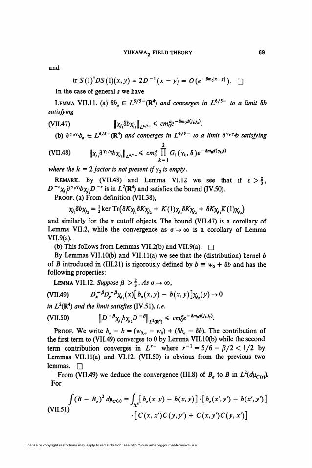
YUKAWA, FIELD THEORY 69
and
tTS(lfDS(l)(x,y) = 2D~x(x-y) = 0(e~Sm"\x-y\). Q
In the case of general s we have
Lemma VII.ll. (a) 8b„ E L6/5_(R4) and converges in L6'5' to a limit 8b
satisfying
(VII.47) IXÄJU*- < cmSe-Sm^^\
(b) 3Y»Y#0 E L6/5_(R4) and converges in L6/5~ to a limit 3Y"Y£ satisfying
2
(VII.48) HX^^X-JU- < cmS II G, (y„ S)*-*""^
where the k = 2 factor is not present ify2 is empty.
Remark. By (VII.48) and Lemma VI.12 we see that if e>§,
D -'xjV^ÛXjP -* is in L2(R4) and satisfies, the bound (IV.50).
Proof, (a) From definition (VII.38),
XÄ = 2-ker Tr(5^5^2 + * 0)XÄ2 + SK^K^j)
and similarly for the a cutoff objects. The bound (VII.47) is a corollary of
Lemma VII.2, while the convergence as o -» oo is a corollary of Lemma
VII.9(a).
(b) This follows from Lemmas VII.2(b) and VII.9(a). □
By Lemmas VII.10(b) and VII.11(a) we see that the (distribution) kernel b
of B introduced in (111.21) is rigorously defined by b = wn + 8b and has the
following properties:
Lemma VII. 12. Suppose ß > f. As a -> oo,
(VII.49) Dx-ßD-\(x)[ba(x,y) - b(x,y)]xJ1(y)-^0
in L2(R4) and the limit satisfies (IV.51), i.e.
(VII.50) \\D-%bx,D-b\\lHr4) < cmge-Sm^\
Proof. We write ba - b = (w0a - wQ) + (8ba - 8b). The contribution of
the first term to (VII.49) converges to 0 by Lemma VII.10(b) while the second
term contribution converges in U~ where r~x = 5/6 - ß/2 < 1/2 by
Lemmas Vll.ll(a) and VI.12. (VII.50) is obvious from the previous two
lemmas. □
From (VII.49) we deduce the convergence (III.8) of B„ to B in L2(dpC(s)).
For
f(B - Ba)2dpc,s)=[ \ba(x,y) - b(x,y)]-[b0(x',y') - b(x',y')]J JA4
(VII.51) . ..■[C(x,x')C(y,y')+C(x,y')C(y,x')]
License or copyright restrictions may apply to redistribution; see http://www.ams.org/journal-terms-of-use
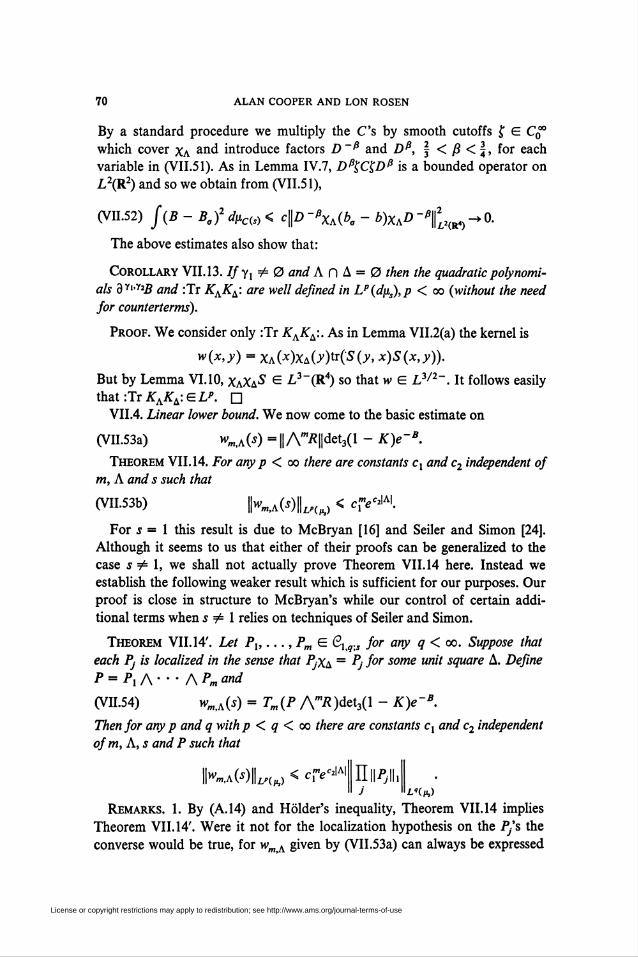
70 ALAN COOPER AND LON ROSEN
COBy a standard procedure we multiply the C's by smooth cutoffs f G C0°
which cover Xa anc* introduce factors D~B and Ds, \ < ß < \, for each
variable in (VII.51). As in Lemma IV.7, DBÇCÇDB is a bounded operator on
L2(R2) and so we obtain from (VII.51),
(VII.52) f(B - Ba? dpc(s) < c\\D -BXA(ba - b)XAD ̂¡|22(r4) -+ 0.
The above estimates also show that:
Corollary VII.13. Ifyx¥=0 and A n A = 0 then the quadratic polynomi-
als dy"y2B and :Tr KAKA: are well dejined in Lp(dps),p < oo (without the need
jor counterterms).
Proof. We consider only :Tr KAKA:. As in Lemma VII.2(a) the kernel is
w(x,y) = XA(x)xA(y)Hs(y> x)S(x,y)).
But by Lemma VI. 10, xAXAS E L3_(R4) so that w E L3/2~. It follows easily
thatíTrAV^GL'. DVII.4. Linear lower bound. We now come to the basic estimate on
(VII.53a) wm¡A(s) = || A"*||det3(l - K)e~B.
Theorem VII. 14. For any p < oo there are constants cx and c2 independent oj
m, A and s such that
(VII.53b) K,a(*)IU„) < &**.
For s = 1 this result is due to McBryan [16] and Seiler and Simon [24].
Although it seems to us that either of their proofs can be generalized to the
case í 7e 1, we shall not actually prove Theorem VII. 14 here. Instead we
establish the following weaker result which is sufficient for our purposes. Our
proof is close in structure to McBryan's while our control of certain addi-
tional terms when s =£ 1 relies on techniques of Seiler and Simon.
Theorem VII. 14'. Let Px,..., Pm G C,<q.s jor any q < oo. Suppose that
each Pj is localized in the sense that PjXA = Pj Jor some unit square A. Define
P = PXA'-- l\Pmand
(VII.54) wmA(s) = Tm(P AmR)^h(l - K)e~B.
Then for any p and q with p < q < oo there are constants cx and c2 independent
of m, A, s and P such that
IKaWIU,,, < c?e<MII IM
Remarks. 1. By (A. 14) and Holder's inequality, Theorem VII. 14 implies
Theorem VII.14'. Were it not for the localization hypothesis on the PJs the
converse would be true, for wmA given by (VII.53a) can always be expressed
License or copyright restrictions may apply to redistribution; see http://www.ams.org/journal-terms-of-use
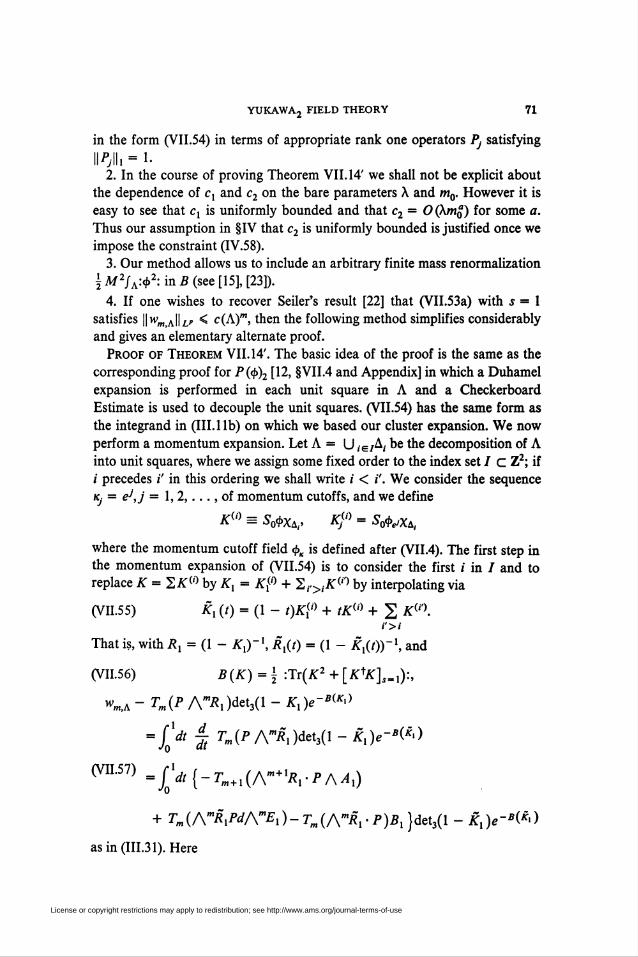
YUKAWA, FIELD THEORY 71
in the form (VII.54) in terms of appropriate rank one operators Py satisfying
llalli = I-2. In the course of proving Theorem VII. 14' we shall not be explicit about
the dependence of cx and c2 on the bare parameters X and m0. However it is
easy to see that cx is uniformly bounded and that c2 = 0(awjo) for some a.
Thus our assumption in §IV that c2 is uniformly bounded is justified once we
impose the constraint (IV.58).
3. Our method allows us to include an arbitrary finite mass renormalization
iM2/A:«i,2:in2?(see[15],[23]).
4. If one wishes to recover Seiler's result [22] that (VII.53a) with í = 1
satisfies ||wm aIL* < c(A)m, then the following method simplifies considerably
and gives an elementary alternate proof.
Proof of Theorem VII. 14'. The basic idea of the proof is the same as the
corresponding proof for P(<¡>)2 [12, §VII.4 and Appendix] in which a Duhamel
expansion is performed in each unit square in A and a Checkerboard
Estimate is used to decouple the unit squares. (VII.54) has the same form as
the integrand in (III.llb) on which we based our cluster expansion. We now
perform a momentum expansion. Let A = U ietA, be the decomposition of A
into unit squares, where we assign some fixed order to the index set / c Z2; if
/ precedes i' in this ordering we shall write i < i'. We consider the sequence
Kj = eJ,j = 1, 2,..., of momentum cutoffs, and we define
K(0 = S0<í>xA¡, Kj* = StfíVXA,
where the momentum cutoff field $K is defined after (VII.4). The first step in
the momentum expansion of (VII.54) is to consider the first i in / and to
replace K = 2 A» by Kx = Kx® + 2(>1A<''> by interpolating via
(VII.55) Kx (t) = (1 - t)K¡° + tKli) + 2 A(,'>.
That is, with Rx = (1 - A,)"1, Rx(t) = (1 - Kx(t)yx, and
(VH.56) B(K) = \ :Tr(A2 + [A+A],.,):,
wm,A - Tm(P Ami?,)det3(l - Kx)e~B^
-Jf* | Tm(P A"*i)det3(l - A5, )*"*(*)
(Vn.57) =S^dt[-Tm+x{Am+%-P/\Ax)
+ Tm(AmR,PdAmEx)- Tm(AmR, ■ P)BX }det3(l - Kx )e~B^)
asin(IIL31). Here
License or copyright restrictions may apply to redistribution; see http://www.ams.org/journal-terms-of-use
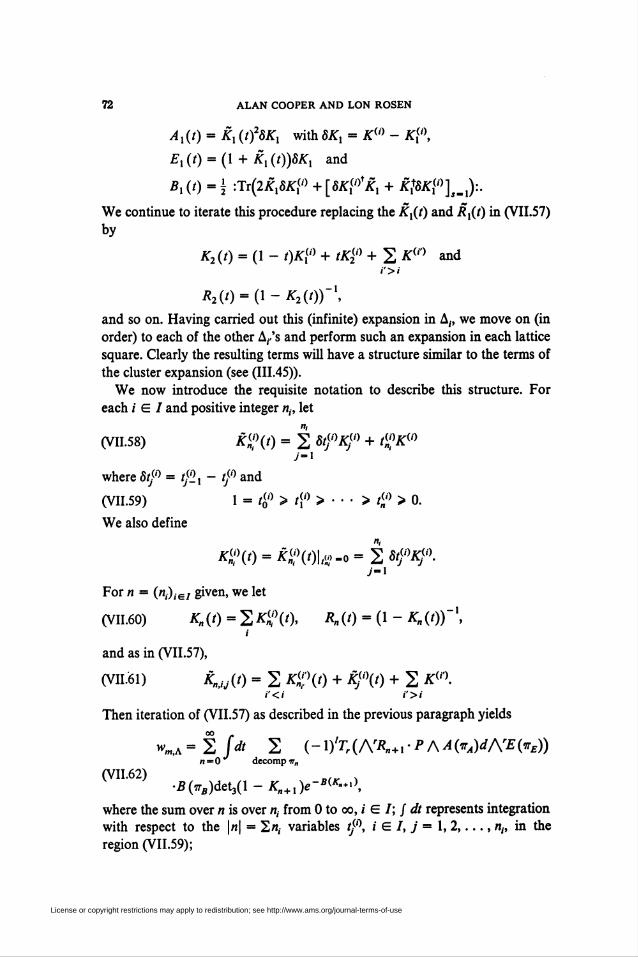
72 ALAN COOPER AND LON ROSEN
Ax(t) = Kx (t)28Kx with 8KX = KU) - K¡'\
Ex(t) = (I + Kx(t))8Kx and
Bx(t) = {- :lx(2kx8KxU)+[8Kf Kx + ÜJaaCf°]#-|):.
We continue to iterate this procedure replacing the Kx(t) and Rx(t) in (VII.57)
by
tf2(f) = (l - ,)#<<> + rA-w + 2 ¿t01 and
/?,(/)- (1-^(0)"',
and so on. Having carried out this (infinite) expansion in A,-, we move on (in
order) to each of the other A/s and perform such an expansion in each lattice
square. Clearly the resulting terms will have a structure similar to the terms of
the cluster expansion (see (111.45)).
We now introduce the requisite notation to describe this structure. For
each i E / and positive integer «,, let
«i
(VII.58) jfW(|) . 2 tfpKJp + t$K(i)/-«
where St}1* = tj'2x - r/° and
(VII.59) 1 = 4° > 'i° > • • • > <£° > 0.
We also define
7 = 1
For n = («,),-e/ given, we let
(vii.60) *„(/) = 2<(0. *„(') = (i - a»«)-1.
and as in (VII.57),
(VII.61) KnJJ(t) = 2 ^(0 + K}<\t) + 2 AT(f)./'</ e>t
Then iteration of (VII.57) as described in the previous paragraph yields
>Va= 2 /<* 2 {-\)'Tr{/\Rn+fPAA(ttA)dArE(trE))n=0 decompw„
(V11-62) „r^ >•2?K)det3(l-*„+,)*-*<*»♦■>,
where the sum over n is over n¡ from 0 to co, i E I; f dt represents integration
with respect to the |n| = 2«,- variables f/°, i E V, y = 1, 2,..., n¡, in the
region (VII.59);
License or copyright restrictions may apply to redistribution; see http://www.ams.org/journal-terms-of-use
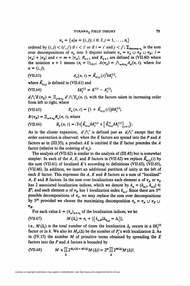
YUKAWA, FIELD THEORY 73
77„ = {a\a - (i,j); i E I,j = 1,..., «,}
ordered by (i,j) < (i',f) if i < i' or if i - i' and 7 < /; 2decompffji is the sum
over decompositions of irn into 3 disjoint subsets it„ = trA U irE U itB; I =
\itA\ + \itB\ and r = m + \itA\; Rn+X and Kn+X axe defined in (VII.60) where
the notation n + 1 means (n, + 1)(6/; A(irA) = Aae»/4«^"» 0» where for
a = (hf),
(VII.63) Aa(n,t) = Knt¡J(t)28K¡¡\
where A„ „ is defined in (VII .61) and
(VII.64) «A?0 = A(,) - Kj°;
dArE(irE) - n„e„£ d'ArEa(n, f), with the factors taken in increasing order
from left to right, where
(VII.65) Ea(n,t) = il+ knJJ(t))8K}i\
fiW = n„E,A(».')> where
(VII.66) 2?a(«, /) =:Tx(KntU8K^+[¿1,8^1^):.
As in the cluster expansion, d'/\f is defined just as dAr except that the
order convention is observed: when the E factors are spread into the P and A
factors as in (111.35), a product AE is omitted if the E factor precedes the A
factor (relative to the ordering of tt„).
The analysis of (VII.62) is similar to the analysis of (111.45) but is somewhat
simpler: In each of the A, E, and B factors in (VII.62) we replace KniJ(t) by
the sum (VII.61) of localized A's according to definitions (VII.63), (VII.65),
(VII.66). In addition, we insert an additional partition of unity at the left of
each E factor. This expresses the A, E and B factors as a sum of "localized"
A, E and B factors. In the sum over localizations each element a of 77,, or itE
has 2 associated localization indices, which we denote by ka • (fca,, ka2) E
Z4, and each element « of itB has 1 localization index kaX. Since there are 3'"'
possible decompositions of 77„, we may replace the sum over decompositions
by 3|n| provided we choose the maximizing decomposition 77n = tt¿ u ite U
itB.
For each value k = (ka)aB„ of the localization indices, we let
(VII.67) M (A,) = n, + \{ka,ß\AKß = A,.}|,
i.e., M (A,) is the total number of times the localization A7 occurs in a SK^
factor or in k. We also let MP(A) be the number of PJs with localization A. As
in (IV.15) the number M of primitive terms obtained by spreading the E
factors into the P and A factors is bounded by
(VII.68) M <n2"'(A)+Am)M(A)! = 2mIl2w(A)A/(A)!.A A
License or copyright restrictions may apply to redistribution; see http://www.ams.org/journal-terms-of-use
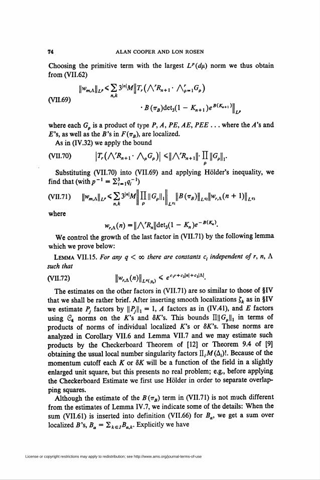
74 ALAN COOPER AND LON ROSEN
Choosing the primitive term with the largest Lp(dp) norm we thus obtain
from (VII.62)
IKAlL^-'Ml^A^+r Ap_i<?p)
>B(vB)det3(l-Kn+x)eB«'+>\
(VII.69) ",k
where each Gp is a product of type P, A, PE, AE, PEE ... where the A's and
E's, as well as the 5's in F(trB), are localized.
As in (IV.32) we apply the bound
(vii.70) \Tr(ArRn+r Apgp)\ <«A^+1||-n||Gp|1.p
Substituting (VII.70) into (VII.69) and applying Holder's inequality, we
find that(withp_1 = 23=1t7f')
(vii.71) |ka||l,<23wa/ HiiGpii, m«B)L«HA" + OIL«,n,k 9 ¿«i
where
^A(«)=«AX||det3(l-^)e-^.>.
We control the growth of the last factor in (VIL71) by the following lemma
which we prove below:
Lemma VII. 15. For any q < oo there are constants c¡ independent of r, n, A
such that
(VII.72) KaOOL«*) < e'"-+^"+^Al.
The estimates on the other factors in (VII.71) are so similar to those of §IV
that we shall be rather brief. After inserting smooth localizations Çk as in §IV
we estimate Pj factors by \\Pj\\x = 1, A factors as in (IV.41), and E factors
using G4 norms on the K's and 8K's. This bounds II||Gp||, in terms of
products of norms of individual localized K's or 8K's. These norms are
analyzed in Corollary VII.6 and Lemma VII.7 and we may estimate such
products by the Checkerboard Theorem of [12] or Theorem 9.4 of [9]
obtaining the usual local number singularity factors II,M (A,)!. Because of the
momentum cutoff each K or 8K will be a function of the field in a slightly
enlarged unit square, but this presents no real problem; e.g., before applying
the Checkerboard Estimate we first use Holder in order to separate overlap-
ping squares.Although the estimate of the B(ttb) term in (VII.71) is not much different
from the estimates of Lemma IV.7, we indicate some of the details: When the
sum (VII.61) is inserted into definition (VII.66) for Ba, we get a sum over
localized B's, Ba = *2keIBa k. Explicitly we have
License or copyright restrictions may apply to redistribution; see http://www.ams.org/journal-terms-of-use
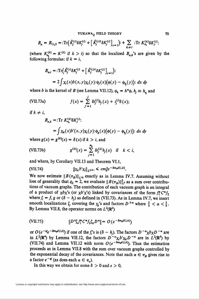
YUKAWAj FIELD THEORY 75
Ba = B,,J)=:Tx(K}»8K}»+[K}i»8K}»l_i):+ 2 :Tr A<«5AJ'>:k=£i
(where Kj& = K(k) if k > i) so that the localized BaJe's axe given by the
following formulas: if k = i,
Ba¡, -:Tt(KJ°ÔK}0 +[K}'n8KJ°]sml):
= ^Jxi{x)b(x,y)x,(y):<t>/(x)(<t>(y) - <f>hj(y)): dx dy
where b is the kernel of B (see Lemma VII.12), $h = h*$, h} = h and
j(VII.73a) fix) = 2 Stj%,(x) + fd(x);
/-iiik^i,
BaJc=:TxK^SK^:
= jxk(x)b'(x,y)X¡(y):<t>g(x)(<í>(y) - 4>hj(y)): dx dy
where g(x) = gw(x) = 8(x)ifk > i, and
"*(VII.73b) ga)(x) = 2 8tjk)hj(x) ii k< i,
j-i
and where, by Corollary VII.13 and Theorem VI.l,
(VTI.74) IM'xILv^ c<e-^('-.«.
We now estimate \\B(irB)\\Ln exactly as in Lemma IV.7. Assuming without
loss of generality that q2 = 2, we evaluate H-SO^Ill* as a sum over contribu-
tions of vacuum graphs. The contribution of each vacuum graph is an integral
of a product of x&x's (or Xb'x's) linked by covariances of the ioxmffC^
where ̂ = fig ox (8 - hj) as defined in (VII.73). As in Lemma IV.7, we insert
smooth localizations f, covering the x/s and factors D±a where § < a < f.
By Lemma VII.8, the operator norms on L2(R2)
(VII.75) |P %/f C*f2$kDa\\ = O (e-*M<U))
or 0(e-tJe-Sm°d«-ky) if one of them's is (5 - hjp The factors D ~axbxD ~a axe
in L2(R4) by Lemma VII.12, the factors D-ax¡b'XkD~a are in L2(R4) by
(VII.74) and Lemma VII.12 with norm 0(e~Sm<>d(i-k)). Thus the estimation
proceeds as in Lemma VII.8 with the sum over vacuum graphs controlled by
the exponential decay of the covariances. Note that each a EitB gives rise to
a factor e~w (as does each a E irn).
In this way we obtain for some 5 > 0 and e > 0,
License or copyright restrictions may apply to redistribution; see http://www.ams.org/journal-terms-of-use
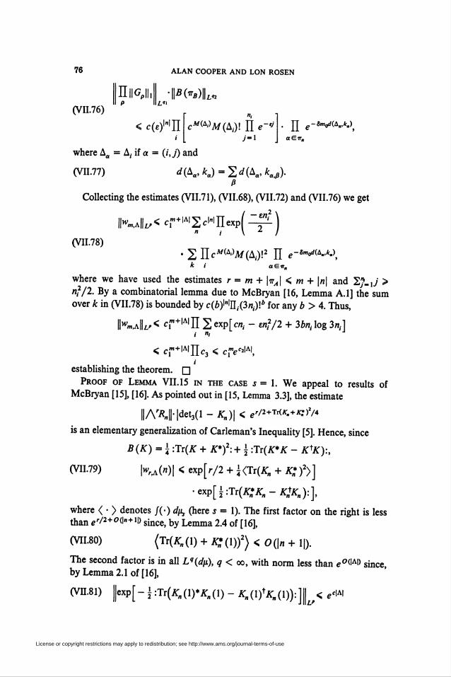
76
(VII.76)L">
niiGPn,p
< c(ef]l
ALAN COOPER AND LON ROSEN
cM^M^y. II e-*y-1
[ e-Sm0rf(Aa>fco))
where A0 = A, if a = (i,j) and
(Vll.ll) d(Aa,ka)=^d{Aa,kaS).ß
Collecting the estimates (VII.71), (VII.68), (VII.72) and (VII.76) we get
IK,a|L,< cr+|A|2c|n|IIexpi^i-j
• 2 üc^^MíA,)!2 II e-Sm^-k-\(VII.78)
aeir.
where we have used the estimates r = m + \tta\ < m + \n\ and 2/Li/ >
nf/2. By a combinatorial lemma due to McBryan [16, Lemma A.l] the sum
over k in (VII.78) is bounded by c(b)^Ui(3ni)lb for any b > 4. Thus,
IKa|L,< cr|A|n2exp[c«,. - e«2/2 + 3bn,log3«,.]í "/
< c,m+|A|Iïc3 < c¡V*|A|,i
establishing the theorem. □
Proof of Lemma VII. 15 in the case í = 1. We appeal to results of
McBryan [15], [16]. As pointed out in [15, Lemma 3.3], the estimate
||A'/y-|detj(l - K„)\ < em+W.+K?,*
is an elementary generalization of Carleman's Inequality [5]. Hence, since
B (K) - i :Tï(K + K*)2: + \ :1r(K*K - KyK):,
(VII.79) \wr¡A(n)\ < exp[r/2 + \<Jt(K„ + K* )2>]
■exp[±:TT(KZKn-Ktt%y-],
where < • > denotes /(•) dp, (here s = 1). The first factor on the right is lessthan e'ß+o{\n+i\) since; by Lemma 2.4 of [16],
(VII.80) (TriAO) + K*n(l)f) <0(\n+ 1|).
The second factor is in all Lq(dp), q < oo, with norm less than e°W) since,by Lemma 2.1 of [16],
(VII.81) \exp[-\:lT{Kn(l)*Kn(l) - Kn(l?Kn(l)):]\L< e™
License or copyright restrictions may apply to redistribution; see http://www.ams.org/journal-terms-of-use
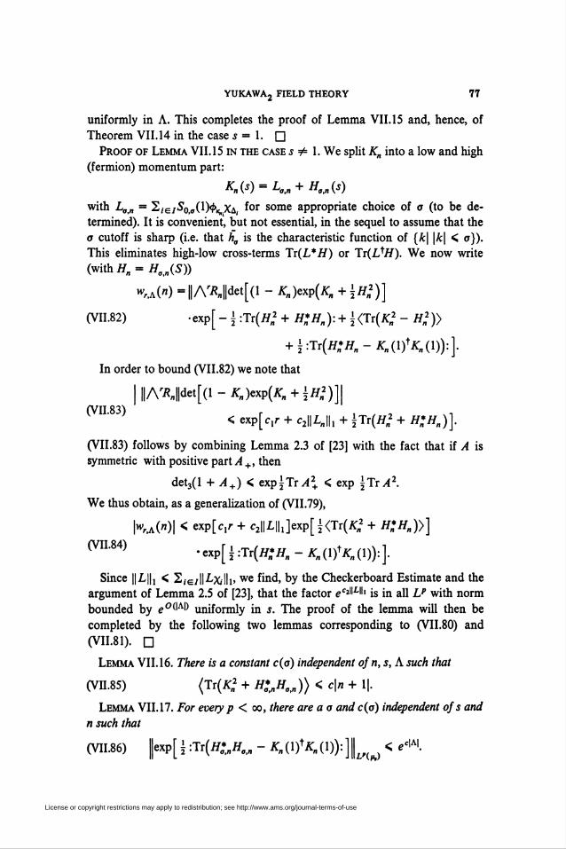
YUKAWAj FIELD THEORY 77
uniformly in A. This completes the proof of Lemma VII. 15 and, hence, of
Theorem VII. 14 in the case s = 1. □
Proof of Lemma VI 1.15 in the case j^ 1. We split Kn into a low and high
(fermion) momentum part:
Kn(s) = La,n + Ha,n(s)
with L0„ = Sye/S'o.oO^XA, f°r some appropriate choice of o (to be de-
termined). It is convenient, but not essential, in the sequel to assume that the
o cutoff is sharp (i.e. that h\ is the characteristic function of [k\ \k\ < o}).
This eliminates high-low cross-terms Tx(L*H) or Tx(L^H). We now write
(withi/n = //0>n(5))
«**<*) -||A'Äjdet[(l - A-n)exp(Afl + \H2)]
(VII.82) .exp[-\:TxiH2 + H*Hn): + \{JxiK2 - H2))
+ x2:lx(H:Hn- Kn(l)^Kn(l)):\
In order to bound (VII.82) we note that
\\\ArRn\\àet[(l-Kn)exp(Kn + \H2)]\
(VH.83) r . , , m< exp[c,r + callan, + \TxiH2 + //„*#„)].
(VII.83) follows by combining Lemma 2.3 of [23] with the fact that if A is
symmetric with positive part A +, then
det3(l + A+) < expjTxA2. < exp ±Tr,42.
We thus obtain, as a generalization of (VII.79),
|uv>A(«)| < exp[c,r + c2||L||I]exp[i<Tr(A'fl2 + /£//„)>]
(VIL84) .exp[i:Tr(^i/„-An(l)tAn(l)):].
Since ||L||, < 2/s/||LXilli» we fmd» by the Checkerboard Estimate and the
argument of Lemma 2.5 of [23], that the factor eClWU is in all Lp with norm
bounded by e°W) uniformly in s. The proof of the lemma will then be
completed by the following two lemmas corresponding to (VII.80) and
(VII.81). □
Lemma VII. 16. There is a constant c(o) independent ofn, s, A such that
(VII.85) (Tr(A2 + H^flJ)) < c\n + 1|.
Lemma VII.17. For every p < oo, there are a o and c(o) independent of s and
n such that
(VII.86) ¡exp[^:Tx(HlnHa¡n - Mtf^O)):]^ < e°W-
License or copyright restrictions may apply to redistribution; see http://www.ams.org/journal-terms-of-use
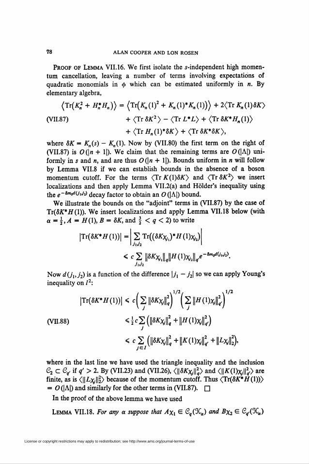
78 ALAN COOPER AND LON ROSEN
Proof of Lemma VII. 16. We first isolate the ¿-independent high momen-
tum cancellation, leaving a number of terms involving expectations of
quadratic monomials in <i> which can be estimated uniformly in n. By
elementary algebra,
(Tt(K2 + H*nHn)) = (Tr(*-„(1)2 + Kn(l)* Kn(l))) + 2<Tr Kn(l)8K}
(VII.87) + <Tr 8K2> - <Tr L*V) + <Tr 8K*Hn(l))
+ <Tr Hn(l)*8K) + <Tr 8K*8K),
where 8K = Kn(s) - Kn(l). Now by (VII.80) the first term on the right of
(VII.87) is 0(|n + 1|). We claim that the remaining terms are 0(|A|) uni-
formly in s and n, and are thus 0(\n + 1|). Bounds uniform in n will follow
by Lemma VII.8 if we can establish bounds in the absence of a boson
momentum cutoff. For the terms <Tr K(l)8K) and <Tr 8K2} we insert
localizations and then apply Lemma VII.2(a) and Holder's inequality using
the e~Sm^<JiJi> decay factor to obtain an O (|A|) bound.
We illustrate the bounds on the "adjoint" terms in (VH.87) by the case of
Tr(8K*H(l)). We insert localizations and apply Lemma VII.18 below (with
a = x2,A = H(l), B - 8K, and § < q < 2) to write
\Tr(8K*H(l))\ - 2Tr((SKx.)*tf(l)x,)JiJi i
<c2|Fx,1|J^(i)x,2||/-im^).Juh
Now d(jx,j2) is a function of the difference |y. - y'2| so we can apply Young's
inequality on I2:
\Tr{8K*H(l))\ < c(2 ||5^«2?) (2 ¡^(l)^)
(vn.88) <^2(i^l2f + ||Ä(i)^t)j
<^2(||^«2í+||ír(i^l2,+fiL^),ye/
where in the last line we have used the triangle inequality and the inclusion
S, c eq. if q' > 2. By (VII.23) and (VII.26), qSK^} and {\\K(l)XjW2^ arefinite, as is <||.Lxy|l2> because of the momentum cutoff. Thus (Tt(8K* H (I))}
= O (|A|) and similarly for the other terms in (VII.87). □
In the proof of the above lemma we have used
Lemma VII.18. For any a suppose that Axi E Qq(%a) and Bx2 E dy(3Ca)
License or copyright restrictions may apply to redistribution; see http://www.ams.org/journal-terms-of-use
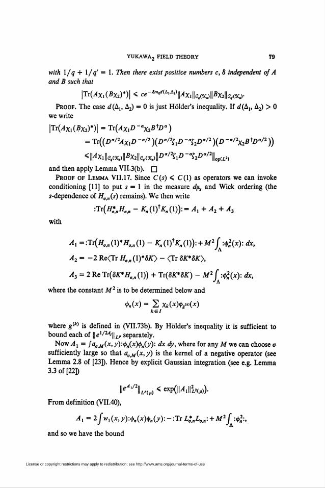
YUKAWAj FIELD THEORY 79
with l/q + l/q' = 1. Then there exist positive numbers c, 8 independent of A
and B such that
\Tt(AXi(BX2)*)\ < ce-Sm^^\\Axx\\e,(%J\Bx2\\e^-
Proof. The case </(A„ A^ = 0 is just Holder's inequality. If d(Ax, A2)>0
we write
|Tr(^Xi(5x2)*)| = Tr(AXlD-aX2ByDa)
= TT((Da/2AXlD ~a'2 )(D"/2ÇXD -%2Dtt'2 )(D -«l2X2ByDa'2 ))
<Hx1||e,wFX2||e,W«Z)a/2^Z)"a^o/2«opa2)
and then apply Lemma VII.3(b). □
Proof of Lemma VII.17. Since C(s) < C(l) as operators we can invoke
conditioning [11] to put s = 1 in the measure dp, and Wick ordering (the
¿-dependence of Ha„(s) remains). We then write
:Tt(H*nHa¡n - Kn(lj*Kn(l)):=Ax +A2 + A3
with
Ax = :Tr(Ha,n(l)*H0,n(l) - Kn(l?Kn(l)): + M2( :<b2(x): dx,•'A
A2 = -2 Re<Tr H„t„(l)*8K) - <Tr 8K*8K),
A3 = 2ReTT(8K*Hon(l)) + Tr(8K*8K) - M2 f :tf(x): dx,•'A
where the constant M2 is to be determined below and
<S>n(x) - 2 x«(*)fy»(*)kel
where g{k) is defined in (VII.73b). By Holder's inequality it is sufficient to
bound each of ||e1/'2'4-'||i>, separately.
Now A, = faaM(x, y)'-<i>„(x)<t>n(y): dx dy, where for any M we can choose a
sufficiently large so that aoM(x,y) is the kernel of a negative operator (see
Lemma 2.8 of [23]). Hence by explicit Gaussian integration (see e.g. Lemma
3.3 of [22])
II^IU,) < «P(lMtHk,))-From definition (VII.40),
Ax = 2fwx(x,y):<bn(x)<ba(y):-:TTLlnLay. + M2f^2:,
and so we have the bound
License or copyright restrictions may apply to redistribution; see http://www.ams.org/journal-terms-of-use
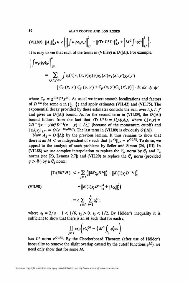
80 ALAN COOPER AND LON ROSEN
(VII.89) \\AX\\2L2< c\ fwx:<¡>n<pn: +||:Tr L*L: fL> + ¡M2f :<t>2:\\ \.[\\J L1 II J Wo)
It is easy to see that each of the terms in (VII.89) is O (|A|). For example,
il c II2Ik ii l2
= 2 ÍXi(x)wx(x,y)xj(y)Xr(x')wx(x',y')x/(y')ij.i'J' t= I
■ [C„.(x, x') Cjj. (y,y') + C,f (x,y')Cej(x\y)]-dx dx' dy dy'
where C,r = g(,)*C*g(0. As usual we insert smooth localizations and factors
of D ±tt for some a in (£, f ) and apply estimates (VII.42) and (VII.75). The
exponential decay provided by these estimates controls the sum over i,j, i',j'
and gives an 0(|A|) bound. As for the second term in (VII.89), the 0(|A|)
bound follows from the fact that :Tr L*L:= //„:<#>„<#>„:, where lg(x,y) =
2D~x(x - y)h*D~x(x - y) E LXo^ (because of the momentum cutoff) and
ÏÏXiloXjWo- m 0(e-Sm^ij\ The last term in (VII.89) is obviously 0(|A|).
Now A2 = 0(|A|) by the previous lemma. It thus remains to show that
there is an M < oo independent of s such that He^H^ = e0^. To do so, we
appeal to the analysis of such problems by Seiler and Simon [24, §111]. In
(VII.88) we use complex interpolation to replace the ß?. norm by Q^ and C4
norms (see [23, Lemma 2.7]) and (VII.29) to replace the ßq norm (provided
q > y)by a 0^ norm:
\Tx(SK*H)\ < c 2 {\\8KxjD'f2 +||A(l)x,Z>-«>||2ye/
(vi« +II*O)a>0í;+|i*||2:)
= <2 2a>(,),JSI i-l
where ex = 2/q - 1 < 1/6, e2 > 0, e3 < 1/2. By Holder's inequality it is
sufficient to show that there is an M such that for each /,
n exP(c^'> - \M2 ( :&:)
has Lp norm e0^. By the Checkerboard Theorem (after use of Holder's
inequality to remove the slight overlap caused by the cutoff functions gw), we
need only show that for some M,
License or copyright restrictions may apply to redistribution; see http://www.ams.org/journal-terms-of-use
YUKAWA2 FIELD THEORY 81
< 00.exp(x^-íM2j^goy.\\
According to the method of [24] this will be the case if for some M
(VII.91) f(XJ°)2dvMj<e-2,
where dvMJ is the Gaussian measure on S ' with mean zero and covariance
C(l + M2XjC)~x. (We may drop the ultraviolet cutoff g01 in the proof of
(VII.91).) The cases i = 2, 3, 4 of (VII.91) are dealt with in [24] and the case
/ = 1 is similar since we know that the kernel of Xj^ = \\8KxjDe,\\l is
pointwise bounded by an ¿-independent function in LPa~ (see Lemma VII.l).
DVII.5. Decoupling at s = 0. We now complete the proof of Lemma III.l by
verifying (111.15); i.e., if s = 0 on % c (Z2)* with R2~ % = \JX, a dis-
joint union, then in L2(dpC(s)),
(VII.92) B(A,s) = 2,B(A„s)i
where A, = A n X,. To prove (VII.92) we must show that the cross-terms
between different A/s vanish:
(VII.93) j:<l>(x)xAl(x)b(s; x,y)xAj(y)<t>(y): dx dy = 0
in L2(íz/xC(í)) if i i= j. If we estimate the L2(dpc^s)) norm of (VII.93) as in
(VII.52), we see that (VII.93) follows from the assertion that D ~pX\bX2D ~ß
— 0 in L2(R4) for some ß < \ where Xi = Xa and X2 = Xa • Tl"s m turn
follows if for any jx,j2 E S (R2),
(VII.94) fjx (x)Xx(x)b(s; x,y)X2(y)J2(y) dx dy = 0.
Suppose first that d s dist(supp/, u sup/2, ®0) > 0. Then if o > (2d)~x
we claim that Jx(x)xx(x)ba(s; x,y)x2(y)J2(y) = 0. For consider formula
(VII.41a) for b„ = b0a. Certainly 8(x — y) vanishes, as does S0a(s; x,y),
since S0(s; x,y) = 0 if x E A„y G A; and convolution with ha (see (III.9))
"blurs" the support of S0 by a distance of only l/2o. By the convergence
(VII.49) of ba to b as a -> 00 we thus deduce (VII.94) in the case d > 0.
When d = 0 we simply approximate j, by f,(n) with d > 0 such that, as
n -» 00, ftn)^>f, in both Lp, any p < 00, and in %ß for some ß > 0. Then
Xif¡w^X¡Ji in L> and in %a for a < Min(l, ß)/2 (by Lemma VH.3(c)).
Since b can be written as a sum b = w0+ 8b0 where w0D ~" defines a
bounded operator on L2(R2) and 8b0 G ¿/¿/11_ (see Lemma VII.12), we
conclude that
íñn)Xxbx1fin)-*¡JxXybX2J2
License or copyright restrictions may apply to redistribution; see http://www.ams.org/journal-terms-of-use
82 ALAN COOPER AND LON ROSEN
and this establishes (VII.94) and the decoupling (VII.92).
VII.6. Boson functional derivatives. In [4] Dimock and Glimm proved the
"integration by parts" formula
(VII.95) A fF(s, <f>) dpcU) = /( JL + I ^ . A,)f ̂ w
for a large class of functions F of the field cj> (actually their F's did not have
an explicit s dependence). Their method consists essentially of two parts. First
they show that (VII.95) holds if F is a cylinder function of the form
F(<b) = F(<t>(fx),..., <¡>(fn)) for some fixed/,, ...,/,£§ and polynomially
bounded function F in C2(R"). This is proved by explicit Gaussian integra-
tion and integration by parts. In this case the functional derivative 8/8<j> is
defined by
(VII.96) (g^)F)(*) -2 /,(*)3^(<K/i)- ••*(/»))
where 3, denotes the partial derivative with respect to the Ah variable. Then
for the family of functions F of interest they construct an approximating
sequence of cylinder functions [FN) such that as JV-» oo the integrals with
respect to dp, of FN, dFN/dsb, and (dC/dsb) ■ A^FN converge to the integrals
of F, dF/dsb and (dC/dsb) • A^F, respectively. The validity of (VII.95) for Fthen follows by the elementary
Lemma VII. 19. ///„ E C'([0, 1]), /„ ->/ and f'n-*g uniformly as n -> oo,
thenfeCx([Q,l])andf' = g.
We have applied formula (VII.95) to the functions F(s, <£) = rm(G) (see
(111.32)), where the «-derivatives are computed by the rules (111.24)—(111.26)
and the ^-derivatives are computed similarly just as if <b were a single variable
provided that we define
(VII.97) 8H(<b)/8<i>(y) = H(8y)
for linear functions H of </> (e.g. H =dyK). Of course, the functions F =
rm(G) are not specifically covered by the results of Dimock and Glimm and
in this subsection we verify (VII.95) for such F by following their procedure.
However, we wish to emphasize that we do not claim to be rigorously
justifying partial calculations such as (111.25). Rather, it is always necessary to
collect terms as in (111.31) and (111.33) so that R = (1 — K)~x occurs in a
single factor of the form A^- P°r formulas like (111.24)—(ÏII.27) do not even
make sense if 1 £ a(K). However after collecting terms we can assert:
Lemma VII.20. Let K be a (¿¡-valued continuously differentiable function of s
in an interval I c R, i.e. K E CX(I, Q2(%)), P E CX(I, ex(A"K)), B E
License or copyright restrictions may apply to redistribution; see http://www.ams.org/journal-terms-of-use
YUKAWA2 FIELD THEORY 83
CX(I), and t„(P) be as in (111.32). Then t„(P) is dijjerentiable in I and
(III.33a) holds.
Proof. The formulae (111.25), (111.26), (111.27) and so (III.33a) certainly
hold for all s such that 1 G o(K(s)) (see for example [5]). If 1 G o(K(s)) then
there is an 6 > 0 such that 1 g o(XK(s)) for 0 < |X - 1| < e. So (III.33a)
holds for K replaced by XK in the definition of rn(P). But the right-hand side
of (III.33a) is continuous in X by results of the Appendix of [23]. Thus by
Lemma VII.19, (III.33a) does indeed hold at X - 1 even if 1 G o(K(s)). □
We define cylinder function approximants to K(<$>) so as to preserve the
algebraic structure of the expressions involved. First we apply boson and
fermion momentum cutoffs, approximating K(<j>) by KaK((¡>) (see (VII.4))
which is in Qx(%) for all <i> G S'. Let rmaK(G) denote the corresponding
cutoff version of rm(G). Then for the arguments G of im which occur in the
derivative formula (111.33), we know thatjrm „ K(G) dps-* ¡Tm(G) dp,. This
follows by a dominated convergence type argument as in the proof of
Theorem IV.l, since by the estimates of the preceding subsections Tm>0ilt(G) G
Lp(dps) for any p < oo, uniformly in o and k. By Lemma VII.19 it thus
suffices to prove (VII.95) for KgK. We henceforth fix o and k which will be
suppressed in the notation.
Next, we choose an orthonormal basis {e,} in %x/2 and approximate
K* = A or At by the finite rank operators
(VII.98) K* if) = ENK* (<¡>)EN - 2 e,(e„ K# (*),-,)(* • )iJ<N
with matrix elements
(VII.99) CW.-lf'''*'*'-**) »"<*[0 Hioxj > N,
where kt =kßand
kij{y) =// dx e,(x)DS0,a(x, z)xA(z)ej(z)hK(z - y) dz
(VII. 100)
-*(*)r
Letting FN be the approximant to F obtained by replacing K by KN we
verify (111.33) by means of Lemma VII.20. In this connection, note that the
definition (VII.96) of 8FN/8<$>(x) does indeed coincide with the prescription
for calculating a 8/8$ derivative given in (VII.97). We illustrate this in the
simple case F = det3(l - A):
License or copyright restrictions may apply to redistribution; see http://www.ams.org/journal-terms-of-use
84 ALAN COOPER AND LON ROSEN
^y dctj(l - K(t)) = 2 k0(x) -±- det3(l - *(*)) (by (VII.96))
= 2K(8x)uK(<b)2^ g|-í:](«í>)det3(l - K(<b)) (by(VII.100))
= K(^2K(8x)i/uyet3(l-K(^))
= K(<b)2K(8x)det3(l - K(<b))
since Jy = dK/dKy has Im matrix element (J¡j)lm = 5,v5,m.
Since KaK EC. for all t> E S ', Â^ -» K in 6,, as AT -» oo, pointwise in <f>.
So if F(<f>) is of the form F(<b) = rm(G) as defined in (111.32), then FN -* F,
dFN/dsb -*dF/dsb, (dC/dSb) ■ A^FN -» (dC/dsb) ■ A^F pointwise in <b. Since
ll-^jvlli < llalli» tne EN, ̂ EN/dsb, and (3C/3í¿,) • ̂ Fn are dominated uni-formly by cxeCimi+m which is in Lx(dp,) so that by the dominated conver-
gence theorem, their integrals converge. This establishes (VII.95) for K =
Appendix. Antisymmetric tensor products. In this Appendix we collect and
prove those properties of fermi statistics that we have used throughout the
paper. We begin with some definitions. Given a separable Hilbert space %,
let A"3C be its «-fold antisymmetric tensor product. It is convenient to
regard A"^ as a subspace of the ordinary tensor product ®"%, and to
identify an operator/I on A"^ with me operator on ®"% which equals A
on A"3C and is zero on (A"^C)±. We let irn be the orthogonal projection in
<E>"3C onto A"3C- The antisymmetric tensor product of vectors ex,..., e„ £
% is
(A.1) ex A • • • A èn = mnex ® • • • 8 en = -Jr 2 sgn ae ® • • • 8 e .n] oes„
If {e¡} is an orthonormal basis for %, then {(n\)x^2e¡ A ' * * A ^} with
¡i < i2 < • ' • < i„ is an orthonormal basis for A"^- Note that
(A.2) (/, A • • • A/„, gi A • • • A &) - («! )_,«K/p*)
from which we obtain the basic identity (1.11). Given « (bounded) operators
Ax,..., An on %, their antisymmetric tensor product is defined on A"3C by
(A.3a) Ax A A2 A • • • A A„ = mnAx 8 • • • 8 ¿„v
Alternatively, .4, A • • ' A An may be defined by its action on a basis vector
(A.3b) (Ax A • • • A ¿„K A • • • A \ - ¿- 2 ^..«i, A • • • A Vv"• «es,
License or copyright restrictions may apply to redistribution; see http://www.ams.org/journal-terms-of-use
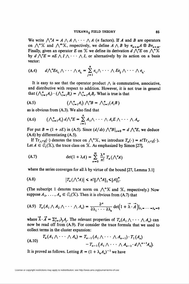
YUKAWAj FIELD THEORY 85
We write A"A =^A^A,,,A^(" factors). If A and B are operators
on An% and Am^> respectively, we define A f\ B by irn+mA ® Birn+n.
Finally, given an operator E on % we define its derivation d A"E on A"^
by d A"E = nE A IA ■ ■ • A L ox alternatively by its action on a basis
vector:
(A.4) dA"Ee,x A • • • A «(, - 2 %A • • • A Eei A • • • A \y"-i
It is easy to see that the operator product A is commutative, associative,
and distributive with respect to addition. However, it is not true in general
that i A". XA¡) • (A"-iB,) = A".\A¡Br What is true is that
(A.5) (AUA)AHB"A'!-l(AlB)
as is obvious from (A.3). We also find that
(A.6) (A?. A) dA"E - i AxA • • • A A,E A • • • A AH.i-l
For put B = (1 + sE) in (A.5). Since (d/ds) A"^L-o " d A"E, we deduce(A.6) by differentiating (A.5).
If TrA»5¿(.) denotes the trace on A"^> we introduce Tn(-) = n\TxAnyf-).
Let A E Gx(%), the trace class on %. As emphasized by Simon [27],
(A.7) det(l + X4) = 2 ^Tn(A"A)
where the series converges for all X by virtue of the bound [27, Lemma 3.1]
(A.8) |rn(A^)|<«!||A^||,<H|i;.
(The subscript 1 denotes trace norm on A"3C and %, respectively.) Now
suppose Ax,. .. ,AnE ßx(%). Then it is obvious from (A.7) that
(A.9) T„(AXAA2A--- AA„)= aA[ a" dKdet(l + X-A)\Xi.....K_0
where X-A = Sy-iA^-. The relevant properties of T„(AX A ' ' ' AA„) can
now be read off from (A.9). For consider the trace formula that we used to
collect terms in the cluster expansion:
T„(Al A • • • A An) = Tn_x iAxA--- /\An_x)-TxiAn)(A-10) , , %
-Tn.x{AxA--- AAn_x-dA"-XAn).
It is proved as follows. Letting R = (1 + X„An)~x we have
License or copyright restrictions may apply to redistribution; see http://www.ams.org/journal-terms-of-use
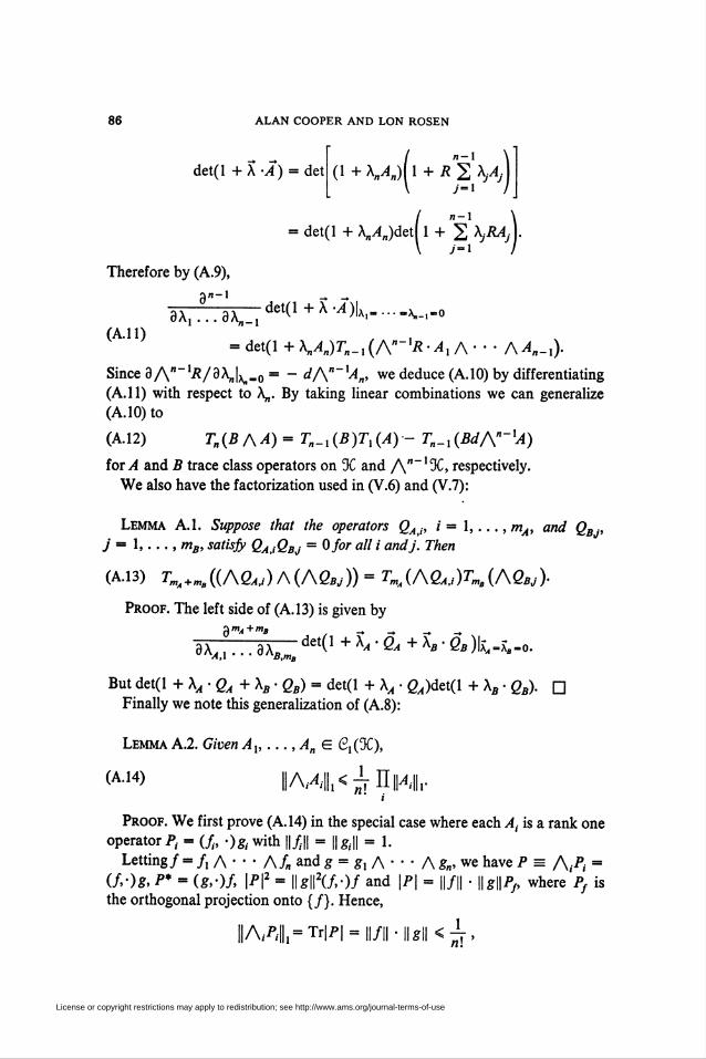
86 ALAN COOPER AND LON ROSEN
det(l +X -A) = det/ "-1 1
(1 + XnAn)[ 1 + i? 2 Vi\ 7 = 1 J
n-1
= det(l + V4„)detl 1 + 2 XjRAA.
Therefore by (A.9),
g«-I
9A,(All)
g^— det(l+A^)|Xi=...=Vi„0
= det(i + xn^)rn_1(An_IJR-^iA--- A4,-i).
Since 3An-1-R/3\,l\,-o = _ dA"~XAn, we deduce (A.10) by differentiating
(A. 11) with respect to A,,. By taking linear combinations we can generalize
(A.10) to
(A.12) T„(B /\A) = Tn_x(B)Tx(A)- Tn_x(BdA"-'A)
for A and B trace class operators on % and A"1^» respectively.
We also have the factorization used in (V.6) and (V.7):
Lemma A.l. Suppose that the operators QA¡, i = 1,..., mA, and QBJ,
j = 1,. .., mB, satisfy QAiQBJ = Ofor all i andj. Then
(A.13) T„A+mB((AQA,)A(AQbj)) = TmA(AQA,)Tms{AQBj)-
Proof. The left side of (A.13) is given by
dXAyX ... dxBmBdet(l+XA-QA+XB-QB)\tA=~XB=0.
But det(l + XA ■ QA + XB ■ QB) - det(l + XA ■ QA)det(l + XB ■ QB). D
Finally we note this generalization of (A.8):
Lemma A.2. Given A x, ..., An £ 6, (%),
(A.14) «A^ll,^ niNir
Proof. We first prove (A.14) in the special case where each A¡ is a rank one
operator P, = (/, -)&with ||/|| = ||g,|| = 1.
Letting/ = /, A • • • A/„ and g = gx A • • • A g„, we have P = A,P, =
(/V)S, P* = (*,-)/, \P\2 = IUH2(/,-)/ and \P\ = 11/11 • \\g\\Pf, where Pf isthe orthogonal projection onto {/}. Hence,
||A^4=Tr|P| = ||/||.||g||<-i-,
License or copyright restrictions may apply to redistribution; see http://www.ams.org/journal-terms-of-use
YUKAWA, FIELD THEORY 87
where in the last inequality we have used (A.2) and Hadamard's determinant
inequality [5]. But each A, has a canonical representation A, = 27a/AP1w,
with P,u"> a rank one operator of the above type, a^ > 0, and \\A,\\X = 2>fl//').
Therefore by the triangle inequality,
I A^|, < 2 oJW ... a^\\P^ A • • • A Wl
<±2aV...aP = ±TL\\A,\\v D
References
1. M. Abramowilz and I. A. Stegun (Editors), Handbook of mathematical fonctions, with
formulas, graphs, and mathematical tables, Nat. Bur. Standards Appl. Math. Ser., 55, U.S. Govt.
Printing Office, Washington, D.C., 1964. MR 29 #4914.2. D. Brydges, Cluster expansions for fermion fields by the time dependent Hamiltonian approach
(preprint).3. R. Courant and D. Hubert, Methods of mathematical physics. Vol. II, Interscience, New
York, 1962. MR 25 #4216.4. J. Dimock and J. Glimm, Measures on the Schwartz distribution space and applications to
PQfiifield theories, Advances in Math. 12 (1974), 58-83. MR 50 # 1665.5. N. Dunford and J. T. Schwartz, Linear operators. Part II, Interscience, New York, 1963.
MR 32 #6181.6. J. Feldman and K. Osterwalder, The Wightman axioms and the mass gap for weakly coupled
(<j>4)3 quantum field theories, Ann. Physics 97 (1976), 80-135.
7. J. Fröhlich, Schwinger functions and their generating functionals. I, Helv. Phys. Acta 47
(1974), 265.8. J. Glimm, A, Jaffe and T. Spencer, The particle structure of the weakly coupled P($h. model
and other applications of high temperature expansions. Part I: Physics of quantum field models,
Constructive Quantum Field Theory (G. Velo and A. Wightman, Editors), Springer-Verlag,
Berlin and New York, 1973, pp. 132-198.9. _, The particle structure of the weakly coupled P(<¡>)2 model and other applications of
high temperature expansions. Part II: The cluster expansion, Constructive Quantum Field Theory
(G. Velo and A. Wightman, Editors), Springer-Verlag, Berlin and New York, 1973, pp. 199-242.
10._, The Wightman axioms and particle structure in the %($)2 quantum field model, Ann.of Math. (2) 100 (1974), 585-632. MR 50 # 15694.
11. F. Guerra, L. Rosen and B. Simon, The Pifa Euclidean quantum field theory as classicalstatistical mechanics, Ann. of Math. (2) 101 (1975), 111-259.
12._, Boundary conditions for the P(«f>)2 Euclidean field theory, Ann. Inst. H. Poincaré A25 (1976), 231-334.
13. J. Magnen and R. Sénéor, The infinite volume limit of the <f>4 model, Ann. Inst. H. Poincaré(to appear).
, 14. _, 77ie Wightman axioms for the weakly coupled Yukawa model in two dimensions,Ecole Polytechnique (preprint).
15. O. McBryan, Finite mass renormalizations in the Euclidean Yukawa2 field theory, Comm.Math. Phys. 44 (1975), 237-243.
16. _, Volume dependence of Schwinger functions in the Yukawa2 field theory, Comm.Math. Phys. 45 (1975), 279-294.
17._, Contribution to Internat. Colloq. on Math. Methods of Quantum Field Theory,Marseille, 1975.
License or copyright restrictions may apply to redistribution; see http://www.ams.org/journal-terms-of-use
88 ALAN COOPER AND LON ROSEN
18. K. Osterwalder and R. Schrader, Euclidean Fermi fields and a Feynman-Kac formula for
boson-fermion models, Helv. Phys. Acta. 46 (1973/74), 277-302. MR 51 #2524.19. _, Axioms for Euclidean Green's functions. I, II, Comm. Math. Phys. 31 (1973),
83-112; ibid. 42 (1975), 281-305. MR 48#7834; 51 # 12189.20. M. Reed and B. Simon, Methods of modern mathematical physics. Vol. II: Fourier analysis,
self-adjointness. Academic Press, New York, 1975.
21. L. Rosen, Renormalization of the Hilbert space in the mass shift model, J. Mathematical
Phys. 13 (1972), 918-927. MR 45 #8176.22. E. Seiler, Schwinger functions for the Yukawa model in two dimensions with space-time cutoff,
Comm. Math. Phys. 42 (1975), 163-182. MR 51 # 12208.23. E. Seiler and B. Simon, On finite mass renormalizations in the two dimensional Yukawa
model, J. Mathematical Phys. 16 (1975), 2289-2293.24. _, Bounds in the Yukawa2 quantum field theory: Upper bound on the pressure,
Hamiltonian bound and linear lower bound, Comm. Math. Phys. 45 (1975), 99-114.25._, Nelson's symmetry and all that in the Yukawa2 and ($4)3 field theories, Ann. Physics
97 (1976), 470-518.26. B. Simon, The Pifo Euclidean (quantum) field theory, Princeton Univ. Press, Princeton,
N.J., 1974.27. _, Notes on infinite determinants of Hilbert space operators, Advances in Math (to
appear).
28. T. Spencer, The mass gap for the P(<p)2 quantum field model with a strong external field,
Comm. Math. Phys. 39 (1974), 63-76. MR 50 # 15732.29. E. M. Stein, Singular integrals and differentiability properties of functions, Princeton Univ.
Press, Princeton, N.J., 1970. MR 44 #7280.30. R. F. Streater and A. S. Wightman, PCT, spin and statistics and all that, Benjamin, New
York, 1964. MR 28 #4807.
Department of Mathematics, University of Toronto, Toronto, Ontario M5S 1A1,
Canada
Current address: Department of Mathematics, University of British Columbia, Vancouver,
British Columbia V6T 1W5, Canada
License or copyright restrictions may apply to redistribution; see http://www.ams.org/journal-terms-of-use