the weak job recovery in a macro model of search and ... · parameters, recruiting intensity may be...
TRANSCRIPT

FEDERAL RESERVE BANK OF SAN FRANCISCO
WORKING PAPER SERIES
The Weak Job Recovery in a Macro Model of Search and Recruiting Intensity
Sylvain Leduc
Bank of Canada
Zheng Liu Federal Reserve Bank of San Francisco
November 2017
Working Paper 2016-09
http://www.frbsf.org/economic-research/publications/working-papers/wp2016-09.pdf
Suggested citation:
Leduc, Sylvain, Zheng Liu. 2017. “The Weak Job Recovery in a Macro Model of Search and Recruiting Intensity.” Federal Reserve Bank of San Francisco Working Paper 2016-09. http://www.frbsf.org/economic-research/publications/working-papers/wp2016-09.pdf The views in this paper are solely the responsibility of the authors and should not be interpreted as reflecting the views of the Federal Reserve Bank of San Francisco or the Board of Governors of the Federal Reserve System.
THE WEAK JOB RECOVERY IN A MACRO MODEL OF SEARCH ANDRECRUITING INTENSITY
SYLVAIN LEDUC AND ZHENG LIU
Abstract. An estimated model with labor search frictions and endogenous variations in
search intensity and recruiting intensity does well in explaining the deep recession and weak
recovery of the U.S. labor market during and after the Great Recession. The model features
a sunk cost of vacancy creation, under which firms rely on adjusting both the number of
vacancies and recruiting intensity to respond to aggregate shocks. This stands in contrast
to the textbook model with free entry, which implies constant recruiting intensity. Our
estimation suggests that fluctuations in search and recruiting intensity driven by produc-
tivity and discount factor shocks help substantially bridge the gap between the actual and
model-predicted job filling and finding rates.
I. Introduction
The U.S. labor market has improved substantially since the Great Recession. The unem-
ployment rate has declined steadily from its peak of about 10 percent in 2009 to less than
4.5 percent in 2017, accompanied by a steady increase in the job openings rate. However,
the recovery of in hiring has been much more subdued in comparison.
These patterns present a puzzle for the standard labor search model. In the standard
model, hiring is related to unemployment and job vacancies through a matching func-
tion. The matching function implies that the job filling rate—defined as new hires per job
vacancy—is inversely related to labor market tightness measured by the vacancy-unemployment
Date: November 13, 2017.
Key words and phrases. Unemployment, vacancies, recruiting intensity, search intensity, costly vacancy
creation, weak job recovery, business cycles.
JEL classification: E32, J63, J64.
Leduc: Bank of Canada. Email: [email protected]. Liu: Federal Reserve Bank of San
Francisco. Email: [email protected]. We benefited from comments by Stefano Gnocchi, Bart Hobijn,
Marianna Kudlyak, Nicolas Petrosky-Nadeau and conference participants at the Third Annual Macroe-
conomics and Business CYCLE Conference at UC Santa Barbara, the Norges Bank’s workshop on New
Developments in Business Cycle Analysis: The Role of Labor Markets and International Linkages, and the
2016 Society for Economic Dynamics’s annual meeting. We also thank Andrew Tai for research assistance
and Anita Todd for editorial assistance. The views expressed herein are those of the authors and do not
necessarily reflect the views of the Bank of Canada, the Federal Reserve Bank of San Francisco, or the
Federal Reserve System.1
THE WEAK JOB RECOVERY 2
(v-u) ratio. It also implies that the job finding rate—defined as new job matches per unem-
ployed worker—is positively related to labor market tightness. Thus, when the vacancy rate
increases and the unemployment rate falls, as has been the case during the recent recovery,
the v-u ratio rises, pushing the job finding rate up and the job filling rate down.
The standard theory fails to predict the deep labor market downturn and the subsequent
weak job recovery. As shown in Figure 1, the theory’s predicted paths for the job filling
rate and the job finding rate tracked the data fairly well up to early 2009. Since then, the
theory-implied series both lie significantly above those observed in the data. The reason for
these discrepancies is that the actual hiring rate fell more during the Great Recession and,
during the recovery, it did not increase as much as predicted by the theory with the standard
matching function.1,2
To understand the forces behind this weak job recovery, we develop and estimate a DSGE
framework that incorporates endogenous variations in two additional margins of labor-market
adjustment: search intensity and recruiting intensity. We examine the quantitative impor-
tance of cyclical fluctuations in search and recruiting intensity for the job filling and finding
rates in our estimated general equilibrium model.
We make three contributions to the literature. First, we develop a DSGE model that allows
for endogenous variations in recruiting intensity because vacancy creation incurs a sunk
cost. In the textbook model with recruiting intensity (Pissarides, 2000), vacancy creation
1 The standard matching function takes the form mt = µuαt v1−αt , where mt denotes new job matches,
ut and vt denote unemployment and job vacancies, respectively, α measures the elasticity of matching with
respect to unemployment, and µ is a scale parameter that captures the average matching efficiency. With
this matching function, the job filling rate is given by qvt ≡ mt
vt= µ
(vtut
)−αand the job finding rate is given
by qut ≡ mt
ut= µ
(vtut
)1−α. The job filling and finding rates implied by the standard matching function shown
in Figure 1 are calculated by using the observed data on job openings (from JOLTS) and the unemployment
rate (from BLS), with α = 0.5. By construction, the job filling rate and the job finding rate implied by the
standard matching function are perfectly negatively correlated. To highlight the changes of the job filling
and finding rates implied by the model relative to those in the data, we transform each series into log units
and normalize each series by setting the first observation to zero (so that all subsequent observations are
log-deviations from the first observation). Under this normalization, the scale parameter µ in the matching
function becomes irrelevant.2Alternative measures of the job finding rate are also used in the literature. One such alternative is based
on the transition rate from unemployment to employment reported in the Current Population Survey (CPS).
This CPS measures is highly correlated with our measure, with a correlation of about 0.96 over the JOLTS
sample period from December 2000 to July 2017. Another measure of the job finding rate considered by
Shimer (2005) is calculated based on the level and duration of unemployment. However, the Shimer measure
is not well-suited for the post-2008 period because of large swings in the distribution of unemployment
duration (Rothstein, 2011; Elsby et al., 2011).
THE WEAK JOB RECOVERY 3
is costless (i.e., there is free entry). When macroeconomic conditions change, firms vary
the number of vacancies—which are costless to create or destroy—to meet new hiring needs
and choose the level of recruiting intensity to minimize the cost of posting each vacancy.
The free-entry assumption implies counterfactually that vacancies are a flow variable that
can be adjusted continuously. Furthermore, as shown by Pissarides (2000), free-entry also
implies that recruiting intensity is independent of macroeconomic fluctuations. However,
in our model where vacancy creation incurs a sunk cost, vacancies become a slow-moving
state variable, and firms adjust both the number of new vacancies and recruiting intensity
in response to aggregate shocks. Thus, our model generates not only plausible vacancy
dynamics, but also business-cycle variations in recruiting intensity.3
In our model, the cyclical properties of recruiting intensity are a priori ambiguous. Optimal
recruiting intensity results from a tradeoff between the marginal costs of recruiting efforts
and the marginal benefit of raising the probability of filling a job opening, thus obtaining
the net value of a filled position. Although by filling a position the firm gains the value
of an employment match, it also loses the value of an open vacancy, which is non-zero in
equilibrium because of costly entry. Because the match value and the vacancy value both
decline in a recession, the net value of filling a vacancy is ambiguous. Depending on model
parameters, recruiting intensity may be pro- or counter-cyclical.
Our second contribution is to quantitatively examine the importance of cyclical fluctua-
tions in search and recruiting intensity for the job filling and finding rates. We do so by
estimating the model using Bayesian methods, fitting three monthly time series data of the
U.S. labor market: the unemployment rate, the job vacancy rate, and a measure of search
intensity.
The model estimation shows that recruiting intensity is procyclical and positively corre-
lated with aggregate hiring; and it interacts with cyclical variations in search intensity to
amplify labor market dynamics. With sharp declines in both search intensity and recruiting
intensity during the Great Recession and with weak recoveries in these intensive margins fol-
lowing the recession, our model predicts a sharp downturn and weak recovery in hiring, and
thus much lower job filling and finding rates than those implied by the standard matching
function without these intensive margins. Furthermore, our model’s predicted recovery paths
of the job filling and finding rates are roughly in line with the data, as shown in Figure 2.
3We are not the first to introduce fixed costs of vacancy creation. Elsby et al. (2015) consider a labor
search model with fixed vacancy creation costs to examine the qualitative implications of recruiting intensity
for shifts in the Beveridge curve. Fujita and Ramey (2007) introduce a fixed cost of creating vacancies in a
search model to account for the sluggish responses of employment and the v-u ratio following productivity
shocks, although they do not model recruiting intensity. See Coles and Moghaddasi Kelishomi (2011) for a
detailed discussion of the implications of costly entry for the labor market dynamics.
THE WEAK JOB RECOVERY 4
Remarkably, the periods for which our DSGE model outperforms the standard model
coincide with those during which the predicted paths of the job filling and finding rates from
the standard matching function diverged from those in the data. In contrast, the standard
matching function does equally well as our DSGE model prior to the depth of the Great
Recession in 2009, as shown in Figure 2. The improvement in the fit of our model to the
data stems from fluctuations in the search and recruiting intensity. As Figure 3 shows, our
measure of search intensity is procyclical and falls sharply during the Great Recession. It
has rebounded sharply after the recession, but it has not fully recovered to the pre-recession
level. The sharp decline in search intensity during the Great Recession and its weak recovery
contributed to the sharp downturn in hiring in the recession and the subdued recovery. In
addition, shocks in our model that led to declines in search intensity also led to declines in
recruiting intensity, which further depress hiring, contribution to the weak job recovery.
In our estimated model, forecast error variance decompositions show that the labor market
dynamics are driven mainly by a technology shock and a discount factor shock, and to a
lesser extent, also by a job separation shock. As we discuss below, our estimated persistence
and volatility of these structural shocks are in line with the calibration in the literature, such
as the studies by Shimer (2005) and Hall (2017).
Our model shares the Shimer (2005) puzzle of the standard DMP model: unless real
wages are rigid, it is difficult to generate the observed large volatilities in unemployment
and vacancies. Unsurprisingly, with real wage rigidities assumed in our model, technology
shocks are an important source of labor market fluctuations. It is also unsurprising that
a job separation shock plays a relatively minor role in the model, because it generates
counterfactually positive correlations between unemployment and vacancies (Shimer, 2005).
What is new is that a discount factor shock plays a quantitatively important role in driving
labor market fluctuations, mainly through its impact on the present values of a job match
and an open vacancy for firms, and also on the employment surplus for job seekers. By
driving changes in these present values, a discount factor shock contributes to a significant
fluctuations in unemployment, vacancies, search and recruiting intensity, and hiring. This
finding is in line with the literature (Hall, 2017).4
Our third contribution is to show that, despite our macro approach, the aggregate cor-
relation between hiring and recruiting intensity obtained from our estimated DSGE model
is positive and relatively high, broadly in line with estimates derived from micro data. In
particular, Davis et al. (2013) construct a measure of recruiting intensity based on the Job
4Albuquerque et al. (2016) argue that discount factor shocks are important for asset pricing models
because they give rise to a valuation risk that allows the model to account for the volatile asset price
fluctuations and the weak correlations between stock returns and fundamentals.
THE WEAK JOB RECOVERY 5
Openings and Labor Turnover Survey (JOLTS) at the establishment level. They present
evidence that employers rely not only on the number of vacancies, but also heavily on other
instruments for hiring, which they call recruiting intensity. Under the assumption that their
microeconomic estimates hold at the macro level, Davis et al. (2013) document a strong
correlation between recruiting intensity and hiring at the aggregate level. Our work comple-
ments theirs by providing a macro perspective on the positive relationship between recruiting
intensity and hiring.
Despite a better fit to the data along several important dimensions, our model has several
shortcomings. First, our model misses the timing of the trough in hiring during the Great
Recession by about one year, although the depth of the predicted fall is roughly in line with
that observed in the data. This lagged response is partly driven by the persistent declines in
search intensity and recruiting intensity during the downturn. Second, we emphasize that the
model’s improved performance is partly driven by the procyclicality of the search intensity
measure that we use in estimating the model. When we estimate the model without using
the search intensity series, the predicted job filling and job finding rates deviate more from
the data and come closer to the predictions from the standard matching function.
II. Other related literature
Our paper contributes to the recent theoretical literature on cyclical variations in recruiting
intensity. For example, Kaas and Kircher (2015) study a competitive search environment
with heterogeneous firms facing a recruiting cost function that is convex in the number of
open vacancies. In their model, since the marginal cost of recruiting increases with the
number of vacancies, growing firms do not rely solely on vacancy posting to attract workers;
they also rely on varying their posted wage offers. Gavazza et al. (2014) assume a recruiting
cost function similar to that in Kaas and Kircher (2015) and study the importance of financial
shocks for shifting the Beveridge curve through their impact on firms’ recruiting intensity.
We add to this literature by introducing an alternative departure from the textbook search
model. In particular, we relax the free entry condition to allow for business cycle fluctuations
in recruiting intensity. The resulting tractability of our framework has the added advantage
of making it straightforward to estimate the model to fit time-series data using standard
techniques.
Motivated by the observed patterns in labor adjustments at the establishment level,
Cooper et al. (2007) estimate a labor search model with non-convexities in vacancy posting
costs and firing costs using simulated methods of moments to match aggregate unemploy-
ment, vacancies, and hours. Our work is also motivated by micro-level facts about search
intensity and recruiting intensity. We use these micro-level facts to discipline an aggregate
THE WEAK JOB RECOVERY 6
DSGE model and we estimate the model to understand aggregate fluctuations in the labor
market.
Lubik (2009) estimate a macro model with the standard labor search frictions, and he finds
that the model relies heavily on exogenous shocks to matching efficiency to fit time series
data of unemployment and vacancies. Our model enriches the standard model with search
and recruiting intensity and thus relies on endogenous responses of search and recruiting
intensity (instead of exogenous variations in matching efficiency) to explain the observed
labor market dynamics.
Our paper is also related to recent work on screening, an implicit form of recruiting
intensity. For instance, Ravenna and Walsh (2012) examine the effects of screening on the
magnitude and persistence of unemployment following adverse technology shocks in a search
model with heterogeneous workers and endogenous job destruction. Relatedly, Sedlacek
(2014) empirically studies the fluctuations in matching efficiency and proposes countercyclical
changes in hiring standards as an underlying force.
By examining the interaction between search and recruiting intensity, our work also com-
plements the analysis of Gomme and Lkhagvasuren (2015), who study how the addition of
search intensity and directed search can amplify the responses of the unemployment and
vacancy rates following productivity shocks, although their model is not estimated to fit
time-series data.
III. The model with search and recruiting intensity
In this section, we present a DSGE model with search frictions in the labor market. To
study the underlying forces behind the weak job recovery from the Great Recession, we
introduce endogenous intensive-margin adjustments in the matching technology. First, we
introduce recruiting intensity as an additional margin of adjustments for firms. Second, we
introduce sunk costs for vacancy creation. In the standard textbook search model, recruiting
intensity does not depend on macroeconomic conditions because free-entry implies that an
unfilled vacancy has zero value, so that firms rely on varying the number of job vacancies
to respond to shocks instead of adjusting recruiting intensity (Pissarides, 2000). With sunk
costs for vacancy creation, as we show, firms respond to shocks by adjusting both the number
of vacancies (i.e., the extensive margin) and recruiting intensity (i.e., the intensive margin).
In addition, having sunk costs in the model generate more interesting dynamics for job
vacancies, as shown by Fujita and Ramey (2007); Coles and Moghaddasi Kelishomi (2011);
Elsby et al. (2015). Third, we also introduce search intensity as an additional adjustment
margin for unemployed workers.
THE WEAK JOB RECOVERY 7
The economy is populated by a continuum of infinitely lived and identical households with
a unit measure. The representative household consists of a continuum of worker members.
The household owns a continuum of firms, each of which uses one worker to produce a
consumption good. In each period, a fraction of the workers are unemployed and they
search for a job. Searching workers also choose optimally the levels of search effort. New
vacancy creation incurs an entry cost. Posting existing vacancies also incurs a per-period
fixed cost. The number of successful matches are produced with a matching technology that
transforms efficiency units of searching workers and vacancies into an employment relation.
Job matches are exogenously separated each period. Real wages are determined by Nash
bargaining between a searching worker and a hiring firm. The government finances transfer
payments to unemployed workers by lump-sum taxes.
III.1. The Labor Market. In the beginning of period t, there are Nt−1 employed workers.
A fraction δt of job matches are separated in each period. We assume that the job separation
rate δt is stochastic and follows the stationary process
ln δt = (1− ρδ) ln δ + ρδ ln δt−1 + εδt. (1)
In this shock process, ρδ is the persistence parameter and the term εδt is an i.i.d. normal
process with a mean of zero and a standard deviation of σδ. The term δ denoted the steady
state rate of job separation.
Workers in a separated match go into the unemployment pool. Following Blanchard
and Galı (2010), we assume full labor force participation, with the size of the labor force
normalized on one. Thus, the number of unemployed workers searching for jobs is given by
ut = 1− (1− δt)Nt−1. (2)
After observing aggregate shocks, new vacancies are created. Following Fujita and Ramey
(2007) and Coles and Moghaddasi Kelishomi (2011), we assume that creating new vacancies
incurs a sunk cost. Newly created vacancies add to the existing stock of vacancies carried
over from the previous period. We follow Fujita and Ramey (2007) and assume that a vacant
position becomes obsolete at a constant rate of ρo. A fraction of the open vacancies in the
previous period are filled with job matches, and those filled vacancies subtract from the
stock of vacancies carried over into the current period provided that they are not obsolete.
In addition, newly separated jobs also add to the stock of vacancies if those positions are
not obsolete.
Denote by qvt the job probability of filling a vacancy in period t, and by nt the number of
newly created vacancies. The law of motion for the stock of job vacancies vt is described by
vt = (1− qvt−1)(1− ρo)vt−1 + (δt − ρo)Nt−1 + nt. (3)

THE WEAK JOB RECOVERY 8
The searching workers and firms with job vacancies form new job matches based on the
matching function
mt = µ(stut)α(atvt−1)1−α, (4)
where mt denotes the number of successful matches, st denotes search intensity, at denotes
recruiting intensity (or advertising), the parameter µ represents the scale of matching effi-
ciency, and the parameter α ∈ (0, 1) is the elasticity of job matches with respect to efficiency
units of searching workers.
The probability that an open vacancy is filled with a searching worker is given by
qvt =mt
vt. (5)
The probability that an unemployed and searching worker finds a job is given by
qut =mt
ut. (6)
New job matches add to the employment pool so that aggregate employment evolves
according to the law of motion
Nt = (1− δt)Nt−1 +mt. (7)
At the end of the period t, the searching workers who failed to find a job match remains
unemployed. The unemployment rate is given by
Ut = ut −mt = 1−Nt. (8)
III.2. The households. There is a continuum of infinitely lived and identical households
with a unit measure. The representative household has a utility function given by
E∞∑t=0
βtΘt (lnCt − χNt) , (9)
where E [·] is an expectation operator, Ct denotes consumption, and Nt denotes the fraction
of household members who are employed. The parameter β ∈ (0, 1) denotes the subjective
discount factor, and the term Θt denotes an exogenous shifter to the subjective discount
factor.
We assume that the discount factor shock θt ≡ Θt
Θt−1follows the stationary stochastic
process
ln θt = ρθ ln θt−1 + εθt. (10)
In this shock process, ρθ is the persistence parameter and the term εθt is an i.i.d. normal
process with a mean of zero and a standard deviation of σθ. Here, we have implicitly assumed
that the mean value of θ is one.
THE WEAK JOB RECOVERY 9
The representative household chooses consumption Ct, saving Bt, and search intensity st
to maximize the utility function in (9) subject to the sequence of budget constraints
Ct +Bt
rt= Bt−1 + wtNt + φ(1−Nt)− uth(st) + dt − Tt, ∀t ≥ 0, (11)
where Bt denotes the household’s holdings of a risk-free bond, rt denotes the gross real
interest rate, wt denotes the real wage rate, h(st) denotes the resource cost of search efforts, dt
denotes the household’s share of firm profits, and Tt denotes lump-sum taxes. The parameter
φ measures the flow benefits of unemployment.
We follow Pissarides (2000) and assume that the cost of searching is an increasing and
convex function of the level of search effort si for an individual unemployed worker i. In
particular, the search cost function satisfies the conditions
hit = h(sit), h′(sit) > 0, h′′(sit) ≥ 0, (12)
where hit is the search cost in consumption units and applies only for unemployed members
of the household.
Raising search intensity, while costly, may increase the job finding probability. For each
efficiency unit of searching workers supplied, there will be m/(su) new matches formed. For
a worker who supplies sit units of search effort, the probability of finding a job is
qu(sit) =sitstut
mt, (13)
where s (without the subscript i) denotes the average search intensity. The household takes
the economy-wide variables s, u, and m as given when choosing the level of search intensity
si. A marginal effect of raising search intensity on the job finding probability is given by
∂qu(s)
∂si=
mt
stut=qutst, (14)
which depends only on aggregate economic conditions.
As we show in the Appendix B, the household’s optimal search intensity decision (in a
symmetric equilibrium) is given by
h′(st) =qutst
[wt − φ−
χ
Λt
+ Etβθt+1Λt+1
Λt
(1− δt+1)(1− qut+1)SHt+1
], (15)
where SHt is the household’s surplus of employment (relative to unemployment). Thus, at
the optimal level of search intensity, the marginal cost of searching equals the marginal
benefit, which is the increased odds of finding a job multiplied by the net benefit of employ-
ment, including both the contemporaneous net flow benefits and the continuation value of
employment.
THE WEAK JOB RECOVERY 10
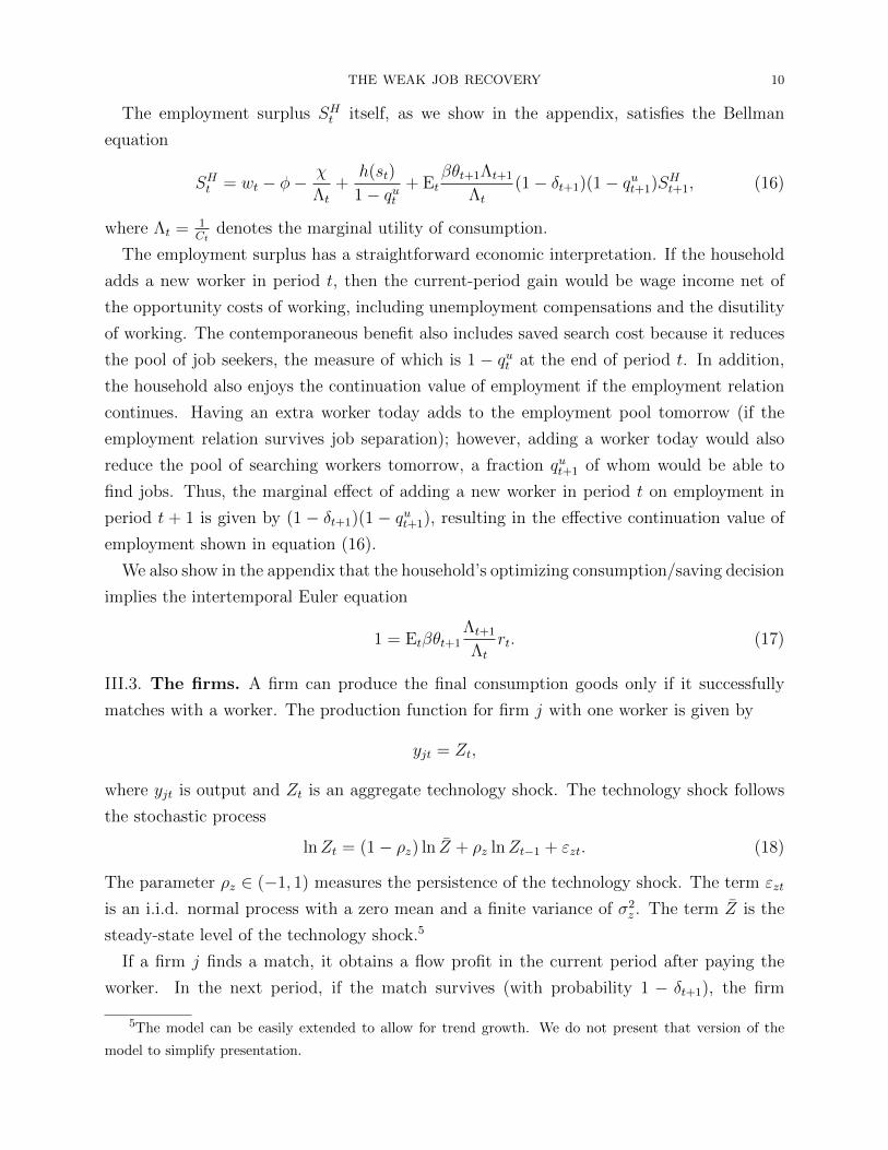
The employment surplus SHt itself, as we show in the appendix, satisfies the Bellman
equation
SHt = wt − φ−χ
Λt
+h(st)
1− qut+ Et
βθt+1Λt+1
Λt
(1− δt+1)(1− qut+1)SHt+1, (16)
where Λt = 1Ct
denotes the marginal utility of consumption.
The employment surplus has a straightforward economic interpretation. If the household
adds a new worker in period t, then the current-period gain would be wage income net of
the opportunity costs of working, including unemployment compensations and the disutility
of working. The contemporaneous benefit also includes saved search cost because it reduces
the pool of job seekers, the measure of which is 1 − qut at the end of period t. In addition,
the household also enjoys the continuation value of employment if the employment relation
continues. Having an extra worker today adds to the employment pool tomorrow (if the
employment relation survives job separation); however, adding a worker today would also
reduce the pool of searching workers tomorrow, a fraction qut+1 of whom would be able to
find jobs. Thus, the marginal effect of adding a new worker in period t on employment in
period t + 1 is given by (1 − δt+1)(1 − qut+1), resulting in the effective continuation value of
employment shown in equation (16).
We also show in the appendix that the household’s optimizing consumption/saving decision
implies the intertemporal Euler equation
1 = Etβθt+1Λt+1
Λt
rt. (17)
III.3. The firms. A firm can produce the final consumption goods only if it successfully
matches with a worker. The production function for firm j with one worker is given by
yjt = Zt,
where yjt is output and Zt is an aggregate technology shock. The technology shock follows
the stochastic process
lnZt = (1− ρz) ln Z + ρz lnZt−1 + εzt. (18)
The parameter ρz ∈ (−1, 1) measures the persistence of the technology shock. The term εzt
is an i.i.d. normal process with a zero mean and a finite variance of σ2z . The term Z is the
steady-state level of the technology shock.5
If a firm j finds a match, it obtains a flow profit in the current period after paying the
worker. In the next period, if the match survives (with probability 1 − δt+1), the firm
5The model can be easily extended to allow for trend growth. We do not present that version of the
model to simplify presentation.
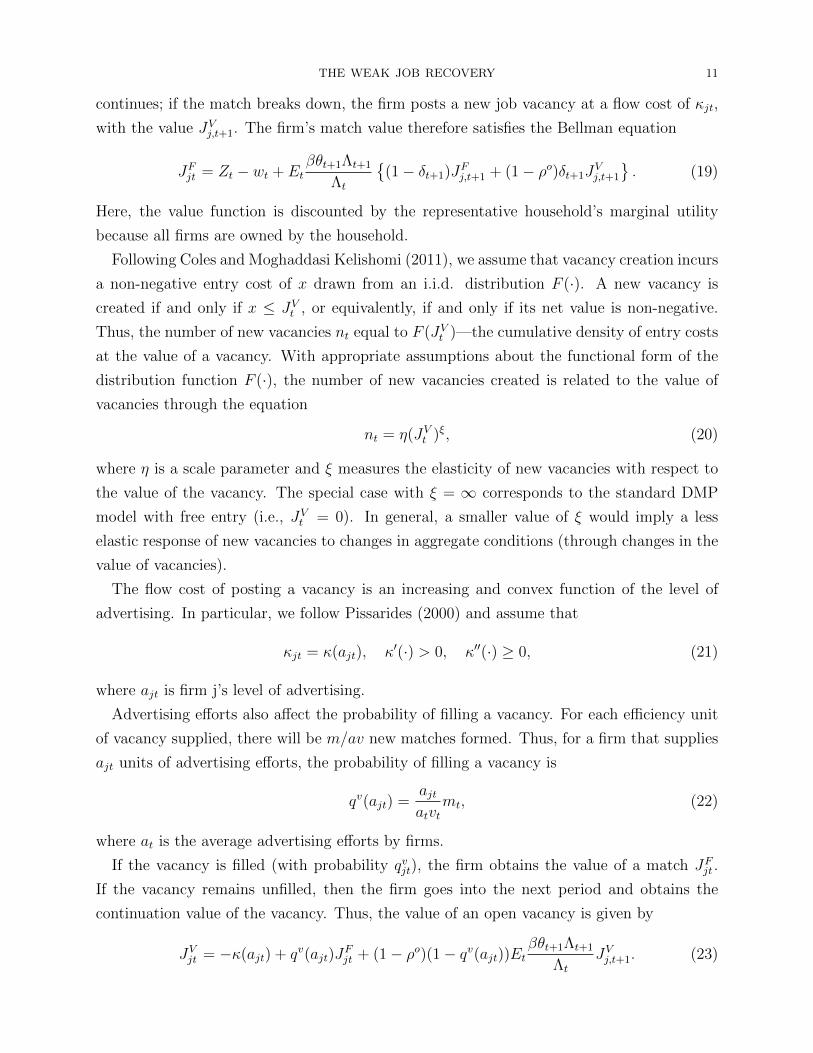
THE WEAK JOB RECOVERY 11
continues; if the match breaks down, the firm posts a new job vacancy at a flow cost of κjt,
with the value JVj,t+1. The firm’s match value therefore satisfies the Bellman equation
JFjt = Zt − wt + Etβθt+1Λt+1
Λt
(1− δt+1)JFj,t+1 + (1− ρo)δt+1J
Vj,t+1
. (19)
Here, the value function is discounted by the representative household’s marginal utility
because all firms are owned by the household.
Following Coles and Moghaddasi Kelishomi (2011), we assume that vacancy creation incurs
a non-negative entry cost of x drawn from an i.i.d. distribution F (·). A new vacancy is
created if and only if x ≤ JVt , or equivalently, if and only if its net value is non-negative.
Thus, the number of new vacancies nt equal to F (JVt )—the cumulative density of entry costs
at the value of a vacancy. With appropriate assumptions about the functional form of the
distribution function F (·), the number of new vacancies created is related to the value of
vacancies through the equation
nt = η(JVt )ξ, (20)
where η is a scale parameter and ξ measures the elasticity of new vacancies with respect to
the value of the vacancy. The special case with ξ = ∞ corresponds to the standard DMP
model with free entry (i.e., JVt = 0). In general, a smaller value of ξ would imply a less
elastic response of new vacancies to changes in aggregate conditions (through changes in the
value of vacancies).
The flow cost of posting a vacancy is an increasing and convex function of the level of
advertising. In particular, we follow Pissarides (2000) and assume that
κjt = κ(ajt), κ′(·) > 0, κ′′(·) ≥ 0, (21)
where ajt is firm j’s level of advertising.
Advertising efforts also affect the probability of filling a vacancy. For each efficiency unit
of vacancy supplied, there will be m/av new matches formed. Thus, for a firm that supplies
ajt units of advertising efforts, the probability of filling a vacancy is
qv(ajt) =ajtatvt
mt, (22)
where at is the average advertising efforts by firms.
If the vacancy is filled (with probability qvjt), the firm obtains the value of a match JFjt .
If the vacancy remains unfilled, then the firm goes into the next period and obtains the
continuation value of the vacancy. Thus, the value of an open vacancy is given by
JVjt = −κ(ajt) + qv(ajt)JFjt + (1− ρo)(1− qv(ajt))Et
βθt+1Λt+1
Λt
JVj,t+1. (23)
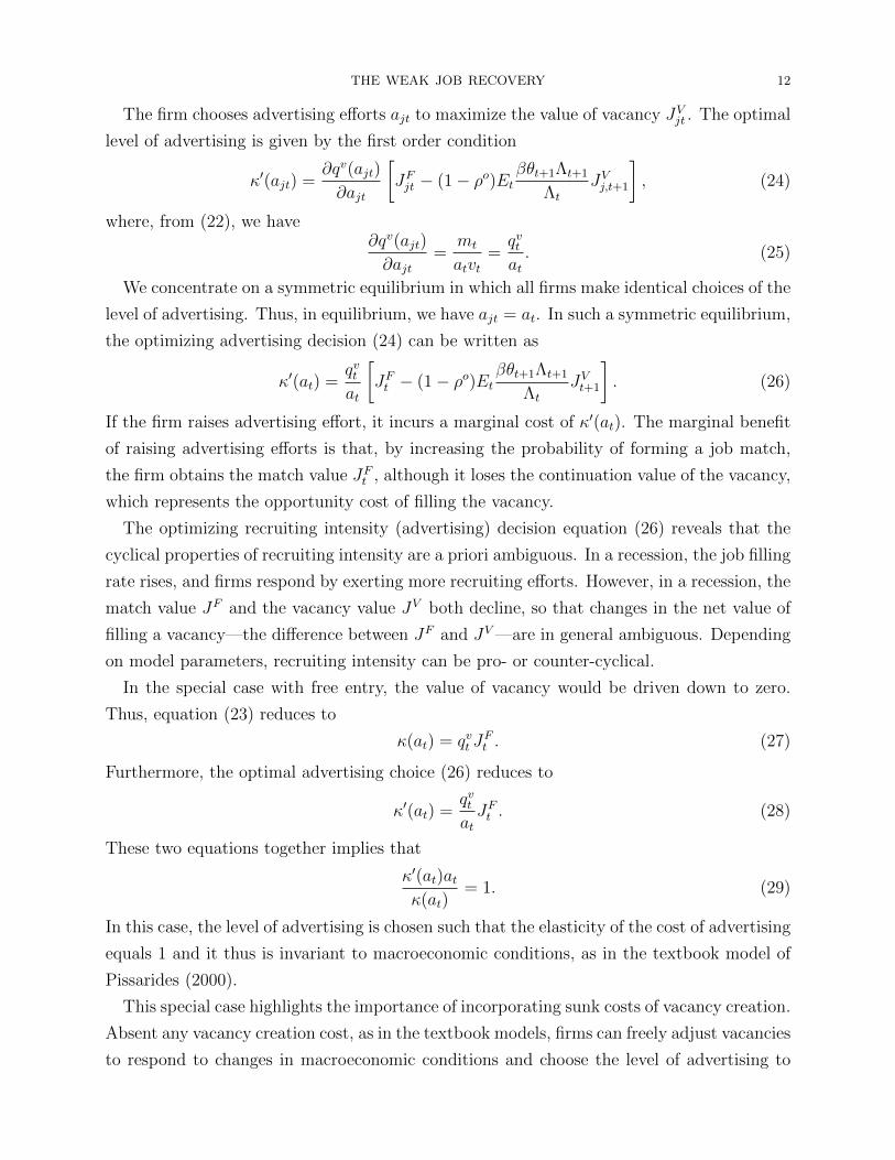
THE WEAK JOB RECOVERY 12
The firm chooses advertising efforts ajt to maximize the value of vacancy JVjt . The optimal
level of advertising is given by the first order condition
κ′(ajt) =∂qv(ajt)
∂ajt
[JFjt − (1− ρo)Et
βθt+1Λt+1
Λt
JVj,t+1
], (24)
where, from (22), we have∂qv(ajt)
∂ajt=
mt
atvt=qvtat. (25)
We concentrate on a symmetric equilibrium in which all firms make identical choices of the
level of advertising. Thus, in equilibrium, we have ajt = at. In such a symmetric equilibrium,
the optimizing advertising decision (24) can be written as
κ′(at) =qvtat
[JFt − (1− ρo)Et
βθt+1Λt+1
Λt
JVt+1
]. (26)
If the firm raises advertising effort, it incurs a marginal cost of κ′(at). The marginal benefit
of raising advertising efforts is that, by increasing the probability of forming a job match,
the firm obtains the match value JFt , although it loses the continuation value of the vacancy,
which represents the opportunity cost of filling the vacancy.
The optimizing recruiting intensity (advertising) decision equation (26) reveals that the
cyclical properties of recruiting intensity are a priori ambiguous. In a recession, the job filling
rate rises, and firms respond by exerting more recruiting efforts. However, in a recession, the
match value JF and the vacancy value JV both decline, so that changes in the net value of
filling a vacancy—the difference between JF and JV —are in general ambiguous. Depending
on model parameters, recruiting intensity can be pro- or counter-cyclical.
In the special case with free entry, the value of vacancy would be driven down to zero.
Thus, equation (23) reduces to
κ(at) = qvt JFt . (27)
Furthermore, the optimal advertising choice (26) reduces to
κ′(at) =qvtatJFt . (28)
These two equations together implies that
κ′(at)atκ(at)
= 1. (29)
In this case, the level of advertising is chosen such that the elasticity of the cost of advertising
equals 1 and it thus is invariant to macroeconomic conditions, as in the textbook model of
Pissarides (2000).
This special case highlights the importance of incorporating sunk costs of vacancy creation.
Absent any vacancy creation cost, as in the textbook models, firms can freely adjust vacancies
to respond to changes in macroeconomic conditions and choose the level of advertising to
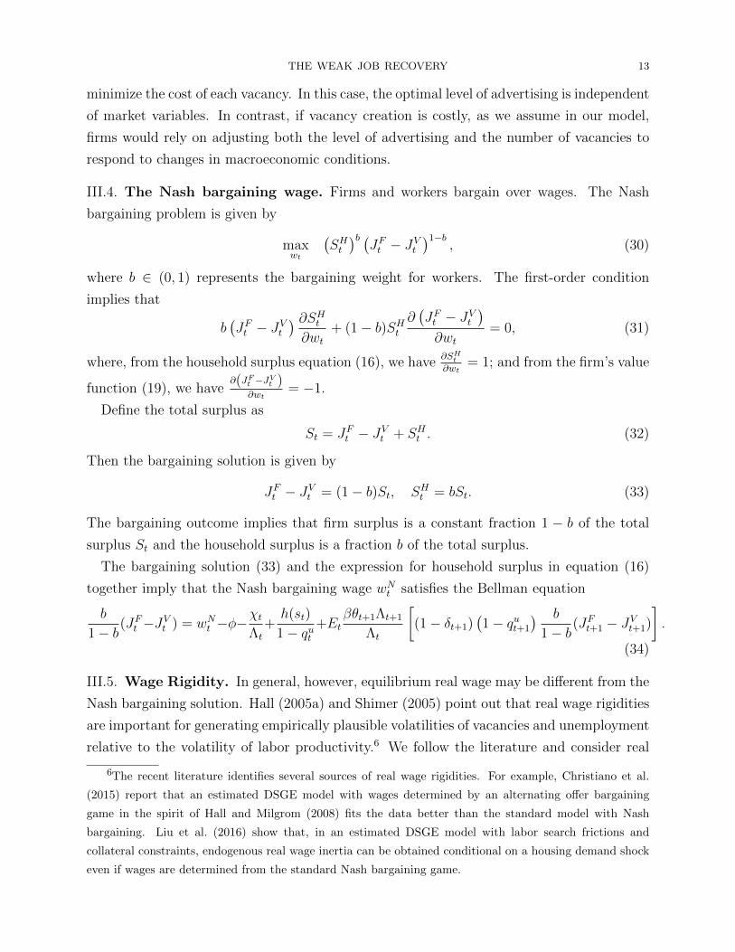
THE WEAK JOB RECOVERY 13
minimize the cost of each vacancy. In this case, the optimal level of advertising is independent
of market variables. In contrast, if vacancy creation is costly, as we assume in our model,
firms would rely on adjusting both the level of advertising and the number of vacancies to
respond to changes in macroeconomic conditions.
III.4. The Nash bargaining wage. Firms and workers bargain over wages. The Nash
bargaining problem is given by
maxwt
(SHt)b (
JFt − JVt)1−b
, (30)
where b ∈ (0, 1) represents the bargaining weight for workers. The first-order condition
implies that
b(JFt − JVt
) ∂SHt∂wt
+ (1− b)SHt∂(JFt − JVt
)∂wt
= 0, (31)
where, from the household surplus equation (16), we have∂SH
t
∂wt= 1; and from the firm’s value
function (19), we have∂(JF
t −JVt )
∂wt= −1.
Define the total surplus as
St = JFt − JVt + SHt . (32)
Then the bargaining solution is given by
JFt − JVt = (1− b)St, SHt = bSt. (33)
The bargaining outcome implies that firm surplus is a constant fraction 1 − b of the total
surplus St and the household surplus is a fraction b of the total surplus.
The bargaining solution (33) and the expression for household surplus in equation (16)
together imply that the Nash bargaining wage wNt satisfies the Bellman equation
b
1− b(JFt −JVt ) = wNt −φ−
χtΛt
+h(st)
1− qut+Et
βθt+1Λt+1
Λt
[(1− δt+1)
(1− qut+1
) b
1− b(JFt+1 − JVt+1)
].
(34)
III.5. Wage Rigidity. In general, however, equilibrium real wage may be different from the
Nash bargaining solution. Hall (2005a) and Shimer (2005) point out that real wage rigidities
are important for generating empirically plausible volatilities of vacancies and unemployment
relative to the volatility of labor productivity.6 We follow the literature and consider real
6The recent literature identifies several sources of real wage rigidities. For example, Christiano et al.
(2015) report that an estimated DSGE model with wages determined by an alternating offer bargaining
game in the spirit of Hall and Milgrom (2008) fits the data better than the standard model with Nash
bargaining. Liu et al. (2016) show that, in an estimated DSGE model with labor search frictions and
collateral constraints, endogenous real wage inertia can be obtained conditional on a housing demand shock
even if wages are determined from the standard Nash bargaining game.

THE WEAK JOB RECOVERY 14
wage rigidity. We assume that the real wage is a geometrically weighted average of the Nash
bargaining wage and the realized wage rate in the previous period. That is,
wt = wγt−1(wNt )1−γ, (35)
where γ ∈ (0, 1) represents the degree of real wage rigidity.7
III.6. Government policy. The government finances unemployment benefit payments φ
for unemployed workers through lump-sum taxes. We assume that the government balances
the budget in each period so that
φ(1−Nt) = Tt. (36)
III.7. Search equilibrium. In a search equilibrium, the markets for bonds and goods all
clear. Since the aggregate supply of bond is zero, the bond market-clearing condition implies
that
Bt = 0. (37)
Aggregate output Yt is related to employment through the aggregate production function
Yt = ZtNt. (38)
Goods market clearing requires that real spendings on consumption, search efforts, re-
cruiting efforts, and vacancy creation equal to aggregate output. This requirement yields
that the aggregate resource constraint
Ct + h(st)ut + κ(at)vt +
∫ JVt
0
xdF (x) = Yt, (39)
where the last term on the left-hand side of the equation corresponds to the aggregate cost of
creating job vacancies. Under our distribution assumption of the vacancy creation cost, the
cumulative density function of x is given by F (x) = ηxξ. Thus, the aggregate cost of vacancy
creation is given by∫ JV
t
0xdF (x) = ηξ
1+ξ(JV )1+ξ. Using the relation between the number of
job vacancies and the value of an open vacancy in equation (20), the aggregate resource cost
for vacancy creation can be written as ξ1+ξ
ntJVt .
7We have examined other wage rules as those in Blanchard and Galı (2010) and we find that our results
do not depend on the particular form of the wage rule.
THE WEAK JOB RECOVERY 15
IV. Empirical strategies
We solve the DSGE model by log-linearzing the equilibrium conditions around the de-
terministic steady state.8 We calibrate a subset of the parameters to match steady-state
observations and estimate the remaining structural parameters and shock processes to fit
the U.S. time series data.
We begin with parameterizing the vacancy cost function κ(a) and search cost function
h(s). We assume that these cost functions are both quadratic and take the forms
κ(at) = κ0 + κ1(at − a) +κ2
2(at − a)2, (40)
h(st) = h1(st − s) +h2
2(st − s)2, (41)
where we normalize the steady-state levels of recruiting intensity and search intensity so that
a = 1 and s = 1.9 We also assume that the search cost is zero in the steady state.
We first calibrate a subset of model parameters using steady-state restrictions. These
parameters include β, the subjective discount factor; χ, the dis-utility of working; α, the
elasticity of matching with respect to searching workers; µ, the matching efficiency; δ, the
average job separation rate; ρo, the vacancy obsolescence rate; φ, the flow unemployment
benefits; b, the Nash bargaining weight; κ0 and κ1, the intercept and the slope of the vacancy
cost function; h1, the slope parameter of the search cost function; γ, the parameter that
measures real wage rigidities; and ξ, the elasticity parameter of vacancy creation.
We estimate the remaining structural and shock parameters using Bayesian methods to
fit the time-series data of unemployment, vacancies, and search intensity. The structural
parameters to be estimated include K ≡ 1η, the scale of the vacancy-creation cost function;
κ2, the curvature of the vacancy-posting cost function; and h2, the curvature of the search
cost function. The shock parameters include ρz and σz, the persistence and the standard
deviation of the technology shock; ρθ and σθ, the persistence and the standard deviation of
the discount factor shock, and ρδ and σδ, the persistence and the standard deviation of the
job separation shock.
IV.1. Calibration. The calibrated values of the model parameters are summarized in Ta-
ble 1.
8Details of the equilibrium conditions, the steady state, and the log-linearized system are available in the
online appendix at http://www.frbsf.org/economic-research/files/wp2016-09_appendix.
pdf.9The quadratic form of the search cost function is supported by the empirical evidence provided by
Yashiv (2000) and Christensen et al. (2005).
THE WEAK JOB RECOVERY 16
We consider a monthly model. Thus, we set β = 0.9967, so that the model implies a
steady-state annualized real interest rate of about 4 percent. We set α = 0.5 following the
literature (Blanchard and Galı, 2010; Gertler and Trigari, 2009). We set the steady-state
job separation rate to δ = 0.034 per month, consistent with the JOLTS data for the period
from December 2000 to April 2015. Following Hall and Milgrom (2008), we set φ = 0.25
so that the unemployment benefit is about 25 percent of normal earnings. We set b = 0.5
following the literature. In our baseline experiment, we follow the literature and set ξ = 1,
as in Fujita and Ramey (2007) and Coles and Moghaddasi Kelishomi (2011).10
We set a value for the steady-state level of vacancy cost κ0 so that the total cost of posting
vacancies is about 1 percent of gross output. To assign a value of κ0 then requires knowledge
of the steady-state number of vacancies v and the steady-state level of output Y .
Given the job separation rate of δ = 0.034 and our calibrated steady-state unemployment
rate of U = 0.055, we obtain the steady-state hiring rate of m = δ(1−U) = 0.0321. We then
calibrate the steady-state value of v such that the model’s steady-state job filling rate qv = mv
matches that in the data. In particular, we match the daily job filling rate of 0.05 estimated
by Davis et al. (2013) using establishment-level JOLTS data. This implies a monthly job
filling rate of qv = 0.6415.11
Given the calibrated values of m and qv, we obtain the steady-state vacancy rate of
v = mqv
= 0.05 To obtain a value for Y , we use the aggregate production function that
Y = ZN and normalize the level of technology such that Z = 1. This procedure yields
a calibrated value of κ0 = 0.1887. We set κ1 = 0.2072 so that the steady-state recruiting
intensity is a = 1. We set h1 = 0.1123 so that the steady-state search intensity is s = 1.
Given the steady-state values of m, u, and v, we use the matching function to obtain
an average matching efficiency of µ = 0.4864. We calibrate the vacancy obsolescence rate
to ρo = 0.0353, so that the steady-state ratio of newly created vacancies to employment in
the model equals 0.036, the same ratio as that estimated by Davis et al. (2013) based on
establishment-level JOLTS data.
To obtain a value for χ, we solve the steady-state system so that χ is consistent with
an unemployment rate of 5.5 percent. The process results in χ = 0.666. Finally, as in the
standard DMP model, our model relies on real wage rigidities to generate the observed large
10When we fix ξ at 0.5 or 2, the quantitative results are similar to our benchmark model. However, if
ξ is fixed at a larger value of 10, the model performs less well, because in that case, the model becomes
closer to one with free entry. For details, see the online appendix available at http://www.frbsf.org/
economic-research/files/wp2016-09_appendix.pdf.11Assuming that one month consists of 20 business days. We can then infer the monthly job filling rate
qv from the daily rate f = 0.05 by using the relation qv = f + f(1 − f) + f(1 − f)2 + · · · + f(1 − f)19 =
1− (1− f)20 = 0.6415.
THE WEAK JOB RECOVERY 17
fluctuations in labor market variables (Shimer, 2005). We set the wage rigidity parameter
to γ = 0.95, which lies at the high end of the literature (Hall, 2005b).
IV.2. Estimation. We now describe our data and estimation approach.
IV.2.1. Data and measurement. We fit the DSGE model to three monthly time-series data
of the U.S. labor market: the unemployment rate, the job vacancy rate, and a measure of
search intensity. The sample covers the period from July 1967 to July 2017.
The unemployment rate in the data (denoted by Udatat ) corresponds to the end-of-period
unemployment rate in the model Ut. We demean the unemployment rate data (in log units)
and relate it to our model variable according to
ln(Udatat )− ln(Udata) = Ut, (42)
where Udata denotes the sample average of the unemployment rate in the data and Ut denotes
the log-deviations of the unemployment rate in the model from its steady-state value.
Similarly, we relate the demeaned vacancy rate data (also in log units) and relate it to the
model variable according to the relation
ln(vdatat )− ln(vdata) = vt, (43)
where vdata denotes the sample average of the vacancy rate data and vt denotes the log-
deviations of the vacancy rate in the model from its steady-state value.
Our measure of search intensity is constructed by Davis (2011). He combines mean un-
employment spells from the Current Population Survey (CPS) and regression results from
Krueger and Mueller (2011), who find that search intensity declines as the duration of un-
employment increases in high-frequency longitudinal data. In particular, Davis (2011) pos-
tulates that
st = A−Bdt, (44)
where st is search intensity and dt is the mean unemployment duration (in weeks). He then
constructs the search intensity index by setting A = 122.30 and B = 0.90 after adjusting
for some potential biases in the regression results obtained by Krueger and Mueller (2011).12
We follow the same methodology as Davis (2011) in constructing a search intensity series,
with the exception that we use the median unemployment duration in weeks instead of the
mean.13
12See the discussions of this methodology in Davis (2011), p.66.13In the Great Recession period, some workers experienced extremely long spells of unemployment, con-
tributing to the sharp increase in the mean duration of unemployment for this period. For this reason, we
use the median unemployment duration to construct our search intensity series, and we believe this median
measure better reflects the underlying factors that influence an individual job seeker’s search efforts than

THE WEAK JOB RECOVERY 18
Figure 3 displays this measure of aggregate search intensity. Clearly, search intensity is
procyclical, rising in booms and falling in recessions. In the Great Recession and its after-
math, search intensity declined substantially, as the duration of unemployment lengthened.
We discuss in Section V.3.2 the importance of using the time series data of search intensity
to discipline the estimation of our DSGE model and to bring the model’s predictions of labor
market variables closer to those in the data.
IV.2.2. Prior distributions and posterior estimates. The prior and posterior distributions of
the estimated parameters from our benchmark model are displayed in Table 2 (Panel A).
The priors of the structural parameters K, κ2, and h2 each follows the gamma distribu-
tion. We assume that the prior mean of K is 5 with a standard deviation of 1. The prior
distribution of κ2 and h2 each has a mean of 1 and a standard deviation of 0.1. For the
shock parameters, we follow the literature and assume that the priors of ρz, ρθ, and ρδ each
follows the beta distribution and the priors of σz, σθ, and σδ each follows an inverse gamma
distribution.
The posterior estimates and the 90% confidence interval for the posterior distributions
are displayed in the last three columns of Table 2. The posterior mean estimate of vacancy
creation cost parameter is K = 5.29, implying a modest steady-state share of vacancy
creation costs of about 0.32 percent of aggregate output. The posterior mean estimates of
curvature parameters of the vacancy posting cost function and of the search cost functions
are κ2 = 1.42 and h2 = 1.47, respectively. The 90% confidence intervals suggest that these
curvature parameters are significantly different from their priors and thus, the data are
informative on these structural parameters.
Our estimation of the shock parameters suggests that technology shocks are less persistent
and less volatile than discount factor shocks and job separation shocks. The AR(1) coefficient
of the technology shock (0.64) is also somewhat smaller than that calibrated in the literature
(e.g., Shimer (2005)). The standard deviation of the innovation to the technology shock
(0.0156) is more in line with the calibration literature.
The discount factor shock is estimated to be persistent, with a monthly AR(1) parameter
of 0.92 and a standard deviation of the innovation of 0.0157. These parameters are broadly
in line with the literature. For example, Hall (2017) estimates a Markov-chain process of the
discount factor shock using the U.S. stock market data. His estimation implies a monthly
persistence parameter of 0.99 and a standard deviation of the innovation of about 0.02.14
does the mean. The time series of median unemployment durations from the BLS is available from July
1967 and on.14These values are calculated based on Figure 5 in Hall (2017) and the descriptions in Section V.A. Under
his estimation, a one standard deviation shock leads to an increase in the discount rate from 8.3 to 10.2 on
THE WEAK JOB RECOVERY 19
The job separation shock is also estimated to be persistent, with a monthly AR(1) co-
efficient of 0.93. It’s standard deviation is larger than the other shocks, at 0.078. These
estimated values are also broadly in line with the standard caliration in the literature. For
example, Shimer (2005) calibrates the quarterly persistence parameter of the job separation
shock to 0.733, corresponding to a monthly value of 0.7331/3 = 0.90. He also calibrates the
standard deviation of the job separation shock to 0.075, which is remarkably similar to our
estimation.
V. Economic implications
We now discuss the economic mechanism through which search and recruiting intensity
help amplify and propagate the impact of the shocks on labor market dynamics in our model.
We also examine the estimated model’s quantitative performance for explaining the sharp
labor-market downturns during the Great Recession and the subsequent weak job recovery.
V.1. The model’s transmission mechanism. To help understand the role of different
shocks in driving labor market dynamics in our model and the model’s propagation mecha-
nism, we examine forecast error variance decompositions and impulse response functions.
V.1.1. Forecast error variance decompositions. Table 3 displays the conditional forecast er-
ror variance decompositions for several key labor market variables and aggregate output.
We focus on the time horizons between 12 months and 48 months, which capture cyclical
fluctuations in these aggregate variables.
Consistent with the intuition provided by Shimer (2005), real wage rigidities in our model
allow technology shocks to play an important role in driving labor market fluctuations. The
variance decomposition results suggest that technology shocks account for 60-80% of the
cyclical fluctuations in unemployment, vacancies, hiring, search intensity, and the job filling
and finding rates, accounting for 60-80% of the variances of these variables. Technology
shocks are also the primarily driving force of recruiting intensity, accounting for about 90%
of its fluctuations.
A discount factor shock can directly affect the present values of a job match, an open
vacancy, and the employment surplus for a job seeker. Thus, it is also potentially important
for explaining the observed labor market fluctuations (Hall, 2017). Quantitatively, our vari-
ance decomposition shows that a discount factor shock contributes to a significant fraction—
impact, which gradually returns to the ergodic mean of 8.3 in about 48 months. The monthly persistence
parameter ρθ = 0.99 is inferred from this information, since θ48 = ρ47θ θ1, where θ48 = 8.3 and θ1 = 10.2. The
initial size of the increase in the discount rate from 8.3 to 10.2 represents a one standard deviation increase
in θt, so we have std(θ) = (10.2 − 8.3)/8.3 = 0.2289. Given the AR(1) coefficient of 0.9956, the standard
deviation of the innovation is given by σθ = std(θ)√
1− ρ2θ = 0.0214.
THE WEAK JOB RECOVERY 20
about 20-30%—of fluctuations in unemployment, vacancies, search intensity, and the job fill-
ing and finding rates. It also contributes to fluctuations in recruiting intensity and hiring,
albeit to a lesser extent (about 10-15%).
A job separations shock also contributes modestly to fluctuations in unemployment, vacan-
cies, and hiring, accounting for about 10-20% of their variances. The shock is unimportant
for the other variables. As noted by Shimer (2005), a job separation shock generates a coun-
terfactually positive correlation between unemployment and vacancies. Accordingly, in our
estimated model, this shock plays a relatively minor role.
V.1.2. Impulse responses. To further understand the model’s transmission mechanism for
each shock, we examine impulse responses. Figure 5 shows the impulse responses of several
key labor market variables to a one standard deviation negative technology shock. The
decline in productivity reduces the value of new job matches. Firms respond by reducing
hiring and vacancy postings. These responses lead to a drop in workers’ job finding rate and
an increase in the unemployment rate.
Unlike the standard model with free entry, our model with costly vacancy creation im-
plies that the value of an unfilled vacancy is non-zero. Thus, as we have alluded to in the
introduction, vacancies become a state variable that evolves slowly over time according to
the law of motion in Equation (3). This gives rise to persistent dynamics in vacancies, as
shown in Figure 5. The initial drop in the stock of vacancies is attributable to declines in
newly created vacancies: since the shock reduces the value of an open vacancy (JVt ), firms
have less incentive to create new vacancies.
The figure also shows that a contractionary technology shock reduces both search intensity
and recruiting intensity. The household’s optimizing decisions for search intensity (Eq. (15))
show that search intensity increases with the job finding probability and the employment
value, which is proportional to the match surplus from Nash bargaining. Since the technology
shock lowers both the job finding rate and the match surplus, it reduces search intensity as
well.
Recruiting intensity falls following the negative technology shock partly because the ex-
pected value of a job match declines. This can be seen from the optimizing decision for
recruiting intensity in Equation (26), which shows that recruiting intensity increases with
both the job filling probability and the value of a new job match (JF ) relative to the value of
an unfilled vacancy (JV ). However, because the technology shock reduces both JF and JV ,
the net effect on recruiting intensity can be ambiguous. Under our estimated parameters,
the net surplus falls following a contractionary technology shock. Thus, recruiting intensity
falls as well.
THE WEAK JOB RECOVERY 21
Declines in search and recruiting intensity counteract the effects of the rise in unemploy-
ment on hiring and reinforce the effects of the drop in vacancies. The net effect leads to a
fall in hiring. With both hiring and vacancies declining following the negative technology
shock, the response of the job filling rate—which is the ratio of hires to vacancies— can
be ambiguous. Under our estimation, the job filling rate rises initially and then falls below
steady state before returning to it.
As search intensity and recruiting intensity both decline, the technology shock leads to
a decline in the measured matching efficiency and thus an outward shift of the Beveridge
curve. The measured matching efficiency here is defined as
Ωt = µsαt a1−αt . (45)
Although there are no exogenous changes in true matching efficiency (i.e., if µ is constant),
measured matching efficiency (Ω) in our model still fluctuates with endogenous variations in
search and recruiting intensity.
The variance decompositions in Table 3 suggest that, in addition to technology shocks,
shocks to the discount factor and the job separation rate in our model also contribute to
the observed labor market fluctuations. We now turn to discussing the impulse responses
following those shocks.
Figures 6 shows the impulse responses of labor market variables following a one standard
deviation negative discount factor shock. The shock lowers the continuation value of a job
match, leading to declines in hiring. Since the shock lowers the employment surplus, search
intensity declines. Recruiting intensity also falls because the decline in the present value of
a new job match outweighs that in the value of an open vacancy. Firms respond to the drop
in vacancy value by creating and posting fewer vacancies. The job filling rate increases, as
the decline in vacancies outweighs the fall in hiring.
Figures 7 shows the impulse responses following a positive shock to the job separation
rate. With a higher rate of job separation, the unemployment rate rises. At the same time,
separated jobs add to the stock of vacancies, so that the vacancy rate rises as well. Since
both u and v increase, the hiring rate also rises. Equilibrium adjustments of hiring also
depend on the responses of the intensive margins. The job separation shock reduces both
the match value JF and the vacancy value JV , rendering the net effect on recruiting intensity
ambiguous. Under our estimation, recruiting intensity edges down following the separation
shock. On the other hand, since firms reduce the number of newly created vacancies in
response to the shock, households choose to reduce search intensity slightly. On net, the job
separation shock leads to only small responses of these intensive margins. It follows that the
job filling and finding rates are both driven mostly by the labor market tightness (the v− u

THE WEAK JOB RECOVERY 22
ratio). Since the shock leads to an increase in both v and u, its impact on the job filling and
finding rates are small.
V.2. The Great Recession and the weak job recovery. The impulse responses show
that search and recruiting intensity are both procyclical in our estimated model. We now
show that procyclical fluctuations in these intensive margins significantly improve the model’s
ability to quantitatively capture the observed labor market dynamics during the Great Re-
cession and the subsequent recovery.
Figure 1 shows that, in the data (the blue solid lines), the job filling rate rose sharply and
the job finding rate declined sharply during the Great Recession, and they both recovered
gradually to pre-recession levels. These patterns are consistent with a sharp downturn in
hiring in the recession and a relatively subdued recovery thereafter.
The standard model without search and recruiting intensity has difficulties in replicating
these observations. As Figure 1 shows (the red dashed lines), the predicted job filling rate
and the job finding rate from the standard matching function diverged from the data since
early 2009, and they both stayed persistently above the data after the recession. Thus,
according to the standard matching function, hiring should not have declined as sharply as
that actually occurred in the recession, and the recovery should have been stronger than
observed.
In comparison, our model with endogenous search intensity and recruiting intensity does
not share these counterfactual predictions from the standard model. As shown in Figure 2
(the black dashed and dotted lines), the predicted job filling and finding rates from our
benchmark model track the actual data closely throughout the recession and recovery peri-
ods.
To get a quantitative sense of the goodness of fit of our model relative to the standard
matching function, we consider the root mean squared errors (RMSE) for the variables of
interest in each model. We calculate the RMSEs based on demeaned series in the data and in
each model from the sample period starting from 2001.15 As shown in Table 4, the standard
matching function’s predicted job filling rate has an RMSE of 0.1086 relative to the data. In
contrast, the RMSE of the job filling rate predicted from our estimated benchmark model is
0.0466, less than half of that implied by the standard matching function. Our model with
search and recruiting intensity also improves the fit for the job finding rate relative to the
standard matching function, with a similar magnitude of improvement.
15The series shown in Figure 2 are normalized based on the demeaned series, so that the first observation
of each series is indexed to 0. We do not calculate the RMSEs based on the normalized series, but instead,
we use the “raw” demeaned series.
THE WEAK JOB RECOVERY 23
It is important to also note that the improved model performance is not trivially attribut-
able to the introduction of search intensity in the matching function. For instance, Table 4
reports the RMSEs of the standard matching function modified to also include our measure
of search intensity.16 The table shows that augmenting the standard matching function with
the observed search intensity by itself does not improve the fit to the data significantly; the
RMSEs from this augmented matching function are marginally smaller than those implied
by the standard matching function (0.0914 vs. 0.1086), both substantially exceeding those
predicted from our DSGE model (0.0466).
Thus, search intensity in our model entails important interactions with recruiting intensity
that help better account for the movements in the job filling and job finding rates since 2007.
One concern is that the improvements in fit during the Great Recession and its aftermath
may come at the cost of a worsening perfomance in periods prior to the Great Recession.
Figure 4 shows that this is not the case. While we focus on the post-2001 period in Figure 2
because of the availability of JOLTS data, we still estimate our model over a longer period
(starting from July 1967) that captures several business cycles. This allows a comparison
of the fluctuations in the job filling and job finding rates from our benchmark model and
from the standard matching function for the periods prior to 2001. In contrast to the Great
Recession and its aftermath, Figure 4 shows that the two models’ predictions track each
other remarkably well before the Great Recession.
The improved ability of our benchmark model to track the observed paths of the job filling
and finding rates since the Great Recession suggests that the model may also be able to
account for the observed weak recovery in hiring. This is only partly true, however. Figure 9
shows the paths of hiring predicted from our benchmark model and that in the actual data,
with the sample starting in December 2000, which is the beginning of the JOLTS sample.
The figure shows that, while the magnitude of declines in hiring predicted from our model
during the Great Recession is roughly in line with that in the data, our model misses the
timing of the trough by about one year. Nonetheless, the correlation between the model’s
predicted hiring rate and the actual hiring rate is still positive and large, at about 0.55,
which is remarkable given that our model is not fitted to the observed time-series data of
hiring.
Our model also implies that recruiting intensity is positively correlated with the hiring
rate, as found by Davis et al. (2013), despite clear differences in the approaches. Davis et al.
(2013) construct a measure of recruiting intensity based on establishment-level data. They
show that recruiting intensity delivers a better-fitting Beveridge curve and accounts for a
16Under the matching function augmented with search intensity, the job filling rate is given by µ(utstvt
)αand the job finding rate is µsαt
(vtut
)1−α, where the variables and the parameters are defined earlier.
THE WEAK JOB RECOVERY 24
large share of fluctuations in aggregate hires. They further impute an aggregate relation
between recruiting intensity and the hiring rate based on their estimated microeconomic
relations. They show that this aggregate measure of recruiting intensity is highly correlated
with the aggregate hiring rate, with a sample correlation of about 0.82.
We have followed a very different approach to obtaining an empirical measure of recruiting
intensity (at) in our estimated macro model. To assess the cyclical behaviors of our measure
of recruiting intensity, we calculated the sample correlation between the model-based time
series of recruiting intensity and the hiring rate. We obtained a correlation of 0.48, which is
lower than that reported by Davis et al. (2013), though still significantly positive. We view
our result as strengthening the argument by Davis et al. (2013) that recruiting intensity is
procyclical and it plays an important role in explaining cyclical fluctuations in aggregate
hires.
V.3. The importance of search and recruiting intensity. To understand the impor-
tance of cyclical variations in search and recruiting intensity, we conduct two sets of coun-
terfactual experiments. In the first experiment, we consider a counterfactual model with
both search intensity and recruiting intensity held constant. In the second experiment, we
re-estimate the benchmark model to fit time-series data on unemployment and vacancies
only, without using data on search intensity.
V.3.1. A counterfactual model with constant search and recruiting intensity. We first con-
sider a counterfactual model with no cyclical fluctuations in search and recruiting intensity.
In particular, we keep the parameters and the shock processes the same as in the estimated
benchmark model, but we force the search intensity and recruiting intensity to stay constant
at their steady-state levels. We calculate the impulse responses in this counterfactual model
and compare them to those obtained in our benchmark model. We focus on the effects of a
negative technology shock, partly because our variance decompositions show that technology
shocks are the most important shock that drive the labor market dynamics in our model. 17
Figure 8 shows the impulse responses to a negative technology shock in the counterfactual
model with constant search and recruiting intensity (the blue dashed lines), along with those
in the benchmark model (the black solid lines).
The figure highlights that a negative technology shock leads to a more muted decline
in hiring and a smaller increase in unemployment in the counterfactual model than those
predicted by the benchmark model with endogenous intensive-margin adjustments. Without
variations in search and recruiting intensity, hiring is solely determined by the number of
17The qualitatively results under a discount factor shock or a job separation shock are similar. See the
online appendix for details.
THE WEAK JOB RECOVERY 25
job-seekers and the number of job vacancies according to the matching function. Since the
number of job seekers entering the matching function is predetermined and the stock of job
vacancies is a slow-moving state variable, the responses of hiring in the counterfactual model
are more muted than in the benchmark model. With a smaller response of hiring, declines in
vacancies imply a stronger increase in the job filling rate following the negative technology
shock. The counterfactual model also generates smaller declines in the job finding rate than
does the benchmark model.
Overall, Figure 8 shows that endogenous adjustments in search and recruiting intensity
to changes in macroeconomic conditions help amplify the responses of the labor market
variables.
V.3.2. The importance of using information from search intensity data. In estimating our
benchmark model, we have used three time series data: the unemployment rate, the job
vacancy rate, and a measure of search intensity. We followed Davis (2011) and constructed
a time series of search intensity based on the median unemployment duration. The resulting
search intensity series is procyclical, as shown in Figure 3. The procyclical behavior of search
intensity is consistent with the textbook model (Pissarides, 2000).18
Yet, the empirical literature is not conclusive about whether search intensity is procyclical.
For example, in an influential study, Shimer (2004) argues that search intensity is counter-
cyclical based on cross-sectional data of the average number of search methods used by job
seekers observed in the Current Population Survey (CPS). Mukoyama et al. (2014) combine
information from the CPS data and the American Time Use Survey (ATUS) and obtain
similar results.
On the other side of the debate, Tumen (2014) criticizes the interpretation of the cyclical
behavior of search intensity measured by cross-sectional average number of search methods
in the CPS. He emphasizes that these cross-sectional measures are likely to suffer from a
composition bias if a job seeker with stronger labor-market attachment also uses more search
methods, since the share of job seekers with stronger labor-market attachment increases
during a recession. When this composition bias is corrected, Tumen (2014) finds that search
intensity is procyclical. Gomme and Lkhagvasuren (2015) make a similar argument about
the composition bias. They use merged data from the ATUS and the CPS to study cyclical
18The measure of search intensity that we use, which is the same measure used by Davis (2011), has
an advantage in that it is constructed based on estimated parameters using longitudinal data that track
unemployed workers’ amount of time spent for job searching as well as the number of weeks they have been
unemployed. A drawback of this method is that it is based on answers from interviews conducted over a
24-week period during the fall of 2009 and winter of 2010, so the estimation uses a relatively short time-series
dimension.
THE WEAK JOB RECOVERY 26
variations in search intensity. They find that, when the composition bias is corrected, the
evidence suggests procyclical search intensity.19
Given this debate, we assess the robustness of our findings by fitting our model to the
observed unemployment rate and the vacancy rate only. Under this alternative estimation,
we do not use information of search intensity in the data. In this alternative estimation, we
keep the priors of the parameters the same as in our benchmark estimation.
The posterior estimation results are shown in Table 2 (Panel B). Compared to the bench-
mark estimation, this alternative estimation without using information from search intensity
data results in a few notable changes in the posterior distributions of the structural parame-
ters and the shock parameters. In particular, the technology and discount factor shocks are
now much less persistent. Specifically, the posterior mean of the autoregressive coefficients
of the technology shock, ρz, and of the discount factor shock, ρθ, are now significantly lower
at 0.24 and 0.17, respectively, compared to 0.64 and 0.92 in the bechmark estimation. In
addition, the standard deviations of both shocks also decline.
Omitting information from search intensity leads to significantly poorer fit of our model to
the data, as shown in Figure 10. The job filling and finding rates predicted from our model
estimated without using search intensity data still track the data more closely than those from
the standard matching function, but the improvements in fitting are substantially smaller
than those obtained from our benchmark estimation, in which we use search intensity datas.
Table 4 shows that the RMSEs for the job filling rate and the job finding rate predicted from
our model under this alternative estimation are only marginally lower than those implied by
the standard matching function, and significantly worse than our benchmark estimation.
In addition, when we estimate the model without fitting to the search intensity series, the
hiring rate implied by the model displays a much weaker correlation with that in the data
than that obtained from our benchmark estimation. Specifically, the correlation between
model-implied hiring and actual hiring turns negative (-0.17), whereas the benchmark model
displays a sizable positive correlation (0.55). These results suggest that fluctuations in search
intensity are important to account for fluctuations in hiring.
Furthermore, cyclical fluctuations in search intensity also help amplify cyclical fluctuations
in recruiting intensity. When we do not use information from search intensity to estimate
the model, the correlation between recruiting intensity and hiring becomes negative (-0.17),
19Mueller (2017) shows that the pool of unemployed shifts to high-wage workers in recessions. If high-
wage workers search more intensely, this can lead to a substantial composition bias. Faberman and Kudlyak
(2016) also discuss the implications of composition bias in measuring search intensity. They report that
long-term unemployed job seekers tend to exert more efforts throughout their search process, reflecting that
long-term unemployed individuals have stronger labor-market attachment.
THE WEAK JOB RECOVERY 27
compared to the positive correlation in the benchmark model (0.48) and in Davis et al.
(2013).
Overall, these exercises suggest that using our measure of search intensity in estimating the
DSGE model helps discipline the estimation. It also suggests that there are important general
equilibrium interactions between search intensity and recruiting intensity that amplify the
impact of the shocks on labor market variables. Furthermore, procyclical fluctuations in
search intensity and recruiting intensity help bridge the gap between the model’s predicted
job filling and job finding rates and those in the data.
VI. Conclusion
The sharp downturn in hiring during the Great Recession and the weak recovery presented
a challenge for the standard model of labor search and matching. We have developed and
estimated a DSGE model that generalizes the standard model to incorporate cyclical fluctua-
tions of search and recruiting intensity. We find that these intensive margins of labor-market
adjustments are quantitatively important. In the depth of the recession and during the recov-
ery period, the job filling rate and the job finding rate predicted from our estimated model
are much closer to the actual time-series data than those implied by the standard model
without search and recruiting intensity. Our model suggests that the observed deep labor
market recession and the weak recovery stem to a large extent from procyclical fluctuations
in search and recruiting intensity.
To allow for aggregate fluctuations in recruiting intensity, we modify the standard model
by assuming that firms need to pay a fixed cost to create a new job vacancy. This simple
modification facilitates tractability and makes it straightforward to estimate the model to fit
time-series data using standard techniques. Interestingly, our macro emphasis nonetheless
yields predictions of the cyclical movements in recruiting intensity that are very much in line
with those postulated in Davis et al. (2013) based on establishment-level data. In particu-
lar, both approaches highlight a procyclical recruiting intensity. In addition, our empirical
findings also point to an important interaction between search and recruiting intensity that
helps account for the observed behavior of the job filling and job finding rates since the end
of the Great Recession.
To better highlight our model’s mechanism, we focus on three particular sources of busi-
ness cycle fluctuations: technology shocks, discount factor shocks, and job separation shocks.
All these shocks are arguably reduced-form representations of some microeconomic frictions
or policy distortions that are not considered in our model. For example, the discount factor
shock in our model that represents stochastic changes in households’ intertemporal prefer-
ences may reflect factors outside of the model that drive asset market fluctuations (Hall,
THE WEAK JOB RECOVERY 28
2017). Our model also assumes that job separations vary exogenously, while in reality, job
separations occur endogenously in response to the state of the economy.
Our model also restricts the labor force participation rate to be constant. Relaxing this
assumption can have important implications for labor market dynamics. For example, Di-
amond (2013) argues that incorporating flows into and out of the labor force helps bet-
ter understand the shifts of the Beveridge curve after the Great Recession. Kudlyak and
Schwartzman (2012) show that persistent declines in labor force participation contributed to
the large increases in unemployment during the Great Recession and also to the subsequent
slow decline in unemployment. Future research should extend our framework to incorporate
endogenous job separations and labor force participation to study their potential interac-
tions with search and recruiting intensity. Such a framework should be useful for better
understanding labor market fluctuations and for policy designs. Our work provides a step
forward for this promising research agenda.
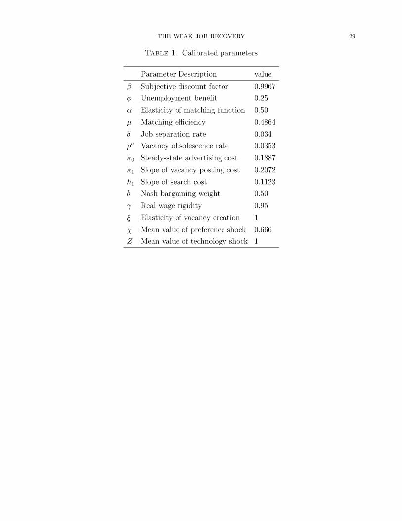
THE WEAK JOB RECOVERY 29
Table 1. Calibrated parameters
Parameter Description value
β Subjective discount factor 0.9967
φ Unemployment benefit 0.25
α Elasticity of matching function 0.50
µ Matching efficiency 0.4864
δ Job separation rate 0.034
ρo Vacancy obsolescence rate 0.0353
κ0 Steady-state advertising cost 0.1887
κ1 Slope of vacancy posting cost 0.2072
h1 Slope of search cost 0.1123
b Nash bargaining weight 0.50
γ Real wage rigidity 0.95
ξ Elasticity of vacancy creation 1
χ Mean value of preference shock 0.666
Z Mean value of technology shock 1
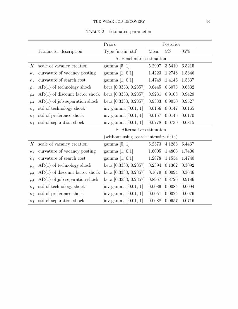
THE WEAK JOB RECOVERY 30
Table 2. Estimated parameters
Priors Posterior
Parameter description Type [mean, std] Mean 5% 95%
A. Benchmark estimation
K scale of vacancy creation gamma [5, 1] 5.2907 3.5410 6.5215
κ2 curvature of vacancy posting gamma [1, 0.1] 1.4223 1.2748 1.5346
h2 curvature of search cost gamma [1, 0.1] 1.4749 1.4146 1.5337
ρz AR(1) of technology shock beta [0.3333, 0.2357] 0.6445 0.6073 0.6832
ρθ AR(1) of discount factor shock beta [0.3333, 0.2357] 0.9231 0.9108 0.9429
ρδ AR(1) of job separation shock beta [0.3333, 0.2357] 0.9333 0.9050 0.9527
σz std of technology shock inv gamma [0.01, 1] 0.0156 0.0147 0.0165
σθ std of preference shock inv gamma [0.01, 1] 0.0157 0.0145 0.0170
σδ std of separation shock inv gamma [0.01, 1] 0.0778 0.0739 0.0815
B. Alternative estimation
(without using search intensity data)
K scale of vacancy creation gamma [5, 1] 5.2373 4.1283 6.4467
κ2 curvature of vacancy posting gamma [1, 0.1] 1.6005 1.4803 1.7406
h2 curvature of search cost gamma [1, 0.1] 1.2878 1.1554 1.4740
ρz AR(1) of technology shock beta [0.3333, 0.2357] 0.2394 0.1362 0.3092
ρθ AR(1) of discount factor shock beta [0.3333, 0.2357] 0.1679 0.0094 0.3646
ρδ AR(1) of job separation shock beta [0.3333, 0.2357] 0.8957 0.8726 0.9186
σz std of technology shock inv gamma [0.01, 1] 0.0089 0.0084 0.0094
σθ std of preference shock inv gamma [0.01, 1] 0.0051 0.0024 0.0076
σδ std of separation shock inv gamma [0.01, 1] 0.0688 0.0657 0.0716
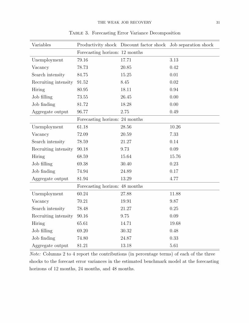
THE WEAK JOB RECOVERY 31
Table 3. Forecasting Error Variance Decomposition
Variables Productivity shock Discount factor shock Job separation shock
Forecasting horizon: 12 months
Unemployment 79.16 17.71 3.13
Vacancy 78.73 20.85 0.42
Search intensity 84.75 15.25 0.01
Recruiting intensity 91.52 8.45 0.02
Hiring 80.95 18.11 0.94
Job filling 73.55 26.45 0.00
Job finding 81.72 18.28 0.00
Aggregate output 96.77 2.75 0.49
Forecasting horizon: 24 months
Unemployment 61.18 28.56 10.26
Vacancy 72.09 20.59 7.33
Search intensity 78.59 21.27 0.14
Recruiting intensity 90.18 9.73 0.09
Hiring 68.59 15.64 15.76
Job filling 69.38 30.40 0.23
Job finding 74.94 24.89 0.17
Aggregate output 81.94 13.29 4.77
Forecasting horizon: 48 months
Unemployment 60.24 27.88 11.88
Vacancy 70.21 19.91 9.87
Search intensity 78.48 21.27 0.25
Recruiting intensity 90.16 9.75 0.09
Hiring 65.61 14.71 19.68
Job filling 69.20 30.32 0.48
Job finding 74.80 24.87 0.33
Aggregate output 81.21 13.18 5.61
Note: Columns 2 to 4 report the contributions (in percentage terms) of each of the three
shocks to the forecast error variances in the estimated benchmark model at the forecasting
horizons of 12 months, 24 months, and 48 months.
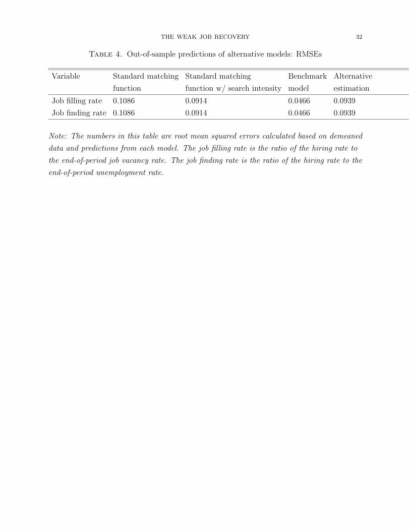
THE WEAK JOB RECOVERY 32
Table 4. Out-of-sample predictions of alternative models: RMSEs
Variable Standard matching Standard matching Benchmark Alternative
function function w/ search intensity model estimation
Job filling rate 0.1086 0.0914 0.0466 0.0939
Job finding rate 0.1086 0.0914 0.0466 0.0939
Note: The numbers in this table are root mean squared errors calculated based on demeaned
data and predictions from each model. The job filling rate is the ratio of the hiring rate to
the end-of-period job vacancy rate. The job finding rate is the ratio of the hiring rate to the
end-of-period unemployment rate.
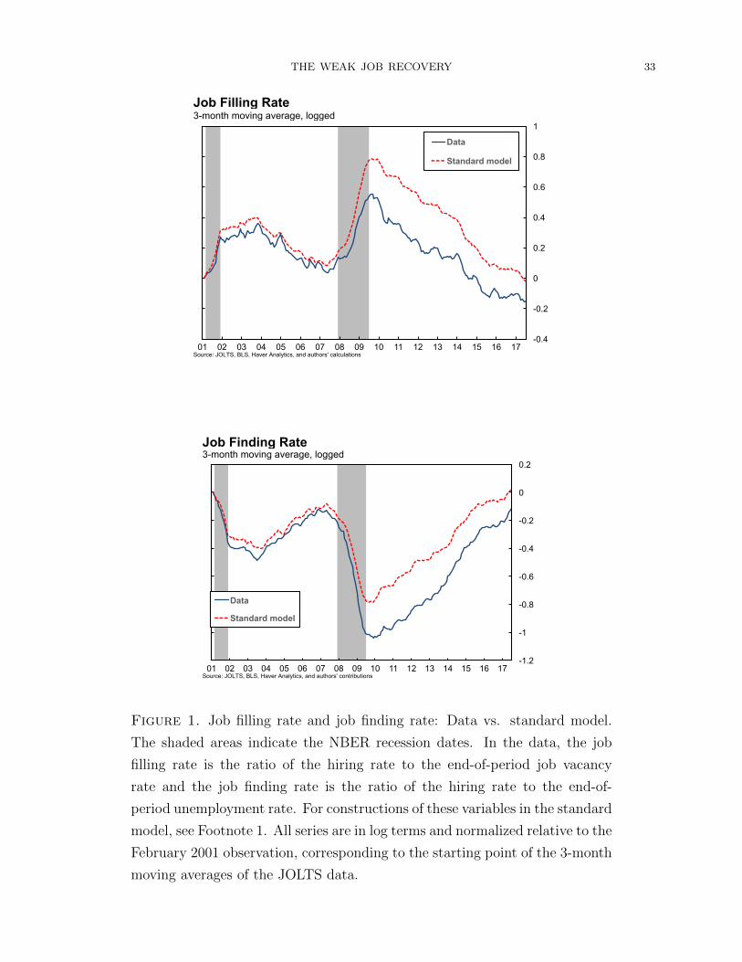
THE WEAK JOB RECOVERY 33
-0.4
-0.2
0
0.2
0.4
0.6
0.8
1
01 02 03 04 05 06 07 08 09 10 11 12 13 14 15 16 17
Data
Standard model
Source: JOLTS, BLS, Haver Analytics, and authors' calculations
3-month moving average, loggedJob Filling Rate
-1.2
-1
-0.8
-0.6
-0.4
-0.2
0
0.2
01 02 03 04 05 06 07 08 09 10 11 12 13 14 15 16 17
Data
Standard model
Source: JOLTS, BLS, Haver Analytics, and authors' contributions
3-month moving average, loggedJob Finding Rate
Figure 1. Job filling rate and job finding rate: Data vs. standard model.
The shaded areas indicate the NBER recession dates. In the data, the job
filling rate is the ratio of the hiring rate to the end-of-period job vacancy
rate and the job finding rate is the ratio of the hiring rate to the end-of-
period unemployment rate. For constructions of these variables in the standard
model, see Footnote 1. All series are in log terms and normalized relative to the
February 2001 observation, corresponding to the starting point of the 3-month
moving averages of the JOLTS data.
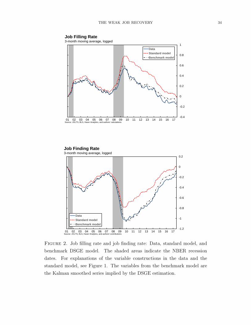
THE WEAK JOB RECOVERY 34
-0.4
-0.2
0
0.2
0.4
0.6
0.8
1
01 02 03 04 05 06 07 08 09 10 11 12 13 14 15 16 17
Data
Standard model
Benchmark model
Source: JOLTS, BLS, Haver Analytics, and authors' calculations
3-month moving average, logged
Job Filling Rate
-1.2
-1
-0.8
-0.6
-0.4
-0.2
0
0.2
01 02 03 04 05 06 07 08 09 10 11 12 13 14 15 16 17
Data
Standard model
Benchmark model
Source: JOLTS, BLS, Haver Analytics, and authors' contributions
3-month moving average, logged
Job Finding Rate
Figure 2. Job filling rate and job finding rate: Data, standard model, and
benchmark DSGE model. The shaded areas indicate the NBER recession
dates. For explanations of the variable constructions in the data and the
standard model, see Figure 1. The variables from the benchmark model are
the Kalman smoothed series implied by the DSGE estimation.
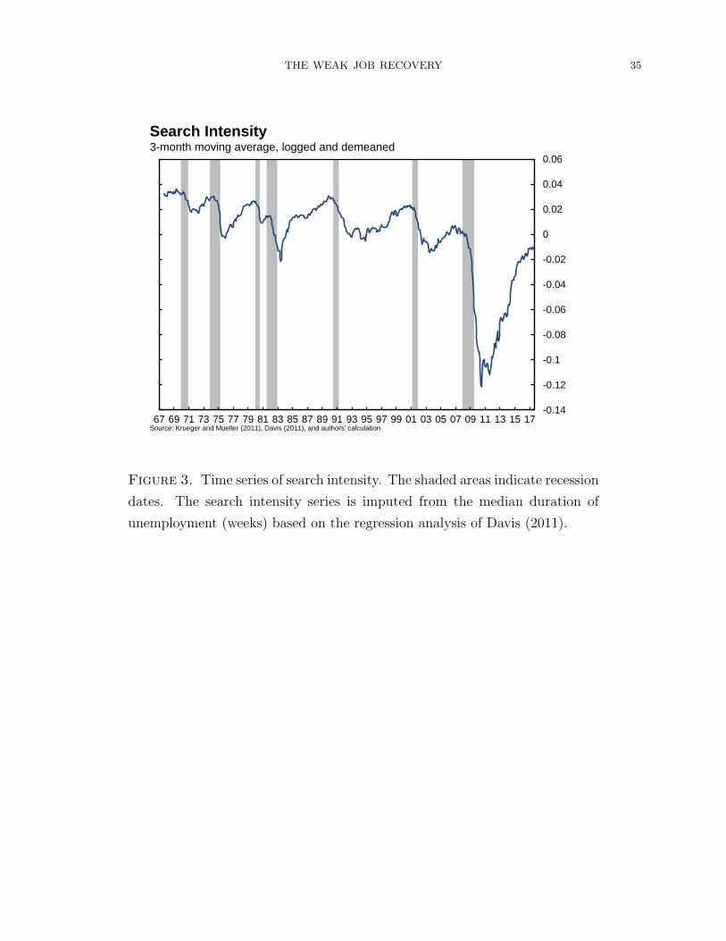
THE WEAK JOB RECOVERY 35
-0.14
-0.12
-0.1
-0.08
-0.06
-0.04
-0.02
0
0.02
0.04
0.06
67 69 71 73 75 77 79 81 83 85 87 89 91 93 95 97 99 01 03 05 07 09 11 13 15 17Source: Krueger and Mueller (2011), Davis (2011), and authors' calculation
3-month moving average, logged and demeaned
Search Intensity
Figure 3. Time series of search intensity. The shaded areas indicate recession
dates. The search intensity series is imputed from the median duration of
unemployment (weeks) based on the regression analysis of Davis (2011).
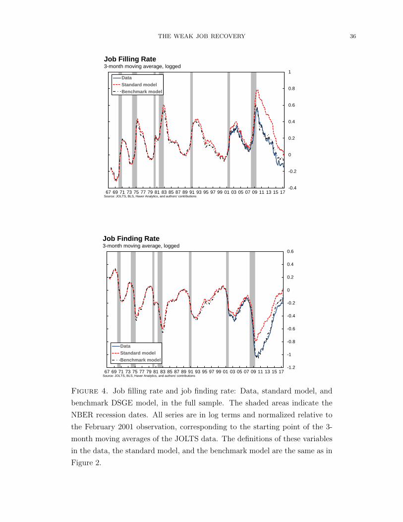
THE WEAK JOB RECOVERY 36
-0.4
-0.2
0
0.2
0.4
0.6
0.8
1
67 69 71 73 75 77 79 81 83 85 87 89 91 93 95 97 99 01 03 05 07 09 11 13 15 17
Data
Standard model
Benchmark model
Source: JOLTS, BLS, Haver Analytics, and authors' contributions
3-month moving average, logged
Job Filling Rate
-1.2
-1
-0.8
-0.6
-0.4
-0.2
0
0.2
0.4
0.6
67 69 71 73 75 77 79 81 83 85 87 89 91 93 95 97 99 01 03 05 07 09 11 13 15 17
Data
Standard model
Benchmark model
Source: JOLTS, BLS, Haver Analytics, and authors' contributions
3-month moving average, logged
Job Finding Rate
Figure 4. Job filling rate and job finding rate: Data, standard model, and
benchmark DSGE model, in the full sample. The shaded areas indicate the
NBER recession dates. All series are in log terms and normalized relative to
the February 2001 observation, corresponding to the starting point of the 3-
month moving averages of the JOLTS data. The definitions of these variables
in the data, the standard model, and the benchmark model are the same as in
Figure 2.
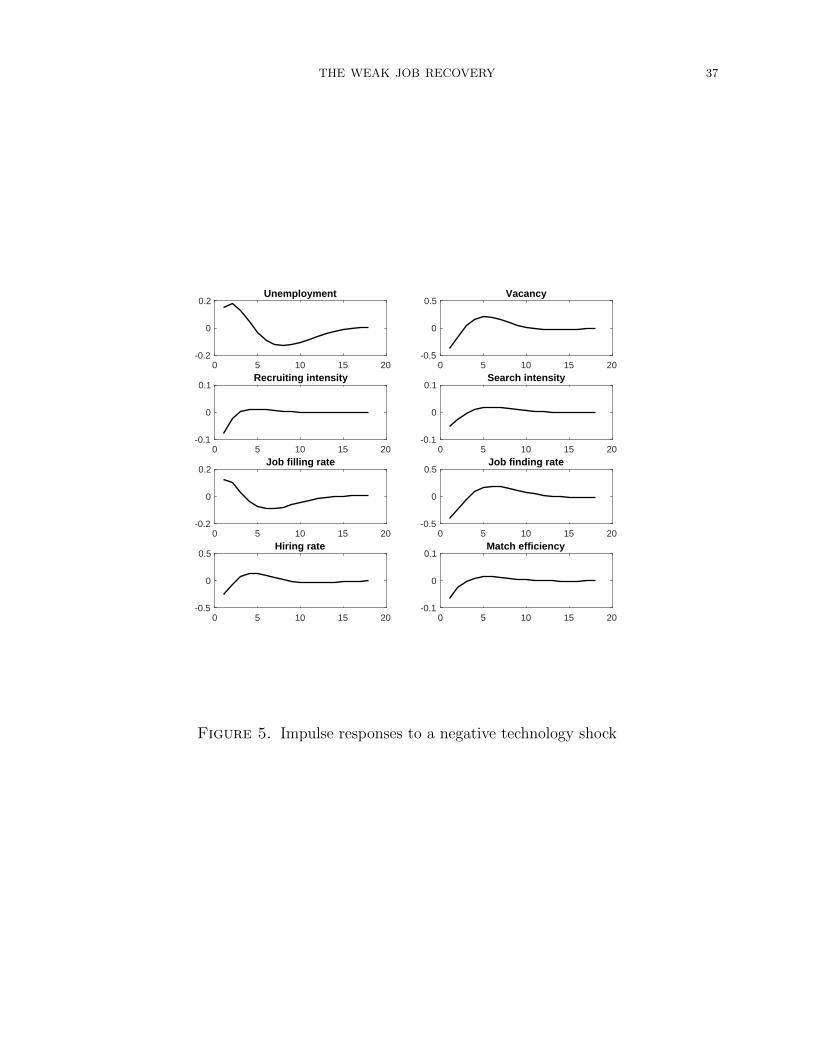
THE WEAK JOB RECOVERY 37
0 5 10 15 20-0.2
0
0.2Unemployment
0 5 10 15 20-0.5
0
0.5Vacancy
0 5 10 15 20-0.1
0
0.1Recruiting intensity
0 5 10 15 20-0.1
0
0.1Search intensity
0 5 10 15 20-0.2
0
0.2Job filling rate
0 5 10 15 20-0.5
0
0.5Job finding rate
0 5 10 15 20-0.5
0
0.5Hiring rate
0 5 10 15 20-0.1
0
0.1Match efficiency
Figure 5. Impulse responses to a negative technology shock
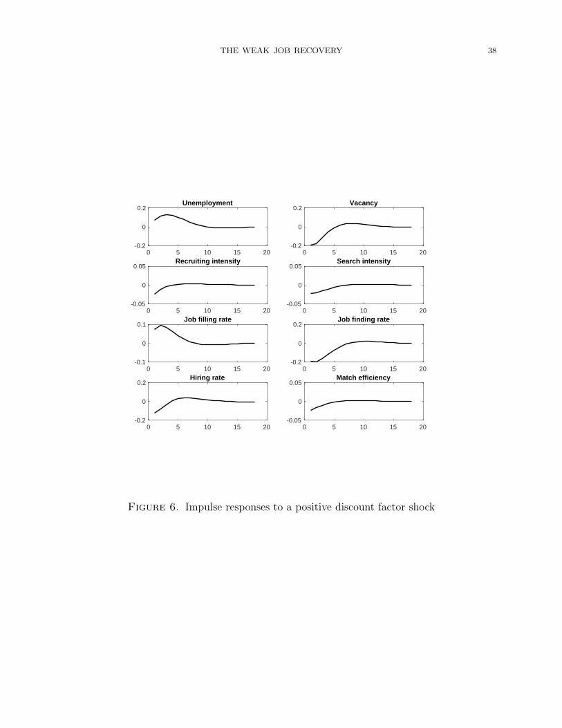
THE WEAK JOB RECOVERY 38
0 5 10 15 20-0.2
0
0.2Unemployment
0 5 10 15 20-0.2
0
0.2Vacancy
0 5 10 15 20-0.05
0
0.05Recruiting intensity
0 5 10 15 20-0.05
0
0.05Search intensity
0 5 10 15 20-0.1
0
0.1Job filling rate
0 5 10 15 20-0.2
0
0.2Job finding rate
0 5 10 15 20-0.2
0
0.2Hiring rate
0 5 10 15 20-0.05
0
0.05Match efficiency
Figure 6. Impulse responses to a positive discount factor shock
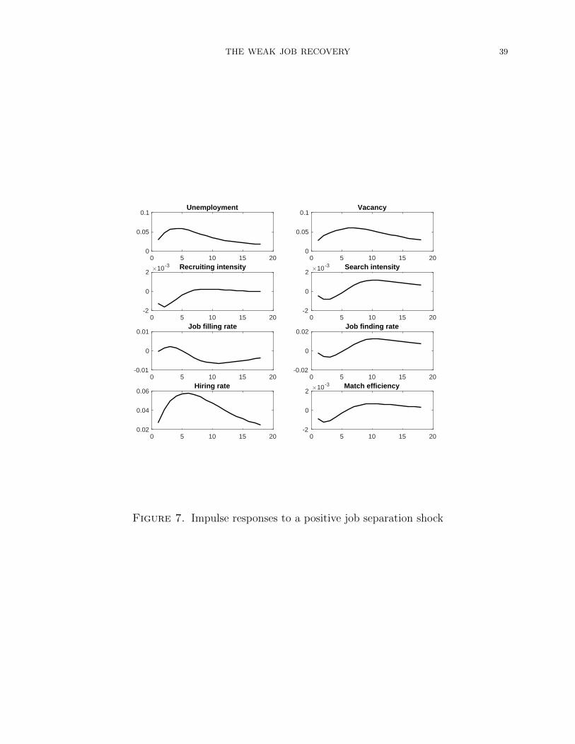
THE WEAK JOB RECOVERY 39
0 5 10 15 200
0.05
0.1Unemployment
0 5 10 15 200
0.05
0.1Vacancy
0 5 10 15 20-2
0
2#10 -3 Recruiting intensity
0 5 10 15 20-2
0
2#10 -3 Search intensity
0 5 10 15 20-0.01
0
0.01Job filling rate
0 5 10 15 20-0.02
0
0.02Job finding rate
0 5 10 15 200.02
0.04
0.06Hiring rate
0 5 10 15 20-2
0
2#10 -3 Match efficiency
Figure 7. Impulse responses to a positive job separation shock
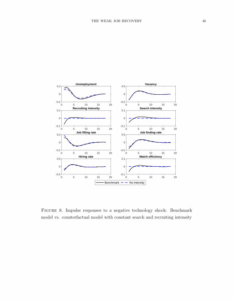
THE WEAK JOB RECOVERY 40
0 5 10 15 20-0.2
0
0.2Unemployment
0 5 10 15 20-0.5
0
0.5Vacancy
0 5 10 15 20-0.1
0
0.1Recruiting intensity
0 5 10 15 20-0.1
0
0.1Search intensity
0 5 10 15 20-0.2
0
0.2Job filling rate
0 5 10 15 20-0.5
0
0.5Job finding rate
0 5 10 15 20-0.5
0
0.5Hiring rate
0 5 10 15 20-0.1
0
0.1Match efficiency
Benchmark No intensity
Figure 8. Impulse responses to a negative technology shock: Benchmark
model vs. counterfactual model with constant search and recruiting intensity
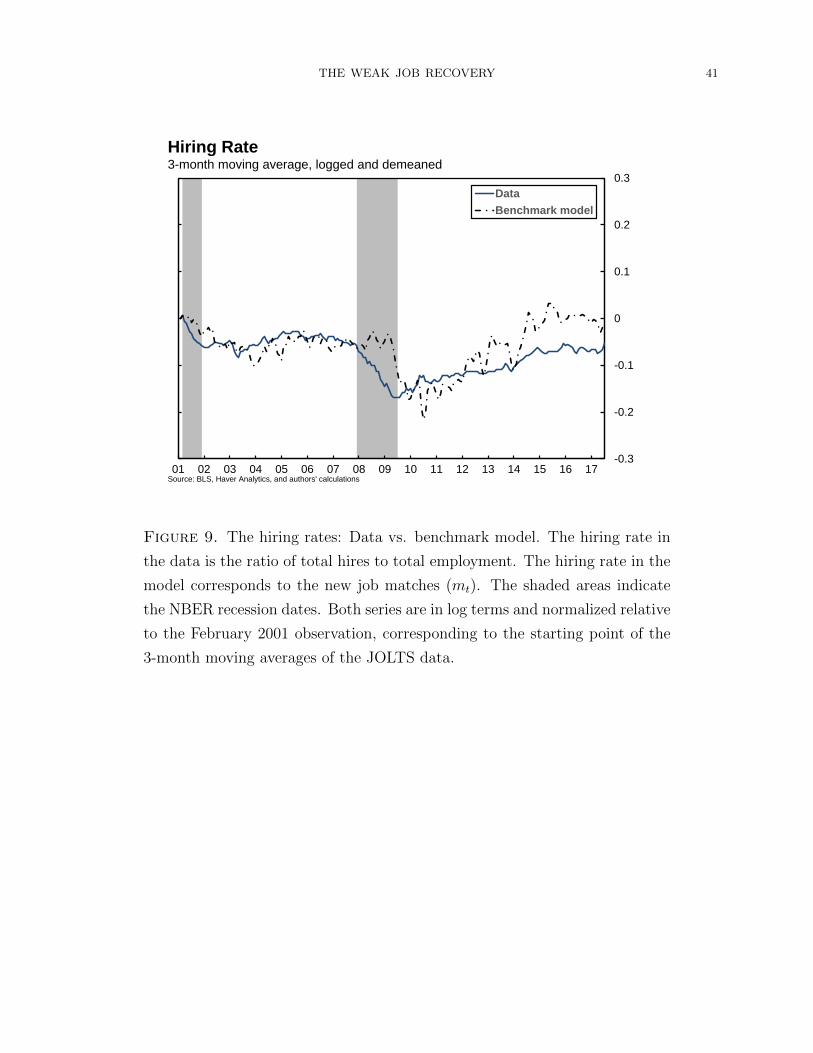
THE WEAK JOB RECOVERY 41
-0.3
-0.2
-0.1
0
0.1
0.2
0.3
01 02 03 04 05 06 07 08 09 10 11 12 13 14 15 16 17
Data
Benchmark model
Source: BLS, Haver Analytics, and authors' calculations
3-month moving average, logged and demeaned
Hiring Rate
Figure 9. The hiring rates: Data vs. benchmark model. The hiring rate in
the data is the ratio of total hires to total employment. The hiring rate in the
model corresponds to the new job matches (mt). The shaded areas indicate
the NBER recession dates. Both series are in log terms and normalized relative
to the February 2001 observation, corresponding to the starting point of the
3-month moving averages of the JOLTS data.
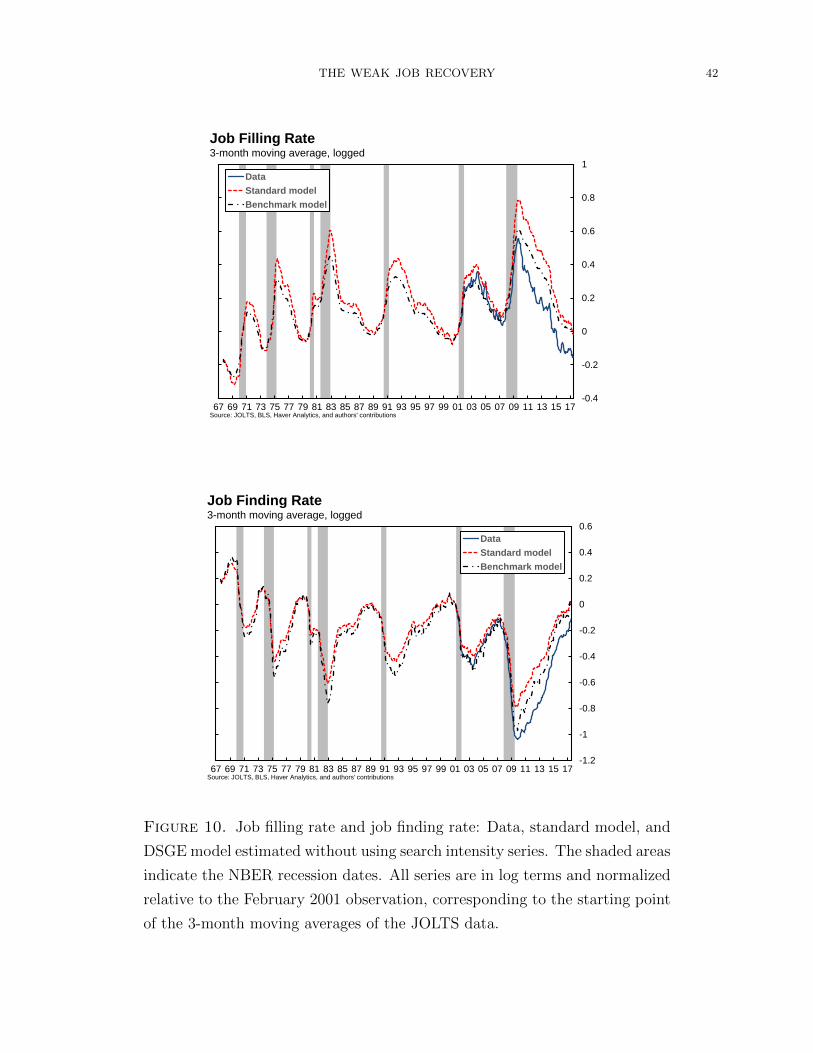
THE WEAK JOB RECOVERY 42
-0.4
-0.2
0
0.2
0.4
0.6
0.8
1
67 69 71 73 75 77 79 81 83 85 87 89 91 93 95 97 99 01 03 05 07 09 11 13 15 17
Data
Standard model
Benchmark model
Source: JOLTS, BLS, Haver Analytics, and authors' contributions
3-month moving average, logged
Job Filling Rate
-1.2
-1
-0.8
-0.6
-0.4
-0.2
0
0.2
0.4
0.6
67 69 71 73 75 77 79 81 83 85 87 89 91 93 95 97 99 01 03 05 07 09 11 13 15 17
Data
Standard model
Benchmark model
Source: JOLTS, BLS, Haver Analytics, and authors' contributions
3-month moving average, logged
Job Finding Rate
Figure 10. Job filling rate and job finding rate: Data, standard model, and
DSGE model estimated without using search intensity series. The shaded areas
indicate the NBER recession dates. All series are in log terms and normalized
relative to the February 2001 observation, corresponding to the starting point
of the 3-month moving averages of the JOLTS data.
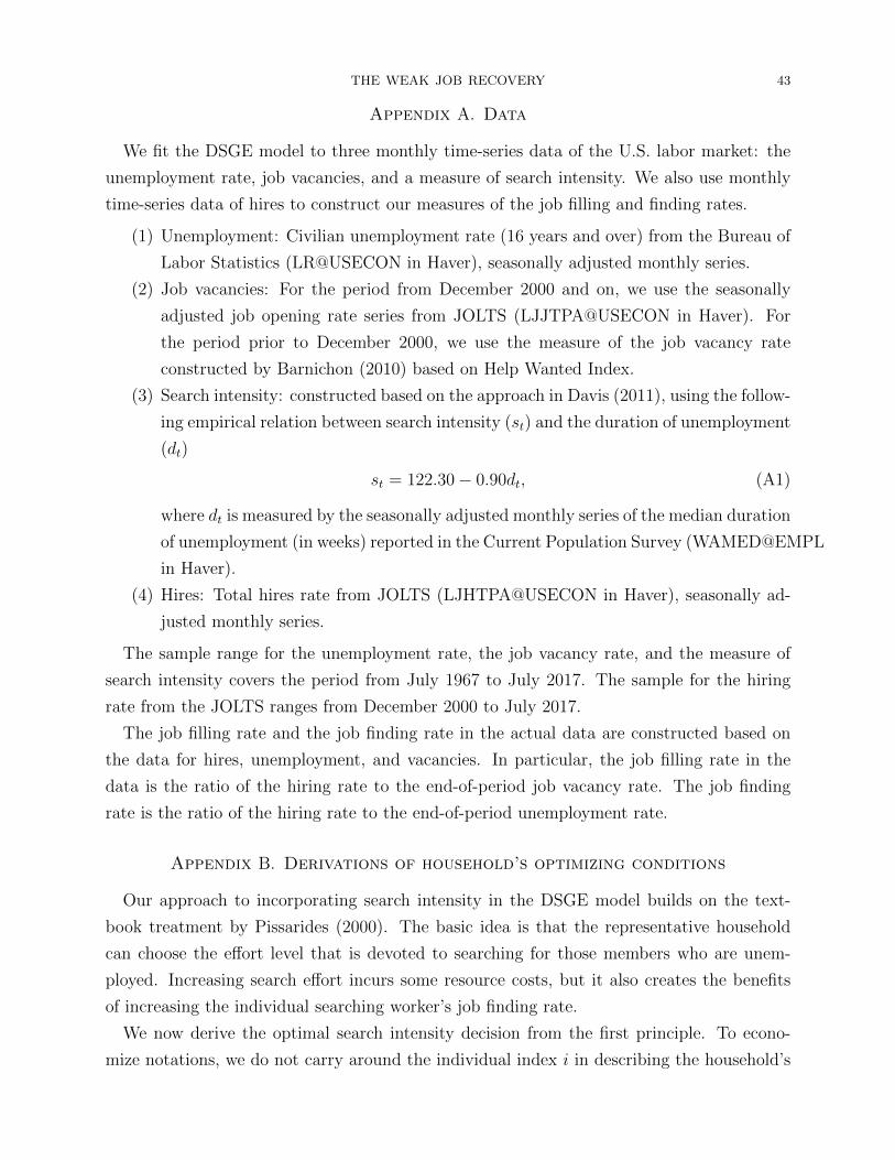
THE WEAK JOB RECOVERY 43
Appendix A. Data
We fit the DSGE model to three monthly time-series data of the U.S. labor market: the
unemployment rate, job vacancies, and a measure of search intensity. We also use monthly
time-series data of hires to construct our measures of the job filling and finding rates.
(1) Unemployment: Civilian unemployment rate (16 years and over) from the Bureau of
Labor Statistics (LR@USECON in Haver), seasonally adjusted monthly series.
(2) Job vacancies: For the period from December 2000 and on, we use the seasonally
adjusted job opening rate series from JOLTS (LJJTPA@USECON in Haver). For
the period prior to December 2000, we use the measure of the job vacancy rate
constructed by Barnichon (2010) based on Help Wanted Index.
(3) Search intensity: constructed based on the approach in Davis (2011), using the follow-
ing empirical relation between search intensity (st) and the duration of unemployment
(dt)
st = 122.30− 0.90dt, (A1)
where dt is measured by the seasonally adjusted monthly series of the median duration
of unemployment (in weeks) reported in the Current Population Survey (WAMED@EMPL
in Haver).
(4) Hires: Total hires rate from JOLTS (LJHTPA@USECON in Haver), seasonally ad-
justed monthly series.
The sample range for the unemployment rate, the job vacancy rate, and the measure of
search intensity covers the period from July 1967 to July 2017. The sample for the hiring
rate from the JOLTS ranges from December 2000 to July 2017.
The job filling rate and the job finding rate in the actual data are constructed based on
the data for hires, unemployment, and vacancies. In particular, the job filling rate in the
data is the ratio of the hiring rate to the end-of-period job vacancy rate. The job finding
rate is the ratio of the hiring rate to the end-of-period unemployment rate.
Appendix B. Derivations of household’s optimizing conditions
Our approach to incorporating search intensity in the DSGE model builds on the text-
book treatment by Pissarides (2000). The basic idea is that the representative household
can choose the effort level that is devoted to searching for those members who are unem-
ployed. Increasing search effort incurs some resource costs, but it also creates the benefits
of increasing the individual searching worker’s job finding rate.
We now derive the optimal search intensity decision from the first principle. To econo-
mize notations, we do not carry around the individual index i in describing the household’s
THE WEAK JOB RECOVERY 44
optimizing problem. Keep in mind that, in choosing the individual search intensity and
employment, the household takes the economy-wide variables as given. In a symmetric
equilibrium, the individual optimal choices coincide with the aggregate optimal choices.
Denote by Vt(Bt−1, Nt−1) the value function for the representative household. The house-
hold’s optimizing problem can be written in the recursive form
Vt(Bt−1, Nt−1) ≡ max lnCt − χNt + βΘtEtVt+1(Bt, Nt), (A2)
where Θt is an exogenous preference shifter. The household’s utility-maximizing decision is
subject to the budget constraint
Ct +Bt
rt= Bt−1 + wtNt + φ(1−Nt)− uth(st) + dt − Tt, (A3)
and the law of motion for employment
Nt = (1− δt)Nt−1 + qu(st)ut, (A4)
where the measure of job seekers is given by
ut = 1− (1− δt)Nt−1. (A5)
The household chooses Ct, Bt, Nt, and st, taking prices and the average job finding rate
as given.
Denote by Λt the Lagrangian multiplier for the budget constraint (A3). The first-order
condition with respect to consumption implies that
Λt =1
Ct. (A6)
The optimizing decision for Bt implies that
Λt
rt= βEtθt+1
∂Vt+1(Bt, Nt)
∂Bt
, (A7)
where θt ≡ Θt
Θt−1denotes the discount factor shock. Combining equation (A7) with the
envelope condition with respect to Bt−1, we obtain the intertemporal Euler equation
1 = Etβθt+1Λt+1
Λt
rt, (A8)
which is equation (17) in the text.
Optimal choice of search intensity st implies that
h′(st) =qutst
[wt − φ−
χtΛt
+ βEtθt+1∂Vt+1(Bt, Nt)
∂Nt
1
Λt
], (A9)
THE WEAK JOB RECOVERY 45
where we have used equation (14) to replace the term ∂qu(st)∂st
byqutst
. The envelope condition
implies that
∂Vt(Bt−1, Nt−1)
∂Nt−1
=
[Λt(wt − φ)− χt + βEtθt+1
∂Vt+1(Bt, Nt)
∂Nt
]∂Nt
∂Nt−1
− Λtht∂ut∂Nt−1
.(A10)
Equations (A4) and (A5) imply that
∂Nt
∂Nt−1
= (1− δt)(1− qu(st)) (A11)
and that∂ut∂Nt−1
= −(1− δt). (A12)
Define the employment surplus (i.e., the value of employment relative to unemployment)
as
SHt =1
Λt
∂Vt(Bt−1, Nt−1)
∂Nt
=1
Λt
∂Vt(Bt−1, Nt−1)
∂Nt−1
∂Nt−1
∂Nt
=1
Λt
∂Vt(Bt−1, Nt−1)
∂Nt−1
1
(1− δt)(1− qu(st)).
(A13)
Thus, SHt is the value for the household to send an additional worker to work in period t.
Then the envelope condition (A10) implies that
SHt = wt − φ−χ
Λt
+ht
1− qut+ Et
βθt+1Λt+1
Λt
(1− δt+1)(1− qut+1)SHt+1. (A14)
The employment surplus SHt derived here corresponds to equation (16) in the text and it is
the relevant surplus for the household in the Nash bargaining problem.
Given the definition of employment surplus in equation (A13), the optimal search intensity
decision (A9) can be rewritten as
h′(st) =qutst
[wt − φ−
χ
Λt
+ Etβθt+1Λt+1
Λt
(1− δt+1)(1− qut+1)SHt+1
]. (A15)
Thus, at the optimum, the marginal cost of search intensity equals the marginal benefit,
where the benefit derives from the increased job finding rate and the net value of employment.
This last equation corresponds to equation (15) in the text.
THE WEAK JOB RECOVERY 46
References
Albuquerque, R., M. Eichenbaum, V. X. Luo, , and S. Rebelo (2016): “Valuation
Risk and Asset Pricing,” The Journal of Finance, 71, 2861–2904.
Barnichon, R. (2010): “Building a Composite Help-Wanted Index,” Economic Letters,
109, 175–178.
Blanchard, O. J. and J. Galı (2010): “Labor Markets and Monetary Policy: A New
Keynesian Model with Unemployment,” American Economic Journal: Macroeconomics,
2, 1–30.
Christensen, B. J., R. Lentz, D. T. Mortensen, G. R. Neumann, and A. Wer-
watz (2005): “On-the-Job Search and the Wage Distribution,” Journal of Labor Econom-
ics, 23, 31–58.
Christiano, L. J., M. Eichenbaum, and M. Trabandt (2015): “Unemployment and
Business Cycles,” Unpublished Working Paper, Northwestern University.
Coles, M. and A. Moghaddasi Kelishomi (2011): “New Business Start-ups and the
Business Cycle,” Centre for Economic Policy Research Discussion Paper 8588.
Cooper, R., J. Haltiwanger, and J. L. Willis (2007): “Search Frictions: Matching
Aggregate and Establishment Observations,” Journal of Monetary Economics, 54(S), 56–
78.
Davis, S. J. (2011): “Comments and Discussion on “Job Search, Emotional Well-Being, and
Job Finding in a Period of Mass Unemployment: Evidence from High-Frequency Longi-
tudinal Data” by Alan B. Krueger and Andreas Mueller,” Brookings Papers on Economic
Activity, 1, 58–70.
Davis, S. J., R. J. Faberman, and J. C. Haltiwanger (2013): “The Establishment-
Level Behavior of Vacancies and Hiring,” Quarterly Journal of Economics, 128, 581–622.
Diamond, P. A. (2013): “Cyclical Unemployment, Structural Unemployment,” NBER
Working Paper 18761.
Elsby, M. W. L., B. Hobijn, A. Sahin, and R. G. Valletta (2011): “The Labor
Market in the Great Recession—An Update to September 2011,” Brookings Papers on
Economic Activity, Fall, 353–384.
Elsby, M. W. L., R. Michaels, and D. Ratner (2015): “The Beveridge Curve: A
Survey,” Journal of Economic Literature, 53, 571–630.
Faberman, R. J. and M. Kudlyak (2016): “The Intensity of Job Search and Search
Duration,” Unpublished Manuscript, Federal Reserve Banks of Chicago and Richmond.
Fujita, S. and G. Ramey (2007): “Job Matching and Propagation,” Journal of Economic
Dynamics & Control, 31, 3671–3698.
THE WEAK JOB RECOVERY 47
Gavazza, A., S. Mongey, and G. L. Violante (2014): “What Shifts the Beveridge
Curve? Recruiting Intensity and Financial Shocks,” Unpublished Manuscript, London
School of Economics and New York University.
Gertler, M. and A. Trigari (2009): “Unemployment Fluctuations with Staggered Nash
Wage Bargaining,” Journal of Political Economy, 117, 38–86.
Gomme, P. and D. Lkhagvasuren (2015): “Worker Search Effort as an Amplification
Mechanism,” Unpubished Manuscript, Concordia University.
Hall, R. E. (2005a): “Employment Fluctuations with Equilibrium Wage Stickiness,”
American Economic Review, 95, 50–65.
——— (2005b): “Employment Fluctuations with Equilibrium Wage Stickiness,” American
Economic Review, 95, 50–65.
——— (2017): “High Discounts and High Unemployment,” American Economic Review,
107, 305–330.
Hall, R. E. and P. R. Milgrom (2008): “The Limited Influence of Unemployment on
the Wage Bargain,” American Economic Review, 98, 1653–1674.
Kaas, L. and P. Kircher (2015): “Efficient Firm Dynamics in a Frictional Labor Market,”
American Economic Review, 105, 3030–3060.
Krueger, A. B. and A. Mueller (2011): “Job Search, Emotional Well-Being, and Job
Finding in a Period of Mass Unemployment: Evidence from High-Frequency Longitudinal
Data,” Brookings Papers on Economic Activity, 1, 1–57.
Kudlyak, M. and F. Schwartzman (2012): “Accounting for Unemployment in the Great
Recession: Nonparticipation Matters,” Federal Reserve Bank of Richmond Working Paper
No. 12-04.
Liu, Z., J. Miao, and T. Zha (2016): “Land Prices and Unemployment,” Journal of
Monetary Economics, 80, 86–105.
Lubik, T. A. (2009): “Estimating a Search and Matching Model of the Aggregate Labor
Market,” Federal Reserve Bank of Richmond Economic Quarterly, 95, 101–120.
Mueller, A. I. (2017): “Separations, Sorting, and Cyclical Unemployment,” American
Economic Review, 107, 2081–2107.
Mukoyama, T., C. Patterson, and A. Sahin (2014): “Job Search Behavior over the
Business Cycle,” Federal Bank of New York Staff Reports No. 689.
Pissarides, C. A. (2000): Equilibrium Unemployment Theory, Cambridge, Massachusetts:
The MIT Press, 2nd ed.
Ravenna, F. and C. E. Walsh (2012): “Screening and Labor Market Flows in a Model
with Heterogeneous Workers,” Journal of Money, Credit and Banking, 44 (Supplement),
31–71.
THE WEAK JOB RECOVERY 48
Rothstein, J. (2011): “Unemployment Insurance and Job Search in the Great Recession,”
Brookings Papers on Economic Activity, Fall, 143–210.
Sedlacek, P. (2014): “Match Efficiency and Firms’ Hiring Standards,” Journal of Mone-
tary Economics, 62, 123–133.
Shimer, R. (2004): “Search Intensity,” Unpublished manuscript, University of Chicago.
——— (2005): “The Cyclical Behavior of Equilibrium Unemployment and Vacancies,”
American Economic Review, 95, 25—49.
Tumen, S. (2014): “Is Search Intensity Countercyclical?” Unpublished Manuscript, Central
Bank of the Republic of Turkey.
Yashiv, E. (2000): “The Determinants of Equilibrium Unemployment,” American Eco-
nomic Review, 90, 1297–1322.