The Wayward Money Supply: APost-Mortem of 1982R. W. HAFER and SCOTT E. HEIN

S INCE the Federal Reserve changed its operatingprocedures in late 1979 to achieve greater control overmonetary aggregate growth, money stock (Ml) growthhas been highly volatile.1 This volatility continuedthrough 1982: Ml grew at annual rates of 1.6.7 percentfrom November 1981 to January 1982, 3.0 percentfrom January to July 1982, and 13.1 percent fronm Julyto December 1982.

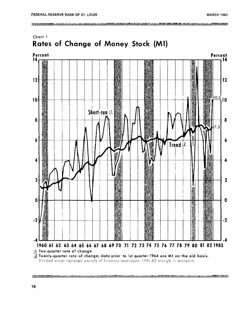
Increased volatility in money growth can produceadverse economic consequences under certain condi-tions. Both economic theory and evidence suggest thatsubstantial short-run deviations in money growth fromits longer-run trend affect the growth of spending andreal economic activity.2 For example, as chart 1 illus-

An earlier cersion of this paper wa.s presented at a Business Ecu-nonmie.s and Pnhlic Policy Workshop at Indiana Unicer.sity. Wewould like to thank all the participants fur helpful conmments,especially Lawrence S. Dacidsurm and Michele Fratianni,

‘For exammmple, the standard deviation of quarterly Nil growth frommmIV/!979 tui IV/1982 is 5.91. In contrast, the standard deviatiomm forNil growth fm’um lV/1976 to 111/1979 was 1.45.

Some may argue that this conmparison is misleading, because tImefluctmmatiuns in recent years likely will flatten umut liver time asevolving seasonal patterns are captured in the recalculation ofseasonal factors, Others, Imowever, have iieen highly skeptical ofrevisinmms in seasonal factors, argniumg that such revisions artificiallysmnooth away outliers. For example, William Poole ammd CharlesLieberman, “Improving Nionetary Control,” Brookings Papers onEconomic Acticity (2:1972), pp. 293—335, have stated that “one ofthe dammgcrs of the X-I 1 model is that uiutliers are all too easilyexplained away by a superficial appeal to chammging seasummals” (p.332).

2This type uifanalysis was presemmted first by Clark \%‘arhurton, “BammkReserves and Business Fluctuations,” Journal of the AmericanStatistical Association (Decemmmlmer 1948), pp. 547—58, reprimmted immClark Warhurton. Depresstun, Inflation, and Monetary Policy:Selected Papers 1945—19,53 (The Johns Hopkins Press, 1966), pp.36—47. Ammalyses in this traditiun also are presented in N’liltonFm’iedmnan and Anna J. Sclmwartz, “Mommey and Business Cycles,”Review of Economics and Statistics (Supplemerut: Fehrnamy 1963),pp. 32—78; William Poole, “The Relationship of Monetary Dcccl-eratiumms to Business Cycle Peaks: Ammother Look at the Evidemmce,”Journal of Finance ~umme1975), pp. 697—712; ammd nmost recentlyNlilton Friedma,m, “Misleading Unanimnity,” N’ewsu’eek (February7, 1983), p. 56.

trates, large negative deviations of money growth fromits trend have been associated with each period ofeconomic decline since 1958.

The increased volatility in money growth has ledmany observers to question whether the Federah Re-serve has the ability to control money growthadequately.3 Some analysts have suggested that theFed must make certain technical changes, such asimplementing contemporaneous reserve accounting,altering discount rate policy and restructuring reserverequirements, to better control the money stock.

This articleexamines whether more stable growth ofthe money stock could have been achieved in 1982without any of the proposed technical changes. To thisend, two simple money stock control procedures areused to simulate money growth in 1982. One proce-dure involves increasing the mnonetary base at a steadyrate. The other involves changing base growth tooffset expected money multiplier changes. The latterprocedure is shown to achieve the hypothetical annualgrowth target with little volatility in quarterly moneygrowth.

tmFur contrasting views on this issue, see Milton Friednmaxm, “l’he

Wayward Money Snppiy,” Newsweek (Decemnber 27, 1982), p. 58;“The Pitfalls of Mechanical Munetarismn,” The Morgan GuarantySurvey (February 1981), pp. 8—13; and Milton Friedman, “Improv-ing Monetary Policy,” Newsweek (July 28. 1980), p. 60. Moresophisticated analyses are presented in Board of Governors of theFederal Reserve System, New Monetary Control Procedures,Federal Resen’e Staff Study, vols, 1 amid 2 (Board uif Governors.198!).

One argumnent is that “large. swings” in the denmand for msmommeyare direct causes of observed variability in money growth. Forexample, see “Statement by Lyle Gramley, memnber, Board ofGovernors ofthe Federal Reserve System, before the Subcommit-tee on Donmestic Monetary Policy umf the House Cummnittee onBanking, Fimmance and Urban Affairs, March 3, 1982,” FederalReserve Bulletin (March 1982), pp. 174-78. Fur an alternativeanalysis, see Scott E. klein, “Short-Run Money Growth Volatility:Evidence of Misbehaving Money Demand?” this Review lJune/July 1982), pp. 27—36; and Kenneth C. Froewiss, “Speaking SoftlyBut Carrying a Big Stick,” Ecunomic Research (Goldman Sachs,December 1982).

17

FEDERAL RESERVE BANK OF ST. LOUIS MARCH 1983

Chart 1

Rates of Change of Money Stock (Ml)

0

12

10

8

6

4

2

0

-2

1960 61 62 63 64 65 66 67 68 69 70 71 72 73 74 75 76 77 78 79 80 81 82 1983[I Two-quarter rate of change.[~Twenty-quarter rate of change; data prior to 1st quarter 1964 are Ml on the old basis.

Shaded- areas represent periods of business recessions. 1981-82 trough is tentative,

12

Percent Percent14 14

8

6

4

2

-2

-4 -4

18

FEDERAL RESERVE BANK OF ST. LOUIS MARCH 1983

Table IMl Growth Rates in 1982

Monthly GE4Wth Rate t~uaderlyi~rowthRate

P etini nary Rev ed amnam’y - Revised181 /82 23V’,~ 25%

1/82 82 34 05

2/82—Z182 a is iv.si 1/82 109%3/82—482 115 184fl582 24 865/82 6/82 03 7 l/82—U/82 353 33

6/82’- 7/82 03 7782 8/82 108 1088/82r 9/82 49 138 11/82—9182 35 6398210/82 226 155

10/82118 183 144 lWS2lV/82 171 139118212/82 92 1142/81 12/82 85 86 IV/81—IV/62 8.5 85

MONEY STOCK GROWI’H iN 1982 the volatility of observed money growth could havebeen considered excessive. Because this present

Table 1 lists Nil growth fbr 1982 on a monthly and analysis addresses the issue of reducing the volatility ofquarterly basis. The respective growth rates are calcu- money growth in an ongoing policy setting, we ignorelated for both preliminary data and the recently re- the reeemmt revisions in money stock numbers; policy-vised data, which incorporate both benchmark revi- makers would not have had this imiformation in 1982sions and revised estimates of seasonal factors. It is when decisions were being made.4

apparent that the recent revisioims have smoothed sub-stantiallv the fluctuations in both monthly and quarter-ly money growth. With the exception of March and ACHIE% INC (;REATER MONEYApril, the revised monthly growth rates all are closer to GROWTH CONTROL IN 1982; TWOthe average growth ratc over the period Thus the U I 1RN Ills I PROC m1fl RI ‘sstandard deviation of the monthly growth rates is re-duced substantially by the revisions: 6.84 vs. 9.59. Could the Fed have achieved a more stable patternSimilarly, the standard deviation of the quarterly of money growth in 1982 than that evidenced by tablegrowth rates is 4.73 for the revised series and 6.62 forthe preliminary series. uThis approach is supported by a recent Federal Reserve Board

report dealing with the problem of seasommal adjustment. In thatreport, it is stated that “since the original projections [of seasonalfactors] are what policymakers and other users of the data have towork with currently in making decisions, the revised data may givean erroneous impression, after the fact, of what the basis for thedecision was.” Board of Governors of the Federal Reserve System,Seasonal Adjustment of the Monetary Aggregates: Report of theCommittee of Experts on Seasonal Adjustment Techniques (Feder-al Reserve Board, 1981), p. 35. Cited in David A. Pierce, “SeasonalAdjustment of the Monetary Aggregates: Summary of the FederalReserve’s Committee Report, “Journal of Business and EconomicStatistics (January 1983), pp. 37—42. Our treatment only addsrealism to the simulations carried out. It does not affect any sub-stantive conclusiomms about comparing alternative operating proce-dures: If revised data are used, the constant-base-growth strategystill results in quarterly money growth volatility in 1982 similar tothat indicated by revised data, but much greater than that associ-ated with the multiplier monitoring approach.

This suggests that at least part of the volatility inmoney growth last year is attributable to poor pre-liminary data. For example, the revised numbers indi-cate that the original estimates of strong money growthin April, October and November all were exaggerated.Similarly, the original estimates of negative moneystock growth in February, May, June and July wereincorrect; the revised data show that money growthwas positive during these months.

The fact that revisions inmoney stock measures havereduced the volatility in money growth is comforting,cx post. For a polieymaker making decisions in 1982,however, the extent of the revisions was unknown and

19

FEDERAL RESERVE BANKOF ST. LOUIS MARCH 1983

1? This question is examined by analyzing two alterna-tive control procedures, each controlling Ml growthby altering the adjusted monetary base (hereafter re-ferred to as base).°

The first procedure involves simply holding thegrowth of the base constant over the year.6 Becausethere generally is a direct relationship betweenchanges in the growth rate of the base and the moneystock, a constant rate of base growth will, on average,yield a predictable growth rate of money. Thisapproach produces stable short-run Ml growth,however, only if the rate of change of the money multi-plier — the connecting link between changes in thebase and money — remains constant over time.Although this typically is the case over longer periodsof time, it is not true over time spans as short as amonth or a quarter. Thus, even though base andmoney growth are closely related overperiods ofa yearor more, short-run money multiplier changes cancause short-run money growth to deviate substantiallyfrom any particular base growth. This is the primaryweakness with this procedure.

The second control procedure alleviates the short-run discrepancies between base arid Ml growth byanticipating changes in the multiplier and, then, offset-ting them by appropriate changes in base growth. This

‘The base is controlled essentially by Fed actions. On the issue ofthe Fed’s ability to control the base, see Anatol B. Balhach, “HowControllable is Money Growth?” this Review (April 1981), pp.3—12.

That study found that “the Federal Reserve can coimtrol themonetary base er-en on a meeek/y basis if it so desires. There is, ofcourse, no question that it can doso over longer periods of time-” Inthis light, no adjustment in achieving a monetan’ base objective ismade. On measuring the base (on an adjusted basis), see R- AltonGilbert, “Revision of time St. Louis Federal Reserve AdjustedMonetary Base,” this Review(Decemher 1980), pp. 3—10; andJohnA. Tatom, “Issues in Measuring An Adjusted Monetary Base,” thisReview (December 1950), pp. 11—29.

°This approach has been advocated in recent statements of the

Shadow Open Market Committee. This is because “[C]urrentinstitutional changes have less effect on the growth of the base thanon most other aggregates.” See “Policy Statement of the ShadowOpen Market Committee, March 16. 1981,” Annual Report. Cen-ter for Research in Govermmment Policy & Business (June 1981), pp.31—35, especially pp. 33-34. This advocacy also is found in theSeptember 14, 1981, “Policy Statement” This argummment presup-poses that stable Ml growth may not be desirable with all of thecurrent institutional changes. In contrast, time present article pre-supposes that stable Ml growth is desirable and seeks to determinethe extent to which it maybe achieved. Of course, the desirabilityofstable money growth depends on the stability ofthe demand formoney, a matter not addressed in this article. For a study that alsorecommends base instead of mnoney stock targeting, see Leonall C,Andersen and Denis S. Karnosky, “Some Considerations in theUse of Monetary Aggregates for the Implementation of MonetaryPolicy,” this Review (September 1977), pp. 2—7.

procedure involves using one-period-ahead multiplierforecasts to determine the extent to which the baseshould be expanded or contracted.’ Two methods offorecasting money multiplier developments are con-sidered for this procedure.

The Constant-Base-Growth Procedure

Analysis of Ml growth and its volatility requireschoosing some desired target level or range. In theanalysis which follows, the top of the announced 1982annual Ml target range —5.5 percent growth — wasselected as a hypothetical operating target.8 Table 2enumerates the desired monthly level of Nil thatwould be consistent with achieving this growth targetwith no short-run variation in Ml growth (see column1). Because the money stock is the product of themultiplier and the base, the growth rate of Ml (Ml) isapproximately equal to the growth rate of the moneymultiplier (iii) plus the growth rate of the base (AMB):

(1) Ml = rh + AMB.

As equation 1 shows, it is necessary to predict th inorder to determine the appropriate AMB to provide.During the last 12 years (1970—Si), the level of themoney multiplier has been declining on average; rim hasaveraged — 1.1 percent. Thus, over this period, basegrowth, on average, exceeded Ml growth by 1.1 per-cent. This was assumed to continue in 1982. To achievethe desired Ml growth of 5.5 percent under the basecontrol procedure considered here, therefore, themoney multiplier is “predicted” to decline at a 1.1percent rate during 1982. Given the assumed rate ofdecline in the money multiplier, a constant 6.6 percentrate of increase in the base would be needed to yieldthe targeted 5.5 percent money growth. This requiredbase path (in levels) is shown in column 3 of table 2.

The constant-base-growth strategy would have re-sulted in stable money growth only if the money multi-plier declined ina steady fashion as presumed. During1982, however, the money multiplier was highly vola-tile by historical standards (see column 2 of table 2).For example, based on original data, the differencebetween the maximum and minimum level of the mul-

A similar argument for using money multiplier forecasts as a basisfor policy actions is presented in Balbach, “How Controllable isMoney Growth?” and James M. Johannes and Robert H. Rasche,“Can the Resem’ves Approach to Monetary Control Really ~Vork?”Journal ofMoney, CreditandBanking(August 1981), pp. 298—313,

81t should he noted that the Federal Open Market Committeetesnporarily ended its practice ofadopting short-run targets for Mlin October 1982, because ofdifficulties in interpreting its behavior,

20

FEDERAL RESERVE BANK OF ST. LOUIS MARCH 1983

Table 2Ml Growth Under Constant 6.6 Percent Base Growth(seasonally adjusted, original data)

Srni.’.ated MI growth rate

Permod Targeted Ml’ Actual multmpmer Smmulatea base’ Smrr’u’alec. Ml Mormthmy Quarterly

B 121 l3~ m2j 511281 2.5951

182 $4429 26142 51708 54465 164%282 4449 25826 17’? 4479 93 78~

382 4468 25809 1726 4455 73482 4488 25837 1736 4485 84582 4509 25566 1745 446’ 62 15

682 4529 25374 ~754 445’ 2.7

782 4549 25354 1764 4472 5.8882 4569 25388 1773 4501 81 4.2982 4590 25598 1782 4562 175

1082 4610 25893 1792 4640 226

1182 4631 26142 1802 4711 191 170

1282 4651 26096 181 1 2726 39

Sm’nuiated Ml growth December ‘981 to Decomoc’r 1982.7 2~

Actual Ml growth Decemnber 1981 to December 1982.8 6’~

Bmllmons of do;.ars

tiplier in 1982 was 0.079. During the past decade thisdifference was exceeded by multiplier developmentsonly during 1974.

Column 4 in table 2 shows the simulated moneystock levels for 1982 holding base growth at a constant6.6 percent throughout 1982, arid assuming that themoney multiplier would have behaved exactly as itdid.9 Two important results emerge from this simula-tion. First, the patterns of both monthly and quarterlyMl growth produced by the constant-base-growthapproach (columns 5 and 6) are similar to those thatactually occurred. Forexample, the verystrong moneygrowth observed in January would have been lessened

‘It miglmt he argued that tIme actual money multiplier pattem’rm wouldhave been considerably different if the Federal Reserve actuallyhad operated under such a control procedure. In tlsis case, theresultammt money gm’owth would have been difierent fromn that re-ported here. This criticismn is predicated on the belief that changesin base growth are assmmciated with changes in the money multi—pher- This belief is not well supported by recent data, however.For example, base growth was relatively stable in 1982, yet moneymultiplier growth was more volatile than any year since 1974.Moreover, for the period 1979 to 1982, the correlation betweenmmmthly base and multiplier growth is amm insignificammt 0.07. Thus,money multiplier nmovements do not appear to he related signifi-cantly to monetary base growth.

only slightly by adopting a constant-base-growthstrategy (23.1-percent vs. 16.4 percent). Nil growthfrom January through July 1982 would have been evenweaker than actually occurred (1.2 percent vs. 0.3percent), and the strong Ml growth from July to De-cember 1982 would have been reduced only slightly(15.1 percent vs. 14.2 percent).

The similarity between actual and simulated Mlgrowth for 1982 is not an aberration; base growth wasindeed fairly stable last year. The volatility in Nigrowth last year was attributable, in large part, tomoney mnultiplier developments, not erratic basegrowth. Thus, those critical of the Fed for the volatilemoney growth last year should recognize that a con-stant-base-growth strategy would not have mnitigatedthis problem.

The second important finding is that Ml growthfrom December 1981 to December 1982 would haveexceeded the hypothetical target by 1.7 percentagepoints if the base had grown at a steady 6.6 percentover the year. The hypothetical growth rate target was5.5 percent; Ml growth would have been about 7.2percent under a policy of constant base growth. This“miss” of the annual Ml target occurred because themoney multiplier essentially was unchanged between

21

FEDERAL RESERVE BANK OF ST. LOUIS MARCH 1983

Table 3MI Growth Using Last Month’s Multiplier as a Forecast of this Month’s Multiplier(seasonally adjusted original data)

Stmulated Ml growth ratePenS Tar9eted Ml Actualmultipher Ommulated be e mrnu ate Ml Month y Quarterty

(1) (2) (3) (4) (5 (6)12/81 2.5951

1/82 $442.9 26142 $1707 $4462 153%2/82 4449 25826 1702 4395 166 70%

38 44&8 25809 1730 4485 209

4/82 4488 25837 173.9 4493 785/82 4509 5566 745 4462 80 31682 4529 25374 1771 4495 927/82 4549 25354 1793 4545 142

8/8 4569 25388 1802 4575 8 92

982 4590 25598 1808 4628 1481082 461.0 25893 1801 468. 95

1162 4631 26142 1789 4676 3 70

12/82 4651 26096 1779 4843 81

Sim’nulated Ml Growth. December 1981 to December 1982 5.

Actual Ml Growth Decembe 961 to December 1982 86%

~Siutonsof dollars

curremmt mommtlm s multiplier plus rammdom ( rrom (p.r)xxlnch c in he a sumcd to he zeto on ax er’ a .:b0

(9\ mmmm — um1

+ p~.

Once the multipl em is fort cast the anmoimnt of h’isemm eded to ‘ichiex the de i ci I “~ I of Nil is thendeterrnirmed m’ siduall Os ‘xanm plc I time mnultiphemis foi e ‘ ist to be 2 60 smext month and the targ 1 for NIltic x nmoimth is .3450 billion the polics directix xx ouldhe to aehiex e ‘i Si 3. 1 billion ($45012.60) im’ise lex cinext mommth. Imm this \ xx muitipli ‘r hanees t~ tIextent that timex are forecast arc ofisc t bx altc immg timebase to mnaintaiim a desu eel path iot NIl. If time mmmiltipile t C ~1 oje cted to he onh 2 50 nc t mnontlm for

vamnple then tim s )roee ciurc xx uicl require $180 bmi—liomm (3430/2.50) in I ‘mc to ‘melmie xc the ai e Ml targc

of $450 billion.

December 1981 and December 1982, instead of de—climmimmg at aim assumed rate of 1.1 percent as it had onaverage ox-er the preceding 10 years. Thus, both the

pattern and average level of money grox’’tlm last yearwere afi’ecteci by unusual money multiplier develop—mclmts, cieveiopnmemmts that would imave had adversennpacts on a constammt—hase—growtlm rule.

MONITORING MONTHLYMULTIPLIER DEVELOPME.NTS

‘I’he previous sectiomm dcrnoimstrates tlmat short—rnmmmommev nmultiplier mnovenments must somnelmow he takeninto aecoummt if more stalmie mnoimev growtim is to heaclmieved. One wax’ to accomplish this is to ohtaimmone—month—ahead incmev multiplier forecasts amid toadjust base growth to offset ilmcreases or decreases 1mmthe multiplier. Two ways of doumg timis are considered.

Na.we Forecast: Monthly Monitoring of timeMnltipiier

The simplest procedure to forecast mmext mommtb’snmonex’ multiplier is to assummie tlmat it will equal the

Table 3 summarizes the results for 1982 using timistechnique to acimieve time same steady 5.5 percentgrowtim rate of Ml as before. Jim comparisomm to theconstant—base—growth strategy, mosmthlv monitoring of

°Scc Ballmaclm . -‘how (2mmmm t rollahle is NI onex’ Groxx’tlm?’’

22

FEDERAL RESERVE BANK OF ST. LOUIS MARCH 1983

mntmltiplier dex’elopments mitigates both proimienms ofexcessive volatility and missing the annual ohjeetix’e.The x•’ariahility imm quarterly Ml growtlm is reduced sub-stantially under the nmuitipher mommitorimmg procedure(compare columnmms 6 1mm tables 2 and 3). 1mm particular,this procedure would not hax’e produced the sharpmidyear slowdown in money growth relative totrendl. The simmiulated mnoney growtlm from 1/1982 to111/1982 ummcler tlmis procedure would imave been 6.4percemmt, suhstammtiailv imigher than the 2.8 percentgrowtlm simnulateel under the constammt—hase—groxx’thstrategy.

Moreover, it also would Imave produced mnom’e stable’quarterly growth imm Ml last year than tlmat simuiateeixvith the constant—base—growth strategy: the standarddeviatiomm of the quarterly growtim rates is 6.76 for theconstant—base—growth strategy- and 2.27 for tIme proce-dure using naive multiplier forecasts. This increasedquarterly stability’ is achiex’ed, imowever, at the ex-pense of slightly’ mnore volatile monthly mnoney growtlm.For example, the standard eleyiatioim of the sinmulatedmonthly Ml growth for the commstammt—hase—growthapproach was 10.21; the figure for the simntmiated Nilgrowth tmsing the multiplier forecast approach was11.27 percent.

The increase 1mm the monthly volatility of Ml growthis a direct commsequence of the procedure itself; timemnommtimlv mnonitorimmg procedure achieves stablequarterly mnonev growth by reactimmg quickly to unex-pected moimthiy disturbances ism the mnoney multiplier.i’hus, wlmemm the mmmuitiplier declimmeei sharply imm May,

this procedure produced a swift policy respoimse immtermns of sharply increased base growtlm imm subsequentmnonths. Consequently, the mimonev stock would hax’ebeen nmuch closer to the hypothetical target level immAugust thamm was the ease with the eommstammt—hase—growtlm strategy.

This simple procedure ofcontrolling Ml growth alsois mnuch mnore successful than the constammt—hasc—groxvtlm strategy imm achieying time desired M 1 growthtarget of5.5 pereemmt. Ml growtlm frommm December 1981to December 1982 would Imave beemm 5.3 pereemit tmeierthis simple multiplier forecasting procedure. commm—pared with a 7.2 percent growth rate under tIme comm—stant—base—growth strategy.

If policy were elirected toward achiex’iog stable quar—ter—to—qmmarter Ml growtim ammd stremmgtimening the Feel’salmilitv to hit an annual target, the simple teelmnique of

mnonetary eomitrol described here xvould he superior tothe constant—hase—gm’owth strategy. It

More Sophisticated Multiplier Forecasts:Time Ser-ies Techniques

The forecastimmg technique described above — usinglast umonths mmiultiplier — is simnpie but ad hoc. Thereis no a priori reason to suspect that sucim a forecastimmgprocedure would he especially reliable. Thus, moresophisticated timne series forecasting models should he

I.-,consmdered. -

Statistical evidence suggests timat omme can miproxeupon the precedimmg forecasting mnodei, wimich mncrelyuses last mnommths multiplier as a prediction for thismonths multiplier. ~ This nprovenmemmt is derived bydeveloping a timne series mnodei that explains changesin the multiplier (i.e., m~— mmmi — ~) by’ using the in—formnation contained in the nomm—ranclomn comnpomment ofthe forecast errors fromn equation 2. More formally, thetime series model cbosemm is represemmtedl by’

(3) mm — rrt1_ = ~ + hm ji.~,

opt, rmmti mm g pm’dmcedlmmu’ previously’ imas I weu simowti to reduce

d1uartd’miy mmm 0mm cv vo]at iiitv-ammdi better aclmicve time loIm g—rm mm I (mimj ec—

tiye i’m 1980 (in Balimaclm, ‘‘lloxv Commtroilah!e is Nionev Growth?”),Si muiiar gaim m s also wom mid have lmeemm adlievedi in 1981 - Basedi (mufim-st—revised data amid! aimu i ug kmr a I )ec’euii5cr 1980 to l)ecm,mmmhcr1981 growl ii rate of 7,0 pem’cemm t. tim is prod’d%lmmme would imave‘-ieidied 7,2 lmerc’mm t simmmtmiate I gm’o~vtim,wi tim the lowest quarterlygrowtim rate hm’im mg 4,5 t’m’c_x’mit anci time im gimest qm marterlv growtimmate heimm g 8. 2 pem-eemm t - Time actual growtim for timis period! wsms 0.4percemmt, xvi tim time qtmam-teriv grov.’th rates rzmmm gimm g frm mm mm 0.5 perecmto 8,9 Pcm’ee mm t -2’the foiiowimmg ammsdvsis (-0mm tim m mmes i mm the trarhit iomm of’ Ecimmard J.Bomuhoff, - Predieti mm g the Ni ouev Nm mmi tipI i d’r:.-\ Case S tudv fimr timeU- S - smmm d time Netim erlam mds, -, iou r,mo I ofMo rme/ a nj Leo mmoomlea ~ mmlv1977), plm. 32-5—4.5: Jammmes M- Joimammmmes amidi Robert H - Basehe.‘‘Predictimmg the NI om 1ev NI u itipher. ‘‘ Iou rim”! of .1.looeta i-mg Lc’o—mmoflmies ~ulv 1979), pp-3

0i—25: J olmau m mes amid Rasdme, ‘‘Cam m the

Reserves Approadm to Niommetary Commtrol Resdiv Wom’k?” amidNI ichele Fromimtm mmmi am md NI mmstapha N_,’ii)! i. ‘ NI ommev Stock Comm tm’ol i mmthe EEC Commmmtries.’’ U eltmcirtm’e/mafthche.s Are/nc (heft 3:1979),Pp 401—2:3,

-m As a first ste mm 1mm smmch ammaivsis. time am mtocorm’eiation of tim i. firstdi!kre mmcc imm time mmmomm e mmimmitipher (mmm

1— um —. m was exau mhm ed fbr

time m~’~ocifamm m mar)’ 1959 tm m i )ed’e mmml Icr t981, For List mm mom m tim’s‘mm u Itiplier tim ime aim elect i xe fhrec-ast oftimis m mmomm tim’s mml mmitipher, theehammge imm time mm nil tilmi icr slmomild mm mt he simm toeor related - A mm v evi-dence of’ an tocmmrm’eismt 0mm smm ggests that timcrc is i mmlo rmuation i mm t liepast ii istmmrv of time mm mml lipiier that commId he used! to i mu mm m’ovm’ the’iorec’ast,

Examum mm mug time an tod’m mrreiatiom m fimmmetiomm of time mm ni lip1icr’s tinoe

series imm dicates timat, 10 r time sam mm pic’ pem-iod Jamm uarv 1 959 to I )m,s—cemmmi mer 1981, time ii vpotimes is tImat en m’m’emmt dmsm mmgcs i mm tim t’ mmm ti I ti —

mmher are imidepemmdIe mt of past elmammges comm he rejected at the 5perdem mt signmi fic’ammc-e level-

23

FEDERAL RESERVE BANK OF ST. LOUIS MARCH 1983

Table 4Ml Growth Using One~Montb-AheadMoney Multiplier ForecastEstimated Mod* m1 tnt ~ 0002 + ~ + 0.196 ~ 1(seasonally adjusted original data)

Smrnufated Mi growth rate

Actual Por~castPermod Targeted Mi mult p5ev muitplier S mutated base Simulated M Monthly Quarterly

(1) () (3) (4 5 (8 (7)2,81 25951

1/82 $44 9 2642 25914 $1709 64468 178 ~

2/82 4449 2/5825 26018 170.6 4406 154

3/82 4668 25609 25856 28 4460 164/82 4488 25837 5798 1740 4495 975/82 4509 25566 2.5809 1 47 4466 78 36682 4529 5374 25594 1769 4490 667/82 4549 5354 2530 791 4541 147

8/82 4569 25380 2384 80.3 4577 190 99~82 4590 2.5698 5359 18 0 4833 1 £0/82 4610 5893 2,5531 lEGS 46 5 11182 463 26142 2,93 79 469 7

12/82 4651 6096 6049 aS 4660 82

Simulated Ml Growth Deesmba lb Oeeembet 1982Actua MI Growth flecember 1981 Ic, becenter 1982 &

tmBmuions ofdollars

where p.~i the error from equation 2. An examination more rehahie model of the multiplier than the naiveof the data revealed that the error in the multiplier model used in the previous section, there is really littleprocess last month (Rn — i) exerted a statistically signifi- substantive difference between the two models. Thecant effect on the change in the multiplier for this naive model (equation 2) suggests that changes imm themonth. Moreover, the analysis indicated the existence multiplier are random disturbances (p.j, while theof a slight negative trend in the data. Using this extra time series model (equation 4) only adds a negativeinformation and estimating the appropriate version of trend term and the impact of last period’s disturbanceequation 3 for the period January 1959 to Decenmher (I’t — 1). Thus, there may well be little difference in the1981 yielded the following results: forecasts.

(4) mm — Wm. m = 0.002 + p.m + 0.196 p.~ m, The results found in table 4 suggest that this isindeed the case. The time-series model given by equa-

where agamn P-t represents the random, unforeseen14 tmon 4 was used to forecast the monthly values of the

mnnovatmon to the multiplier process.multiplier for 1982 by continuously updating the fore-

While, for this sample, eqtmation 4 is statistically a cast to incorporate last month’s money mnultiplier de-velopments. The one-step-ahead money multiplierforecasts are listed in column 3. The table also showstmm

Ali data mime seasoualiy adjtmsted. The estimated stammdam’d errorof the umodcI mx 0 001 IS and the I lmmmmg Box 9 statmstnc 9~2) the amnount of h m.se mnjection (column 4) required eachdistrihtmted as ax’ with 10 degrees of freedom, is 11.53. Because month to achiex’e the hypothetical 5.~percent Mltime reported 9-statistic is evemm less timamm time 30 pereemmt critical growth path ifthe multiplier behaved as the timne seriesxaitme(y’=flSO)thcimxpothtsms of mmmdepemmdcmmt rt.smdu dxc mm model predicted In addition the table hsts the It xci

- - and growth of Ml that would have resulted from theFor further rietamls omm thms aptmroacim to forecasting eeormommmic . .

time series, see C. W, J, Granmger a,me1

Paul Newhold, I”oreeastiug simulated base injections had the multmpImer behavedEconomic Time Series (Aeademmmie Tires

5, 1977). - as it actually’ did (coiummms 5, 6 and 7).

24

FEDERAL RESERVE BANK OF ST. LOUIS MARCH 1983

The simulated money growth developments usingthis procedure are similar to those using the naiveforecast strategy (see table 3). For example, the aver-age monthly Ml growth simulated in table 4 is 5.9percent; the comparable figimre using the naive model(table 3, column 5) is 6.2 percent. The quarterlysimulations are also similar; in particular, the two suc-cessive quarters ofvery weak money growth simulatedunder the constant-base-growth strategy are avoidedby either of these forecasting procedures.

Because the multiplier forecasts derived from thenaive and sophisticated models are not that different,the lessons learned from the naive mnodel results aresupported by the evidence found in table 4 for themore sophisticated model. 15 In particmiiar, this multi-plier forecasting procedure comes closer than theconstant-base-growth strategy to achieving the Imypo-thetical Ml growth target. In addition, quarterly vola-tility in mnoney growth is reduced substantially using

tmmWImile the 1959—SI sample period results indicate sommme statistical

gaimm over time naive model in explaimming ehamges in the mnultiplier,the forecasting experience from 1982 shows that, as a practicalmatter, little wimuld have heen gained from emmmployiog the moresophisticated immodel. This is a limited sample 0mm which to draw,hoxvever, and olme slmmmuld mmot conclude that the simple no—changemodel is equally sufficiemmt in all time periods.

either multiplier forecasting technique.tm6 Thus, ifquarterly money growth fluctuations affect real eco-

nomic activity as suggested earlier, the multiplier fore-casting approach to conducting monetary policyappears superior to the constant-hase-groxvth strategy.

CONCLUSION

Monetary policy actions that utilize a constammt-hase-growth procedure generally will not achieve stableshort-run money growth. A post-mortem of 1982money growth indicates that much of the volatility inmoney growth last year was attributable to moneymultiplier fluctuations, not erratic nionetary basegrowth. Consequently, monetary policy aimed atsmoothing the growth of Ml must anticipate and reactto multiplier movements. Thisarticle shows that eithera naive approach to multiplier predictions or a moresophisticated time series model would have enabledpolicymakers to achieve smoother quarter-to-quarterchanges in Ml by varying time groxvth of the adjustedbase to offset changes in the multiplier.

‘°Foraim earlier analysis ofthis type that reaches similar eonclmmsiomms,see Albert E. Burger, ‘The Relationship Between Monetar Baseamid Money: I-low Closef” this Reeiew (October 1975). pp. 3—S.

-

25