THE VIRGINIA CREEPER TRAIL: AN ANALYSIS OF NET ECONOMIC BENEFITS AND ECONOMIC

IMPACTS OF TRIPS

by

Joshua K. Gill

B.S., The University of Georgia, 2001.

A Thesis Submitted to the Graduate Faculty of The University of Georgia in Partial Fulfillment of the

Requirements for the Degree of

MASTERS OF SCIENCE

ATHENS, GEORGIA

2004

ACKNOWLEDGMENTS

I would like to thank my family and friends for their support, encouragement and belief

in my abilities throughout my graduate career. Without there support I would be lost. I would

like to specifically thank my parents, Kevin and Kathy Gill. Thank you for your never-ending

love and support in all the things I do. As well, thank you for instilling in me the values of hard

work and dedication and for teaching me that the things in life that mean the most are the things

that require the most time and effort.

I would also like to thank Tom and Maryann Buckalew for always being there to listen

and being great friends. Thank you to my committee: John C. Bergstrom, J.M. Bowker, Donald

English, and Jeffery Mullen for providing helpful comments and insight. I would like to

particularly thank John Bergstrom, and J.M. Bowker for their persistence, and patience as I made

my way through the process of developing and defending this thesis.

I would also like to acknowledge and sincerely thank The Virginia Creeper Trail Club,

Virginia Trails, The Virginia Department of Conservation and Recreation, The Virginia

Department of Forestry, The National Park Service, The University of Georgia, Department of

Agricultural and Applied Economics, and The U.S. Forest Service, Region 8 and Southern

Research Station for providing the financial, technical, and logistical support needed to collect

the data upon which this thesis was created. Without the support of these contributors, this thesis

would not have been possible.

ii

TABLE OF CONTENTS

ACKNOWLEDGEMENTS……………………………………………………………………….ii

LIST OF TABLES………………………………………………………………………………...v

LIST OF FIGURES……………………………………………………………………………....vi

Chapter

I INTRODUCTION……………………………………………………………………1

A. Greenways…………………………………………………………………………2 B. Rail Trails………………………………………………………………………….4 C. The Virginia Creeper Trail……………………………………………….………..8 D. Study Objectives…………………………………………………………………10 E. Organization of the Thesis……………………………………………………….11

II THEORITICAL BACKGROUND…………………………………………………..12

A. Consumer Demand Theory and for Market Goods………………………………13 B. Nonmarket Goods and Travel Cost Demand Theory……………………………18 C. Consumer Surplus and Economic Value………………………………………..23 D. Economic Impact Analysis…………………………………………….………..26 E. Multipliers………………………………………………………………………..28 F. Application of Value Measurements to VCT……………………………………30

III EMPIRICAL METHODOLOGY…………………………………………………….32

A. Survey Methodology…………………………………………………………….33 B. Individual Travel Cost Model……………………………………………………37 C. Economic Impacts………………………………………………………………..57

IV RESULTS…………………………………………………………………………….65

A. Sampling Results……………………………………………………….………..65 B. Individual Travel Cost Model…………………………………………………....69 C. Aggregate Net Economic Value…………………………………………………82 D. Economic Impacts……………………………………………………………….84 E. Summary of Results……………………………………………………………..89

V SUMMARY AND CONCLUSIONS……………………………………….……….93

iii

A. Summary…………………………………………………………………………93 B. Policy Implications………………………………………………………………95 C. Study Limitations and Future Research……………………………….……….100

REFERENCES CITED…………………………………………………………………………104 APPENDIX…………………………………………………………………………………….109

A. Survey Instrument……………………………………………………………..110 B. Expenditure Profiles……………………………………………………………117 C. Travel Cost Output…………………………………………………….……….138 D. Significance Tests………………………………………………………………146

iv

LIST OF TABLES 1.1 - Types of Greenways…...…………………………………………………………………….3 1.2 - Intermodal Surface Transportation Efficiency Act Trail Related Programs...………………5 1.3 - Transportation Enhancement Programs….………………………………………………….6 3.1 - Definition of Variables Used to Estimate Demand and Value for VCT Trips …………53 3.2 - The expenditure profile from the nonlocal B survey of VCT users………………………..61 4.1 - Winter visitation, by stratum, of VCT users.….……………………………………………66 4.2 - Summer visitation, by stratum, of VCT users.……..………………………………………67 4.3 - Total visitation and person trips for each VCT user type………………………………….68 4.4 - Descriptive Statistics for local and nonlocal VCT users...…………………………………70 4.5 - Descriptive Statistics for the Truncated Negative Binomial Model.………………….……74 4.6 - Maximum likelihood parameter estimates and standard errors of alternative cost specification models for VCT trips……………………………………………………77 4.7 - Expenditure profile for nonlocal primary VCT day users..……………………….………..85 4.8 - Expenditure profile for nonlocal primary VCT overnight users..………………………….85 4.9 - Expenditure profile for nonlocal nonprimary VCT day users..…………………………….86 4.10 - Expenditure profile for nonlocal nonprimary VCT overnight users...…………………....86 4.11 - Total aggregate recreation expenditures for nonlocal VCT trips………………………....87 4.12 - Direct effects of nonlocal expenditures on VCT trips……………………………………88 4.13 - Total economic impacts of nonlocal expenditures on VCT trips..………………………..88 4.14 - Summary Findings of Net Economic Value for Primary Purpose VCT Trips..….……….90 4.15 - Summary Findings of Total Economic Impact from Primary Purpose Nonlocal Trips……………………………………………………………………………………….91

v

LIST OF FIGURES

1.1 - Map of the Virginia Creeper Trail and Surrounding Area…………………………………..9 2.1 - Utility Maximization Solution in a Two-Commodity Market……………………………...14

2.2 - The Individual Demand Curve……………………………………………………………..17

2.3 - The Flow of Visitor Expenditures to Economic Impacts…………………………………..29

2.4 - Net WTP and Expenditures from Annual Per Person VCT Trips………………………….31

3.1 - Flow Chart of Nonlocal Annual VCT Visits to Annual VCT Trips..………………………59

4.1 - Histogram of Annual Trips to the Virginia Creeper Trail...………………………………..72

vi

Chapter I

INTRODUCTION

Outdoor recreation is a source of exercise, relaxation, and socialization for millions of

Americans. The American Recreation Coalition reported that nine out of ten Americans actively

engage in some form of recreation (American Recreation Coalition 2003). Two popular forms of

outdoor recreation are walking and cycling. The 2002 National Survey of Pedestrian and

Bicyclist Attitudes and Behaviors estimated that 164 million Americans over the age of sixteen

walked, ran, or jogged in the summer of 2002. During the same period, the survey estimated that

57 million Americans over the age of sixteen rode a bicycle at least once (Bureau of

Transportation Statistics 2002).

Pedestrians and cyclists surveyed in the 2002 National Survey of Pedestrian and Bicyclist

Attitudes and Behaviors have strong attitudes and feelings towards recreation. Survey response

indicates many pedestrians and cyclists see recreation as a tool to address some of the social

issues in the United States. The social issues pedestrians and cyclists believe recreation

improves include health, education, parent/child communication, and youth criminal activities

(American Recreation Coalition 2003). Individuals and groups sharing these attitudes are

searching for ways to bring recreation outlets closer to home and improve awareness of these

recreation outlets.

The growing demand for outdoor recreation has led to federal, state, and local

involvement in estimating the economic impacts and benefits of outdoor recreation. There are

many scientific publications estimating the economic impacts of outdoor recreation resources.

Moore, Gitelson, and Graefe (1994) estimated the economic impacts of three different rail trails

located in different geographic regions of the United States. English, Kriesel, Leeworthy and

Wiley (1996) estimated the economic impact of recreation trips to the Florida Keys. English and

Bowker (1996) estimated the economic impact of five different rivers located in differing

geographic regions of the United States. Stoll, Bergstrom, and Jones (1988) estimated the

economic impact of recreational boating on the Texas economy.

The literature estimating the demand for, and net benefits of outdoor recreation is

extensive. Betz, Bergstrom, and Bowker (2003) estimated the demand for a proposed rail trail in

Northeast Georgia. Leeworthy and Bowker (1997) estimated the net economic benefits of

recreation trips to the Florida Keys. Bowker, English, Donovan (1996) estimated the value of

whitewater rafting trips in the Southeast. Siderelis and Moore (1995) estimated the net benefits

of trips to three different rail trails in different regions of the United States. This thesis seeks to

follow the existing literature in estimating the economic impacts and net benefits of trips to the

Virginia Creeper Trail (VCT).

The next section provides background on the origins of the greenway movement and

characteristics of modern greenways. Following this rail trails are introduced. This section

includes a brief history of trail trails and their sources of funding. The Virginia Creeper Trail

(VCT) is then introduced. The section includes a brief history of the area where the trail is

located and the trail itself. The objectives and organization of the thesis conclude the chapter.

Greenways

A greenway is a linear open space established along a natural corridor (Little 1990, p.4).

Greenways are seen in many forms and geographic areas. Greenways are found along

riverfronts, canals, stream valleys, ridgelines, along abandoned railroads, and beside scenic

2

roads. There are five greenway classifications (Little 1990, p.4-5). Table 1.1 lists the five

current greenway classifications.

Table 1.1 – Types of Greenways

1. Greenways created as part of redevelopment programs 2. Recreational greenways based on natural corridors 3. Ecological corridors providing migration, species interchange, and hiking 4. Scenic and historic routes along roads, highways, and waterfronts

5. Comprehensive greenway systems based on landforms, or

combinations of existing greenways

The first greenway was The Park and Piedmont Way on the campus of The University of

California at Berkeley (Little 1990, p.9). The designer, Frederick Law Olmsted went on to

design many other greenways including the Brooklyn-Queens Greenway and the “Emerald

Necklace” in Boston. Other notable figures in the evolution of the greenway movement include

Benton MacKaye and William Whyte. Benton MacKaye established the Appalachian Trail (AT)

as a dam and levee system to combine recreation corridors, and control urban growth (Little

1990, p.19). William Whyte was a landscape architect specializing in open space. His books

included Securing Open Space in America, Cluster Development, and The Last Landscape (Little

1990, p.24).

Beginning in the seventies, citizens and organizations began buying large tracts of green

space along the urban fringe in reaction to urban sprawl (Little 1990, p.32). These “linear

commons” came to be known as greenways. One advantage in developing a greenway was the

decrease in capital needed to purchase land. A long narrow corridor did not hold the private

3

economic value that developers sought and little public funding was available (Little 1990, p.33).

Two important benefits seen from developing greenways are edge and linkage.

Edge is the portion of greenway seen while traveling along the corridor. Edge makes a

relatively small piece of green space appear much larger than it actually is. Edge effect gives a

greenway the effect of having more open space than is actually there. Linkage is the other

defining characteristic of the modern greenway. Greenways provide a corridor for linking

individual recreation resources into a system of parks (Little 1990, p.35-36).

Rail Trails

A rail trail is a greenway established along the right of way of a railway corridor. Rail

trails are a type of natural recreation corridor. This type of greenway is one of the fastest

growing recreation mediums in America. The first rail-trail, The Cathedral Aisle Trail, opened

September 1, 1939 in Aiken, South Carolina (RTC 2003a). Rail trails are well suited for many

popular forms of recreation including, walking, jogging, cycling, rollerblading, and horseback

riding.

Rail-trails are not without controversy, expense, and legal problems. When a railroad

abandons a rail corridor a major issue is who has legal claim to the land. Many previous

landowners feel the land should be returned to them. Landowners argue that since the corridor

was abandoned the right of way should be returned to the previous owner. This has proven to be

a problem in efforts to establish some rail-trails. In recent years the rail banking has gained

popularity as a way to circumvent this problem. Rail banking is a voluntary agreement between

a railroad company and trail agency to use the rail corridor as a trail until the railroad needs the

corridor again for rail service (RTC Railbanking 2003b). Since the right of way is not

abandoned, there is no legal standing for landowners to reacquire ownership of the right of way.

4

Railbanking gained legal standing with the passage of the 1983 National Trails Act (Little 1990,

p.102).

Rail trail conversion was boosted in 1991 with the passage of the Intermodal Surface

Transportation Efficiency Act (ISTEA and Trails 1995). ISTEA officially recognized walking

and bicycling as modes of transportation. ISTEA increased funding for pedestrian and cycling

facilities by incorporating greenway and rail trail projects into state DOT budgets. From 1991

through 1997 approximately $3 billion where earmarked for trail related usage (ISTEA and

Trails 1995). ISTEA has eleven specific trail related programs. Table 1.2 lists trail related

programs supported by ISTEA.

Table 1.2 – Intermodal Surface Transportation Efficiency Act Trail Related Programs

1. Transportation Enhancements 2. National Recreation Trails Fund Act 3. “Core” Surface Transportation Program 4. Congestion Mitigation & Air Quality Improvement

5. Federal Lands Program 6. Scenic Byways

7. Highway Safety 8. Bridge Program 9. National Highways

10. Federal Transit Fund 11. Demonstration Projects

The Transportation Enhancements (TE) program has had the most impact on rail trail

development. This program earmarked 10 percent of all federal transportation dollars to

developing pedestrian and cycling facilities. TE’s provided funding for projects in ten categories

(ISTEA and Trails 1995). Table 1.3 lists the ten projects that are supported by the

Transportation Enhancements program. The categories providing the most benefit to rail-trail

5

conversion are Bicycle & Pedestrian Facilities and Preservation of Abandoned Railway

Corridors (ISTEA and Trails 1995).

Table 1.3 -Transportation Enhancement Programs

1. Bicycle & Pedestrian Facilities 2. Acquisition of Scenic Easements & Historic Sites 3. Scenic or Historic Highway Programs 4. Landscaping & Scenic Beatification 5. Historic Preservation 6. Rehabilitation & Operation of Historic Transportation Facilities 7. Preservation of Abandoned Railway Corridors 8. Control & Removal of Outdoor Advertising 9. Archaeological Planning & Research 10. Mitigation of Water Pollution Due to Highway Runoff

In 1998 ISTEA became the Transportation Equity Act for the 21st Century (TEA 21).

TEA 21 increased TE funding from 10 to 40 percent of federal transportation dollars. TEA 21

also added two more TE programs. Through fiscal year 2002, $6 billion in federal funds have

been earmarked for TE programs. Fifty-four percent of these funds are for rail-trails and cycle

and pedestrian facilities (RTC 2003c). Due to ISTEA, the number of rail trail projects in the

United States has increased. In 1990 there were an estimated 284 rail trails totaling 2,044 miles.

Two years after the passage of ISTEA the estimated number of rail-trails was 655 rail trails

totaling 6,038 miles. The current estimate of U.S. rail trails stands at 1,202 rail trails totaling

12,552 miles (RTC 2003a).

The Federal Highway Administration (FHWA) manages the TE program. The FHWA

annually allocates funding to state DOT’s who handle individual disbursement (RTC 2003c).

For most rail trail projects the state contributes at least 20 percent of the funds and federal TE

dollars account for the remaining 80 percent (RTC 2003c).

6

As rail trails are established local communities have seen the impact that rail-trails can

have on the local economy. Rail trails can help increase land values, strengthen tourism

dependent economic sectors, and create civic pride (Howser 1997). Moore, Gitelson, and Graefe

(1994) demonstrate the economic impact rail-trails have on local economies. Moore, Gitelson,

and Graefe (1994) estimated the economic impact of The Lafayette/Moraga, The Heritage Trail

and The St. Marks Trail on their local economies. Their findings estimate average trail related

expenditures at $3.97, $9.21, and $11.02 per person/per day for The Lafayette/Moraga, The

Heritage Trail, and The St. Marks Trail. This equates to $1.5 million, $1.2 million, and $1.8

million in total economic impact to local economies (Moore, Gitelson, and Graefe 1994).

The rural areas where many rail trails are located were once dependent upon the railroad,

or industries directly related to the railroad as a source of revenue. The creation of the federal

highway system decreased the need for rail transportation and rail lines were eventually

abandoned. Many rural towns lost their economic base. The rail trail movement has helped

some rural towns recover a portion of the revenue lost when rail lines closed. Economic impacts

from rail trail use include increased sales and tax revenue, new business creation, revitalized

business, and increased job opportunities. Rail trails also help to increase tourism, attract

relocating corporations and employees, increased environmental benefits, and increased civic

pride (Howser 1997).

The positive economic impact has bolstered public opinion about rail trails. In the

beginning, many landowners and community members feared rail trails and the people they may

bring in. Many felt that rail trails would create a burden on the community due to increases in

crime and littering from trail users. Instead, it was found that trail users provide a clean source

of revenue that does not require many public services in return. Turco, Gallagher, and Lee

7

(1998) found that the majority of homeowners opposed to trail development changed their minds

within five years, and ten percent of these homeowners sought properties adjacent to the trail.

The Virginia Creeper Trail

The VCT is a 34-mile rail trail in Southwest Virginia, beginning in Abingdon, Virginia

and ending on Whitetop Mountain. The midpoint of the VCT is in Damascus, Virginia. There

are five major trails that intersect in Damascus. These trails are The Appalachian National

Scenic Trail, The Virginia Creeper National Recreation Trail, The Transcontinental Bicycle

Trail, The Iron Mountain Trail, and The Daniel Boone Trail (About Our Town 2002). Damascus

has acquired the moniker, “Trail Town USA.” All or parts of these trails are included in the

Jefferson National Forest and the Mount Rogers National Recreation Area. Figure 1.1 presents a

map of the VCT and surrounding area.

The area experienced significant growth after the Civil War. Many speculators believed

that Southwest Virginia contained large deposits of iron ore. In 1886, J.D. Imboden changed the

name of a small farm community from Mocks Mill to Damascus. Imboden, a wealthy

businessman, organized speculators and created a railroad company to transport the iron ore to

Roanoke (Davis & Morgan 1997, p.47-48). It was soon discovered that the area did not hold the

amount iron ore expected. The iron deposits were soon exhausted and the speculators left. This

allowed for the development of a prosperous timber industry.

Whitetop Mountain held large reserves of virgin timber. In the early 1900’s

entrepreneurs arrived in Damascus to build sawmills, railroads, and furniture operations. With

regular railroad service and large timber reserves, Damascus became a boomtown. During the

Depression the area experienced an economic downturn due to over harvesting and railroad use

began to decline.

8

Figure 1.1 – Map of the Virginia Creeper Trail and Surrounding Area

Railroad use further declined after World War II due to mass appeal of the automobile and a

reduction in area population in search of factory jobs. After fifty years of showing no profit the

railroad corridor was abandoned in 1977 (Davis & Morgan 1997, p.52-66).

Through the coordination of Dr. French Moore, Jr. and Dave Brilhart, M.D, members of

the Abingdon community brought forth the idea of transforming the corridor into a rail trail. The

proposal faced opposition from local landowners wanting the right-of-way returned to the

previous owners. The proposal also faced a time constraint due to plans for the destruction of the

bridges and trestles along the corridor (Davis & Morgan 1997, p.69). With the line abandoned

9

and the insurance policy running out, Norfolk & Western wanted the bridges and trestles

destroyed due to the risk of a large financial loss if someone got hurt. Without the bridges and

trestles the rail trail would be financially impossible.

In 1978 the upper portion of the rail corridor became part of the Mount Rogers National

Recreation Area. Soon after Damascus received funding from the Virginia Commission for

Outdoor Recreation (VCOR) to buy the right-of-way connected to the federal lands. Soon after

the Tennessee Valley Authority (TVA) provided the funding for Abingdon to buy the corridor

connecting Abingdon and Damascus (Davis & Morgan 1997, p.69-70).

The VCT is an interesting mix of public and private partnership. The VCT represents a

unique collaboration between city government, federal government, and local grassroots effort.

Part of this grassroots effort is seen through The Virginia Creeper Trail Club. The Virginia

Creeper Trail Club’s mission is the promotion, maintenance, and preservation of the VCT

corridor (The Virginia Creeper Trail Club 2004).

Study Objectives

The purpose of this thesis is to estimate the economic value and impact of the Virginia

Creeper Trail. Specific questions this thesis will seek to answer include: (1) What is the

economic impact of the VCT on Washington and Grayson counties, and (2) What are the net

economic benefits of trail use to local and nonlocal users. To estimate the economic impact and

net economic benefits of VCT trips the following information is needed:

1. The annual estimated use of the VCT by locals and nonlocals

2. Estimated per person expenditures by nonlocals in the local economy

3. Estimated per person per trip consumer surplus for locals and nonlocals taking a trip to the VCT 4. The demographics of VCT users

10

5. The attitudes and preferences of VCT users with respect to the trail and local area.

Organization of Thesis

This thesis is organized into five chapters. The first chapter provides background

information on rail trails and the VCT. This chapter also defines the research objectives and

purpose of this thesis. Chapter 2 provides the theoretical basis to discuss economic impact and

net economic benefits. Chapter 3 presents the research methodology used to estimate net

economic benefits and economic impacts. This chapter includes the methods used for survey

design, implementation, and sampling. This chapter also discusses the development of the

economic models used. Chapter 4 reports the surveying results and the net economic benefits

and economic impact of trips to the VCT. Chapter 5 discusses the conclusions and limitations of

the research. This section also includes discussion of policy implications for management

decisions regarding rail trails and suggestions for further research.

11

Chapter II

THEORETICAL BACKGROUND

This chapter presents the theoretical concepts necessary to estimate the net economic

benefits and economic impacts of VCT trips. The first section explains the principles of

consumer demand theory, and utility maximization. With this information an individual demand

function is derived. Next, a description of nonmarket goods is given. This section explains why

nonmarket goods are not traded in the marketplace. The theoretical background for the Travel

Cost Method (TCM) and its use for estimating the value of nonmarket goods are given. The next

section defines economic value and how it is measured.

The concepts necessary to perform economic impact analysis are introduced in the next

section. This section identifies the steps necessary to perform economic impact analysis and the

common mistakes made in the application of economic impact analysis. Multipliers and their

role in determining total economic impacts are then introduced. This section explains how

multipliers are used to estimate the induced and indirect effects of expenditures made in the local

economy. The chapter concludes with a section explaining how estimated per person consumer

surplus and estimated per person expenditures are used to estimate the net economic benefits and

total economic impacts of a recreation site like the VCT.

12

Consumer Demand Theory for Market Goods

A rational consumer attempts to maximize utility subject to his/her budget constraint. An

individual’s consumption of private and nonmarket goods reflect this behavior (Freeman 1993,

p.6). The mix of goods and services an individual consumes is referred as their consumption

bundle. A consumption bundle represents the best mix of goods and services the consumer can

consume given their preferences and budget constraint. This consumption bundle represents a

point on the individual’s utility function. The utility function represents an individual’s

preferences among all goods, services, and amenities available (Randall 1981, p.50).

Given the assumption that individuals can rank their preference for various consumption

bundles, the properties of nonsatiation and substitutability emerge. The property of nonsatiation

states that “more is better.” If a consumer is given the choice of two otherwise identical

commodity bundles and bundle A has a larger amount of a normal good X1a than bundle B,

assuming rational behavior, the consumer will always choose bundle A. The property of

substitutability states that within bundle A, if good X1a is decreased then good X2a can be

increased to make the consumer indifferent. The property of substitutability allows for tradeoffs

between goods and services, so that a change in the mix of goods within the consumption bundle

will not change the level of utility the consumption bundle confers (Freeman 1993, p.42). The

properties of nonsatiation and substitutability are shown in Figure 2.1.

In a two-commodity market good X1 represents the good of interest and good X2

represents all other goods within the consumption bundle. The budget constraint, defined by

one’s income, is the downward sloping line from M/p2 to M/p1 denoted as M, with a slope of

– p1/p2. Points along the budget line represent feasible consumption bundles for the consumer.

In Figure 2.1 the utility maximizing solution, given a two-commodity market, is shown as (X*).

13

Figure 2.1 – Utility Maximization Solution in a Two-Commodity Market

X2

M/p2

M

U3

X*

X2a A U2

X2b B U1

M/p1 X1a X1

14

The indifference curves, represented by Ui, i=1,2,3 indicate different utility levels.

Moving outward from the origin, indifference curves represent increasing levels of utility.

Points along an indifference curve represent various combinations of goods X1 and X2 that yield

the same utility. The slope of an indifference curve is called the Marginal Rate of Substitution

(MRS). MRS is the rate at which a consumer will substitute one good for another, with utility

held constant (Varian 1999, p.48).

The properties of nonsatiation and substitutability allow a utility function to represent the

preference ordering of an individual (Freeman 1993, p.43). The utility function is expressed as:

2.1 U = U (xi ,…, xn)

where

U = level of utility

xn = vector of market goods.

subject to a budget constraint:

2.2 m = pixi+ pn xn

where

m = income

pi = market price of good i.

The Marginal Rate of Substitution between good 1 and good 2 is:

2.3 MRS = - 1

2

xx∂∂

| U constant

where

∂x2 = change in good 2

∂x1 = change in good 1.

15

Utility functions are measured on an ordinal scale. Ordinal measurement implies that an

individual can rank his preferences by the amount of utility gained, but these rankings are not

comparable to other individuals (Freeman 1993, p.43).

The point of tangency between the budget constraint and the indifference curve, (X*),

represents the utility maximizing solution. At this point the slope of the budget line, - p1/p2,

equals the MRS. Given the current budget constraint, this point represents the highest utility

possible. If the consumer’s budget constraint changes, the optimal solution would also change.

A decrease in income would shift the budget line inward and an increase in income would shift

the budget line outward. If the price of good 2 and income are held constant while the price of

good 1 changes over different prices, the resulting optimal solutions form the demand curve.

This demand curve expresses the amount of each good the consumer wishes to consume as a

function of the good’s own price, the price of substitute goods, the budget constraint, a quality

measure, and individual characteristics (Freeman 1993, p.99). Figure 2.2 shows an individual

demand curve holding X2, income, substitutes, and individual characteristics constant. At price

P1a, the amount of good X1 demanded is X1a. The ordinary demand function is defined as

(Freeman 1993, p.99):

2.4 Xn = X (pn, ps, m, q, h)

where

pn = price of good n

ps = price of substitute goods

m = income

q = quality measure

h = individual characteristics affecting tastes and preferences.

16

Figure 2.2 – The Individual Demand Curve

P1

A

P1a

Di (X1, P1)

0 X1a X1

17

Nonmarket Goods and Travel Cost Demand Theory

An individual’s consumption bundle consists of private goods, goods provided by the

government, and goods and services from the resource-environment system (Freeman, 1993 p.6).

The private goods that an individual consumes are traded in the marketplace. Private goods

exhibit rival and exclusive characteristics. The goods and services provided by the government

and the resource-environment system are termed nonmarket goods, since they are not traded in

the marketplace. Nonmarket goods cannot be efficiently bought and sold in the marketplace due

to their nonexclusive and/or nonrival characteristics (Randall, 1987 p.175). Goods that exhibit

nonrivalry and/or nonexclusive properties lead to problems with externalities. Externalities

occur when a person’s welfare is not only affected by his actions, but also the actions of a third

party (Randall 1987, p.182). Based on their degree of rivalry and exclusiveness goods can be

classified in four categories (Randall, 1987 p.176).

1. Rival, Exclusive Goods. These goods are bought and sold in the marketplace. Rival, exclusive goods have well-defined property rights allowing for efficient marketplace allocations.

2. Rival, Nonexclusive Goods. These are goods where consumption by a person limits

the amount available for other consumers, but there is no payment method to limit consumption. With well-defined property rights the marketplace could efficiently provide these goods.

3. Nonrival, Exclusive Goods. These are goods that could be provided by both the

public sector and marketplace, but not at a Pareto efficient allocation due to nonrivalry.

4. Nonrival, Nonexclusive Goods. Goods in this category can only be provided by the

public sector. Consumers cannot be excluded and consumption does not limit the ability to use. There is no incentive to buy or sell these goods.

While there are many types of outdoor recreation that are traded in the marketplace some

forms of outdoor recreation are nonmarket goods due to nonrival and/or nonexclusive

characteristics. Nonrival, exclusive types of outdoor recreation are recreation activities where a

18

person’s use of the recreation area does not affect use by another individual, but access to the site

is controlled through points of entry. Examples of nonrival, exclusive recreation resources

include large national parks such as Yellowstone National Park. Recreation sites without

controlled access points or the inability to exclude users not entering at controlled access points

exhibit characteristics of nonrival, nonexclusive goods. Examples of nonrival, nonexclusive

recreation resources include linear greenways where users enter and exit anywhere along the trail

and their use does not affect the use of others.

Recreation resources can be nonrival, nonexclusive to a congestion threshold and then

become rival, nonexclusive. Congestion implies the marginal cost of an additional user is zero to

the point where an additional user creates disutility (Randall 1987, p.176-177). On recreation

sites with no payment method, congestion acts as a mechanism to limit users (Randall 1987,

p.177). Those who value areas with little crowding choose recreation outlets where congestion is

not a problem. The type of characteristics a recreation resource exhibits can be dynamic,

changing due to seasonal variation in use patterns, time of week, and weather.

The VCT has the characteristics of a nonrival, nonexclusive good. Use of the VCT does

not limit use by others and there is no fee for trail use. These characteristics could change if use

continued to increase and congestion became a problem or if fees were charged for trail entry.

Charging for trail use could be problematic due to users ability to enter the trail at points other

than the major access points and due to portions of the trail passing through private property.

The value of a recreational trip derives from the consumer’s desire to maximize utility

from the recreation experience (Stoll 1983). The value of a recreational experience is a function

of market commodities, nonmarket commodities and time (Becker 1965). The following

equations expand on the idea of utility maximization for market commodities, presented in

19

Equations 2.1 and 2.2 and Figure 2.1. Utility maximization of a recreation trip can be expressed

as (Freeman 1993, p. 445):

2.5 max U= U(xn, r, q)

where

xn = vector of market goods

r = annual recreation trips

q = environmental quality index of site j constant for all i consumers

subject to a budget constraint

2.6 m = pnxn + prr

and a time constraint

2.7 t* = tw+(t1+t2)r

where

m = income

pn = vector of prices for market goods

pr = vector of prices for annual recreation trips

t* = total discretionary time

tw = work hours

t1 = round trip travel time

t2 = onsite time

Equation 2.7 shows the opportunity cost of time invested in recreation use. The opportunity cost

of time includes total travel time and total time spent onsite. Since users invest time and money

to use the recreation site, a simple aggregation of expenses does not accurately represent the true

costs of site use (Randall 1981, p.301). The full price of a visit consists of the access fee, the

20

monetary cost of travel, the time cost of travel, and the opportunity cost of time (Freeman 1993

p. 446):

2.8 pr = f + pd*d + pw(t1+t2)

where

f = access fee

pd = monetary cost of travel

d = round trip distance

pw = wage rate

The individual demand function for a recreational trip constrained by income and time is:

2.9 Xr = X(pn, pr, m, t*, q, h)

Outdoor recreation sites have at least two important characteristics that are of economic

importance. First, outdoor recreation confers economic value through site characteristics and

secondly, site access is often a nonmarket good (Freeman 1993 p.443). To measure the value of

a recreation site, a method for approximating the cost of site access is needed. The research

reported in this thesis uses the Travel Cost Method (TCM) to approximate the costs of using a

natural recreation site.

Howard Hotelling first conceptualized TCM in the 1940’s, theorizing that the value of

outdoor recreation could be inferred by the cost of travel and the purchases made while onsite

(Randall 1981, p.300). Clawson and Knetsch first implemented TCM in the 1960’s. TCM theory

implies a tradeoff between travel cost and site access. Travel cost varies among users and sites,

creating the variation necessary to estimate the demand for recreation trips (Freeman 1993

p.444). The variation in trip costs and the weak complimentary relationship between travel cost

and site access allows for estimation of an ordinary demand curve for recreation use (Karasin

21

2004). Weak complimentarity implies that a relationship exists between a market and nonmarket

good such that, when demand for the market good is zero the marginal utility of the nonmarket

good is also zero (Freeman 1993, p.105). The complimentary relationship between travel cost

and site access creates a condition where travel consumer surplus and resource consumer surplus

are equivalent (Hof 1993, p.53).

TCM allows for the construction of an ordinary demand curve where trips demanded are

a function of individual travel costs and other relevant variables. If an ordinary demand curve

can be estimated, then the value of site access can be measured. The measure of this value is net

willingness to pay (WTP), or consumer surplus. Ordinary consumer surplus is estimated by

integrating the ordinary demand curve from the average travel cost to the choke price (Freeman

1993, p.445).

The TCM operates on six assumptions (Freeman 1993, p.447):

1. Individuals will respond to changes in travel costs in the way they would respond to a change in the access fee.

2. Each trip to the site is for the primary purpose site use.

3. All visits entail the same amount of time onsite.

4. There is no utility/disutility derived from time spent traveling to the site.

5. The wage rate represents the opportunity cost of time.

6. There are no alternative recreation sites available.

TCM is not a perfect technique and there remain unresolved questions in the literature

about dealing with these assumptions. One concern is how to deal with multiple purpose trips.

A trip taken for the purpose of visiting more than one site results in joint costs. These joint costs

make it difficult to determine how much value each individual site confers (Freeman 1993,

p.447). There are also unresolved questions surrounding travel to the site. It is assumed that no

22

utility or disutility is derived from travel to the site. When there is utility or disutility from travel

to the site this assumption does not hold (Randall 1981, p.301).

Another important decision when applying a travel cost model is how to measure the

value of time. To account for the opportunity cost of time, it is standard practice to use a fraction

of the wage rate. Application of a fraction of the wage rate to represent the opportunity cost of

time varies throughout the literature. Some researchers use varying wage rates to get a range of

estimates (Zawacki, Marsinko, and Bowker 2000). Other studies have used 1/3 the wage rate as

standard practice (Cesario 1976).

Dealing with the issue of substitute sites remains unresolved in the travel cost literature.

The simple travel cost model assumes there are no other recreation sites available. However,

research has shown that failure to include relevant substitute sites in the demand equation results

in biased consumer surplus estimates (Freeman 1993, p.454). There is no consensus on the

treatment of substitute sites in the travel cost literature.

Consumer Surplus and Economic Value

Economic activity increases the well being of individuals in a society, and individuals are

their own best judge of how well off they are (Freeman 1993, p6). Economists express well-

being as utility. Individuals choose the consumption bundle that maximizes utility, subject to

their budget constraint. The choice of a utility maximizing consumption bundle exhibits the

properties of nonsatiation and substitutability. The property of substitutability is fundamental to

the concept of value. Substitutability allows for trade ratios between goods, revealing the value a

consumer has for goods traded between people or markets. This value is measured by net WTP.

WTP represents the maximum sum of money an individual would be willing to pay rather than

23

do without a good (Freeman 1993, p.43). Figure 2.2 shows gross WTP as the area under the

individual demand curve.

2.10 Gross WTPi = = area a, x( ) 1110

, xdPXDa

i∫ *, xa, 0.

Consumer surplus represents the net WTP for a good, the area under the demand curve and

above the price line (Freeman 1993, p.477). Consumer surplus or net WTP is calculated as gross

WTP minus expenditures. This is shown in Figure 2.2 as the area a, x*, pa.

2.11 Net WTPi (consumer surplus) = = area a, x*, paa

a

pi xpdXPXD

a

∗−∫ 111 ),( a.

By aggregating individual consumer surplus across consumers, the net social benefit of a

good can be estimated (Freeman 1993, p.477). Net social benefit is used in benefit-cost analysis

to determine the most efficient use of scarce resources. This efficiency criterion derives from the

Pareto optimal solution.

A Pareto optimal solution is a solution where no other allocation can make someone

better off without making someone else worse off. It is difficult to find a solution that fits the

Pareto optimal criterion. As a second best alternative, an allocation that represents a potential

Pareto improvement is often sought. A potential Pareto improvement exists when the “winner”

of a policy change could compensate the “loser” and still be as well as before (Loomis 1993,

p.119-121).

The individual demand curve in Figure 2.2 measures ordinary consumer surplus.

Ordinary consumer surplus measures are quantifiable surplus measures based on a constant

marginal utility of income (Freeman 1993, p.46). Measurements of welfare change must be

theoretically appropriate and empirically observable (Bergstrom 1990). While ordinary

consumer surplus measures are easily observed, they are not theoretically exact. Exact welfare

24

changes are measured using Hicksian or compensated consumer surplus measures. Compensated

demand functions show consumption at varying prices with income adjusted to keep utility

constant (Freeman 1993, p.45).

There four types of Hicksian welfare measures: compensating variation (CV), equivalent

variation (EV), compensating surplus (CS), and equivalent surplus (ES). These measures are

preferred to ordinary surplus measures because they uphold the ordinal rankings of utility

functions. The true measure of consumer surplus is the area under the Hicksian or compensated

demand curve and above the price line. Despite potential inaccuracies, it has been standard

practice to use ordinary surplus measures as a proxy for compensated surplus measures. Much

of the literature estimating recreation demand uses ordinary consumer surplus measures as a

proxy for compensated consumer surplus measures. Betz, Bergstrom, and Bowker (2003) used

the ordinary demand curve to estimate demand for a proposed rail-trail in Northeast Georgia.

Fix and Loomis (1997) used ordinary consumer surplus to estimate the economic benefits of

mountain biking at Moab. Siderelis and Moore (1995) also used ordinary consumer surplus to

determine the net economic benefits of The Lafayette/Moraga, The Heritage Trail and The St.

Marks Trail.

Willig (1976) defended the practice of using ordinary surplus measures as a proxy for

compensated surplus measures. Willig showed that when expenditures represent a small portion

of total income using ordinary consumer surplus as a proxy for compensated surplus led to small

approximation errors (Willig 1976). When recreation expenditures represent a fraction of

consumer income and the change in travel cost is small, using Marshallian surplus measures to

approximate Hicksian surplus measures are justified based on Willig’s findings (Freeman 1993

p.61). When compared to expenditures made for rent, food, insurance, transportation, vacation,

25

and tuition expenses, trips to many types of recreation resources represent a fraction of consumer

income. There are some forms of outdoor recreation where Willig’s approximations may not

hold. Examples include big game hunting or fishing trips, mountaineering, and motor sports.

These are recreation activities that require significant expenditures and time to enjoy and using

ordinary consumer surplus estimates, as a proxy for compensated consumer surplus may be

inappropriate.

Economic Impact Analysis

This section examines visitor expenditures and the impact on the local economy.

Nonlocal expenditures are defined as the area, 0, pa, X*, xa in Figure 2.2. One of the objectives

of this thesis is to estimate the economic impact to Washington and Grayson counties of nonlocal

trips to the VCT. Nonlocal expenditures related to recreation use impact the local economy in

the form of increased output, income, and jobs. These increases are quantified by performing

economic impact analysis. Economic impact analysis estimates the changes in regional

economic activity that result from some action, measured as changes in visitor spending, regional

income, and/or employment (Stynes 2004). There are three components necessary to perform

impact analysis:

1. Obtain an accurate number of users and user types.

2. Estimate average spending per person per trip for each user type.

3. Determine the regional multipliers.

Impact analysis can be performed as ex ante or ex post analysis. Ex ante is used when

trying to determine impacts from proposed or hypothetical changes and ex post analysis is used

for projects that currently exist. In ex post analysis impacts are measured as changes in

economic activity resulting from the loss of visitors to the area. This method is frequently used

26

when estimating the impacts of recreation visitors and the impacts they have on the local

economy. In ex post impact analysis it is assumed that visits and expenditures related to

recreation would be lost to the local economy as a result of site closure. If there are other

recreation opportunities within the region that could absorb visitors lost as a result of site closure,

this assumption may not hold. Common mistakes made when performing an impact analysis

include (Stynes 2004):

1. Confusing economic impacts with benefits to users

2. Not clearly defining the action for which impacts are desired

3. Not defining an appropriate impact region and separating "new" dollars from outside the area from local spending

4. Using an inappropriate economic impact model or multipliers

5. Mismatch between spending and visit information

6. Not margining goods that are purchased or otherwise accounting for spending that is

captured by the local region

7. Not isolating tourist spending from local spending

Total economic impact is a combination of direct spending and secondary effects. Direct

spending is the total amount spent by nonlocal visitors in the local economy. The equation for

the direct effect of tourist spending is (Stynes 2004):

2.12 Total Expenditures = Number of Visitors*Average Visitor Expenditure

These expenditures represent the direct economic effect the recreation site has on the local

region. To estimate the total economic impact of visitor spending, a regional economic impact

model is employed. This model produces regional multipliers that estimate the secondary effects

of nonlocal expenditures.

27

Multipliers

The direct impact of visitor expenditure creates a “ripple” effect within the local

economy. Initial nonlocal expenditures stimulate local industries and businesses that supply the

recreation and tourism sectors. This stimulation provides income to employers and employees

that can be spent within the region. These effects related to visitor expenditures are termed

secondary effects. Secondary effects are made up of indirect and induced effects. Indirect

effects are changes in sales, income, or jobs to suppliers of the recreation and tourism sectors

within the region. Induced effects are increased regional sales that result from income earned in

recreation or supply sectors (Stynes 2004). These effects are captured through the use of

multipliers. Multipliers measure how much stimulus a dollars of spending creates within the

economy. For example, if a sales multiplier equals 1.33, every dollar a recreation visitor spends

creates $.33 of indirect and induced effects in the local economy. A multiplier expresses

secondary effects as a ratio of total to direct effects. Multipliers are measured for sales, income,

and employment (Stynes 2004). Figure 2.3 shows the flow of visitor expenditures through the

local economy.

When using multipliers to estimate total economic impact, leakage must be accounted for

before applying multipliers to direct effects. Leakage is the portion of sales that leaves the local

economy to pay for goods and services not produced in the area. This leakage must be accounted

for in order to get an accurate estimate of regional impacts. Only those dollars captured by the

local economy should be used to determine total economic impact. The dollars attributed to a

local economy from visitor spending is determined by the capture rate. The capture rate is the

28

Figure 2.3 - The Flow of Visitor Expenditures to Economic Impacts

Local Economy

Nonlocal Expenditures

Direct Economic Impact

Regional Multiplier

Secondary Effects

Total Economic Impact

Induced Indirect

29

ratio of direct sales to total spending. The rate at which these affects are captured depends on the

amount of money staying in the local economy as final demand. The dollars that are spent to

cover the costs of outside production and transportation immediately leave the economy as

leakage and cannot be considered when determining the total economic impact. Direct effects

are the product of total expenditures and the capture rate (Stynes 2004).

2.13 Direct Effects = Total Expenditures * Capture Rate

These direct effects are combined with multipliers to estimate total economic impact of visitor

expenditures (Stynes 2004):

2.14 Total Economic Impact = Direct Effects * Regional Multipliers

Application of Value Measurements to VCT

In this chapter, the value concept of net WTP or consumer surplus and actual expenditures have

been defined and discussed theoretically. In the case of the VCT, these concepts are summarized

in Figure 2.4. The empirical study described in the next chapter was designed to measure

average net WTP or consumer surplus of trips to the VCT. This average WTP is illustrated in

Figure 2.4 by area a, b, p* divided by average trips (c*) taken at the average cost or price of a trip

(p*). Average net WTP can then be multiplied by total trips to estimate aggregate net WTP or

aggregate net benefits of VCT trips. The empirical study was also designed to measure average

expenditures per VCT trip, illustrated in Figure 2.4 by p** c*(area p*, b, c*, 0) divided by

average trips (c*). Average expenditures per trip can then be multiplied by total trips to estimate

total recreation expenditures. We can then combine the estimate of total recreation analysis with

an economic impact analysis model or technique to estimate the total economic impacts of VCT

recreational expenditures on the local region and economy surrounding the VCT.

30

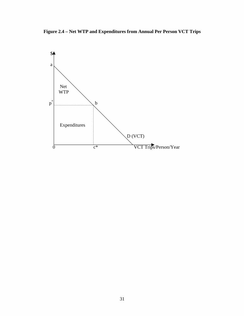
Figure 2.4 – Net WTP and Expenditures from Annual Per Person VCT Trips

$

a Net WTP p* b Expenditures D (VCT) 0 c* VCT Trips/Person/Year

31

Chapter III

EMPIRICAL METHODOLOGY

To estimate the demand, value and impacts of VCT trips a survey instrument is needed to

collect the required information. The first section of this chapter discusses the development and

background of this research project. Included in this section are the goals of the overall research

initiative and the collaborators involved. The next section describes the design, implementation,

collection, entry, and storage of the survey instrument used to estimate net economic benefit and

economic impacts of VCT trips.

Next, the Individual Travel Cost Model used to estimate demand for trips to the VCT is

discussed. Included in this section are advantages and disadvantages of using the ITCM. The

dependent variable and independent variables used in the ITCM are presented. The variables

specified for this model are discussed based on economic theory, and previous trail related

research. The model’s functional form is presented in the next section. This section discusses

the advantages of using count data models for estimating demand from on site surveys. This

section also presents examples of previous research using count data models to estimate demand.

The last section of this chapter focuses on the estimation of economic impacts of VCT

trips. This section presents the expenditure profiles used to determine per person expenditures

made by nonlocals in the impact region. The regional multipliers used to estimate the total

economic impact of VCT trips are also discussed.

32

Survey Methodology

Background

The estimation of net economic benefits and economic impacts of trips to the VCT is

part of a larger project to determine the economic impacts and benefits of trails in the state of

Virginia. The major contributors to this project include; The Virginia Department of

Conservation and Recreation, The Northern Virginia Regional Park Authority, The National

Park Service, The Virginia Trails Association, The U.S. Forest Service and The Virginia

Department of Forestry and The University of Georgia, Department of Agricultural and Applied

Economics. The initial idea was to survey users of all the major trails in Virginia. However, it

was quickly realized that surveying use at every trail in Virginia would be logistically and

financially impossible to complete. To compromise, four representative trails were chosen and

surveys were developed to determine the economic impacts and benefits of each trail. The

representative trails included; The Virginia Creeper Trail, The New River Blueway (NRB), The

Washington and Old Dominion Trail (W&OD), and The Roanoke Valley Greenway System.

The four trails chosen represent four different trail types. The Virginia Creeper Trail is a rural

destination rail trail. The New River Blueway is a water trail. The Washington and Old

Dominion Trail is urban/suburban multi use trail and The Roanoke Valley Greenway System is a

local system of interconnected trails. The first trail surveyed in this research project was the

VCT. Surveying along the NRB and W&OD began a few months later.

Survey Instrument Design

The data collected for this study consisted of trail exit counts and trail user surveys. Trail

counts were obtained using a stratified random sampling approach (Cochran 1977). This is

similar to the methodology used by the USDA Forest Service to estimate visitation in national

33

forests (English, Kocis, Zarnoch, Arnold 2002). An expert panel of locals and nonlocals familiar

with the trail and trail users identified strata. These experts included people from the recreation

retail trade, USDA Forest Service personnel, National Park Service, Virginia Department of

Conservation and Recreation, Virginia Trails, and Virginia Creeper Club members (Bowker

2004).

Three strata were identified season, exit type and day type. Sampling took place in two

seasons. The winter season took place from November through April and the summer season

took place from May through October. High use exits sites and low use exit sites were

identified. The high use exits were Abingdon and Damascus, and the low use exits sites

included Whitetop Station, Green Cove, Creek Junction, Taylor’s Valley, Straight Branch,

Alvarado, and Watagua (Bowker 2004). The third stratum was identified as day type. Sample

days were divided into three day types Saturdays, Sundays/Fridays/Holidays, and non-holiday

weekdays. In the winter season, sampling was done over the complete day. In the summer, days

were segmented into mornings, afternoon, and evening. This was done because of the increase

in daylight hours (Bowker 2004). The winter season contained 1629 total cells in 6 site-day

combinations. With time of day included, the summer season contained 4968 total cells in 6

site-day combinations (Bowker 2004).

Winter Sampling

Winter sampling took place from November 1, 2002 through April 30, 2003. A total of

40 sample days were allocated across the 6 site-day combinations. There were 15 Saturdays, 15

Sunday/Friday/Holidays, and 10 Weekdays selected (Bowker 2004). The sampling dates for

each day type were randomly selected. On a sampling day, trained interviewers were assigned to

34

both high exit sites and to two randomly chosen low exit sites. Interviewers failed to show on

the selected sampling days about 50 percent of the time (Bowker 2004).

A total of 77 site-day combinations were sampled in the winter season. This represents

about 5 percent of the 1629 cells. Coverage for the high exit sites on Saturdays and

Sunday/Friday/Holidays was nearly 25 percent (Bowker 2004). Based on the expert panel’s ex

ante estimate of use, Saturdays and Sunday/Friday/Holidays accounted for more than 80 percent

of total use in the winter season (Bowker 2004). To account for some of the missing days at

Damascus, a proxy count procedure was used. Counts for missing days in Damascus were based

on shuttles sold by one of the local bicycle outfitters and a factor accounting for the outfitter’s

approximate market share (Bowker 2004).

In addition to the exit counts, interviewers administered a survey to individuals exiting

the trail. First, a screener survey (Appendix A - Screener) was used to determine if the trail users

were local (living or working in Washington or Grayson counties) or nonlocal. Other

information the Screener sought included, race, group size, gender, activity mode, and

approximate age. Individuals were also asked if they would be willing to fill out the detailed

survey.

The detailed survey consisted of a local version and two nonlocal versions (Appendix A –

Local, Nonlocal A, Nonlocal B). These surveys were designed to obtain the information needed

to estimate net economic value and economic impacts of the VCT (Bowker 2004). All survey

versions included sections about current trip profile, annual use profile, and household

demographics. The Local and Nonlocal A versions contained questions about personal benefits

from trail use, as well as attitude and preference questions about trail issues, area amenities, trail

35

maintenance, fees, and acceptable use. The Nonlocal B version contained components for trip

related expenditures in the local area and for the entire recreation trip (Bowker 2004).

A pre-test of the survey instrument was done, among the study collaborators, Creeper

Club members, and trail users on Friday and Saturday, September 20-21, 2002. Based on

feedback from this pre-test, the nonlocal survey was broken into two versions in order to keep

survey time to a minimum.

Summer Sampling

Summer sampling followed the same procedure as the winter sampling. Summer

sampling took place from May 1, 2003 through October 31, 2003. A total of 45 sample days

were allocated across the 6 strata. There were 15 Saturdays, 15 Sunday/Friday/Holidays, and 15

Weekdays (Bowker 2004). On a sampling day, trained interviewers were assigned to both high

exit sites and to two randomly chosen low exit sites. The only change from the winter season to

the summer season was the survey periods were divided into three segments, morning, afternoon,

evening (Bowker 2004). These survey periods were randomly selected for each site and day

combination. In the summer season, incidence of interviewers failing to show on the selected

sampling days fell to around 30 percent of the time (Bowker 2004). A total of 107 site-day

combinations were sampled in the summer season. This represents about 2 percent of the 4968

cells.

Coverage for the high-exit sites on Saturdays and Sunday/Friday/Holidays was

approximately 10 percent. Similar to winter, some of the missing days at Damascus was filled

using a proxy count procedure based on shuttle sales and estimated market share. The survey

was administered in the same manner as in the winter season. However, to increase the precision

36

of expenditure estimates for the economic impact portion of the study, the ratio of Nonlocal B to

Nonlocal A surveys distributed was increased (Bowker 2004).

Individual Travel Cost Method

The Individual Travel Cost Model (ITCM) was chosen as the method for estimating net

economic benefits. ITCM estimates individual demand for a recreation site based on individual

travel costs, socioeconomic characteristics, and tastes and preferences. The choice of ITCM was

based on the type of data obtained from the VCT survey, previous trail related literature, and the

merits of ITCM. ITCM has been shown to provide: 1) statistical efficiency in estimation, 2)

theoretical consistency in modeling individual behavior, 3) avoidance of arbitrary zone

definitions, and 4) increased heterogeneity among zonal populations (Bowker and Leeworthy

1998).

There is a precedence of using ITCM in trail literature estimating net economic benefits.

Englin and Shonkwiler (1995) employed ITCM to estimate long run demand for hiking trails in

the Pacific Northwest. Siderelis and Moore (1995) used ITCM to estimate the net benefits of the

Heritage Trail, the St. Marks Historic Railroad Trail, and the Lafayette/Moraga Trail. Fix and

Loomis (1997) used an ITCM to estimate the economic benefits of mountain biking in Moab,

Utah and again in (1998) to compare WTP estimates of mountain biking at Moab using stated

and revealed preference techniques. Betz, Bergstrom, and Bowker (2003) used a variant of the

ITCM to measure demand of a proposed rail trail in Northeast Georgia.

ITCM requires a well-developed survey questionnaire specifically designed to get

individual trip, travel time and distance information. ITCM also requires a significant

investment in time and energy related to surveying, data entry and analysis. However, this was

37

not seen as a limiting problem due to adequate funding, expertise in survey development, a

strong well-coordinated volunteer base, and adequate time for data entry and analysis.

Variable Selection

In order to estimate the net economic benefit of a VCT trip, the appropriate variables

must be specified. Variable specification should be based on economic theory and the previous

literature related to recreation trips using similar modeling techniques. Chapter 2 shows that

ITCM allows for the estimation of an ordinary demand curve where trips demanded are a

function of individual travel costs, substitute prices, income, socioeconomic characteristics, and

tastes and preferences. Following the theory of welfare economics, if an ordinary demand curve

can be estimated, then the value of the site in question can be measured, due to the weak

complimentarity relationship between travel cost and site access. This implies travel consumer

surplus and resource consumer surplus are equivalent, thus allowing for the measurement of

individual consumer surplus for a trip to the VCT. This individual consumer surplus can be

aggregated across users to determine the net economic benefit of the VCT.

Dependent Variable

The dependent variable for the ITCM is the annual number of trips taken to the VCT

(TRIPS). The trail literature is fairly consistent in the way this variable is defined. Betz,

Bergstrom, and Bowker (2003) used average number of annual intended trips to a proposed rail

trail in their trips response model. Fix and Loomis (1997) used annual number of trips to Moab,

minus one, as their trips variable. This was the same variable used in Fix and Loomis (1998).

Siderelis and Moore (1995) used annual number of visits to the Heritage Trail, St. Marks Trail,

and Lafayette/Moraga Trail in their travel cost model.

38

The annual trips question filled out by VCT survey respondents appeared in the VCT

survey as:

aCounting this visit, how many times have you visited the Creeper in the past 30 days? A. 1 B. 2 – 5 C. 6-10 D. 11- 15 E. 16-25 F. 26-35 G. 36-45

H. More than 45

bIncluding this visit, how often have you visited this area to use the Creeper in the last 12 months? ________ times?

a The dependent variable question as it appeared in the local survey. b The dependent variable question as it appeared in the nonlocal surveys.

Locals were asked to report trip behavior on a monthly basis and in categorical form rather than

report a single number. This was done because they were thought to take trips with greater

frequency than nonlocals. Nonlocals were simply asked to report annual number of trips taken to

the VCT.

Since locals were asked about VCT trip behavior on a monthly basis, their responses

needed to be converted to an annual estimate. The first step was to determine the average

number of monthly trips taken by local users. To do this the mid-point for each trip category

was determined; this midpoint was then multiplied by the frequency of trips taken for each

category. These numbers were summed and divided by the total number of people answering the

local trip question to estimate the average number of monthly trips. A significance test was used

to determine whether or not there was a statistical difference between the mean number of local

trips in the winter and summer seasons.

To determine if there was a significant difference between monthly trips in the winter and

summer sampling seasons, a t-test was used. A t-test is a procedure where sample results are

39

used to verify the truth of a null hypothesis (Gujarati 1988, p.109). In this case, the null

hypothesis being tested is that there is no statistical difference in the monthly number of local

trips taken in the winter and summer seasons.

Using the confidence interval associated with the t-statistic, the probability that the t-

statistic lies within the given confidence interval can be estimated for a given significance level.

The t-statistic is the value that comes from the data being tested. This confidence interval takes

the form 100(1- ), where is the significance level. This confidence interval is termed the

“region of acceptance” of the null hypothesis. The endpoints of the confidence interval, the

critical value, establish the “region of rejection” of the null hypothesis (Gujarati 1988, p.109).

The critical value is determined by looking in a t-table. The critical value is based on the chosen

confidence level and the data’s degrees of freedom. A t-statistic that lies outside the “region of

acceptance” is said to be statistically significant.

α α

The t-test performed in this thesis was a two-tailed t-test. In a two-tailed t-test, the two

extreme tails of the probability distribution are considered. In this type of test the null

hypothesis is rejected if the t-statistic lies within either tail (Gujarati 1988, p.111). A two-tailed

test was used because there was no a priori expectation that monthly trips in the two sampling

seasons would change in a specific way. That is there was no expectation that more trips would

be taken in the summer or that less trips would be taken in the winter. A one-tailed t-test would

have been used if there were prior evidence or theoretical expectations that monthly trips would

have changed in a specific way between sampling seasons.

The t-test takes the form (Trochim 2002):

3.1 ∧

⟨

+

−= t

nn

XXt

s

s

w

w

sw

varvar

40

where

t = the t-statistic

wX = mean number of local winter trips

sX = mean number of local summer trips

varw = variance of local winter trips

vars = variance of local summer trips

nw = number of respondents to winter trips question

ns = number of respondents to summer trips question

= the critical value, 1.96 at the 95% significance level ∧

t

The t-test showed no statistical difference in the mean number of trips between the

winter and summer season at the 95% significance level. The t statistic was –1.52 and the

critical value was –1.96. Based on this result, we fail to reject the null hypothesis. This suggest

that there is no significant difference between monthly trips made by locals in the winter and

summer seasons.

The results of the significance test can be found in Appendix D. The final step in

determining the average number of local trips to the VCT was to adjust the number of monthly

trips reported to an annual estimate. This simply involved multiplying the averages for each

response category by twelve.

There was not much information in the literature regarding the conversion of trips from a

monthly basis to an annual basis. Siderelis and Moore (1995) did not mention how they asked

respondents about annual visits to the three rail-trails in their study. In Fix and Loomis (1997)

there was no mention of the format in which they asked about annual trips to Moab, however

based on Moab’s location and its reputation as a major biking destination most users were

41

considered nonlocals. Betz, Bergstrom and Bowker (2003) provided a copy of their trips

question. In their study of intended trips to a rail trail in Northeast Georgia, the annual trips

question was similar to the trips question asked of nonlocal users in the VCT survey.

Independent Variables

Price

Due to nonrival and/or nonexclusive characteristics outdoor recreation on public land is

not traded in the marketplace. There is no traditional market for outdoor recreation and the user

fees for many recreation resources are nominal or zero. Therefore, to estimate an ordinary

demand curve a proxy for price must be developed. The price variable consists of the full price

of a recreation trip made up of the admission fee, the out of pocket cost of travel to the site, the

time costs of travel to the site, and the cost of onsite time (Freeman 1993, p.446).

The literature varies on methods for calculating out of pocket travel costs. Bowker,

English, and Donovan (1996) used reported household expenditures divided by group size plus

the costs of travel, valued at $.092, in their study of guided white water rafting trips. In

Zawacki, Marsinko, and Bowker (2000) two different out of pocket calculations were made in

estimating demand for nonconsumptive wildlife recreation in the U.S. The first model used all

out of pocket expenditures including food, lodging, transportation costs, and fees. The second

model incorporated only out of pocket expenditures for transportation and fees. Fix and Loomis

(1997) chose to only include variable travel and onsite costs in their study of economic benefits

of mountain biking at Moab. Variable travel costs included gas, lodging, airfare, car rental, and

miscellaneous expenses. Onsite costs consisted of lodging, fees, and miscellaneous

expenditures. Fix and Loomis felt that food was not a variable expense and as such was not

reported, nor were durable good expenditures. A similar approach was used in Fix and Loomis

42

(1998) to compare WTP from revealed and stated preference models for mountain biking at

Moab. Siderelis and Moore (1995) applied a measure of direct transportation cost at $.19 per

mile to round trip travel distance to represent out of pocket travel costs in their study of the

Heritage, St. Marks, and Lafayette/Moraga Trails. Betz, Bergstrom and Bowker (2003) used a

similar method for out of pocket travel cost calculation. In their study of demand for a proposed

rail trail in Northeast Georgia, Betz, Bergstrom and Bowker (2003) applied a $.12 per mile

transportation cost to round trip travel distance. Siderelis and Moore (1995) and Betz, Bergstrom

and Bowker (2003) follow the method used by Englin and Shonkwiler (1995) to calculate

recreation demand of hiking trails in the Pacific Northwest.

This thesis follows the logic developed in Englin and Shonkwiler (1995), Siderelis and

Moore (1995), and Betz, Bergstrom and Bowker (2003) for calculating out of pocket costs as

round trip travel distance and direct transportation costs. There is no agreed upon rate at which

transportation costs are measured. Bergstrom, Dorfman, and Loomis (2004) used a value of

$.315 per mile when determining recreational fishing benefits in the Lower Atchafalaya River

Basin in the Gulf Coast region of Louisiana. This higher transportation cost estimate is justified

as the fishermen using this resource were driving larger vehicles and towing boats. Bhat et al.

(1998) used a transportation cost of $.0625 when estimating the value of land and water based

recreation in varying ecoregions in the U.S.

This thesis uses a transportation cost of $.131 to estimate the out of pocket costs of a

recreation trip to the VCT. This cost was reported in the 2003 edition of AAA’s Your Driving

Costs, and represents the average cost for three midsize American vehicles. The average cost

represents the average per mile driving cost for the 2003 model year Chevrolet Cavalier LS, Ford

Taurus SEL, and the Mercury Grand Marquis LS. This cost includes the cost of gas, oil,

43

maintenance, and tires. The transportation cost used in this thesis is within the range of costs

reported by Siderelis and Moore (1995) and Betz, Bergstrom and Bowker (2003) in their

respective rail-trail demand studies. The round trip mileage for each respondent was multiplied

by $0.131 cents per mile to derive the out of pocket travel cost for each trip. Distance traveled

was determined by entering the resident zip code and the zip code of the site where they entered

the VCT into the commercial mapping software package PC MILER 15.0. This produced a one-

way mileage and travel time estimate. To get the round trip mileage and travel time estimate the

one-way estimates were doubled.

It has been shown that the opportunity cost of time is an important part of the cost of a

recreation trip. Failure to include travel time results in biased consumer surplus estimates

(Forster 1989). Since time costs need to be measured in a manner consistent with out of pocket

costs and access fees, a defensible shadow price of time must be used to convert time to a

monetary value (Freeman 1993, p.449). One method for valuing the shadow price of time is to

value time as a function of travel time and an individual’s time value, represented as a fraction of

their wage rate (Betz, Bergstrom, and Bowker 2003). Valuing time costs as a function of the

wage rate and travel time is seen throughout the literature, although there is no consensus on the

appropriate fraction of the wage rate to use. Cesario (1976) valued individual time at one-third

the wage rate in his article estimating benefits of recreation at parks in the Northeast. McConnell

and Strand (1981) use a value of 1/3 the wage rate to measure economic benefits of sportfishing

in the Chesapeake Bay. A time value of 1/3 the wage rate was also used by Bergstrom,

Dorfman, and Loomis (2004) to estimate recreational fishing benefits on Louisiana’s Gulf Coast.

Siderelis and Moore (1995) used a different approach to value time for trips to the

Heritage, St. Marks, and Lafayette/Moraga Trails. Siderelis and Moore (1995) chose to measure

44

forgone income based on wage rates associated with various jobs types. These time costs varied

from 34%, 52%, and 58% on the Moraga/Lafayette, St. Marks, and Heritage respectively. While

one-third the wage rate is commonly used to value time, other studies have used other wage

rates. Bhat et al. (1998) used a time value of one-fourth the wage rate in a study of land and

water recreation throughout various ecoregions in the U.S. Some studies have set as a range of

time values from 0 to ½ the wage rate. An example of this method of time valuation can be seen

in Zawacki, Marsinko, and Bowker (2000). In this study of nonconsumptive wildlife recreation,

the time value was measured at zero time costs, one-fourth the wage rate, and one-half the wage

rate. This logic is also used in Bowker, English, and Donovan (1996) to value guided white

water rafting trips.

While valuing time costs as a function of the wage rate and travel time is used

extensively throughout the literature, some researchers have had difficulty using an arbitrary

portion of the wage rate to determine the value of time. Questions have been raised about the

assumption that individuals freely choose between work and leisure hours based on the wage rate

(Freeman 1993, p.450). In many instances employees are unable to substitute between labor and

leisure hours due to constraints such as the forty hours standard week.

Another concern in valuing time costs is the possibility of utility or disutility from travel,

work, or onsite time. The simple travel cost model assumes there is no utility or disutility from

travel to the site, however if this is not the case then a fraction of the wage rate may be

inappropriate as the shadow price of time (Freeman 1993, p.451). For these reasons Bowker and

Leeworthy (1997) chose to use a binary variable indicating whether or not the individual chose

to forego income to take a trip to the Florida Keys.

45

Other studies treat time as a separate variable. Fix and Loomis (1997) chose to include

time as a separate variable in their study of mountain biking trips to Moab. Fix and Loomis

(1997) chose this method due to the variation in travel time and distance seen in the individual

data used for their study. In the study on demand for a proposed rail-trail in Northeast Georgia,

Betz, Bergstrom and Bowker (2003) excluded travel time because of correlation problems with

travel distance.

This thesis uses two variations on time costs. The first values the opportunity cost of

time at 1/4 the wage rate. Cesario (1976) reported that nonworking travel time should be valued

between one-fourth and one-half the wage rate. The second uses zero opportunity cost of time.

In the second model, only out-of-pocket travel costs are included. This zero time cost estimate

provides a baseline measure of consumer surplus and provides an indication of the importance of

including time costs when estimating benefits of recreation use.

The distance to cost conversion formula is:

3.2 TC = {(TRVLDIST* $.131)+ [(PERWAGE*.25)* PERMILE * TRVLDIST]}

where

TRVLDIST = roundtrip travel distance

PERWAGE = per person wage rate

PERMILE = time per mile traveled

It should be noted that the opportunity cost of onsite time was not included in the model

used in this thesis. Siderelis and Moore (1995) state that travel costs are a necessary input to

produce a rail trail experience and do not contribute to satisfaction gained from onsite trail time.

It is assumed that time on-site is not part of the estimation of user benefits.

46

Substitutes

Theory suggests that inclusion of a substitute variable is important in correctly

estimating the benefits of recreation trips (Loomis and Walsh 1997, p.87-88). The treatment of

substitutes varies throughout the literature. Betz, Bergstrom, and Bowker (2003) used travel

costs for substitute sites based on the origin of the trip in their estimate of demand for a proposed

rail trail in Northeast Georgia. For residents living near metro Atlanta, travel cost for a trip to

the Silver Comet Rail Trail was used. For the remaining sample, travel cost for a trip to a rail

trail in suburban Augusta was used. Fix and Loomis (1997) used price in miles to substitute sites

with characteristics similar to those found at Moab. The first model estimated travel costs to a

site with similar weather patterns and the second model estimated travel costs to a site with

desert conditions. The names of these substitute locations were not given. Zawacki, Marsinko,

and Bowker (2000) used the average cost of a trip from the residence state to another state for

wildlife viewing.

There are also situations where researchers choose not to include a substitute variable.

Englin and Shonkwiler (1995) chose not to include a substitute variable in their estimation of the

long run demand for hiking trails in the Pacific Northwest. In a study of the demand for deer

hunting in California, Creel and Loomis (1990) do not use a substitute variable in their TCM.

This was done because the hunter was not allowed to hunt in another zone once a permit for their

zone of choice was purchased. Siderelis and Moore (1995) also chose not to include a substitute

variable in their study of net benefits associated The Lafayette/Moraga, The Heritage Trail and

The St. Marks Trail. The rail trails studied in Siderelis and Moore (1995) were in different

geographic locations. This resulted in varied substitute availability between the trails studied.

The researchers acknowledge the theoretical importance of substitutes. However, Siderelis and

47

Moore (1995) state their goal was to determine net benefits of rail trails, not trail activities.

Therefore, they considered a substitute site to be another rail trail. In the case of the Heritage

Trail the nearest rail trail was 170 miles away and for the St. Marks Trail the nearest rail trail was

350 miles away. In addition, the survey did not directly seek information regarding recreation

alternatives and the researchers felt that indirect methods for estimating mileage were

inadequate.

Bowker and Leeworthy (1998) used a binary variable to define substitute sites in the

study of user values associated with trips to the Florida Keys. The binary variable in this study

asked whether or not the respondent would travel to an alternative recreation site or participate in

an alternative recreation activity. Bowker, English, and Donovan (1996) used a similar approach

to define substitute sites in a study of the value for guided whitewater rafting trips. Bowker,

English, and Donovan (1996) acknowledge that the choice of a substitute variable remains an

arbitrary decision where it is not always clear if the user is substituting for activity or site

characteristics.

In this thesis, a binary variable was chosen to represent substitutes for recreation

alternatives to the VCT. The VCT surveys asked local and nonlocal respondents whether or not

they felt there was a substitute rail trail for the VCT. A question was also included for nonlocals

that asked the respondent to give the name of the substitute site and the state where it was

located. The question to determine substitute availability filled out by VCT survey respondents

appeared in the VCT survey as:

48

aIn the past 30 days, how many trips have you made to other rail trails like the CREEPER? A. None B. 1 C. 2 – 5 D. 5 – 10 E. 10 – 20 F. More than 20 bIncluding this visit, how often have you visited any other rail trails in the last 12 months? __________ times cBesides the Creeper, what rail trail do you visit most? Name____________ State_______

aThe substitute rail trail question as it appeared in the local survey. bThe substitute rail trail question as it appeared in the nonlocal survey. cThe follow up question asking nonlocals the name and state where the substitute rail trail is located.

Eighty-seven percent of the local population felt there was no available substitute rail

trail for the VCT. Sixty two percent of the nonlocal population felt they had a viable alternative

to the VCT, but less than forty percent of these respondents actually gave the name of that

recreation alternative. Since the substitute question was asked in a different manner to locals and

nonlocals, the substitute variable needed to be changed for use in the model. In this case, the

variables where changed into binary responses. For ease of entry, local responses where entered

by recording each letter as a single digit number starting at one. Therefore, locals who reported

no trips to other rail trails were changed to zero and locals who reported at least one trip to

another rail trail were changed to one. For the nonlocals the respondent indicated the number of

times they visited another rail trail. A nonlocal response of zero was not changed. Nonlocal

responses greater than zero were changed to one. These changes were incorporated into a single

binary substitute variable.

Socioeconomic Characteristics

Socioeconomic variables help to explain the differences in trips demanded by individuals.

Important determinants of demand include income, age, education, race, gender, occupation,

vacation days, hours worked, and region of residence (Loomis and Walsh 1997, p.87-88). The

literature indicates no standard of what should be included in every travel cost model. Englin

and Shonkwiler (1995) used household income, age, gender, and education variables to describe

hikers on Pacific Northwestern trails. Fix and Loomis (1997) only used an age variable in their

49

study of mountain bikers at Moab. Fix and Loomis (1997) found income and skill level to be

insignificant in their model. Zawacki, Marsinko, and Bowker (2000) included socioeconomic

variables describing race, urban characteristics, and age. Betz, Bergstrom, and Bowker (2003)

used before tax household income and an age variable. Siderelis and Moore (1995) included

household income, group size, and two age classification variables, one representing those under

the age of 26 and one representing those over the age of 26.

Non-price variables used in this thesis include, income (INCOME), number in household

using the VCT (NUM), age (AGE), and gender (MALE). Siderelis and Moore (1995) and Fix

and Loomis (1997) found income to be insignificant in determining demand for trail related

activity. However, income was included for theoretical reasons. As discussed in Chapter 2,

commodity demand is based on own price, substitute prices, income, and socioeconomic

characteristics. The amount of household income plays a role in determining the amount of

recreation trips in a household’s consumption bundle. If income increases, the budget constraint

is shifted outward. In this case, if recreation trips are a normal good, trips demanded can be

expected to increase.

The number of individuals in a household who use the VCT could have an effect on the

number trips demanded. Trips to the VCT are costly in terms of both time and money. If more

people in a household use the VCT, then a trip would cost more money. It is expected that larger

households would demand fewer trips. It should be noted that household expenditures were not

included in the travel cost models.

The number of members in a household using the VCT (NUM) was chosen over other

measures of party size. Other party size measures included group size, and spending party size.

NUM was chosen over group size because group size does not necessarily represent those

50

individuals that are in your spending party, particularly when the group size is large. This could

be the case with Boy Scout troops or when people took shuttles and traveled the trail with other

people. Spending party would be a good choice to use in this case. However, spending party

size was only asked for people responding to the nonlocal B questionnaire. Inclusion of

spending party size would have reduced model size to no more than 437.

Although the trail literature was inconclusive on the use of age as a non-price variable,

age was included as a demand determinant for VCT trips. Rail trails have distinct qualities

including long distances, low grades, hard surfaces, straight paths, and the prohibition of

motorized vehicles (Siderelis and Moore 1995). These are qualities that may be attractive to

older outdoor enthusiasts. If rail trails provide qualities that are attractive to older individuals, as

users get older demand for VCT trips would be expected to increase.

A gender variable was also included to determine demand for VCT trips. Loomis and

Walsh (1997) claim gender can be an important demand determinant. The trail literature does

not provide a lot of direction in the inclusion of a gender variable. A variable for gender was not

used in Betz, Bergstrom, and Bowker (2003), Siderelis and Moore (1995), or Fix and Loomis

(1997). Englin and Shonkwiler (1995) included gender to estimate long run demand of hiking.

In Englin and Shonkwiler (1995), if a respondent indicated they were female the likelihood of

trips decreased. If a respondent were female it would be expected that the demand for VCT trips

is lower than trips demanded by male users.

Tastes and Preferences

Individual tastes and preferences can affect demand for recreation trips. Englin and

Shonkwiler (1995) included variables about trail experiences, trail encounters, and a binary

variable describing site characteristics when estimating demand for hiking in the Pacific

51

Northwest. These binary variables included whether or not water was seen on the hike, and if

alpine or grass meadows were present. Creel and Loomis (1990) included length of trip,

number of years hunting a zone, season length, whether a deer was harvested, and the number of

deer that the hunter let walk in the study of deer hunters in California. Bowker, English, and

Donovan (1996) included variables describing previous experience, and onsite time for

whitewater rafting trips. These variables were significant based on their t statistics. Siderelis

and Moore (1995) included a binary variable indicating primary activity. This variable was

mixed in sign and significance depending on the trail in question. Betz, Bergstrom, and Bowker

(2003) included binary variables describing previous experience on rail trails, previous

experience biking, and whether or not the respondent lived in a rural location. Betz, Bergstrom,

and Bowker (2003) thought that users might have different tastes and preferences depending on a

suburban or rural residence. Betz, Bergstrom, and Bowker (2003) found previous experience on

rail trails and biking to be significant and positive in their model. The variable describing

residence was positive, but insignificant.

This thesis included binary variables representing primary trail activity (BIKE) and

people who make over 30 annual VCT trips (HIGHUSE) as taste and preference variables. The

BIKE variable was incorporated to see if biking affected demand for trips. It is not clear whether

or not individual’s whose primary activity is biking will demand fewer or more trips. HIGHUSE

was included in the model to account for those users making more than 30 annual trips to the

VCT. These avid users have a preference for VCT trips that may be significantly different from

other users. Table 3.1 summarizes the variables used to estimate trips to the VCT. The next

section describes the functional form of the model used to determine the demand for trips to the

VCT.

52

Table 3.1 — Definition of Variables Used to Estimate Demand and Value for VCT Trips

Variable Name Definition

TRIPS The annual number of trips taken to the VCT

TC Distance costs and the opportunity cost of time, valued at ¼ the wage rate, for VCT trips.

SUB Binary variable indicating whether or not the respondent felt there was a

viable substitute for the VCT. INCOME Annual household income (1000s) NUM Number of people living in the household that use the VCT AGE Age of respondent MALE Binary variable where male=1 and female=0 BIKE Binary variable for primary activity on the VCT, 1= biking and 0 = other

activities HIGHUSE Binary variable for more than 30 annual VCT trips, 1= trips >30 and 0=

trips < 30

53

Functional Form of the Model

In the current literature associated with recreation demand studies, researchers have

recognized that the dependent variable, i.e., number of annual trips, is a nonnegative integer that

follows a discrete distribution, rather than a continuous distribution (Betz, Bergstrom, and

Bowker 2003). Based on this finding, the preferred modeling technique has been the use of

count data models where the dependent variable is a non-negative number (Blundell, et al. 1995).

Recent studies incorporating count data models include Betz, Bergstrom, and Bowker, 2003;

Zawacki, Marsinko, and Bowker, 2000; Leeworthy and Bowker, 1997; Fix and Loomis, 1997;

Bowker, English, and Donovan, 1996; Englin and Shonkwiler, 1995; Siderelis and Moore, 1995.

Along with improved statistical efficiency, count data models can be corrected for truncation and

endogenous stratification, common problems associated with on-site recreation surveys (Englin

and Shonkwiler 1995 and Betz, Bergstrom, and Bowker 2003).

The data used in this thesis was collected using on stratified random on-site survey. Data

collected in this manner commonly suffer from truncation and endogenous stratification.

Truncation occurs when the sampled population does not include non-users. Endogenous

stratification results due to the higher probability of sampling someone taking frequent trips

(Englin and Shonkwiler 1995). Studies have shown that when count data models are corrected

for truncation and endogenous stratification, the total use value of a recreation site to the whole

user population can be estimated from on-site data (Englin and Shonkwiler 1995).

Two distribution functions are typically used when employing count data models,

Poisson and Negative Binomial. A Poisson distribution gives a probability of “the number of

event occurrences and the Poisson parameter corresponding to the expected number of

54

occurrences is modeled as a function of the explanatory variables” (Kennedy 1998, p. 236).

Estimation using this technique requires maximum likelihood estimation. The probability

function of a Poisson random variable (Y) is defined as:

3.3 !

)(y

eyYfyλλ−

==

where

λ = both the conditional mean and variance of Y.

Parameter λ can in turn be parameterized as (Kennedy 1998, p.237):

3.4 )exp( βλ x=

The Poisson model assumes a constant probability of occurrence at any point in time and the

variance of the number of occurrences are equal to the expected number of occurrences

(Kennedy 1998 p. 237). Stated another way, it is assumed the conditional mean of (Y) equals its

conditional variance:

3.5 [ ] [ ] ( )iiiiii xxyVarxyE βλ exp|| ===

In practice, the assumption of conditional variance equal to conditional mean can prove

restrictive because of overdispersion problems. Overdispersion is a form of heteroscedasticity

where the dependent variable’s conditional variance is greater than the conditional mean,

implying a variance-mean ratio greater than unity (Creel and Loomis 1990). One-way to correct

for this problem is to introduce an error term ( ) that has a gamma distribution (Kennedy 1998

p. 247). A gamma distribution is used for continuous random variables constrained to be greater

or equal to 0, characterized by parameters of shape and scale (University of Florence,

Department of Statistics 2004). This allows the conditional mean and variance to differ, leading

ε

55

to a Negative Binomial Distribution. Under the Negative Binomial conditions (Kennedy 1998 p.

248): the

3.6 mean = λ

3.7 variance = 2

1λαλ −+

where

= the common parameter of the gamma distribution α

Since the negative binomial is an extension of the Poisson distribution it can be expressed

similarly to the Poisson in 3.4.

The survey process used in this thesis leads to data that are truncated at zero. To account

for this problem a truncated negative binomial was chosen to estimate the quantity of trips

demanded to the VCT. Endogenous stratification was not corrected for in the truncated negative

binomial models used in this thesis. Recent studies have shown that adjustment for endogenous

stratification does not significantly improve welfare estimates Ovaskainen, Mikkola, and Pouta

(2001). In their study of recreation trips to Finnish forest recreation sites, Ovaskainen, Mikkola,

and Pouta (2001) found that differences in estimated consumer surplus were small between

Negative Binomial Models accounting for endogenous stratification and those that did not.

(Ovaskainen, Mikkola, and Pouta 2001) estimated consumer surplus when accounting for

endogenous stratification to be $14-14.40 per trip. The estimated consumer surplus when

endogenous stratification was not accounted for was $13.20-13.40 per trip.

The full model of VCT demand is a semi-logarithmic function:

3.8 i

i

uMALEBIKENUMAGEHIGHUSEINCOMESUBTCTRIPS

+++++++++=

876

543210lnβββ

ββββββ

56

Economic Impacts

In this section the methodology used to estimate the economic impacts of nonlocal trips

to the VCT are discussed. The first section offers a discussion of the theory of visitor

expenditures. This is followed by the information from the dataset used to determine economic

impacts. Following this the model used to determine economic impacts will be discussed. After

this an explanation of the conversion of visitors to per person trips used in the impact analysis is

discussed. The last section discusses the use of regional multipliers to estimate total economic

impacts.

The previous sections of this chapter have examined the dataset and model used to

estimate individual consumer surplus for a trip to the VCT. This section focuses on the impact

that nonlocal trip expenditures to the VCT have on the local economy. When individuals use a

recreation site, the local economy derives benefit from the expenditures made as a result of that

trip. These expenditures impact the local economy in the form of increased output sales, income,

and jobs (Stynes 2004). These expenditures are represented by the rectangle box in Figure 2,

defined as the area 0,pa,X*,xa. Individual expenditures can be quantified through economic

impact analysis. Using economic impact analysis, the total economic impact attributed to

recreation use on a local economy can be estimated. An economic impact analysis measures

the amount of dollars brought into the economy by individuals that do not reside in the region of

impact being studied. There were six steps used to perform the economic impact analysis in this

thesis (Stynes 2004): Estimate Use, Estimate nonlocal per person recreation expenditures per

major spending categories, Define local impact region, Estimate aggregate recreation

57

expenditures by user type, Estimate direct effects by user type using the capture rate, and Apply

multipliers to estimate the total economic impact

Visitor use was estimated based on the stratified random sample, developed by J.M.

Bowker, U.S. Forest Service. This sample was described earlier in the chapter. The use estimate

based on the stratified random sample gave an estimate of the annual number of visits taken to

the VCT. In order to estimate economic impacts this estimate was converted to person trips.

Figure 3.1 shows a flow chart describing the conversion of visits to person trips. First, each

respondent was classified as local or nonlocal. To determined if a respondent was local or

nonlocal, respondents were asked if they lived or worked in Washington or Grayson counties.

Based on the answer to the local, nonlocal question, the percentage of local and nonlocal

respondents was determined. Next, the mean number of annual trips and mean number of visits

per trip per user type was determined. These were questions asked on each survey administered.

Mean annual trips and mean visits per trip were multiplied to estimate mean visits per year.

Mean visits per year were multiplied by each nonlocal user type to estimate sample visits per

year. These nonlocal user types will be discussed in more detail in the next section. The sample

visits per nonlocal user type were aggregated to get total sample visits per year. Each sample

visit per nonlocal user type was divided by the total sample visits per year to estimate each user

type’s share of sample visits. The sample visit share for each nonlocal user type was multiplied

by annual number of nonlocal visits to estimate annual number of visits per user type. The

annual number of nonlocal visits was calculated from the use estimate. Annual visits per

nonlocal user type were divided by the mean number of visits per trip per user type to estimate

annual trips per user type. The annual trips per user type were aggregated to get annual person

trips.

58

Figure 3.1 – Flow Chart of Nonlocal Annual VCT Visits to Annual VCT Trips

Mean trips/yr calculated from questionnaire

Mean visits/trip calculated from questionnaire

Mean visits per year (Trips per yr*Visits per trip)

Screener identifies each respondent as local or

nonlocal and gives percentage of local and

nonlocal users

Sample visit shares (Sample visits per yr/Sum of sample visits per yr)

Annual trips per user type (Annual visits/Visits per trip)

Annual visits per user type (Sample visit share*Nonlocal visits)

Sample visits per year per user type (Nonlocal visitor type*Visits per yr per visitor type)

59

The expenditures of importance in an economic impact analysis are nonlocal

expenditures. Nonlocal expenditures represent “new” money being brought into the local

economy. Only nonlocal expenditures are used in the impact analysis because the interest is in

the impact that “new” money has on the local economy. To estimate nonlocal expenditures,

expenditures made by nonlocals in the local economy, based on major expenditure categories

were recorded.

Table 3.2 shows the expenditure profile used in the survey instrument. The major

expenditure categories included; private lodging, public lodging, food consumed in a restaurant

or bar, food consumed outside of a restaurant or bar, primary transportation, other transportation

expenditures, bicycle rentals, shuttle or guide service, entry fees, and other expenditures. VCT

users were classified by user type. The four user types identified at the VCT were primary day

users, nonprimary day users, primary overnight users, and nonprimary overnight users. A

primary user is defined as a user who is in the impact region for the primary purpose of visiting

the VCT. A nonprimary user is defined as a person in the impact region for another purpose, but

chose to spend a portion of time on the VCT.

Based on these nonlocal user classifications, expenditure profiles were developed

describing these user classifications in detail. These profiles contained the average per person

expenditure made in each of the expenditure categories by each user type. These profiles

estimated average expenditures for the entire trip and for expenditures made within twenty-five

miles of the VCT. To get per person expenditures each expenditure category was divided by the

average spending party size in each user classification. A copy of each expenditure profile is

provided in the Appendix B.

60

Table 3.2 - The expenditure profile from the nonlocal B survey of VCT users

A. Spending by your party B. Spending by your within 25 miles of party for the whole

Creeper Trail trip Lodging: Privately owned (motel, cottage, bed & breakfast) _______ _______ Publicly owned (state or FS campgrounds) _______ _______ Food & Beverage:

Food and drinks consumed at restaurants or bars _______ _______ Other food and drinks (carry-out, groceries) _______ _______ Transportation:

Gasoline, oil, repairs _______ _______ Other transportation (tolls, airfare, vehicle rental) _______ _______ Trail Related:

Bicycle rentals or service _______ _______ Shuttle or guide service _______ _______ Trail use, entry, or parking fees _______ _______ Any other expenses:

Other services or equipment _______ _______

61

It is important to note the treatment of expenditures for nonprimary users. Since these

users were not in the local area for the primary purpose of using the VCT, there were two options

for treating their spending information. The first option was eliminate these nonprimary users

from the impact analysis. The second was to apportion their expenditures based on the ratio of

total trail time to total time spent in the area. The second option was chosen and the nonprimary

users were incorporated in the impact analysis. These users were kept because, while they were

not in the local area primarily to use the VCT they did use the trail and as such some of their

expenditures can be attributed to this use.

There are examples of various apportioning strategies found in the literature. English and

Bowker (1996) prorated expenditures made on multiple destination whitewater rafting trips by

the number of sites visited. Other examples of portioning expenditures in impact studies include

Cordell et al. (1990) and Bergstrom et al (1990). Cordell et al. (1990) used portioning to allocate

expenditures made by out-of-state visitors to four Southeastern states to recreate at state parks.

Cordell et al. (1990) also portioned visitor expenditures to the impact region around the state

park visited. Bergstrom et al. (1990) used similar portioning techniques to allocate en route

expenditures, impact region expenditures, and equipment expenditures associated with trips for

river recreation.

To estimate expenditures attributed to the VCT by nonprimary users, average per person

spending per expenditure category were multiplied by the ratio of total trail time to total time

spent in the area. For day users the ratio used was on trail time, in minutes, divided by seven

hundred and twenty minutes. This represents a 12-hour day. The equation for the portion of

expenditures attributed to the trail for nonprimary day users is:

3.9 VCTPER = [(TIMESP * CRUSE) / TOTIME]

62

where

VCTPER = percentage of expenditures attributed to the VCT

TIMESP = on trail time in minutes

CRUSE = number of visits to the VCT in a trip

TOTIME = total time in the area, 720 minutes for day users

For overnight users the same equation was applied. However, TOTIME was the number of

nights spent in the impact region times twelve hours times sixty minutes:

3.10 TOTIME = NIGHTC * 12 * 60

where

NIGHTC = the number of nights spent in the impact region

Nonprimary overnight respondents stating they stayed more than fourteen nights in the

impact region were rejected from the sample. Respondents staying in the local area more than

fourteen nights were greater than the 99th percentile of total responses. Equation 3.9 was

multiplied by each expenditure category to get the per category expenditures attributed to the

VCT for nonprimary day users and nonprimary overnight users. These expenditures were

divided by the spending party size to reach per person expenditures.

Step three in performing the impact analysis was to determine the impact region. The

impact region was defined as Washington and Grayson counties. Within this impact region are

the towns of Abingdon and Damascus. Abingdon is one of the two trailheads and Damascus is

the midpoint of the VCT. Step four in the impact analysis was to estimate aggregate recreation

expenditures. To estimate aggregate recreation expenditures Equation 2.12 from Chapter 2 was

employed. The average expenditures from each user type were multiplied by the number of

person trips per user type. These estimates were aggregated to estimate aggregate recreation

63

expenditures. These aggregate recreation expenditures were multiplied by the capture rate for

each user type to determine the direct effects of recreation expenditures. Capture rates are

explained in Chapter 2.

The final step used in this thesis to estimate the economic impacts was to multiply

estimated direct effects of VCT related expenditures by regional multipliers. Multipliers capture

the indirect impacts nonlocal expenditures have on the economy. Multipliers measure how much

stimulus a dollars worth of spending creates within the economy. This stimulus can be classified

as indirect and induced effects. Indirect effects consider the changes in sales, income, and jobs

of the sectors that provide goods to the trail and tourism sectors. Induced effects are measured as

increased sales in the economy due to increases in the income of those in the trail, tourism, and

support sectors (Stynes 2004).

Once leakages have been accounted for, the direct and indirect impacts for each user

classification can be multiplied by the total trips taken by each classification to estimate the total

economic impact. These total impacts per user classification can then be aggregated to estimate

total economic impact of trips to the VCT, shown in equation 2.14 in Chapter 2. This is also

shown graphically in Figure 2.4. In the next chapter the results of the travel cost model and the

economic impact analysis will be reported. This chapter also includes the net economic benefits

of trips to the VCT, and total economic impact of expenditures made on VCT trips.

64

Chapter IV

RESULTS This chapter discusses the results of the sampling procedure and the economic models

used in this thesis. The first section presents the results of the winter and summer sampling

seasons. Included are the results of the surveying and total use estimates for each season. The

totals are then reported for both surveying and use estimates.

Next, the results of the travel cost model are presented. Included are descriptive statistics

of the whole sample as well as statistics for the travel cost sample. The variables used in the

ITCM are discussed followed by the results of the truncated negative binomial model. Also,

included in this section are estimates of per person consumer surplus from the two ITCM models

used. This is followed by a presentation of the estimated aggregate net economic value of the

VCT. The chapter concludes with a presentation of the results from the economic impact model.

Sampling Results Winter Counts

Seventy-seven site-day combinations, randomly selected, were sampled for trail use in

the winter season across the 6 site-day combinations. These strata consisted of high and low exit

Saturdays, high and low exit Sunday/Friday/Holidays, and high and low exit weekdays (Bowker

2004). Based on the seventy-seven site-day combinations, winter visitation for the entire trail is

estimated to be 23,614.1 with a 95% confidence interval for mean visitation ranging from

20,628.8 to 26,599.3 (Bowker 2004).

65

Estimates of winter visitation by day-type and exit-type are reported in Table 4.1. The high exit

sites, Abingdon and Damascus, account for about two-thirds of winter visitation and weekends

and holidays account for about 70% of winter use. Saturday use is highest among the day-types.

In addition to the exit counts, exiting users completed a total of 681 screener surveys. Of

these 681 screeners, 416 detailed surveys were completed. Locals completed 250 detailed

surveys and nonlocals completed 166 detailed surveys. These returns translate to a 61%

response rate.

Table 4.1. Winter visitation, by stratum, of VCT users

Saturday Sun/Fri/Holiday Weekday Season Totals Low Exit 1,747.2 4,860.0 1,884.2 8,491.4 High Exit 3,904.7 5,784.0 5,434.0 15,122.7

Season Totals 5,651.9 10,644.0 7,318.2 23,614.1 Day-type Average

217.4 177.4 77.0

Summer Counts

One hundred and seven site-day combinations, randomly selected, were sampled for trail

use in the summer season across the 6 site-day combinations. In the summer season sampling

occurred during a randomly drawn 4-hour time period on any randomly selected site-day

combination (Bowker 2004). These four-hour periods were divided into morning, afternoon, and

evening periods. Based on the one hundred and seven day-site combinations summer visitation

for the entire trail is estimated to be 106,558.2 with a 95% confidence interval for mean summer

visitation ranging from 99,276.0 to 113,840.4 (Bowker 2004). Estimates of summer visitation by

day-type and exit-type are reported in Table 4.2. Summer day-type averages follow a pattern

66

similar to the winter although, use was higher across all day types and visitation for each day

type exceeded estimated use for the winter season.

Table 4.2. Summer visitation, by stratum, of VCT users Saturday Sun/Fri/Holiday Weekday Season Totals Low Exit 11,866.4 8,820.0 7,282.8 27,969.2 High Exit 18,837.7 29,055.5 30,695.8 78,589.0 Season Totals 30,704.1 37,875.5 37,978.6 106,558.2 Day-type Average

1,180.9 676.3 358.3

Exiting users completed a total of 749 screeners in the summer season. Of these 749

screeners, a total of 620 detailed surveys were completed. Locals completed 181 detailed

surveys and nonlocals completed 439 detailed surveys. These returns translate to an 82.7%

response rate.

Study Totals

Total visits to the VCT for the one-year period beginning November 1, 2002 through October 31,

2003 are estimated at 130,172.3. The 95% confidence interval for the mean number of visits

during the sample period ranges from 119,905.0 to 140,439.4 (Bowker 2004). A total of 1430

screener questionnaires were completed during the one-year sampling period. Of these 1430

screeners, 1036 detailed survey questionnaires were completed. There were 431 detailed surveys

completed by locals and 605 detailed surveys completed by nonlocals. The response rate for

the entire sampling season was 72%. Of the users screened, locals accounted for 47% of users

and nonlocals accounted for 53% of users. Based on these screener percentages, nonlocals made

68,669 visits and locals made 61,503 visits. A visit was defined as an exit from the trail for a

nontrivial amount of time (Bowker 2004). To meet the economic modeling objectives of this

study, visits by user type were converted to person-trips.

67

Table 4.3 reports visits by user type and the corresponding person-trips for that user

type. Users were classified by four user types: primary purpose day user (PPDU), non-primary

purpose day user (NPDU), primary purpose overnight user (PPON), and non-primary purpose

overnight user (NPON). For locals, visits and trips are equivalent, but for nonlocals a trip may

contain more than one visit. A primary purpose visit is a visit to the local area for the purpose of

using the VCT. Locals were assumed to be primary purpose visitors. The methodology

described in Chapter 3 was used to convert visits into trips.

After accounting for multiple visits per trip in the nonlocal categories, the annual use

estimate of 130,172 annual visits translated to 112,366 annual person-trips (Bowker 2004).

Nonlocals accounted for about 45% of annual person trips and locals accounted for 55% of

annual person trips.

Table 4.3. Total visitation and person trips for each VCT user type Primary

Purpose Day User

Non-primary Purpose Day User

Primary Purpose Overnight User

Non-primary Purpose Over-night User

Nonlocal Visits 40,034 9,473 10,305 8,857 Local Visits 61,503 N/A N/A N/A Visits by Type 101,537 9,473 10,305 8,857 Nonlocal Person-trips

33,642 7,578 5,725 3,918

Local Person-trips 61,503 N/A N/A N/A Person-trips by Type

95,145 7,578 5,725 3,918

Of the 112,366 person trips estimated, primary purpose trips account for 100,870 person-trips.

This equates to about 90% of annual person-trips to the VCT.

68

Individual Travel Cost Model

Descriptive Statistics

Results of the sampling indicated some interesting characteristics between locals and

nonlocals. Table 4.4 presents descriptive statistics based on the detailed surveys. Demographic

results suggest that local and nonlocal users are similar. The average age for local and nonlocal

users is 47. Ninety-nine percent of VCT users are white. Sixty percent of those surveyed were

male and over 60% of users were college educated. Average household size for locals is 2.6

while nonlocal household size is 2.9. The only demographic information varying between locals

and nonlocals is employment and income. Fifty-eight percent of locals are employed full time

with an average household income of $59,000. Seventy-seven percent of nonlocals are

employed full time with an average household income of $80,500. This variation may be

contributed to a higher percentage of locals being retired.

The average one-way travel distance for nonlocals was 260 miles with a maximum travel

distance of 2,747 miles. The average one-way travel distance for locals was about eight miles.

Nonlocals reported an average of six annual trips and locals reported an average of one hundred

forty one annual trips. The primary activity for nonlocals was biking (74%). The primary

activity for locals was walking (52%). This is reflective of on trail travel time and distance.

Nonlocals spent an average of almost three hours on the trail and traveled about 17 miles. Locals

spent around an hour and twenty minutes on the trail. Locals traveled about 5.5 miles on the

trail.

69

Table 4.4 – Descriptive Statistics for local and nonlocal VCT Users

Locals (n = 431) Nonlocals (n = 605)

Household size 2.6 2.9 College education % 60 66 Respondent age 47 47 Full-time employ % 58 77 Household Income $1000 59 80.5 Gender % Male 61 65 Race % White 99 99

Travel Distance 8 260 Annual Trips 141 6 On Trail Time (minutes) 80 176 On Trail Distance 5.5 16.7

70

Truncated Negative Binomial Model

Background

The original truncated negative binomial model included all respondents to the detailed

survey questionnaire. However, this model failed to converge. The model was run using

LIMDEP econometric software. When the model was selected to run it consistently shutdown

the software and all information was lost. To examine trip behavior a histogram of trips was

constructed. This histogram is presented in Figure 4.1. Annual local trips were constrained to

365. As discussed in Chapter 3, local users may be introducing avidity bias into the model.

Avidity bias occurs when the response of more frequent users over represent survey results

(Johnson, Bowker, and Cordell 2001). While it is beyond the scope of this research to determine

if avidity bias is present among local and some nonlocal users, it is suspected that the number of

trips taken by locals adversely effects the econometric model. In this case, locals living nearby

use the trail so often, the econometric model cannot adequately construct a regression accounting

for this behavior.

Figure 4.1 shows a downward slope for the number of trips taken up to 30 annual trips.

After this the histogram becomes erratic. Users taking more than 30 annual trips do not follow

the same behavior patterns as users taking less than 30 annual trips. A binary variable was

created to account for the difference in use patterns. This binary variable represents a taste and

preference variable. Individuals who take more than 30 annual trips could have a preference for

the trail not seen in users taking less than 30 annual trips.

The travel cost model used in this thesis does not include nonprimary trips. A

fundamental assumption of the travel cost model is that each trip to the site is for the primary

purpose of site use.

71

Figure 4.1 – Histogram of Annual Trips to the Virginia Creeper Trail

TRIPS

Histogram for Variable TRIPS

Frequency

0

150

300

450

600

1.000 58.000 115.000 172.000 229.000 286.000 343.000 400.000

Bin Lower limit Upper limit Frequency Cumulative Frequency ========================================================================

0 1.000 10.000 542 (.5257) 542(.5257) 1 10.000 20.000 82 (.0795) 624(.6052) 2 20.000 30.000 16 (.0155) 640(.6208) 3 30.000 50.000 124 (.1203) 764(.7410) 4 50.000 75.000 6 (.0058) 770(.7468) 5 75.000 100.000 67 (.0650) 837(.8118) 6 100.000 150.000 1 (.0010) 838(.8128) 7 150.000 200.000 65 (.0630) 903(.8758) 8 200.000 250.000 73 (.0708) 976(.9467) 9 250.000 300.000 1 (.0010) 977(.9476)

10 300.000 350.000 1 (.0010) 978(.9486) 11 350.000************** 53 (.0514) 1031(1.0000)

72

A multipurpose trip incurs joint costs. These joint costs cannot be properly apportioned to each

individual purpose (Freeman 1993, p.447). Examples of similar trimming techniques are found

in the travel cost literature. Siderelis and Moore (1995) restricted their sample to include only

those individuals who were on a single day primary purpose trip to visit one of the three rail

trails in their study. Englin and Shonkwiler (1995) also restricted their sample to include only

respondents with the primary purpose of hiking. Englin and Shonkwiler (1995) further restricted

their model to include only in-state residents. This was to account for individuals on multi-

purpose trips. Bowker, English, and Donovan (1996) employed this trimming technique to limit

their sample to primary purpose, single destination whitewater trips.

In the detailed questionnaire, nonlocal respondents were asked whether or not they were

in the area for the primary purpose of VCT use. Those who indicated they were not primarily

visiting the VCT were omitted from the model. It was assumed that local trips were for the

primary purpose of VCT use.

Model Statistics

Table 4.5 lists the mean, standard deviation, minimum, and maximum values for

variables used in the truncated negative binomial model. The descriptive statistics used in the

truncated negative binomial model are comparable to the descriptive statistics reported for the

entire sample. Fifty-four percent of the respondents used in the negative binomial model were

male. The average respondent age was 47. The average household size of members using the

VCT was 2.39. The mean household income was $70,300. Forty-four percent of respondent

said they took more than 30 trips per year to the VCT and 56% of the sample’s primary activity

was biking.

73

Table 4.5 – Descriptive Statistics for the Truncated Negative Binomial Model

Variable Mean Std.Dev. Min. Max. Cases TRIPS 71.52 105.42 1.0 365.0 837 TC0 25.75 39.53 0.026 294.22 840 TC4 41.21 64.80 0.158 597.00 835 SUB 0.37 0.48 0.00 1.0 810 INCOME 70302.38 32614.13 20000.00 135000.00 840 AGE 47.00 13.65 21.00 71.00 840 NUM 2.39 1.23 1.00 9.00 831 MALE 0.54 0.49 0.00 1.00 840 HIGHUSE 0.44 0.49 0.00 1.00 840 BIKE 0.56 0.49 0.00 1.00 840

74

Primary purpose users took an average of 71 annual trips to the VCT. The average cost

of a trip with opportunity cost of time excluded was $25.01. The average cost of a trip with time

valued at ¼ the wage rate was $40.22. Only 37% reported that they had a substitute for VCT

trips.

Table 4.6 shows the parameter estimates for both travel cost models. The models were

similar in sign and significance with two exceptions. First, the income variable was significant

at the .05 level in the zero opportunity cost model and significant at the .10 level in the ¼ the

wage rate model. These income coefficients have a negative sign, counter to what theory

suggests. Theory says that if a good is normal an increase in income will lead to increased

demand. Pearson’s r showed a weak and insignificant correlation between trips and income

(-.273). One possible reason for this may be due to the presence of retired persons in the sample.

The local population had a lower average income than the nonlocal population partly due to a

higher percentage of retired persons in the local population. These people have a lower income,

yet their demand for VCT trips does not decrease.

Collinearity with other explanatory variables could also cause the income variable to be

insignificance and counter-intuitive. Multicollinearity is a linear relationship between two or

more explanatory variables in a regression model (Gujarati 1988, p.283-284). Multicollinearity

makes it difficult to determine the individual influence that explanatory variables have on the

dependent variable.

Multicollinearity leads to less precision in the parameter estimates (Gujarati 1988, p.289).

Specifically, multicollinearity increases the standard error of the parameter estimates.

Consequences of multicollinearity include, larger variances and covariances of the estimators,

wider confidence intervals, and insignificant t-ratios (Gujarati 1988, p.290-292). These

75

implications do not affect the parameter estimates. In the presence of multicollinearity, the

parameter estimates can be unbiased estimators of the population.

In this thesis, a pair-wise correlation matrix was used to determine if multicollinearity

was present in the model. When using a correlation matrix a good “rule of thumb” to determine

if multicollinearity is a problem is a Pearson’s r greater than 0.8. Values greater than 0.8 indicate

that multicollinearity may be a serious problem. It should be noted that when using a pair-wise

correlation matrix for more than two explanatory variables, correlation between variables might

be present even at low-order correlation values (Gujarati 1988, p.299).

One method to correct for multicollinearity is to simply drop one of the correlated

explanatory variables from the model. However, dropping an explanatory variable can lead to

biased and inconsistent parameter estimates (Gujarati 1988, p.303). This can be a big problem

when the variable in question is a theoretically relevant variable. When a relevant variable is

omitted from the regression model, that variables effect is captured by the error term. The

assumptions of the classic linear regression model state that this error term has a constant

variance and the mean of the error term is zero (Gujarati 1988, p.279). Omitting a relevant

variable can lead to violations of these assumptions and result in biased parameter estimates and

misleading conclusions related to confidence intervals and significance tests (Gujarati 1988,

p.403).

The data in this thesis did not show that multicollinearity was a significant problem. The

highest correlation was found between HIGHUSE, BIKE, and TC. The Pearson’s r for these

variables was -.538 and -.52 respectively. Since these values are well within the range suggested

by Gujarati, the model was not altered to account for multicollinearity.

76

Table 4.6 – Maximum likelihood parameter estimates and standard errors of alternative

cost specification models for annual VCT trips

Variable $.131 per mile $.131 per mile Mean No time cost ¼ the wage rate N= 801 N= 800 Constant 2.173 2.1648 (.157) (.1599) TC -.0235*** -.0137*** # (.0011) (.0006) SUB .0546 .0236 .37 (.0684) (.0684) INCOME -.000002** -.0000018* 70,300 (.000001) (.0000011) HIGHUSE 2.961*** 3.0108*** .46 (.0855) (.0834) AGE .0022 .00209 47 (.0023) (.0023) NUM .0019 -.02705 2.39 (.0261) (.0271) BIKE -.2909*** -.3137*** .55 (.0716) (.0719) MALE .1115* .0999* .54 (.0608) (.0621) Overdispersion Parameter .6360*** .6449*** (.0567) (.0577) Restricted log likelihood -15,909.1 -15971.1 *** Significant at the .01 level. **Significant at the .05 level. *Significant at the .10 level. # Mean travel cost for at zero time cost is $25.01 and the mean travel cost at ¼ the wage rate is $40.22.

77

An examination of correlation coefficients between income and the other explanatory

variables did not show evidence of collinearity. The highest correlation was between INCOME

and HIGHUSE (r = -.322) in the zero opportunity cost model and between income and travel

cost (r = .334) in the ¼ the wage rate model. The other difference seen in the two models was

the coefficient sign for the number of individuals in the household (NUM) who use the VCT.

NUM was positive in the zero opportunity cost model and had a negative sign in the ¼ the wage

rate model. Siderelis and Moore (1995) found a significant inverse relationship to group size and

trip demand in their model. However, in this thesis NUM was insignificant in both models.

The remaining variables were similar in sign and significance and the following

discussion relates to both models. Both travel cost coefficients were negative and significant.

This indicates a downward sloping demand curve. The substitute variable was found to be

positive and insignificant. This is counter to what theory suggests. Economic theory suggests

that the presence of a substitute leads to a decrease in trip demand. Correlation between the

substitute variable and other explanatory variables was examined. No evidence of correlation

between the substitute variable and other explanatory variables was found.

The highest correlation was found to be between SUB and HIGHUSE (r = -.482).

HIGHUSE was a binary variable to account for individuals taking over 30 annual trips to the

VCT. Locals were consistently found to take over 30 trips and this population may feel there is

no substitute for the VCT. There is evidence in the literature that has similar findings to this

study. Betz, Bergstrom, and Bowker (2003) found their substitute variable to be insignificant.

Siderelis and Moore (1995) did not identify any substitutes for the rail trails examined in their

study. Age, a demand determinant identified as important by Loomis and Walsh (1997, p.87-

88), was found insignificant. Betz, Bergstrom, and Bowker (2003) also found age to be

78

insignificant in their model. Betz, Bergstrom, and Bowker (2003) attributes age insignificance to

walking not being as age-dependent as more strenuous recreation activities. Siderelis and Moore

(1995) found a significant negative relationship between age and trip demand. However, the age

variable used in Siderelis and Moore (1995) was different from the age variable used in this

thesis.

The survey instrument used in this thesis asked for age as a set of six categories ranging

from 16-25 to 65-76. These categories were converted to midpoints for use in the model.

Siderelis and Moore (1995) used an age composition variable. This variable asked for the

number of group members under the age of 26 and the number of group members over the age of

26.

The other demographic variable used in this model was a binary variable indicating the

user as a male. Loomis and Walsh (1997) claim gender can be an important demand

determinant. Englin and Shonkwiler (1995) included gender to estimate long run demand of

hiking, where it was found that if a respondent was female the likelihood of trips decreased.

MALE was found to be positive and significant at the .10 level for both models.

Aside from the travel cost variable, the taste and preference variables had the most

influence on the demand model. A binary variable to account for user taking more than 30

annual trips was positive and significant at the .01 level. This makes intuitive sense. Users who

visit the trail frequently exhibit a preference for the trail that may be different from the

preferences of the casual user. This is reflected in their higher demand for VCT trips. It should

be noted that a correlation matrix between HIGHUSE and BIKE gave a Pearson’s r = -.538. The

Pearson’s r between HIGHUSE and the travel cost variables was r = -.52.

79

The other taste and preference variable used in the demand model was a binary variable

describing primary activity on the trail. Descriptive statistics found that the primary activity for

over 90% of locals and nonlocals were either biking or walking. This activity variable

essentially tested to see if there was a significantly different demand pattern for bikers. BIKE

was found to be negative and significant at the .01 level. This was expected since bikers were

primary nonlocals, traveling farther distances, and walkers were primarily locals, traveling

shorter distances.

Previous research supports the findings reported in this thesis on activity type and trip

demand. Siderelis and Moore (1995) used a binary variable to define primary activity in their

study of three different rail trails. Siderelis and Moore (1995) found that at two out of the three

rail trails studied, the models showed that biking was negative and significant. The other trail

found that walking was positive and significant. These finding that bikers demand fewer trips

are similar to the findings reported in this thesis. It should be noted that the correlation between

explanatory variables was highest for taste and preference variables. The Pearson’s r for

HIGHUSE and BIKE was -.538.

Price elasticity of demand is a unitless measure of demand response to price

changes. Price elasticity is defined as the percentage change in quantity divided by the

percentage change in price (Varian 1999, p.266). Higher price elasticity, in absolute terms,

implies demand is more responsive to price changes. Elasticity of greater than one is termed as

elastic and elasticity less than one is termed inelastic. Elasticity valued at one is said to be unit

elastic. In a truncated negative binomial model, the equation for price elasticity is the price

coefficient times the average price:

)( pε

4.4 PCOSTp *βε =

80

where

P = average travel cost

The price elasticity of demand for the truncated negative binomial model valued with

zero opportunity cost of time was = -.605. The price elasticity of demand for the truncated

negative binomial model valued with opportunity cost of time at ¼ the wage rate was = -.567.

These findings compare favorably to price elasticity reported in previous trail related research.

Betz, Bergstrom, and Bowker (1998) reported a price elasticity of -.681 for demand of a

proposed Northeast Georgia rail trail. The reported price elasticity in this thesis is higher than

the price elasticity reported by Siderelis and Moore (1995). Siderelis and Moore (1995) reported

price elasticity ranging from -.207 to -.430 for the three rail trails they studied.

pε

pε

Consumer Surplus Estimates

Consumer Surplus estimates were calculated using methods described in Yen and

Adamowicz (1993, p.209). Yen and Adamowicz (1993) provide the following equations for

calculating per trip consumer surplus:

4.1 t

CSEcos

1)(β−

=

4.2 4cos

cos )()(

t

tVarCSVar

ββ

=

where

E (CS) = Expected consumer surplus

= the travel cost coefficient tcosβ

Var (CS) = Variance of consumer surplus

Var ( )cos = Variance of the travel cost coefficient tβ

81

The ninety-five percent confidence interval is calculated using methods described by (Kementa,

1986 p.486):

4.3 )(96.1)( CSVarCSE ±

Consumer surplus estimates for the average trip to the VCT were calculated from the

model restricted to include only primary purpose trips. Two models were used to estimate per

trip consumer surplus. The first model used a transportation cost of $.131 to estimate out of

pocket costs for a recreation trip to the VCT. This estimate represents a baseline measure of per

trip consumer surplus for VCT trips. The second model estimated per trip consumer surplus

using ¼ the wage rate as the opportunity cost of time. The per trip consumer surplus estimated at

zero opportunity cost of time is $42.54. The ninety-five percent confidence interval for the per

trip consumer surplus estimate at zero opportunity cost of time is $38.53 - $46.54. These

consumer surplus estimates represent the consumer surplus to the traveling unit. The estimated

per trip consumer surplus with opportunity costs of time valued at ¼ the wage rate was $72.63.

The ninety-five percent confidence interval for this per trip consumer surplus estimate is $65.98 -

$79.28.

Aggregate Net Economic Value

The demand models calculated using the truncated negative binomial model allow for the

calculation of individual consumer surplus for a recreation trip. This value can be multiplied by

the annual use estimate to estimate the aggregate net value of VCT trips. Aggregate net value is

used as an input in benefit-cost analysis (BCA). This thesis does not attempt a BCA for the

VCT. However, this thesis does estimate the net economic value of the VCT, based on the

consumer surplus estimates obtained from the truncated negative binomial model. The estimated

per trip group consumer surplus for travel costs with zero opportunity cost of time was $42.54.

82

The estimate of per trip group consumer surplus for travel costs with zero opportunity cost of

time was $72.63.

In order to meet the modeling objectives of this thesis, the estimate of annual use was

converted into person trips. The 130,172 annual visits translate to 112,366 annual person-trips.

The consumer surplus estimates also need to be converted to per person estimates. To do this the

group consumer surplus estimate was divided by the average number of people in a household

that use the VCT (NUM). The per person per trip consumer surplus estimate at zero opportunity

cost of time is $22.78. The per person per trip consumer surplus estimate with opportunity cost

of time valued at ¼ the wage rate is $38.90.

The demand models used in this thesis included only those respondents indicating they

were on a primary purpose trip to the VCT. Primary purpose users represent 100,870 person-

trips. The net economic value of primary purpose VCT trips valued at zero opportunity cost of

time is, 100,870 * $22.78 = $2,297,818. The net economic value of primary purpose VCT trips

with opportunity cost of time valued at ¼ the wage rate is 100,870 * $38.90 = $3,923,843.

These aggregate values are consistent with previous trail related studies. Siderelis and Moore

(1995) reported a range of $1.9 million (Lafayette/Moraga Trail), $4 million (Heritage Trail) and

$8.5 million (St. Mark’s Trail) in aggregate value. Adjusted to 2003 dollars these values would

be $2.3 million, $5 million and $10.6 million respectively. The trail in Siderelis and Moore

(1995) with characteristics similar to the VCT is the Heritage Trail. This trail is a 26-mile rural

rail trail in Iowa. The estimated use reported by Siderelis and Moore (1995) for the Heritage

Trail was about 135,000 annual visits. These two trails compare favorably with respect to

estimated net economic value.

83

Economic Impacts

To determine the total economic impact of VCT use, six steps were performed. These

steps follow the procedures set forth by Professor Daniel Stynes in determining economic

impacts of national parks (Stynes 2004). First, total VCT use was estimated based on the

stratified random sample of exit counts. Next, expenditures were estimated based on major

expenditure categories. There were ten expenditure categories listed on the nonlocal B

questionnaire. Table 3.3 shows the expenditure profile from the nonlocal B survey. Next, the

local impact region was defined. The local impact region is Washington and Grayson counties.

These are the counties where the VCT is located. Next, aggregate recreation expenditures were

estimated. Based on the aggregate recreation expenditures, direct effects are determined. The

regional multipliers to estimate total economic impact are multiplied by direct effects.

The nonlocal B detailed survey provided the expenditure information necessary to

determine aggregate expenditures. The nonlocal B survey asked for information to determine

group expenditures within 25 miles of the VCT and group expenditures for the whole trip. The

nonlocal B survey also asked the respondent about the size of their spending party. Using this

information, average per-person expenditures made within 25 miles of the VCT per user type

were estimated. Tables 4.7 - 4.10 show the expenditure profiles used to estimate the economic

impacts of VCT related expenditures.

Nonprimary use expenditures were apportioned according to total trail time to total time

spent in the impact region. Equation 3.9 in Chapter 3 explains how this apportioning was done

for nonprimary day users and overnight users. For nonprimary day users this ratio was

TIMESP*CRUSE/TOTIME = .24. For nonprimary overnight users this ratio was

TIMESP*CRUSE/TOTIME = .09.

84

Table 4.7 – Expenditure profile for nonlocal primary VCT day users N=169, spending party = 3.34

w/in 25 entire per person w/in per person per Expenditure type miles trip 25 miles expenditure trip expenditurePrivate lodging 0.00 14.69 0.00 4.39 Public lodging 0.00 0.09 0.00 0.02 Food in restaurants 21.29 38.13 6.37 11.41 Carry out food 2.65 6.49 0.79 1.94 Primary transportation 11.42 18.68 3.41 5.59 Other transportation 0.06 0.06 0.01 0.01 Bike rentals 11.68 12.98 3.49 3.88 Shuttle/guide 9.17 10.51 2.74 3.14 Use fees 0.14 0.14 0.04 0.04 Other expenses 0.89 1.42 0.26 0.42 Total 57.32 103.22 17.16 30.90

Table 4.8 - Expenditure profile for nonlocal primary VCT overnight users N=147, spending party = 4.5

w/in 25 entire per person w/in per person per Expenditure type miles trip 25 miles expenditure trip expenditurePrivate lodging 126.95 211.86 28.21 47.08 Public lodging 22.29 29.30 4.95 6.51 Food in restaurants 99.43 137.02 22.09 30.44 Carry out food 27.69 40.02 6.15 8.89 Primary transportation 36.45 61.50 8.10 13.66 Other transportation 1.90 2.53 0.42 0.56 Bike rentals 17.28 18.44 3.84 4.09 Shuttle/guide 19.26 20.95 4.28 4.65 Use fees 0.00 0.00 0.00 0.00 Other expenses 17.56 18.32 3.90 4.07 Total 369.47 539.34 82.10 119.85

85

Table 4.9 – Expenditure profile for nonlocal nonprimary VCT day users N = 23, spending party = 4.30, Time share = .24

w/in 25 entire per person share w/in per person share per Expenditure type miles trip 25 miles expenditure trip expenditurePrivate lodging 0.00 165.13 0.00 6.63 Public lodging 0.00 31.18 0.00 1.38 Food in restaurants 51.00 154.18 3.71 7.00 Carry out food 5.90 23.63 0.19 1.09 Primary transportation 59.00 82.18 4.86 5.71 Other transportation 0.00 72.72 0.00 2.73 Bike rentals 47.13 47.13 2.66 2.66 Shuttle/guide 3.90 3.90 0.13 0.13 Use fees 0.00 0.18 0.00 0.00 Other expenses 54.81 100.95 0.76 2.66 Total 162.74 681.18 12.31 30.05

Table 4.10 – Expenditure profile for nonlocal nonprimary VCT overnight users N = 94, spending party = 3.40, Time share = .09

w/in 25 entire per person share w/in per person share per Expenditure type miles trip 25 miles expenditure trip expenditurePrivate lodging 125.17 175.53 2.50 4.40 Public lodging 46.19 47.89 0.27 0.30 Food in restaurants 97.32 120.51 2.07 2.79 Carry out food 17.23 28.19 0.25 0.62 Primary transportation 44.73 100.51 0.80 1.74 Other transportation 6.80 29.19 0.02 0.15 Bike rentals 17.25 17.59 0.38 0.41 Shuttle/guide 8.50 9.03 0.21 0.22 Use fees 0.00 1.06 0.00 0.00 Other expenses 3.40 3.93 0.45 0.47 Total 366.59 533.43 7.02 11.15

86

Average per person expenditures per user type were: primary day use $17.16, primary

overnight $82.10, nonprimary day use $12.31, and nonprimary overnight $7.02. The per person

per trip expenditures from the expenditure profiles were used to estimate total aggregate

expenditures. Equation 2.12 from Chapter 2 was applied to determine aggregate recreation

expenditures. The number of person trips for each user type was multiplied by the average per

person expenditures per user type.

The average recreation expenditure for each user type was summed to determine total

aggregate expenditures. Total aggregate expenditures were estimated at $1.28 million dollars.

Table 4.11 shows aggregate recreation expenditure per user type and total aggregate recreation

expenditures related to VCT use.

Table 4.11 – Total aggregate recreation expenditures for nonlocal VCT trips

Primary Purpose Day Users 30,490 * $17.16 $523,224 Primary Purpose Overnight Users 8,077 * $82.10 $663,165 Nonprimary Purpose Day Users 5,950 * $12.32 $63,194 Nonprimary Purpose Overnight Users 5,130 * $7.02 $36,037

Total Aggregate Expenditures $1,285,622 The direct effects of nonlocal expenditures were determined by multiplying aggregate

expenditures for each user type by the capture rate, as explained in Chapter 2. Equation 2.13

from Chapter 2 was applied to aggregate recreation expenditures to estimate direct effects.

Capture rates for each user type were obtained from an IMPLAN model run by John C.

Bergstrom, University of Georgia. The direct effects of nonlocal expenditures were $1.16

million dollars. Table 4.12 shows the direct effects from nonlocal expenditures by user type.

87

Table 4.12 – Direct effects of nonlocal expenditures on VCT trips

Primary Person Day Users $523,224 * 0.894 $467,919

Primary Person Overnight Users $663,165 * 0.917 $608,653

Nonprimary Day Users $63,194 * 0.824 $52,072

Nonprimary Overnight Users $36,037 * 0.959 $34,581

Direct Effects $1,163,226

To determine the total economic impact, direct effects are multiplied by regional

multipliers. Equation 2.14 from Chapter 2 was applied to direct effects to determine the total

economic impact of VCT related expenditures. Regional multipliers for each user type were

determined by the IMPLAN model run by John C. Bergstrom, University of Georgia. The total

economic impact attributed to nonlocal expenditures for VCT trips was $1.61 million dollars.

Table 4.13 shows the total economic impact of VCT related expenditures.

Table 4.13 – Total economic impacts of nonlocal expenditures on VCT trips

Primary Purpose Day Users $467,919 * 1.39 $650,408

Primary Purpose Overnight Users $608,653 * 1.38 $839,941

Nonprimary Day Users $52,072 * 1.39 $72,380

Nonprimary Overnight Users $34,581 * 1.37 $47,376

Total Economic Impact $1,610,107

A significance test was performed to determine if there was a significant difference

between average expenditures in the winter season and the summer season. The t-test found that

only primary purpose day use expenditures differed significantly from the winter to summer

88

season. When the aggregate expenditures for primary day users were estimated accounting for

this difference the estimate of aggregate expenditures differed by $1400. Since only one user

type showed a significance difference in expenditure patterns from winter to summer, and the

difference in estimates was small, user types were not divided by season to calculate total

economic impacts. The t-test used to determine if there was a significant difference between

winter and summer average expenditures was a two-tailed t-test following the procedure outlined

in Chapter 3. This was the same procedure used to test the significance of differences in winter

and summer trips by local users. Appendix D shows the significance tests performed on seasonal

expenditure patterns.

Summary of Results

This chapter presented the results of use estimation for the VCT and the conversion to

person trips, the aggregate net economic value, and the total economic impact of VCT related

expenditures. The results of the aggregate consumer surplus estimates are summarized in Table

4.14. The model with zero time costs estimated aggregate consumer surplus at $2.2 million.

Based on a 95% confidence interval for annual person trips, aggregate net economic value for the

VCT, with zero time costs, is between $2 and $2.5 million.

The travel cost model with time costs valued at ¼ the wage rate estimate aggregate

consumer surplus at $3.9 million. Based on a 95% confidence interval for annual person trips

the aggregate net economic value for the VCT, with time valued at ¼ the wage rate, is between

$3.5 and $4.2 million. These estimates only account for primary purpose trips.

89

Table 4.14 – Summary Findings of Net Economic Value for Primary Purpose VCT Trips

Visitation in person trips by primary purpose users only

Aggregate consumer surplus @ 13 cents per mile and zero time costs

Aggregate consumer surplus @ 13 cents per mile with time costs valued at ¼ the wage rate

Upper-110,000 $2.5 million $4.2 million Mean-100,870 $2.2 million $3.9 million Lower-90,000 $2.0 million $3.5 million

To estimate aggregate net economic value and total economic impact, different methods

were used. The employment of different methods leads to difficulty in comparisons. The model

used to estimate consumer surplus for VCT trips operates on the assumption that the site in

question is the primary purpose for the trip. Those trips not for the primary purpose of visiting

the site are excluded. This is because the value that the individual has for the site is tied in with

the other activities and sites visited. To my knowledge there has been no research that has found

a method to separate the value for each site or activity on a multipurpose trip.

The multiplier analysis performed to estimate total economic impacts included

nonprimary purpose trips in the estimate of total economic impacts. This was done through an

ad hoc method of apportioning nonprimary expenditures based on total trail time to total time

spent in the area. This type of ad hoc procedure has been used previously by the impact

literature. Table 4.15 presents the estimated total economic impacts for primary purpose trips. In

order to provide a comparison between net economic value and total economic impact, Table

4.15 presents total economic impacts for primary purpose users only. This table presents total

economic impacts using two different calculation methods.

The second column shows impact estimates calculated using the mean of ratios method.

Using the mean of ratios method, average expenditures were aggregated for each user group and

then divided by the average spending party for each user type to estimate per person total

90

expenditures. These expenditures were used in the multiplier analysis described by Stynes

(2004) to estimate total economic impact. Using the mean of ratios method, total economic

impacts for primary nonlocal users were estimated at $1.49 million.

The third column shows impact estimates using a ratio of means procedure. When using

the ratio of means procedure, respondent’s trip expenditures are divided by their party size for

each survey. This ratio of average expenditure divided by spending party size is aggregated for

each user type to estimate total per person expenditures. Using a ratio of means procedure, total

economic impacts for primary nonlocal users were estimated at $2.0 million.

Table 4.15 – Summary Findings of Total Economic Impact from Primary Purpose Nonlocal Trips

Primary purpose nonlocal visitation in person trips

Total economic impact by primary nonlocal users calculated by mean of ratios

Total economic impacts by primary nonlocal users calculated by ratio of means

Primary purpose nonlocal dayusers-33,642

$650,408 $811,873

Primary purpose Nonlocal overnight users-5,725

$839,941 $1,226,868

Total primary purpose nonlocal trips-39,367

$1.49 million $2.0 million

The method of estimating per person expenditures makes a difference in the total

economic impact estimates. This thesis reports total economic impacts with per person

expenditures estimated using the mean of ratios technique. This technique was chosen over the

ratio of means procedure because the data and the variables being used were more appropriate

for the means of ratio procedure. Specifically, for the ratio of means procedure to be accurate

the ratio of the variables should be constant throughout the sample. In this case, expenditures

and spending party size varied for each respondent. Another reason that the ratio of means was

not chosen was due to the size of the samples. A ratio of means procedure works best when the

91

sample size is large (Cochran 1963, p.155-157). This was not the case with the four user types

used in this thesis. The next chapter presents conclusions and implications of the research

performed in this thesis.

92

Chapter V

SUMMARY AND CONCLUSIONS

The purpose of this chapter is to present a summary and description of the research

conducted in this thesis. Conclusions are based on the results of the travel cost models and

economic impact model used. The conclusions for the demand models include model

specification, signs and significance of explanatory variables, estimates of consumer surplus, and

the estimated net economic value. The conclusions for the economic impact model include the

estimation of person trips; trail user types, multiplier analysis, and total economic impact.

Implications of the research conducted are discussed. The chapter concludes with limitations of

the study.

Summary Background

This thesis sought to determine the net economic value and the total economic impact of

the Virginia Creeper Trail. The VCT is a 34-mile rural rail trail in Southwest Virginia. The

primary area of interest is Washington and Grayson counties. This area has many types of

outdoor recreation opportunities available. The VCT intersects several other trails including the

Appalachian Trail.

The research involved is part of a larger initiative to determine the economic impacts and

benefits of trails in the state of Virginia. The major contributors to this project include; The

Virginia Department of Conservation and Recreation, The Northern Virginia Regional Park

Authority, The National Park Service, The Virginia Trails Association, The U.S. Forest Service

93

and The Virginia Department of Forestry and The University of Georgia, Department of

Agricultural and Applied Economics.

The data used in this thesis consisted of a stratified random sample and a trail user

survey. An expert panel of locals and nonlocals familiar with the trail and trail users identified

strata. Surveying occurred over a period of one year and consisted of two sampling seasons.

The sampling process obtained 1036 usable surveys. An annual use estimate of 130,172 was

found. This use estimate equates to 100,870 primary person trips.

Travel Cost

The Individual Travel Cost Model (ITCM) was chosen as the method for estimating net

economic benefits. The choice of ITCM was based on the type of data obtained from the VCT

survey, previous trail related literature, and the merits of ITCM. Variable specification for the

ITCM was based on economic theory and the previous literature related to recreation trips using

similar modeling techniques.

This thesis followed the precedence set in previous trail related literature and employed a

count data model. A truncated negative binomial model was employed to estimate the per

person consumer surplus of a trip to the VCT. The negative binomial model is a form of the

Poisson distribution that accounts for unequal mean and variance. The dependent variable for

this model was the number of annual trips to the VCT. Also included in the model were eight

independent variables. The independent variables included travel cost, a substitute variable,

household income, age, gender, a binary variable for primary activity, and a binary variable

describing trip behavior. Two models were run. The first model had zero time costs and the

second model valued time at ¼ the wage rate. Six variables were found to be significant in both

models, although income was more significant in the model with zero time cost. The travel cost

94

variable was negative and significant, implying a downward sloping demand curve. Both taste

and preference variables were found to be significant.

Based on these models per person consumer surplus was estimated. The zero time cost

model estimated per person consumer surplus at $22.78. The model with time valued at ¼ the

wage rate estimated per person consumer surplus at $38.90. To estimate net economic value, the

per person consumer surplus estimates were multiplied by the annual number of primary person

trips to the VCT. Net economic value for the VCT was estimated at $2.2 – 3.9 million.

Economic Impact

To estimate the total economic impact of VCT trips, the sample population was separated

by the user type. There were four user types defined: primary day user, primary overnight user,

nonprimary day user, and nonprimary overnight user. The annual visit estimate was converted to

person trips. The annual number of person trips for each category was determined. For each

user category the average per person expenditure was estimated. Nonprimary purpose users had

their expenditures further apportioned by their ratio of total trail time to total time spent in the

local area. The average expenditures were multiplied by the number of person trips taken by the

user type to get aggregate recreation expenditures. The aggregate recreation expenditures were

multiplied by the capture rate for each user type to estimate total direct effects. The direct effects

of VCT related expenditures were multiplied by regional multipliers for each user type to

estimate total economic impact. The total economic impact of VCT related expenditures were

estimated at $1.6 million.

Policy Implications

The primary policy implication of this research is the economic value and economic

impact that the Virginia Creeper Trail provides to users and the surrounding community.

95

Recreation resources like the Virginia Creeper Trail have properties of nonrivalry and

nonexclusiveness that do not allow the marketplace to determine the efficient allocation. Trade

of goods like the VCT in the marketplace would invariably lead to externalities. As a result, the

public sector typically provides use of these recreation resources.

Estimation of the net economic value of a recreation resource measures the net benefits to

users from a national economic development perspective. A national development perspective

measures economic gains and losses for the entire nation whereas, a regional or state perspective

only measures economic gains and losses occurring in that region or state. A national

perspective is appropriate when management actions affect federal lands or when federal funds

are used (Loomis 1993, p.124). This is important when determining public funding for outdoor

recreation. Net economic value gives policy makers a tool to measure where the allocation of

funding will provide the greatest benefit to the greatest number. Put another way net economic

value helps policy makers determine the most efficient allocation of public funds.

These national economic development or economic efficiency objectives can be applied

at the local level as well. Local and state governments are restricted in the amount of public

dollars available. These governments must provide certain goods and services like schooling,

public protection, and local roads. Funding for these necessities take up a large portion of county

and state funding. Knowing the economic value that people derive from VCT use provides

justification for continued and possibly increased resource allocation to maintain the VCT.

The travel cost model used also provides information that may have policy implications.

As discussed in Chapter 4, elasticity of demand is a unitless measure of demand response to

price changes. This responsiveness measures how people would respond if there were a price

increase. In the case of the VCT price elasticity could be defined as relatively inelastic. This

96

means that the percentage change in demand from a price increase would be smaller than the

price increase. The two travel cost models used in this thesis estimated price elasticity at, -.605

for the zero opportunity cost model and -.567 for the model with opportunity cost of time valued

at ¼ the wage rate. This information is useful as a justification for implementing use or parking

fees to supplement public funding for trail maintenance. For example, the average group travel

cost for each model is $25.01 and $40.22 respectively. Price would have to rise by

approximately $17.56 and $32.41 before unitary elasticity is reached. Based on these findings,

implementation of a use fee below $17.56 and $32.41 would increase revenue generated from

VCT trips to the agency charging the fee. This is based on the assumption that users would

respond to on-site fees like they would an increase in travel cost. Another implication is that an

increase in the cost per trip from other sources including changes in gas prices, lodging expenses,

and food costs below $17.56 and $32.41 would increase revenues to businesses providing these

goods and services.

Net economic value for the VCT was estimated at $2.2 – 3.9 million. This is the use

value to users for a fixed period of time. To determine the asset value of the VCT, this value

estimated must be valued across time. The asset value of the VCT is an estimate of what the

VCT’s fair market value would be if it were sold. If net economic value and visitation are

assumed to be fix into the future, the asset value of an environmental resource is defined as:

5.1 nRV =

where

V = asset value

R = return to asset

n = discount rate.

97

Using a 7% discount rate, recommended by the Office of Management and Budget, the

asset value of the VCT is estimated at $31 million dollars using Net Economic Value estimated

from the zero time cost model. Using the Net Economic Value estimated with time costs valued

at ¼ the wage rate, the asset value of the VCT is estimated at $55 million dollars.

Economic impact analysis provides a “snapshot” of the local economy and the impact

resulting from some action. This impact is measured as changes in visitor spending, regional

income, and/or employment. One implication for the public sector is the knowledge of economic

impacts that result from this type of recreation resource. Areas with similar demographics and

situations may expect to see similar economic impacts if a recreation resource were developed in

that area. This could improve public and private support for the development of these types of

recreation resources.

Economic impacts measure the impacts of recreation resource use on local economic

development, i.e. “What the impacts of VCT use are on the local economy?”

Tourism from a recreation resource like the VCT provides a clean, relatively inexpensive way to

provide local economic impact. A visit to a recreation site typically does not create large

amounts of air, water, or soil pollution. These users also do not create excessive burdens on the

taxpayers either. Tourists typically come to a community to use a resource, spend money and

leave. There is not a lot of pressure on the education system, the health care system or public

protection. There is a trade off between the economic impacts from recreation resources and the

economic impacts from a large factory or industrial complex. The large factory or industrial

complex may create more sales, jobs, and secondary effects than a recreation resource.

The model used in this thesis to determine the total economic impacts of VCT trips

separated users into four categories. These categories were defined as primary person day users,

98

primary person overnight users, nonprimary person day users, and nonprimary person overnight

users. Of the four user types, primary person overnight users have the most impact on the local

economy. If increasing economic impacts is a goal policy makers are interested in, increasing

the number of trips by primary overnight users would help increase economic impacts without

overcrowding becoming a problem. For example, if there were an 10% increase in primary day

users, economic impacts for this user type would increase from $650,408 to $715,427. This 10%

increase in trips would increase primary purpose day use annual trips to 33,539.

If there were a 10% increase in the number of primary purpose overnight trips, total

economic impact for this user type would increase from $839,941 to $923,801. This 10%

increase in primary overnight trips would increase primary purpose overnight trips to 3,884

annual trips. Clearly primary purpose users can create more of an impact on the local economy

with fewer trips. By marketing to this user type, more “new” money can be brought into the

local economy without creating problems of overcrowding.

One thing that should be noted about all of the estimates reported in this thesis. These

estimates are based on data collected during the 2003 calendar year. Due to weather conditions

in 2003, particularly a rainy summer, Virginia experienced about a 20% decrease in usage across

its state park system (Bowker 2004). Based on this information, the net economic value and total

economic impacts estimated in this model may be less than estimates using data from a typical

year. The estimates used in this thesis may represent a baseline measure of the value and impact

of VCT trips.

The estimation of net economic benefits and economic impacts of trips to the VCT is part

of a larger project to determine the economic impacts and benefits of trails in the state of

Virginia. Four representative trail types were chosen for the study. Based on the estimates of

99

net economic value and economic impact of the VCT, policy makers can estimate the value and

impacts of trails with similar characteristics to the VCT. This provides proponents of trail based

recreation and communities information on the effects that trail based recreation generate. This

information provides a starting point to evaluate whether or not the benefits of trail recreation are

worth the costs of development and maintenance.

This thesis also adds to the literature estimating the net value and economic impact of rail

trails. This is important because currently there are only a small amount of studies that look

specifically at the value and impact of rail trails.

Study Limitations and Future Research

This section presents some of the possible limitations of this thesis. Also included in this

section, are suggestions for improvement in future research. An issue that may affect the survey

is “trap shyness.” This occurs when a person who has already been sampled avoids filling out

the survey in the future. “Trap shyness” is something that could be problematic with frequent

visitors. In this case “trap shyness” may have a downward bias on the percentage of local users

to nonlocal users. In future studies involving on-site surveying, one thing that may help

minimize this problem is to provide some type of incentive to get frequent users to repeat the

survey process. This incentive could be a trivial gift or an appeal that their additional

information will be useful and benefit future trail use. In providing an incentive the researcher

should be careful not to provide an incentive that induces the user to alter their behavior in order

to receive additional gifts.

There are also potential problems with the economic modeling. The travel cost method

has some inherent methodological concerns. Consistent issues that arise with travel cost

100

modeling include treatment of durable good investment, multi-purpose recreation trips,

discretionary expenditures, the treatment of substitutes, choice of travel cost, and accounting for

the opportunity cost of time (Randall 1994). The underlying concern set forth by Randall (1994)

is whether or not a third party observer can define what an average trip is considering the many

choices and decisions and unpredictable factors that go into the household trip production

process.

In the travel cost models used in this thesis, the substitute variable could be a potential

limitation. It would be ideal to have each user identify a substitute site. The dataset used in this

thesis asked nonlocal users to give the name and state of a substitute rail trail. However, the

response to this question was less than 40%. A binary variable was created instead. This

variable was found to be positive and insignificant in the models used in this thesis. This is

counter-intuitive to what economic theory suggests. In using a binary variable it is not clear

what the user is substituting activity or site characteristics. In future demand studies it may prove

beneficial to find out if the user would substitute activity or site characteristics and create a

substitute based on these findings.

Another issue in travel cost modeling that is consistently an issue is how to measure time

costs. There is little consensus on how to measure time costs. This thesis chose to follow

precedence set in the literature by using a portion of the wage rate as a measure of the time cost

associated with a VCT trip. An issue has been raised in the literature regarding the use of a

portion of the wage rate to represent time cost. Some individuals cannot trade work for leisure

hours due to restrictions of a forty-hour workweek. In this case a portion of the wage rate may

not be the appropriate time cost measure. This may potentially be an issue in this study where

the local population may have a high percentage of retired individuals. Some studies have asked

101

respondents directly whether or not they could or would trade work for leisure hours. This could

prove helpful in determining how to include time costs in the travel cost model.

In this thesis, both locals and nonlocals were included in the travel cost model. It was

found that these user populations had distinctly different use patterns. To account for this, a

binary variable defining high users was incorporated. This may cause some potential problems.

The local users show avidity for the trial that creates problems when trying to model trip

behavior. The literature in trail demand studies primarily focus on the nonlocal trail users. It

needs to be determined whether or not you can use a modeling technique can be designed to

model nonlocal travel behavior to explain the demand by local users. The literature does not

mention the use of locals in demand estimation. One option in future studies may be to use

different techniques for the two populations. For example, employ a travel cost model for

nonlocals and a contingent valuation model for locals.

An issue that may be of concern in estimating the total economic impacts is double

counting. Double counting adds in the effect of expenditures on total economic impact, by the

same person or user type more than once. For example, in this thesis there were primary and

nonprimary user types. The primary user types had all of there expenditures attributed to the

VCT, 100%, while nonprimary expenditures were apportioned ad hoc by the ratio of total trail

time to total time spent in the area. Assume this is 10% of expenditures for the nonprimary user.

If you add up the expenditures associated with VCT trips for primary and nonprimary trips the

total is 110%. Now, since the nonprimary VCT user is in the area for another purpose only 90%

of his expenditures can be attributed to that primary purpose. As well, if the primary purpose

VCT user chose to visit this other place, none of his expenditures would be attributed to this use.

In total, 90% of expenditures would be associated with this other place. In this case more

102

expenditures are being associated with VCT use than may be appropriate. While it is beyond the

scope of this thesis to determine the correct portioning scheme, this may be something to

consider in future research when estimating total economic impacts.

103

REFERENCES CITED

“About our Town.” Information brief located at www.damascus.org. 2003. Becker, Gary S. “A Theory of the Allocation of Time.” Economic Journal. 75: 493-517,

1965. Bergstrom, John, Jeffery H. Dorfman, and John B. Loomis. “Estuary Management

and Recreational Fishing Benefits.” Coastal Management. 2004. Bergstrom, John C. “Concepts and Measures of the Economic Value of Environmental

Quality: A Review.” Journal Of Environmental Management. 31: 215-228. 1990.

Bergstrom, John C., H. Ken Cordell, Alan E. Watson, and Gregory A. Ashley.

“Economic Impacts of State Parks on State Economies in the South.” Southern Journal of Agricultural Economics. 1990.

Betz, Carter J., John C. Bergstrom and J. M. Bowker. “A Contingent Trip Model for

Estimating Rail-trail Demand.” Journal of Environmental Planning and Management. 46(1): 79-96, 2003.

Bhat, Gajanan, John Bergstrom, R. Jeff Teasley, J.M. Bowker, and H. Ken Cordell. “An

Ecoregional Approach to the Economic Valuation of Land-and Water-Based Recreation in the United States.” Environmental Management. 22(1): 69-77, 1998.

Blundell, Richard, Rachel Griffith and John Van Reenen. “Dynamic Count Data Models

of Technological Innovation.” The Economic Journal. 105: 333-344, 1995. Bowker, J. M., Donald B. K. English and Jason A. Donovan. “Toward a Value for

Guided Rafting on Southern Rivers.” Journal of Agricultural and Applied Economics. 28(2): 423-432, 1996.

Bowker, J. M. and V. R. Leeworthy. “Accounting For Ethnicity in Recreation Demand: A Flexible Count Data Approach.” Journal of Leisure Research. 30(1): 64-78, 1998.

Bowker, J. M. “Virginia Creeper Trail Sampling Methods, Data, and Visitation.”

Unpublished manuscript. 2004.

104

Cesario, Frank J. “Value of Time in Recreation Benefit Studies.” Land Economics. 52(1): 32-41, 1976.

Cochran, W.G. Sampling Techniques. 2nd Edition. John Wiley & Sons, New York. 1963. Cochran, W.G. Sampling Techniques. 3rd Edition. John Wiley & Sons, New York. 1977. Cordell, H. Ken, John C. Bergstrom, Gregory A. Ashley, and John Karish. “Economic

Effects of River Recreation on Local Economies.” Water Resources Bulletin. 26: 53-60, 1990.

Creel, Michael D. and John B. Loomis. “Theoretical and Empirical Advantages of

Truncated Count Data Estimators for Analysis of Deer Hunting in California.” American Journal of Agricultural Economics. 72: 434-441, 1990.

Davis, Edward H., Morgan, Edward B. The Virginia Creeper Trail Companion: Nature

and History along Southwest Virginia’s National Recreation Trail. Johnson City, Tn: The Overmountain Press. 1997.

Englin, J. and Shonkwiler, J.S. “Estimating social welfare using count data

models: an application to long-run recreation demand under conditions of endogenous stratification and truncation.” Review of Economics and Statistics. 77: 104-112, 1995.

English, Donald B.K., Warren Kriesel, Vernon Leeworthy, and Peter C. Wiley. “Economic

Contribution of Recreating Visitors to The Florida Keys/Key West.” Silver Spring, MD: National Oceanic and Atmospheric Administration, Strategic Environmental Assessments Division. 1996.

English, Donald B. K. and J. M. Bowker. “Economic Impacts of Guided Whitewater

Rafting: A Study of Five Rivers.” Journal of the American Water Resources Association. 32: 1319-1328, 1996.

English, D.B.K., Kocis, S.M., Zarnoch, S.J., Arnold, J.R. Forest Service National Visitor Use

Monitoring Process: Research Method Documentation. General Technical Report SRS-57, p.14. USDA, Forest Service, Southern Research Station: Asheville, NC. 2002.

Fix, Peter and John B. Loomis. “Comparing the Economic Value of Mountain Biking Estimated

Using Revealed and Stated Preference.” Journal of Environmental Planning and Management. 41(2): 227-236. 1998.

Fix, Peter and John B. Loomis. “The Economic Benefits of Mountain Biking at One of Its

Meccas: An Application of the Travel Cost Method to Mountain Biking in Moab, Utah.” Journal of Leisure Research. 29(3): 342-352. 1997.

Forster, Bruce A. “Valuing Outdoor Recreational Activity: A Methodological Survey.” Journal of Leisure Research. 21(2): 181-201, 1989.

105

Freeman, A. Myrick III. The Measurement of Environmental and Resource Values.

Washington: Resources for the Future. 1993. Gujarati, Damon N. Basic Econometrics. 2nd Edition. McGraw-Hill, New York. 1988. Hof, John. Coactive Forest Management. San Diego: Academic Press, Inc. 1993. Howser, Beth Miller. “Putting Value on Rail-Trails.” Public Management. 79(4): 4-9,

1997. Johnson, Cassandra Y., J.M. Bowker, H. Ken Cordell. “Outdoor Recreation Constraints:

An Examination of Race, Gender and Rural Dwelling.” Journal of Rural Sociology. 17: 111-113, 2001.

Karasin, Leslie. “The Travel Cost Method: Background, Summary, Explanation, and

Discussion.” Information brief found at www.ulb.ac.be/ceese/PAPERS/TCM/TCM.

Kementa, Jan. Elements of Econometrics. 2nd Edition. New York: Macmillan

Publishing Company. 1986. Kennedy, Peter. A Guide to Econometrics. 4th Edition. Cambridge, Ma: The MIT Press.

1998. Leeworthy, V.R. and J. M. Bowker. “Nonmarket Economic User Values of The

Florida Keys/Key West.” Silver Spring, MD: National Oceanic and Atmospheric Administration, Strategic Environmental Assessments Division. 1997.

Little, Charles E. Greenways For America. Baltimore, Md: Johns Hopkins University

Press. 1990. Loomis, John B. and Richard G. Walsh. Recreation Economic Decisions: Comparing

Benefits and Costs. 2nd Edition. State College, Pa: Venture Publishing, Inc. 1997. Loomis, John. Integrated Public Lands Management: Principles and Applications to

National Forests, Parks, Wildlife Refuges, and BLM Lands. New York: Columbia University Press. 1993.

McConnell, Kenneth E. and Ivar Strand. “Measuring the Cost of Time in Recreation Demand

Analysis: An Application to Sportfishing.” American Journal of Agricultural Economics. 153-156, 1981.

Moore, Roger L., Richard J. Gitelson, and Alan R. Graefe. “The Economic Impact of

Rail-Trails.” Journal of Park and Recreation Administration. 12(2): 63-72, 1994.

106

Omnibus Survey. 2002 National Survey of Pedestrian and Bicyclist Attitudes and Behaviors. Bureau of Transportation Statistics.

Ovaskainen, Ville, Jarmo Mikkola, and Eija Pouta. “Estimating Recreation Demand with

On-Site Data: An Application of Truncated and Endogenously Stratified Count Data Models.” Journal of Forest Economics. 7(2): 125-144, 2001.

Rails-to-Trails Conservancy. “Trail Facts and Information.” Information brief located at www.railtrails.org. 2003a.

Rails-to-Trails Conservancy. “Railbanking-Keeping Corridors Intact.” Information brief

located at www.railtrails.org. 2003b. Rails-to-Trails Conservancy. “National Transportation Enhancements Clearinghouse.”

Information brief located at www.railtrails.org. 2003c. Rails-to-Trails Conservancy. “ISTEA and Trails: Enhancement Funding for Bicycling

and Walking.” 1995. Randall, Alan. Resource Economics: An Economic Approach to Natural Resource and

Environmental Policy. Columbus: Grid Publishing, Inc. 1981. Randall, Alan. Resource Economics: An Economic Approach to Natural Resource and

Environmental Policy. 2nd Edition. Toronto: John Wiley & Sons, Inc. 1987. Randall, Alan. “A Difficulty with the Travel Cost Method.” Land Economics. 70(1): 88-96,

1994 Roper Starch, Inc. Outdoor Recreation in America 2003: The Family and the

Environment. Report prepared for The Recreation Roundtable. American Recreation Coalition. Washington, DC.

Siderelis, Christos and Roger Moore. “Outdoor Recreation Net Benefits of Rail-trails.”

Journal of Leisure Studies. 27: 344-359, 1995. Stoll, John R., John C. Bergstrom, and Lonnie L. Jones. “Recreational Boating and Its Economic

Impact in Texas.” Leisure Sciences. 10:51-67, 1988. Stoll, John R., “Recreational Activities and Nonmarket Valuation: The Conceptualization

Issue.” Southern Journal of Agricultural Economics. pp. 119-125. December 1983.

Stynes, Daniel. “Economic Impacts or Recreation and Tourism.” Information brief found

at www.msu.edu/course/prr/840/econimpact.

107

Trochim, William H. http://trochim.human.cornell.edu/kb/stat_t.htm. 2002. The Virginia Creeper Trail Club. www.vacreepertrail.org. 2004. Turco, Douglas, Laura Gallagher, and Kerri Lee. “Resident Attitudes Towards Rail-Trail

Development.” Parks and Recreation. 33(4): 48-52, 1998. University of Florence, Department of Statistics.

http://www.ds.unifi.it/VL/VL_EN/special/special3.html. 2004. Varian, Hal R. Intermediate Economics: A Modern Approach. 5th Edition. New York:

W.W. Norton and Co. 1999. Willig, Ralph D. “Consumer Surplus Without Apology.” American Economic Review.

58: 589-597, 1976. Yen, Steven T. and Wiktor L. Adamowicz. “Statistical Properties of Welfare Measures

From Count Data Models of Recreation Demand.” Review of Agricultural Economics. 15(2): 203-215, 1993.

Zawacki, William T., Allan Marsinko and J. M. Bowker. “A Travel Cost Analysis of

Nonconsumptive Wildlife-Associated Recreation in the United States.” Forest Science. 46(4): 496-505, 2000.

108

APPENDIX

109

Appendix A – Survey Instrument Virginia Creeper Screener Questionnaire 1. Survey # ____________ 2. Interviewer: _____________ 3. Interview Site:____________ 4. Date: ______________ 5. Activity/Mode: Bike Walk Jog Pet Equestrian Fish Hike Camp Other ______________ 6. Time: ___________ 7. Race: W B O 8. Gender: M F 9. Age <16 >16 10. Group Size: __________ READ INTRODUCTION B I am a volunteer conducting a survey on behalf of Virginia Trails, the US Forest Service, the Virginia Creeper, and the state of Virginia. I would like to ask you about your trail use. This information will help managers develop better plans for trails throughout Virginia. 9. Do you live or work within Grayson or Washington County? Y N 10. Could we ask you about 5 minutes of questions? Y N IF 9=Y AND 10=Y LOCAL QUESTIONNAIRE IF 9=N AND 10=Y NONLOCAL QUESTONNAIRE 11. Is there a reason why you cannot help us?

A. No time B. No interest C. Already been surveyed

D. Other ___________________________________ Virginia Creeper On-Site Local Questionnaire 1. Survey # __________ 2. What is your residence Zip Code? ________________ 3. Where did you enter the Creeper today? A. Abingdon B. Damascus C. Whitetop D. Watauga E. Alvarado F. Creek Jct G. Green Cove H. Taylor’s Valley I. Straight Branch J. Other ___________ 4. How long did it take to get from home/work to where you entered the trail? __________minutes 6. What is your primary reason for being on the trail today? A. Biking B. Walking C. Jogging D. Camping E. View Nature F. Horse Riding G. Fishing H. Other __________ 7. How much time did you spend on the trail __________hours __________minutes 8. How far did you go (roundtrip)? ___________miles 9. How many, including yourself, were in your group? ______________ people 10.Were you part of an organized group? Yes No Group name ____________________________ 11. What seasons do you use the Creeper? A. Spring B. Summer C. Fall D. Winter

110

12. Counting this visit, how many times have you visited the Creeper in the past 30 days? A. 1 B. 2 - 5 C. 6-10 D. 11- 15 E. 16-25 F. 26-35 G. 36-45 H. More than 45 13. In the past 30 days, what percent of your visits to the CREEPER were on weekends/holidays? __________percent. 14. In the past 30 days, how many trips have you made to other rail trails like the CREEPER? A. None B. 1 C. 2 - 5 D. 5 - 10 E. 10 - 20 F. More than 20 15. About how much do you spend each year on goods and services related to your use of the CREEPER? A. less than $50 B. $50-100 C. $100-250 D. $250-500 E. $500-1000 H. More than $1000 16. About how much of this money is spent Washington or Grayson County? A. more than 75% B. 50-75% C. 25-50% D. less than 25% Please rate the degree to which you receive the following benefits from the Creeper. 1. Health & fitness High Med Low None 2. Opportunity to view nature High Med Low None 3. A place to take my pets/animals High Med Low None 4. Provides a sense of community High Med Low None 5. Other _________________________ High Med Low None Please rate the following trail issues: first importance to you and then conditions you observed today. Trail Issues: Importance to you Current conditions 1. Safety/security High Med Low None Excel Good Fair Poor 2. Amount of crowding High Med Low None Excel Good Fair Poor 3. Parking High Med Low None Excel Good Fair Poor 4. Natural scenery High Med Low None Excel Good Fair Poor 5. Restrooms High Med Low None Excel Good Fair Poor 6. No conflicts with others High Med Low None Excel Good Fair Poor user type:________________ 7. Trail surfaces High Med Low None Excel Good Fair Poor 8. Structures / Bridges High Med Low None Excel Good Fair Poor Please rate these area features: first importance to you and then conditions (only if they apply). Area Features: Importance to you Current conditions 1. Lodging High Med Low None Excel Good Fair Poor 2. Trail camping High Med Low None Excel Good Fair Poor 3. Campgrounds High Med Low None Excel Good Fair Poor 4. Eating places High Med Low None Excel Good Fair Poor 5. Shopping for gifts High Med Low None Excel Good Fair Poor 6. Historical attractions High Med Low None Excel Good Fair Poor 7. Outdoor attractions High Med Low None Excel Good Fair Poor 8. Shuttle/ bike rentals High Med Low None Excel Good Fair Poor 9. Guide services High Med Low None Excel Good Fair Poor

111

112

Please state whether you Strongly Agree, Agree, Disagree, or are Uncertain about the following 5 statements:

1. It is important to maintain the Creeper in good condition to continue to attract visitors to the region. SA A D U

2. A use fee for the Creeper would be a good way to provide funds for maintenance/improvements. SA A D U

3. Local tax revenues should be used to help fund maintenance on the Creeper.

SA A D U

4. Volunteer groups should be the main source of maintenance on the Creeper. SA A D U

5. I am concerned that crowding will affect the quality of my future visits to the Creeper. SA A D U

Please rate trail surfaces on the Creeper by stating whether you Strongly Support, Support, are Neutral, Don’t Support, or Don’t Know for each of the following: 1. Paved surface SS S N DS DK 2. Cinder surface SS S N DS DK 3. Crushed limestone SS S N DS DK Please give us your opinion about the following uses on the Creeper by stating whether you Support for All Users, Support only for Disabled Users, are Neutral, Don’t Support, or Don’t Know about the following: 1. Electric golf carts SA SDU N DS DK 2. Gas-powered golf carts SA SDU N DS DK 3. Motorized bicycles SA SDU N DS DK 4. Horse-drawn carts SA SDU N DS DK 5. ATV’s SA SDU N DS DK DEMOGRAPHIC INFORMATION 1. How many people, including yourself, are in your household? ___________________ 2. How many people, including yourself, in your household use the Creeper? ___________________ 3. What is the highest level of education in your household? A. High school B. College C. Other

________ 4. What is your age? A. 16-25 B. 26-35 C. 36-45 D. 46-55 E. 56-65 F. 65 plus 5. What is your employment status? (circle all)

A. Student B. Employed C. Retired D. Part-time E. Not currently employed

6. Which interval represents your annual household income? A. Under $40,000 B. $40,000 - $80,000 C. $80,000 - $120,000 D. More than $120,000 E. Prefer not to answer this question

THANK YOU FOR YOUR TIME

113

Virginia Creeper On-Site Nonlocal Version A Questionnaire 1. Survey # __________ 2. What is your residence Zip Code? ________________ or Country of residence __________________ 3. Where did you enter the CREEPER today? A. Abingdon B. Damascus C. Whitetop D. Watauga E. Alvarado F. Creek Junction G. Green Cove H. Taylor’s Valley I. Straight Branch J.Other_______ 4. What is your primary activity on the trail today? A. Biking B. Walking C. Jogging D. Camping E. View Nature F. Horse Riding G. Fishing H. Other __________ 5. How much time did you spend on the trail today ____________hours ______________minutes 6. How far did you go (roundtrip)? ___________miles 7. How many, including yourself, were in your group? ______________ people 8.Were you part of an organized group? Yes No Group name ___________________________ 9. On this trip, how many nights will you be staying away from home within 25 miles of Creeper? __________ nights 10. Are you staying at: A. Cottages B. Motel/Hotel C. Private Home D. Bed &Breakfast E. Govt Campground F. Private Campground G. Camping along trail H. Other 11. On this trip, how many different times will you use the Creeper? __________ times 12. Is the CREEPER the primary reason for your visit to the area? Yes No 13. Including this visit, how often have you visited this area to use the Creeper in the last 12 months? ________ times 14. Including this visit, how often have you visited any other rail trails in the last 12 months? __________ times 15. Besides the Creeper, what rail trail do you visit most? Name______________________________ State_______

Please rate the degree to which you receive the following benefits from the Creeper. 1. Health & fitness High Med Low None 2. Opportunity to view nature High Med Low None 3. A place to take my pets/animals High Med Low None 4. Provides a sense of community High Med Low None 5. Other _________________________ High Med Low None Please rate the following trail issues: first importance to you and then conditions you observed today. Trail Issues: Importance to you Current conditions 1. Safety/security High Med Low None Excel Good Fair Poor 2. Amount of crowding High Med Low None Excel Good Fair Poor 3. Parking High Med Low None Excel Good Fair Poor 4. Natural scenery High Med Low None Excel Good Fair Poor5. Restrooms High Med Low None Excel Good Fair Poor 6. No conflicts with others High Med Low None Excel Good Fair Poor user type:________________ 7. Trail surfaces High Med Low None Excel Good Fair Poor 8. Structures / Bridges High Med Low None Excel Good Fair Poor

114

Please rate these area features: first importance to you and then conditions (only if they apply). Area Features: Importance to you Current conditions 1. Lodging High Med Low None Excel Good Fair Poor 2. Trail camping High Med Low None Excel Good Fair Poor 3. Campgrounds High Med Low None Excel Good Fair Poor 4. Eating places High Med Low None Excel Good Fair Poor 5. Shopping for gifts High Med Low None Excel Good Fair Poor 6. Historical attractions High Med Low None Excel Good Fair Poor 7. Outdoor attractions High Med Low None Excel Good Fair Poor 8. Shuttle/ bike rentals High Med Low None Excel Good Fair Poor 9. Guide services High Med Low None Excel Good Fair Poor 10. Information High Med Low None Excel Good Fair Poor Please state whether you Strongly Agree, Agree, Disagree, or are Uncertain about the following 5 statements: 1. It is important to maintain the Creeper in good condition to continue to attract visitors to the region. SA A D U 2. A use fee for the Creeper would be a good way to provide funds for maintenance/improvements. SA A D U 3. Local tax revenues should be used to help fund maintenance on the Creeper. SA A D U 4. Volunteer groups should be the main source of maintenance on the Creeper. SA A D U 5. I am concerned that crowding will affect the quality of my future visits to the Creeper. SA A D U Please rate trail surfaces on the Creeper by stating whether you Strongly Support, Support, are Neutral, Don’t Support, or Don’t Know for each of the following: 1. Paved surface SS S N DS DK 2. Cinder surface SS S N DS DK 3. Crushed limestone SS S N DS DK Please give us your opinion about the following uses on the Creeper by stating whether you Support for All Users, Support only for Disabled Users, are Neutral, Don’t Support, or Don’t Know about the following: 1. Electric golf carts SA SDU N DS DK 2. Gas-powered golf carts SA SDU N DS DK 3. Motorized bicycles SA SDU N DS DK 4. Horse-drawn carts SA SDU N DS DK 5. ATV’s SA SDU N DS DK DEMOGRAPHIC INFORMATION 1. How many people, including yourself, are in your household? ___________________ 2. How many people, including yourself, in your household use the Creeper? ___________________ 3. What is the highest level of education in your household? A. High school B. College C. Other ________ 4. What is your age? A. 16-25 B. 26-35 C. 36-45 D. 46-55 E. 56-65 F. 65 plus 5. What is your employment status? (circle all)

A. Student B. Employed C. Retired D. Part-time E. Not currently employed

6. Which interval represents your annual household income? A. Under $40,000 B. $40,000 - $80,000 C. $80,000 - $120,000 D. More than $120,000 E. Prefer not to answer this question THANK YOU FOR YOUR TIME

115

Virginia Creeper On-Site Nonlocal Version B Questionnaire

1. Survey # __________ 2. What is your residence Zip Code? ________________ or Country of residence __________________ 3. Where did you enter the CREEPER today? A. Abingdon B. Damascus C. Whitetop D. Watauga E. Alvarado F. Creek Jctn. G. Green Cove H. Taylor’s Valley I. Straight Branch J. Other____________ 4. What is your primary activity on the trail today? A. Biking B. Walking C. Jogging D. Camping E. View Nature F. Horse Riding G. Fishing H. Other __________ 5. How much time did you spend on the trail today ____________hours ______________minutes 6. How far did you go (roundtrip)? ___________miles 7. How many, including yourself, were in your group? ______________ people 8.Were you part of an organized group? Yes No Group name ___________________________ 9. On this trip, how many nights will you be staying away from home within 25 miles of Creeper? __________ nights 10. Are you staying at: A. Cottages B. Motel/Hotel C. Private Home D. Bed &Breakfast E. Govt Campground F. Private Campground G. Camping along trail H. Other 11. On this trip, how many different times will you use the Creeper? __________ times 12. Is the CREEPER the primary reason for your visit to the area? Yes No 13. Including this visit, how often have you visited this area to use the Creeper in the last 12 months? ________ times 14. Including this visit, how often have you visited any other rail trails in the last 12 months? __________ times 15. Besides the Creeper, what rail trail do you visit most? Name______________________________ State_______ Please state whether you Strongly Agree, Agree, Disagree, or are Uncertain about the following 6 statements: 1. It is important to maintain the Creeper in good condition to continue to attract visitors to the region. SA A D U 2. A use fee for the Creeper would be a good way to provide funds for maintenance/improvements. SA A D U 3. Local tax revenues should be used to help fund maintenance on the Creeper. SA A D U 4. Volunteer groups should be the main source of maintenance on the Creeper. SA A D U 5. I am concerned that crowding will affect the quality of my future visits to the Creeper. SA A D U

6. Electric golf carts should be allowed for disabled users of the Creeper. SA A D U We would like to ask you about your ESTIMATED EXPENSES for this trip to the Creeper. The information will be used to calculate the economic effects of rail trails on state and local economies.

116

1) How many nights total will you be away from home on this trip? _____________ nights

2) How many, including yourself, are in your spending party? _____________ people

In Column A below, estimate spending by your party within 25 miles of the Creeper Trail. In Column B estimate spending by your party for your whole trip. Note: If your trip is not yet complete, include what you expect to pay where appropriate. For example, if you spent $10 on gas to get here and you need another $10 worth of gas to get home, enter $20 for gas. Remember to report all spending for your party (e.g., family, scout group, friends sharing expenses, or just yourself) and include the correct number of people for your spending party.

A. Spending by your party B. Spending by your party within 25 miles of for the whole trip

Creeper Trail Lodging: Privately owned (motel, cottage, bed & breakfast) _______ _______ Publicly owned (state or FS campgrounds) _______ _______ Food & Beverage: Food and drinks consumed at restaurants or bars _______ _______ Other food and drinks (carry-out, groceries) _______ _______ Transportation: Gasoline, oil, repairs _______ _______ Other transportation (tolls, airfare, vehicle rental) _______ _______ Trail Related:

Bicycle rentals or service _______ _______ Shuttle or guide service _______ _______ Trail use, entry, or parking fees _______ _______ Any other expenses:

Other services or equipment _______ _______ DEMOGRAPHIC INFORMATION 1. How many people, including yourself, are in your household? ___________________ 2. How many people, including yourself, in your household use the Creeper? ___________________ 3. What is the highest level of education in your household? A. High school B. College C. Other ________ 4. What is your age? A. 16-25 B. 26-35 C. 36-45 D. 46-55 E. 56-65 F. 65 plus 5. What is your employment status? (circle all)

A. Student B. Employed C. Retired D. Part-time E. Not currently employed

6. Which interval represents your annual household income? A. Under $40,000 B. $40,000 - $80,000 C. $80,000 - $120,000 D. More than $120,000 E. Prefer not to answer this question

Appendix B – Expenditure Profiles

4/12/04 Primary_Dayuse Trimmed n=169

Race and Gender

RACE 99.34% White MALE 68.87% FEMALE 31.13%

Site entering VCT

ENTER Frequency Percent Cum. Percent Whitetop 74 44.05 44.05 Damascus 37 22.02 66.07 Abingdon 25 14.88 80.95 Straight Branch 15 8.93 89.88 Alvarado 5 2.98 92.86 Watauga 4 2.38 95.24 Green Cove 4 2.38 97.62 Creek Jctn 3 1.79 99.40 Taylor’s Valley 1 0.60 100.00 Total 168 100.00%

Primary Activity

ACTIV Frequency Percent Cum. Percent Biking 143 84.62 84.62 Walking 19 11.24 95.86 Jogging 3 1.78 97.63 Other 2 1.18 98.82 Horse Ride 1 0.59 99.41 Fishing 1 0.59 100.00 Total 169 100.00%

Time and Distance spent on VCT

n Mean Median Standard Deviation Max TIMESP 168 191.67 180 82.60 480 DIST 165 19.22 17 10.83 61 Time is in minutes and distance in miles

117

Per Trip VCT Use

CRUSE Frequency Percent Cum. Percent 1 158 95.18 95.18 2 2 1.20 96.39 4 2 1.20 97.59 5 2 1.20 98.80 6 1 0.60 99.40 10 1 0.60 100.00

Total 166 100.00%

Mean= 1.18, Median= 1, Standard Deviation= 0.96, Max= 10

Number in group and Visits to VCT

n Mean Median Standard Deviation Max NUM 167 3.46 3 2.73 15 CRVISITIS 168 6.80 2.5 14.63 150

Creeper visits represent number of annual trips.

Travel time and Distance to VCT

n Mean Median Standard Deviation Max DISTANCE 165 121.15 91.2 121.94 987

TIMETO 165 142.58 125 125.37 1042

Distance is in miles and time in minutes.

Household Size

HOUSE Frequency Percent Cum. Percent

2 68 41.21 41.21 4 37 22.42 63.64 3 34 20.61 84.24 1 11 6.67 90.91 5 9 5.45 96.36 6 5 3.03 99.39 8 1 0.61 100.00

Total 165 100.00%

Mean= 2.90, Median= 3, Standard Deviation= 1.24, Max= 8

118

Number in household using the Creeper

HOUSECR Frequency Percent Cum. Percent 2 80 48.78 48.78 3 29 17.68 66.46 1 24 14.63 81.10 4 21 12.80 93.90 5 6 3.66 97.56 6 4 2.44 100.00

Total 164 100.00%

Mean= 2.49, Median= 2, Standard Deviation= 1.14, Max= 6

Education Level

EDU Frequency Percent Cum. Percent College 119 71.26 71.26 Other 35 20.96 92.22 High School 13 7.78 100.00

Total 167 100.00%

Respondents Age

AGE Frequency Percent Cum. Percent 46-55 54 32.73 32.73 36-45 42 25.45 58.18 56-65 29 17.58 75.76 26-35 22 13.33 89.09 16-25 10 6.06 95.15 over 65 8 4.85 100.00

Total 165 100.00%

Mean= 46.19, Median= 50.5

Employment Status

EMPLOY Frequency Percent Cum. Percent Employed 131 78.44 78.44 Retired 21 12.57 91.02 Student 8 4.79 95.81 Not working 4 2.40 98.20 Part time 3 1.80 100.00

Total 167 100.00%

119

Income Level

INCOME Frequency Percent Cum. Percent $40,000-80,000 67 40.85 40.85 $80,000-120,000 32 19.51 60.37 > $120,000 19 11.59 90.85 < $40,000 15 9.15 100.00 Total 133 81.10%

Mean= $75,827 Median= $60,000 Prefer not to answer= 31, 18.90%

Nights away from home

NIGHTS Frequency Percent Cum. Percent 0 145 88.96 88.96 3 8 4.91 93.87 1 2 1.23 95.09 2 2 1.23 96.32 4 2 1.23 97.55 10 2 1.23 98.77 7 1 0.61 99.39 8 1 0.61 100.00 Total 163 100.00%

Mean= 0.44, Median= 0, Standard Deviation= 1.56, Max= 10

Number in Spending Party

SPEND Frequency Percent Cum. Percent 2 54 33.13 33.13 1 30 18.40 51.53 4 27 16.56 68.10 3 24 14.72 82.82 5 7 4.29 87.12 6 7 4.29 91.41 8 3 1.84 93.25 10 3 1.84 95.09 15 3 1.84 96.93 7 1 0.61 97.55 9 1 0.61 98.16 11 1 0.61 98.77 12 1 0.61 99.39 13 1 0.61 100.00 Total 163 100.00%

Mean= 3.34, Median= 2, Standard Deviation= 2.74, Max= 15

120

Spending Party Expenditures n=164

w/in 25 entire per person w/in per person per Expenditure type miles trip 25 miles expenditure trip expenditurePrivate lodging 0.00 14.69 0.00 4.39 Public lodging 0.00 0.09 0.00 0.02 Food in restaurants 21.29 38.13 6.37 11.41 Carry out food 2.65 6.49 0.79 1.94 Primary transportation 11.42 18.68 3.41 5.59 Other transportation 0.06 0.06 0.01 0.01 Bike rentals 11.68 12.98 3.49 3.88 Shuttle/guide 9.17 10.51 2.74 3.14 Use fees 0.14 0.14 0.04 0.04 Other expenses 0.89 1.42 0.26 0.42 Total 57.32 103.22 17.16 30.90

121

4/14/04 Primary_OvernightTrimmed n=147

Race and Gender

RACE 100.00% White MALE 59.84% FEMALE 40.16%

Site entering VCT

ENTER Frequency Percent Cum. Percent Whitetop 97 65.99 65.99 Damascus 20 13.61 79.59 Abingdon 16 10.88 90.48 Straight Branch 7 4.76 95.24 Creek Jctn 4 2.72 97.96 Watauga 1 0.68 98.64 Green Cove 1 0.68 99.32 Other 1 0.68 100.00 Total 147 100.00%

Primary Activity

ACTIV Frequency Percent Cum. Percent Biking 132 89.80 89.80 Walking 9 6.12 95.92 Fishing 2 1.36 97.28 Other 2 1.36 98.64 Jogging 1 0.68 99.32 Camping 1 0.68 100.00 Total 147 100.00%

Time and Distance spent on VCT

n Mean Median Standard Deviation Max TIMESP 147 197.71 180 95.60 540 DIST 142 20.44 17 11.33 80 Time is in minutes and distance in miles

122

Per Trip VCT Use

CRUSE Frequency Percent Cum. Percent 1 82 56.16 56.16 2 45 30.82 86.99 3 10 6.85 93.84 4 4 2.74 96.58 14 2 1.37 97.95 5 1 0.68 98.63 6 1 0.68 99.32 8 1 0.68 100.00

Total 146 100.00%

Mean= 1.81, Median= 1, Standard Deviation= 0.76, Max= 14

Number in group and Visits to VCT

n Mean Median Standard Deviation Max NUM 146 4.67 2 6.50 46 CRVISITIS 146 2.21 1 4.74 50 Creeper visits represent number of annual trips.

Travel time and Distance to VCT

n Mean Median Standard Deviation Max DISTANCE 144 255.32 197.9 162.23 913.8 TIMETO 144 277.42 230.0 153.87 868.0 Distance is in miles and time in minutes.

Nights spent at the VCT

NIGHTC Frequency Percent Cum. Percent 2 68 46.26 46.26 1 36 24.49 70.75 3 27 18.37 89.12 4 9 6.12 95.24 5 3 2.04 97.28 14 2 1.36 98.64 6 1 0.68 99.32 8 1 0.68 100.00 Total 147 100.00%

Mean= 2.35, Median= 2, Standard Deviation= 1.75, Max= 14

123

Lodging Type

LODG Frequency Percent Cum. Percent Motel/Hotel 50 34.72 34.72 Gov. Camp 36 25.00 59.72 B&B 22 15.28 75.00 Cottages 16 11.11 86.11 Private Camp 14 9.72 95.83 Private Home 4 2.78 98.61 Trail Camp 1 0.69 99.31 Other 1 0.69 100.00 Total 144 100.00%

Nights away from home

NIGHTS Frequency Percent Cum. Percent 2 55 37.67 37.67 1 28 19.18 56.85 3 28 19.18 76.03 4 15 10.27 86.30 5 6 4.11 90.41 8 4 2.74 93.15 0 2 1.37 94.52 7 2 1.37 95.89 14 2 1.37 97.26 6 1 0.68 97.95 10 1 0.68 98.63 13 1 0.68 99.32 15 1 0.68 100.00 Total 146 100.00%

Mean= 2.94, Median= 2, Standard Deviation= 2.49, Max= 15

Household Size

HOUSE Frequency Percent Cum. Percent

2 56 39.44 39.44 4 35 24.65 64.08 3 23 16.20 80.28 5 13 9.15 89.44 1 11 7.75 97.18 6 4 2.82 100.00

Total 142 100.00%

Mean= 2.96, Median= 3, Standard Deviation= 1.25, Max= 6

124

Number in household using the Creeper

HOUSECR Frequency Percent Cum. Percent 2 81 57.04 57.04 4 21 14.79 71.83 1 20 14.08 85.92 3 13 9.15 95.07 5 6 4.23 99.30 6 1 0.70 100.00

Total 142 100.00%

Mean= 2.40, Median= 2, Standard Deviation= 1.07, Max= 6

Education Level

EDU Frequency Percent Cum Percent College 98 69.50 69.50 Other 34 24.11 93.62 High School 9 6.38 100.00

Total 141 100.00%

Respondents Age

AGE Frequency Percent Cum. Percent 46-55 51 35.42 35.42 36-45 47 32.64 68.06 56-65 18 12.50 80.56 26-35 15 10.42 90.97 >65 7 4.86 95.83 16-25 6 4.17 100.00

Total 144 100.00%

Mean= 46, Median= 46

Employment Status

EMPLOY Frequency Percent Cum. Percent Employed 121 83.45 83.45 Retired 13 8.97 92.41 Student 7 4.83 97.24 Not Employed 4 2.76 100.00

Total 145 100.00%

125

Income Level

INCOME Frequency Percent Cum. Percent $40,000-80,000 42 30.22 30.22 $80,000-120,000 41 29.50 59.72 >$120,000 30 21.58 81.30 <$40,000 10 7.19 88.49 Total 123 88.49%

Mean= $88,373 Median= $80,000 Prefer not to answer= 16, 11.51%

Number in Spending Party

SPEND Frequency Percent Cum. Percent 2 73 50.69 50.69 4 24 16.67 67.36 3 12 8.33 75.69 5 7 4.86 80.56 1 6 4.17 84.72 7 4 2.78 87.50 17 3 2.08 89.58 6 2 1.39 90.97 8 2 1.39 92.36 21 2 1.39 93.75 23 2 1.39 95.14 9 1 0.69 95.83 11 1 0.69 96.53 13 1 0.69 97.22 14 1 0.69 97.92 20 1 0.69 98.61 22 1 0.69 99.31 45 1 0.69 100.00 Total 144 100.00%

Mean= 4.5, Median= 2, Standard Deviation= 5.75, Max= 45

126

Spending Party Expenditures n=146

w/in 25 entire per person w/in per person per Expenditure type miles trip 25 miles expenditure trip expenditurePrivate lodging 126.95 211.86 28.21 47.08 Public lodging 22.29 29.30 4.95 6.51 Food in restaurants 99.43 137.02 22.09 30.44 Carry out food 27.69 40.02 6.15 8.89 Primary transportation 36.45 61.50 8.10 13.66 Other transportation 1.90 2.53 0.42 0.56 Bike rentals 17.28 18.44 3.84 4.09 Shuttle/guide 19.26 20.95 4.28 4.65 Use fees 0.00 0.00 0.00 0.00 Other expenses 17.56 18.32 3.90 4.07 Total 369.47 539.34 82.10 119.85

127

4/14/04

NonPrimary_Dayuse n=23

Race and Gender

RACE 100% White MALE 83.3% FEMALE 16.67%

Site entering VCT

ENTER Frequency Percent Cum. Percent Whitetop 10 43.48 10 43.48 Abingdon 6 26.09 16 69.57 Creek Jctn 4 17.39 20 86.96 Damascus 2 8.70 22 95.65 Straight Br 1 4.35 23 100.00 Total 23 100.00%

Primary Activity

ACTIV Frequency Percent Cum. Percent Biking 13 59.09 59.09 Walking 7 31.82 90.91 Fishing 2 9.09 100.00 Total 22 100.00%

Time and Distance spent on VCT

n Mean Median Standard Deviation Max TIMESP 23 139.13 135 87.7 300 DIST 23 11.17 17 9.06 28 Time is in minutes and distance in miles

Per Trip VCT Use

CRUSE Frequency Percent Cum. Percent 1 20 90.91 90.91 2 1 4.55 95.45 3 1 4.55 100.00

Total 22 100.00%

Mean= 1.13, Median= 1, Standard Deviation= 0.46, Max= 3

128

Number in group and Visits to VCT

n Mean Median Standard Deviation Max NUM 23 4.52 4 3.92 17 CRVISITIS 23 7.52 1 19.68 85 Creeper visits represent number of annual trips.

Travel time and Distance to VCT

n Mean Median Standard Deviation Max DISTANCE 24 317.65 289 284.61 1125 TIMETO 24 333.82 256 296.58 1237 Distance is in miles and time in minutes.

Household Size

HOUSE Frequency Percent Cum. Percent

2 8 34.78 34.78 3 4 17.39 52.17 4 4 17.39 69.57 7 3 13.04 82.61 5 2 8.70 91.30 1 1 4.35 95.65 6 1 4.35 100.00

Total 23 100.00%

Mean= 3.56, Median= 3, Standard Deviation= 1.82, Max= 7

Number in household using the Creeper

HOUSECR Frequency Percent Cum. Percent 2 9 39.13 39.13 1 4 17.39 56.52 3 3 13.04 69.57 4 3 13.04 82.61 7 2 8.70 91.30 5 1 4.35 95.65 6 1 4.35 100.00

Total 23 100.00%

Mean= 2.95, Median= 2, Standard Deviation= 1.82, Max= 7

129

Education Level

EDU Frequency Percent Cum. Percent College 15 65.22 65.22 Other 6 26.09 91.30 High School 2 8.70 100.00

Total 23 100.00%

Respondents Age

AGE Frequency Percent Cum. Percent 36-45 8 34.78 34.78 46-55 7 30.43 65.22 26-35 3 13.04 78.26 16-25 2 8.70 86.96 >65 2 8.70 95.65 56-65 1 4.35 100.00

Total 23 100.00%

Mean= 43.97, Median= 46

Employment Status

EMPLOY Frequency Percent Cum. Percent Employed 19 82.61 82.61 Retired 3 13.04 95.65 Student 1 4.35 100.00

Total 23 100.00%

Income Level

INCOME Frequency Percent Cum.Percent $80,000-120,000 7 30.43 30.43 >$120,000 7 30.43 60.96 <$40,000 4 17.39 78.25 $40,000-80,000 2 8.70 86.95 Total 20 86.95%

Mean= $92,250, Median= $100,000 Prefer not to answer= 3, 13.05%

130

Nights away from home

NIGHTS Frequency Percent Cum. Percent 0 8 34.78 34.78 4 3 13.04 47.83 2 2 8.70 56.52 10 2 8.70 65.22 14 2 8.70 73.91 1 1 4.35 78.26 3 1 4.35 82.61 5 1 4.35 86.96 6 1 4.35 91.30 7 1 4.35 95.65 9 1 4.35 100.00 Total 23 100.00%

Mean= 4.13, Median= 3, Standard Deviation= 4.55, Max= 14

Number in Spending Party

SPEND Frequency Percent Cum. Percent 2 7 30.43 30.43 1 5 21.74 52.17 4 4 17.39 69.57 3 1 4.35 73.91 5 1 4.35 78.26 6 1 4.35 82.61 9 1 4.35 86.96 11 1 4.35 91.30 13 1 4.35 95.65 17 1 4.35 100.00 Total 23 100.00%

Mean= 4.30, Median= 2, Standard Deviation= 4.26, Max= 17

Spending Party Expenditures n=23

w/in 25 entire per person share w/in per person share per Expenditure type miles trip 25 miles expenditure trip expenditurePrivate lodging 0.00 165.13 0.00 6.63 Public lodging 0.00 31.18 0.00 1.38 Food in restaurants 51.00 154.18 3.71 7.00 Carry out food 5.90 23.63 0.19 1.09 Primary transportation 59.00 82.18 4.86 5.71 Other transportation 0.00 72.72 0.00 2.73 Bike rentals 47.13 47.13 2.66 2.66 Shuttle/guide 3.90 3.90 0.13 0.13 Use fees 0.00 0.18 0.00 0.00 Other expenses 54.81 100.95 0.76 2.66 Total 162.74 681.18 12.31 30.05 131

4/14/04 NonPrimary_OvernightTrimmed n=94

Race and Gender

RACE 98.72% White MALE 63.29% FEMALE 36.71%

Site entering VCT

ENTER Frequency Percent Cum. Percent Whitetop 36 38.30 38.30 Abingdon 34 36.17 74.47 Damascus 9 9.57 84.04 Straight Branch 6 6.38 90.43 Watauga 3 3.19 93.62 Creek Jctn 3 3.19 96.81 Alvarado 1 1.06 97.87 Green Cove 1 1.06 98.94 Other 1 1.06 100.00 Total 94 100.00%

Primary Activity

ACTIV Frequency Percent Cum. Percent Biking 51 54.26 54.26 Walking 39 41.49 95.74 Jogging 3 3.19 98.94 Other 1 1.06 100.00 Total 94 100.00%

Time and Distance spent on VCT

n Mean Median Standard Deviation Max TIMESP 94 120.85 120 85.26 480 DIST 94 10.90 9 9.01 36 Time is in minutes and distance in miles

132

Per Trip VCT Use

CRUSE Frequency Percent Cum. Percent 1 55 58.51 58.51 2 24 25.53 84.04 4 4 4.26 88.30 3 3 3.19 91.49 10 3 3.19 94.68 6 2 2.13 96.81 7 1 1.06 97.87 11 1 1.06 98.94 20 1 1.06 100.00

Total 94 100.00%

Mean= 2.21, Median= 1, Standard Deviation= 2.78, Max= 20

Number in group and Visits to VCT

n Mean Median Standard Deviation Max NUM 94 3.23 2 3.36 20 CRVISITIS 94 2.08 1 2.69 15 Creeper visits represent number of annual trips.

Travel time and Distance to VCT

n Mean Median Standard Deviation Max DISTANCE 93 484.7 309 542.53 2690.0

TIMETO 93 495.3 325 523.88 3048 Distance is in miles and time in minutes.

Lodging Type

LODG Frequency Percent Cum. Percent Private Home 29 31.18 31.18 Motel/Hotel 25 26.88 58.06 Gov. Camp 13 13.98 72.04 B&B 7 7.53 79.57 Trail Camp 7 7.53 87.10 Other 5 5.38 92.47 Cottages 4 4.30 96.77 Private Camp 3 3.23 100.00 Total 93 100.00%

133

Household Size

HOUSE Frequency Percent Cum. Percent

2 46 49.46 49.46 4 16 17.20 66.67 5 13 13.98 80.65 3 11 11.83 92.47 1 6 6.45 98.92 11 1 1.08 100.00

Total 93 100.00%

Mean= 2.91, Median= 2, Standard Deviation= 1.47, Max= 11

Number in household using the Creeper

HOUSECR Frequency Percent Cum. Percent 2 41 45.56 45.56 1 31 34.44 80.00 4 9 10.00 90.00 5 5 5.56 95.56 3 4 4.44 100.00

Total 90 100.00%

Mean= 2.06, Median= 2, Standard Deviation= 1.13, Max= 5

Education Level

EDU Frequency Percent Cum. Percent College 57 61.29 61.29 Other 30 32.26 93.55 High School 6 6.45 100.00

Total 93 100.00%

Respondents Age

AGE Frequency Percent Cum. Percent 46-55 29 31.52 31.52 56-65 27 29.35 60.87 36-45 22 23.91 84.78 >65 8 8.70 93.48 16-25 4 4.35 97.83 26-35 2 2.17 100.00

Total 92 100.00%

Mean= 51, Median= 46

134

Employment Status

EMPLOY Frequency Percent Cum. Percent Employed 68 73.12 73.12 Retired 13 13.98 87.10 Part time 6 6.45 93.55 Student 3 3.23 96.77 Not working 3 3.23 100.00

Total 93 100.00%

Income Level

INCOME Frequency Percent Cum. Percent $40,000-80,000 30 32.61 32.61 $80,000-120,000 27 29.35 61.96 >$120,000 14 15.22 77.18 <$40,000 6 6.52 83.70 Total 77 83.70%

Mean= $84,545 Median= $80,000 Prefer not to answer= 15, 16.30%

Nights away from home

NIGHTS Frequency Percent Cum. Percent 2 17 18.48 18.48 3 14 15.22 33.70 4 11 11.96 45.65 6 10 10.87 56.52 5 8 8.70 65.22 7 8 8.70 73.91 1 7 7.61 81.52 10 4 4.35 85.87 8 2 2.17 88.04 14 2 2.17 90.22 9 1 1.09 91.30 15 1 1.09 92.39 21 1 1.09 93.48 22 1 1.09 94.57 28 1 1.09 95.65 30 1 1.09 96.74 35 1 1.09 97.83 60 1 1.09 98.91 73 1 1.09 100.00 Total 92 100.00%

Mean= 7.17, Median= 4, Standard Deviation= 10.78, Max= 73

135

Nights spent at the VCT

NIGHTC Frequency Percent Cum. Percent 2 25 27.17 27.17 1 15 16.30 43.48 3 14 15.22 58.70 4 10 10.87 69.57 7 9 9.78 79.35 5 8 8.70 88.04 6 5 5.43 93.48 14 3 3.26 96.74 9 2 2.17 98.91 10 1 1.09 100.00 Total 92 100.00%

Mean= 3.80, Median= 3, Standard Deviation= 2.85, Max= 14

Number in Spending Party

SPEND Frequency Percent Cum. Percent 2 43 47.25 46.25 1 18 19.78 67.03 4 9 9.89 76.92 5 6 6.59 83.52 3 5 5.49 89.01 20 3 3.30 92.31 7 2 2.20 94.51 6 1 1.10 95.60 8 1 1.10 96.70 11 1 1.10 97.80 12 1 1.10 98.90 14 1 1.10 100.00 Total 91 100.00%

Mean= 3.40 Median= 2, Standard Deviation= 3.84, Max= 20

136

Spending Party Expenditures n=94

w/in 25 entire per person share w/in per person share per Expenditure type miles trip 25 miles expenditure trip expenditurePrivate lodging 125.17 175.53 2.50 4.40 Public lodging 46.19 47.89 0.27 0.30 Food in restaurants 97.32 120.51 2.07 2.79 Carry out food 17.23 28.19 0.25 0.62 Primary transportation 44.73 100.51 0.80 1.74 Other transportation 6.80 29.19 0.02 0.15 Bike rentals 17.25 17.59 0.38 0.41 Shuttle/guide 8.50 9.03 0.21 0.22 Use fees 0.00 1.06 0.00 0.00 Other expenses 3.40 3.93 0.45 0.47 Total 366.59 533.43 7.02 11.15

* Per person expenditures have the timeshare applied. Where timeshare is total trail time over total time spent in the local area. Time share equals .09

137

138

Appendix C – Travel Cost Output --> DSTAT;RHS=TRIPS,tc0,sub,incometc,dtrip,agenu,housecr,activdum,gendum$ Descriptive Statistics All results based on nonmissing observations. =============================================================================== Variable Mean Std.Dev. Minimum Maximum Cases =============================================================================== ------------------------------------------------------------------------------- All observations in current sample ------------------------------------------------------------------------------- TRIPS 60.4781765 99.9999284 1.00000000 365.000000 1031 TC0 40.6398523 74.0016878 .262000000E-01 719.714000 1033 SUB .405241935 .491186440 .000000000 1.00000000 992 INCOMETC 49619.6524 42993.8985 .000000000 135000.000 1496 DTRIP .259012016 .438238517 .000000000 1.00000000 1498 AGENU 32.0280374 24.9355458 .000000000 71.0000000 1498 HOUSECR 2.36669970 1.27798868 1.00000000 9.00000000 1009 ACTIVDUM .688918558 .463090637 .000000000 1.00000000 1498 GENDUM .578771696 .493920920 .000000000 1.00000000 1498 --> REJECT; INCOMETC<20,000$ --> REJECT; AGENU<21$ --> reject; PRIM<1$ --> SKIP --> DSTAT;RHS=TRIPS,tc0,sub,incometc,dtrip,agenu,housecr,activdum,gendum$ Descriptive Statistics All results based on nonmissing observations. =============================================================================== Variable Mean Std.Dev. Minimum Maximum Cases =============================================================================== ------------------------------------------------------------------------------- All observations in current sample ------------------------------------------------------------------------------- TRIPS 71.5268817 105.429519 1.00000000 365.000000 837 TC0 25.7565026 39.5308701 .262000000E-01 294.226000 840 SUB .374074074 .484181870 .000000000 1.00000000 810 INCOMETC 70302.3810 32614.1380 20000.0000 135000.000 840 DTRIP .446428571 .497417988 .000000000 1.00000000 840 AGENU 47.2142857 13.6516088 21.0000000 71.0000000 840 HOUSECR 2.39109507 1.23107070 1.00000000 9.00000000 831 ACTIVDUM .563095238 .496298519 .000000000 1.00000000 840 GENDUM .540476190 .498655892 .000000000 1.00000000 840 Correlation Matrix for Listed Variables TRIPS TC0 SUB INCOMETC DTRIP AGENU HOUSECR ACTIVDUM TRIPS 1.00000 -.39855 -.33801 -.27323 .70201 .11939 -.04636 -.43704 TC0 -.39855 1.00000 .41635 .28271 -.53018 .00303 .01351 .42733 SUB -.33801 .41635 1.00000 .24993 -.48209 .01161 .02820 .37679 INC DTRIP .70201 -.53018 -.48209 -.32261 1.00000 .08701 -.03597 -.53947

OMETC -.27323 .28271 .24993 1.00000 -.32261 .01951 .18969 .27767

AGENU .11939 .00303 .01161 .01951 .08701 1.00000 -.18953 -.06049 HOUSECR -.04636 .01351 .02820 .18969 -.03597 -.18953 1.00000 .06651 ACTIVDUM -.43704 .42733 .37679 .27767 -.53947 -.06049 .06651 1.00000 TRIPS TC0 SUB INCOMETC DTRIP AGENU HOUSECR ACTIVDUM GENDUM -.02760 .02599 .03564 -.01593 -.01438 .04413 -.03150 .06903 GENDUM GENDUM 1.00000

139

--> regress; lhs=trips; rhs=ONE,tc0,sub,incometc,dtrip,agenu,housecr,activdum... ************************************************************************ * NOTE: Deleted 39 observations with missing data. N is now 801 * ************************************************************************ +-----------------------------------------------------------------------+ | Ordinary least squares regression Weighting variable = none | | Dep. var. = TRIPS Mean= 72.63171036 , S.D.= 104.9113456 | | Model size: Observations = 801, Parameters = 9, Deg.Fr.= 792 | | Residuals: Sum of squares= 4370673.014 , Std.Dev.= 74.28679 | | Fit: R-squared= .503621, Adjusted R-squared = .49861 | | Model test: F[ 8, 792] = 100.44, Prob value = .00000 | | Diagnostic: Log-L = -4582.6987, Restricted(b=0) Log-L = -4863.2151 | | LogAmemiyaPrCrt.= 8.627, Akaike Info. Crt.= 11.465 | | Autocorrel: Durbin-Watson Statistic = 1.85080, Rho = .07460 | +-----------------------------------------------------------------------+ +---------+--------------+----------------+--------+---------+----------+ |Variable | Coefficient | Standard Error |b/St.Er.|P[|Z|>z] | Mean of X| +---------+--------------+----------------+--------+---------+----------+ Constant 8.919296092 13.979376 .638 .5235 TC0 -.6186831858E-01 .82314301E-01 -.752 .4523 25.011972 SUB 3.978936553 6.4186240 .620 .5353 .37328340 INCOMETC -.1501045633E-03 .88170755E-04 -1.702 .0887 70340.824 DTRIP 134.4818695 7.1704980 18.755 .0000 .46192260 AGENU .4714179310 .19864900 2.373 .0176 47.317104 HOUSECR .9458915199E-01 2.2033309 .043 .9658 2.3995006 ACTIVDUM -15.03928771 6.5043895 -2.312 .0208 .55680400 GENDUM -3.567485491 5.2975449 -.673 .5007 .54556804 (Note: E+nn or E-nn means multiply by 10 to + or -nn power.) --> regress; lhs=log(trips); rhs=ONE,tc0,sub,incometc,dtrip,agenu,housecr,act... ************************************************************************ * NOTE: Deleted 39 observations with missing data. N is now 801 * ************************************************************************ +-----------------------------------------------------------------------+ | Ordinary least squares regression Weighting variable = none | | Dep. var. = LOGTRIPS Mean= 2.679425737 , S.D.= 2.112510333 | | Model size: Observations = 801, Parameters = 9, Deg.Fr.= 792 | | Residuals: Sum of squares= 555.1605771 , Std.Dev.= .83723 | | Fit: R-squared= .844500, Adjusted R-squared = .84293 | | Model test: F[ 8, 792] = 537.66, Prob value = .00000 | | Diagnostic: Log-L = -989.7451, Restricted(b=0) Log-L = -1735.1189 | | LogAmemiyaPrCrt.= -.344, Akaike Info. Crt.= 2.494 | | Autocorrel: Durbin-Watson Statistic = 1.95466, Rho = .02267 | +-----------------------------------------------------------------------+ +---------+--------------+----------------+--------+---------+----------+ |Variable | Coefficient | Standard Error |b/St.Er.|P[|Z|>z] | Mean of X| +---------+--------------+----------------+--------+---------+----------+ Constant 1.649883067 .15755164 10.472 .0000 TC0 -.9258369645E-02 .92770617E-03 -9.980 .0000 25.011972 SUB .7532241729E-02 .72339764E-01 .104 .9171 .37328340 INCOMETC -.2661424339E-05 .99371012E-06 -2.678 .0074 70340.824 DTRIP 3.162571883 .80813603E-01 39.134 .0000 .46192260 AGENU .3051631448E-02 .22388321E-02 1.363 .1729 47.317104 HOUSECR .1484756466E-01 .24832182E-01 .598 .5499 2.3995006 ACTIVDUM -.3760173796 .73306366E-01 -5.129 .0000 .55680400 GENDUM .2564544655E-01 .59704876E-01 .430 .6675 .54556804 (Note: E+nn or E-nn means multiply by 10 to + or -nn power.)

140

Poisson;Lhs=TRIPS;Rhs=ONE,tc0,sub,incometc,dtrip,agenu,housecr,activdum,g... model=n;Limit=0;Truncation; keep=yfit$ ************************************************************************ * NOTE: Deleted 39 observations with missing data. N is now 801 * ************************************************************************ +---------------------------------------------+ | Poisson Regression | | Maximum Likelihood Estimates | | Model estimated: May 27, 2004 at 07:50:32PM.| | Dependent variable TRIPS | | Weighting variable None | | Number of observations 801 | | Iterations completed 6 | | Log likelihood function -15909.71 | | Restricted log likelihood -53498.88 | | Chi squared 75178.35 | | Degrees of freedom 8 | | Prob[ChiSqd > value] = .0000000 | | LEFT Truncated data, at Y = 0. | | Chi- squared = 29278.62462 RsqP= .7585 | | G - squared = 28213.01893 RsqD= .7270 | | Overdispersion tests: g=mu(i) : 14.361 | | Overdispersion tests: g=mu(i)^2: 21.744 | +---------------------------------------------+ +---------+--------------+----------------+--------+---------+----------+ |Variable | Coefficient | Standard Error |b/St.Er.|P[|Z|>z] | Mean of X| +---------+--------------+----------------+--------+---------+----------+ Constant 2.186887046 .34154225E-01 64.030 .0000 TC0 -.2609656003E-01 .79529788E-03 -32.814 .0000 25.011972 SUB .1259236867 .12569985E-01 10.018 .0000 .37328340 INCOMETC -.2019387507E-05 .14244652E-06 -14.176 .0000 70340.824 DTRIP 2.815356296 .27898581E-01 100.914 .0000 .46192260 AGENU .4658193884E-02 .28307534E-03 16.456 .0000 47.317104 HOUSECR -.2337531835E-02 .32472656E-02 -.720 .4716 2.3995006 ACTIVDUM -.1324138719 .10212053E-01 -12.966 .0000 .55680400 GENDUM -.2823316963E-01 .83745171E-02 -3.371 .0007 .54556804 (Note: E+nn or E-nn means multiply by 10 to + or -nn power.) Normal exit from iterations. Exit status=0. +---------------------------------------------+ | Negative Binomial Regression | | Maximum Likelihood Estimates | | Model estimated: May 27, 2004 at 07:50:34PM.| | Dependent variable TRIPS | | Weighting variable None | | Number of observations 801 | | Iterations completed 20 | | Log likelihood function -3105.209 | | Restricted log likelihood -15909.71 | | Chi squared 25609.00 | | Degrees of freedom 1 | | Prob[ChiSqd > value] = .0000000 | | LEFT Truncated data, at Y = 0. |

141

+---------+--------------+----------------+--------+---------+----------+ |Variable | Coefficient | Standard Error |b/St.Er.|P[|Z|>z] | Mean of X| +---------+--------------+----------------+--------+---------+----------+ Constant 2.173146948 .15763121 13.786 .0000 TC0 -.2350640647E-01 .11296083E-02 -20.809 .0000 25.011972 SUB .5462755329E-01 .68414812E-01 .798 .4246 .37328340 INCOMETC -.2792024466E-05 .11049896E-05 -2.527 .0115 70340.824 DTRIP 2.961122246 .85578696E-01 34.601 .0000 .46192260 AGENU .2285174543E-02 .23111046E-02 .989 .3228 47.317104 HOUSECR .1924185396E-02 .26107056E-01 .074 .9412 2.3995006 ACTIVDUM -.2909070090 .71666663E-01 -4.059 .0000 .55680400 GENDUM .1115589776 .60863027E-01 1.833 .0668 .54556804 Dispersion parameter for count data model Alpha .6360254348 .56781185E-01 11.201 .0000 (Note: E+nn or E-nn means multiply by 10 to + or -nn power.) --> MATRIX; B; VARB; BTC=PART(B,2,2); VBTC=PART(VARB,2,2,2,2) $ --> CREATE; CSBASE= -1/BTC; CSHYR= -Trips/BTC; CSHYRP= -YFIT/BTC; CSBPP=CSBASE/HOUSECR$ --> CALC; LIST; ECS=XBR(CSBASE); ECSYR=XBR(CShYR); ECShYRP = XBR(CShYRP); ECSBPP=XBR(CSBPP); VARCS=VBTC/(BTC^4); CS90L=(-1/BTC) -(1.64*VARCS^.5); CS90U=(-1/BTC)+(1.64*VARCS^.5)$ ECS = .42541593972524110D+02 ECSYR = .30428675602713320D+04 ECSHYRP = .31225839898230870D+04 ECSBPP = .22783395120087310D+02 VARCS = .41793695822069940D+01 CS90L = .39188858905701400D+02 CS90U = .45894329039347180D+02 Calculator: Computed 7 scalar results --> CALC; LIST; AVTC=XBR(tc0); ELAS=BTC*AVTC $ AVTC = .25756502619047700D+02 ELAS = -.60544281993012930D+00 Calculator: Computed 2 scalar results

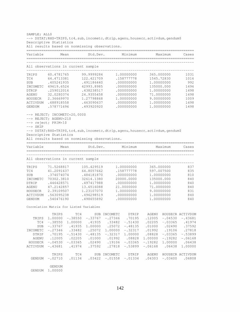
142

SAMPLE; ALL$ --> DSTAT;RHS=TRIPS,tc4,sub,incometc,dtrip,agenu,housecr,activdum,gendum$ Descriptive Statistics All results based on nonmissing observations. =============================================================================== Variable Mean Std.Dev. Minimum Maximum Cases =============================================================================== ------------------------------------------------------------------------------- All observations in current sample ------------------------------------------------------------------------------- TRIPS 60.4781765 99.9999284 1.00000000 365.000000 1031 TC4 64.4713381 122.421709 .158777778 1545.72830 1016 SUB .405241935 .491186440 .000000000 1.00000000 992 INCOMETC 49619.6524 42993.8985 .000000000 135000.000 1496 DTRIP .259012016 .438238517 .000000000 1.00000000 1498 AGENU 32.0280374 24.9355458 .000000000 71.0000000 1498 HOUSECR 2.36669970 1.27798868 1.00000000 9.00000000 1009 ACTIVDUM .688918558 .463090637 .000000000 1.00000000 1498 GENDUM .578771696 .493920920 .000000000 1.00000000 1498 --> REJECT; INCOMETC<20,000$ --> REJECT; AGENU<21$ --> reject; PRIM<1$ --> SKIP --> DSTAT;RHS=TRIPS,tc4,sub,incometc,dtrip,agenu,housecr,activdum,gendum$ Descriptive Statistics All results based on nonmissing observations. =============================================================================== Variable Mean Std.Dev. Minimum Maximum Cases =============================================================================== ------------------------------------------------------------------------------- All observations in current sample ------------------------------------------------------------------------------- TRIPS 71.5268817 105.429519 1.00000000 365.000000 837 TC4 41.2091637 64.8057662 .158777778 597.007500 835 SUB .374074074 .484181870 .000000000 1.00000000 810 INCOMETC 70302.3810 32614.1380 20000.0000 135000.000 840 DTRIP .446428571 .497417988 .000000000 1.00000000 840 AGENU 47.2142857 13.6516088 21.0000000 71.0000000 840 HOUSECR 2.39109507 1.23107070 1.00000000 9.00000000 831 ACTIVDUM .563095238 .496298519 .000000000 1.00000000 840 GENDUM .540476190 .498655892 .000000000 1.00000000 840

Correlation Matrix for Listed Variables TRIPS TC4 SUB INCOMETC DTRIP AGENU HOUSECR ACTIVDUM TRIPS 1.00000 -.38550 -.33767 -.27346 .70195 .12005 -.04530 -.43681 TC4 -.38550 1.00000 .41935 .33482 -.51430 .02205 -.03365 .41974 SUB -.33767 .41935 1.00000 .25072 -.48135 .01000 .02490 .37592 INCOMETC -.27346 .33482 .25072 1.00000 -.32317 .01992 .19106 .27818 DTRIP .70195 -.51430 -.48135 -.32317 1.00000 .08828 -.03365 -.53899 AGENU .12005 .02205 .01000 .01992 .08828 1.00000 -.19282 -.06168 HOUSECR -.04530 -.03365 .02490 .19106 -.03365 -.19282 1.00000 .06438 ACTIVDUM -.43681 .41974 .37592 .27818 -.53899 -.06168 .06438 1.00000 TRIPS TC4 SUB INCOMETC DTRIP AGENU HOUSECR ACTIVDUM GENDUM -.02710 .01134 .03422 -.01558 -.01334 .04303 -.03400 .06808 GENDUM GENDUM 1.00000

143

regress; lhs=trips; rhs=ONE,tc4,sub,incometc,dtrip,agenu,housecr,activdum... ************************************************************************ * NOTE: Deleted 40 observations with missing data. N is now 800 * ************************************************************************ +-----------------------------------------------------------------------+ | Ordinary least squares regression Weighting variable = none | | Dep. var. = TRIPS Mean= 72.69125000 , S.D.= 104.9634345 | | Model size: Observations = 800, Parameters = 9, Deg.Fr.= 791 | | Residuals: Sum of squares= 4371670.399 , Std.Dev.= 74.34221 | | Fit: R-squared= .503380, Adjusted R-squared = .49836 | | Model test: F[ 8, 791] = 100.22, Prob value = .00000 | | Diagnostic: Log-L = -4577.5684, Restricted(b=0) Log-L = -4857.5402 | | LogAmemiyaPrCrt.= 8.629, Akaike Info. Crt.= 11.466 | | Autocorrel: Durbin-Watson Statistic = 1.85060, Rho = .07470 | +-----------------------------------------------------------------------+ +---------+--------------+----------------+--------+---------+----------+ |Variable | Coefficient | Standard Error |b/St.Er.|P[|Z|>z] | Mean of X| +---------+--------------+----------------+--------+---------+----------+ Constant 8.695144665 13.987821 .622 .5342 TC4 -.2997320059E-01 .50677921E-01 -.591 .5542 40.220770 SUB 3.789525075 6.4363914 .589 .5560 .37250000 INCOMETC -.1463725522E-03 .89407944E-04 -1.637 .1016 70353.750 DTRIP 134.9911206 7.1102638 18.985 .0000 .46250000 AGENU .4687839600 .19913078 2.354 .0186 47.300000 HOUSECR -.2198972855E-01 2.2235556 -.010 .9921 2.3962500 ACTIVDUM -15.23478538 6.5052792 -2.342 .0192 .55625000 GENDUM -3.654902617 5.3042437 -.689 .4908 .54500000 (Note: E+nn or E-nn means multiply by 10 to + or -nn power.) --> regress; lhs=log(trips); rhs=ONE,tc4,sub,incometc,dtrip,agenu,housecr,act... ************************************************************************ * NOTE: Deleted 40 observations with missing data. N is now 800 * ************************************************************************ +-----------------------------------------------------------------------+ | Ordinary least squares regression Weighting variable = none | | Dep. var. = LOGTRIPS Mean= 2.678751425 , S.D.= 2.113745632 | | Model size: Observations = 800, Parameters = 9, Deg.Fr.= 791 | | Residuals: Sum of squares= 560.9588960 , Std.Dev.= .84213 | | Fit: R-squared= .842863, Adjusted R-squared = .84127 | | Model test: F[ 8, 791] = 530.35, Prob value = .00000 | | Diagnostic: Log-L = -993.1652, Restricted(b=0) Log-L = -1733.4198 | | LogAmemiyaPrCrt.= -.332, Akaike Info. Crt.= 2.505 | | Autocorrel: Durbin-Watson Statistic = 1.93959, Rho = .03020 | +-----------------------------------------------------------------------+ +---------+--------------+----------------+--------+---------+----------+ |Variable | Coefficient | Standard Error |b/St.Er.|P[|Z|>z] | Mean of X| +---------+--------------+----------------+--------+---------+----------+ Constant 1.631985589 .15844986 10.300 .0000 TC4 -.5226112957E-02 .57406438E-03 -9.104 .0000 40.220770 SUB -.3863307457E-02 .72909524E-01 -.053 .9577 .37250000 INCOMETC -.1847915732E-05 .10127865E-05 -1.825 .0681 70353.750 DTRIP 3.210711728 .80542949E-01 39.863 .0000 .46250000 AGENU .2752924577E-02 .22556941E-02 1.220 .2223 47.300000 HOUSECR -.6440472768E-02 .25187775E-01 -.256 .7982 2.3962500 ACTIVDUM -.3906749785 .73689864E-01 -5.302 .0000 .55625000 GENDUM .1098979535E-01 .60084892E-01 .183 .8549 .54500000 (Note: E+nn or E-nn means multiply by 10 to + or -nn power.)

144

Poisson;Lhs=TRIPS;Rhs=ONE,tc4,sub,incometc,dtrip,agenu,housecr,activdum,g... model=n;Limit=0;Truncation; keep=yfit$ ************************************************************************ * NOTE: Deleted 40 observations with missing data. N is now 800 * ************************************************************************ +---------------------------------------------+ | Poisson Regression | | Maximum Likelihood Estimates | | Model estimated: May 27, 2004 at 07:52:56PM.| | Dependent variable TRIPS | | Weighting variable None | | Number of observations 800 | | Iterations completed 7 | | Log likelihood function -15971.12 | | Restricted log likelihood -53475.36 | | Chi squared 75008.49 | | Degrees of freedom 8 | | Prob[ChiSqd > value] = .0000000 | | LEFT Truncated data, at Y = 0. | | Chi- squared = 29715.80226 RsqP= .7546 | | G - squared = 28333.68526 RsqD= .7257 | | Overdispersion tests: g=mu(i) : 13.266 | | Overdispersion tests: g=mu(i)^2: 19.027 | +---------------------------------------------+ +---------+--------------+----------------+--------+---------+----------+ |Variable | Coefficient | Standard Error |b/St.Er.|P[|Z|>z] | Mean of X| +---------+--------------+----------------+--------+---------+----------+ Constant 2.135878101 .34221746E-01 62.413 .0000 TC4 -.1564737122E-01 .50695844E-03 -30.865 .0000 40.220770 SUB .1281953571 .12608379E-01 10.167 .0000 .37250000 INCOMETC -.1628686523E-05 .14327879E-06 -11.367 .0000 70353.750 DTRIP 2.857196374 .28125051E-01 101.589 .0000 .46250000 AGENU .4860635484E-02 .28348998E-03 17.146 .0000 47.300000 HOUSECR -.8431476066E-02 .32712301E-02 -2.577 .0100 2.3962500 ACTIVDUM -.1413171384 .10207575E-01 -13.844 .0000 .55625000 GENDUM -.2960283116E-01 .83751915E-02 -3.535 .0004 .54500000 (Note: E+nn or E-nn means multiply by 10 to + or -nn power.) Normal exit from iterations. Exit status=0. +---------------------------------------------+ | Negative Binomial Regression | | Maximum Likelihood Estimates | | Model estimated: May 27, 2004 at 07:52:58PM.| | Dependent variable TRIPS | | Weighting variable None | | Number of observations 800 | | Iterations completed 19 | | Log likelihood function -3108.317 | | Restricted log likelihood -15971.12 | | Chi squared 25725.61 | | Degrees of freedom 1 | | Prob[ChiSqd > value] = .0000000 | | LEFT Truncated data, at Y = 0. |

145

+---------+--------------+----------------+--------+---------+----------+ |Variable | Coefficient | Standard Error |b/St.Er.|P[|Z|>z] | Mean of X| +---------+--------------+----------------+--------+---------+----------+ Constant 2.164866409 .15992641 13.537 .0000 TC4 -.1376742919E-01 .64328504E-03 -21.402 .0000 40.220770 SUB .2368818713E-01 .68495354E-01 .346 .7295 .37250000 INCOMETC -.1814165180E-05 .11210026E-05 -1.618 .1056 70353.750 DTRIP 3.010820316 .83480736E-01 36.066 .0000 .46250000 AGENU .2098143747E-02 .23546206E-02 .891 .3729 47.300000 HOUSECR -.2705290695E-01 .27166533E-01 -.996 .3193 2.3962500 ACTIVDUM -.3137841576 .71900663E-01 -4.364 .0000 .55625000 GENDUM .9990263300E-01 .62100762E-01 1.609 .1077 .54500000 Dispersion parameter for count data model Alpha .6449648816 .57790312E-01 11.160 .0000 (Note: E+nn or E-nn means multiply by 10 to + or -nn power.) --> MATRIX; B; VARB; BTC=PART(B,2,2); VBTC=PART(VARB,2,2,2,2) $ --> CREATE; CSBASE= -1/BTC; CSHYR= -Trips/BTC; CSHYRP= -YFIT/BTC; CSBPP=CSBASE/HOUSECR$ --> CALC; LIST; ECS=XBR(CSBASE); ECSYR=XBR(CShYR); ECShYRP = XBR(CShYRP); ECSBPP=XBR(CSBPP); VARCS=VBTC/(BTC^4); CS90L=(-1/BTC) -(1.64*VARCS^.5); CS90U=(-1/BTC)+(1.64*VARCS^.5)$ ECS = .72635201992394390D+02 ECSYR = .51953695016495880D+04 ECSHYRP = .53425454295004390D+04 ECSBPP = .38900199830050930D+02 VARCS = .11518488761957780D+02 CS90L = .67069222530147220D+02 CS90U = .78201181454642320D+02 Calculator: Computed 7 scalar results --> CALC; LIST; AVTC=XBR(tc4); ELAS=BTC*AVTC $ AVTC = .41209163730000320D+02 ELAS = -.56734424355720940D+00 Calculator: Computed 2 scalar results

Appendix D – Significance Test Local- Winter/Summer Trips 11.45 – 12.20 tstat = Sqrt ( 106.17/854 + 92.22/782)

146

t-stat = -1.52, t-crit = -1.96 Fail to reject the hypothesis that there is a significant difference between winter and summer trips made by locals. PPDU-Winter/Summer Expenditures 37.22 - 62.39 t-stat = Sqrt (1763.67/33 + 6844.49/136) t-stat = -2.47, t-crit = -1.96 Accept the hypothesis that there is a significant difference between winter and summer expenditures. PPON-Winter/Summer Expenditures 445.96 - 352.90 t-stat = Sqrt (215935.48/26 + 163141.38/121) t-stat = .947, t-crit = 1.96 No significant difference. NPDU- Winter/Summer Expenditures 24.39 – 61.36 t-stat = Sqrt (552.87/6 + 21261.65/17) t-stat = -1.009, t-crit = -2.069 No significant difference NPON - Winter/Summer Expenditures 27.85 – 22.47 t-stat = Sqrt (2277.02/24 + 668.94/70) t-stat = .526, t-crit = 1.98 No significant difference

147

v