the very basic core of a man's living spirit is his
TRANSCRIPT

The very basic core of a man's living spirit is his passion for adventure. The joy of life comes from our
encounters with new experiences, and hence there is no greater joy than to have an endlessly
changing horizon, for each day to have a new and different sun.
― Christopher McCandless
Promoters Prof. dr. Colin Janssen Environmental Toxicology Unit (GhEnToxLab) Department of Applied Ecology and Environmental Ecology Ghent University Prof. dr. ir. Frederik De Laender Laboratory of Environmental Ecosystem Ecology Research Unit in Environmental and Evolutionary Biology Department of Biology University of Namur Dean Prof dr. ir. Marc van Meirvenne
Rector Prof. dr. Anne De Paepe
Karel VIAENE
Improving ecological realism in the risk assessment of chemicals:
Development of an integrated model
Thesis submitted in fulfilment of the requirements for the degree of Doctor (PhD) in Applied Biological Sciences
Proefschrift voorgedragen tot het bekomen van de graad Doctor in de Bio-ingenieurwetenschappen
Dutch translation of the title:
Verhoging van de ecologische realiteit in de risicoschatting van chemische stoffen: Ontwikkeling van een geïntegreerd model
Refer to this work as:
Viaene K., 2016, Improving ecological realism in the risk assessment of chemicals: development of an integrated model. PhD Thesis, Ghent University, Belgium.
ISBN 978-90-5989-891-2
The author and promoter give the authorisation to consult and to copy parts of this work for personal use only. Any other use is limited by the Law of Copyright. Permission to reproduce any material contained in this work should be obtained from the author.
TABLE OF CONTENTS
CHAPTER 1 GENERAL INTRODUCTION AND OUTLINE p. 1
CHAPTER 2 SPECIES INTERACTIONS AND CHEMICAL STRESS: COMBINED EFFECTS OF INTRASPECIFIC AND INTERSPECIFIC INTERACTIONS AND PYRENE ON DAPHNIA MAGNA POPULATION DYNAMICS
p. 19
CHAPTER 3 DEVELOPMENT OF THE DEBKISS IBM p. 39
CHAPTER 4 APPLICATION OF THE DEBKISS IBM FRAMEWORK TO ASSESS POPULATION-LEVEL EFFECTS OF COMPETITION AND CHEMICAL STRESS
p. 51
CHAPTER 5 DEVELOPMENT OF THE INTEGRATED CHIMERA MODEL p. 67
CHAPTER 6 THE CHIMERA MODEL AS A SCENARIO ANALYSIS TOOL p. 81
CHAPTER 7 GENERAL CONCLUSIONS p. 121
APPENDIX A p. 131
APPENDIX B p. 145
APPENDIX C p. 149
APPENDIX D p. 155
REFERENCES p. 157
SUMMARY p. 169
SAMENVATTING p. 173
DANKWOORD p. 177
CURRICULUM VITAE p. 181
LIST OF ABBREVIATIONS
μg microgram
CR Concentration-response
d Day
DEB Dynamic Energy Budget
DEBkiss Dynamic Energy Budget, Keep It Simple, Stupid
dw Dry weight
EC European Commission
ERA Ecological Risk Assessment
EU European Union
FOCUS FOrum for the Co-ordination of pesticide fate models and their Use
h Hour
HC5 Harmful Concentration for 5% of the species
IBM Individual-based Model
ind individuals
K Phytoplankton carrying capacity
L Litre
mg Milligram
mL Millilitre
mm Millimetre
PEC Predicted Environmental Concentration
PNEC Predicted No Effect Concentration
REACH Registration, Evaluation, Authorisation and Restriction of Chemicals
RQ Risk Quotient
SCHER Scientific Committee on Health and Environmental Risks
SSD Species Sensitivity Distribution
TKTD Toxicokinetic-toxicodynamic
WFD Water Framework Directive
ww Wet weight

1
1 GENERAL INTRODUCTION AND OUTLINE
Chapter 1
2
1.2. Ecological risk assessment
Awareness for the anthropogenic impact on the environment has greatly increased the past decades.
Human activities have been recognized as the major cause of climate change, biodiversity loss and
disruption of nutrient cycles (Hooper et al. 2005; Cardinale et al. 2012). Public reports of massive
animal mortality after e.g. oil spills such as the Deepwater Horizon disaster (Abbriano et al. 2011) are
typically observed following accidental discharges of chemical waste e.g. the 2015 dam burst in a
Brazilian mine (UN Human Rigths 2015). However, pollution also affects ecosystems at smaller spatial
scales and many effects are more subtle and do not necessarily lead to mass mortality of individuals
(Fleeger et al. 2003). In order to prevent such effects, it is important to quantify the risk a chemical poses
to the ecosystem to make informed decisions about its production and use. Most chemicals are potential
hazards for ecosystems i.e. they have inherent properties that can cause damage to the ecosystem (van
Leeuwen and Vermeire 2007). The ecological risk of a chemical refers to the probability that a chemical
will cause damage to the ecosystem, taking into account exposure. Quantification of the risk a chemical
poses for the ecosystem is done by performing an ecological risk assessment (ERA).
In general, the goal of ecological risk assessment of chemicals is to quantify the risk that a concentration
of a given chemical would impair the structure and functioning of natural ecosystems and to derive
maximum environmental concentrations that prevent ecological effects (Preston 2002; De Laender and
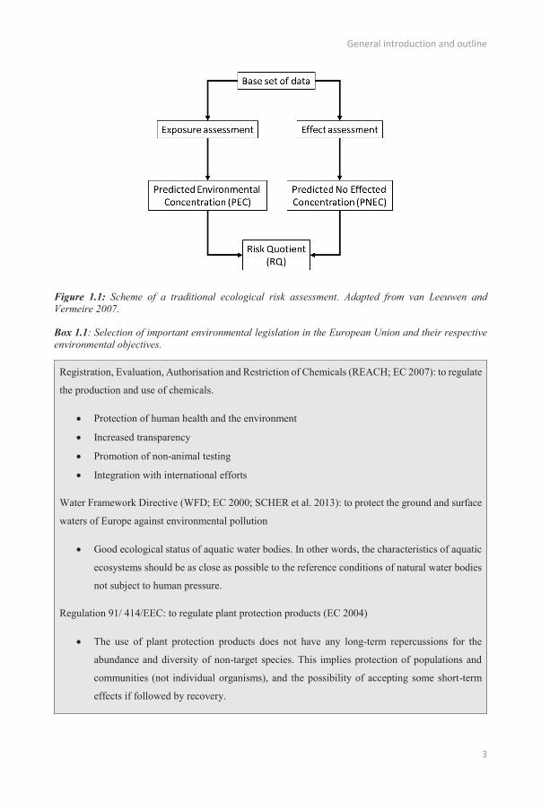
Janssen 2013). Typically, ecological risk assessment is divided in two parts: exposure assessment and
assessment of the potential ecological effects (Figure 1.1; van Leeuwen and Vermeire 2007). Exposure
assessment is used to determine the concentration to which the ecosystem will be exposed. In Europe,
this is typically the Predicted Environmental Concentration (PEC). Chemicals in the environment
undergo different processes such as (bio)degradation, absorption and evaporation (Chapman et al. 1998).
All these processes will determine the final bioavailable concentration i.e. the concentration to which
organisms are actually exposed. Effect assessment is used to determine the Predicted No Effect
Concentration (PNEC), a threshold environmental concentration below which effects to the ecosystem
are not expected to occur. Traditionally, the PEC value is divided by the PNEC to calculate the Risk
Quotient (RQ). RQ values higher than 1 indicate potential risk when the chemical of concern would be
released in the environment without mitigation measures.
General introduction and outline
3
Figure 1.1: Scheme of a traditional ecological risk assessment. Adapted from van Leeuwen and Vermeire 2007.
Box 1.1: Selection of important environmental legislation in the European Union and their respective environmental objectives.
Registration, Evaluation, Authorisation and Restriction of Chemicals (REACH; EC 2007): to regulate
the production and use of chemicals.
Protection of human health and the environment
Increased transparency
Promotion of non-animal testing
Integration with international efforts
Water Framework Directive (WFD; EC 2000; SCHER et al. 2013): to protect the ground and surface
waters of Europe against environmental pollution
Good ecological status of aquatic water bodies. In other words, the characteristics of aquatic
ecosystems should be as close as possible to the reference conditions of natural water bodies
not subject to human pressure.
Regulation 91/ 414/EEC: to regulate plant protection products (EC 2004)
The use of plant protection products does not have any long-term repercussions for the
abundance and diversity of non-target species. This implies protection of populations and
communities (not individual organisms), and the possibility of accepting some short-term
effects if followed by recovery.
Chapter 1
4
Legislation has been developed to prevent environmental risk by performing predictive risk assessments
and specifying formal environmental protection goals. In Europe, several legislations were adopted over
the years (Box 1.1). Biodiversity and ecosystem functions are usually specified as protection goals
(Hommen et al. 2010). For example, the European Commission has made a commitment towards
“halting the loss of biodiversity and the degradation of ecosystem services in the EU by 2020” (EU,
2010) and, according to the Water Framework Directive (WFD), all European surface and groundwater
bodies should have a good ecological status by 2015 (EU, 2000). The focus on biodiversity in legislation
is understandable as biodiversity is generally considered an useful descriptor of ecosystem structure and
its role in ecosystem productivity and stability is generally accepted in the ecological literature (Hooper
et al. 2005, 2012; Cardinale et al. 2012).
1.3. Current ERA methods and their limitations
The number of registered chemicals is approximately 100,000 and still increasing (Clements and Rohr
2009). To cope with this high number of chemicals, ERA is typically conducted using a tiered approach
(Figure 1.2) i.e. chemicals that pose a higher risk at lower tiers are subjected to more extensive and
complex risk assessment methods at higher tiers (Brock et al. 2006; SCHER et al. 2013). The lowest tier
is primarily used for screening chemicals i.e. identification of chemicals that could pose a risk. This
lowest tier is very similar in all EU directives and is based on the risk quotient i.e. the ratio of the PEC
and the concentration at which effects are expected (Hommen et al. 2010). In all directives except for
the plant protection directive, the Predicted No Effect Concentration (PNEC) is used as the reference
concentration for effects. The PNEC is calculated by dividing the endpoint of the most sensitive test
species by an appropriate assessment factor. Assessment factors, also sometimes called safety factors,
are used to account for uncertainty concerning the accuracy of the selected endpoint such as intra- and
interspecies differences in sensitivity, differences between acute and chronic tests and the lab-to-field
extrapolation (Chapman et al. 1998). If the risk quotient is larger than 1, the chemical has a potential
risk to the environment and needs to either undergo higher tier risk assessment to further assess the risk
or be risk managed.
The use of the risk quotient, and especially assessment factors, has been heavily criticized in ERA.
Assessment factors are a conservative method to deal with the uncertainty related to the extrapolation
to real situations but are based on policy and not on science (Chapman et al. 1998; Forbes et al. 2008).
Indeed, this approach relies too much on expert judgement to relate risk ratios to environmental
protection goals (Forbes et al. 2009a). This often leads to an overestimation of the risk and consequently,
unrealistically low “safe” concentrations (Chapman et al. 1998). Also, this approach only uses the most
sensitive endpoint of the available toxicity tests (Forbes et al. 2008). Unless additional toxicity tests
reduce the assessment factor e.g. a chronic test versus an acute test, they are only used to calculate a

General introduction and outline
5
new PNEC when the measured endpoint is even more sensitive than the previous one. More information
on the potential toxicity of a chemical does thus not necessarily lead to more accurate risk assessments
with this approach.
Figure 1.2: The tiered approach to the risk assessment of chemicals. Chemicals that pose a higher risk may be subject to more extensive assessment methods.
Higher tier risk assessment methods include the use of extrapolation models and multi-species test
systems. The species sensitivity distribution (SSD) is the most used extrapolation model and fits a
probability distribution to a set of toxicity thresholds derived in single species toxicity tests (Forbes and
Calow 2002; Posthuma et al. 2002). The probability distribution is used to determine a concentration at
which a certain percentage of the species is not affected. Typically, the concentration at which 95% of
the species are protected is used as the PNEC value. A major advantage of this approach compared to
the risk quotient technique is that it incorporates all information available from different species. The
SSD approach has been compared with model ecosystem data and field data for many chemicals e.g. for
endosulfan (Hose and Van den Brink 2004) and fluazinam (van Wijngaarden et al. 2005). Indeed, most
SSD-derived treshold concentrations were protective for ecosystem structure and functioning (Versteeg
et al. 1999). However, the properties and underlying assumptions of SSDs have been discussed in depth
over the years and questions, mainly related to their underlying assumptions, have been raised about
their use for ecological risk assessment (Forbes and Calow 2002).
One of the main issues is that the species included in the SSD are considered as components of a realistic
community while this is rarely the case (Forbes and Calow 2002). Generally, any organism for which
sensitivity data are available is included and this species is assumed to be equally important for structure
and functioning of the ecosystem. This ignores the possible presence of keystone species which have a
larger than average contribution to ecosystem structure and functioning. Also, SSDs assume that
interactions between individuals and species will not influence the sensitivity of the community (De
Laender et al. 2008c; Schmitt-Jansen et al. 2008). However, there are many examples of how ecological
interactions can influence the outcome of chemical exposure and this assumption is thus unrealistic. For
example, one modelling study compared a SSD approach that neglected ecological interactions with one
that accounted for ecological interactions (De Laender et al. 2008c). The latter study showed that for
approximately 25% of the toxicants, the SSD approach that took ecological interactions into account

Chapter 1
6
was more strict than the SSD approach that neglected ecological interactions. Therefore, it is impossible
to determine if derived safe concentrations with a SSD are protective for real ecological communities.
Several statistical considerations need to be accounted for when applying SSDs. To calculate accurate
percentiles, a sufficient number of species needs to be included and the appropriate distribution should
be used. The amount of species needed differs between cases but has been estimated to range between
15 and 55 species (Newman et al. 2000). This is higher than what is required for most regulatory
purposes and for most chemicals this amount of data is not available. Also, the identity of the species
included in the SSD will influence the derived safe concentrations (Forbes et al. 2001; De Laender et al.
2013). Inclusion of a large number of species sensitive to a certain chemical e.g. primary producer for a
photo-synthesis inhibiting herbicide, will lead to lower safe concentrations than a set of species where
primary producers are under-represented (Van den Brink et al. 2006). To fit the SSD to the data, the log-
normal distribution is often chosen but this distribution is often not applicable to the data (Newman et
al. 2000). These statistical considerations are often neglected which leads to inaccurate predictions and
a high uncertainty on the derived percentiles and thus ‘safe’ concentrations (Forbes and Calow 2002).
Finally, questions can be raised about how a SSD is used and interpreted. Often the HC5 i.e. the
concentration at which 5% of all species are affected, is calculated and used as a safe environmental
concentration. This assumes that 5% of the species is an appropriate protection level i.e. that the loss of
5% of the species does not affect the ecosystem structure and functioning (functional redundancy) and
that biodiversity, as a measure of ecosystem structure, is a more sensitive ecosystem endpoint than
ecosystem functions (Newman et al. 2000; Forbes and Calow 2002; De Laender et al. 2008a). This
appears to be true for herbicides, insecticides and fungicides: comparison between SSD-derived HC5
values and no-effect concentrations in model communities showed that HC5 values were, in general,
protective for at least short-term exposure (Van den Brink et al. 2006; Maltby et al. 2009). For
insecticides, the SSD-approach was protective in 25 of the 27 cases when compared with experiments
with model communities (van Wijngaarden et al. 2015). Further evaluation is however required for
chemicals that have chronic toxicity or modes of action that have been rarely tested e.g. neonicotinoids.
Experiments with model communities, both small scale (microcosms) and large scale (mesocosms), are
currently considered the most ecologically relevant effect assessment techniques because they expose
realistic aquatic communities over a longer period of time to the chemical (Schmitt-Jansen et al. 2008).
This approach can account for ecological interactions and indirect effects i.e. effects on tolerant species
through interactions with sensitive species (Fleeger et al. 2003; De Laender et al. 2011). Population and
ecosystem recovery can also be assessed with this method. However, micro- and mesocosms also have
several disadvantages. The amount of time and resources required to perform such experiments is a
major drawback (De Laender et al. 2013). Also, interpretation of the results is non-trivial, although
methods like the principal response curve technique have been developed to deal with this (Van den
Brink and Ter Braak 1998). Other disadvantages include problems with scaling effects, the protection

General introduction and outline
7
of rare species, sensitivity to starting conditions and the inability to replicate every natural system
(Forbes et al. 2008; Schmitt-Jansen et al. 2008). Effects occurring in the model communities do not
necessarily correspond with effects at more realistic spatial scales, referred to as scaling effects (Forbes
et al. 2008). For example, in realistic landscapes, migration of individuals can alter the observed effects.
Moreover, model communities might miss effects on rare species not present in the sampled community.
Species can also be sensitive to the starting conditions of the model community experiment, reducing
the relevance of the experiments (Hjorth et al. 2007). Lastly, it is impossible to perform such
experiments for each natural system. Comparison between different communities exposed to the same
chemical has shown that, although the sensitive species are affected at similar concentrations, indirect
effects and recovery can indeed be very different (Daam and Van den Brink 2010).
In general, all current ERA methods fail to provide an accurate and certain answer to the central question
in ecotoxicology: what are the large-scale effects of chemical stress in real-world systems (Beketov and
Liess 2012). As a result, decisions in risk assessment are accompanied with large uncertainty and the
prescribed protective concentrations are possibly either under- or overprotective. The major problem is
how to extrapolate from these, at best, simple community tests performed in a controlled environment
to the protection goals set by the authorities (De Laender et al. 2008a; Forbes et al. 2008). The
relationship between typical ecotoxicological endpoints such as growth, survival and fecundity and
population or ecosystem dynamics is complex, non-linear and thus difficult to predict using simple
techniques (Forbes et al. 2008). Therefore, ecological risk cannot be adequately assessed using
procedures that disregard most of the inherent environmental and ecological complexity (De Laender et
al. 2014a). However, current ERA procedures fail to consider newly developed methods such as
ecological models that were specifically developed to reduce the uncertainty in ERA. Also, it is unclear
that current approaches are able to accurately predict future risks, especially considering that the number
of environmental stressors are increasing (Grimm and Martin 2013). Multiple stressors can refer to a
combination of different chemicals but also to the combination of chemicals and other abiotic stressors
such as temperature (De Laender and Janssen 2013). How these multiple stressors interact is difficult to
predict (Gabsi et al. 2014b) but it is clear that the presence of multiple stressors may have potentially
large implications for ERA.
1.4. Integration of ecology into the risk assessment procedure
In order to more accurately predict the effects of chemicals on communities and ecosystems, more
ecology needs to be integrated in ERA approaches (Chapman 2002; Clements and Rohr 2009; Grimm
et al. 2009). The call for integration of ecological processes was already brought up as early as the 1980s
– “putting the eco in ecotoxicology” (Cairns 1988) – and 1990s (Baird et al. 1996). Recent notable
efforts call for the integration of macro-ecology in ecotoxicology (Beketov and Liess 2012) and for the
Chapter 1
8
application of community ecology to ecotoxicological theory (Schmitt-Jansen et al. 2008). Scientific
efforts have been done to address these concerns e.g. the use of ecological models (Galic et al. 2010).
However, integration of more ecology at the regulatory level has thus far been limited to the use of
micro- and mesocosm experiments as highest tier ERA tools. Criticism of the current ERA procedures
was summarized in an opinion report of different Scientific Committees of the European Union (SCHER
et al. 2013). The report recognizes that current ERA procedures lack ecological realism which leads to
high uncertainty associated with the predictions made.
With the current advances in ecological modelling and informatics, it should be feasible to use more
complex and computationally intensive techniques that are better at integrating ecological principles.
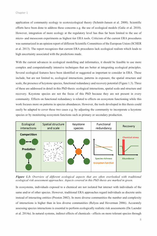
Several ecological features have been identified or suggested as important to consider in ERA. These
include, but are not limited to, ecological interactions, patterns in exposure, the spatial structure and
scale, the presence of keystone species, functional redundancy and recovery potential (Figure 1.3). Three
of these are addressed in detail in this PhD thesis: ecological interactions, spatial scale and structure and
recovery. Keystone species are not the focus of this PhD because they are not present in every
community. Effects on functional redundancy is related to effects on ecosystem functioning while this
work focuses more on patterns in species abundances. However, the tools developed in this thesis could
easily be adapted to cover these two cases e.g. by adjusting the community to incorporate a keystone
species or by monitoring ecosystem functions such as primary or secondary production.
Figure 1.3: Overview of different ecological aspects that are often overlooked with traditional ecological risk assessment approaches. Aspects covered in this PhD thesis are marked in green.
In ecosystems, individuals exposed to a chemical are not isolated but interact with individuals of the
same and/or of other species. However, traditional ERA approaches regard individuals as discrete units
instead of interacting entities (Preston 2002). In more diverse communities the number and complexity
of interactions is higher than in less diverse communities (Relyea and Hoverman 2006). Accurately
assessing species interactions is essential to perform ecologically realistic risk assessments (De Laender
et al. 2014a). In natural systems, indirect effects of chemicals - effects on more tolerant species through

General introduction and outline
9
interactions with sensitive species - are common (Rohr et al. 2006; Clements and Rohr 2009). Because
they involve multiple species, indirect effects are also intrinsically more complex and more difficult to
predict (Rohr et al. 2006). Competition and predation are regarded as the most important ecological
interactions when considering indirect effects of chemicals (Preston 2002).
Competition can refer to competition for the same food source but also to competition for space, light
or other limiting resources. Competition can occur between individuals of different species (interspecific
competition) but also within one population of the same species (intraspecific competition). Generally,
when chemical stress leads to decreased population densities, the surviving individuals in the population
experience less intraspecific competition (Foit et al. 2012). This decreased intraspecific competition
reduces the effect of chemical stress on population densities (Liess 2002; Foit et al. 2012; Del Arco et
al. 2015) and allows more rapid recovery of population density or size structure after exposure (Foit et
al. 2012; Knillmann et al. 2012b). For competition between tolerant and sensitive species, tolerant
species are expected to be, at least partly, relieved from competition (Foit et al. 2012). Consequently,
the tolerant species perform better after exposure to stress. This was experimentally shown for Daphnia
magna and Culex sp. larvae exposed to fenvalerate (Foit et al. 2012) and for Daphnia spp. in microcosms
exposed to esfenvalerate (Knillmann et al. 2012b). Other examples include modelling studies where
competition prolonged the effects of the chemical (Kattwinkel and Liess 2013) or increased the
vulnerability of the population to chemical stress (Gabsi et al. 2014b). In reality, species can interact in
other ways than only via competition. For example, in an experiment with Asellus aquaticus and
Gammarus pulex, competition positively influenced G. pulex survival during exposure to carbendazim
(Del Arco et al. 2015). This was attributed to predatory compensatory mechanisms by G. pulex under
food-limited conditions, showing that reality can be much more complex and unpredictable than
standard experiments would suggest.
For predation, chemical stress can either affect the prey, the predator, or both. Similarly to interspecific
competition, effects on the predator may relieve the prey species from predation, allowing it to increase
in abundance (Fleeger et al. 2003). For example, phytoplankton species increased in abundance after
elimination of the grazers due to carbendazim toxicity (Van den Brink et al. 2000). A common
observation when prey are more sensitive than predators is that prey exposed to a toxicant are more
vulnerable to predation (Fleeger et al. 2003; Beketov and Liess 2006). For example, Artemia sp.
populations went extinct after combined exposure to chemical stress and simulated predation (Beketov
and Liess 2006). In this case, the predation pressure prevented density-dependent compensation for the
chemical effect i.e. increased reproduction at low densities was not possible. Chironomus larvae were
less active after cadmium exposure (Rooks et al. 2009). This increased their susceptibility to active
predators but interestingly, the predation rate by ambush predators was not affected. Predator species
can also be affected by chemical stress through their prey e.g. ciliates starved when their food source
was eliminated by prometryn (Liebig et al. 2008). However, predation does not always lead to higher
Chapter 1
10
effects of a chemical. Presence of predator kairomones resulted in Daphnia magna producing larger
offspring that were more resistant to chemicals, thus reducing the effect of carbaryl exposure (Coors and
Meester 2008; Gergs et al. 2013). How chemical stress interacts with competition and predation is
clearly chemical and species specific. To predict how these interactions influence the effect of
chemicals, a better understanding of the underlying processes is needed.
Differences in application time, emission rates and location can result in significant differences in timing
and levels of exposure, ultimately leading to different effects on local populations (Galic et al. 2012).
Depending on the chemical identity, exposure patterns can differ greatly (De Laender et al. 2014a).
Chemicals differ in their application time, partition to different compartments in the environment and
differ in their persistence in the environment. These realistic exposure patterns can differ greatly from
typical lab tests with short, constant exposure. Another important aspect is the timing of exposure in the
life cycle of the exposed populations. Early life stages, especially embryonic stages, are often more
sensitive to chemicals. Exposure during periods of reproduction can thus lead to larger population effects
than exposure during periods of no reproduction, especially for species with long life cycles (Bridges
2000; Galic et al. 2012). The landscape structure and the presence of unexposed populations is another
factor determining the outcome of chemical exposure and is especially important for the recovery of the
affected populations. For example, isolated communities recovered more slowly from the application of
endosulfan than less isolated communities (Trekels et al. 2011). Similarly, the presence of
uncontaminated patches decreased the recovery time of mesocosm communities after lufenuron
exposure (Brock et al. 2009).
“Keystone species” are species that are essential for certain ecosystem functions or that enable other
species to survive in the ecosystem (Chapman 2002). Keystone species often indicate the presence of
an ecological threshold and the loss of these keystone species often results in abrupt, non-linear changes
in ecosystem structure and functioning that are difficult to recover from (Clements and Rohr 2009). For
example, the burrowing ghost shrimp Neotrypaea californiensis is an important facilitator for many
other species of the soft sediment benthos. Direct effects of carbaryl on this shrimp species also
indirectly affected the associated benthos species (Dumbauld et al. 2001). Therefore, it is important to
identify the presence and identity of keystone species in ecosystems. Closely related to this is the concept
of functional redundancy. Functional redundancy occurs when the loss of some species does not result
in the loss of ecosystem functioning because more tolerant species compensate for the affected species
(Chapman 2002). Not all species are thus always equally important for the ecosystem structure and
functioning and ecological risk assessments should take this into account.
Another often neglected characteristic of natural populations is their potential to recover after a
disturbance event. In natural ecosystems, populations are regularly disturbed by environmental factors.
If we consider the long-term effects of chemicals, the recovery potential of a population or ecosystem
General introduction and outline
11
is thus an important factor (Relyea and Hoverman 2006; Clements and Rohr 2009). The recovery
potential differs between species and systems e.g. short lived species will typically recover quicker from
chemical stress than species with a longer life cycle, and is influenced by other environmental factors
e.g. indirect effects (De Lange et al. 2010; Knillmann et al. 2012b). Ideally, ecological risk assessments
should take the recovery potential of a system into account and be more stringent when the recovery
potential is low.
1.5. Modelling as a risk assessment tool
A main challenge in the field of ecotoxicology is to develop tools that can take into account the
ecological complexity displayed in real ecosystems (Figure 1.3) so that site-specific effects can be
assessed. Ecological modelling was proposed as one of the best options to improve effect assessment,
specifically to account for ecological interactions and spatial and temporal variability in exposure
(SCHER et al. 2013). However, the use of models is far less accepted in effect assessment than in
exposure assessment. In particular, the development of FOCUS (FOrum for the Co-ordination of
pesticide fate models and their Use; FOCUS 2001) models and scenarios provided a standardized way
to develop and use environmental fate models (Grimm and Martin 2013; SCHER et al. 2013). The
inherent complexity of ecosystems, the apparent lack of universal ecological laws and the lack of clear
protection goals have hindered the acceptance of models as tools for effect assessment of chemicals
(Van Straalen 2003; Van den Brink et al. 2006). In legislation, ecological models are thus mostly ignored
as possible ERA tools. Only the guidance document relating to aquatic toxicology under Directive
91/414/ EEC (SANCO 2002) lists ecological models as possible tools in higher tiered risk assessments
for extrapolation from microcosm or mesocosm studies to the field (Hommen et al. 2010). It is clear that
more ecological knowledge and more complex decision making is required to apply ecological models
as tools for effect assessment (Dohmen et al. 2015). Indeed, modelling could be an ecology based
alternative to the standard ERA approaches and can actually be used to assess the effects of chemicals
on the actual protection goals i.e. biodiversity and ecosystem functioning (De Laender et al. 2008b;
Forbes et al. 2009a). Potential applications of models in ERA include (i) evaluating the relevance of
effects on individuals for population dynamics, (ii) extrapolation to untested exposure patterns, (iii)
extrapolation of recovery processes from lab to field, (iv) assessment of indirect effects and (v)
evaluation of bioaccumulation and biomagnification of chemicals (Hommen et al. 2010). Several
initiatives have been taken during the past decade to explore and promote the use of ecological models
in risk assessment e.g. the CREAM (Grimm et al. 2009) and ChimERA (De Laender et al. 2014a)
projects, as well as through the establishment of the MemoRisk SETAC advisory group (Preuss et al.
2009b) and the organization of several workshops e.g. LEMTOX (Forbes et al. 2009b) and
MODELLINK (Hommen et al. 2016).
Chapter 1
12
Using models to assess the effects of chemicals on populations, communities or ecosystems has several
advantages. Most importantly, models can help clarify how chemicals affect higher levels of biological
organization, why certain effects are happening and what the most important drivers are (Grimm et al.
2009). Ecological models have successfully been used to comprehend and predict the effects of
chemicals on populations (Galic et al. 2010; Preuss et al. 2010; Dohmen et al. 2015), communities (De
Laender et al. 2014b), and ecosystems (De Laender et al. 2015). With advances in computational power
and efficiency, the explicit consideration of time and space in models is becoming more feasible (Galic
et al. 2010). This allows the modelling of populations in heterogeneous landscapes, where the exposure
can be drastically different between different locations and different times of the year. Modelled Asellus
aquaticus populations were predicted to recover faster when connectivity in the habitat was higher
(Galic et al. 2012). Exposure during periods of reproduction resulted in slower recovery, indicating the
importance of the exposure profile. Models are also ideally suited to study how effects on individuals
translate to effects on population and ecosystem dynamics (Bradbury et al. 2004; Forbes and Calow
2012). For example, evaluation of different physiological modes of actions in Daphnia magna
populations showed that direct effects on survival and reproduction had a much larger impact on
population densities than effects on growth or feeding rate (Gabsi et al. 2014a). Modelling can thus help
reduce the uncertainty associated with the extrapolation from ecotoxicological observations to
ecological effects (Forbes et al. 2008).
Modelling approaches can also be informative for the lower tiers of risk assessment. Experiments in
silico can help to design toxicity tests, interpret individual responses to chemical stress and identify
deficits in current datasets, allowing for more focused experimental work (Galic et al. 2010; Jager et al.
2014). Moreover, the large amount of historical ecotoxicology data can be used for modelling purposes
and models can reduce the need for additional ecotoxicological tests, reducing the amount of test animals
needed.
1.6. Individual based modelling
Individual based models (IBMs) seem particularly suited for use in ERA. IBMs consider processes
occurring at the individual level such as feeding, growth and reproduction (Martin et al. 2013b; Gabsi
et al. 2014b). Population properties are not modelled directly but emerge from the individuals in the
population. Since most ecotoxicological tests focus on the individual level, IBMs are ideal tools to
translate these test results to the population level. Incorporating chemical effects on individuals in IBMs
allows exploration of the effects of chemicals at the population level. In recent years, IBMs have been
used to predict the population dynamics of a number of typical test species used in ecotoxicology e.g.
Daphnia magna (Preuss et al. 2010; Martin et al. 2013a) and Asellus aquaticus (Galic et al. 2012).
Similarly, the effects of a hypothetical insecticide on three populations of arthropods were modelled

General introduction and outline
13
using individual based models (Dohmen et al. 2015). These IBM applications neglected possible
interactions with other species and focused solely on a single species. However, the absence of
interactions between species is one of the main criticisms on current ERA methods (Rohr et al. 2006;
Clements and Rohr 2009). Considering that ecological models have been suggested as tools to
extrapolate individual-level effects observed in experiments to population, food web and ecosystem
level effects (Grimm et al. 2009; De Laender et al. 2014a), it is important to develop ecological models
that do incorporate interactions between species. One recent modelling effort showed that adding
interspecific competition to individual-based models increased recovery times following chemical stress
up to three times (Kattwinkel and Liess 2013). IBMs have however not been applied yet for more
complex systems e.g. food webs, where more species and more interactions between these species need
to be considered.
1.7. Current limitations to using modelling in risk assessment
Modelling could be useful to overcome many of the shortcomings of current ERA procedures. However,
modelling needs to improve in certain key areas before it will be fully accepted as an ERA tool. These
improvements are two-fold: (1) improvements of the science underlying the models and (2)
improvements of the regulatory use of models (Grimm and Martin 2013). To improve the science behind
the models, validation is of key importance i.e. how can we know that developed models capture reality,
that the science is sound (Forbes et al. 2008; Grimm and Martin 2013)? Validation is, however, a very
broad term and unclear terminology is often an obstacle to understand what validation entails (Augusiak
et al. 2014). A better defined validation process such as the evaludation process defined by Augusiak et
al. 2014, will increase the acceptance of models and increase the understanding of the science behind it.
Validation is closely linked to the emergence of patterns from data (Grimm and Martin 2013).
Observations are considered patterns if they are unlikely to result from random processes and thus
contain information about the underlying organization. By comparing model output with these patterns,
we can validate the model i.e. assess if the model accurately captures the underlying processes and is
thus a realistic, scientifically sound representation of the world. A related scientific question is how
general does a model need to be, how much complexity does it need, to accurately answer the questions
posed (Forbes et al. 2008). In general, more complex models can predict the outcome more accurately
but are harder to validate. The selection of the correct level of complexity for the focus situation is thus
essential.
To improve the regulatory use of models, risk assessors need to be convinced of their accuracy and
potential (Forbes et al. 2009b; Grimm and Martin 2013). Risk assessors are usually not trained in
modelling and cannot be expected to accurately assess the appropriateness and validity of a model. For
exposure assessment, this problem was solved by developing the FOCUS framework (FOCUS 2001).
Chapter 1
14
This provided risk assessors with a standard way to evaluate exposure models. A similar standardization
is needed for ecological models. Some efforts have been made to promote the use of ecological models
for ERA e.g. The EU-funded CREAM project (Chemical Risk Effects Assessment models; Grimm et
al. 2009; Grimm and Thorbek 2014). Similarly, good modelling practices such as the ODD (overview,
design concepts and details) protocol and TRACE (transparent and comprehensive ecological
modelling) have been developed (Grimm et al. 2006; Schmolke et al. 2010).
1.8. Problem formulation and objectives of this PhD thesis
It is clear that ERA needs state-of-the-art tools to achieve its goal: accurately assessing the risk a
chemical poses to the environment, taking into account essential ecological characteristics of real
systems. One key characteristic that needs to be accounted for are interactions between individuals, both
within one species and between different species. Individual based models (IBMs) are one of the most
promising tools for ERA but their applicability to food webs is unclear. Also, realistic exposure
scenarios, with spatial and temporal variability in exposure, need to be considered. Therefore, the
objectives of this PhD thesis are:
understand how species interactions (competition and predation) interfere with chemical stress;
develop and apply IBMs for two species competing for the same food source;
develop an individual-based food-web model;
develop and apply an integrated ecological risk assessment model (ChimERA) to different
environmental scenarios;
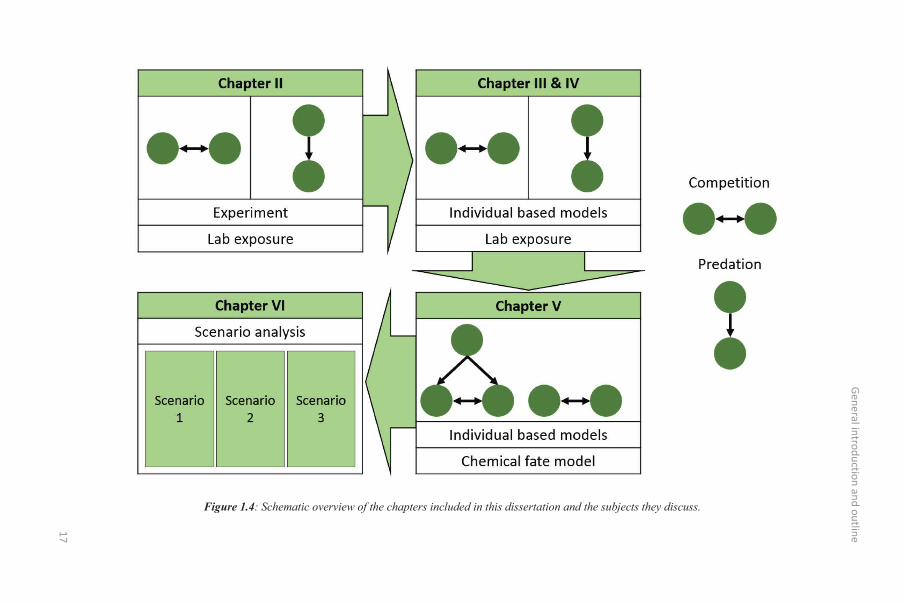
This research is presented in five main chapters (Figure 1.4), increasing the complexity from simple
food webs in the laboratory to more complex food webs in an integrated exposure and effect model. The
main conclusions were summarized in a final chapter.
General introduction and outline
15
1.9. Thesis outline
1.9.1. Species interactions and chemical stress
Interactions between individuals of the same species and of different species will alter how these
individuals respond to chemical stress. To understand how intra- and interspecific competition and
predation can alter the effect of chemical stress, experiments were performed with simple food webs
(Chapter 2). Communities of the water flea Daphnia magna, the rotifer Brachionus calyciflorus and
the phantom midge Chaoborus obscuripes larvae were exposed to pyrene. Effects of pyrene were
expected to be higher in D. magna populations exposed to strong competition or predation. The tolerant
competitor B. calyciflorus was expected to increase in abundance after pyrene exposure. An indirect
negative effect on the predator C. obscuripes was expected through direct pyrene effects on its prey D.
magna.
1.9.2. Modelling competing species under chemical stress
Models can help to understand and predict the effects of chemicals on populations and food webs. IBMs
in particular are useful because effects of chemicals can be included at the level of the individual, the
focal level of standard ecotoxicity tests. To make the IBMs as widely applicable as possible, they should
be based on a generic theory. In Chapter 3, I describe the development of the DEBkiss IBM: an
individual based model based on the DEBkiss theory. Chemical effects were included in the model by
considering effects on survival using either concentration-response curves or toxicokinetic-
toxicodynamics models.
The validity of the DEBkiss IBM framework was tested in Chapter 4 by applying IBMs to the
experiments with D. magna and B. calyciflorus described in Chapter 2. More specifically, I evaluated
whether the DEBkiss IBM framework could simulate the population densities of these two grazers when
exposed to pyrene, interspecific competition and both pyrene exposure and interspecific competition.
This was done by comparing the model simulations with the patterns observed in the experiment.
1.9.3. Food web model development and integration with a fate model: the ChimERA
model
Realistic ecosystems are not limited to two species but consist of many interacting species. In Chapter
5, predation was therefore added to the competition implementation presented in Chapters 3 and 4 and
used to develop an individual-based food web model. Although traditionally separated, exposure and
effect assessment are both integral parts of ecological risk assessment. Chapter 5 is therefore concluded
Chapter 1
16
with the integration of a fate model with the food web model, forming the ChimERA model: a spatially-
explicit model simulating both the fate of a chemical and the effects on the food web.
1.9.4. Scenario analysis with the ChimERA model
A key feature of the integrated ChimERA model is that the effects of different environmental parameters
on the food web dynamics can be evaluated, opening a whole new, prospective approach to ERA. In
Chapter 6, the influence of trophic state, temperature, hydrodynamics and chemical exposure pattern
on the resulting chemical effects were evaluated. Effects of these environmental variables on the
environmental fate of the chemical and on the food web dynamics was assessed.
1.9.5. Conclusion and future directions
In the final Chapter 7, the findings of this dissertation are reviewed and summarized in a set of
conclusions. Suggestions and possible directions for future research are provided.
General introduction and outline
17
Figure 1.4: Schematic overview of the chapters included in this dissertation and the subjects they discuss.
Chapter 11 Chapter 111 & IV
...... • ..... Competition
Experiment lndividual based models
Lab exposure Lab exposure
Predation
ChapterVI ChapterV
Scenario analysis
Sce~ario 11 Sce;ario 11 Sce;ario
Chemica! fate model


19
2 SPECIES INTERACTIONS AND CHEMICAL STRESS:
COMBINED EFFECTS OF INTRASPECIFIC AND
INTERSPECIFIC INTERACTIONS AND PYRENE ON
DAPHNIA MAGNA POPULATION DYNAMICS
Redrafted from:
Viaene KPJ, De Laender F, Rico A, Van den Brink PJ, Di Guardo A, Morselli M, et al. Species
interactions and chemical stress: Combined effects of intraspecific and interspecific interactions and
pyrene on Daphnia magna population dynamics. Environ Toxicol Chem. 2015;34(8):1751–9.
Chapter 2
20
Abstract
Species interactions are often suggested as an important factor when assessing the effects of chemicals
on higher levels of biological organization. Nevertheless, the contribution of intra- and interspecific
interactions to chemical effects on populations is often overlooked. In the current chapter, Daphnia
magna populations were initiated with different levels of intraspecific competition, interspecific
competition and predation and exposed to pyrene pulses. Generalized linear models were used to test
which of these factors significantly explained population size and structure at different time points.
Pyrene had a negative effect on total population densities, with effects being more pronounced on
smaller D. magna individuals. Among all species interactions tested, predation had the largest negative
effect on population densities. Predation and high initial intraspecific competition were shown to
interact antagonistically with pyrene exposure. This was attributed to differences in population
structure prior to pyrene exposure and pyrene-induced reductions in predation pressure by Chaoborus
sp. larvae. The results presented in this chapter provide empirical evidence that species interactions
within and between populations can alter the response of aquatic populations to chemical exposure. It
is concluded that such interactions are important factors to be considered in ecological risk
assessments.

21
2.1. Introduction
Current procedures for the ecological risk assessment (ERA) of chemicals are generally based on the
extrapolation of individual-level responses to the whole ecosystem and often fail to integrate a sufficient
level of ecological realism (De Laender et al. 2008b; SCHER (Scientific Committee on Health and
Environmental Risks) et al. 2013). In ecosystems, individuals exposed to a chemical are rarely isolated
but interact with individuals of the same and/or of another species. Despite being one of the key
characteristics of ecosystems, interactions within and between species are rarely included in current
prospective ERAs, especially for non-pesticidal chemicals (De Laender et al. 2008c). However, species
interactions can alter the direct effects of a chemical on a sensitive species e.g. increased mortality after
pesticide addition because of decreased predator avoidance behavior (Hanazato 2001). Alternatively, by
interacting with sensitive species, tolerant species can also be affected leading to indirect effects of
chemical stress e.g. starvation of the consumer species when the prey species is affected (Rohr and
Crumrine 2005; De Hoop et al. 2013) or reduced competition with the affected species (Rohr and
Crumrine 2005). The indirect effects of a chemical are often overlooked but can be as large or even
larger than the direct effects of the chemical (Fleeger et al. 2003). Interactions with other species can
either increase or decrease the susceptibility of populations and communities to a chemical (Preston
2002; Fleeger et al. 2003). For example, the no observed effect concentration (NOEC) of prometryn for
ciliates was more than two orders of magnitude lower in microcosms compared with a single-species
toxicity test because of the sensitivity of their food source to prometryn (Liebig et al. 2008). Also,
elimination of grazers by the fungicide carbendazim allowed certain phytoplankton species to increase
in abundance (Van den Brink et al. 2000) and exposure to insecticides resulted in the development of
anti-predator structures in daphnids, potentially reducing the effect of predation (Hanazato 2001).
Accurately assessing species interactions is thus essential to perform ecologically realistic chemical risk
assessments (De Laender et al. 2014a).
Competition and predation are regarded as the most important species interactions when considering
indirect effects of chemicals (Preston 2002). Competition can occur between individuals of different
species (interspecific competition) but also within one population of the same species (intraspecific
competition). Although several studies exist on the combined effects of interspecific competition and
chemicals (Foit et al. 2012; Knillmann et al. 2012b), studies on how intraspecific competition affects
the response of populations to chemical exposure are rather underrepresented in the ecotoxicological
literature.
The objective of the current chapter was to investigate how initial differences in species interactions
influence the response of aquatic invertebrate populations to chemical stress. To this end, Daphnia
magna populations were initiated with different levels of intraspecific and interspecific competition and
Chapter 2
22
predation with pyrene as a chemical stressor. Population size and structure of D. magna were evaluated
using generalized linear models. Higher effects of pyrene were expected in populations that are
experiencing increased competition or predation pressure compared to a control population.
2.2. Materials and Methods
2.2.1. Experimental design
D. magna populations were exposed to six levels of species interactions (i.e. species interaction control,
low and high intraspecific competition, low and high interspecific competition, and predation) and to
five different pyrene exposure profiles (i.e. control, solvent control, and low, medium and high exposure;
see Table 2.1). The experiment was performed in triplicate (n = 3). Two additional replicates were added
for the species interaction control treatment without pyrene exposure (n = 5). In a follow-up experiment,
referred to as experiment 2, D. magna populations were exposed to continuous interspecific competition
and to five different pyrene exposure profiles (i.e. control and four different pyrene concentrations; see
Table 2.1). The experiments were carried out in glass vessels (1.5 L) filled with 0.5 L of fresh water RT
medium (Tollrian 1993). The test vessels were randomly distributed within a water bath placed in a
temperature-controlled room (20.8 ± 1 °C) and exposed to low artificial light conditions (1000-1500
lux). Experiment 1 lasted for 29 days with an adaptation period of 7 days (day -7 until day 0). Pyrene
was added twice, on day 0 and day 8. After the second pyrene addition, population densities were
monitored for another 14 days until day 22. In the follow-up experiment, pyrene was added once after
15 days of adaptation (day -15 until day 0) and population densities were monitored for another 16 days
until day 16.
The D. magna organisms used in the experiment were obtained from the laboratory culture of the
department of Aquatic Ecology and Water Quality Management from Wageningen University (The
Netherlands). Scenedesmus obliquus was used as a food source for the D. magna cultures prior to the
experiment and throughout the course of the experiment. Test vessels were fed six times a week with S.
obliquus (1 mg carbon ∙ L-1 ∙ day-1). The rotifer Brachionus calyciflorus, which also feeds on S. obliquus,
is expected to compete with D. magna for food and was used to simulate interspecific competition. B.
calyciflorus cysts were obtained from MicroBioTest Inc.© (Mariakerke, Belgium) and a stock culture
was set up in RT medium at 20°C. Chaoborus sp. larvae, which were added to simulate predation, were
collected from unpolluted mesocosms at ‘de Sinderhoeve’ research station (www.sinderhoeve.org,
Renkum, The Netherlands).

23
Table 2.1. Overview of the different species interactions tested in Experiment 1. The columns indicate how many individuals of each species were added to the test vessels for the different species interaction treatments. Each of these treatments was exposed to five different pyrene exposure profiles in experiment 1: no pyrene, solvent control, low, medium and high pyrene exposure. In experiment 2, each of the treatments was exposed to four different pyrene exposure profiles.
Treatment Number of D. magna
Number of B. calyciflorus
Number of Chaoborus sp. larvae
Experiment 1
Control 10 0 0
Intraspecific competition: low 20 0 0
Intraspecific competition: high 40 0 0
Interspecific competition: low 10 333 0
Interspecific competition: high 10 999 0
Predation 10 0 1
Experiment 2
Control 10 0 0
Competition 10 200 week-1 0
For both experiments, identical D. magna population structures were introduced in all test vessels. They
were composed of 20% adults, 40% juveniles and 40% neonates. The classification of D. magna
organisms within these three groups was based on size, and was performed by filtering the culture
medium through sieves with different mesh sizes (i.e. adults > 800 μm; juveniles between 800 and 500
μm; and neonates < 500 μm) (Preuss et al. 2009a). Neonates typically correspond to individuals younger
than 48 hours. By using populations composed of different life stages, I wanted to simulate realistic
population structures and study the sensitivity of different life stages and its implications for D. magna
population dynamics.
In the first experiment, the effect of intraspecific competition on D. magna populations was studied by
using initial densities of 10 (species interaction control), 20 (low intraspecific competition) and 40 (high
intraspecific competition) D. magna individuals per test vessel. To study how interspecific competition
affected the D. magna population, B. calyciflorus was added to the test vessels at the start of experiment
1 in densities of approximately 333 rotifers ∙ vessel-1 (low interspecific competition) and 999 rotifers ∙
vessel-1 (high interspecific competition). In the follow-up experiment, more continuous competition was
imposed by adding 200 rotifers ∙ vessel-1 weekly. Predation was imposed by the addition of one
Chaoborus sp. larva per test vessel. Chaoborus sp. larvae were added 3 days after the addition of
daphnids to the test vessels to allow the daphnids to acclimatize. When a Chaoborus sp. larva died
during the experiment, it was replaced to assure continuous predation pressure.
Pyrene is a polycyclic aromatic hydrocarbon consisting of four benzene rings. Pyrene was chosen as
model compound for this experiment because of its non-specific, narcotic mode of action (Di Toro et al.
Chapter 2
24
2000). Phototoxicity of pyrene has been reported (Bellas et al. 2008) and experiments were therefore
performed under low light conditions (1000-1500 lux). Acetonitrile was used as solvent for pyrene and,
therefore, a solvent control was included in the experimental design (38 and 75 μg L-1 added for the
first and second addition, respectively). A stock solution of 0.75 g L-1 pyrene was prepared in
acetonitrile and stirred intensively before addition to the test vessels.
In experiment 1, pyrene was applied twice to the test vessels. The first dosing was applied 7 days after
the start of the experiment (day 0) at a nominal concentration of 7.5, 20 and 55 μg L-1 for the low
(Pyrene1A), medium (Pyrene1B) and high (Pyrene1C) pyrene exposure profile, respectively. Pyrene
concentrations were chosen between the EC10 and EC50 values for immobilization. An
EC50,immobilization value of 68 (44-106) μg L-1 was estimated based on a 48 hours toxicity test with
D. magna (OECD 2004) (See Appendix A Figure A1 for the concentration response curve). Using a
similar protocol, no mortality effects were observed for B. calyciflorus and the Chaoborus sp. larvae at
pyrene concentrations up to 150 μg L-1. Because the first pyrene addition had no observable effects on
population densities, pyrene was added a second time at higher concentrations. The second application
was performed 15 days after the start of the experiment (day 8) with a nominal pyrene concentration of
15, 40 and 110 μg L-1, corresponding to the low, medium and high pyrene exposure profile, respectively.
In experiment 2, pyrene was applied only once after 15 days in nominal pyrene concentrations of 20
(Pyrene2A), 50 (Pyrene2B), 100 (Pyrene2C) and 150 μg L-1 (Pyrene2D).
2.2.2. Biological monitoring
In experiment 1, D. magna and B. calyciflorus abundances in the test vessels were monitored on day -
4, 0, 2, 4, 7, 10, 15 and 22. For experiment 2, abundances were counted on day -15, -12, -8, -5, -1, 2, 6,
9, 13 and 16. D. magna were counted and divided into the size classes adult, juvenile and neonate by
filtering the test medium over sieves with mesh sizes of 800 μm, 500 μm and 200 μm, respectively. B.
calyciflorus abundances in the test medium of the interspecific treatments were monitored by taking two
6 mL sub-samples per test vessel and counting swimming rotifers using an inverted microscope
(magnification 10x).
2.2.3. Chemical analyses
Samples for pyrene analysis were taken after the first pyrene application, before the second pyrene
application and two, four and twelve days after the second pyrene application. Pyrene samples were
stored in the dark at -20 °C in glass tubes. The chemical analysis was performed with gas
chromatography–mass spectrometry (Trace GC 2000 series, Thermoquest, DSQ,
Finnigan/Thermoquest). An apolar Zebron ZB 5-ms column (Phenomenex) was used for the analysis,
and extraction and elution were performed by solid-phase extraction according to the manufacturer’s

25
instructions (Waters and Phenomenex). An internal standard (fluoranthene-d10) at a concentration of
10-50 μg L-1 (depending on expected pyrene concentration) was used to control and correct for
extraction losses. The method’s recovery was always >75%. Immediately before injection of the sample,
a recovery standard was also applied to control for the injection itself.
2.2.4. Fate model analysis
The recently developed dynamic water-sediment organism model EcoDyna (Morselli et al. 2014) was
used to predict the temporal fate of pyrene during the experiments. The model was calibrated using the
nominal water volume (500 mL) of the experiment and water-sediment interaction was minimized to
simulate negligible exchange, given the lack of a sediment phase in the vessels used. In order to calculate
potential algal uptake, a daily contribution of 1 mg carbon L-1 was assumed, while organism biomass
was calculated using length-weight relationships (Dumont et al. 1975; Dumont and Balvay 1979).
Physical-chemical properties for pyrene were obtained from literature (Mackay et al. 1992).
2.2.5. Statistical analyses
All analyses were performed using the statistical software package R (version 3.1.1; (R Core Team
2012)). For each sampling time, generalized linear models (GLMs) were constructed. Total, adult,
juvenile and neonate D. magna densities were considered as response variables, allowing for the
examination of population structure. The effect of intraspecific competition (control, low, high),
interspecific competition (control, low, high) and predation (non-predation, and predation) was assessed
for each point in time by constructing a GLM with pyrene and the species interaction considered as the
predictor variables. Time itself was not included as a predictor variable because the effect of time is
non-linear and the effects of the other predictor variables will change over time. The full model is given
by:
The expected density ( ) at time t is the result of the sum of the intercept α, the species
interaction being considered ( ), the pyrene concentration ( ) and their interaction (
).
GLMs were initially constructed assuming a Poisson distribution (Zuur et al. 2009) but this led to
unsatisfactory model validation. I therefore opted to perform GLM analyses with a normal distribution
on the log10-transformed D. magna abundance data. The solvent control treatment was not included in
the GLM analysis as preliminary tests showed no significant differences between the control and the
solvent control treatments. Backwards model selection was used, dropping predictor variables based on
the Akaike’s Information Criterion (AIC), hypothesis testing and model validation analysis (Zuur et al.
Chapter 2
26
2009). As model validation analysis, I (1) inspected if patterns in the data were present using predicted
versus observed plots, (2) inspected if patterns in the residuals were present using predictor versus
residuals plots, and (3) tested the normality of the residuals using QQ-plots (Zuur et al. 2009).
2.3. Results
The effects of the different explanatory variables and their interactions are discussed below. I only
included the results for the total D. magna abundance in this chapter, results for the different size classes
are included in Appendix A.
2.3.1. Pyrene fate
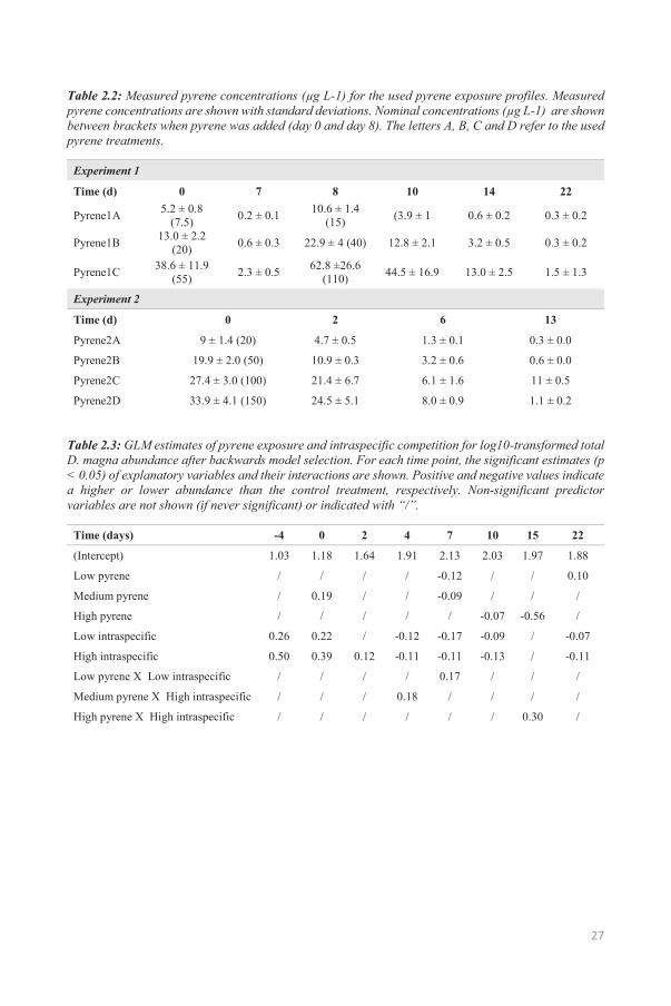
Measured pyrene concentrations in water were lower than expected from the nominal values (Table 2.2).
Nevertheless, there was a clear difference between the three pyrene exposure profiles at any given point
in time. The EcoDyna model was used to simulate pyrene concentration variations in water. The model
was run to fit actual water concentrations, and the importance of the main fluxes dominating the change
in concentration with time after the spikes. As a result of the fitting procedure, it was found that a
chemical half-life in water of 30 h was necessary to reproduce the observed concentrations (no
distinction could be made between biotic and abiotic processes), while volatilization accounted for about
20% of losses. Simulations confirmed that pyrene uptake in algae and animal biomass was negligible.
2.3.2. Population dynamics in absence of pyrene and interactions
Independent of the explanatory variables, a clear trend in the model intercept value could be observed.
In experiment 1, there was an increase in the intercept until day 7, afterwards the intercept slowly
decreased (Table 2.3-2.5). Similarly, in experiment 2 there was a strong population increase the first 14
days, followed by a slow decrease (Table 2.4). The intercept is the value estimated by the GLMs without
any effect of the predictor variables (pyrene and species interactions) and thus reflects the population
dynamics of D. magna without stress. The initial increase and then the decline of the intercept indicated
that the population was growing until the carrying capacity was reached (Figure 2.1).
27
Table 2.2: Measured pyrene concentrations (μg L-1) for the used pyrene exposure profiles. Measured pyrene concentrations are shown with standard deviations. Nominal concentrations (μg L-1) are shown between brackets when pyrene was added (day 0 and day 8). The letters A, B, C and D refer to the used pyrene treatments.
Experiment 1
Time (d) 0 7 8 10 14 22
Pyrene1A 5.2 ± 0.8 (7.5) 0.2 ± 0.1 10.6 ± 1.4
(15) (3.9 ± 1 0.6 ± 0.2 0.3 ± 0.2
Pyrene1B 13.0 ± 2.2 (20) 0.6 ± 0.3 22.9 ± 4 (40) 12.8 ± 2.1 3.2 ± 0.5 0.3 ± 0.2
Pyrene1C 38.6 ± 11.9 (55) 2.3 ± 0.5 62.8 ±26.6
(110) 44.5 ± 16.9 13.0 ± 2.5 1.5 ± 1.3
Experiment 2
Time (d) 0 2 6 13
Pyrene2A 9 ± 1.4 (20) 4.7 ± 0.5 1.3 ± 0.1 0.3 ± 0.0
Pyrene2B 19.9 ± 2.0 (50) 10.9 ± 0.3 3.2 ± 0.6 0.6 ± 0.0
Pyrene2C 27.4 ± 3.0 (100) 21.4 ± 6.7 6.1 ± 1.6 11 ± 0.5
Pyrene2D 33.9 ± 4.1 (150) 24.5 ± 5.1 8.0 ± 0.9 1.1 ± 0.2
Table 2.3: GLM estimates of pyrene exposure and intraspecific competition for log10-transformed total D. magna abundance after backwards model selection. For each time point, the significant estimates (p < 0.05) of explanatory variables and their interactions are shown. Positive and negative values indicate a higher or lower abundance than the control treatment, respectively. Non-significant predictor variables are not shown (if never significant) or indicated with “/”.
Time (days) -4 0 2 4 7 10 15 22
(Intercept) 1.03 1.18 1.64 1.91 2.13 2.03 1.97 1.88
Low pyrene / / / / -0.12 / / 0.10
Medium pyrene / 0.19 / / -0.09 / / /
High pyrene / / / / / -0.07 -0.56 /
Low intraspecific 0.26 0.22 / -0.12 -0.17 -0.09 / -0.07
High intraspecific 0.50 0.39 0.12 -0.11 -0.11 -0.13 / -0.11
Low pyrene X Low intraspecific / / / / 0.17 / / /
Medium pyrene X High intraspecific / / / 0.18 / / / /
High pyrene X High intraspecific / / / / / / 0.30 /
Chapter 2
28
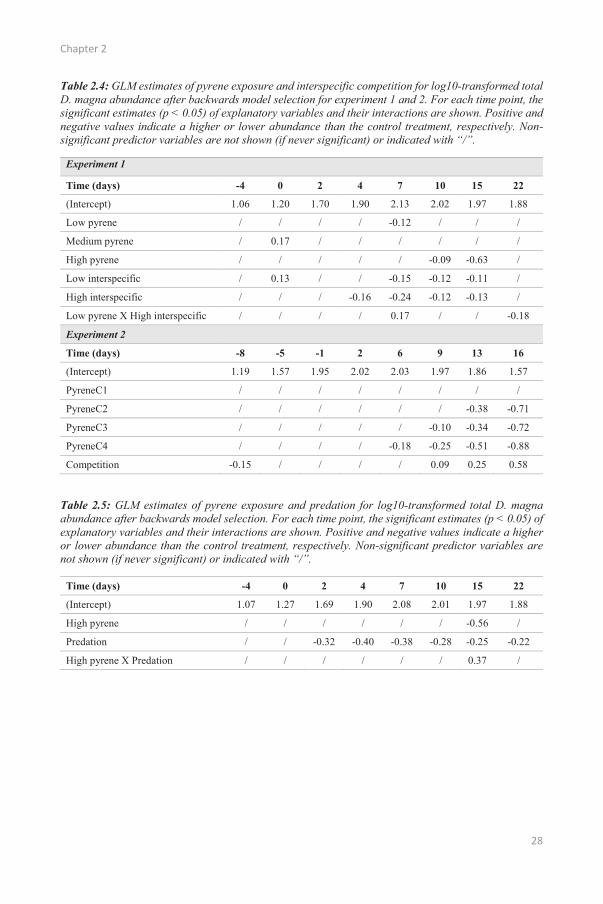
Table 2.4: GLM estimates of pyrene exposure and interspecific competition for log10-transformed total D. magna abundance after backwards model selection for experiment 1 and 2. For each time point, the significant estimates (p < 0.05) of explanatory variables and their interactions are shown. Positive and negative values indicate a higher or lower abundance than the control treatment, respectively. Non-significant predictor variables are not shown (if never significant) or indicated with “/”.
Experiment 1
Time (days) -4 0 2 4 7 10 15 22
(Intercept) 1.06 1.20 1.70 1.90 2.13 2.02 1.97 1.88
Low pyrene / / / / -0.12 / / /
Medium pyrene / 0.17 / / / / / /
High pyrene / / / / / -0.09 -0.63 /
Low interspecific / 0.13 / / -0.15 -0.12 -0.11 /
High interspecific / / / -0.16 -0.24 -0.12 -0.13 /
Low pyrene X High interspecific / / / / 0.17 / / -0.18
Experiment 2
Time (days) -8 -5 -1 2 6 9 13 16
(Intercept) 1.19 1.57 1.95 2.02 2.03 1.97 1.86 1.57
PyreneC1 / / / / / / / /
PyreneC2 / / / / / / -0.38 -0.71
PyreneC3 / / / / / -0.10 -0.34 -0.72
PyreneC4 / / / / -0.18 -0.25 -0.51 -0.88
Competition -0.15 / / / / 0.09 0.25 0.58
Table 2.5: GLM estimates of pyrene exposure and predation for log10-transformed total D. magna abundance after backwards model selection. For each time point, the significant estimates (p < 0.05) of explanatory variables and their interactions are shown. Positive and negative values indicate a higher or lower abundance than the control treatment, respectively. Non-significant predictor variables are not shown (if never significant) or indicated with “/”.
Time (days) -4 0 2 4 7 10 15 22
(Intercept) 1.07 1.27 1.69 1.90 2.08 2.01 1.97 1.88
High pyrene / / / / / / -0.56 /
Predation / / -0.32 -0.40 -0.38 -0.28 -0.25 -0.22
High pyrene X Predation / / / / / / 0.37 /

29
Figure 2.1. Total D. magna abundances over time for experiment 1 (A) with four pyrene exposure profiles and for experiment 2 (B) with five pyrene exposure profiles. Data shown are the D. magna population densities with no additional species interactions. Average values with standard deviations (error bars) are depicted. Dashed lines indicate pyrene applications.
(A)
(B)
Chapter 2
30
2.3.3. Effects of pyrene
For the first experiment, the estimated direct effects of pyrene were almost identical between the
different treatments of species interactions (Table 2.3-2.5). For experiment 1, I will therefore only refer
to Table 2.3 here. The first pyrene addition did not significantly affect D. magna population densities
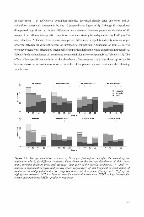
(Figure 2.1 and Table 2.3). However, the highest pyrene exposure did reduce total population densities
7 days after the second pyrene addition (day 15). The description and discussion of the experiment
results will therefore focus on the observed effects after the second pyrene addition. Effects of the
medium and low pyrene exposure profiles on total D. magna abundance were absent or negligible (<
0.13; Table 2.3). The variance of the total population densities explained by pyrene exposure at day 15
was >45% (Appendix A: Table A1-A3). Fourteen days after the second pyrene addition, D. magna
populations were recovering (day 22): no differences in total population densities were observed
between pyrene exposure profiles. However, at that time, the abundances of neonates were higher in the
high pyrene exposure profile than in the control treatment (Appendix A: Table A6 and Figure A2). Also,
the negative effect of high pyrene exposure on the abundances of adults persisted on day 22, although
this effect was smaller than on day 15 (Appendix A: Table A4). Although the total population densities
had recovered, differences in population structure were thus still observed between pyrene treatments
(Figure 2.1 and 2.2). In experiment 2, a similar delay in pyrene effect was observed (Figure 1B).
Significant negative effects were only observed 6 days after the pyrene addition (Table 2.4). Contrary
to experiment 1, significant negative effects were observed at the lower nominal pyrene concentrations.
Also, no recovery was observed at the end of experiment 2 and pyrene effects were visible at all size
classes (Appendix A: Table A13-A15).
2.3.4. Effects of interactions: competition and predation
During the first 9 days of the experiment, the populations with the higher initial population density of
40 individuals (and therefore a higher degree of intraspecific competition) remained more abundant but
this effect decreased with time (Figure 2.3 and Table 2.3). For the populations with an initial population
density of 20 individuals, this effect only persisted during the first 7 days. The variance explained by
intraspecific competition also decreased from 71% to 22% over this period (Appendix A: Table A1). A
high initial density resulted in lower future population densities (starting from day 4), although this
effect was limited (Table 2.3). The population with the lowest initial density (10 Daphnia per test vessel)
reached the highest total D. magna abundance (135 individuals). The initial positive effect of a high
initial density persisted longer for adult D. magna (until day 10; Appendix A: Table A4) than for the
other size classes (day 2 and -4 for juveniles and neonates, respectively; Appendix A: Table A5-A6).
High initial densities resulted in a higher and more constant abundance of adults in the second half of
the experiment compared to low initial densities (Figure 2.2).
31
In experiment 1, B. calyciflorus population densities decreased sharply after one week and B.
calyciflorus completely disappeared by day 10 (Appendix A: Figure A14). Although B. calyciflorus
disappeared, significant but limited differences were observed between population densities of D.
magna of the different interspecific competition treatments starting from day 4 until day 15 (Figure 2.4
and Table 2.4). At the end of the experimental period, differences in population density were no longer
observed between the different degrees of interspecific competition. Abundances of adult D. magna
were never negatively affected by interspecific competition during the whole experiment (Appendix A:
Table A7) while abundances of juvenile and neonate individuals were (Appendix A: Table A8-A9). The
effect of interspecific competition on the abundance of neonates was only significant up to day 10
because almost no neonates were observed in either of the pyrene exposure treatments the following
sample days.
Figure 2.2. Average population structure of D. magna just before and after the second pyrene application (day 8) for different treatments. Data shown are the average abundances of adults (dark grey), juveniles (medium grey) and neonates (light grey) of the specific treatments. “−“ and “+” indicate a significant negative and positive effect, respectively, of that treatment or combination of treatments on total population density, compared to the control treatment (“no pyrene”). High pyrene high pyrene exposure; INTRA = high intraspecific competition treatment; INTER = high interspecific competition treatment; PRED= predation treatment.
Chapter 2
32
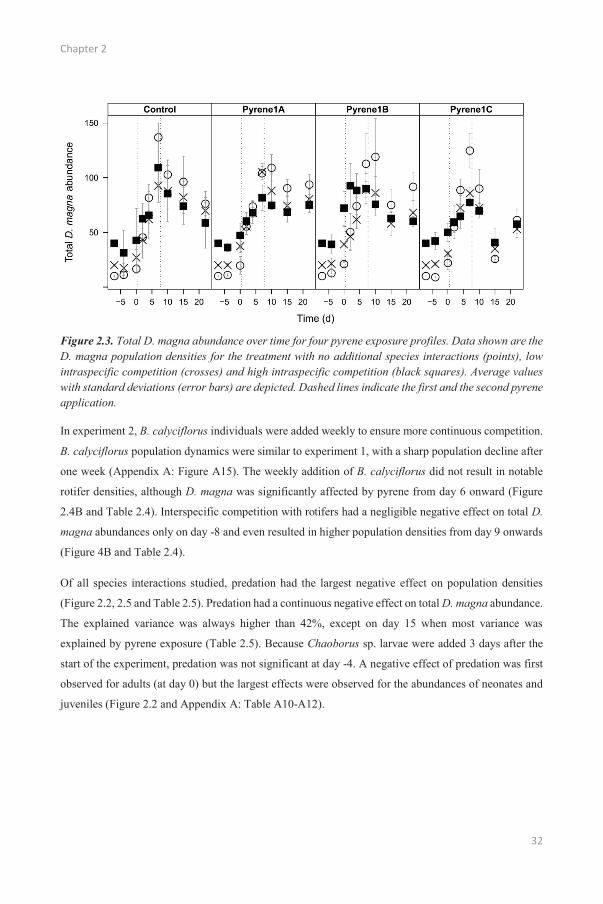
Figure 2.3. Total D. magna abundance over time for four pyrene exposure profiles. Data shown are the D. magna population densities for the treatment with no additional species interactions (points), lowintraspecific competition (crosses) and high intraspecific competition (black squares). Average valueswith standard deviations (error bars) are depicted. Dashed lines indicate the first and the second pyrene application.
In experiment 2, B. calyciflorus individuals were added weekly to ensure more continuous competition.
B. calyciflorus population dynamics were similar to experiment 1, with a sharp population decline after
one week (Appendix A: Figure A15). The weekly addition of B. calyciflorus did not result in notable
rotifer densities, although D. magna was significantly affected by pyrene from day 6 onward (Figure
2.4B and Table 2.4). Interspecific competition with rotifers had a negligible negative effect on total D.
magna abundances only on day -8 and even resulted in higher population densities from day 9 onwards
(Figure 4B and Table 2.4).
Of all species interactions studied, predation had the largest negative effect on population densities
(Figure 2.2, 2.5 and Table 2.5). Predation had a continuous negative effect on total D. magna abundance.
The explained variance was always higher than 42%, except on day 15 when most variance was
explained by pyrene exposure (Table 2.5). Because Chaoborus sp. larvae were added 3 days after the
start of the experiment, predation was not significant at day -4. A negative effect of predation was first
observed for adults (at day 0) but the largest effects were observed for the abundances of neonates and
juveniles (Figure 2.2 and Appendix A: Table A10-A12).
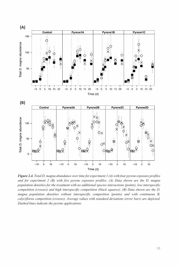
33
Figure 2.4. Total D. magna abundance over time for experiment 1 (A) with four pyrene exposure profiles and for experiment 2 (B) with five pyrene exposure profiles. (A) Data shown are the D. magna population densities for the treatment with no additional species interactions (points), low interspecific competition (crosses) and high interspecific competition (black squares); (B) Data shown are the D. magna population densities without interspecific competition (points) and with continuous B. calyciflorus competition (crosses). Average values with standard deviations (error bars) are depicted. Dashed lines indicate the pyrene applications.
(B)
(A)
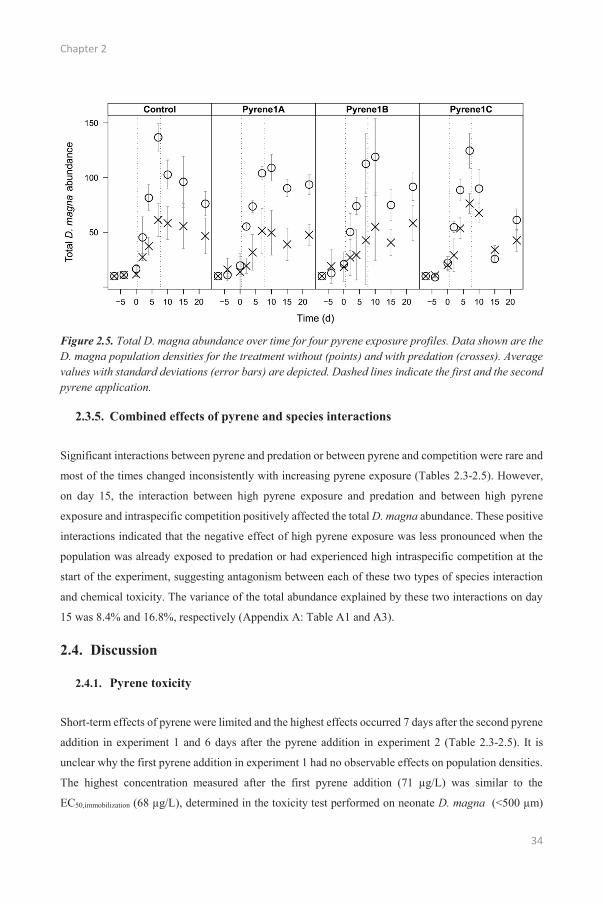
Chapter 2
34
Figure 2.5. Total D. magna abundance over time for four pyrene exposure profiles. Data shown are the D. magna population densities for the treatment without (points) and with predation (crosses). Average values with standard deviations (error bars) are depicted. Dashed lines indicate the first and the second pyrene application.
2.3.5. Combined effects of pyrene and species interactions
Significant interactions between pyrene and predation or between pyrene and competition were rare and
most of the times changed inconsistently with increasing pyrene exposure (Tables 2.3-2.5). However,
on day 15, the interaction between high pyrene exposure and predation and between high pyrene
exposure and intraspecific competition positively affected the total D. magna abundance. These positive
interactions indicated that the negative effect of high pyrene exposure was less pronounced when the
population was already exposed to predation or had experienced high intraspecific competition at the
start of the experiment, suggesting antagonism between each of these two types of species interaction
and chemical toxicity. The variance of the total abundance explained by these two interactions on day
15 was 8.4% and 16.8%, respectively (Appendix A: Table A1 and A3).
2.4. Discussion
2.4.1. Pyrene toxicity
Short-term effects of pyrene were limited and the highest effects occurred 7 days after the second pyrene
addition in experiment 1 and 6 days after the pyrene addition in experiment 2 (Table 2.3-2.5). It is
unclear why the first pyrene addition in experiment 1 had no observable effects on population densities.
The highest concentration measured after the first pyrene addition (71 μg/L) was similar to the
EC50,immobilization (68 μg/L), determined in the toxicity test performed on neonate D. magna (<500 μm)

35
from the same clone. However, even neonate D. magna – often considered the most sensitive individuals
(Muyssen and Janssen 2007) - were not affected by the first pyrene addition (Appendix A: Figure A10
and Table A6). The results of the pyrene toxicity test did thus not seem applicable to experiment 1.
It was unclear if the negative effects of pyrene on the abundances of adults after the second pyrene
addition resulted from direct mortality or from a combination of direct mortality and reduced survival
or growth of smaller life classes. Reduced survival and growth of earlier life stages will reduce the
number of juveniles that reach the adult stage (Liess and Foit 2010). The negative effect of pyrene was
largest on abundances of juveniles (Appendix A: Table A4-A6). Adult D. magna were the only size
class still affected by pyrene at the end of the experiment (Appendix A: Table 2.4). Probably, the
negative effect of pyrene on the abundances of adults was thus, at least partly, attributable to effects on
earlier life stages. Neonates were almost absent after the second pyrene addition, even in the control
treatment (Appendix A: Figure A10), which explains the absence of significant pyrene effects for
neonates. A low abundance of small individuals is not uncommon in similar experiments with Daphnia
(Preuss et al. 2009a) and can be attributed to the strong competition which reduces the energy available
for reproduction.
Interestingly, abundances of neonates were significantly higher on day 22 in the high pyrene exposure
profile than in the control treatment (Figure 2.2 and Appendix A: Table A6). As a result, total population
densities were not significantly different between the different pyrene treatments at the end of the
experiment (Table 2.3), leading to the conclusion that total population density was recovered. However,
it should be noted that the final D. magna populations in the high pyrene exposure profile, consisting
mainly of neonates, were probably more susceptible to new chemical stress events than those in the
other pyrene treatments. This illustrates that population structure needs to be accounted for when
assessing the response and recovery of a population to (chemical) stress (Foit et al. 2012).
In the follow-up experiment, measured pyrene concentrations were similar to the measured
concentrations of the first pyrene addition in the original experiment (Table 2.2). Nevertheless, this time
significant effects were observed, even in the lower pyrene concentrations (Table 2.4). It is unclear
whether this is the result of natural variation or of other factors such as the time of pyrene application.
The follow-up experiment was performed six months after the original experiment and it is possible
variations in environmental or biological conditions resulted in the observed differences in pyrene effect.
However, it is likely that the time of application was also an important factor: in the first experiment,
the pyrene was added when the population was growing and competition for resources between
individuals was limited. In the follow-up experiment, pyrene was added after 15 days, when the
population growth phase was already over. Competition for resources between D. magna individuals
was strong at this moment, possibly making the individuals less resistant to pyrene stress.
Chapter 2
36
Pyrene is a substance with low water solubility (0.132 mg L-1). Acetonitrile was used here as a solvent
to ensure that pyrene was dissolved in the water. Solvents are often used with pesticides to ensure a
solution that can easily be applied in the field. Solvents can possibly contribute to the toxicity of a
pesticide and it is therefore important to test the toxicity of the solvent itself. Acetonitrile was not toxic
to D. magna at the concentrations used here.
2.4.2. Species interactions
Of all species interactions studied, predation had the largest effect on total D. magna abundance. Effects
were visible six days after the addition of Chaoborus sp. larvae (starting from day 2) and the highest
effects were observed for the abundances of juveniles and neonates (Figure 2.2 and Appendix A: Table
A10-A12). This indicated a feeding preference: Chaoborus sp. larvae preferred to prey on smaller
juvenile and neonate D. magna than on adult D. magna. Size selective feeding by Chaoborus sp. larvae
has been observed before (Swift 1992). Surprisingly, however, a significant negative effect of predation
was first observed for adults (on day 0) and not for juveniles or neonates. Abundances of juveniles and
neonates were very low (juveniles) or zero (neonates) until day 0, so probably the Chaoborus larvae
were forced to feed on the larger D. magna adults. At later time points, neonates and juveniles were
more abundant and Chaoborus larvae fed on these size classes, leading to a reduced or absent effect of
predation on adults. These data show that feeding preferences depend on the ecological context shaped
by the prey’s population structure.
It is difficult to assess the effects of interspecific competition for the full duration of experiment 1
because B. calyciflorus were reduced to low densities (<10%) after day 7 and completely disappeared
after day 10 (Appendix A: Figure A14). The effects of interspecific competition on total population
densities were therefore limited (Table 2.3). Posterior tests performed with the same conditions showed
that even in the highest pyrene concentration, B. calyciflorus was able to survive for at least 24 days
(Appendix A: Figure A16). The rotifers were thus outcompeted by D. magna, as previously observed in
interaction experiments between B. calyciflorus and D. pulex without chemical stress (Gilbert 1985).
Gilbert et al. (1985) observed limited to no effects of the competition with B. calyciflorus on population
densities of D. pulex, similar to the results of the current chapter. In the follow-up experiment, B.
calyciflorus was added weekly but, even when D. magna was negatively affected by pyrene, notable
population densities of B. calyciflorus were not observed (Appendix A: Figure A15). Clearly, D. magna
was the superior competitor, even when exposed to the pyrene concentrations applied here.
Unexpectedly, weekly addition of rotifers had a positive effect on total D. magna population density in
the second half of experiment 2 (Table 2.4). To avoid the addition of additional algae, rotifers were
taken from the rotifer culture at least 24 hours after feeding. Nevertheless, it seems that algae and
possibly other nutrients were still present in high enough concentrations to positively influence D.
magna population abundances, masking any possible competition effect.
37
Both intraspecific and interspecific competition seemed to result in effects on reproductive output in
experiment 1. Negative effects of different initial densities on the abundances of neonates and juveniles
were observed starting from day 2 while these were absent for adults (Appendix A: Table A4-A6).
Similarly, negative effects of interspecific competition were observed for juveniles and neonates from
day 4 onward while adults were not affected (Appendix A: Table A7-A9). High initial competition thus
mainly affected early life stages at later time points, suggesting competition-induced effects on D.
magna reproduction over direct competition effects. According to the dynamic energy budget (DEB)
theory, the competition with B. calyciflorus or other D. magna individuals could reduce the amount of
energy that could be allocated to reproduction, resulting in less offspring (Kooijman 2010). However, it
is probable that direct competition, through starvation, also contributed to the results. Young D. magna
life stages are more prone to starvation than adults (Preuss et al. 2009a). Under high competition
conditions, less food is available per capita, possibly leading to starvation of smaller individuals and
contributing to the lower proportion of young life stages in the population.
2.4.3. Reduced effect of pyrene when combined with predation and competition
On day 15, when the pyrene effect was largest, predation and intraspecific competition reduced the
negative effect of pyrene on population densities (Figure 2.2). Contrary to the antagonism observed in
the current chapter, species interactions often lead to greater effects of chemical stress. For example, the
combination of predation by Notonecta maculata and exposure to nonylphenol led to loss of resilience
in Daphnia magna populations while individual stressors failed to affect population densities (Gergs et
al. 2013). Synergistic effects of competition and chemical stress have been reported for D. magna (Foit
et al. 2012) and other Daphnia species (Knillmann et al. 2012a). Next to synergistic effects, antagonistic
effects have been reported as well. For example, exposure to predator kairomones led to antagonistic
interactions with carbaryl exposure on reproduction of Daphnia magna (Coors and Meester 2008). This
was attributed to larger-sized and thus more tolerant offspring when predation cues were present. Two
mechanisms are proposed to explain the antagonism observed in the current chapter: differences in
population structure and pyrene-induced alterations in species interactions. First, the structure of the
populations exposed to predation or to high intraspecific competition differed from that of the
populations experiencing low intraspecific competition and populations not exposed to predation. On
day 7, immediately before the second pyrene addition, a large negative effect of intraspecific
competition and predation on the abundances of juveniles and neonates was observed while the
abundances of adults were less affected (Figure 2.2, Appendix A: Table A4-A6;A10-A12). Differences
in sensitivity for different D. magna size classes have been shown before e.g. for four metals (Hoang
and Klaine 2007) or carbaryl (Coors and Meester 2008). Because of the lower proportion of small-sized
and thus more sensitive life stages in populations with predation or high (initial) intraspecific
competition, pyrene effects were smaller. Second, the feeding rate of Chaoborus sp. larvae was possibly

Chapter 2
38
inhibited by the pyrene exposure, leading to reduced predation losses. Indeed, the estimated effect of
predation (Table 2.5) was lower on day 15. The effect of pyrene on the feeding rates of Chaoborus sp.
larvae was not tested in the current chapter but chemicals have been shown to alter feeding behaviour
of fish (Weis et al. 2001) and invertebrates (Maltby and Hills 2008).
Contrary to a similar study with D. magna populations exposed to fenvalerate (Liess and Foit 2010), we
observed no prolonged dominance of smaller-sized organisms after chemical stress in the treatment with
predation: after high pyrene exposure, the proportion of small individuals was higher in the populations
not exposed to predation (Figure 2.2). These contradicting results can be explained by differences in
how predation was applied in the two studies. While Liess and Foit (2010) simulated predation by
removing individuals non-selective on size, Chaoborus sp. larvae preferred to prey on smaller
individuals, leading to lower abundances of neonates in the predation treatments at the end of the
experiment. This highlights the complexity of assessing how ecological interactions alter the response
of a population to chemical stress and the need for ecologically realistic tools (De Laender and Janssen
2013; Gabsi et al. 2014b).
The results presented in the current chapter present an example of how species interactions can lead to
a priori unpredictable effects of chemicals. Predation and intraspecific competition were shown to
interact antagonistically with pyrene when the effect of pyrene was most pronounced. The current
chapter also highlights the need to not only consider the effects of a chemical on population density but
also on population structure when assessing the risk of chemicals for populations and communities.
Although the complexity of the interactions studied in this chapter was limited to interactions between
two species (competitors or predator-prey), this can yield significant insights that are applicable to more
complex food webs. Studies such as this chapter, in combination with approaches such as mechanistic
ecological models (De Laender et al. 2008b; Bontje et al. 2009; Galic et al. 2010), could be used to
integrate species interactions while assessing the long-term ecological risk of a chemical. Using
mechanistic ecological models will increase our understanding on how and when species interactions
influence the effects of a chemical. This will help identify in which situations species interactions are
an important factor for the ecological risk of a chemical and thus when special attention from the
regulators for species interactions is required.

39
3 DEVELOPMENT OF THE DEBKISS IBM
Redrafted from:
Viaene KPJ, De Laender F, Janssen CR, Baveco JM, Van den Brink PJ, Focks A. DEBkiss IBMs as a
novel tool to assess the population-level effects of chemicals on competing species. Submitted

Chapter 3
40
Abstract
Ecological models, in particular individual-based models (IBMs) have been suggested as a way forward
for the ecological risk assessment of chemicals. Most ecotoxicological tests focus on the individual level
and IBMs are ideal tools to translate these test results to the population and community level but need
to be based on a sound theoretical basis. Dynamic energy budget theory based on the keep it simple,
stupid principle (DEBkiss) offers a good compromise between complexity and the amount of data
required to parameterize the model. In this chapter, DEBkiss theory is presented and implemented with
an IBM to describe the life cycle of a generic organism. To account for the effects of chemicals, two
possible toxicity models were implemented: concentration-response curves and toxicokinetic
toxicodynamic models.

DEBkiss IBM development
41
3.1. Introduction
In Chapter 2, I have shown that interactions with other species can be important for population-level
effects in a community context. In the current chapter I will lay the foundations of a food-web model
based on IBMs. To this end, I present an novel and parameter sparse approach to individual-based
modelling based on the DEBkiss theory (Figure 3.1).
Figure 3.1: Overview of the DEBkiss IBM implementation. DEBkiss theory is used to model individual-level processes (see 3.3). An IBM is used to model all individuals in the population and derive population properties (see 3.4). The effects of chemical exposure are modelled using either concentration-response (CR) curves or toxicokinetic-toxicodynamic (TKTD) models (see 3.5).
3.2. Modelling species interactions under chemical stress
The complexity of species interactions makes it difficult to predict population-, community-, and
ecosystem-level effects of chemicals from single-species ecotoxicological tests. Therefore, ecological
models have been used to understand and predict the effects of chemicals on populations (De Laender
et al. 2008b; Galic et al. 2010), communities (De Laender et al. 2014b), and ecosystems (De Laender et
al. 2015). Models can help to test hypotheses regarding the relationship between effects occurring at
lower and higher levels of biological organisation. When based on solid mechanistic understanding, they
can be used to perform experiments in silico. Individual based models (IBMs) seem particularly suited
for use in ERA because population parameters and dynamics emerge from the mechanisms at the
individual level on which most ecotoxicological tests focus (Martin et al. 2013b). IBMs thus allow
exploring how individual-level effects extrapolate to higher levels of organisation (Galic et al. 2014;
Martin et al. 2014). In recent years, IBMs have been used to predict chemical effects on the population
dynamics of a number of typical test species used in ecotoxicology e.g. Daphnia magna (Martin et al.
2013a) and Asellus aquaticus (Galic et al. 2012). However, these IBM applications have focused solely
on the population level and not at higher levels of organisation.
IBMs need a theory describing the underlying individual-level processes. The dynamic energy budget
theory (DEB) was proposed as a suitable underlying theory for the individual level energy balance in
IBMs because this theory provides mechanistic understanding of patterns in growth, reproduction and

Chapter 3
42
mortality of individuals, and enables determination of species-specific parameters (Martin et al. 2013b).
One of the main challenges of standard DEB theory is the number of parameters and the type of
experiments required to accurately parameterize the model (Jager et al. 2013). For many species, these
are not available and the standard DEB model can thus not be parameterized. Also, DEB has some
shortcomings considering its use in a regulatory context: the equations in the standard DEB model can
be difficult to grasp and implementation in software is not straightforward. Therefore, a simplified
version of DEB, DEBkiss, following the paradigm of “keep it simple, stupid” and using less equations
and parameters, has been proposed to allow more transparency, reduce the amount of data required and
increase the user-friendliness (Jager et al. 2013). In DEBkiss, the parameters are more easy to interpret
and they can be more readily related to easily measured endpoints such as the maximum length or the
individual growth rate (Jager et al. 2013). Therefore, DEBkiss IBMs could be a useful tool for species
for which data are sparse.
When IBMs are used to predict the effects of chemicals, the individual-level (physiological) processes
that are sensitive to chemical stress need to be defined. Chemicals can interfere with physiological
processes in many ways. Even in a simplified DEB model, possible physiological modes of action
include effects on assimilation, maintenance and reproduction (Jager and Zimmer 2012). To determine
the actual physiological mode of action of a chemical, ideally full life-cycle studies are used (Jager and
Zimmer 2012). However, when data availability is limited, one is often forced to focus solely on the
effects of a chemical on individual survival. This drastically simplifies the model but also eases its
parameterization because data are more abundant. For example, the General Unified Threshold model
for Survival (GUTS) can be parameterized based on the results of simple acute toxicity tests (Jager et
al. 2011). GUTS is a generalization of a large range of existing toxicokinetic-toxicodynamic (TKTD)
models i.e. models that simulate the time course of processes leading to toxic effects. These models have
the advantage over the often-used concentration-effect equations that they can predict toxic effects even
when exposure is not constant. This allows them to be used in more realistic conditions, when exposure
to a chemical is not constant but changes over time.
3.3. DEBkiss theory
The dynamic energy budget (DEB) theory was originally developed in the ‘80s (Kooijman and Metz
1984) but only became widely applied for making sense of ecotoxicological studies during the past
decade (Kooijman 2010; Jager and Zimmer 2012). In DEB theory, all processes and states of an
individual are expressed as energy (or mass). Next, an energy (or mass) balance for the individual is
created (Kooijman 2010). DEB models describe processes at the level of the individual because,
compared to sub- and supra-individual levels of biological organization, it is relatively easy to make
energy and mass balances at the individual level (Kooijman 2010). DEB models use differential
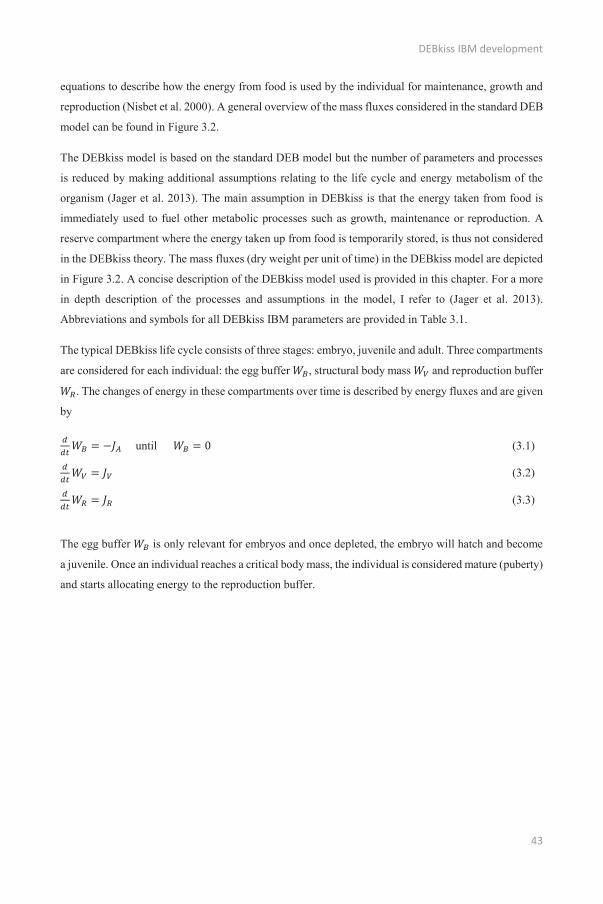
DEBkiss IBM development
43
equations to describe how the energy from food is used by the individual for maintenance, growth and
reproduction (Nisbet et al. 2000). A general overview of the mass fluxes considered in the standard DEB
model can be found in Figure 3.2.
The DEBkiss model is based on the standard DEB model but the number of parameters and processes
is reduced by making additional assumptions relating to the life cycle and energy metabolism of the
organism (Jager et al. 2013). The main assumption in DEBkiss is that the energy taken from food is
immediately used to fuel other metabolic processes such as growth, maintenance or reproduction. A
reserve compartment where the energy taken up from food is temporarily stored, is thus not considered
in the DEBkiss theory. The mass fluxes (dry weight per unit of time) in the DEBkiss model are depicted
in Figure 3.2. A concise description of the DEBkiss model used is provided in this chapter. For a more
in depth description of the processes and assumptions in the model, I refer to (Jager et al. 2013).
Abbreviations and symbols for all DEBkiss IBM parameters are provided in Table 3.1.
The typical DEBkiss life cycle consists of three stages: embryo, juvenile and adult. Three compartments
are considered for each individual: the egg buffer , structural body mass and reproduction buffer
. The changes of energy in these compartments over time is described by energy fluxes and are given
by
until (3.1)
(3.2)
(3.3)
The egg buffer is only relevant for embryos and once depleted, the embryo will hatch and become
a juvenile. Once an individual reaches a critical body mass, the individual is considered mature (puberty)
and starts allocating energy to the reproduction buffer.

Chapter 3
44
Fig
ure
3.2:
Gen
eral
sch
eme
of th
e en
ergy
flux
es c
onsi
dere
d in
the
stan
dard
DEB
mod
el (A
) and
in th
e D
EBki
ss m
odel
(B).
(A) I
n th
e st
anda
rd
DEB
mod
el, e
nerg
y fr
om fo
od is
take
n up
(X) a
nd a
ssim
ilate
d in
the
rese
rve
com
part
men
t (A)
. Ene
rgy
from
the
rese
rve
is m
obili
sed
(C) t
o fu
el
som
ati c
mai
nten
ance
(S),
grow
th (G
), m
atur
ity m
aint
enan
ce (J
) and
repr
oduc
tion
(R).
(B) I
n th
e D
EBki
ss m
odel
, ene
rgy
ente
rs th
e in
divi
dual
via
th
e fe
edin
g flu
x (J
X) o
r fro
m th
e eg
g bu
ffer i
f bir
th (b
) has
not
yet
occ
urre
d. T
he a
ssim
ilatio
n flu
x JA
is d
ivid
ed in
a fr
actio
n fo
r gro
wth
(flu
x JV
to
str
uctu
re) a
nd s
omat
ic m
aint
enan
ce (J
M) a
nd a
frac
tion
for
mat
urat
ion
and
repr
oduc
tion
(flux
JR
to th
e re
prod
uctio
n bu
ffer)
, dep
ende
nt o
n w
heth
er p
uber
ty (p
) has
occ
urre
d.

DEBkiss IBM development
45
Table 3.1: DEBkiss IBM model parameters. Primary parameters refer to parameters that are directly linked to the physiological processes and that do not depend on other parameters. Secondary parameters are determined by one or more primary parameters.
Symbol Parameter Unit
Primary parameters
Maximum specific searching rate L mm-2 d-1
Maximum specific assimilation rate mg dw mm-2 d-1
Volume-specific maintenance costs mg dw mm-3 d-1
Assimilates in a single freshly laid egg mg dw
Structural body mass at puberty mg dw
Yield of structure on assimilates (growth) -
Yield of assimilates on structure (starvation) -
Yield for conversion of reproduction buffer to eggs -
Yield of assimilates on food -
Fraction of assimilates for growth and maintenance -
Conversions
Dry-weight density of structure mg mm-3
Shape correction coefficient -
Fluxes and states
Mass flux for assimilation mg dw d-1
Mass flux for maintenance mg dw d-1
Mass flux for reproduction buffer mg dw d-1
Mass flux for structure mg dw d-1
Mass flux of food mg dw d-1
Mass of egg mg dw
Mass of reproduction buffer mg dw
Mass of structural body mg dw
X Food biomass mg dw L-1
Secondary parameters
f Scaled functional response (0-1) -
Maximum area-specific feeding rate mg dw mm-2 d-1
K Half-saturation food density mg dw L-1
L Volumetric body length mm
Maximum volumetric length mm
Physical body length mm
Von Bertalanffy growth rate constant d-1
ΔR Number of eggs in a clutch number of eggs
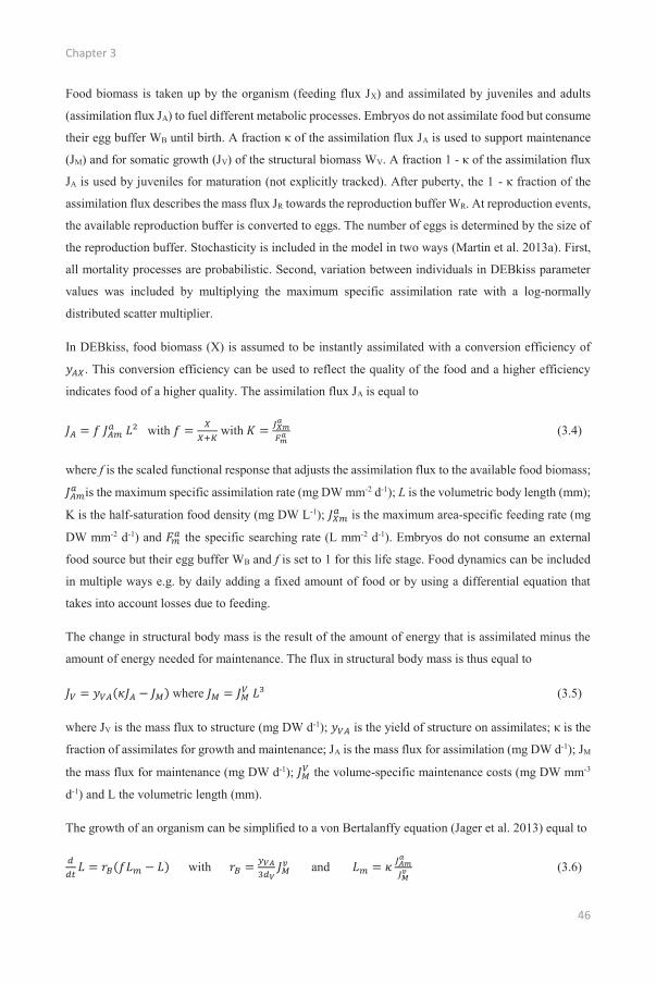
Chapter 3
46
Food biomass is taken up by the organism (feeding flux JX) and assimilated by juveniles and adults
(assimilation flux JA) to fuel different metabolic processes. Embryos do not assimilate food but consume
their egg buffer WB until birth. A fraction κ of the assimilation flux JA is used to support maintenance
(JM) and for somatic growth (JV) of the structural biomass WV. A fraction 1 - κ of the assimilation flux
JA is used by juveniles for maturation (not explicitly tracked). After puberty, the 1 - κ fraction of the
assimilation flux describes the mass flux JR towards the reproduction buffer WR. At reproduction events,
the available reproduction buffer is converted to eggs. The number of eggs is determined by the size of
the reproduction buffer. Stochasticity is included in the model in two ways (Martin et al. 2013a). First,
all mortality processes are probabilistic. Second, variation between individuals in DEBkiss parameter
values was included by multiplying the maximum specific assimilation rate with a log-normally
distributed scatter multiplier.
In DEBkiss, food biomass (X) is assumed to be instantly assimilated with a conversion efficiency of
. This conversion efficiency can be used to reflect the quality of the food and a higher efficiency
indicates food of a higher quality. The assimilation flux JA is equal to
with with (3.4)
where f is the scaled functional response that adjusts the assimilation flux to the available food biomass;
is the maximum specific assimilation rate (mg DW mm-2 d-1); L is the volumetric body length (mm);
K is the half-saturation food density (mg DW L-1); is the maximum area-specific feeding rate (mg
DW mm-2 d-1) and the specific searching rate (L mm-2 d-1). Embryos do not consume an external
food source but their egg buffer WB and f is set to 1 for this life stage. Food dynamics can be included
in multiple ways e.g. by daily adding a fixed amount of food or by using a differential equation that
takes into account losses due to feeding.
The change in structural body mass is the result of the amount of energy that is assimilated minus the
amount of energy needed for maintenance. The flux in structural body mass is thus equal to
where (3.5)
where JV is the mass flux to structure (mg DW d-1); is the yield of structure on assimilates; κ is the
fraction of assimilates for growth and maintenance; JA is the mass flux for assimilation (mg DW d-1); JM
the mass flux for maintenance (mg DW d-1); the volume-specific maintenance costs (mg DW mm-3
d-1) and L the volumetric length (mm).
The growth of an organism can be simplified to a von Bertalanffy equation (Jager et al. 2013) equal to
with and (3.6)

DEBkiss IBM development
47
where L is the volumetric length (mm); rB the von Bertalanffy growth constant (d-1); is the yield of
structure on assimilates; dV the dry-weight density of structure; the volume-specific maintenance
costs (mg DW mm-3 d-1); Lm the maximum volumetric length an individual can obtain (mm); κ is the
fraction of assimilates for growth and maintenance; is the maximum specific assimilation rate (mg
DW mm-2 d-1) and the volume-specific maintenance costs (mg DW mm-3 d-1).
The (1 – κ) fraction of the assimilation flux JA is used for maturation when the individual is juvenile
( ) or for the reproduction buffer when the individual is mature. The dynamics of the mass in
the reproduction buffer JR (mg DW d-1) are described by
(3.7)
where κ is the fraction of assimilates for growth and maintenance and JA the mass flux for assimilation.
At reproduction events, the available reproduction buffer is transformed into a number of eggs ( )
equal to
(3.8)
where is the yield for conversion of reproduction buffer to eggs; floor indicates that the lowest
whole number made possible by the division is selected; WR the mass of the reproduction buffer (mg
DW) and WB0 the egg mass (mg DW).
A special set of rules was used in the case of starvation (Jager et al. 2013). Initially, the energy shortage
is taken from the reproduction buffer (if any). In a second phase of starvation, the energy needed is
translated from the structural biomass and the organism shrinks. If an organism shrinks to a critical
fraction of its maximal attained weight, it has a high chance (0.35 d-1) of dying.
first stage: if but or
(3.9)
(3.10)
second stage: if and and
(3.11)
(3.12)
where κ is the fraction of assimilates for growth and maintenance; JA the mass flux for assimilation (mg
DW mm-2 d-1); JM the mass flux for maintenance (mg DW mm-2 d-1); WR the mass of the reproduction
buffer (mg DW); JV the mass flux for structure (mg DW mm-2 d-1) and the yield of assimilates on
structure (starvation).
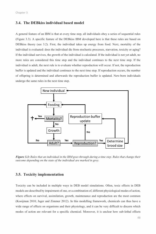
Chapter 3
48
3.4. The DEBkiss individual based model
A general feature of an IBM is that at every time step, all individuals obey a series of sequential rules
(Figure 3.3). A specific feature of the DEBkiss IBM developed here is that these rules are based on
DEBkiss theory (see 3.2). First, the individual takes up energy from food. Next, mortality of the
individual is evaluated: does the individual die from stochastic processes, starvation, toxicity or aging?
If the individual survives, the growth of the individual is calculated. If the individual is not yet adult, no
more rules are considered this time step and the individual continues to the next time step. If the
individual is adult, the next rule is to evaluate whether reproduction will occur. If not, the reproduction
buffer is updated and the individual continues to the next time step. If reproduction occurs, the number
of offspring is determined and afterwards the reproduction buffer is updated. New-born individuals
undergo the same rules in the next time step.
Figure 3.3: Rules that an individual in the IBM goes through during a time step. Rules that change their outcome depending on the state of the individual are marked in grey.
3.5. Toxicity implementation
Toxicity can be included in multiple ways in DEB model simulations. Often, toxic effects in DEB
models are described by impairment of one, or a combination of, different physiological modes of action,
where effects on survival, assimilation, growth, maintenance and reproduction are the most common
(Kooijman 2010; Jager and Zimmer 2012). In this modelling framework, chemicals can thus have a
wide range of effects on organisms and their physiology, and it can be very difficult to discern which
modes of action are relevant for a specific chemical. Moreover, it is unclear how sub-lethal effects

DEBkiss IBM development
49
translate to the population level. Consistent with the philosophy of DEBkiss, a simplified approach was
implemented where only effects on survival were considered. Two approaches to predict the effects of
a chemical on survival were evaluated: concentration-response (CR) relationships and toxicokinetic-
toxicodynamic (TKTD) models.
3.5.1. Concentration-response relationships
CR relationships give a straightforward relationship between the concentration of the chemical in the
water and the survival probability of an individual, based on standard toxicity test results. The survival
probability for a given time period (e.g. one day) can be predicted from the water concentration by
(3.13)
which only includes the concentration of the chemical in the water ( ) and two chemical-specific
parameters: the slope parameter and the of the chemical.
3.5.2. Toxicokinetic-toxicodynamic models
The TKTD model used is based on the general unified threshold model for survival (GUTS) which
offers a general framework for the wide variety of TKTD models available (Jager et al. 2011). In short,
toxicokinetic-toxicodynamic models predict the internal concentration over time from a given external
concentration (toxicokinetics) and link this internal concentration to a toxic effect at the level of the
individual over time (toxicodynamics) (Jager et al. 2011). The implemented TKTD model is based on
the reduced GUTS-SD model, assuming stochastic death and using a scaled internal concentration
(Figure 3.4). The GUTS-IT model, assuming the individual tolerance concept, was also implemented
but was sub-optimal for the species and chemical used here when applied to standard toxicity
experiments.
Figure 3.4: The implemented TKTD model. The dominant rate constant (kD1) describes the rate at which a chemical is taken up by the individual (C*int) from the environment (Cext). The killing rate constant (kk) and the internal threshold for effects (z) are used to link the scaled internal concentration (C*int) to a survival probability over time.
The TKTD model is described by three parameters: the dominant rate constant kD, the killing rate
constant kK and the internal threshold for effects z. To calculate the internal concentration of a chemical
(toxicokinetics), a first-order one-compartment model can often be used:

Chapter 3
50
(3.14)
where Cint is the internal concentration (μg kg-1); t is the time (d), kI is the uptake rate constant (L kg-1 d-
1); Cext the external concentration (μg -1) and kE the elimination rate constant (d-1). However, in
ecotoxicological studies, the internal concentration is mostly not measured. The GUTS model can still
be parameterized then by rescaling equation (3.14) and dividing both sides by kI/kE. This way, the
rescaled internal concentration C*int is directly proportional to the actual internal concentration and has
the dimensions of the external concentration:
(3.15)
where is the rescaled internal concentration (μg L-1); t is the time (d); kD is the dominant rate
constant and Cext the external concentration (μg -1). The elimination rate constant can be estimated from
the time-course of survival data even if internal concentrations are unknown. However, it is not
guaranteed that this estimated elimination rate constant represents only whole-body elimination. When
the elimination rate is estimated from only external concentration and survival data over time, the
slowest compensatory process, which can be either toxicokinetic (i.e. elimination from the body) or
toxicodynamic (i.e. recovery from damage), will dominate the dynamics of toxicity. Therefore, we refer
to the dominant rate constant kD instead of the elimination rate constant kE for the rescaled internal
concentration (Equation 3.15). To translate this rescaled internal concentration to effects on survival
over time, the cumulative hazard was used:
with (3.16)
where S(t) is the survival probability of an individual at time t; t is the time (d); HZ the cumulative hazard
of an individual at time t; kK the killing rate (L μg-1 d-1); selects the maximum of 0 and ;
is the rescaled internal concentration (μg L-1); z the internal threshold for effects (μg L-1) and hB the
background mortality rate (d-1).
Both toxicity approaches provide the probability, based on the chemical exposure, that an individual
will survive one more day. This survival probability is then evaluated for each individual in a population
to determine if it survives until the next day. The main difference between the two toxicity sub-models
is that CR relationships only consider the current chemical concentration and not earlier exposure while
chemical effects can still occur after exposure when using TKTD-SD.
3.6. Software
The DEBkiss IBM framework was implemented in NetLogo (Wilensky 1999), which was specifically
designed for IBMs and has been used before to implement DEB IBMs (Martin et al. 2012).

51
4 APPLICATION OF THE DEBKISS IBM FRAMEWORK TO
ASSESS THE EFFECTS OF COMPETITION AND CHEMICAL
STRESS ON THE POPULATION DYNAMICS OF
BRACHIONUS CALYCIFLORUS AND DAPHNIA MAGNA
Redrafted from:
Viaene KPJ, De Laender F, Janssen CR, Baveco JM, Van den Brink PJ, Focks A. DEBkiss IBMs as a
novel tool to assess the population-level effects of chemicals on competing species. In preparation.

Chapter 4
52
Abstract
To increase the ecological relevance of chemical risk assessment, the potential influence of species
interactions such as competition need to be accounted for. Ecological models have been identified as a
possible approach to consider species interactions, however, high data requirements often impair the
use of modelling approaches. Individual-based models based on a simplified dynamic energy budget
theory (DEBkiss IBMs) provide transparent and readily applicable models. In the current chapter, I
tested the capacity of an integrated model composed of two DEBkiss IBMs to predict the effects of pyrene
on two competing consumers, the cladoceran Daphnia magna and the rotifer Brachionus calyciflorus.
Both IBMs were calibrated using only data available in the literature and their performance was
evaluated using data from competition experiments. To predict the effects of pyrene, two possible toxicity
model implementations – concentration-response curves and toxicokinetic-toxicodynamic models – in
the IBMs were compared. Population dynamics of both species in isolation were reasonably well
predicted, although the population structure for D. magna was less well predicted. Agreeing with the
results of the experiments, D. magna outcompeted B. calyciflorus in the integrated model with both
species. The toxicokinetic-toxicodynamic model captured short-term effects of pyrene better than the
concentration-response model but overpredicted the chronic effects. Simulated rotifer population
dynamics exposed to both pyrene and competition were higher than those observed because of the
overprediction of pyrene effects on daphnid populations. Despite its limitations, the tested DEBkiss IBM
approach can be a useful tool for assessing the risk to species with short life cycles in case of low data
availability.

DEBkiss IBM application to experimental results
53
4.1. Introduction
Ecological models and especially individual-based models (IBMs) have received increasing attention in
ecotoxicology during the past decade. IBMs have been developed for several species such as Asellus
aquaticus (Galic et al. 2012), Daphnia magna (Preuss et al. 2009a) and Chaoborus (Dohmen et al.
2015). However, these models are still met with much scepticism by industry and regulators that are
unfamiliar with using models for effect assessment. In order to improve their use and acceptance, models
need to be validated (Grimm and Martin 2013; Grimm and Thorbek 2014). One common way to validate
models is to compare model output with patterns in available data. Patterns in this context are defined
as characteristics of the observations that are unlikely to be the result of random processes (Grimm and
Martin 2013). For complex systems, it is critical to evaluate multiple patterns because single patterns
can often be reproduced in multiple ways and it is then unknown whether the underlying mechanisms
are correctly captured. Key characteristics of complex ecological systems are interactions between
individuals of different species. Ecological models in general and IBMs more specifically that can
accurately predict how these interactions affect the population dynamics of the species involved,
especially in the context of chemical stress, could become essential tools in future ecological risk
assessment approaches.
The main objective of this chapter was therefore to test whether the DEBkiss IBM framework described
in Chapter 3 is suitable to simulate and understand patterns observed for two interacting populations
under chemical stress. To reach this objective, DEBkiss IBMs were implemented and parameterized for
two grazers (the water flea Daphnia magna and the rotifer Brachionus calyciflorus) and a framework
was developed to allow multiple DEBkiss IBMs to compete for a shared resource (the algae
Scenedesmus obliquus). Simulations were performed for the control treatment, for exposure to pyrene,
for interspecific competition, and for a combination of pyrene exposure and interspecific competition.
To evaluate the performance of the model for predicting the combination of ecological (competition)
and chemical stress, simulation results were compared to the patterns observed in the experiments
described in Chapter 2.
4.2. Materials and Methods
4.2.1. Model parameterization
Available literature data were used to determine a range of possible DEBkiss IBM parameter values
(Table 4.1). The available literature for Daphnia magna and Brachionus calyciflorus was queried for
DEB-related parameters such as maximum body lengths, growth rates, ingestion rates, egg weights and
length-weight relationships. Parameter values from other DEB models were avoided because these have
been fitted for more complex DEB models which differ from DEBkiss (e.g. by including a reserve
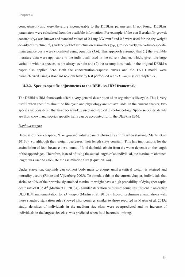
Chapter 4
54
compartment) and were therefore incomparable to the DEBkiss parameters. If not found, DEBkiss
parameters were calculated from the available information. For example, if the von Bertalanffy growth
constant ( ) was known and standard values of 0.1 mg DW mm-3 and 0.8 were used for the dry-weight
density of structure ( ) and the yield of structure on assimilates ( ), respectively, the volume-specific
maintenance costs were calculated using equation (3.6). This approach assumed that (1) the available
literature data were applicable to the individuals used in the current chapter, which, given the large
variation within a species, is not always certain and (2) the assumptions made in the original DEBkiss
paper also applied here. Both the concentration-response curves and the TKTD model were
parameterized using a standard 48-hour toxicity test performed with D. magna (See Chapter 2).
4.2.2. Species-specific adjustments to the DEBkiss-IBM framework
The DEBkiss IBM framework offers a very general description of an organism’s life cycle. This is very
useful when specifics about the life cycle and physiology are not available. In the current chapter, two
species are considered that have been widely used and studied in ecotoxicology. Species-specific details
are thus known and species specific traits can be accounted for in the DEBkiss IBM.
Daphnia magna
Because of their carapace, D. magna individuals cannot physically shrink when starving (Martin et al.
2013a). So, although their weight decreases, their length stays constant. This has implications for the
assimilation of food because the amount of food daphnids obtain from the water depends on the length
of the appendages. Therefore, instead of using the actual length of an individual, the maximum obtained
length was used to calculate the assimilation flux (Equation 3-4).
Under starvation, daphnids can convert body mass to energy until a critical weight is attained and
mortality occurs (Rinke and Vijverberg 2005). To simulate this in the current chapter, individuals that
shrink to 40% of their previously attained maximum weight have a high probability of dying (per capita
death rate of 0.35 d-1 (Martin et al. 2013a)). Similar starvation rules were found insufficient in an earlier
DEB IBM implementation for D. magna (Martin et al. 2013a). Indeed, preliminary simulations with
these standard starvation rules showed shortcomings similar to those reported in Martin et al. 2013a
study: densities of individuals in the medium size class were overpredicted and no increase of
individuals in the largest size class was predicted when food becomes limiting.

DEBkiss IBM application to experimental results
55
Bra
chio
nus c
alyc
iflor
us
[0.0
2 –
0.12
] * 1
0-3 m
g dw
(D
umon
t et a
l. 19
75; S
aund
ers I
II a
nd
Lew
isJr
1988
)[0
.15
– 0.
21] *
10-3
mg
dw a
[0.0
88 –
0.1
95] m
g dw
mm
-2 d
-1 a
[0.3
37 –
0.7
47] L
mm
-2 d
-1 a
0.76
47 m
g dw
mm
-3 d
-1 a
2.03
93 d
-1 a
[0.0
92 –
0.2
04] m
m a
0.32
6391
4 dw
L-1
(Han
sen
and
Bjo
rnse
n 19
97)
[0.6
-0.9
5] b
0.8 b
0.95
b
[0.6
-0.9
5] b
[0.4
– 0
.9] b
0.1
mg
dw m
m-3
a
0.50
97 a
0.5
d (H
alba
ch 1
970b
) 0.
8 a
0.01
d-1
a
10 d
(H
alba
ch 1
970b
)
Dap
hnia
mag
na
[7-1
0] *
10-3
mg
dw
(Dum
ont e
t al.
1975
; Till
man
n an
d La
mpe
rt 19
84;
Gla
zier
1992
)[0
.027
– 0
.031
5] m
g dw
a
[0.0
6 –
0.12
1] m
g dw
mm
-2 d
-1 a
[0.0
265
– 0.
6526
] L m
m-2
d-1
a
[0.0
4125
– 0
.051
] mg
dw m
m-3
d-1
a
0.13
7 d-1
(Pie
ters
et a
l. 20
06; J
ager
and
Zim
mer
201
2)
1.9
mm
a
[0.1
22 –
2.2
38] m
g dw
L-1
(Mul
der a
nd H
endr
iks 2
014)
0.8 b
0.8 b
0.95
b
0.8 b
[0.5
– 0
.9] b
0.1
mg
dw m
m-3
a
0.38
a
2.8
d a
0.4
a
0.02
d-1
a
96 d
(M
acA
rthur
and
Bai
llie
1929
)
Para
met
er
Ass
imila
tes i
n a
sing
le fr
eshl
y la
id e
gg
Stru
ctur
al b
ody
mas
s at p
uber
ty
Max
imum
spec
ific
assi
mila
tion
rate
Spec
ific
sear
chin
g ra
te
Vol
ume-
spec
ific
mai
nten
ance
cos
ts
Von
Ber
tala
nffy
gro
wth
rate
con
stan
t
Max
imum
vol
umet
ric le
ngth
Hal
f-sa
tura
tion
food
den
sity
Yie
ld o
f stru
ctur
e on
ass
imila
tes (
grow
th)
Yie
ld o
f ass
imila
tes o
n st
ruct
ure
(sta
rvat
ion)
Yie
ld fo
r con
vers
ion
of re
prod
uctio
n bu
ffer
to e
ggs
Yie
ld o
f ass
imila
tes o
n fo
od
Frac
tion
of a
ssim
ilate
s for
gro
wth
and
mai
nten
ance
Dry
-wei
ght d
ensi
ty o
f stru
ctur
e
Shap
e co
rrec
tion
coef
ficie
nt
Tim
e be
twee
n re
prod
uctio
n ev
ents
Bod
y m
ass f
ract
ion
at w
hich
star
vatio
n oc
curs
Stoc
hast
ic m
orta
lity
rate
Max
imum
age
of a
n in
divi
dual
Sym
bol
K
- - - -
Tabl
e 4.
1: P
aram
eter
val
ue r
ange
s fo
r D
. mag
na a
nd B
. cal
ycifl
orus
. a C
alcu
late
d us
ing
equa
tions
(3.4
) and
(3.6
). b
Sugg
este
d va
lues
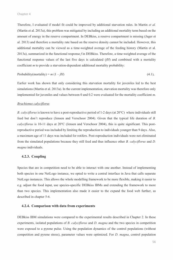
Chapter 4
56
Therefore, I evaluated if model fit could be improved by additional starvation rules. In Martin et al.
(Martin et al. 2013a), this problem was mitigated by including an additional mortality term based on the
amount of energy in the reserve compartment. In DEBkiss, a reserve compartment is missing (Jager et
al. 2013) and therefore a mortality rate based on the reserve density cannot be included. However, this
additional mortality can be viewed as a time-weighted average of the feeding history (Martin et al.
2013a), summarized in the functional response f in DEBkiss. Therefore, a time-weighted average of the
functional response values of the last five days is calculated (fH) and combined with a mortality
coefficient m to provide a starvation-dependent additional mortality probability:
Probability(mortality) = m (1 – fH) (4.1),
Earlier work has shown that only considering this starvation mortality for juveniles led to the best
simulations (Martin et al. 2013a). In the current implementation, starvation mortality was therefore only
implemented for juveniles and values between 0 and 0.2 were evaluated for the mortality coefficient m.
Brachionus calyciflorus
B. calyciflorus is known to have a post-reproductive period of 1-2 days (at 20°C) where individuals still
feed but don’t reproduce (Jensen and Verschoor 2004). Given that the typical life duration of B.
calyciflorus is 10-11 days at 20°C (Jensen and Verschoor 2004), this is quite significant. This post-
reproductive period was included by limiting the reproduction to individuals younger than 9 days. Also,
a maximum age of 11 days was included for rotifers. Post-reproduction individuals were not eliminated
from the simulated populations because they still feed and thus influence other B. calyciflorus and D.
magna individuals.
4.2.3. Coupling
Species that are in competition need to be able to interact with one another. Instead of implementing
both species in one NetLogo instance, we opted to write a central interface in Java that calls separate
NetLogo instances. This allows the whole modelling framework to be more flexible, making it easier to
e.g. adjust the food input, use species-specific DEBkiss IBMs and extending the framework to more
than two species. This implementation also made it easier to the expand the food web further, as
described in chapter 5-6.
4.2.4. Comparison with data from experiments
DEBkiss IBM simulations were compared to the experimental results described in Chapter 2. In these
experiments, isolated populations of B. calyciflorus and D. magna and the two species in competition
were exposed to a pyrene pulse. Using the population dynamics of the control populations (without
competition and pyrene stress), parameter values were optimized. For D. magna, control population

DEBkiss IBM application to experimental results
57
dynamics were available from two experiments (see Chapter 2) and both were used for parameter
optimization. To account for variation in the parameters, 100 simulations were performed with random
sampling from the range of possible DEBkiss parameter values given in Table 4.1. 100 simulations were
chosen because this was deemed a good compromise between computation time and accounting for the
variation on the DEBkiss parameters. Optimization was done by likelihood optimization (Jager and
Zimmer 2012) with the likelihood l of the parameter set θ given the data Y calculated as
where N is the total number of data points and SSQ the sum of squared residuals. The SSQ is given by
(4.3)
where i is the time point of the observation (from i to k), the estimated value for observation i using
parameter set θ and the observed value for observation i.
Population dynamics of the control treatments were used to select the 10 best (out of 100) parameter
combinations for each species based on the calculated likelihoods (Table 4.2). Because the size structure
of the population was important for the response to stress (Chapter 2), likelihoods for D. magna were
calculated for both the total density and the densities of the size classes. The likelihoods of the total
density and of the three size classes were then multiplied to derive one value to be optimized. By doing
so, the parameter combinations were selected that best described both the total population density and
the population structure. Initial exploration of the likelihoods showed that the maximum area-specific
assimilation rate ( ) was the dominant factor determining the likelihood, with the lowest likelihood
for high values (Appendix B Figure B1). Therefore, the range for was limited in the simulations to
values between 0.06 mg mm-2 d-1 and 0.121 mg mm-2 d-1. Extinction of B. calyciflorus in the control
treatment was observed by the end of the experiment (31 days), most likely due to abiotic causes e.g.
decreased water quality. Therefore, only the population densities of the control treatment of the first 22
days were used to fit the model.
Table 4.2: Steps, parameters and experiments used for the simulations in this Chapter.
Step Parameters used Related Chapter 2 experiment 1 100 random combinations of literature
parameter values (Table 4.1) Experiment 1: Control Experiment 2: Control
2 10 optimal parameter combinations from step 1 Experiment 2: Interspecific competition 3 10 optimal parameter combinations from step 1 Experiment 2: Pyrene 4 10 optimal parameter combinations from step 1 Experiment 2: Interspecific competition +
Pyrene

Chapter 4
58
The 10 optimal parameter combinations for both species were then used to predict the dynamics for
exposure to competition, exposure to pyrene and exposure to both competition and pyrene (Table 4.2).
When simulating two competing species, each of the 10 optimal parameter combination of D. magna
were combined with each of the 10 optimal parameter combination of B. calyciflorus, resulting in a total
of 100 simulations. To evaluate the effects of pyrene, both the concentration-response (CR) and the
toxicokinetic-toxicodynamic (TKTD) models were tested. Simulations were only compared to the data
of experiment 2 because it was unclear how exposure to two pyrene pulses, as was the case in experiment
1, affected the daphnids and if the toxicity models could capture this. In experiment 2, only one pyrene
addition was performed and the applicability of both toxicity models should be more clear. 100
simulations were run for the pyrene exposure to account for stochasticity. Simulations for exposure to
both competition and pyrene were also simulated 100 times. For all these treatments, the calculated
likelihoods were used again to select the 10 simulations (out of 100) closest to the observed densities.
4.3. Results
4.3.1. Daphnia magna
Figures 4.1-4.3 in the current chapter show the optimal fit of the DEBkiss IBMs i.e. the 10 best
simulations of the 100 simulations performed per treatment, based on the likelihood. Simulations of
isolated D. magna populations without chemical stress showed a population growth phase followed by
a decline as the carrying capacity of the system was reached (Figure 4.1). Despite differences in the
observed maximum population densities of the two experiments used for parameter optimization (150
individuals versus 110 individuals), the population trends in both experiments were similar (Figure 4.1).
The maximum density of the first experiment was predicted by some of the 100 performed simulations
but since the optimization was performed for all counted abundances, the best simulations shown in
Figure 4.1 are more in line with the maximum density counted in the second experiment. The maximum
population density in the simulations was lower and occurred earlier than in the experimental
observations. In the second half of the experiments, the simulated population density was therefore lower
than the observed density. The population densities at the end of the experiment were more comparable
between simulations and experiments (Figure 4.1).
The largest discrepancy between the control treatment of experiments and simulations was observed for
the abundance of large individuals at the end of the experiment (Appendix B Figure B2). While a steady
increase of large individuals was observed until the end of the experiment, a constant, low abundance
of large individuals was predicted. Related to this, the abundance of intermediate individuals strongly
decreased in the experiments while this was not observed in the simulations. A similar trend was
observed in an earlier study and was alleviated by including additional starvation mortality related to
the reserve density of an individual (Martin et al. 2013a). Because DEBkiss IBMs lack a reserve
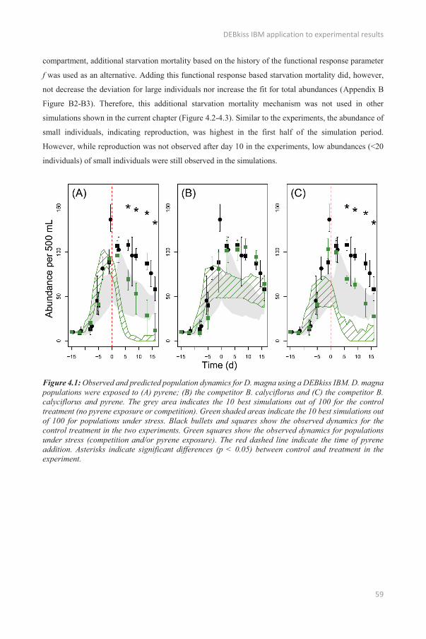
DEBkiss IBM application to experimental results
59
compartment, additional starvation mortality based on the history of the functional response parameter
f was used as an alternative. Adding this functional response based starvation mortality did, however,
not decrease the deviation for large individuals nor increase the fit for total abundances (Appendix B
Figure B2-B3). Therefore, this additional starvation mortality mechanism was not used in other
simulations shown in the current chapter (Figure 4.2-4.3). Similar to the experiments, the abundance of
small individuals, indicating reproduction, was highest in the first half of the simulation period.
However, while reproduction was not observed after day 10 in the experiments, low abundances (<20
individuals) of small individuals were still observed in the simulations.
Figure 4.1: Observed and predicted population dynamics for D. magna using a DEBkiss IBM. D. magna populations were exposed to (A) pyrene; (B) the competitor B. calyciflorus and (C) the competitor B. calyciflorus and pyrene. The grey area indicates the 10 best simulations out of 100 for the control treatment (no pyrene exposure or competition). Green shaded areas indicate the 10 best simulations out of 100 for populations under stress. Black bullets and squares show the observed dynamics for the control treatment in the two experiments. Green squares show the observed dynamics for populations under stress (competition and/or pyrene exposure). The red dashed line indicate the time of pyrene addition. Asterisks indicate significant differences (p < 0.05) between control and treatment in the experiment.

Chapter 4
60
Two toxicity models were evaluated, concentration-response curves (CR) and toxicokinetic-
toxicodynamic models with stochastic death (TKTD-SD; Figure 4.2). Effects of pyrene were only
considered for D. magna as no effects were observed for B. calyciflorus, neither in the acute toxicity
test (Chapter 2) nor in the population experiment (Figure 4.3). Using CR curves, pyrene effects occurred
immediately while a delay of a week was observed in the experiments (Figure 4.1). Also, D. magna
populations recovered after two weeks in the simulations while this was not observed in the experiment.
Using TKTD-SD, effects were more delayed (1-2 days) but still too fast. Also, the effects of pyrene
were larger, potentially even leading to extinction of the daphnid population, and persisted longer than
with the CR toxicity model (Figure 4.2). Both considered toxicity models were thus unable to fully
capture the effects of pyrene on D. magna population dynamics. Although the predicted effects of pyrene
were too high, the TKTD-SD model was preferred over the CR model because the slight delay in pyrene
effects and the absence of population recovery matched the observations most closely.
Figure 4.2: Comparison of the DEBkiss simulations for D. magna with concentration-response curve (A) or TKTD-SD (B) as toxic effect sub-model. The grey area indicates the 10 best simulations out of100 for the control treatment (no pyrene exposure or competition). Green shaded areas indicate the 10best simulations out of 100 for populations under stress. Black bullets and squares show the observeddynamics for the control treatment in the two experiments. Green squares show the observed dynamicsfor populations under stress (competition and/or pyrene exposure). The red dashed line indicates thetime of pyrene addition. Asterisks indicate significant differences (p < 0.05) between control andtreatment in the experiment.

DEBkiss IBM application to experimental results
61
4.3.2. Brachionus calyciflorus
Simulations for the isolated B. calyciflorus populations reflected the pattern of population increase and
decrease observed in the experiment (Figure 4.3). For B. calyciflorus, the simulated maximum total
population density was comparable to that observed in the experiments. Because pyrene effects were
not predicted for individuals at the measured pyrene concentrations, exposure to pyrene did not alter the
B. calyciflorus population dynamics.
Figure 4.3: Simulated population dynamics of B. calyciflorus using a DEBkiss IBM. B. calyciflorus populations were exposed to (A) pyrene; (B) competition with D. magna and (C) both competition with D. magna and pyrene exposure. The grey area indicates the 10 best simulations out of 100 for the control treatment (no pyrene exposure or competition). Green shaded areas indicate the 10 best simulations out of 100 for populations under stress. Black squares show the observed dynamics for the control treatment in the two experiments. Green squares show the observed dynamics for populations under stress (competition and/or pyrene exposure). The red dashed lines indicates the time of pyrene addition. Asterisks indicate significant differences (p < 0.05) between control and treatment in the experiment.
4.3.3. Competition
As observed in the experiments, daphnids were also the superior competitors in the simulations (Figure
4.1 and Figure 4.3). Simulated daphnid population dynamics were largely unaffected by competition
with rotifers, which corresponds to the experimental results. The only effects of competition on daphnid
populations were a 23% lower maximum population density and an earlier cessation of population
growth (five days earlier) in the competition treatment simulations than in the simulations of the control
treatment. However, differences between isolated populations and populations in competition with
rotifers were not observed in the experiment. Simulated population dynamics of B. calyciflorus
competing with D. magna corresponded well with experimental results (Figure 4.3): a population

Chapter 4
62
increase when food was not yet limiting – but lower than for isolated B. calyciflorus populations – and
a very low population abundance or extinction when food was scarce, although the population persisted
longer than observed.
4.3.4. Competition and chemical stress
When D. magna was exposed to both pyrene and competition, the effect of pyrene on D. magna was
unaltered: daphnid populations decreased, potentially leading to extinction (Figure 4.1). This was similar
to that observed in the experiments where the effect of pyrene showed no interaction with the effect of
interspecific competition (see Chapter 2). Contrary to the experiments, rotifers increased in abundance
after pyrene exposure (Figure 4.3).
4.4. Discussion
4.4.1. Predictive capability of DEBkiss IBM for Daphnia magna and Brachionus
calyciflorus
In general, the effects of food shortage on D. magna populations appeared sooner in the DEBkiss IBM
than in reality. Several deviations between the experiments and the simulations could be ascribed to the
absence of a reserve compartment in the D. magna DEBkiss IBM: compared to the experiments, the
simulations showed lower maximum population densities, earlier population decline, lower abundance
of large individuals and higher effects of competition with B. calyciflorus. The implementation of an
additional starvation mechanism similar to another D. magna DEB IBM implementation (Martin et al.
2013a) proved unsuccessful. The absence of a reserve compartment thus limits the application of the
DEBkiss IBM for conditions when the population is starving. The starvation recovery rules were also
lacking: while reproduction was not observed after day 10 in the experiments, low abundances (<20
individuals) of small individuals were still observed in the simulations. In the DEBkiss implementation,
starving individuals shrink to meet their energy needs. When food is available again, they immediately
spend a fixed part of the assimilated energy on reproduction. However, it seems unlikely that the
proportion of assimilated energy spent on reproduction is identical for well-fed individuals and
individuals recovering from starvation. Implementing starvation recovery rules that favour recovery of
weight over growth and reproduction could improve the fit of the simulations. However, many different
starvation recovery strategies have been proposed for D. magna and a general consensus is lacking
(Vanoverbeke 2008).
The instantaneous effects of pyrene on D. magna populations when modelling toxicity with CR curves
is not surprising given that only the current chemical concentration is used to predict pyrene effects.
There is thus no delay between exposure and effects possible, although a delay of about a week was

DEBkiss IBM application to experimental results
63
observed for pyrene. Similarly, effects of pyrene disappear quickly with the CR approach, explaining
the predicted recovery. The TKTD approach can account for a delay in effects and recovery but effects
were still too fast for the experiments used. A possible cause for the deviation between the effects
predicted by the toxicity models and the observed effects is that the parameterization of these models
was done using the result from an acute toxicity test performed with D. magna juveniles. Chronic
toxicity can differ from acute toxicity e.g. because of alternative modes of action or toxicity of the
biotransformation products (Dom et al. 2012). Also, the endpoint used in the D. magna toxicity test was
immobilization and it can take a few days for immobilized individuals to die. Moreover, the presence of
different size classes can influence the susceptibility of a population to toxic stress: larger D. magna
individuals have been shown to be more resistant to e.g. carbaryl (Coors and Meester 2008), possibly
explaining the observed delay in effect of pyrene at concentrations close to the acute EC50. Alternatively,
due to its assumed narcotic mode of action (Di Toro et al. 2000), it is possible that pyrene causes sub-
lethal effects in daphnids. Including such sub-lethal effects might explain the delayed effect of pyrene
on total population density. More complex toxicity models which e.g. consider effects on maintenance
costs or other modes of action were not tested because (1) the aim of the chapter was to test the efficacy
of a simple (toxicity) model and (2) accurate information about the mode of action of pyrene or different
sensitivity of life stages to pyrene is lacking.
The observed population decline of rotifers at the end of the experiment was most likely due to
unsuitable environmental conditions e.g. decreased water quality, waste accumulation and/or changed
physico-chemical parameters of the water, which are not considered in the IBMs. For example, the pH
decreased from 7.7 ± 0.1 at the start to 6.5 ± 0.3 at the end of the second experiment and the oxidation-
reduction potential increased over the same period from -61 ± 5 mV to 9 ± 16 mV. Other water quality
parameter and waste products were not measured in the experiments.
Competitive exclusion has been observed frequently for rotifers competing with daphnids (MacIsaac
and Gilbert 1989). We were able to simulate this exclusion and its effects on both species, although the
disappearance of rotifers was slower in the simulations than in the experiments. Possibly, other
mechanisms not considered here accelerated the extinction of rotifers e.g. rotifers can be damaged by
mechanical interference – rejection after accidental ingestion – with feeding daphnids (Gilbert 1988). It
is also plausible that such low abundances of B. calyciflorus were simply not detected in the experiments.
Because of the transparency and low complexity of the DEBkiss IBMs, it would be easy to implement
additional competition mechanisms for species when this is needed.
The predicted increase in rotifers after pyrene addition did not correspond with the experiments but is
logical when looking at the other simulations. This difference was caused by the rotifers still being
present in the simulations at the time of pyrene addition contrary to the experiments. Moreover, the
effect of pyrene on daphnids occurred much faster in the simulations than in the experiments, increasing
Chapter 4
64
the amount of algae available to rotifers. Also, some daphnid populations were completely eliminated
by pyrene, which resulted in improved B. calyciflorus growth conditions i.e. without competition for
food. In fact, if a similar pyrene effect had occurred on D. magna in the experiments as in the
simulations, an increase in B. calyciflorus in the experiments would be expected.
In general, population dynamics were accurately predicted using a DEBkiss IBM and the DEBkiss IBM
approach is especially applicable for organisms with short life cycles. Despite the limitations of the
DEBkiss IBM to capture the observed population dynamics and structure of D. magna exactly, the
endpoints that are most focused on in traditional ERA – population growth, total population density and
reproduction – were reasonably well predicted. Also, the toxicity models considered here do not account
for size-dependent effects, which limits the impact of a faulty population structure on the population
dynamics after toxic stress.
4.4.2. Applicability of the DEBkiss IBM framework
Without conducting the experiments often deemed necessary for DEB model parameterization (Jager et
al. 2013), the population dynamics of two competing species were simulated reasonably well using
available literature data and universal parameter values (Table 4.1). DEB parameters are often difficult
to measure and interpret. When not available, these were derived from more easily available parameters
using simple equations. For example, the area-specific searching rate of D. magna was derived from the
half-saturation constant for ingestion using Equation (3.4). Although the use of these simple formulas
entails acceptance of certain assumptions (Jager et al. 2013) - e.g. for the example above we assume that
the functional response is a Holling type II - they also offer an easy way to calculate parameter values
that are difficult to determine. Therefore, despite its limitations, DEBkiss IBMs can be useful to predict
population-level effects for species where the large data requirements of typical DEB models is
problematic. Given the limited complexity of DEBkiss IBMs and the problems encountered with
simulating the size structure of the relatively simple D. magna in the current study, their usefulness for
predicting population dynamics of more complex organisms such as fish or large macro-invertebrates
with fluctuating food conditions seems limited. However, they might be used to simulate key life
processes for these organisms such as growth in well-described situations e.g. when food is abundant,
as was done for the pond snail Limnae stagnalis (Jager et al. 2013).
Calibration of a model to only one dataset is not without risk. The validity of the model is only tested
for a specific situation and the parameters can be adjusted to fit the observations without necessarily
capturing the underlying processes(Forbes et al. 2008; Grimm and Martin 2013). In this chapter, the
DEBkiss IBMs were calibrated using one experiment in the case of B. calyciflorus and two experiments
in the case of D. magna. These calibrated models were then applied to three different treatments: pyrene

DEBkiss IBM application to experimental results
65
stress, competition and a combination of both. Although calibrated on a limited dataset, these models
were thus applied successfully to very different situations, increasing their acceptability and credibility.
In conclusion, the tested DEBkiss IBMs were able to capture the general patterns of the population
dynamics observed in experiments with D. magna and B. calyciflorus, especially for B. calyciflorus.
Two areas in particular need improvement: the simulated population structure of D. magna and the
toxicity model of pyrene. Improving the modelling of the population structure might be a challenge
because of the absence of a reserve compartment in DEBkiss theory. The toxicity of pyrene could be
better captured using more complex toxicity models that consider other modes of action. This
information is, however, currently lacking for pyrene. For chemicals that have clear acute effects on
survival, the TKTD-SD model implemented here might already prove sufficient.


67
5 DEVELOPMENT OF THE INTEGRATED
CHIMERA MODEL
Chapter 5
68
Abstract
Ecological risk assessment does not aim to protect one or two species in the laboratory but to protect
realistic communities in the field. Two of the most important interactions in a food web are competition
and predation. In this chapter, a DEBkiss IBM implementation for predation was developed and
combined with the earlier developed competition implementation to form the ChimERAfoodweb model. The
ChimERAfoodweb model included two grazers (Brachionus and Daphnia), their predator (Chaoborus) and
two detritus feeders (Asellus and Gammarus). To perform simulations for realistic environmental
conditions, ChimERAfoodweb was coupled with ChimERAfate to form the integrated ChimERA model.
ChimERAfate is a dynamic and spatially-explicit fate model that predicts environmental concentrations
based on environmental variables (hydrodynamics, temperature and trophic state). The integrated
ChimERA model is able to provide spatially-explicit predictions of food web dynamics and the effects
of chemical exposure over time, based on the environmental conditions provided.

Development of the ChimERA model
69
5.1. Introduction
Ecological risk assessment (ERA) procedures were developed to quantify the risk that a chemical poses
in the environment. Ecological risk assessment is typically divided in environmental exposure
assessment and assessment of the potential ecological effects, with distinct procedures for exposure and
effect assessment. Current ERA methods have however received considerable criticism for being
unrealistic, both on the exposure and effect assessment side (Forbes et al. 2008; SCHER (Scientific
Committee on Health and Environmental Risks) et al. 2013; De Laender et al. 2014a). Effect assessment
procedures have been criticized for neglecting important ecological processes such as species
interactions (Fleeger et al. 2003; De Laender et al. 2014a) and spatio-temporal variation in effects of
chemicals (Beketov and Liess 2012). Exposure assessment procedures need to be improved to account
more explicitly for variability in time and space (De Laender et al. 2014a).
Interactions between species, such as competition and predation, can influence the outcome of chemical
stress at the population level by increasing or decreasing the effect of the chemical. For example,
competition with Culex larvae increased the recovery time of Daphnia magna after exposure to
fenvalerate (Foit et al. 2012). Alternatively, in Chapter 2 of this thesis, the effects of pyrene were found
to be lower in D. magna populations experiencing predation because of a higher proportion of large,
more tolerant individuals. Accurately predicting the effects of chemical exposure on higher levels of
biological organization can thus not be done without taking these interactions into account. This has
been recognized in many opinion and review papers and in (regulatory) advisory documents (Fleeger et
al. 2003; Forbes et al. 2009a; SCENIHR et al. 2012).
The landscape structure, the location of exposure within the landscape and the presence of unexposed
populations in the vicinity are other factors determining chemical effects and these are especially
important for the recovery of the affected populations. For example, isolated communities recovered
more slowly from the application of endosulfan than less isolated communities (Trekels et al. 2011). In
another study, the presence of uncontaminated patches increased the recovery time of communities after
lufenuron exposure in mesocosms (Brock et al. 2009). Similarly, the timing of exposure can greatly
influence population dynamics (Relyea and Hoverman 2006). Early life stages, especially embryonic
stages, are often more sensitive than “older” individuals to chemicals. Exposure during periods of
reproduction can thus lead to larger population effects compared to exposure during periods without
reproduction (Bridges 2000; Galic et al. 2012). Also, the exposure pattern of the chemical is important
i.e. where the exposure occurs, how frequently and in what concentrations. Exposure patterns can differ
greatly between chemicals and this leads to different effects on population dynamics (De Laender et al.
2014a). For example, pesticides are typically applied during brief periods of the year. When pesticides
have a rapid degradation rate, species will be exposed for only a short period to a peak concentration.
Chapter 5
70
Pesticides that are more persistent will stay in the environment longer and species will thus be exposed
for a longer time. Other chemicals may have no distinct application time and emission to the
environment will hence be more constant (e.g. industrial chemicals or personal care products).
Many factors, both abiotic and biotic, can thus influence the outcome of exposure to a chemical and it
is impossible to account for all these factors in experiments. Models are a good alternatives and have
been successfully applied in both exposure and effect studies. The dynamic and spatially-explicit
ChimERAfate model, for example, has been developed to predict the chemical concentration in the
different environmental compartments of a shallow pond (Morselli et al. 2015). Similarly, population
models have been used to predict the effects of chemicals on populations. The effect of the insecticide
modelmethrin to populations of three different arthropods (Chaoborus crystallinus, Daphnia magna and
Gammarus pulex) was modelled using individual based models and a mechanistic effect model
(Dohmen et al. 2015). In another study, the influence of where and when a stress event occurred on the
recovery of the isopod Asellus aquaticus was studied using an individual based model (Galic et al. 2012).
Ecological models have typically been applied to predict the effects of chemicals on populations of one
species and thus neglecting possible effects of interspecies interactions. Considering that ecological
models have been suggested as good tools to extrapolate individual-level effects to population, food web
and/or ecosystem level effects (Grimm et al. 2009; De Laender et al. 2014a), it is important to
incorporate interactions between species in these models. One recent modelling study showed for
example that adding interspecific competition to individual based models increased recovery times after
chemical exposure up to three times (Kattwinkel and Liess 2013).
In Chapters 3 and 4, we developed and successfully applied DEBkiss IBMs for two grazers (D. magna
and B. calyciflorus) competing for a shared food source and successfully simulated the effects of a
chemical (pyrene) on the population dynamics of these two species. However, a second key interaction
between species was not yet implemented within the DEBkiss IBM framework: the predator-prey
relationship. Additionally, the DEBkiss IBMs were applied only for populations in a lab environment
which lacked a spatial structure. As mentioned above, the spatial and temporal dimension of chemical
exposure is, however, essential to perform a realistic ecological risk assessment. Also, the two
components of ecological risk assessment – exposure and effect assessment – are closely linked and
interact. For example, detritus and phytoplankton are two key aspects of food webs that also affect the
bio-availability of a chemical (Morselli et al. 2015). In the models presented in the previous chapters we
have neglected the role of environmental fate on the subsequent effects.
The first objective of this chapter was therefore to develop a DEBkiss IBM implementation for predation
and, by combining this with the earlier implementation of competition, to develop a complete food web
model. The second objective was to implement an environmental fate model to predict where and when
exposure will occur. Finally, both submodels were combined to form the ChimERA model, i.e. a

Development of the ChimERA model
71
spatially-explicit model that can predict the dynamics of a food web exposed to the realistic emission
pattern of a chemical.
5.2. General architecture
The ChimERA model consists of two submodels: the ChimERAfoodweb model and the ChimERAfate
model (Figure 5.1). The ChimERAfoodweb model is used to predict the densities of the different species
in a specified food web and the possible effects of chemical(s) on these densities. The ChimERAfate
model predicts, based on the emission pattern of a chemical and environmental variables (temperature,
trophic state and the hydrodynamics of the system), the concentration of a chemical in the environment
as well as the phytoplankton and detritus concentration. Both submodels exchange information during
simulations: the ChimERAfate model provides the (chemical) exposure concentration, phytoplankton
concentration and detritus concentration to the ChimERAfoodweb model. The ChimERAfoodweb model
provides the amount of phytoplankton and detritus biomass consumed by the food web to the
ChimERAfate model. The ChimERA model is a dynamic spatially-explicit model: chemical fate and food
web dynamics take into account the spatial structure of the system and can provide predictions for
environmental variables that are dynamic over time.
Figure 5.1: Overview of the integrated ChimERA model: based on the trophic state, the hydrodynamics, and the temperature of a system and the chemical exposure present in a system, the integrated ChimERA model provides predictions of the chemical fate and food web dynamics.
5.3. ChimERAfoodweb model
A simple pond food web consisting of five species was considered in the current food web model: two
grazers predated by a predator and two detritus feeders (Figure 5.2). Model genera for the two grazers
were Brachionus and Daphnia, Chaoborus was selected for the predator and Asellus and Gammarus
were used as the two detritus feeders. All five species were modelled using DEBkiss IBMs (Chapter 3).
The advantages of these DEBkiss IBMs over other IBM approaches were their transparency and
simplicity, which allowed easier interpretation of the simulations compared to more complex DEB

Chapter 5
72
approaches. Also, the limited complexity allowed for faster calculations. Parameterization of the
DEBkiss IBMs was done using the ‘add my pet’ database
(http://www.bio.vu.nl/thb/deb/deblab/add_my_pet) and literature sources (Table 5.1). Certain DEBkiss
parameters, mainly feeding-related (maximum specific feeding and searching rate), were adjusted to
allow stable population dynamics using the food levels provided by the fate model. The applicability of
DEBkiss IBMs has not been tested for Asellus and Gammarus. However, the parameters used were
based on the validated ‘add my pet’ database and the application of DEBkiss IBMs for competition has
been tested in Chapter 4. The competition between Asellus and Gammarus is therefore expected to be
realistically captured by DEBkiss IBMs.
Figure 5.2: Configuration of the pond food web used in the current chapter. Full arrows indicate the mass fluxes between the different food web components.
Chemical effects on survival were modelled using a toxicokinetic toxicodynamic (TKTD) approach,
based on the generic universal threshold model for survival (GUTS) assuming stochastic death (Jager et
al. 2011). A detailed description of the DEBkiss IBM and GUTS implementation is given in Chapter 3.
Exposure to a mixture of different chemicals was also implemented in the ChimERA model. Different
mixture toxicity models exist (e.g. concentration addition or independent action) and these are mostly
based on the mode of action of the chemicals concerned (Jonker et al. 2005).

Development of the ChimERA model
73
Gam
mar
us
4.65
E-02
3.59
E+00
1.91
E-01
8.55
E-05
1.39
E-04
1.00
E-01
8.00
E-01
8.00
E-01
9.50
E-01
8.00
E-01
4.80
E-01
9.00
E-01
4.00
E-01
3.65
E02
1.00
E00
1.00
E-03
4.00
E01
Dap
hnia
1.06
E-02
4.64
E-01
4.08
E-03
1.19
E-03
5.40
E-03
1.00
E-01
8.00
E-01
8.00
E-01
9.50
E-01
8.00
E-01
3.80
E-01
8.00
E-01
4.00
E-01
9.60
E01
1.00
E00
1.00
E-02
2.8E
00
Cha
obor
us
1.15
E-02
6.50
E-02
8.65
E-03
5.00
E-04
2.60
E-03
1.00
E-01
8.00
E-01
8.00
E-01
9.50
E-01
8.00
E-01
1.37
E-01
9.00
E-01
6.00
E-01
1.60
E02
1.00
E00
1.00
E-03
9.00
E01
Bra
chio
nus
2.35
E-02
1.96
E+00
1.40
E-03
3.40
E-02
1.08
E+00
1.00
E-01
8.00
E-01
8.00
E-01
9.50
E-01
8.00
E-01
5.10
E-01
6.00
E-01
8.00
E-01
5.00
E01
1.00
E-01
2.00
E-02
5.00
E-01
Ase
llus
5.32
E-02
3.25
E+00
4.50
E-03
9.96
E-03
5.21
E-01
1.00
E-01
8.00
E-01
8.00
E-01
9.50
E-01
8.00
E-01
4.20
E-01
9.00
E-01
4.00
E-01
3.65
E02
1.00
E00
1.00
E-03
8.00
E01
Para
met
er
Max
imum
spec
ific
assi
mila
tion
rate
(m
g dw
mm
-2 d
-1)
Spec
ific
sear
chin
g ra
te (L
mm
-2 d
-1)
Vol
ume-
spec
ific
mai
nten
ance
cos
ts (m
g dw
mm
-3 d
-1)
Ass
imila
tes i
n a
sing
le fr
eshl
y la
id e
gg (m
g dw
)
Stru
ctur
al b
ody
mas
s at p
uber
ty (m
g dw
)
Dry
-wei
ght d
ensi
ty o
f stru
ctur
e (m
g m
m-3
)
Yie
ld o
f stru
ctur
e on
ass
imila
tes (
grow
th,,
-)
Yie
ld o
f ass
imila
tes o
n st
ruct
ure
(sta
rvat
ion,
-)
Yie
ld fo
r con
vers
ion
of re
prod
uctio
n bu
ffer
to e
ggs
(-)
Yie
ld o
f ass
imila
tes o
n fo
od (-
)
Shap
e co
rrec
tion
coef
ficie
nt (-
)
Frac
tion
of a
ssim
ilate
s for
gro
wth
and
mai
nten
ance
(-)
Bod
y m
ass f
ract
ion
at w
hich
star
vatio
n oc
curs
(-)
Max
imum
age
of a
n in
divi
dual
(d)
Mov
emen
t pro
babi
lity
(d-1
)
Stoc
hast
ic m
orta
lity
rate
(d-1
)
Tim
e be
twee
n re
prod
uctio
n ev
ents
(d)
Sym
bol - - - - -
Tabl
e 5.
1: D
EBki
ss IB
M p
aram
eter
val
ues
used
for
the
five
spec
ies
cons
ider
ed in
the
Chi
mER
Afoo
dweb
mod
el. P
aram
eter
val
ues
wer
e ta
ken
from
the
‘add
my
pet’
data
base
(http
://w
ww
.bio
.vu.
nl/th
b/de
b/de
blab
/add
_my_
pet)
and
from
lite
ratu
re so
urce
s (Ap
pend
ix C
).

Chapter 5
74
Often, a priori knowledge on how chemicals interact is not available and an informed choice of the
correct mixture toxicity model is therefore not possible. Hence, as an alternative approach, the hazard
of each chemical was calculated (see equations 3.14-3.16) and summed, assuming that the hazard of a
chemical was not influenced by other chemicals. The summed hazard was then used to calculate the
survival over time using
(5.3)
with S(t) the survival probability of an individual at time t (d); HZ the cumulative hazard caused by
chemical i of an individual at time t (Equation 3.16) and n the number of chemicals to which the
individual is exposed.
Some species-specific adjustments were done to enhance the realism of the DEBkiss IBMs. For Asellus,
Daphnia and Gammarus, i.e. species with carapaces and appendices which are unable to shrink, the
feeding flux was determined using their maximum attained structural length. All species were assumed
to follow the general DEBkiss life cycle: individuals start their life cycle as an embryo, hatch as juveniles
and grow to the adult life stage, where reproduction can occur. This is roughly applicable for all species
except for Chaoborus. The Chaoborus present in the food web are actually the larval stage and
emergence of the free-flying stage is needed for reproduction (Van Wijngaarden et al. 2006). This latter,
free-flying life stage was ignored in the DEBkiss IBM implementation because its duration is small
compared to that of the waterborne life stages (Von Ende 1982). So, when reproduction occurred, the
Chaoborus individual was removed from the population and its energy available in the reproduction
buffer was converted into eggs.
Competition between grazers and detritus feeders was modelled using resource competition only, as
described in Chapters 3 and 4 for experiments with Brachionus and Daphnia. With each time step, the
biomass consumed by each species was summed and, if the theoretical consumption was higher than the
available food, rescaled to the available biomass. Although density-dependent effects on mortality can
be expected for e.g. the detritivores Asellus and Gammarus (Galic et al. 2012; Dohmen et al. 2015), they
were not considered in our hypothetical scenarios. The outcome of competition was thus solely
determined by the rate and the efficiency of food uptake and the ability to cope with low food conditions.
Predation on the two grazers by Chaoborus was modelled following a multi-species predation approach
(Krylov 1992; Rose et al. 1999):
with ′
′ (5.4)
with the biomass of prey j eaten by predator i (mg dw d-1); the maximum ingestion by the
predator (mg dw d-1); the weight of predator i; f the functional response parameter (-); the
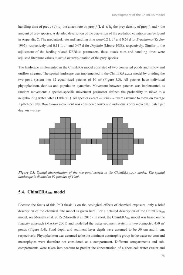
Development of the ChimERA model
75
handling time of prey j (d); ′ the attack rate on prey j (L d-1); the prey density of prey j; and n the
amount of prey species. A detailed description of the derivation of the predation equations can be found
in Appendix C. The used attack rate and handling time were 0.2 L d-1 and 0.76 d for Brachionus (Krylov
1992), respectively and 0.11 L d-1 and 0.07 d for Daphnia (Moore 1988), respectively. Similar to the
adjustment of the feeding-related DEBkiss parameters, these attack rates and handling times were
adjusted literature values to avoid overexploitation of the prey species.
The landscape implemented in the ChimERA model consisted of two connected ponds and inflow and
outflow streams. The spatial landscape was implemented in the ChimERAfoodweb model by dividing the
two pond system into 92 equal-sized patches of 10 m² (Figure 5.3). All patches have individual
phytoplankton, detritus and population dynamics. Movement between patches was implemented as
random movement: a species-specific movement parameter defined the probability to move to a
neighbouring water patch (Table 5.1). All species except Brachionus were assumed to move on average
1 patch per day. Brachionus movement was considered lower and individuals only moved 0.1 patch per
day, on average.
Figure 5.3: Spatial discretization of the two-pond system in the ChimERAfoodweb model. The spatial landscape is divided in 92 patches of 10m².
5.4. ChimERAfate model
Because the focus of this PhD thesis is on the ecological effects of chemical exposure, only a brief
description of the chemical fate model is given here. For a detailed description of the ChimERAfate
model, see Morselli et al. 2015 (Morselli et al. 2015). In short, the ChimERAfate model was based on the
fugacity approach (Mackay 2001) and modelled the water-sediment system in two connected 450 m²
ponds (Figure 5.4). Pond depth and sediment layer depth were assumed to be 50 cm and 1 cm,
respectively. Phytoplankton was assumed to be the dominant autotrophic group in the water column and
macrophytes were therefore not considered as a compartment. Different compartments and sub-
compartments were taken into account to predict the concentration of a chemical: water (water and

Chapter 5
76
suspended solids), sediment (pore water and sediment solids), dissolved organic carbon, particulate
organic carbon and phytoplankton. Spatial discretization was obtained by dividing the two pond system
in 20 slices and describing the one-dimensional water flow between these slices. A hydrological module
was used to compute water volumes (m3) and fluxes (m3 h−1) on an hourly basis in the slices. Slices
reflect areas with identical hydrodynamic properties but are not necessarily equal in area (Figure 5.4).
All calculations in the fate model were performed for each of these 20 slices.
Because the model was dynamic, time-varying environmental variables could be used as an input for
the model. Important environmental variables included the temperature, hydrodynamics and trophic
state of the system. Temperature is not constant throughout the year and varies significantly between
regions. The temperature influences partitioning constants and rates in the fate model e.g. the Henry law
constant and the dissolution rate of detritus. Trophic state refers to the nutrient conditions in the system
and is often described qualitatively as either oligotrophic, mesotrophic or eutrophic. The nutrient
conditions will determine the phytoplankton concentrations in the system. The hydrodynamics of the
systems describe the water flow. An often used measure for the water flow is the water residence time:
the time needed for all water in a location to be replaced. The model was also capable of using time-
varying chemical emissions as input to predict chemical concentrations in the different compartments at
different time points.
Figure 5.4: The spatial configuration in the ChimERAfate model. (A) Side view of the two connected ponds. Blue arrows indicate the direction of the water flow, red arrows represent the flow of the chemical. (B) Top-down view of the two connected ponds. Red dashed lines indicate the division of the system in 20 slices by the ChimERAfate model.

Development of the ChimERA model
77
The compartments included in the ChimERAfate model that were relevant for the ChimERAfoodweb model
were the phytoplankton, detritus and water concentration of the chemical. Phytoplankton and detritus
dynamics were described in the ChimERAfate model using ordinary differential equations (Equations 5.1
and 5.2). The phytoplankton and detritus concentrations determined the energy available for the
individuals in the food web. The food web model in turn provided the phytoplankton and detritus losses
due to consumption. The water concentration of the chemical was used to determine possible effects on
the food web.
Phytoplankton growth was not constant throughout the year and was described by
(5.1)
with the change in phytoplankton concentration over time (mg ww d-1 L-1); the phytoplankton
concentration (mg ww L-1); the time (days); the gross primary production (d-1); the fraction
of spend on respiration (-); the fraction of spend on excretion (-); the carrying capacity
(mg ww L-1); the mortality rate of phytoplankton (d-1) and the phytoplankton losses due to
grazing (mg ww L-1 d-1).
Detritus concentration was closely linked to the phytoplankton dynamics and was described by
(5.2)
with the change in detritus concentration over time (mg ww d-1 L-1); the phytoplankton
mortality rate (d-1); the phytoplankton concentration (mg ww L-1); the detritus dissolution rate
(d-1); the detritus concentration (mg ww L-1) and the detritus losses due to consumption by
detritus feeders (mg ww d-1 L-1).
Gpp and K were two parameters that are specific for a given situation and were chosen on a case by case
basis. Standard values were taken for the other phytoplankton and detritus model parameters (De
Laender et al. 2015): Resp = 0.1; Excr = 0.1; Mort = 0.2 d-1; Dis = 0.01 d-1.
5.5. Technical implementation
The main technical challenge was coupling the fate model and the food web model which differed
greatly in their architecture and internal communication. Instead of implementing direct communication
between the two models, the ChimERAfate model and the ChimERAfoodweb model were coupled by
coordinating the communication via a server (Figure 5.5). The advantage of this approach is that it is
very flexible i.e. different models can easily be plugged in, regardless of the encoding language since
only simple text strings with the necessary information are exchanged with the server. As long as they
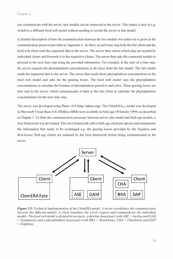
Chapter 5
78
can communicate with the server, new models can be connected to the server. This makes it easy to e.g.
switch to a different food web model without needing to recode the server or fate model.
A detailed description of how the communication between the two models was achieved is given in the
communication protocol provided in Appendix C. In short, at each time step both the fate client and the
food web client send the requested data to the server. The server then selects which data are needed by
individual clients and forwards it to the respective clients. The server then asks the connected models to
proceed to the next time step using the provided information. For example, at the start of a time step,
the server requests the phytoplankton concentrations in all slices from the fate model. The fate model
sends the requested data to the server. The server then sends these phytoplankton concentrations to the
food web model and asks for the grazing losses. The food web model uses the phytoplankton
concentrations to calculate the biomass of phytoplankton grazed in each slice. These grazing losses are
then sent to the server, which communicates it back to the fate client to calculate the phytoplankton
concentrations for the next time step.
The server was developed using Pharo v4.0 (http://pharo.org). The ChimERAfate model was developed
in Microsoft Visual Basic 6.0. DEBkiss IBMs were available in NetLogo (Wilensky 1999), as described
in Chapter 3. To limit the communication necessary between server, fate model and NetLogo models, a
Java framework was developed. This Java framework calls a NetLogo client per species and summarizes
the information that needs to be exchanged e.g. the grazing losses provided by the Daphnia and
Brachionus NetLogo clients are summed by the Java framework before being communicated to the
server.
Figure 5.5: Technical implementation of the ChimERA model. A server coordinates the communication between the different models. A client translates the server request and commands for the individual models. The food web model is divided in two parts, a detritus-based part (with ASE = Asellus and GAM = Gammarus) and a phytoplankton based part (with BRA = Brachionus, CHA = Chaoborus and DAP = Daphnia).

Development of the ChimERA model
79
Phytoplankton and detritus concentrations at the start of the year are too low to support the food web.
In reality, species have different strategies to overwinter. Therefore, we assumed that food web
dynamics only started when a critical food concentration of 0.025 mg ww L-1 was reached. Simulations
were started with 100 ind L-1. Early simulations showed that populations of Daphnia and Brachionus
can reach high densities (> 106 individuals in the whole system) which increased the simulation times
considerably. For the two grazers, a superindividual approach was therefore implemented to limit the
computation times. Following the kiss principle, an implementation with limited complexity was
chosen. Superindividuals were considered as one constant unit and were simulated in the same way as
normal individuals (Grimm and Railsback 2013). The only adjustment made was that the amount of
food eaten by the grazers was scaled to the superindividual level i.e. 100 individuals per superindividual
for Daphnia and 1000 individuals per superindividual for Brachionus. Although this approach limits the
variability in a population, it requires few additional assumptions and allows for an easy interpretation
of the simulations.
5.6. Applications
The ChimERA model developed here is an innovative method because it immediately links realistic
exposure predictions of chemicals to effects on food web dynamics. The flexibility and modularity of
the model make it possible to apply the ChimERA model to any environmental and ecological scenario.
Scenarios can differ, among others, in their spatial structure, identity of the emitted chemical, emission
strength and frequency, species in the food web and food web structure. Scenarios can be simulated by
supplying the currently used submodels with the necessary information or, if the currently implemented
submodels are insufficient, by plugging in a more suitable fate or food web model. To demonstrate its
potential, the use of the ChimERA model as a scenario analysis tool is explored in the next chapter. The
ChimERA model will be used to study how differences in the environmental variables of a scenario lead
to differences in the effects of the applied chemicals on food web dynamics.


81
6 THE CHIMERA MODEL AS A
SCENARIO ANALYSIS TOOL
Chapter 6
82
Abstract
The integrated ChimERA model was developed as a tool to perform more realistic ecological risk
assessments. To test its performance, the ChimERA model was applied to a two-pond system connected
by a stream in which 15 hypothetical scenarios – differing in water residence time, temperature, trophic
state and applied chemical (carbendazim, chlorpyrifos, pyrene and the mixture of the three chemicals)
– were evaluated. The predicted effects of the applied chemicals were clearly different for the selected
scenarios. Densities of species were generally highest in scenarios with a high trophic state temperature
and water residence time. Daphnids were the dominant grazers in the ponds while rotifers dominated
in the streams. Concentrations of applied chemicals were highest in scenarios with a high water
residence time. The physico-chemical properties of the chemical determined the spatial and temporal
pattern of the exposure i.e. where the concentrations were highest and how fast the chemical
disappeared. As expected from their sensitivities to the chemicals, direct effects were predicted on
Chaoborus, Daphnia and Gammarus. These effects were, however, heterogeneously distributed in space
and time and reflected the predicted differences in exposure. The most notable indirect effects were
shifts in dominance from Daphnia and Gammarus to Brachionus and Asellus, respectively. Also, the
predator Chaoborus was affected indirectly through effects on its prey species Daphnia. For the mixture
of three chemicals, the effects of pyrene dominated for Daphnia and the effects of carbendazim and
chlorpyrifos for Gammarus. These simulations demonstrate how much the outcome of chemical
exposure is determined by environmental conditions, which cannot be captured with traditional risk
assessment methods. Modelling tools like the ChimERA model can prove essential to answer the current
challenges of ecological risk assessments.

The ChimERA model as a model analysis tool
83
6.1. Introduction
The ChimERA model was developed (Chapter 5) to demonstrate (proof of principle) how available
knowledge and models can be combined into a predictive risk assessment tool applicable in a range of
environmental conditions (De Laender et al. 2014a). To evaluate and demonstrate how such a type of
model could be used to perform scenario analysis, the ChimERA model was applied to 15 hypothetical
scenarios that differed in their environmental conditions and applied chemical(s). Although the main
focus of this chapter is on the ecology and food web dynamics, a short discussion of the chemical fate
model is also included.
6.2. Methods
6.2.1. Scenario description
Three environmental variables can be manipulated in the ChimERA model: temperature, trophic state
and hydrodynamics. Trophic state refers to the amount of nutrients available in the system: oligotrophic,
mesotrophic or eutrophic. Hydrodynamics refer to how fast the water flows and thus the retention time
of the water in the ponds. As numerous combinations of these environmental variables and thus
environmental scenarios are possible, we selected three different ‘example’ combinations of these
variable to evaluate the potential applications and limitations of the ChimERA model (Table 6.1):
Scenario I is a high velocity system with a low average annual temperature and an oligotrophic nutrient
status. Scenario II is characterized by intermediate water velocity, medium average annual temperature
and a mesotrophic nutrient status. Scenario III has a low water velocity, high average annual temperature
and eutrophic nutrient conditions.
Table 6.1: Description of the selected scenarios. Scenarios differ in their temperature, trophic state and hydrodynamics. Annual minimum and maximum temperatures are shown. K = phytoplankton carrying capacity; Gpp = gross primary production; RT = residence time.
Scenario Temperature (Di Guardo et al.)
Trophic State (Håkanson and Peters 1995)
Hydrodynamics (Peretyatko et al. 2007)
I [4.2 - 20.1] °C K = 0.3 mg ww L-1; Gpp = 0.36 d-1
RT = 5 d
II [4.3 - 22.0] °C K = 0.5 mg ww L-1: Gpp = 0.42 d-1
RT = 25 d
III [6.9 - 26.3] °C K = 1 mg ww L-1: Gpp = 0.71 d-1
RT = 100 d
Chapter 6
84
These three selected environmental scenarios were combined with five exposure scenarios: no exposure,
exposure to carbendazim, exposure to chlorpyrifos, exposure to pyrene and finally exposure to all three
chemicals simultaneously. The three selected chemicals differ greatly in their physico-chemical
properties and their exposure pattern (Appendix D: Table D1). Carbendazim is a fungicide used to
control plant diseases (van Wijngaarden et al. 1998) and chlopyrifos is a widely-used insecticide (van
der Hoeven and Gerritsen 1997). Pyrene is a polycyclic aromatic hydrocarbon (PAH) that is mostly
formed as a by-product of anthropogenic activities (e.g. fossil fuel combustion). Pyrene mainly enters
the aquatic environment accidentally through e.g. petroleum spills, wastewater or surface run-off
(Nikkilä et al. 1999). Actual emission rates for these chemicals are difficult to find and are highly site-
specific. The current study is a proof of principle assessment and the performance of the ChimERA
model can best be discussed when effects are expected to occur. Therefore, emission strengths were
chosen to result in maximum water concentrations close to the acute LC50-values of the most sensitive
species in the intermediate scenario II (Appendix D: Table D2). Both pesticides were considered to have
a highly seasonal emission pattern, with short application periods in spring (day 180) and late summer
(day 260; Figure 6.1). The length of the application periods was ten days: emission concentrations
increased during the first five days and then decreased again. Maximum emission strengths were 3.7 ∙
10-4 mol L-1 h-1 and 6.7 ∙ 10-7 mol L-1 h-1 for carbendazim and chlorpyrifos, respectively. Pyrene was
considered to have a continuous ambient exposure pattern, with stable emission concentrations of 2 ∙ 10-
6 mol L-1 h-1 throughout the year (Figure 6.1).
The five species in the food web (Chapter 5) differed in their sensitivity to these three chemicals
(Appendix D: Table D2). Gammarus and Daphnia were most sensitive to carbendazim: the acute LC50
was 55 μg L-1 and 91 μg L-1, respectively (van Wijngaarden et al. 1998). No effects on Chaoborus were
observed in toxicity tests at concentration of up to 3435 μg L-1 (van Wijngaarden et al. 1998). For
chlorpyrifos, Gammarus, Chaoborus and Daphnia were considered the only sensitive species: the acute
LC50 was 0.23 μg L-1, 0.3 μg L-1 and 0.8 μg L-1, respectively. Gammarus and Daphna were also the most
sensitive of the five species when exposed to pyrene: the acute LC50 was 27.1 μg L-1 and 68 μg L-1,
respectively (Chapter 2). No pyrene effects were observed at nominal concentrations of up to 2000 μg
L-1 for Brachionus and Chaoborus (Chapter 2). Brachionus toxicity test results were not available for
carbendazim and chlorpyrifos but rotifers are often more tolerant to chemicals than cladocerans (Girling
et al. 2000) and no effects of these chemicals on rotifers were therefore assumed at the used exposure
concentrations.
Because mortality and organism mobility in the DEBkiss IBMs are stochastic processes, variability is
expected between simulations. To account for this variability, simulations are typically iterated multiple
times. However, in this case, simulation times for one scenario were as high as 3 hours, limiting the
number of iterations possible. As a compromise, each scenario was run five times. Ideally, model
performance is assessed by comparing model simulation with observations. However, these

The ChimERA model as a model analysis tool
85
observations were not available for the system and exposure scenarios modelled here. As an alternative
approach, the scenario expectations were defined based on a priori knowledge and compared with the
simulations. The expected environmental fate of each chemical was defined based on the physico-
chemical characteristics,. For the food web, the interactions between species and the sensitivity of each
species to the chemical were taken into account to define a priori expected population dynamics.
Figure 6.1: Used emission patterns for (A) carbendazim, (B) chlorpyrifos and (C) pyrene.
6.2.2. Expectations regarding the outcome of the scenario analyses
6.2.2.1. ChimERAfate
In this section, a short description is given for each chemical of how their physico-chemical properties
(Appendix D: Table D1) influence their environmental fate and how this is altered by changes in
temperature, trophic state and water retention time. At the end of this section, a summary is given of the
expectations for each chemical per scenario.

Chapter 6
86
Carbendazim is a hydrophilic substance (logKow = 1.52) and will thus not accumulate in the sediment.
Moreover, degradation is slow (HLwater = 720 h). Carbendazim will thus mainly disappear from the
system with the water outflow and, because of the low sediment accumulation, the short peaks in
emission are expected to be reflected by short peaks in water concentrations. The water retention time
will thus be an important factor for its environmental fate. Chemical concentrations will be higher in
systems with high water retention time: for the same amount of chemical emitted over an hour, the
chemical is diluted less when the water is flowing slowly. Carbendazim will thus be present in the water
longer and in higher concentrations in systems with high water residence times. Because of the limited
sediment accumulation and degradation, carbendazim concentrations are not expected to be influenced
much by temperature or the trophic state of the system, which mainly influence degradation and
accumulation.
Chlorpyrifos is a more hydrophobic substance (logKow = 4.96) and degrades quickly (HLwater = 24 h).
Accumulation in the sediment and degradation are thus important environmental processes for this
chemical. As a result of the high sediment accumulation, a long period of reduced but constant water
concentrations are expected after a peak in emission. More organic material is available in eutrophic
systems compared to oligotrophic systems, which leads to, among others, more accumulation in the
sediment. Temperature increases the phytoplankton growth and biomass, further increasing the amount
of organic material available in the system. Also, the temperature positively influences the degradation
rate of the chemical. Temperature and trophic state will thus determine the water concentrations together
with the water retention time. As described for carbendazim, higher water concentrations are expected
for systems with high water retention time. However, high water retention times also increase the time
available for accumulation to the sediment and for degradation, both decreasing the water concentration
of the chemical. Which process is dominant is hard to predict a priori because this depends on the
relative strength of the environmental fate processes.
Pyrene is a hydrophobic substance (logKow = 5.18) that degrades slowly (HLwater = 17 ∙ 103 h). Pyrene
will thus accumulate in the sediment and persist. Because of the continuous emission pattern, constant
water concentrations are expected once equilibrium between all environmental compartments is
reached. As was the case for chlorpyrifos, temperature and trophic state are expected to increase the
accumulation in the system, decreasing the water concentrations of pyrene. The effect of water retention
time is more predictable than for chlorpyrifos: a high water retention time will increase the water
concentrations because of the lower dilution of the chemical. Effects of the water retention time on
accumulation and degradation are negligible because of the continuous emission of pyrene.
In summary, for the three selected environmental scenarios, carbendazim concentrations in scenario III
are expected to be higher than in scenario II and I because of the longer residence times (100 days versus
25 and 5 days, respectively; Table 6.1). Peaks in carbendazim concentration are expected to disappear

The ChimERA model as a model analysis tool
87
quickly in all scenarios because of the limited accumulation, with the narrowest peak in scenario I. For
chlorpyrifos and pyrene, it is harder to predict a priori how the concentrations will differ between the
scenarios. Water concentrations are expected to decrease with temperature and trophic state but the
opposite is expected for water retention time. The differences between scenario I, II and III will thus
reflect the relative importance of these three environmental variables. Chlorpyrifos peaks are expected
to persist longer in scenario III than in scenario II and I because of the longer residence time and, as a
result of the higher temperature and trophic state, the increased accumulation in the sediment. As was
the case for chlorpyrifos, differences in pyrene concentrations between the three scenarios are hard to
predict. Pyrene concentrations are expected to become constant once equilibrium between the
compartments has been reached.
6.2.2.2. ChimERAfoodweb
This section starts with a description of how the food web dynamics are expected to be influenced by
the environmental conditions. Next, the expected effects of the applied chemical(s) on the food web
dynamics are discussed. Finally, a summary of the expected outcomes of the scenarios is given.
The phytoplankton carrying capacity and gross primary production, indicators for the trophic state in
the fate model, will determine the phytoplankton biomass and growth. A higher phytoplankton biomass
means more energy is available for the grazers. The densities of the grazers Daphnia and Brachionus
and their predator Chaoborus are thus expected to be higher when the trophic state of the system is high.
Phytoplankton is the main source for detritus and detritus dynamics are thus closely linked to the
phytoplankton dynamics. In the absence of phytoplankton grazing, a high trophic state is expected to
lead to high detritus concentrations, which allows the densities of the detritus feeders Asellus and
Gammarus to be higher. Phytoplankton grazing will limit the biomass of phytoplankton being converted
to detritus, making it harder to predict how the detritus concentrations will differ between trophic states.
Because of the close link between phytoplankton and detritus, patterns in the phytoplankton dynamics
are expected to be reflected in the detritus dynamics. Because of the strong relation between their food
sources, patterns in grazers and detritus feeders are also expected to be linked. Chaoborus dynamics in
turn are expected to reflect the dynamics of its food source, the grazers. Phytoplankton drift with the
water is not considered in the fate model and the water retention time thus should not influence the food
web dynamics.
Gammarus and Daphnia are the most sensitive species to the three chemicals considered here. Exposure
to these three chemicals is therefore expected to lead to decreased abundances of Gammarus and
Daphnia. Direct effects of chlorpyrifos are also expected for Chaoborus but not for the other two
chemicals. As indirect effects, the densities of the more tolerant competitors Asellus and Brachionus are
expected to increase. Chaoborus feeds on both Daphnia and Brachionus and because both prey species
Chapter 6
88
are differently affected by carbendazim and pyrene, it is difficult to predict how these two chemicals
will affect the predator dynamics. In the case of chlorpyrifos, direct effects are expected for both
Chaoborus and Daphnia. Indirect effects on Brachionus are thus expected to be especially strong
because of both reduced competition and predation by chlorpyrifos. Since chlorpyrifos and carbendazim
are applied only during short periods, (partial) recovery of the Gammarus and Daphnia densities should
be possible after the application periods. Pyrene exposure is constant throughout the year and
consistently different food web dynamics from the control scenarios are therefore expected. When
exposed to the mixture of all three chemicals, the continuous exposure to pyrene is expected to affect
the food web the most because the exposure starts earlier: Daphnia and Gammarus densities will
decrease and indirect effects on Asellus, Brachionus and Chaoborus will occur. The application of the
other two chemicals will further increase the effects of pyrene, leading to higher effects than observed
in the individual exposures.
In summary, the densities of all species in the food web are expected to be higher in scenario III than in
scenario II and I because of the higher trophic state and temperature in that scenario. Direct effects of
the chemicals are mainly expected for Daphnia and Gammarus while Asellus, Brachionus and
Chaoborus will be indirectly affected through reduced competition or reduced prey availability. The
magnitude of the predicted effects of the chemicals on the food web is closely linked to the expected
exposure patterns (See 6.2.2.1). For carbendazim, higher concentrations are expected in scenario III than
in scenario II and I, and higher effects on the food web dynamics are thus also expected. For chlorpyrifos
and pyrene, the expected concentration differences between the scenarios are less clear and it is thus
hard to predict differences in effects between the scenarios.
6.3. Results
For a clear presentation of the simulations, four slices (see 5.4) were chosen that were representative for
the whole system (Figure 6.2): slice 1 was located at the inflow of the first pond i.e. where the chemicals
were emitted into the system, slice 5 was located in the middle of the first pond, slice 10 was located in
the stream between the first and second pond and slice 15 was located in the middle of the second pond.
The observed patterns in the simulations are described in this section for the ChimERAfate (6.3.1) and
ChimERAfoodweb (6.3.2) model and compared to the expected patterns. The evaluation of the underlying
processes is described in section 6.4.

The ChimERA model as a model analysis tool
89
Figure 6.2: Location of slices 1, 5, 10 and 15, for which the population dynamics are shown in Figures 6.3-6.13.
6.3.1. ChimERAfate
In this section, the expected results of the ChimERAfate model are compared with the performed
simulations for each chemical. The dominant fate processes for each chemical are also provided. For a
discussion of the observed patterns and the underlying processes, see 6.4.1.
As expected because of the higher water residence time, carbendazim concentrations in slice 1 were
higher in scenario III (971.87 μg L-1) than in scenario II (255.54 μg L-1) and scenario I (51.92 μg L-1).
Because of the increased water retention time, the decrease in carbendazim concentrations throughout
the two-pond system was also higher in scenario III than in scenario II and scenario I (Figure 6.3): the
carbendazim concentration in the outflow stream (slice 20) was 50.9%, 11.1% and 2.5% of the
concentration in the inflow stream (slice 1) for scenario I, II and III, respectively. Because of the limited
sediment accumulation, concentrations of carbendazim are expected to decrease sharply when emission
stops. This was indeed observed for scenario I and scenario II but not for scenario III. In scenario III,
the carbendazim concentration only decreased sharply after emission in slice 1, where emission
occurred. Further downstream, peaks were much less pronounced (slice 5) or not observed (slice 15).
Outflow with water, diffusion to sediment pore water and degradation were the most important fate
processes for carbendazim.
Chlorpyrifos concentrations were higher in scenario III (1.55 μg L-1) than in scenario II (0.42 μg L-1)
and I (0.09 μg L-1), indicating that water retention time was more important than temperature and trophic
state (see 6.2.2.1). As expected, a reduced but constant chlorpyrifos concentration was predicted after
the application period because of the accumulation in the sediment (Figure 6.3). The peak chlorpyrifos
concentrations decreased sharply further downstream and this was more pronounced with higher water
residence times: peak chlorpyrifos concentrations in slice 20 were 21.8%, 0.3% and <0.01% of the peak

Chapter 6
90
concentrations in slice 1 for scenario I, II and III, respectively. Outflow with water and degradation were
the most important processes that determined the chlorpyrifos water concentration.
Pyrene concentrations were higher for scenario III (6.79 μg L-1) than in scenario II (1.73 μg L-1) and
scenario I (0.35 μg L-1) and, as expected, concentrations stayed constant once equilibrium was reached
(Figure 6.3). This equilibrium between all environmental compartments was reached later further away
from the emission source. Pyrene concentrations decreased further downstream and this was more
pronounced in scenarios with a high water retention time: pyrene concentrations in the outflow stream
were 87.0%, 52.5% and 9.9% of the concentrations in the inflow stream for scenario I, II and III,
respectively. For pyrene, the dominating fate processes were the outflow with water and the particle
deposition to the sediment.
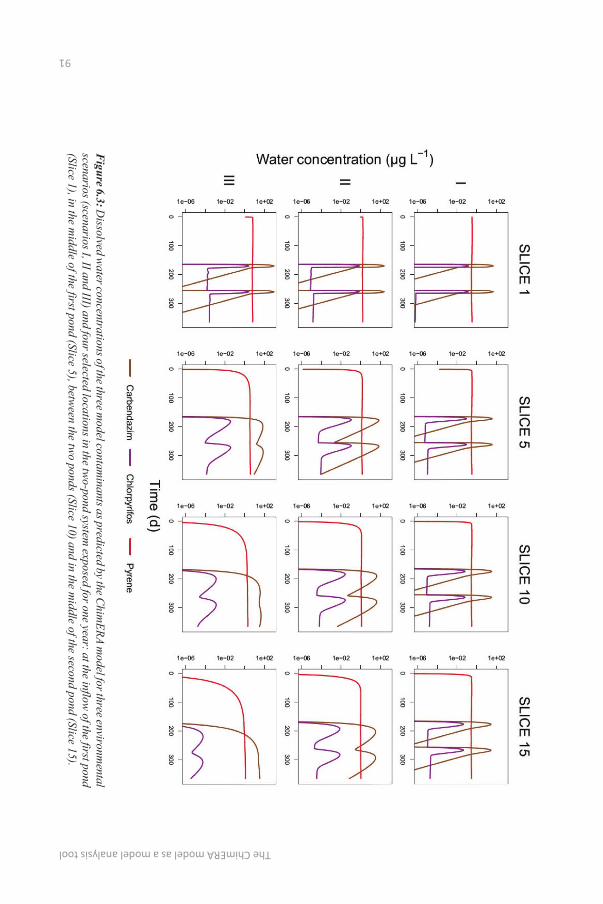
The ChimERA model as a model analysis tool
91
Figure 6.3: D
issolved water concentrations of the three m
odel contaminants as predicted by the C
himERA m
odel for three environmental
scenarios (scenarios I, II and III) and four selected locations in th e two-pond system
exposed for one year: at the inflow of the first pond
(Slice 1), in the middle of the first pond (Slice 5), betw
een the two ponds (Slice 10) and in the m
iddle of the second pond (Slice 15).
() lll a-<1> g_ lll t:!. 3
() :::r 0
~ 5 "'
"1J '< (i) :::1 <1>
Water con centration (1-19 L -1)
1e-o6
8
8
8
1e-o6
8
8
8
-i 3" (!) 1e-06 -a. 0
8
8
8
1e-o6
1e-Q2
1e-Q2
1e-Q2
1e-Q2
,F\
1e+02
1e+02
1e+02
1e+02 1
8~
!H ) I I
1e-ll6 1e-Q2 10+02
8
:~ 1e-ll6 1e-Q2 1e+02
8
8
8
1e-ll6 1e-Q2 1e+02
8
8
8
1e-ll6 1e-Q2 1e+02
I : l I
· ~ I
I 8 ~ ~ î)
I !H / I )
1e-ll6 1e-Q2 1e+02
8
:b 1e-ll6 1e-Q2 1e+02
8
8
8
1e-ll6 1e-Q2 1e+02
8
8
8
1e-ll6 1e-Q2 1e+02 I I I I
I : l l I 8 ~ r:::::;:-r
I 8 I - ~
tQ r 0 m --"
tQ r 0 m (.Tl
tQ r () m --" 0
ltQ c
I~ --"
I (.Tl
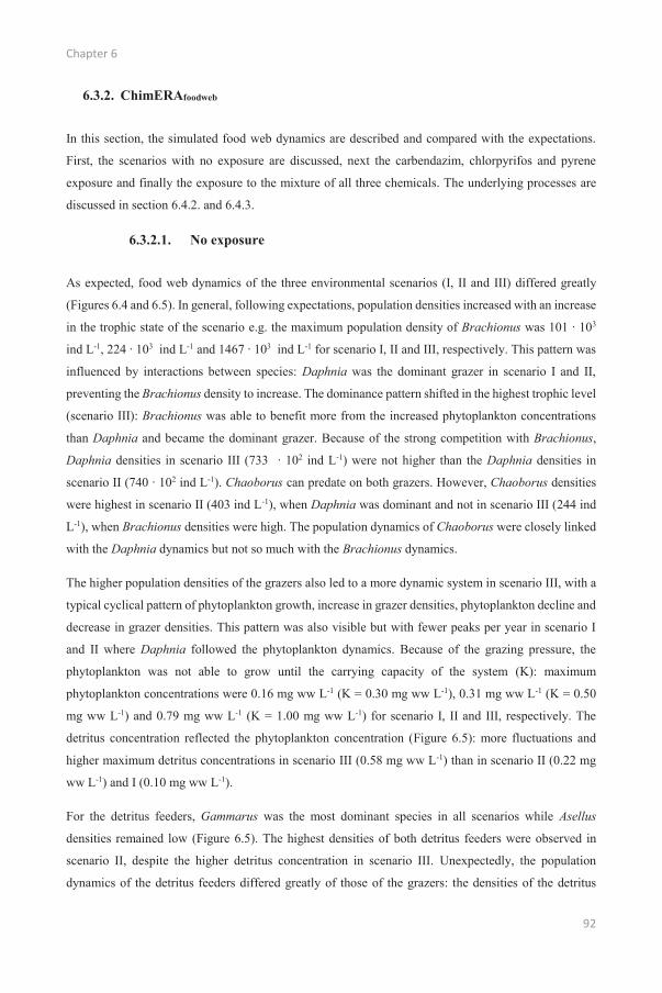
Chapter 6
92
6.3.2. ChimERAfoodweb
In this section, the simulated food web dynamics are described and compared with the expectations.
First, the scenarios with no exposure are discussed, next the carbendazim, chlorpyrifos and pyrene
exposure and finally the exposure to the mixture of all three chemicals. The underlying processes are
discussed in section 6.4.2. and 6.4.3.
6.3.2.1. No exposure
As expected, food web dynamics of the three environmental scenarios (I, II and III) differed greatly
(Figures 6.4 and 6.5). In general, following expectations, population densities increased with an increase
in the trophic state of the scenario e.g. the maximum population density of Brachionus was 101 ∙ 103
ind L-1, 224 ∙ 103 ind L-1 and 1467 ∙ 103 ind L-1 for scenario I, II and III, respectively. This pattern was
influenced by interactions between species: Daphnia was the dominant grazer in scenario I and II,
preventing the Brachionus density to increase. The dominance pattern shifted in the highest trophic level
(scenario III): Brachionus was able to benefit more from the increased phytoplankton concentrations
than Daphnia and became the dominant grazer. Because of the strong competition with Brachionus,
Daphnia densities in scenario III (733 ∙ 102 ind L-1) were not higher than the Daphnia densities in
scenario II (740 ∙ 102 ind L-1). Chaoborus can predate on both grazers. However, Chaoborus densities
were highest in scenario II (403 ind L-1), when Daphnia was dominant and not in scenario III (244 ind
L-1), when Brachionus densities were high. The population dynamics of Chaoborus were closely linked
with the Daphnia dynamics but not so much with the Brachionus dynamics.
The higher population densities of the grazers also led to a more dynamic system in scenario III, with a
typical cyclical pattern of phytoplankton growth, increase in grazer densities, phytoplankton decline and
decrease in grazer densities. This pattern was also visible but with fewer peaks per year in scenario I
and II where Daphnia followed the phytoplankton dynamics. Because of the grazing pressure, the
phytoplankton was not able to grow until the carrying capacity of the system (K): maximum
phytoplankton concentrations were 0.16 mg ww L-1 (K = 0.30 mg ww L-1), 0.31 mg ww L-1 (K = 0.50
mg ww L-1) and 0.79 mg ww L-1 (K = 1.00 mg ww L-1) for scenario I, II and III, respectively. The
detritus concentration reflected the phytoplankton concentration (Figure 6.5): more fluctuations and
higher maximum detritus concentrations in scenario III (0.58 mg ww L-1) than in scenario II (0.22 mg
ww L-1) and I (0.10 mg ww L-1).
For the detritus feeders, Gammarus was the most dominant species in all scenarios while Asellus
densities remained low (Figure 6.5). The highest densities of both detritus feeders were observed in
scenario II, despite the higher detritus concentration in scenario III. Unexpectedly, the population
dynamics of the detritus feeders differed greatly of those of the grazers: the densities of the detritus

The ChimERA model as a model analysis tool
93
feeders mainly increased in the second half of the year while periods of population growth were observed
for grazers throughout the year.
Unexpectedly, clear spatial differences were observed between the species: population densities of
Daphnia and Chaoborus were much higher in the ponds (Slice 5 and 15) than in the inflow and
connecting streams (Slice 1 and 10). Based on the Brachionus dynamics in scenario III, spatial
differences are much less prominent for this species. Similar to Daphnia and Chaoborus, Asellus and
Gammarus population densities were highest in the ponds and lower in the inflow and connecting
streams. Contrary to the ponds, the reduced competition with Gammarus in the streams allowed short
periods of population increase for Asellus e.g. slice 1 and 15 in scenario I around day 230.
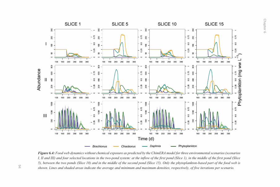
Chapter 6
94
Figure 6.4: Food web dynamics without chemical exposure as predicted by the ChimERA model for three environmental scenarios (scenarios I, II and III) and four selected locations in the two-pond system: at the inflow of the first pond (Slice 1), in the middle of the first pond (Slice 5), between the two ponds (Slice 10) and in the middle of the second pond (Slice 15). Only the phytoplankton-based part of the food web is shown. Lines and shaded areas indicate the average and minimum and maximum densities, respectively, of five iterations per scenario.
Q) (.) c ro "0 11 c :::J .0 <(
111
SLICE 1 SLICE 5 ~ ~ ~
~ ~ r ~ ~
;j I ~ I
[ ~ ; 100 150 200 250 300 350 100 150 200 250 300 350
lil ~ lil
i ~ ~ ~
~ "' 8 0 V
~ f\/\f'\.._ lQ 0
. 0 0 N
100 150 200 250 300 350 100 150 200 250 300 350
~ - ~ i!?
~ 0 § ~ ~
ci
~ lQ ~ ci
h h i/'1.... H · 71 Î
100 150 200 250 300 350 100 150 200 250 300 350
SLICE10 SLICE15 ~ ~ 0
~ :!l
~ ~
!; ~ !; !Q ~ ..., 0
d ~ ó ~ ~
ci
~ ~ ~
"' "' 0 lil 0 lil :;l
0 0 o o I ~~ " ~ ol ~=;=-...,_. ....J 100 150 200 250 300 350
~ lil ~ lil
~ g ~ g "' 8 0 V "' 8 0 V
lQ 0 . 0
0 N f'l1'h_ lQ 0 . 0
0 N
100 150 200 250 300 350
~ : ~~~~~~ ~ : 100 150 200 250 300 350
Time (d)
I I
100 150 200 250 300 350
~ ~ ~ Cl ::; E ._ ci c
0 !Q ~ ci c
~V :-=-'f ' )- f- 0 ~ 0
100 150 200 250 300 350
(\ ~
lik... -J·
100 150 200 250 300 350
>-~ ..c
i!? 0
~
ci
lQ ci
a..
-- Brachionus -- Chaoborus -- Daphnia - Phytoplankton
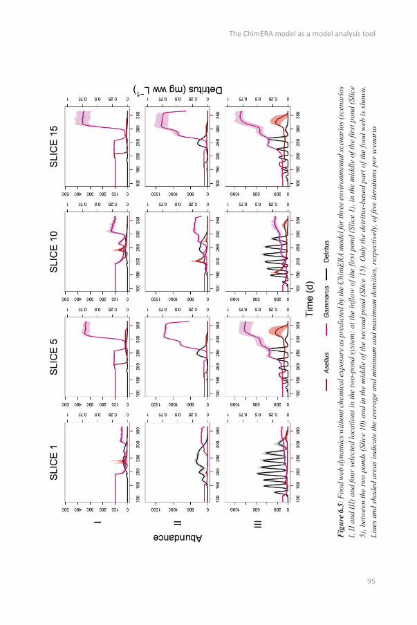
The ChimERA model as a model analysis tool
95
Fig
ure 6
.5: F
ood
web
dyn
amic
s with
out c
hem
ical
expo
sure
as p
redi
cted
by t
he C
him
ERA
mod
el fo
r thr
ee en
viro
nmen
tal s
cena
rios (
scen
ario
s I,
II a
nd II
I) a
nd fo
ur se
lect
ed lo
catio
ns in
the
two-
pond
syst
em: a
t the
inflo
w o
f the
firs
t pon
d (S
lice
1), i
n th
e m
iddl
e of
the
first
pon
d (S
lice
5), b
etw
een
the
two
pond
s (Sl
ice
10) a
nd in
the
mid
dle
of th
e se
cond
pon
d (S
lice
15).
Onl
y th
e de
tritu
s-ba
sed
part
of t
he fo
od w
eb is
show
n.
Line
s and
shad
ed a
reas
indi
cate
the
aver
age
and
min
imum
and
max
imum
den
sitie
s, re
spec
tivel
y, o
f fiv
e ite
ratio
ns p
er sc
enar
io
( ~_l MM 5w) snl!Jlaa SL'O s·o sz·o I SL'O S'O sz·o 0 SL'O S'O SZ'O
~ ~ ~ I{) ~ ~ ~ ..--w ~ ~ ~ ü ::i ~ ~ ~ (/)
~ ~ ~
§ § §
oos oo• ooc ooz OOI 0 ooa 0001 oos 0001 009 ooz 0
SL'O s·o sz·o SL'O s·o sz·o SL'O s·o sz·o
~ ~ ~
0 ~ ~ ~ ..--"' w ~ ~ ~ a
ü -~
_J ~ ~ ~ D
(/) ~ ~ ~ -§ ê § ~ "' 2
oos oo• ooc ooz OOI 0 OOSI 0001 oos 0001 009 ooz 0 Q) "' E E SL'O s·o sz·o SL'O s·o sz·o SL'O s·o sz·o E
F "' (!)
~ ~ ~
I{) ~ ~ ~ w ~ ~ ~ "' ü :;,
== ::i ~ ~ ~ Q)
"' (/) <(
~ ~ ~
§ ê ê oos oo• ooc ooz OOI 0 OOSI 0001 oos 000~ 009 ooz 0
SL'O s·o sz·o SL'O s·o sz·o SL'O s·o sz·o
~ ~ ~
..-- ~ ~ ~ w ~ ~ ~ ü ::i ~ ~ ~ (/)
~ ~ ~
§ ê § oos oo• ooc ooz OOI 0 OOSI 0001 oos oom 009 ooz 0
a~uepunqv

Chapter 6
96
6.3.2.2. Carbendazim exposure
Direct effects
As a result of the low carbendazim concentrations, only minimal effects of carbendazim on the food
web dynamics were observed in scenario I (Figure 6.6-6.7). In scenario II and III, the expected negative
effects of carbendazim exposure to Daphnia and Gammarus densities were observed. High spatial
differences between the direct effects of carbendazim on Daphnia densities were observed in scenario
II and III: carbendazim effects were mainly observed in the first pond and were lower and occurred later
in the year in the second pond (slice 15), reflecting the lower carbendazim concentrations downstream.
As a result of the higher carbendazim concentrations, effects were more pronounced in scenario III than
in scenario II: after the first carbendazim application, the Daphnia densities decreased by 56% in the
first pond (slice 5) in scenario II while, in scenario III, Daphnia went extinct in the first pond (Figure
6.6). Recovery was only observed in the first pond in scenario II, where Daphnia densities increased
again after the first exposure peak (around day 250). The reached densities after recovery were, however,
only about 40% of the densities in the control scenario and the population peak occurred later (day 250
instead of day 200).
Carbendazim effects on Gammarus densities were observed in the whole system for both scenario II
and III (Figure 6.7): the strong population growth phase at the end of the year, observed in the control
scenarios (Figure 6.5), was no longer observed. Similar to the carbendazim effects on Daphnia, the
effects of carbendazim were lower and occurred later in the second pond, especially in scenario III.
Indirect effects
Because direct effects of carbendazim were nearly absent in scenario I, indirect effects were mainly
observed in scenario II and III on Asellus, Brachionus and Chaoborus. Indirect effects of carbendazim
were especially visible for the detritus feeders (Figure 6.7): the tolerant Asellus was able to become the
dominant species throughout in the system in both scenarios e.g. an increase in density by 329% in
scenario II. Reflecting the direct effects of carbendazim on Gammarus, the indirect effects occurred later
and the Asellus densities were lower in the second pond than in the first pond.
For the grazers, in scenario II, the densities of the more tolerant Brachionus were higher after
carbendazim exposure, although no shift in dominance occurred (Figure 6.6). As was the case for the
direct effects, spatial differences were observed: Brachionus initially increased in density in the first
pond after the first carbendazim application (day 160) but decreased again once Daphnia densities
recovered. In the second pond, carbendazim effects were nearly absent after the first carbendazim
application but an increase in Brachionus density was observed after the second application (day 250).
In scenario III, these spatial differences were even more pronounced. In the first pond, the carbendazim

The ChimERA model as a model analysis tool
97
application further increased the dominance of Brachionus leading to an increase in the number of peaks
in Brachionus density (from 5 to 7). In the second pond, however, indirect effects were absent.
Because Chaoborus can feed on both grazers, it was hard to formulate expectations for the indirect
effects of carbendazim. Apparently, the predator Chaoborus was affected indirectly in scenarios II and
III through the effects of carbendazim on the prey species Daphnia (Figure 6.6). As was the case for
Daphnia, effects were most pronounced in the first pond. In scenario II, Chaoborus densities decreased
by 32% in slice 5 but, following the recovery of Daphnia, stayed high for a longer period. In the second
pond, indirect effects were only observed at the end of the year by the absence of a second population
peak. In scenario III, Chaoborus followed the extinction of Daphnia in the first pond but no indirect
effects were observed in the second pond.
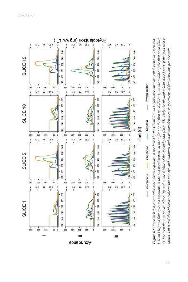
Chapter 6
98
Fig
ure
6.6:
Foo
d w
eb d
ynam
ics w
ith ca
rben
dazi
m e
xpos
ure a
s pre
dict
ed b
y the
Chi
mER
A m
odel
for t
hree
env
iron
men
tal s
cena
rios
(sce
nari
os
I, II
and
III)
and
four
sele
cted
loca
tions
in th
e tw
o-po
nd s
yste
m: a
t the
inflo
w o
f the
firs
t pon
d (S
lice
1), i
n th
e m
iddl
e of
the
first
pon
d (S
lice
5), b
etwe
en th
e tw
o po
nds
(Slic
e 10
) and
in th
e m
iddl
e of
the
seco
nd p
ond
(Slic
e 15
). O
nly
the
phyt
opla
nkto
n-ba
sed
part
of th
e fo
od w
eb is
sh
own.
Lin
es a
nd sh
aded
are
as in
dica
te th
e av
erag
e an
d m
inim
um a
nd m
axim
um d
ensi
ties,
resp
ectiv
ely,
of f
ive
itera
tions
per
scen
ario
.
( ~-1 MM 6W) UOptUeidOlÁ4d SL'O S'O SZ'O 0 I SL'O S'O Sl'O 0 I SL'O S'O SZ'O
~ ~ I{) ~ ..-- ~ ~
w ~ ü ::i ~ (/)
~
~
c
~
~
~
§ ~ ê c: osc osz OSI os 0 009 009 oo• ooz OOS I 0001 005 .9
"' c: SL'O s·o SZ'O SL'O s·o Sl'O SL'O s·o sz·o "' ä.
~
0 ~ ..--
~
~ j 0
~ >. .t::. a.
~
w ~ ü __J ~ (/)
~
§
~
~
~ ~
ê
~
~ .!,!!
~ c: .c: - g. § ~ 0
osc osz OSI os 0 009 009 oo• ooz OOSI 0001 005 Q)
SL'O s·o SZ'O SL'O s·o sc:·o SL'O s·o sz·o E F
~
I{) ~ w ~ ü
~
~
~
~ ., ;::
~ 2 0
"' ~ .c: ü
::i ~ (/)
~ ~
~ ~ ~
§ osc osz OSI os 0 008 009 oo• ooz
ê OOSI 0001 005
ê ~ c: .Q '5
SL'O s·o SZ'O SL'O s·o sc:·o SL'O s·o sz·o ~ IXl
~ ~ ~
..-- ~ ~ ~ w ~ ü ~ ~
::i ~ (/) ~ ~
~ ~ ~
§ ê § osc osz OSI os 0 008 009 oo• ooz OOSI 0001 005
a~uepunqv

The ChimERA model as a model analysis tool
99
Figure 6.7: Food w
eb dynamics w
ith carbendazim exposure as predicted by the C
himERA m
odel for three environmental scenarios (scenarios
I, II and III) and four selected locati ons in the two-pond system
: at the inflow of the first pond (Slice 1), in the m
iddle of the first pond (Slice 5), betw
een the two ponds (Slice 10) and in the m
iddle of the second pond (Slice 15). Only the detritus -based part of the food web is show
n. Lines and shaded areas indicate the average and m
inimum
and maxim
um densities, respectively, of five iterations per scenario.
Abundance
- - -0 200 600 1000 0 500 1500 2500 0 100 200 300 400 500
8 8 8
~ ~ ~
8 8 8
~ (/) r
~ ~ ~ 0 m
8 8 8 ......
~ ~ ~
0.25 0.5 0.75 1 0 0.25 0.5 0.75 1 0 0.25 0.5 0.75
0 200 600 1000 0 500 1500 2500 0 100 200 300 400 500
8 8 8
~ ~ ~ ):.
8 8 8
h (/)
"' r tb ê'
~ ~ ~ 0
"' m 8 8 8 CJ1
~ ~ ~ G) -i Q)
~ï 0 0.25 0.5 0.75 1 0 0.25 0.5 0.75 1 0 0.25 0.5 0.75
3 3 ct> 0 200 600 1000 0 500 1500 2500 0 100 200 300 400 500 Q)
2 "' 0: 8 8 8 ._..
~ ~
~ j~ (/)
0 8 8 r ~ "'
() Ë ~ ~ m (/1 ......
8 8 0
~ ~ ~
0.25 0.5 0.75 1 0 0.25 0.5 0.75 1 0 0.25 0.5 0.75
0 200 600 1000 0 500 1500 2500 0 100 200 300 400 500
8 8 8
~ ~
~ j~ (/)
8 8 r 0
~ ~ m ......
8 8 CJ1
~ ~ ~
0.25 0.5 0.75 1 0 0.25 0.5 0.75 1 0 0.25 0.5 0.75
Detritus (mg ww L-1)
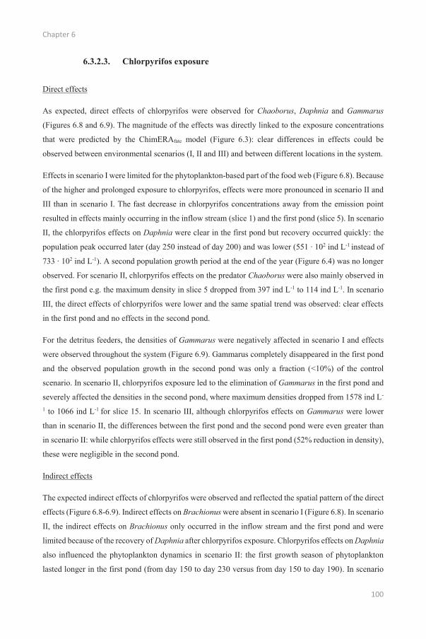
Chapter 6
100
6.3.2.3. Chlorpyrifos exposure
Direct effects
As expected, direct effects of chlorpyrifos were observed for Chaoborus, Daphnia and Gammarus
(Figures 6.8 and 6.9). The magnitude of the effects was directly linked to the exposure concentrations
that were predicted by the ChimERAfate model (Figure 6.3): clear differences in effects could be
observed between environmental scenarios (I, II and III) and between different locations in the system.
Effects in scenario I were limited for the phytoplankton-based part of the food web (Figure 6.8). Because
of the higher and prolonged exposure to chlorpyrifos, effects were more pronounced in scenario II and
III than in scenario I. The fast decrease in chlorpyrifos concentrations away from the emission point
resulted in effects mainly occurring in the inflow stream (slice 1) and the first pond (slice 5). In scenario
II, the chlorpyrifos effects on Daphnia were clear in the first pond but recovery occurred quickly: the
population peak occurred later (day 250 instead of day 200) and was lower (551 ∙ 102 ind L-1 instead of
733 ∙ 102 ind L-1). A second population growth period at the end of the year (Figure 6.4) was no longer
observed. For scenario II, chlorpyrifos effects on the predator Chaoborus were also mainly observed in
the first pond e.g. the maximum density in slice 5 dropped from 397 ind L-1 to 114 ind L-1. In scenario
III, the direct effects of chlorpyrifos were lower and the same spatial trend was observed: clear effects
in the first pond and no effects in the second pond.
For the detritus feeders, the densities of Gammarus were negatively affected in scenario I and effects
were observed throughout the system (Figure 6.9). Gammarus completely disappeared in the first pond
and the observed population growth in the second pond was only a fraction (<10%) of the control
scenario. In scenario II, chlorpyrifos exposure led to the elimination of Gammarus in the first pond and
severely affected the densities in the second pond, where maximum densities dropped from 1578 ind L-
1 to 1066 ind L-1 for slice 15. In scenario III, although chlorpyrifos effects on Gammarus were lower
than in scenario II, the differences between the first pond and the second pond were even greater than
in scenario II: while chlorpyrifos effects were still observed in the first pond (52% reduction in density),
these were negligible in the second pond.
Indirect effects
The expected indirect effects of chlorpyrifos were observed and reflected the spatial pattern of the direct
effects (Figure 6.8-6.9). Indirect effects on Brachionus were absent in scenario I (Figure 6.8). In scenario
II, the indirect effects on Brachionus only occurred in the inflow stream and the first pond and were
limited because of the recovery of Daphnia after chlorpyrifos exposure. Chlorpyrifos effects on Daphnia
also influenced the phytoplankton dynamics in scenario II: the first growth season of phytoplankton
lasted longer in the first pond (from day 150 to day 230 versus from day 150 to day 190). In scenario

The ChimERA model as a model analysis tool
101
III, indirect effects on Brachionus were again limited to the inflow stream and the first pond and only
resulted in a small increase in Brachionus density (<10%).
In scenario I, the densities of Gammarus were negatively affected but indirect effects on its competitor
Asellus were not observed (Figure 6.9). In scenario II, however, Asellus densities increased strongly
after chlorpyrifos emission in the inflow stream, first pond and connecting stream, leading to maximum
densities of 5708 ind L-1 in slice 5 versus 116 ind L-1 in the control scenario. The sharp population
decline in Asellus observed in the first pond around day 250 was a result of starvation. In scenario III,
the spatial pattern of the direct effects on Gammarus was confirmed and (low) indirect effects of
chlorpyrifos on Asellus were observed in slices 1 and 5 only.

Chapter 6
102
Fig
ure
6.8:
Foo
d w
eb d
ynam
ics w
ith c
hlor
pyri
fos e
xpos
ure
as p
redi
cted
by
the
Chi
mER
A m
odel
for t
hree
env
iron
men
tal s
cena
rios
(sce
nari
os
I, II
and
III)
and
four
sele
cted
loca
tions
in th
e tw
o-po
nd s
yste
m: a
t the
inflo
w o
f the
firs
t pon
d (S
lice
1), i
n th
e m
iddl
e of
the
first
pon
d (S
lice
5), b
etwe
en th
e tw
o po
nds
(Slic
e 10
) and
in th
e m
iddl
e of
the
seco
nd p
ond
(Slic
e 15
). O
nly
the
phyt
opla
nkto
n-ba
sed
part
of th
e fo
od w
eb is
sh
own.
Lin
es a
nd sh
aded
are
as in
dica
te th
e av
erag
e an
d m
inim
um a
nd m
axim
um d
ensi
ties,
resp
ectiv
ely,
of f
ive
itera
tions
per
scen
ario
.
( ~-1 MM 6W) UOptUeidOlÁ4d SL'O S'O SZ'O 0 I SL'O S'O SZ'O 0 I SL'O S'O SZ'O
~ I{) ~ ..-- ~
~
~
w ~ ü ::i ~ (/)
~
~
c J
~
~
~
§ ~ ê c: ost osz OSI os 0 009 009 00> ooz OOSI 0001 oos .9
"' c: SL'O s·o sz·o SL'O s·o sz·o SL'O s·o sz·o "' ä.
~ ~ 0
~ >. .t::. a.
0 ~ ..--w ~ ü __J ~
~ ~
~
~
~
~
~ (/)
~
§
~
ê
.!,!!
~ c: .c: - g. § ~ 0
ost osz OSI os 0 009 009 00> ooz OOSI 0001 oos Q)
SL'O s·o sz·o SL'O s·o sz·o SL'O s·o sz·o E F
~
I{) ~ w ~ ü
~
~ 2: ~
~ ., ;::
~ 2 0
"' ~ .c: ü
::i ~ (/)
~
~ .:- .f..
~
~
~
§ ost osz OSI os 0 009 009 001> ooz
ê l OOSI 0001 oos
ê ~ c: .Q '5
SL'O s·o sz·o SL'O s·o sz·o SL'O s·o sz·o ~ IXl
~ ~ ~
..-- ~ ~ ~ w ~ ü ~ ~
::i ~ (/) ~ ~
~ ~ ~
§ ê § ost osz OSI os 0 009 009 001> ooz OOSI 0001 oos
a~uepunqv
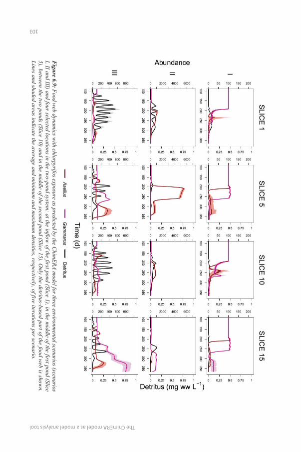
The ChimERA model as a model analysis tool
103
Figure 6.9: Food w
eb dynamics w
ith chlorpyrifos exposure as predicted by the Chim
ERA model for three environm
ental scenarios (scenarios I, II and III) and four selected locations in the tw
o -pond system: at the inflow
of the first pond (Slice 1), in the middle of the first pond (Slice
5), between the tw
o ponds (Slice 10) and in the middle of t he second pond (Slice 15). O
nly the detritus-based part of the food web is shown.
Lines and shaded areas indicate the average and minim
um and m
aximum
densities, respectively, o f five iterations per scenario.
Abundance
- - -0 200 400 600 800 0 2000 4000 6000 0 50 100 150 200
8 8 8
~ ~ ~
;jF (/) 8 8 r
~ ~ 0 m
8 8 ...... 8
~ ~ ~
0.25 0.5 0.75 1 0 0.25 0.5 0.75 1 0 0.25 0.5 0.75
0 200 400 600 800 0 2000 4000 6000 0 50 100 150 200
8 8 8
~ ~ ~ ):.
8 8 :jp (/)
"' r tb
d ê' ~ ~
0 "' m
8 8 1 CJ1
~ ~ ~ G) -i Q)
~ï 0 0.25 0.5 0.75 1 0 0.25 0.5 0.75 1 0 0.25 0.5 0.75 3
3 ct> 0 200 400 600 800 0 2000 4000 6000 0 50 100 150 200 Q)
2 "' 0: 8 8 8 ._..
~ ~
~ j~ (/)
0 8 8
~ r
~ "' ()
Ë ~ ~ m (/1 ......
8 8 0
~ ~ ~
0.25 0.5 0.75 1 0 0.25 0.5 0.75 1 0 0.25 0.5 0.75
0 200 400 600 800 0 2000 4000 6000 0 50 100 150 200
8 8 8
~ ~ ~ (/)
8 8 8 r 0
~ ~ ~ m ......
8 8 8 CJ1
~ ~ ~
0.25 0.5 0.75 1 0 0.25 0.5 0.75 1 0 0.25 0.5 0.75
Detritus (mg ww L-1)

Chapter 6
104
6.3.2.4. Pyrene exposure
Direct effects
In scenario I, Daphnia population dynamics exposed to pyrene (Figure 6.10) followed the same pattern
as in the control scenario (Figure 6.4). However, the maximum observed densities of Daphnia were
lower than those in the control scenario (131 ∙ 102 ind L-1 versus 205 ∙ 102 ind L-1). In scenario II and
especially scenario III, effects on Daphnia were higher than in scenario I and eventually daphnids were
eliminated from the food web. Following the exposure pattern, effects occurred first close to the
emission point (slice 1). Direct effects on Gammarus were absent (Figure 6.11): in none of the scenarios
was there a decrease in Gammarus densities that could be directly related to the pyrene concentration
and Gammarus concentrations were even higher in scenario III. The observed effects on Gammarus
were mainly indirect effects (see below).
Indirect effects
In scenario I, although expected, the decreased Daphnia densities did not lead to higher Brachionus
densities (Figure 6.10). In scenario II, the expected indirect effects of pyrene were observed: Brachionus
was clearly more abundant than in the control scenario and three peaks in density were observed
throughout the year. In scenario III, after the early disappearance of Daphnia, Brachionus was even
more dominant than in the control scenario: peaks in population density were even higher and the
number of peaks in density increased from 5 to 8. The predator Chaoborus was affected indirectly by
pyrene in all three scenarios through the lower prey density. In scenario I, Chaoborus densities decreased
from 314 ind L-1 in the control scenario to 158 ind L-1. Both in scenario II and III, despite the increase
in the other prey species Brachionus, Chaoborus disappeared once Daphnia was eliminated from the
food web by pyrene.
The combination of direct effects on Daphnia and indirect effects on Brachionus altered the
phytoplankton dynamics (Figure 6.10). This, in turn, affected the detritus dynamics, resulting in
unexpected indirect effects on the detritus feeders (Figure 6.11). In scenario I, the altered detritus
dynamics resulted in the absence of Gammarus population growth at the end of the year. In scenario II,
the phytoplankton concentration was more constant in the ponds between day 175 and 275, resulting in
more constant detritus concentrations and the absence of a peak in detritus concentrations compared to
the control scenario (Figure 6.5). This resulted in lower Gammarus densities (only 464 ind L-1 compared
to 1579 ind L-1 in the control scenario) but did not affect Asellus densities. In scenario III, the number
of phytoplankton growth periods increased from 6 to 9, which was reflected in the detritus dynamics.
As a result, both Gammarus and Asellus densities increased in comparison to the control scenario, from
1034 ind L-1 and 405 ind L-1 to 1401 ind L-1 and 545 ind L-1, respectively.
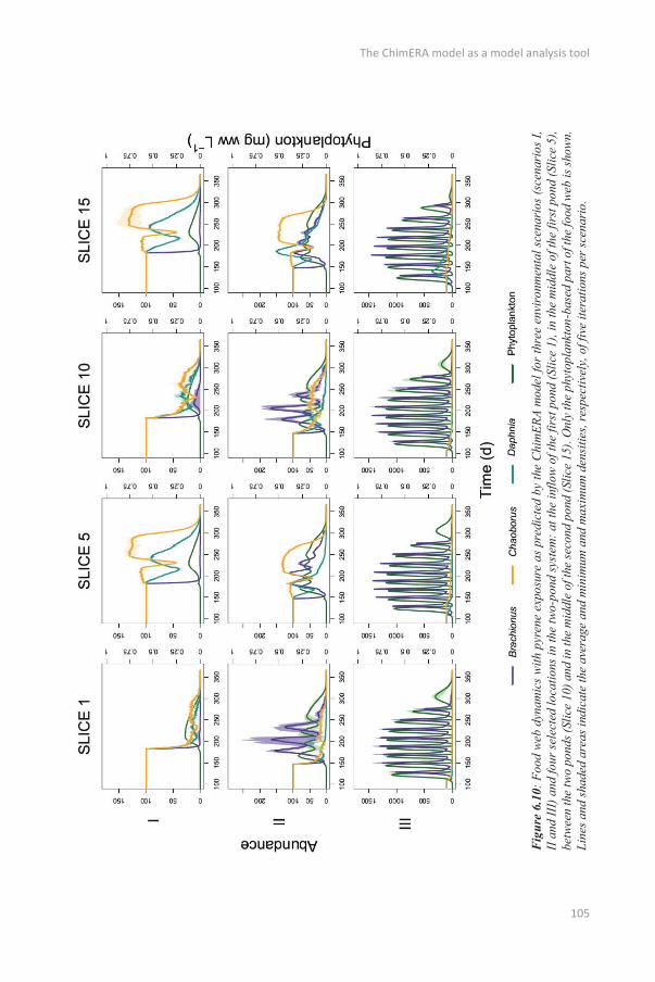
The ChimERA model as a model analysis tool
105
Fig
ure
6.10
: Foo
d w
eb d
ynam
ics
with
pyr
ene
expo
sure
as
pred
icte
d by
the
Chi
mER
A m
odel
for
thre
e en
viro
nmen
tal s
cena
rios
(sce
nari
os I,
II
and
III)
and
four
sele
cted
loca
tions
in th
e tw
o-po
nd sy
stem
: at t
he in
flow
of t
he fi
rst p
ond
(Slic
e 1)
, in
the
mid
dle
of th
e fir
st p
ond
(Slic
e 5)
, be
twee
n th
e tw
o po
nds (
Slic
e 10
) and
in th
e m
iddl
e of
the
seco
nd p
ond
(Slic
e 15
). O
nly
the
phyt
opla
nkto
n-ba
sed
part
of t
he fo
od w
eb is
show
n.
Line
s and
shad
ed a
reas
indi
cate
the
aver
age
and
min
imum
and
max
imum
den
sitie
s, re
spec
tivel
y, o
f fiv
e ite
ratio
ns p
er sc
enar
io.
( ~-1 MM 6W) UOptUeidOlÁ4d Sl'O s·o SZ'O 0 I Sl'O S'O sz·o 0 I Sl'O S'O SZ'O
~ ~ ~ I{) ~ ~ ~ ..--w ~ ~ ~ ü ::i ~ ~ ~ (/)
~ ~ ~
§ § § c:
OSI OOI os ooz OOI OS 0 OOSI 0001 oos .9 "' c:
Sl'O s·o SZ'O Sl'O s·o sz·o Sl'O s·o sz·o "' ä. 0
~ ~ ~ >. .t::. a.
0 ~ ~ ~ ..--w ~ ~ ~ ü __J ~ ~ ~ (/) .!,!!
~ ~ ~ c: .c: - g. § ê § ~ 0
OSI OOI os ooz OOI OS 0 OOSI 0001 oos Q)
Sl'O s·o SZ'O Sl 'O s·o sz·o Sl'O s·o sz·o E F
~ ~ ~ ., ;::
~ ~ ~ 2 I{) 0
"' w ~ ~ ~ .c: ü
ü ::i ~ ~ ~ (/)
~ ~ ~
§ ê ê ~ c: .Q
OSI OOI os ooz 00~ os 0 OOSI 0001 oos '5 Sl'O s·o SZ'O Sl'O s·o sz·o Sl'O s·o sz·o ~
IXl
~ ~ ~
..-- ~ ~ ~ w
~ ~ ~ ~ ü
::i ~ ~ ~ (/)
~ ~ ~
§ ê § OSI OOI os ooz OOI os 0 OOSI 0001 oos
a~uepunqv
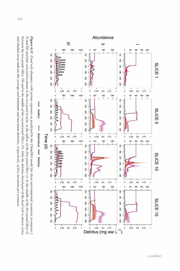
Chapter 6
106
Figure 6.11: Food w
eb dynamics w
ith pyrene exposure as predicted by the Chim
ERA model for three environm
ental scenarios (scenarios I, II and III) and four selected locations in the tw
o -pond system: at the inflow
of the first pond (Slice 1), in the middle of the first pond (Slice 5),
between the tw
o ponds (Slice 10) and in the middle of the second pond (Slice 15). O
nly the detritus -based part of the food web is show
n. Lines and shaded areas indicate the average and m
inimum
and maxim
um densities, respectively, of five iterations per scenario.
Abundance
- - -500 1000 1500 0 100 300 500 0 50 100 150 200
8 8 8
~ ~ ~
8 8 ; j~ (/) r
~ ~ 0 m
8 8 ...... 8
~ ~ ~
0.25 0.5 0.75 1 0 0.25 0.5 0.75 1 0 0.25 0.5 0.75
500 1000 1500 0 100 300 500 0 50 100 150 200
8 8 8
~ ~ ~ ):.
8 8 :JP (/)
"' r tb ê'
~ ~ 0
"' m 8 8 CJ1
~ ~ ~ G) -i Q)
~ï 0 0.25 0.5 0.75 1 0 0.25 0.5 0.75 1 0 0.25 0.5 0.75 3
3 ct> 0 500 1000 1500 0 100 300 500 0 50 100 150 200 Q)
2 "' 0: 8 8 8 ._..
~ ~
~ j~ . (/)
0 8 8 r ~ "'
() Ë ~ ~ m (/1 ......
8 8 0
~ ~ ~
0.25 0.5 0.75 1 0 0.25 0.5 0.75 1 0 0.25 0.5 0.75
500 1000 1500 0 100 300 500 0 50 100 150 200
8 8 8
~ ~
~ jp (/)
8 8 r 0
~ ~ m ......
8 8 CJ1
~ ~ ~
0.25 0.5 0.75 1 0 0.25 0.5 0.75 1 0 0.25 0.5 0.75
Detritus (mg ww L-1)

The ChimERA model as a model analysis tool
107
6.3.2.5. Exposure to the mixture of all three chemicals
Direct effects
In scenario I, the pattern in Daphnia densities was similar to the control scenario (Figure 6.4) but the
maximum densities were lower (Figure 6.12). In scenario II, Daphnia was eliminated quickly in the
whole system with effects appearing earlier close to the emission source (slice 1). Daphnia disappeared
from the first pond by day 200 and from the second pond by day 250. In scenario III, the effects of the
mixture occurred even faster, with Daphnia disappearing from the first pond by day 150.
For Gammarus in scenario I, direct effects of the mixture on the densities were limited and only occurred
after day 250 (Figure 6.13). In scenario II, the effects were more clear, although they only started
occurring after carbendazim and chlorpyrifos were first applied (day 180): Gammarus disappeared from
the system and this occurred first close to the emission point. Effects of the mixture on Gammarus were
also clear in scenario III but Gammarus was able to persist longer in the second pond compared to
scenario II.
Direct effects of the mixture for Chaoborus are expected to be similar to the direct effects of chlorpyrifos
as this species is tolerant for the other two chemicals. Direct effects of the mixture on Chaoborus
densities were not observed in scenario I (Figure 6.12). In scenario II, a sharp decrease in Chaoborus
density is observed in the first pond (slice 5) after the application of chlorpyrifos and carbendazim (day
180). Direct effects in the second pond were limited. In scenario III, direct effects of the mixture were
no longer observed and the population dynamics of Chaoborus were determined by the indirect effects
of the mixture (see below).
Indirect effects
For Brachionus in scenario I, the indirect effects were negligible (Figure 6.12) because the densities
were very similar to the control scenario (Figure 6.4). In scenario II, following the disappearance of
Daphnia after chemical exposure, densities of the tolerant Brachionus increased in all slices and showed
three distinct population peaks. In scenario III, indirect effects of exposure to the mixture of three
chemicals resulted in an increase in Brachionus densities. Also, the frequency of the peaks in Brachionus
density increased from 5 to 8 compared to the control scenario.
Through the strong direct and indirect effects of the mixture on the grazers, phytoplankton dynamics
were altered. Because of the close link between phytoplankton and detritus, this resulted in indirect
effects of the mixture on the detritus feeders. In scenario I, the altered detritus concentrations resulted
in the absence of Gammarus growth at the end of the year (Figures 6.5 and 6.13). This did, however,
not result in an increase in Asellus densities. In scenario II, the exposure to the mixture resulted indirectly
in increased Asellus densities in the whole system and this increase was highest in the first pond (slice

Chapter 6
108
5). In the case of scenario III, the increase of Asellus was only observed for the first pond. Also in
scenario III, because of the altered detritus dynamics, Gammarus was able to reach higher densities in
the second pond (1314 ind L-1) compared to the control scenario (1034 ind L-1).
In scenario I, Chaoborus densities were lower (Figure 6.12) than the control scenario (Figure 6.5)
because of the decreased densities of Daphnia. In scenario II, in addition to the direct effects of the
mixture, Chaoborus was indirectly affected through the effects on Daphnia and population densities
were never higher than 100 ind L-1. In scenario III, the effects of the mixture on Daphnia resulted in the
elimination of Chaoborus even before carbendazim and chlorpyrifos were applied (day 180).

The ChimERA model as a model analysis tool
109
Figure 6.12: Food w
eb dynamics exposed to three chem
icals as predicted by the ChimERA m
odel for three environmental scenarios (scenarios
I, II and III) and four selected locations in the two -pond system
: at the inflow of the first pond (Slice 1), in the m
iddle of the first pond (Slice 5), between the tw
o ponds (Slice 10) and in the middle of the second pond (Slice 15). O
nly the phytoplankton -based part of the food web is
shown. Lines and shaded areas indicate the average and m
inimum
and maxim
um densities, respectively, of five iterations per scenario.
Abundance
- - -500 1000 1500 0 50 150 250 350 0 50 100 150
8 8 8
~ ~ ~
8 8 ;jW (/) r 0
~ ~ m 8 8 ......
8
~ ~ ~ I
tiJ iiJ
0 0.25 0.5 0.75 1 0 025 0.5 0.75 1 0 0.25 0.5 0.75
g. 0 500 1000 1500 0 50 150 250 350 0 50 100 150 o· => 8 8 8 ~
~ ~ ~
8 8
: J~ (/) r
~ ~ 0
() m ::r Q)
CJ1 0 8 8 c::r 0 2 ~ ~ ~ "'
-i ~ï
0 0.25 0.5 0.75 1 0 025 0.5 0.75 1 0 0.25 0.5 0.75
ct> 0 500 1000 1500 0 50 150 250 350 0 50 100 150
I:J 0: 8 8 8 ~ -::r ~ ~
~ j~ =>
(/) iiï
8 8 r ()
"' ~ ~ m ......
8 8 0 -o
~ ~ ~ :::r 'S. 0 "0 iiï 0 0.25 0.5 0.75 1 0 0.25 0.5 0.75 1 0 0.25 0.5 0.75 ::>
" ö 0 500 1000 1500 0 50 150 250 350 0 50 100 150
::> 8 8 8
~ ~
~ j~ (/)
8 8 r 0
~ ~ m ......
8 8 CJ1
~ ~ ~
0.25 0.5 0.75 1 0 025 0.5 0.75 1 0 0.25 0.5 0.75
Phytoplankton (mg ww L -1)

Chapter 6
110
Figure 6.13: Food web dynamics exposed to three chemicals as predicted by the ChimERA model for three environmental scenarios (scenarios I, II and III) and four selected locations in the two-pond system: at the inflow of the first pond (Slice 1), in the middle of the first pond (Slice 5), between the two ponds (Slice 10) and in the middle of the second pond (Slice 15). Only the detritus-based part of the food web is shown. Lines and shaded areas indicate the average and minimum and maximum densities, respectively, of five iterations per scenario.
SLICE 1 SLICE 5 SLICE10 SLICE15 ~ ~ ~ ~
~ ~ ~ ~
~ !; ~ !; ~ !; ~ ..., 0
~ ~ ~ ~
ó ó ó ó
ê 8 8 8 ~ ~
\ 1~ ~ ~ ~ ~ ~
"' "' "' :;l ~ 0 ~ 0 ~ 0 ~
0 0 0 0 0 0 i I I I I
100 150 200 250 300 350 100 150 200 250 :300 350 100 150 200 250 300 350 100 150 200 250 300 350 .-I
~ ...J
Q)
:1 K! ~
F1 f 2 I
fH1 f;! (.)
c ó
ro ~ 8 ~ 8 "0 11 ei "' ei "'
_{1 :;J E c -:::J liJ 8 liJ 8 liJ C/) .0 b. <( ,.1\ 1'.~
ei ~ ei ~
~ ei :::J -' ï ::::: 0 -
Q) 100 150 200 250 300 350 100 150 200 250 300 350 100 150 200 250 300 350 100 150 200 250 300 350 0
0
~ - ~ ~ ~ - ~ i!? i!? i!?
r , ó ó ó ó
:t~ 8 8 8
111 \t) ~ ~ :!! ~ :!! ~
ei ei ei ei
~ § ~ ~ ~ ~ liJ ei
0 0 0 0 0 0
100 150 200 250 300 350 100 150 200 250 300 350 100 150 200 250 300 350 100 150 200 250 300 350
Time (d)
- Aseflus - Gammarus - Delritus
The ChimERA model as a model analysis tool
111
6.4. Discussion
6.4.1. ChimERAfate simulations
When comparing the fate model predictions among the different scenarios, the residence time –reflecting
the removal of the chemical from the ponds via with the water (out)flow – was the most important factor.
Higher residence times resulted in less dilution of the chemical i.e. more chemical was emitted in the
same volume of water. This explains why higher water concentrations were observed (for all chemicals)
in scenario III (residence time of 100 days) compared to the concentrations in scenario II and I (residence
time of 25 and 5 days, respectively). As discussed in the expectations section (6.2.2.1), sediment
accumulation of the chemical also increased with water residence time, decreasing the concentration in
the water. Apparently, sediment accumulation was not strong enough to compensate for the positive
effect of retention time on the water concentration. However, the effects of sediment accumulation were
visible in the spatial patterns within the system: because most of the chemical accumulated in the
sediment, the water concentrations of the hydrophobic chemical chlorpyrifos were much lower in the
second pond than in the first pond and this was more expressed in scenarios with long residence times.
The expected negative effect of a higher temperature – and the resulting increased phytoplankton and
detritus biomass – and a higher organic matter concentration on the water concentration were not
observed. These two processes were apparently not strong enough to compensate for the positive effect
of a higher residence time.
The fate simulations for carbendazim differed substantially from the expectations (6.2.2.1). Despite the
short peaks in emission, concentrations remained high for much longer than expected further away from
the emission point in scenarios with higher residence times. Although no accumulation in sediment
occurred for this hydrophilic chemical, diffusion into the sediment pore water and later again into the
water column was an important fate process for carbendazim. This allowed for more constant dissolved
water concentrations. More time for equilibrium between the sediment pore water and the water column
was available in systems with high water residence times. This resulted in more diffusion into the
sediment, explaining the stronger decrease in carbendazim water concentration further downstream in
scenarios III than in scenario II and I.
As expected, because of the hydrophobic nature of chlorpyrifos, accumulation in the sediment occurred
and this led to constant water concentrations even when emission had stopped. This was best visible in
slice 1, where the emission occurred: once emission stopped, the water concentration quickly decreased
to a low but relatively constant ambient concentration. Because most of the chlorpyrifos accumulated in
the sediment, maximum chlorpyrifos concentrations were lower and reached later further downstream
in the system, especially in scenarios with high water residence time. Simulated pyrene concentrations
Chapter 6
112
became stable over time, as expected, because of the constant emission strength. Water residence time
and sediment accumulation determined how fast water concentrations stabilized: the emitted pyrene
flowed downstream slower with increased water residence time and accumulation in the sediment
further prolonged the stabilization of the water concentrations.
With the ChimERAfate model, we clearly showed that spatiotemporal differences in exposure were
determined by the physico-chemical properties of the chemical and the environmental variables
considered here (hydrodynamics, trophic state and temperature). Although environmental fate processes
are well studied and can be described accurately with equations, the predicted patterns in exposure
sometimes differed from our expectations e.g. for carbendazim. The relative importance of each
environmental process is not always clear a priori and can change with the environmental conditions.
Fate models are thus ideal tools to identify which chemicals will show a strong spatial pattern and in
which environmental conditions spatial patterns will be most prominent. Identifying whether chemicals
will only be present in high concentrations close to the emission source or also further downstream is
an invaluable tool to predict the risk of the chemical.
6.4.2. ChimERAfoodweb without chemical exposure
Both phytoplankton growth and maximum phytoplankton concentration increased with the increase in
trophic state and temperature. As a result, grazer densities increased rapidly in eutrophic, high
temperature environments such as scenario III. The higher trophic state and temperature in scenario III
compared to the other two scenarios also led to a more dynamic system, with a typical cyclic pattern of
phytoplankton growth, increase in grazer densities, phytoplankton decline and decrease in grazer
densities. These faster food web dynamics in mesotrophic systems compared to those in oligotrophic
systems were predicted before for a similar food web using ordinary differential equations to describe
the biomass of the species in the food web (De Laender et al. 2015). Because Brachionus has a much
shorter life cycle than Daphnia, the rotifers were able to increase in density more rapidly during
phytoplankton growth periods, leading to the observed shift in dominance in scenario III compared to
scenario I and II. However, this does not seem to reflect observations in real ecosystems, where daphnids
are known to outcompete rotifers (Gilbert 1985; MacIsaac and Gilbert 1989). Other competitive
mechanisms between large daphnids and rotifers have been suggested in literature e.g. through
mechanical interference (MacIsaac and Gilbert 1989). As shown in Chapter 4, accounting for
competitive exclusion was sufficient to simulate the outcome of competition between Daphnia magna
and Brachionus calyciflorus for the experimental conditions used in Chapter 2. However, alternative
mechanisms of competition could be more important when environmental conditions are more realistic
than the controlled conditions used in Chapter 2. Because the relative importance of such alternative
modes of competition was not known, they were therefore not implemented in the DEBkiss IBMs.

113
The current food web dynamics are clearly bottom-up regulated: grazer dynamics were limited by the
phytoplankton, detritus feeders followed the detritus pattern and prey dynamics. Although they are able
to prey on both Brachionus and Daphnia, Chaoborus was most abundant when Daphnia was dominant
i.e. in scenario II. Seemingly, Chaoborus was thus not able to sustain high population densities in
scenario III when maximum Brachionus densities were high. However, Brachionus densities also
fluctuated strongly in scenario III. The lower Chaoborus densities in scenario III were probably related
to the absence of a reserve compartment in the DEBkiss theory. When prey populations were high,
energy uptake by Chaoborus was also high and this energy was immediately spent. When prey densities
were low, the energy uptake by Chaoborus was insufficient. In reality, Chaoborus would first utilize
energy from the reserve buffer in that situation (Kooijman 2010). However, since a reserve compartment
is lacking in DEBkiss, energy is instead taken from the reproduction buffer or, when all energy in the
reproduction buffer is spent, from structural biomass. This led to a much faster response to food shortage
compared to reality, as discussed in Chapter 4. Daphnids show much less extreme population dynamics,
serving as better prey species for the Chaoborus DEBkiss IBM.
Even without chemical exposure, there were notable spatial differences in food web dynamics: except
for Brachionus, population densities were lower in the streams than in the ponds. This is a direct result
of the way movement was implemented. Movement was implemented as a species-specific chance to
move to a neighbouring water patch. Patches located in a pond were surrounded by more water patches
than patches in a stream. Patches in a pond thus had a higher chance of receiving new individuals than
patches in a stream. This results in highly different population dynamics between ponds and streams for
mobile species. For example, the probability for Daphnia 1 to move to a neighbour water patch was 1 d-
1. As a result, daphnid density was much higher (e.g. up to five times for scenario II) in ponds than in
streams. The lower Daphnia and Chaoborus densities in the streams meant less competition and
predation pressure, allowing Brachionus, which had a lower movement chance (0.1 d-1), to reach higher
densities in the streams than in the ponds e.g. up to two times higher for scenario II.
6.4.3. ChimERAfoodweb with chemical exposure
The magnitude of effects was directly linked to the concentrations that were predicted by the
ChimERAfate model: clear differences in effects could be observed between the different environmental
scenarios (I, II and III) and between the different locations in the system. Recovery of the phytoplankton-
based part of the food web was observed for chlorpyrifos and carbendazim after the first emission peak
(around day 200). The second emission peak, combined with the decreased food availability and the
increased competition with the tolerant species (Brachionus), prevented recovery during the simulated
period. Unsurprisingly, recovery was not observed for pyrene exposure because the concentration was
relatively constant throughout the year. Recovery of the detritus-based part of the food web was
observed to be much more difficult. This was mainly due to the longer reproduction times of the detritus

Chapter 6
114
feeders: i.e. these were at least 40 and 80 days between reproduction events for Gammarus and Asellus,
respectively. Slower recovery of species with long life cycles or generation times has been raised as a
concern for ERA before (De Lange et al. 2010; Rubach et al. 2010). By including species with different
life cycle times or by adjusting the currently implemented generation times, the ChimERA model can
be a tool to assess how life cycle duration affects food web recovery.
Simulations performed using the ChimERA model showed a strong spatial pattern, with effects of
chemicals being absent, smaller or delayed in the second pond compared to those observed in the first
pond. A good example of the absence of effects in the second pond is the exposure to chlorpyrifos in
scenario II: the water concentrations in the first pond clearly caused a delay in daphnid population
growth while the food web dynamics in the second pond were completely unaffected. Smaller effects in
the second pond than in the first pond were, for example, observed for carbendazim in scenario III:
Gammarus densities were less affected in the second pond compared to the first pond. Delayed effects
were clearly visible for pyrene in scenario III: Daphnia populations in the second pond also became
extinct but this occurred much later than in the first pond. Also, because Daphnia and Chaoborus tended
to remain in the ponds and were much less abundant in the streams, the food web dynamics in the streams
were already more determined by the tolerant Brachionus and effects of the chemical were generally
less severe there. This highlights the need in a spatial landscape to account for the local conditions.
Environmental variables such as temperature, light conditions and water flow strength are distributed
heterogeneously in a landscape. Environmental conditions determine which species are successful and
local food webs can thus differ greatly in their structure and composition. Chemical risk for a landscape
is not homogeneously distributed but local differences will exist because exposure and food web
vulnerability differ locally. The ChimERA model, although only applied here for a two-pond system, is
a good example of how an integrated fate and effect model can be used to differentiate the local risks
within a spatial system.
Indirect effects were prevalent in the ChimERA simulations and included indirect effects on
competitors, on predators and on a food source (i.e. phytoplankton and detritus). Chemical effects on
the sensitive species often led to increased densities of the tolerant species which became dominant in
some cases. Especially the indirect effect of chlorpyrifos on Asellus densities in scenario II was striking.
Brachionus typically also increased in density after chemical effects on Daphnia had occurred. This
effect was, however, less drastic than those observed on Asellus and mainly occurred in scenario II. In
scenario I, rotifers were quickly outcompeted by the daphnids, even before chemical effects became
apparent, preventing possible indirect effects on Brachionus. In scenario III, rotifers were already quite
high in density and indirect effects only resulted in small increases in density. A shift in dominance
between competitors is often observed after chemical exposure. For example, increases in rotifer
abundance after chemical effects on cladocerans were observed after the application of fenvalerate in
lake enclosures (Day et al. 1987). However, rotifers can also be outcompeted by cladocerans after

115
chemical exposure e.g. the cladoceran Moina macrocopa outcompeted the sensitive rotifer Brachionus
calyciflorus after exposure to cadmium (Gama-Flores et al. 2006). Other examples of shifts in
dominance after chemical exposure include the replacement of green algae by cyanobacteria and
diatoms after fomesafen application (Caquet et al. 2005) or the increase in tolerant rotifers species after
carbendazim effects on cladocerans and copepods (Van den Brink et al. 2000). Theoretically, it makes
sense that an inferior competitor can be successful when the superior competitor is affected by chemical
stress because less resources are consumed by the superior competitor. However, this is not always
observed in experiments (Chapter 2). In the ChimERA simulations, even when the superior competitor
was affected, other conditions were also important. For example, in the simulations performed for
pyrene exposure in scenario I, effects of pyrene on Daphnia densities were not sufficiently high to
prevent the elimination of Brachionus. Also, the food concentrations in scenario I were too low to sustain
high densities of Brachionus, which was demonstrated in the streams where competition with Daphnia
was almost absent but where Brachionus densities were still close to zero. Models like the ChimERA
model can help to understand and predict when and why indirect effects occur.
Indirect effects of carbendazim and pyrene were observed on the predator Chaoborus. Although the
maximum densities of Brachionus increased after chemical exposure, these rotifer densities fluctuated
much more than Daphnia densities. With the current Chaoborus DEBkiss IBM implementation, it was
difficult to simulate stable population densities when food availability is highly dynamic, as discussed
before (see 6.4.2). Because of the high fluctuations in Brachionus densities, Brachionus was thus a less
suitable prey for Chaoborus, leading to the observed indirect effect on Chaoborus densities: reduced
population densities when Daphnia density was negatively affected by chemical stress and even
extinction e.g in the case of pyrene exposure in scenario III. Altered Daphnia densities due to chemical
stress lowered the Chaoborus densities but could also lead to a longer period of stable predator densities
when daphnid densities recovered from chemical exposure e.g. after carbendazim exposure in scenario
II.
Phytoplankton is the only source of detritus in the fate model. Therefore, it is expected that a chemical
exposure affecting grazer dynamics will lead to changes in phytoplankton dynamics and as a result, in
different detritus dynamics. For example, due to the pyrene exposure in scenario II, the phytoplankton
dynamics shifted from two distinct peaks at day 175 and 250 in the ponds to a more constant
phytoplankton concentration with four smaller peaks between day 150 and 250. This resulted in different
detritus dynamics, ultimately also affecting the detritus feeders, in this case by preventing the strong
increase in Gammarus density at the end of the year. Interestingly, shifts in grazer densities did not
necessarily affect the detritus feeders negatively. For pyrene in scenario III for example, the dominance
shift to Brachionus increased the amount of detritus available, resulting in higher Asellus and Gammarus
densities. In reality, however, the main food sources of Asellus and Gammarus are not from
phytoplankton origin. The diet of Asellus and Gammarus is much more diverse with leaf litter from

Chapter 6
116
external sources (terrestrial plants) often cited as the most important food source (Moore 1975). This
was not considered in the ChimERA model and Asellus and Gammarus were thus much more dependent
on phytoplankton dynamics than in reality. However, this did allow us to study the interactions between
phytoplankton, detritus and associated consumers.
For the grazers and predator in the food web, the overall effect(s) of the mixture seemed to be dominated
by the effects of pyrene: effects of the mixture on the grazers corresponded mostly with the effects of
pyrene alone, with effects occurring almost immediately after the start of the simulated exposure. For
the detritus feeders, however, this was not the case: direct effects of pyrene on Gammarus were limited
in the pyrene only exposure, but effects of the mixture were clearly visible leading to a dominance of
Asellus. Identification of the dominant chemical in the mixture was done by comparing which effects of
the single exposure corresponded most to the effects of the mixture. For more complex food web models
or mixtures, where more effects can occur, this approach is insufficient and alternative approaches need
to be considered e.g. similarity indices such as the Bray-Curtis index (Bray and Curtis 1957). Similarity
indices describe the composition of the community/food web with a single number. For example, the
Bray-Curtis indices of the communities exposed to the mixture and of those exposed to the chemicals
in the mixture individually could be compared. The Bray-Curtis index of the individual chemical closest
to the index of the mixture then indicates in which community the effects of the individual chemical are
most similar to the effects of the mixture i.e. which effect dominates.
Mixture toxicity at the community level can be very different from mixture toxicity at the level of
individuals and populations. For example, the effects of a herbicide and an insecticide, affecting
phytoplankton and grazers, respectively, are not necessarily additive (i.e. the sum of the individual
effects) at the food web level. Synergistic effects at the food web level (i.e. higher effects than what is
expected from the individual effects) could occur when the grazers are affected both by direct effects of
the insecticide and by indirect effects due to herbicide effects on the phytoplankton. Antagonistic effects
(i.e. smaller effects than what is expected from the individual effects) could occur when the
phytoplankton is affected by the herbicide but is less grazed upon because of the adverse insecticide
effects on the grazers. Models like the ChimERA model offer a unique way to account for this.
6.4.4. The ChimERA model as a risk assessment tool
The ChimERA model demonstrates how integrating a fate and food web model offers insights that
cannot be obtained when running both models separately. Experimental/field data to compare our model
simulations with were not available. However, the underlying models – ChimERAfate and
ChimERAfoodweb – have been tested: the ChimERAfate model was successfully applied in three case
studies for a pond system (Morselli et al. 2015) and the application of the DEBkiss IBMs for competing
species – used in the ChimERAfoodweb model –was evaluated in Chapter 4. The simulations of the
117
ChimERA model were therefore considered realistic although it cannot be excluded that certain
processes or mechanisms important for the integrated model were not incorporated.
The ChimERA model can be seen as a proof of principle study of how a coupled fate and effect model
can be used as a realistic risk assessment tool incorporating more ecological and fate processes. The
uniqueness of the ChimERA model is that it used the input of various abiotic and biotic variables and
translated these into food web dynamics that varied greatly between the selected scenarios. This makes
models such as the ChimERA model ideally suited to address the question of multiple stressors (SCHER
et al. 2013; Gunderson et al. 2016): the ChimERA model provides an integrated prediction of all the
stressors present in the environment. Although the ChimERA model should be further improved with
e.g. additional environmental stressors (see 7.6), the integrated model (1) was able to provide realistic
effects of chemicals on food web dynamics based on the modelling of individual species, (2) included
spatiotemporal differences in exposure and effects on food web dynamics, (3) showed how the effects
of a chemical depend on the selected scenario, (4) included a feedback mechanisms between the abiotic
and biotic part of the system, (5) implemented an effect model capable of taking exposure history into
account and (6) considered the simultaneous effect of multiple chemicals.
(1) Realistic effects of chemicals on food web dynamics
Starting from the effects of a chemical assessed under laboratory conditions, the ChimERA model was
able to suggest how the chemical affects a hypothetical food web, taking into account both direct and
indirect effects. Indirect effects, occurring through competition and predation, need to be accounted for
in realistic ecological risk assessments (Fleeger et al. 2003). Indirect effects are very difficult to predict
based on single species toxicity tests alone and are difficult to account for in mesocosm studies (Van
den Brink and Ter Braak 1998). Ecological models have been suggested as good alternatives to account
for these indirect effects (Galic et al. 2010) and the ChimERA model demonstrated here how this can
be achieved: Asellus and Brachionus became dominant after chemical effects on Gammarus and
Daphnia, respectively, and the predator Chaoborus was negatively affected by chemical effects on its
prey Daphnia.
(2) Spatiotemporal differences in exposure and effects on food web dynamics
Although typically ignored in ecological risk assessments, the spatial structure of the system and the
location of emission can influence the effects of a chemical, e.g. as observed in mesocosms (Brock et
al. 2009) and predicted by models (Galic et al. 2012). Spatial structure will determine where and when
exposure is occurring (Wickwire et al. 2011), what fraction of the system is affected by the chemical
(Brock et al. 2009) and how fast the system can recover e.g. through immigration of biota from
unaffected locations (Dohmen et al. 2015). Because the spatial structure is explicitly taken into account
in the ChimERA model, the effects of the tested chemicals clearly differed between different locations
Chapter 6
118
in the system. The spatial dimension was not only important for differences in exposure. Differences in
food web structure in different parts of the system were also observed.. For example, as a result of
differences in movement potential of the different organisms, rotifers were more abundant and daphnids
less abundant in the streams than in the ponds.
(3) The outcome of chemical exposure depends on the selected scenario
Although the amount of chemical emitted to the system was identical in all scenarios, exposure
concentration and thus effects on the food web dynamics were highest in scenario III. The ChimERA
model was able to translate differences in environmental variables to differences in (1) food web
dynamics and (2) effects of chemical exposure. The three environmental scenarios studied here were
only a limited selection of the many possible combinations of temperature, trophic state and
hydrodynamics. Because of its flexibility, the ChimERA model structure can be tailored to specific real-
world situations by adjusting these environmental inputs. Similarly, the structure of the food web and
the species involved are exchangeable, thus allowing for adjustments to site-specific communities. The
scenarios studied here were limited to one spatial pattern i.e. two connected ponds. However, the
ChimERA model can be used to simulate scenarios for any kind of spatial structure and can thus be
applied to answer specific questions. For example, it could be used to assess how the presence of a non-
exposed part of the system affects the recovery of the food web.
The large number of possible scenarios can be confusing for risk assessors who need to decide e.g. if
the selected scenarios are applicable and/or if the food web and species are realistic. During the
development of Chimera, a similar problem was encountered for exposure assessment where there was
also a multitude of environmental fate models and scenarios available. To solve this, environmental
modelling was standardized and the FOCUS scenarios were developed (FOCUS 2001). A similar
standardization of ecological and effect models will help facilitate the acceptance of ecological models
as tools for effect assessment.
(4) Feedback mechanisms between the abiotic and biotic component of the system
The typical separate assessment of the fate and effects of chemicals ignores the fact that the
environmental fate is also influenced by the biological/ecological component of the system, and vice
versa. For example, the biomass of phytoplankton is an important factor for determining the bioavailable
concentration of a hydrophobic chemical (Morselli et al. 2015). However, phytoplankton is also a
component of the food web as it is consumed by grazers. Strong grazing pressure will limit the amount
of phytoplankton biomass in the system thus reducing the accumulation of the chemical in the
phytoplankton. The impact of this feedback mechanism was limited for the scenarios chosen here
because the effect of phytoplankton biomass on the chemical concentrations was limited. Other
biological compartments like macrophytes (Morselli et al. 2015) and zooplankton (Turner 2002) have

119
been shown to influence the environmental fate of a chemical significantly and can be included in future
scenarios.
(5) Effects of chemicals take earlier exposure into account
A TKTD model was used to predict the effects of chemicals on the survival of individuals. The nature
of this type of model allows effects to occur even when the environmental concentration of the chemical
have already decreased. This was visible e.g. for Daphnia exposed to chlorpyrifos in scenario II (Figure
6.8): at day 200, chlorpyrifos concentrations in the system had dropped to almost background
concentrations but adverse effects persisted and a population increase was only observed after day 210.
Although not tested here, TKTD models are especially useful when the emission is highly dynamic
(Jager et al. 2011). Even for chemicals that are emitted very irregularly, the TKTD approach is able to
predict the effects when only information of a typical toxicity test is available i.e. short term exposure
to a constant concentration.
(6) Simultaneous effects of multiple chemicals
The current implementation of the ChimERA model is able to predict the effects of a mixture of
chemicals, although the validity of the used mixture model is uncertain for the chemicals used in this
study. Mixture toxicity is complex and the selection of the appropriate mixture toxicity model depends
on the chemicals involved, although concentration addition was the preferred model in over 90% of
pesticide mixtures (Deneer 2000). The mechanisms of mixture toxicity between carbendazim,
chlorpyrifos and pyrene are unknown and an appropriate mixture toxicity model could therefore not be
chosen. The mixture toxicity model used here, although possibly invalid, did allow us to explore how
mixture toxicity effects may affect food web dynamics in comparison with single substance exposures.
Interestingly, different chemicals impacted different species: Daphnia was mainly affected by pyrene
while the effects of carbendazim and chlorpyrifos mainly affected Gammarus. Assessing the effects of
multiple chemicals on the food web is an important feature of the ChimERA model. Traditionally,
mixture toxicity studies focus on effects on the same organism. With the ChimERA model, mixture
toxicity effects can be evaluated for the whole food web. For example, how will the food web be affected
by the simultaneous exposure to a chemical affecting the grazers and one affecting the predators? The
ChimERA model can provide an answer to such a question by e.g. predicting that the negative effects
on the grazers are compensated by the reduced predation pressure, resulting in negligible effects of the
mixture on the grazer density.
Ecological risk assessment needs new methods to deal with the large amount of chemicals to which
ecosystems are possibly exposed and the increasing number of stressors that can interact with the effects
of a chemical (SCHER et al. 2013; Gunderson et al. 2016). Modelling has been named as one of the
most promising tools to face these challenges (SCHER et al. 2013). The simulations performed here
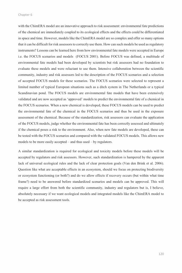
Chapter 6
120
with the ChimERA model are an innovative approach to risk assessment: environmental fate predictions
of the chemical are immediately coupled to its ecological effects and the effects could be differentiated
in space and time. However, models like the ChimERA model are so complex and offer so many options
that it can be difficult for risk assessors to correctly use them. How can such models be used as regulatory
instruments? Lessons can be learned here from how environmental fate models were accepted in Europe
i.e. the FOCUS scenarios and models (FOCUS 2001). Before FOCUS was defined, a multitude of
environmental fate models had been developed by scientists but risk assessors had no foundation to
evaluate these models and were reluctant to use them. Intensive collaboration between the scientific
community, industry and risk assessors led to the description of the FOCUS scenarios and a selection
of accepted FOCUS models for these scenarios. The FOCUS scenarios were selected to represent a
limited number of typical European situations such as a ditch system in The Netherlands or a typical
Scandinavian pond. The FOCUS models are environmental fate models that have been extensively
validated and are now accepted as ‘approved’ models to predict the environmental fate of a chemical in
the FOCUS scenarios. When a new chemical is developed, these FOCUS models can be used to predict
the environmental fate of the chemical in the FOCUS scenarios and thus be used in the exposure
assessment of the chemical. Because of the standardization, risk assessors can evaluate the application
of the FOCUS models, judge whether the environmental fate has been correctly assessed and ultimately
if the chemical poses a risk to the environment. Also, when new fate models are developed, these can
be tested with the FOCUS scenarios and compared with the validated FOCUS models. This allows new
models to be more easily accepted – and thus used – by regulators.
A similar standardization is required for ecological and toxicity models before these models will be
accepted by regulators and risk assessors. However, such standardization is hampered by the apparent
lack of universal ecological rules and the lack of clear protection goals (Van den Brink et al. 2006).
Question like what are acceptable effects in an ecosystem, should we focus on protecting biodiversity
or ecosystem functioning (or both?) and do we allow effects if recovery occurs (but within what time
frame?) need to be answered before standardized scenarios and models can be approved. This will
require a large effort from both the scientific community, industry and regulators but is, I believe,
absolutely necessary if we want ecological models and integrated models like the ChimERA model to
be accepted as risk assessment tools.

121
7 GENERAL CONCLUSIONS AND FUTURE
RESEARCH SUGGESTIONS

Chapter 7
122
7.1. Introduction
To perform adequate ecological risk assessment for the large amount of chemicals produced each year,
appropriate methods and procedures reflecting the environmental diversity and reality are needed.
Overall, current methods are, however, inadequate and lack ecological realism. New methods are
therefore needed and the use of ecological models has been suggested as a powerful tool to improve
ERA. In this PhD thesis the potential role of ecological interactions, one of the key characteristics
lacking from current ERA methods, was first studied experimentally. Individual based models (IBMs)
were then developed to simulate and evaluate the patterns observed in these experiments. Next, the
developed IBMs were integrated with an environmental fate model into the ChimERA model, capable
of simulating spatially-explicit effects of chemicals on a food web in realistic conditions. Finally, the
ChimERA model was tested as a scenario analysis tool.
The results of this PhD thesis are summarized in this chapter and suggestions for future research are
given. Each paragraph starts with the research question addressed in each chapter, then presents a
summary of the conclusions and finally suggests possible future research directions.
7.2. Species interactions and chemical stress: combined effects of intra- and
interspecific interactions and pyrene on Daphnia magna population
dynamics
The main research question addressed in Chapter 2 was how interactions within and between species –
intra- and interspecific competition with Brachionus calyciflorus and predation by Chaoborus sp. larvae
– influenced the effects of pyrene on populations of Daphnia magna.
Exposure to pyrene led to decreased D. magna densities and pyrene predominately affected smaller
individuals. Predation pressure by Chaoborus sp. larvae and intraspecific competition limited the D.
magna population densities but competition with B. calyciflorus had no significant effects on D. magna.
Predation pressure and intraspecific competition altered the size structure of the D. magna population,
reducing the fraction of small, more sensitive individuals in the population. As a result, predation and
intraspecific competition both interacted antagonistically with pyrene exposure i.e. reduced the effects
of pyrene. It can be concluded that, overall, interactions within and between species altered the effects
of pyrene, highlighting the need to account for such interactions in ecological risk assessments.
Future research suggestions: D. magna is a much stronger competitor and quickly outcompetes B.
calyciflorus in the used system. Probably, the influence of interspecific competition on the effects of a
chemical depends on the strength of the competition. How the strength of competition alters the effect

General conclusions and future research suggestions
123
of the chemical can be studied by e.g. using a smaller daphnid species. Similarly, the strength of the
predation pressure is expected to alter the effects of chemical exposure. This interaction can be studied
by using different predator species or densities. The effects of pyrene only became apparent after at least
one week of exposure. It would be interesting to see if more acute chemical effects (i.e. occurring sooner)
interact with species interactions in a different way. In the experiment, pyrene mainly affected the prey
(D. magna) and not the predator (Chaoborus sp. larvae). Applying a chemical that affects the predator
and not the prey can result in very different results.
The effects of a chemical are not only dependent on the ecological interactions studied in this chapter
i.e. competition and predation, but also on abiotic conditions. Multiple abiotic stressors can be present
in the environment and influence the toxicity of a chemical (SCHER et al. 2013; Gunderson et al. 2016).
Mixture toxicity of chemicals, for example, has received a lot of attention e.g. for metals (Jonker et al.
2005) and pesticides (Deneer 2000). Other, non-chemical stressors such as temperature (Scherer et al.
2013) can also greatly alter the effects of a chemical. Moreover, when and how often organisms are
exposed to these stressors is an important determining factor of their effects (Gunderson et al. 2016).
Chemical effects occurring in realistic conditions are thus much more complex than the controlled
environment studied in the laboratory. Ideally, future research should focus on studying how this
complex reality – including ecological interactions, multiple stressors and differences in timing –
influences the toxic effects of a chemical and how these can be accounted for in ecological risk
assessment. Alternative approaches to experimental work such as the models presented in this PhD
thesis are useful to address these challenges.
7.3. Development of the DEBkiss IBM
In Chapter 2, I have shown that interactions between species are essential to understand how chemicals
affect populations. The objective of Chapter 3 was to identify and develop a modelling approach that is
able to account for species interactions when assessing effects of chemicals.
Individual-based models (IBMs) are ideal tools to simulate effects of chemicals on populations. These
models, however, need to be based on a sound theoretical basis. Dynamic energy budget theory based
on the keep it simple, stupid principle (DEBkiss) offers a good compromise between complexity and
the amount of data required to parameterize such a model. DEBkiss IBMs were developed to account
for species interactions when species are exposed to chemicals. Two possible methods to calculate the
effects of a chemical were included: dose-response (DR) curves and toxicokinetic-toxicodynamic
models. The applicability of the DEBkiss IBMs and two toxicity model was evaluated in Chapter 4.

Chapter 7
124
7.4. Application of the DEBkiss IBM framework to assess the effects of
competition and chemical stress on the population dynamics of
Brachionus calyciflorus and Daphnia magna
In Chapter 4, I explored how the DEBkiss IBMs developed in Chapter 3 can be used to predict how
species interactions influence population responses to chemical exposure. Therefore, I applied the
DEBkiss IBMs developed in Chapter 3 to the experiments performed in Chapter 2.
DEBkiss IBMs were parameterized for D. magna and B. calyciflorus and compared to the experimental
results of Chapter 2. Population dynamics of isolated D. magna populations were reasonably well
predicted but the size structure of the population observed in Chapter 2 was not accurately predicted.
This was attributed to the absence of an energy reserve compartment in the models, leading to faster
starvation of the individuals when food is limited. The population dynamics of isolated B. calyciflorus
were accurately predicted using the DEBkiss IBM. Pyrene effects were predicted to occur too early with
both toxicity models but the TKTD model approached the observed effects best. The result of
competition was accurately predicted when both DEBkiss IBMs were coupled to a shared food source:
D. magna quickly outcompeted B. calyciflorus. Using the models to simulate competition when exposed
to pyrene resulted in an increase of B. calyciflorus when D. magna densities decreased. This was not
observed in the experiments and this can be explained by the fact that the predicted effects of pyrene
occurred earlier in the simulations than in the experiments.
Future research suggestions: the absence of a reserve compartment is proposed as the most likely
reason for the inability of the developed DEBkiss IBMs to predict the size structure of the D. magna
population. Application of an IBM based on the full DEB theory, where a reserve compartment is
included, would allow to evaluate this hypothesis. An IBM based on the full DEB theory is available
for D. magna (Martin et al. 2013a) and could be applied to these experiments to test whether this would
alleviate the problems observed with the DEBkiss IBM implementation. This full DEB IBM was
successfully applied to similar experiments with D. magna, although an additional starvation rule was
also required (Martin et al. 2013a). However, different D. magna clones can still differ significantly in
their parameters (Baird et al. 1991) and the experimental conditions were not identical e.g. different
algal food source and feeding regime. It is therefore unsure whether this DEB IBM could be applied
without adjustments to the experiments of Chapter 2.
Ideally, the DEBkiss IBM implementation needs to be validated further. The models need to be
compared with experiments where the same species were used in other conditions e.g. different food
concentrations, different starting densities or exposure to different chemicals. This would greatly
increase the acceptance of these models. Also, application of DEBkiss IBMs to other combinations of
General conclusions and future research suggestions
125
species where e.g. the strength of competition is different, would show the general applicability of
DEBkiss IBMs to other species. The applicability for different types of species interactions (e.g.
predation) could also be explored further.
7.5. Development of the integrated ChimERA model
The objective of Chapter 5 was to develop an integrated ecological risk assessment model. As a first
step, a food web model was described based on the DEBkiss IBMs from Chapter 3. To provide realistic
simulations of the effects of a chemical on food web dynamics, the food web model was integrated with
an environmental fate model.
The ChimERA model was developed as a tool to perform more realistic ecological risk assessments.
The ChimERA model integrates an environmental fate model (ChimERAfate) and a food web model
based on DEBkiss IBMs (ChimERAfoodweb). ChimERAfate is a dynamic and spatially explicit fate model
that predicts environmental concentrations based on environmental variables (hydrodynamics,
temperature and trophic state). ChimERAfoodweb was developed based on the earlier implementation of
competition between DEBkiss IBMs and a newly implemented predation interaction. The food web
model included Brachionus and Daphnia as grazers, Chaoborus as a predator and Asellus and
Gammarus as detritus feeders. The ChimERA model was used in Chapter 6 to evaluate the effects of
chemicals on food web dynamics for different hypothetical scenarios.
7.6. The ChimERA model as a scenario analysis tool
Models have been suggested as good alternatives for current risk assessment methods. In Chapter 6, I
explored how the developed ChimERA model could be used to predict the risk of chemicals for a
range of different environmental conditions.
The ChimERA model was applied to a two-pond system in 15 hypothetical scenarios, differing in water
residence time, temperature, trophic state and the applied chemical. In general, the ChimERA model
predicted food web dynamics and effects of chemicals that varied greatly between the 15 scenarios
considered. Densities of the species were highest in scenarios with a high trophic state, high temperature
and high water residence time. Daphnids were the dominant grazers in the ponds while rotifers
dominated in the streams. Gammarus was the dominant detritus feeder. Concentrations of applied
chemicals (carbendazim, chlorpyrifos and pyrene) were highest in scenarios with a high water residence
time. The physico-chemical properties of the chemical determined the spatio-temporal pattern of the
exposure, i.e. where the concentrations were highest and how fast the chemical disappeared. Direct
effects of the chemicals on Chaoborus, Daphnia and Gammarus densities were predicted, as expected
from their sensitivities to these chemicals. These effects were, however, heterogeneously distributed in

Chapter 7
126
space and time, following the differences in exposure. The most notable indirect effects were a shift in
dominance from Daphnia and Gammarus to Brachionus and Asellus, respectively. Also, the predator
Chaoborus was affected indirectly through effects on its prey species Daphnia. The effects of the
mixture of three chemicals differed between species, where the effects of pyrene dominated for Daphnia
and the effects of carbendazim and chlorpyrifos for Gammarus.
Future research suggestions: although the current work gives a good overview of the potential use of
an integrated fate and effect model for risk assessment, further steps are needed before the model can be
applied as a risk assessment tool. The suggested steps can be divided in three categories: more
complexity, more testing and guidance on the model output.
(1) More complexity
Multiple stressors and the timing of exposure to these stressors have been raised as a critical points
missing in current ecological risk assessment (SCHER et al. 2013; Gunderson et al. 2016). The
ChimERA model presented in this thesis offers a good first step on how these can be accounted for.
However, although the ChimERA model is already able to account for realistic exposure scenarios, the
complexity of the submodels is limited and probably needs to be increased further to better simulate
reality. Some key areas where complexity can be improved are discussed here.
The DEBkiss IBMs currently used in the food web model are most likely insufficient to accurately
simulate the full life cycles of Asellus, Chaoborus, Gammarus and possibly also Daphnia. DEBkiss
IBMs were used here because of their transparency and simplicity. This allowed for an easy
interpretation of the food web dynamics and resulted in reasonable the computation times. Although
their parametrization was based on a verified database and literature sources, the DEBkiss
implementation has not been tested extensively against actual observational data. However, given the
problems with the DEBkiss implementation for Daphnia (Chapter 4), it is likely that similar problems
with e.g. the absence of a reserve compartment would arise for other species. The ChimERA framework
was developed as a very flexible tool and, as long as the same information is exchanged with the server,
other IBMs can be implemented in the food web. However, a tested implementation of the full DEB
theory into an IBM is only available for Daphnia (Martin et al. 2012). Adaptation and validation of this
implementation for the other species was not in the scope of this research. Validated IBMs not based on
DEB theory are available for Asellus (Van den Brink et al. 2007), Chaoborus (Strauss et al. 2016) and
Gammarus (Galic et al. 2014). However, these implementation do not always explicitly consider food
and the use of different underlying theories could hinder interpretation.
The complexity of several ecological processes included in the ChimERA model can be improved, of
which a few will be discussed here in detail. One example of such an ecological process deals with the
movement of individuals within the spatial structure. In the current simulations, random movement was
assumed and this was shown to cause mobile individuals to accumulate in the ponds. However,

General conclusions and future research suggestions
127
movement of individuals is not random and is dependent on the prevalent conditions. For example, the
spatial distribution of Gammarus is highly dependent on the stream conditions (Adams et al. 1987),
Chaoborus larvae move to other regions when prey become limited (Liljendahl-Nurminen et al. 2002)
and Daphnia longispina are known to actively avoid contaminant exposure (Lopes et al. 2004).
Movement within the system is thus dependent on many species-specific, often unknown, factors ,
making the modelling of realistic movement very complex and not within the scope of this PhD thesis.
However, it could be worthwhile to explore this for species for which there is a known relationship
between movement and an environmental factor.
The selection and quality of food is another example of complexity that could be added. Food in the
current implementation of the ChimERA model is limited to a very general description of phytoplankton
(or detritus). However, in reality, phytoplankton consists of many species belonging to different algal
classes. Grazers prefer to eat certain phytoplankton species and phytoplankton species differ in their
nutritional value for the grazer. It is likely that differences in food selectivity and food quality
(nutritional value) will impact the energy budgets of the individual species. Modelling multi-species
grazing e.g. similar to how multi-species predation was added to the ChimERA model would allow to
explore the implications of increasing the complexity of the phytoplankton compartment. Similarly, the
detritus consists of many fractions, also from non-algal origin, and accounting for this will increase the
realism of the models.
Similarly, increasing the complexity of the fate model can be considered by including additional
parameters and processes of importance. The fate model at the moment does not consider high frequency
fluctuations in water chemistry parameters that can be important for the environmental fate of the
chemical. For example, pH influences several environmental fate processes such as adsorption to soil
and degradation (Vala Ragnarsdottir 2000) but high frequency (e.g. day-night) fluctuations are not
included in ChimERAfate. Inclusion of such processes will further increase the accuracy of the fate
model. Another important improvement to the chemical fate model would be the addition of chemical
effects on the phytoplankton dynamics. For the three chemicals studied, phytoplankton effects were
considered negligible. However, for other chemicals such as herbicides, effects on phytoplankton are
likely. Because phytoplankton dynamics in the fate model are modelled using an ordinary differential
equation (Equation 5.1), the effects of chemicals could be included easily by multiplying the
phytoplankton growth rate with a concentration-response term (De Laender et al. 2015).
Further development of the ChimERA model, or similar models, should strive to increase the spatial
scale and the simulated period. Current application was limited to two connected ponds simulated for
one year. Increasing the spatial scale and the simulated period will provide more in-depth, realistic
ecological risk assessments. Questions such as what are the multi-annual effects of a chemical? Or how
will a different spatial scale and structure affect the effects of a chemical e.g. when multiple isolated

Chapter 7
128
ponds are located within a larger area? could be addressed. Also, new methods in ecology could be used
to further increase the relevance of the risk assessment. For example, geographic information system
(GIS) approaches have become popular in (landscape) ecology e.g. for fire risk assessment (Chuvieco
et al. 2010). Combining a GIS approach with the ChimERA model could lead to ecological risk
assessments for real-world situations.
Finally, it would be interesting to explore the effects of chemicals for other food web types. The current
ChimERAfoodweb model only considers five species and three trophic levels (phytoplankton/detritus,
grazer/detritivore and a predator). Both direct and indirect effects of a chemical could be totally different
when e.g. there are more trophic levels and more trophic links in the food web. Comparing effects
between these food webs will allow more insight into how chemicals can affect food web dynamics.
(2) More testing
Parts of the ChimERA model were tested: e.g. DEBkiss IBMs for two competing grazers (see Chapter
4) and the ChimERAfate model (Morselli et al. 2015). However, the applicability of ChimERA for more
complex cases needs to be tested further by comparing the simulations with observational data. The
DEBkiss IBMs have only been applied for species with a short life cycle. The applicability for species
that live multiple months and even years needs to be further tested. Also, the DEBkiss IBMs were only
compared with data for two interacting species (Chapter 4). In real food webs, interactions occur
between more than two species. To test how well more complex species interactions are modelled,
DEBkiss IBMs could be compared to the results of experiments in the lab with simplified food webs,
e.g. including multiple grazers and predators.
(3) Guidance on the model output
The interpretation of the output of complex models such as the ChimERA model is a challenge. For
non-experts, the model output can be intimidating and confusing. To increase the acceptance of the
ChimERA model, clear guidance needs to be provided on how the model works and how the output
should be interpreted. For the ChimERA model to be used as a risk assessment tool, further definition
is required of which endpoints should be used and what effects are considered acceptable. This is of
course strongly dependent on what regulators require and input from them is therefore pivotal at this
point. Additionally, good modelling practice and standardized model documentation protocols such as
TRACE (Schmolke et al. 2010) are essential in this regard to increase the transparency and general
acceptance of models in general and the ChimERA model specifically.
General conclusions and future research suggestions
129
7.7. Overall contribution of this PhD thesis to the future of ecological risk
assessment
This work has shown the importance of approaching chemical risk assessments from an ecological
perspective. Species are not isolated entities but interact and influence the outcome of chemical
exposure. The ChimERA model developed and applied here is an important proof of principle on how
these interactions can be accounted for. In addition, the model also accounted for spatiotemporal
differences in exposure and effects of chemicals. The ChimERA model, when further tested, validated
and extended with more mechanisms, can serve as a blueprint for future efforts to model how chemicals
affect ecosystems. The integration of a fate and effect model demonstrated the strength of
simultaneously accounting for both the exposure and effects of chemicals when assessing potential
ecological risks.


131
A
SUPPORTIVE INFORMATION CHAPTER 2

Appendix A
132
Table A1: Percentage of the total variance explained by pyrene exposure and intraspecific competition. Percentages shown are calculated for the optimal GLM for log10-transformed total D. magna abundance after backwards model selection on the intraspecific dataset. Non-significant predictor variables are indicated with “/”.
Time (days) -4 0 2 4 7 10 15 22 Pyrene / 13.7 10.4 2.1 16.6 12.3 75.4 32.1 Intraspecific 71.0 46.7 21.9 20.4 40.3 38.5 0.9 21.6 Pyrene X Intraspecific / / / 23.2 13.9 / 8.4 /
Table A2: Percentage of the total variance explained by of pyrene exposure and interspecific competition. Percentages shown are calculated for the optimal GLM for log10-transformed total D. magna abundance after backwards model selection on the interspecific dataset. Non-significant predictor variables are indicated with “/”.
Time (days) -4 0 2 4 7 10 15 22 Pyrene / 19.5 / / 5.1 23.1 81.3 24.0 Interspecific / 12.0 / 51.8 55.8 32.1 4.0 14.0 Pyrene X Interspecific / / / / 9.6 / / 18.2
Table A3: Percentage of the total variance explained by of pyrene exposure and predation. Percentages shown are calculated for the optimal GLM for log10-transformed total D. magna abundance after backwards model selection on the predation dataset. Non-significant predictor variables are indicated with “/”.
Time (days) -4 0 2 4 7 10 15 22 Pyrene / / / / / / 45.1 13.3 Predation / 11.4 51.8 42.4 46.8 54.6 19.5 55.0 Pyrene X Predation / / / / / / 16.8 /
Table A4: GLM estimates of pyrene exposure and intraspecific competition for log10-transformed adult D. magna abundance after backwards model selection. For each time point, the significant estimates (p< 0.05) of explanatory variables and their interactions are shown. Non-significant predictor variablesare not shown (if never significant) or indicated with “/”.
Time (days) -4 0 2 4 7 10 15 22 (Intercept) 0.57 1.02 1.11 1.22 1.40 1.48 1.69 1.73 Medium pyrene / / / / / 0.10 / / High pyrene 0.12 / / / -0.12 / -0.37 -0.18Low intraspecific 0.30 0.24 0.19 0.16 0.08 / / / High intraspecific 0.46 0.41 0.37 0.32 0.25 0.08 / /

Supportive Information Chapter 2
133
Table A5: GLM estimates of pyrene exposure and intraspecific competition for log10-transformed juvenile D. magna abundance after backwards model selection. For each time point, the significant estimates (p < 0.05) of explanatory variables and their interactions are shown. Non-significant predictor variables are not shown (if never significant) or indicated with “/”.
Time (days) -4 0 2 4 7 10 15 22 (Intercept) 0.74 0.56 1.15 1.57 1.89 1.79 1.56 1.08 Low pyrene / / / / -0.17 / / 0.44 High pyrene / / / / / / -0.70 / Low intraspecific 0.22 / / / -0.24 -0.14 / / High intraspecific 0.49 0.57 0.27 -0.21 -0.33 -0.28 / / Low pyrene X Low intraspecific / / / / 0.32 / / / Medium pyrene X High intraspecific / / / 0.28 / / / -0.63
Table A6: GLM estimates of pyrene exposure and intraspecific competition for log10-transformed neonate D. magna abundance after backwards model selection. For each time point, the significant estimates (p < 0.05) of explanatory variables and their interactions are shown. Non-significant predictor variables are not shown (if never significant) or indicated with “/”.
Time (days) -4 0 2 4 7 10 15 22 (Intercept) / / 1.25 1.47 1.47 0.69 / -0.52 Medium pyrene / 0.79 / / / 0.32 / / High pyrene / 0.87 / / / 0.33 / 1.03 Low intraspecific 0.51 / / -0.39 -0.34 / / / High intraspecific 0.75 / -0.71 -0.75 -0.61 -0.55 / / High pyrene X Low intraspecific / -1.37 / / / / / / High pyrene X High intraspecific / -1.02 / / / / / /
Table A7: GLM estimates of pyrene exposure and interspecific competition for log10-transformed adult D. magna abundance after backwards model selection. For each time point, the significant estimates (p < 0.05) of explanatory variables and their interactions are shown. Non-significant predictor variables are not shown (if never significant) or indicated with “/”.
Time (days) -4 0 2 4 7 10 15 22 (Intercept) 0.61 1.03 1.14 1.20 1.42 1.49 1.72 1.77 Medium pyrene / / / / / 0.10 / / High pyrene / / / / -0.09 -0.10 -0.57 -0.22 Low interspecific / / / 0.13 / / / / High pyrene X High interspecific / / / / / / / -0.29
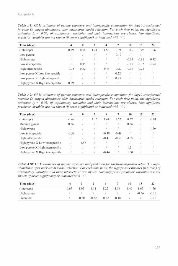
Appendix A
134
Table A8: GLM estimates of pyrene exposure and interspecific competition for log10-transformed juvenile D. magna abundance after backwards model selection. For each time point, the significant estimates (p < 0.05) of explanatory variables and their interactions are shown. Non-significant predictor variables are not shown (if never significant) or indicated with “/”.
Time (days) -4 0 2 4 7 10 15 22 (Intercept) 0.79 0.56 1.21 1.56 1.89 1.83 1.59 1.06 Low pyrene / / / / -0.17 / / / High pyrene / / / / / -0.14 -0.81 0.42 Low interspecific / 0.35 / / / -0.15 -0.32 -0.42 High interspecific -0.35 0.32 / -0.14 -0.27 -0.16 -0.23 / Low pyrene X Low interspecific / / / / 0.22 / / / Low pyrene X High interspecific / / / / 0.23 / / / High pyrene X High interspecific 0.59 / / / / / / /
Table A9: GLM estimates of pyrene exposure and interspecific competition for log10-transformed neonate D. magna abundance after backwards model selection. For each time point, the significant estimates (p < 0.05) of explanatory variables and their interactions are shown. Non-significant predictor variables are not shown (if never significant) or indicated with “/”.
Time (days) -4 0 2 4 7 10 15 22 (Intercept) -0.48 / 1.15 1.44 1.52 0.57 / -0.81 Medium pyrene 0.56 / / / / 0.56 / / High pyrene / / / / / / / 1.79 Low interspecific -0.59 / / -0.38 -0.49 / / / High interspecific / / / -0.41 -0.57 -1.22 / / High pyrene X Low interspecific / -1.58 / / / / / / Low pyrene X High interspecific / / / / / 1.21 / / High pyrene X High interspecific / / / -0.44 / 1.00 / /
Table A10: GLM estimates of pyrene exposure and predation for log10-transformed adult D. magna abundance after backwards model selection. For each time point, the significant estimates (p < 0.05) of explanatory variables and their interactions are shown. Non-significant predictor variables are not shown (if never significant) or indicated with “/”.
Time (days) -4 0 2 4 7 10 15 22 (Intercept) 0.67 1.02 1.11 1.22 1.36 1.49 1.67 1.76 High pyrene / / / / / / -0.36 -0.16 Predation / -0.20 -0.22 -0.22 -0.18 / / -0.16

Supportive Information Chapter 2
135
Table A11: GLM estimates of pyrene exposure and predation for log10-transformed juvenile D. magna abundance after backwards model selection. For each time point, the significant estimates (p < 0.05) of explanatory variables and their interactions are shown. Non-significant predictor variables are not shown (if never significant) or indicated with “/”.
Time (days) -4 0 2 4 7 10 15 22 (Intercept) 0.67 0.55 1.01 1.56 1.89 1.79 1.56 1.27 Medium pyrene / / / / -0.28 / / / High pyrene / / / / / / -0.70 / Predation / / / -0.34 -0.36 -0.37 -0.50 -0.33
Table A12: GLM estimates of pyrene exposure and predation for log10-transformed neonate D. magna abundance after backwards model selection. For each time point, the significant estimates (p < 0.05) of explanatory variables and their interactions are shown. Non-significant predictor variables are not shown (if never significant) or indicated with “/”.
Time (days) -4 0 2 4 7 10 15 22 (Intercept) / / 1.25 1.51 1.47 0.57 -0.42 -0.57 High pyrene / 0.79 / / / / / 0.96 Predation / / -0.67 -1.03 -0.80 / / / Low pyrene X Predation / / / / / -1.07 / /

Appendix A
136
Figure A1. Optimal concentration response curve for pyrene fitted to the results of a 48 hours test with neonate D. magna.
Figure A2. Adult D. magna abundance over time for four pyrene exposure profiles: control, low, medium and high pyrene exposure. Data shown are the adult D. magna abundances with no additional species interactions. Average values with standard deviations (error bars) are depicted. Dashed lines indicate the first and the second pyrene application.

Supportive Information Chapter 2
137
Figure A3. Adult D. magna abundance over time for four pyrene exposure profiles: control, low, medium and high pyrene exposure. Data shown are the treatments without (points) and with predation (crosses). Average values with standard deviations (error bars) are depicted. Dashed lines indicate the first and the second pyrene application.
Figure A4. Adult D. magna abundance over time for four pyrene exposure profiles: control, low, medium and high pyrene exposure. Data shown are the treatments with no additional species interactions (points), low intraspecific competition (crosses) and high intraspecific competition (black squares). Average values with standard deviations (error bars) are depicted. Dashed lines indicate the first and the second pyrene application.

Appendix A
138
Figure A5. Adult D. magna abundance over time for four pyrene exposure profiles: control, low, medium and high pyrene exposure. Data shown are the treatments with no additional species interactions (points), low interspecific competition (crosses) and high interspecific competition (black squares). Average values with standard deviations (error bars) are depicted. Dashed lines indicate the first and the second pyrene application.
Figure A6. Juvenile D. magna abundance over time for four pyrene exposure profiles: control, low, medium and high pyrene exposure. Data shown are the juvenile D. magna abundances with no additional species interactions. Average values with standard deviations (error bars) are depicted. Dashed lines indicate the first and the second pyrene application.

Supportive Information Chapter 2
139
Figure A7. Juvenile D. magna abundance over time for four pyrene exposure profiles: control, low, medium and high pyrene exposure. Data shown are the treatments without (points) and with predation (crosses). Average values with standard deviations (error bars) are depicted. Dashed lines indicate the first and the second pyrene application.
Figure A8. Juvenile D. magna abundance over time for four pyrene exposure profiles: control, low, medium and high pyrene exposure. Data shown are the treatments with no additional species interactions (points), low intraspecific competition (crosses) and high intraspecific competition (black squares). Average values with standard deviations (error bars) are depicted. Dashed lines indicate the first and the second pyrene application.

Appendix A
140
Figure A9. Juvenile D. magna abundance over time for four pyrene exposure profiles: control, low, medium and high pyrene exposure. Data shown are the treatments with no additional species interactions (points), low interspecific competition (crosses) and high interspecific competition (black squares). Average values with standard deviations (error bars) are depicted. Dashed lines indicate the first and the second pyrene application.
Figure A10. Neonate D. magna abundance over time for four pyrene exposure profiles: control, low, medium and high pyrene exposure. Data shown are the neonate D. magna abundances with no additional species interactions. Average values with standard deviations (error bars) are depicted. Dashed lines indicate the first and the second pyrene application.

Supportive Information Chapter 2
141
Figure A11. Neonate D. magna abundance over time for four pyrene exposure profiles: control, low, medium and high pyrene exposure. Data shown are the treatments without (points) and with predation (crosses). Average values with standard deviations (error bars) are depicted. Dashed lines indicate the first and the second pyrene application.
Figure A12. Neonate D. magna abundance over time for four pyrene exposure profiles: control, low, medium and high pyrene exposure. Data shown are the treatments with no additional species interactions (points), low intraspecific competition (crosses) and high intraspecific competition (black squares). Average values with standard deviations (error bars) are depicted. Dashed lines indicate the first and the second pyrene application.
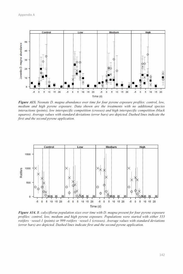
Appendix A
142
Figure A13. Neonate D. magna abundance over time for four pyrene exposure profiles: control, low, medium and high pyrene exposure. Data shown are the treatments with no additional species interactions (points), low interspecific competition (crosses) and high interspecific competition (black squares). Average values with standard deviations (error bars) are depicted. Dashed lines indicate the first and the second pyrene application.
Figure A14. B. calyciflorus population sizes over time with D. magna present for four pyrene exposure profiles: control, low, medium and high pyrene exposure. Populations were started with either 333 rotifers · vessel-1 (points) or 999 rotifers · vessel-1 (crosses). Average values with standard deviations (error bars) are depicted. Dashed lines indicate first and the second pyrene application.
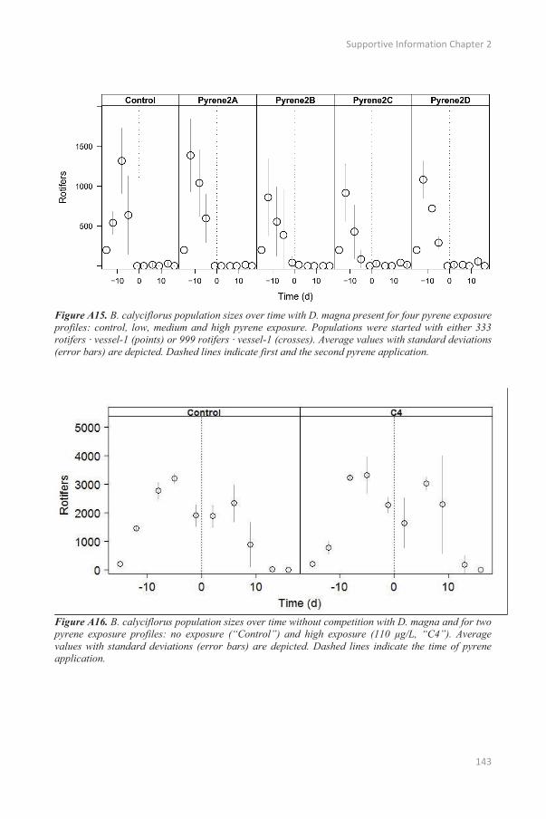
Supportive Information Chapter 2
143
Figure A15. B. calyciflorus population sizes over time with D. magna present for four pyrene exposure profiles: control, low, medium and high pyrene exposure. Populations were started with either 333 rotifers · vessel-1 (points) or 999 rotifers · vessel-1 (crosses). Average values with standard deviations (error bars) are depicted. Dashed lines indicate first and the second pyrene application.
Figure A16. B. calyciflorus population sizes over time without competition with D. magna and for two pyrene exposure profiles: no exposure (“Control”) and high exposure (110 μg/L, “C4”). Average values with standard deviations (error bars) are depicted. Dashed lines indicate the time of pyrene application.


145
B SUPPORTIVE INFORMATION CHAPTER 4

Appendix B
146
Figure B1: Likelihood (LSS) of the DEBkiss models with values for the maximum area-specific assimilation rate (max_spec_assimr) between 0.006 and 0.121 mg mm-2 d-1.

Supportive Information Chapter 4
147
Figure B2: Total population density (A) and densities of large (B), medium (C) and small (D)
individuals for D. magna using a DEBkiss IBM without additional food starvation mortality. Black
bullets and squares show the observed dynamics for populations without additional stress in two
experiments. Green areas show the best predictions.
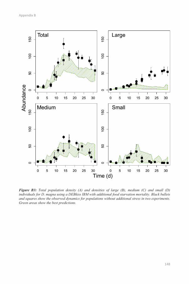
Appendix B
148
Figure B3: Total population density (A) and densities of large (B), medium (C) and small (D) individuals for D. magna using a DEBkiss IBM with additional food starvation mortality. Black bullets and squares show the observed dynamics for populations without additional stress in two experiments. Green areas show the best predictions.

149
C SUPPORTIVE INFORMATION CHAPTER 5

Appendix C
150
C.1. Literature sources for DEBkiss parameters
Asellus: (Maltby 1991, 1995; Arakelova 2001; Galic et al. 2012)
Brachionus: (Halbach 1970a; Dumont et al. 1975; Saunders III and Lewis Jr 1988; Hansen and Bjornsen
1997; Mohr and Adrian 2000; Jensen and Verschoor 2004)
Chaoborus: (Stenson 1978; Van Wijngaarden et al. 2006)
Daphnia: (MacArthur and Baillie 1929; Dumont et al. 1975; Tillmann and Lampert 1984; Ebert 1992;
Glazier 1992; Trubetskova and Lampert 1995; Jager and Zimmer 2012; Mulder and Hendriks
2014)
Gammarus: (Nilsson 1977; Welton and Clarke 1980; Gee 1988; Ward 1988; McCahon and Pascoe
1990; Maltby 1995)
C.2. Derivation of multi-species predation equation
Disc equation for multiple prey:
(Rose et al 1999)
Where Cj = the biomass of prey j eaten by predator I (g); Cmax = the maximum food uptake by predator
i (g d-1); Wi = the weight of the predator i (g); PDj = the density of prey j (prey L-1); Kj = the half-
saturation coefficient for prey j (prey L-1); n = the numer of prey species for predator i.
Data available for Daphnia and Brachionus are based on:
′
′ (Krylov 1992)
Where PR = predation rate (prey predator-1 d-1); a’j = attack rate on prey j (L d-1); Nj = density of prey j
(prey L-1); Thj = handling time of prey j (d); n = the number of prey species.
To implement multi-species predation in the IBMs, we need the biomass of prey eaten. However, we
only have the parameters for the Krylov 1992 equation. Therefore, we combine both equations using the
half-saturation coefficient K. The half-saturation coefficient K in a type II functional response function
corresponds with the food density at which the food uptake is exactly 50% of the maximum food uptake.
For the Krylov 1992 equation, the maximum food uptake corresponds to the limit of the function i.e.
. Therefore the Krylov 1992 equivalent of K is equal to . The corresponding food density N is
calculated by:
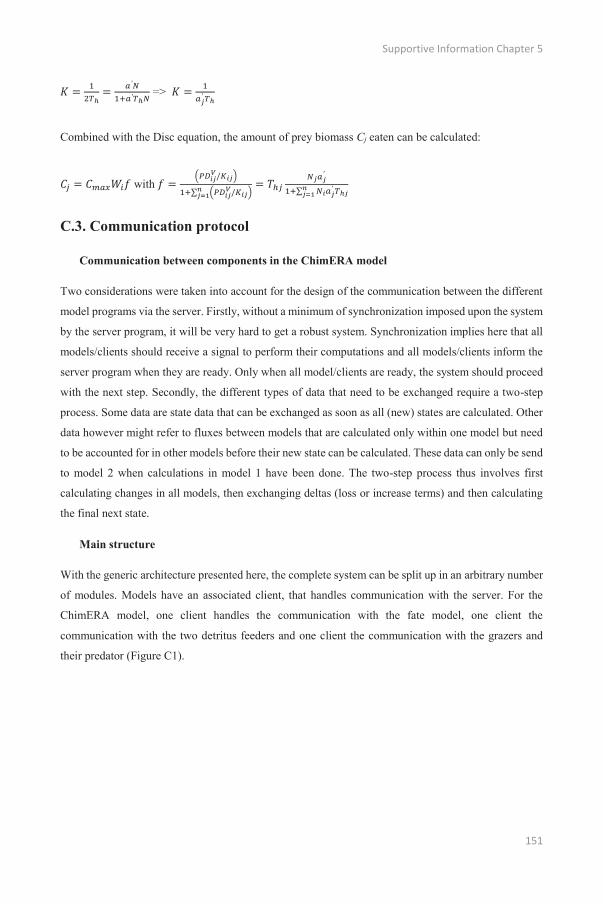
Supportive Information Chapter 5
151
′
′ => ′
Combined with the Disc equation, the amount of prey biomass Cj eaten can be calculated:
with ′
′
C.3. Communication protocol
Communication between components in the ChimERA model
Two considerations were taken into account for the design of the communication between the different
model programs via the server. Firstly, without a minimum of synchronization imposed upon the system
by the server program, it will be very hard to get a robust system. Synchronization implies here that all
models/clients should receive a signal to perform their computations and all models/clients inform the
server program when they are ready. Only when all model/clients are ready, the system should proceed
with the next step. Secondly, the different types of data that need to be exchanged require a two-step
process. Some data are state data that can be exchanged as soon as all (new) states are calculated. Other
data however might refer to fluxes between models that are calculated only within one model but need
to be accounted for in other models before their new state can be calculated. These data can only be send
to model 2 when calculations in model 1 have been done. The two-step process thus involves first
calculating changes in all models, then exchanging deltas (loss or increase terms) and then calculating
the final next state.
Main structure
With the generic architecture presented here, the complete system can be split up in an arbitrary number
of modules. Models have an associated client, that handles communication with the server. For the
ChimERA model, one client handles the communication with the fate model, one client the
communication with the two detritus feeders and one client the communication with the grazers and
their predator (Figure C1).
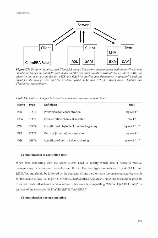
Appendix C
152
Figure C1: Setup of the integrated ChimERA model. The server communicates with three clients. One client coordinates the chimERA fate model and the two other clients coordinate the DEBkiss IBMs: one client for the two detritus feeders (ASE and GAM for Asellus and Gammarus, respectively) and one client for the two grazers and the predator (BRA. DAP and CHA for Brachionus, Daphnia and Chaoborus, respectively).
Table C1: Data exchanged between the communication server and clients.
Name Type Definition Unit
PHY STATE Phytoplankton concentration mg ww L-1
CPW STATE Concentration chemical in water mol L-1
PGL DELTA Loss (flux) of phytoplankton due to grazing mg ww L-1 h-1
DET STATE Detritus (in water) concentration mg ww L-1
DGL DELTA Loss (flux) of detritus due to grazing mg ww L-1 h-1
Communication at connection time
When first connecting with the sever, clients need to specify which data it needs to receive,
distinguishing between state variables and fluxes. The two types are indicated by &STATE and
&DELTA, and should be followed by the character @ and zero or more (comma-separated) keywords
for the data, e.g., '&STATE@PHY,ZOOP1,ZOOP2&DELTA@GRA*'. Note that it should be possible
to include models that do not need input from other models, so signalling: '&STATE@&DELTA@*' or
just one of the two types: '&STATE@&DELTA@GRA*'
Communication during simulation

Supportive Information Chapter 5
153
The basic loop for each time step is worked out below. The following synchronized steps occur, starting
at the moment all models’ state variables have just been updated. Exclamation marks are used to indicate
the start of a command given by the server, or the following reply coming from the client.
1. Server sends: !calcDelta* to all (waiting) clients and waits for replies from all. No data accompanies
this command. The client allows its model to run up to the moment the next/new state is calculated.
It has to stop then, because the calculation of the final new state may require information exchange
with other models.
2. All clients send: !delta* to the server, to signal that they are ready. When a client produced
information that is needed in other models, the standard data string (possibly composed) with this
information should be appended to !delta, e.g. !delta#1&GRA@1,2,3,4,5,6,7,8,9,10*. After sending
confirmation/data, clients wait.
3. When all confirmations have arrived at the server, the server starts the exchange of delta data by
building for all clients that expressed the need for these data, the pure (and possibly composed) delta
data strings, and subsequently sending them. The information from the server has the format
!delta<data-string>*, with data-string in the format we decided upon, e.g.
!delta#1&PGL@1,2,3,4,5,6,7,8,9,10&DGL@9,8,7,6,5,4,3,2,1,0* or
!delta#1&PGL@1,2,3,4,5,6,7,8,9,10*. In the data string, any arbitrary data can be included. These
data – not needed by other models – will not be exchanged between component models, but only
stored and visualized by the server. E.g.,
!delta#1&PGL@1,2,3,4,5,6,7,8,9,10&MYDATA@9,8,7,6,5,4,3,2,1,0*.
4. Server waits until all the clients that needed delta data have signalled that these data have been
received, e.g. by replying !received*
5. All clients now wait until the server sends them the message !calcState*. Upon receiving this
message the clients make their model do the necessary thing to set the new state of the model (e.g.
subtracting or adding fluxes calculated in other compartments/models).
6. When new state has been set in the models, all clients have to signal that they are ready, by sending
!state* to the server. In case clients provide state data that are needing in other models, the (possibly
composed) state data are appended: !state<data-string>* e.g. !state#1&PHY@1,2,3,4,5,6,7,8,9,10*.
After sending confirmation, clients wait. Also here, in the data string, any arbitrary data can be
included. These data – not needed by other models – will not be exchanged between component
models, but only stored and visualized by the server. E.g.,
!state#1&PHY@1,2,3,4,5,6,7,8,9,10&MYDATA@9,8,7,6,5,4,3,2,1,0*.
7. When all these confirmations have arrived at the server, the server starts the exchange of state data
by building for all clients that expressed the need for these data, the pure (and possibly composed)
state data strings, and subsequently sending them.

Appendix C
154
8. Server waits until all the clients that needed state data have signalled that these data have been
received, e.g. by replying !received*
9. Etc. continuing with step 1. This is the moment the server might be interrupted, leaving the system
in a resumable state.
Some specials steps need to be taken when initializing the whole system. Initialization can be done by
a variant of the steps 5 to 8 (related to setting state):
10. After the connections have been made (open socket connection created between server and client)
all clients wait until the server sends them the message !initialize*. Upon receiving this message the
clients make their model do the necessary initializations to set the state of the model at time 0 (this
refers to state that can be initialized without information on the initial state of other models).
11. When initializations are done in the models, all clients have to signal that they are ready, by sending
!initialized* to the server. In case clients provide state data that are needed in other models, the
(possibly composed) state data are appended, e.g., !initialized#1&PHY@1,2,3,4,5,6,7,8,9,10*.
After sending confirmation, clients wait. (we could also just copy/reuse the !state* protocol).
12. When all these confirmations have arrived at the server, the server starts the exchange of state data
by building for all clients that expressed the need for these data, the pure (and possibly composed)
state data strings, and subsequently sending them.
13. Server waits until all the clients that needed state data have signalled that these data have been
received, e.g. by replying !received*. After this, all models have their complete up to date state
related to t = 0.

155
D SUPPORTIVE INFORMATION CHAPTER 6
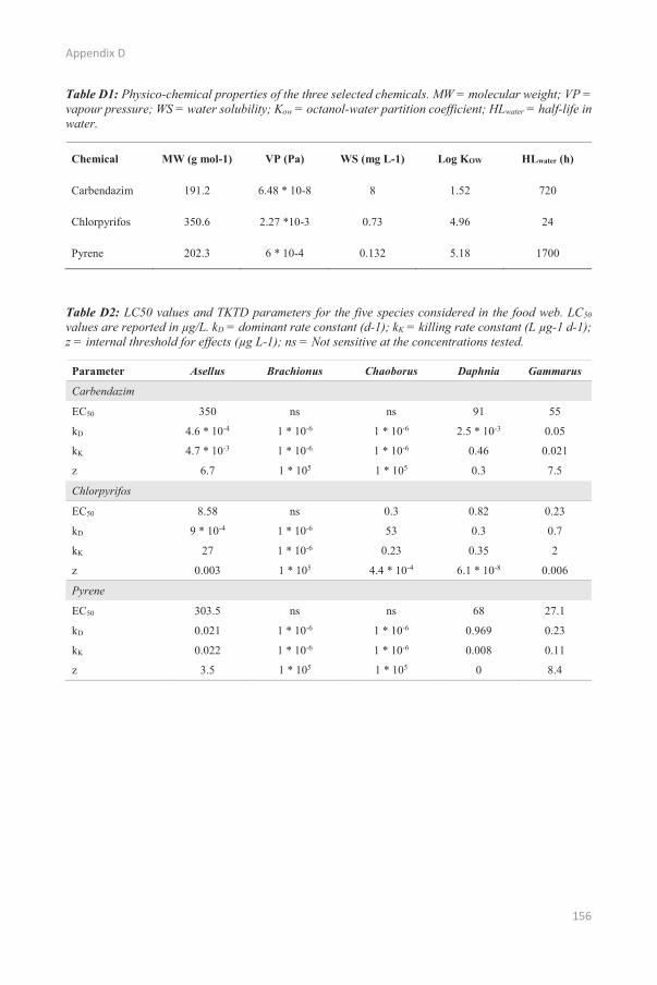
Appendix D
156
Table D1: Physico-chemical properties of the three selected chemicals. MW = molecular weight; VP = vapour pressure; WS = water solubility; Kow = octanol-water partition coefficient; HLwater = half-life in water.
Chemical MW (g mol-1) VP (Pa) WS (mg L-1) Log KOW HLwater (h)
Carbendazim 191.2 6.48 * 10-8 8 1.52 720
Chlorpyrifos 350.6 2.27 *10-3 0.73 4.96 24
Pyrene 202.3 6 * 10-4 0.132 5.18 1700
Table D2: LC50 values and TKTD parameters for the five species considered in the food web. LC50 values are reported in μg/L. kD = dominant rate constant (d-1); kK = killing rate constant (L μg-1 d-1); z = internal threshold for effects (μg L-1); ns = Not sensitive at the concentrations tested.
Parameter Asellus Brachionus Chaoborus Daphnia Gammarus
Carbendazim
EC50 350 ns ns 91 55
kD 4.6 * 10-4 1 * 10-6 1 * 10-6 2.5 * 10-3 0.05
kK 4.7 * 10-3 1 * 10-6 1 * 10-6 0.46 0.021
z 6.7 1 * 105 1 * 105 0.3 7.5
Chlorpyrifos
EC50 8.58 ns 0.3 0.82 0.23
kD 9 * 10-4 1 * 10-6 53 0.3 0.7
kK 27 1 * 10-6 0.23 0.35 2
z 0.003 1 * 105 4.4 * 10-4 6.1 * 10-8 0.006
Pyrene
EC50 303.5 ns ns 68 27.1
kD 0.021 1 * 10-6 1 * 10-6 0.969 0.23
kK 0.022 1 * 10-6 1 * 10-6 0.008 0.11
z 3.5 1 * 105 1 * 105 0 8.4

157
REFERENCES
References
158
Abbriano RM, Carranza MM, Hogle SL, Levin RA, Netburn AN, Seto KL, et al. Deepwater Horizon Oil Spill: A Review of the Planktonic Response. Oceanography. 2011;24(3):294–301.
Adams J, Gee J, Greenwood P, McKelvey S, Perry R. Factors affecting the microdistribution of Gammarus pulex (Amphipoda): an experimental study. Freshw Biol. 1987;17(2):307–16.
Arakelova KS. The evaluation of individual production and scope for growth in aquatic sow bugs (Asellus aquaticus). Aquat Ecol. 2001;35(1):31–42.
Augusiak J, Van den Brink PJ, Grimm V. Merging validation and evaluation of ecological models to “evaludation”: A review of terminology and a practical approach. Ecol Modell. 2014;280:117–28.
Baird DJ, Barber I, Bradley M, Soares AMVM, Calow P. A comparative study of genotype sensitivity to acute toxic stress using clones of Daphnia magna straus. Ecotoxicol Environ Saf. 1991;21(3):257–65.
Baird DJ, Maltby LL, Greig-Smith PW, Douben PET. ECOtoxicology: Ecological dimensions. Chapman & Hall Ecotoxicology Series; 1996.
Beketov M a, Liess M. The influence of predation on the chronic response of Artemia sp. populations to a toxicant. J Appl Ecol. 2006;43(6):1069–74.
Beketov MA, Liess M. Ecotoxicology and macroecology - Time for integration. Environ Pollut. 2012;162:247–54.
Bellas J, Saco-Alvarez L, Nieto O, Beiras R. Ecotoxicological evaluation of polycyclic aromatic hydrocarbons using marine invertebrate embryo-larval bioassays. Mar Pollut Bull. 2008;57(6-12):493–502.
Bontje D, Kooi BW, Liebig M, Kooijman SALM. Modelling long-term ecotoxicological effects on an algal population under dynamic nutrient stress. Water Res. 2009;43(13):3292–300.
Bradbury SP, Feijtel TCJ, Van Leeuwen CJ. Meeting the scientific needs of ecological risk assessment in a regulatory context. Environ Sci Technol. 2004;38(23):463a – 470a.
Bray JR, Curtis JT. An Ordination of the upland forest community of southern Wisconsin.pdf. Ecol Monogr. 1957;27(4):325–49.
Bridges CM. Long-term effects of pesticide exposure at various life stages of the southern leopard frog (Rana sphenocephala). Arch Environ Contam Toxicol. 2000;39(1):91–6.
Brock TCM, Arts GHP, Maltby L, Van den Brink PJ, Maltby ÀL, Brink PJ Van Den. Aquatic risks of pesticides, ecological protection goals, and common aims in european union legislation. Integr Environ Assess Manag. 2006;2(4):e20–46.
Brock TCM, Roessink I, Belgers JDM, Bransen F, Maund SJ. Impact of a Benzoyl Urea Insecticide on Aquatic Macroinvertebrates in Ditch Mesocosms with and without Non-Sprayed Sections. Environ Toxicol Chem. 2009;28(10):2191–205.
Cairns J. Putting the eco in ecotoxicology. Regul Toxicol Pharmacol. 1988;8(2):226–38.
Caquet T, Deydier-Stephan L, Lacroix G, Le Rouzic B, Lescher-Moutoue F. Effects of fomesafen, alone and in combination with an adjuvant, on plankton communities in freshwater outdoor pond mesocosms. Environ Toxicol Chem. 2005;24(5):1116–24.
Cardinale BJ, Duffy JE, Gonzalez A, Hooper DU, Perrings C, Venail P, et al. Biodiversity loss and its impact on humanity. Nature. 2012;486(7401):59–67.

References
159
Chapman PM, Fairbrother A, Brown D. A critical evaluation of safety (uncertainty) factors for ecological risk assessment. Environ Toxicol Chem. 1998;17(1):99–108.
Chapman PM. Integrating toxicology and ecology: putting the “eco” into ecotoxicology. Mar Pollut Bull. 2002;44(1):7–15.
Chuvieco E, Aguado I, Yebra M, Nieto H, Salas J, Martín MP, et al. Development of a framework for fire risk assessment using remote sensing and geographic information system technologies. Ecol Modell. 2010;221(1):46–58.
Clements WH, Rohr JR. Community responses to contaminants: Using basic ecological principles to predict ecotoxicological effects. Environ Toxicol Chem. 2009;28(9):1789–800.
Coors A, Meester L De. Synergistic, antagonistic and additive effects of multiple stressors: predation threat, parasitism and pesticide exposure in Daphnia magna. J Appl Ecol. 2008;45:1820–8.
Daam MA, Van den Brink PJ. Implications of differences between temperate and tropical freshwater ecosystems for the ecological risk assessment of pesticides. Ecotoxicology. 2010;19(1):24–37.
Day KE, Kaushik NK, Solomon KR. Impact of Fenvalerate on Enclosed Freshwater Planktonic Communities and on in situ Rates of Filtration of Zooplankton. Can J Fish Aquat Sci. 1987;44(10):1714–28.
De Hoop L, De Troch M, Hendriks a J, De Laender F. Modeling toxic stress by atrazine in a marine consumer-resource system. Environ Toxicol Chem. 2013;32(5):1088–95.
De Laender F, De Schamphelaere KAC, Vanrolleghem P a, Janssen CR. Is ecosystem structure the target of concern in ecological effect assessments? Water Res. 2008a;42(10-11):2395–402.
De Laender F, De Schamphelaere KAC, Vanrolleghem P a, Janssen CR. Validation of an ecosystem modelling approach as a tool for ecological effect assessments. Chemosphere. 2008b;71(3):529–45.
De Laender F, De Schamphelaere KAC, Vanrolleghem PA, Janssen CR. Do we have to incorporate ecological interactions in the sensitivity assessment of ecosystems? An examination of a theoretical assumption underlying species sensitivity distribution models. Environ Int. 2008c;34(3):390–6.
De Laender F, Janssen CR. The ecosystem perspective in ecotoxicology as a way forward for the ecological risk assessment of chemicals. Integr Environ Assess Manag. 2013;9(3):e34–8.
De Laender F, Melian CJ, Bindler R, Van den Brink PJ, Daam M, Roussel H, et al. The contribution of intra- and interspecific tolerance variability to biodiversity changes along toxicity gradients. Ecol Lett. 2014b;17(1):72–81.
De Laender F, Morselli M, Baveco H, Van den Brink PJ, Di Guardo A. Theoretically exploring direct and indirect chemical effects across ecological and exposure scenarios using mechanistic fate and effects modelling. Environ Int. 2015;74:181–90.
De Laender F, Taub FB, Janssen CR. Ecosystem functions and densities of contributing functional groups respond in a different way to chemical stress. Environ Toxicol Chem. 2011;30(12).
De Laender F, van den Brink PJ, Janssen CR, Di Guardo A. The ChimERA project: Coupling mechanistic exposure and effect models into an integrated platform for ecological risk assessment. Environ Sci Pollut Res. 2014a;21:6263–7.
De Laender F, Van Sprang P, Janssen CR. A re-evaluation of fifteen years of european risk assessment using effect models. Environ Toxicol Chem. 2013;32(3):594–601.

References
160
De Lange HJ, Sala S, Vighi M, Faber JH. Ecological vulnerability in risk assessment - A review and perspectives. Sci Total Environ. 2010;408(18):3871–9.
Del Arco AI, Parra G, Rico A, Van den Brink PJ. Effects of intra- and interspecific competition on the sensitivity of aquatic macroinvertebrates to carbendazim. Ecotoxicol Environ Saf. 2015;120:27–34.
Deneer JW. Toxicity of mixtures of pesticides in aquatic systems. Pest Manag Sci. 2000 Jun;56(6):516–20.
Di Guardo A, Morselli M, Morabito G, Van den Brink PJ, De Laender F. European-wide ecological scenarios for the exposure assessment of chemicals in aquatic systems. Prep.
Di Toro DM, McGrath JA, Hansen DJ. Technical basis for narcotic chemicals and polycyclic aromatic hydrocarbon criteria. I. Water and Tissue. Environ Toxicol Chem. 2000;19(8):1951–70.
Dohmen GP, Preuss TG, Hamer M, Galic N, Strauss T, Van den Brink PJ, et al. Population-level effects and recovery of aquatic invertebrates after multiple applications of an insecticide. Integr Environ Assess Manag. 2015;9999(9999):1–15.
Dom N, Penninck M, Knapen D, Blust R. Discrepancies in the acute versus chronic toxicity of compounds with a designated narcotic mechanism. Chemosphere. 2012;87(7):742–9.
Dumbauld BR, Brooks KM, Posey MH. Response of an estuarine benthic community to application of the pesticide carbaryl and cultivation of Pacific oysters (Crassostrea gigas) in Willapa Bay, Washington. Mar Pollut Bull. 2001;42(10):826–44.
Dumont HJ, Balvay G. The dry weight estimate of Chaoborus flavicans (Meigen) as a function of length and instars. Hydro. 1979;64(2):139–45.
Dumont HJ, Velde I, Dumont S. The dry weight estimate of biomass in a selection of Cladocera, Copepoda and Rotifera from the plankton, periphyton and benthos of continental waters. Oecologia. 1975;19(1):75–97.
Ebert D. A food-independent maturation treshold and size at maturity in Daphnia magna. Limnol Oceanogr. 1992;37(4):878–81.
EC. Council Directive 91/414/EEC of 15 July 1991 concerning the placing of plant protection products on the market. Consolidated text including amendments. 2004;
EC. Directive 2000/60/EC of the European parliament and of the council of 23 October 2000 establishing a framework for Community action in the field of water policy. Official J Eur Communities. 2000;L327:1–72.
EC. Regulation (EC) No 1907/2006 of the European Parliament and of the Council of 18 December 2006 concerning the Registration, Evaluation, Authorisation and Restriction of Chemicals (REACH), establishing a European Chemicals Agency, amending Directive 1999/4. Official J Eur Communities. 2007;L136(3).
Fleeger JW, Carman KR, Nisbet RM. Indirect effects of contaminants in aquatic ecosystems. Sci Total Environ. 2003;317(1-3):207–33.
FOCUS. FOCUS surface water scenarios in the EU evaluation process under 91/414/EEC; rev. 2. FOCUS Working Group on Surface Water Scenarios (EC Document Reference SANCO/4802/2001). 2001;245.
Foit K, Kaske O, Liess M. Competition increases toxicant sensitivity and delays the recovery of two interacting populations. Aquat Toxicol. 2012;106-107:25–31.
References
161
Forbes VE, Calow P, Grimm V, Hayashi T, Jager T, Palmqvist A, et al. Integrating population modeling into ecological risk assessment. Integr Environ Assess Manag. 2009a;6(1):191–3.
Forbes VE, Calow P, Sibly RM. Are current species extrapolation models a good basis for ecological risk assessment? Environ Toxicol Chem. 2001;20(2):442–7.
Forbes VE, Calow P, Sibly RM. The extrapolation problem and how population modeling can help. Environ Toxicol Chem. 2008;27(10):1987–94.
Forbes VE, Calow P. Promises and problems for the new paradigm for risk assessment and an alternative approach involving predictive systems models. Environ Toxicol Chem. 2012;31(12):2663–71.
Forbes VE, Calow P. Species sensitivity distributions revisited: A critical appraisal. Hum Ecol Risk Assess. 2002;8(3):473–92.
Forbes VE, Hommen U, Thorbek P, Heimbach F, Van den Brink PJ, Wogram J, et al. Ecological models in support of regulatory risk assessments of pesticides: developing a strategy for the future. Integr Environ Assess Manag. 2009b;5(1):167–72.
Gabsi F, Hammers-Wirtz M, Grimm V, Schäffer A, Preuss TG. Coupling different mechanistic effect models for capturing individual- and population-level effects of chemicals: Lessons from a case where standard risk assessment failed. Ecol Modell. 2014a;280:18–29.
Gabsi F, Schäffer A, Preuss TG. Predicting the sensitivity of populations from individual exposure to chemicals: the role of ecological interactions. Environ Toxicol Chem. 2014b;33(7):1449–57.
Galic N, Ashauer R, Baveco H, Nyman AM, Barsi A, Thorbek P, et al. Modelling the contribution of toxicokinetic and toxicodynamic processes to the recovery of Gammarus pulex populations after exposure to pesticides. Environ Toxicol Chem. 2014;33(7):1476–88.
Galic N, Baveco H, Hengeveld GM, Thorbek P, Bruns E, van den Brink PJ. Simulating population recovery of an aquatic isopod: Effects of timing of stress and landscape structure. Environ Pollut. 2012;163:91–9.
Galic N, Hommen U, Baveco JMH, van den Brink PJ. Potential application of population models in the European ecological risk assessment of chemicals. II. Review of models and their potential to address environmental protection aims. Integr Environ Assess Manag. 2010;6(3):338–60.
Gama-Flores JL, Sarma SSS, Nandini S. Effect of cadmium level and exposure time on the competition between zooplankton species Moina macrocopa (Cladocera) and Brachionus calyciflorus (Rotifera). J Environ Sci Health A Tox Hazard Subst Environ Eng. 2006;41(6):1057–70.
Gee JHR. Population dynamics and morphometries of Gammarus pulex L.: evidence of seasonal food limitation in a freshwater detritivore. Freshw Biol. 1988;19:333–43.
Gergs A, Zenker A, Grimm V, Preuss TG. Chemical and natural stressors combined: from cryptic effects to population extinction. Sci Rep. 2013;3(2036).
Gilbert JJ. Competition between Rotifers and Daphnia. Ecology. 1985;66(6):1943–50.
Gilbert JJ. Suppression of rotifer populations by Daphnia: A review of the evidence, the mechanisms, and the effects on zooplankton community structure. Limnol Oceanogr. 1988;33(6):1286–303.
Girling AE, Pascoe D, Janssen CR, Peither A, Wenzel A, Schafer H, et al. Development of methods for evaluating toxicity to freshwater ecosystems. Ecotoxicol Environ Saf. 2000;45(2):148–76.
Glazier DS. Effects of Food, Genotype, and Maternal Size and Age on Offspring Investment in Daphnia Magna. Ecology. 1992;73(3):910–26.

References
162
Grimm V, Ashauer R, Forbes V, Hommen U, Preuss TG, Schmidt A, et al. CREAM: a European project on mechanistic effect models for ecological risk assessment of chemicals. Environ Sci Pollut Res Int. 2009;16(6):614–7.
Grimm V, Berger U, Bastiansen F, Eliassen S, Ginot V, Giske J, et al. A standard protocol for describing individual-based and agent-based models. Ecol Modell. 2006;198(1-2):115–26.
Grimm V, Martin BT. Mechanistic effect modeling for ecological risk assessment: Where to go from here? Integr Environ Assess Manag. 2013;9(3):e58–63.
Grimm V, Railsback SF. Individual-based Modeling and Ecology. Princeton University Press; 2013.
Grimm V, Thorbek P. Population models for ecological risk assessment of chemicals: Short introduction and summary of a special issue. Ecol Modell. 2014;280:1–4.
Gunderson AR, Armstrong EJ, Stillman JH. Multiple Stressors in a Changing World: The Need for an Improved Perspective on Physiological Responses to the Dynamic Marine Environment. Ann Rev Mar Sci. 2016;8(1):13–41.
Håkanson L, Peters RH. Predictive Limnology: Methods for Predictive Modelling. Amsterdam: SPB Academic Publishing bv.; 1995.
Halbach U. Die Ursachen der Temporalvariation yon Brachionus calyciflorus Pallas (Rotatoria ). Oecologia. 1970a;4:262–318.
Halbach U. EinfluB der Temperatur auf die Populationsdynamik des planktischen Rädertieres Brachionus calyciflorus Pallas. Oecologia. 1970b;207:176–207.
Hanazato T. Pesticide effects on freshwater zooplankton : an ecological perspective. Environ Pollut. 2001;112:1–10.
Hansen PJ, Bjornsen PK. Zooplankton grazing and growth: Scaling within the 2-2,000-mu m body size range. Limnol Oceanogr. 1997;42(4):687–704.
Hjorth M, Vester J, Henriksen P, Forbes V, Dahllöf I. Functional and structural responses of marine plankton food web to pyrene contamination. Mar Ecol Prog Ser. 2007;338:21–31.
Hoang TC, Klaine SJ. Influence of organism age on metal toxicity to Daphnia magna. Environ Toxicol Chem. 2007;26(6):1198–204.
Hommen U, Baveco JM, Galic N, van den Brink PJ. Potential Application of Ecological Models in the European Environmental Risk Assessment of Chemicals I: Review of Protection Goals in EU Directives and Regulations. Integr Environ Assess Manag. 2010;6(3):325–37.
Hommen U, Forbes V, Grimm V, Preuss TG, Thorbek P, Ducrot V. How to use mechanistic effect models in environmental risk assessment of pesticides: Case studies and recommendations from the SETAC workshop MODELINK. Integr Environ Assess Manag. 2016;12(1):21–31.
Hooper DU, Adair EC, Cardinale BJ, Byrnes JEK, Hungate BA, Matulich KL, et al. A global synthesis reveals biodiversity loss as a major driver of ecosystem change. Nature. 2012;486:105–8.
Hooper DU, Chapin FS, Ewel JJ, Hector A, Inchausti P, Lavorel S, et al. Effects of Biodiversity on Ecosystem Functioning: a Consensus of Current Knowledge. Ecol Monogr. 2005;75(1):3–35.
Hose GC, Van den Brink PJ. Confirming the species-sensitivity distribution concept for endosulfan using laboratory, mesocosm, and field data. Arch Environ Contam Toxicol. 2004;47(4):511–20.
References
163
Jager T, Albert C, Preuss TG, Ashauer R. General Unified Threshold Model of Survival - a Toxicokinetic-Toxicodynamic Framework for Ecotoxicology. Environ Sci Technol. 2011;45(7):2529–40.
Jager T, Barsi A, Hamda NT, Martin BT, Zimmer EI, Ducrot V. Dynamic energy budgets in population ecotoxicology: Applications and outlook. Ecol Modell. 2014;280:140–7.
Jager T, Martin BT, Zimmer EI. DEBkiss or the quest for the simplest generic model of animal life history. J Theor Biol. 2013;328:9–18.
Jager T, Zimmer EI. Simplified Dynamic Energy Budget model for analysing ecotoxicity data. Ecol Modell. 2012;225:74–81.
Jensen TC, Verschoor AM. Effects of food quality on life history of the rotifer Brachionus calyciflorus Pallas. Freshw Biol. 2004;49(9):1138–51.
Jonker MJ, Svendsen C, Bedaux JJM, Bongers M, Kammenga JE. Significance testing of synergistic/antagonistic, dose level-dependent, or dose ratio-dependent effects in mixture dose-response analysis. Environ Toxicol Chem. 2005;24(10):2701–13.
Kattwinkel M, Liess M. Competition matters: Species interactions prolong the long-term effects of pulsed toxicant stress on populations. Environ Toxicol Chem. 2013;33(7):1458–65.
Knillmann S, Stampfli NC, Beketov M a, Liess M. Intraspecific competition increases toxicant effects in outdoor pond microcosms. Ecotoxicology. 2012a;21:1857–66.
Knillmann S, Stampfli NC, Noskov Y a, Beketov M a, Liess M. Interspecific competition delays recovery of Daphnia spp. populations from pesticide stress. Ecotoxicology. 2012b;21:1039–49.
Kooijman S a LM, Metz JAJ. On the dynamics of chemically stressed populations: the deduction of population consequences from effects on individuals. Ecotoxicol Environ Saf. 1984;8:254–74.
Kooijman SALM. Dynamic Energy Budget Theory for Metabolic Organisation. Cambridge University Press; 2010.
Krylov PI. Density-dependent predation of Chaoborus flavicans on Daphnia longispina in a small lake: the effect of prey size. Hydrobiologia. 1992;239(3):131–40.
Liebig M, Schmidt G, Bontje D, Kooi BW, Streck G, Traunspurger W, et al. Direct and indirect effects of pollutants on algae and algivorous ciliates in an aquatic indoor microcosm. Aquat Toxicol. 2008;88(2):102–10.
Liess M, Foit K. Intraspecific competition delays recovery of population structure. Aquat Toxicol. 2010;97(1):15–22.
Liess M. Population response to toxicants is altered by intraspecific interaction. Environ Toxicol Chem. 2002;21(1):138–42.
Liljendahl-Nurminen A, Horppila J, Eloranta P, Malinen T, Uusitalo L. The seasonal dynamics and distribution of Chaoborus flavicans larvae in adjacent lake basins of different morphometry and degree of eutrophication. Freshw Biol. 2002;47(7):1283–95.
Lopes I, Baird DJ, Ribeiro R. Avoidance of copper contamination by field populations of Daphnia longispina. Environ Toxicol Chem. 2004;23(7):1702.
MacArthur JW, Baillie WHT. Metabolic activity and duration of life. J Exp Zool. 1929;53(2):221–42.
MacIsaac HJ, Gilbert JJ. Competition between Rotifers and Cladocerans of Different Body Sizes. Oecologia. 1989;81:295–301.

References
164
Mackay D, Shiu WY, Ma KC. Illustrated Handbook of Physical chemical properties and environmental fate for organic chemicals. Chelsea MI, USA: Lewis Publishers; 1992.
Mackay D. Multimedia Environmental models, the fugacity approach. 2nd ed. Chelsea MI, USA: Lewis Publishers; 2001.
Maltby L, Brock TCM, Van Den Brink PJ. Fungicide risk assessment for aquatic ecosystems: Importance of interspecific variation, toxic mode of action, and exposure regime. Environ Sci Technol. 2009;43(19):7556–63.
Maltby L, Hills L. Spray drift of pesticides and stream macroinvertebrates: experimental evidence of impacts and effectiveness of mitigation measures. Environ Pollut. 2008;156(3):1112–20.
Maltby L. Pollution as a Probe of Life-History Adaptation in Asellus aquaticus (Isopoda). Oikos. 1991;61(1):11.
Maltby L. Sensitivity of the Crustaceans gammarus pulex (L.) and Asellus aquaticus (L.) to short-term exposure to hypoxia and unionized ammonia: Observations and possible mechanisms. Water Res. 1995;29(3):781–7.
Martin B, Jager T, Nisbet R. Limitations of extrapolating toxic effects on reproduction to the population level. Ecol Appl. 2014;24(8):1972–83.
Martin BT, Jager T, Nisbet RM, Preuss TG, Grimm V. Predicting population dynamics from the properties of individuals: a cross-level test of dynamic energy budget theory. Am Nat. 2013a;181(4):506–19.
Martin BT, Jager T, Nisbet RM, Preuss TG, Hammers-Wirtz M, Grimm V. Extrapolating ecotoxicological effects from individuals to populations: a generic approach based on Dynamic Energy Budget theory and individual-based modeling. Ecotoxicology. 2013b;22(3):574–83.
Martin BT, Zimmer EI, Grimm V, Jager T. Dynamic Energy Budget theory meets individual-based modelling: a generic and accessible implementation. Methods Ecol Evol. 2012;3(2):445–9.
McCahon CP, Pascoe D. Episodic Pollution - Causes, Toxicological Effects and Ecological Significance. Funct Ecol. 1990;4(3):375–83.
Mohr S, Adrian R. Functional responses of the rotifers Brachionus calyciflorus and Brachionus rubens feeding on armored and unarmored ciliates. Limnol Oceanogr. 2000;45(5):1175–80.
Moore JW. the Role of Algae in the Diet of Asellus Aquaticus L . and Gammarus Pulex L . J Anim Ecol. 1975;44(3):719–30.
Moore M V. Density-dependent predation of early instar Chaoborus feeding on multispecies prey assemblages. Limnol Oceanogr. 1988;33(2):256–68.
Morselli M, Semplice M, Laender F De, Brink PJ Van Den, Di A. Importance of environmental and biomass dynamics in predicting chemical exposure in ecological risk assessment. Sci Total Environ. 2015;526:338–45.
Morselli M, Semplice M, Villa S, Di Guardo A. Evaluating the temporal variability of concentrations of POPs in a glacier-fed stream food chain using a combined modelling approach. Sci Total Environ. 2014;493:571–9.
Mulder C, Hendriks a. J. Half-saturation constants in functional responses. Glob Ecol Conserv. Elsevier B.V.; 2014;2:161–9.
Muyssen BTA, Janssen CR. Age and exposure duration as a factor influencing Cu and Zn toxicity toward Daphnia magna. Ecotoxicol Environ Saf. 2007;68(3):436–42.
References
165
Newman MC, Ownby DR, Mezin LCA, Powell DC, Christensen TRL, Lerberg SB, et al. Applying species-sensitivity distributions in ecological risk assessment: Assumptions of distribution type and sufficient numbers of species. Environ Toxicol Chem. 2000;19(2):508–15.
Nikkilä a, Penttinen S, Kukkonen J V. UV-B-Induced acute toxicity of pyrene to the waterflea Daphnia magna in natural freshwaters. Ecotoxicol Environ Saf. 1999;44(3):271–9.
Nilsson LM. Incubation time , growth and mortality of the amphipod conditions Gammarus pulex under laboratory. Oikos. 1977;29:93–8.
Nisbet RM, Muller EB, Lika K, Kooijman SALM. From molecules to ecosystems through dynamic energy budget models. J Anim Ecol. 2000;69(6):913–26.
OECD. Test No. 202: Daphnia sp. Acute Immobilisation Test. OECD Guidel Test Chem Sect 2. OECD Publishing; 2004.
Peretyatko A, Symoens J-J, Triest L. Impact of macrophytes on phytoplankton in eutrophic peri-urban ponds, implications for pond management and restoration. Belgian J Bot. 2007;140(1):83–99.
Pieters BJ, Jager T, Kraak MHS, Admiraal W. Modeling responses of Daphnia magna to pesticide pulse exposure under varying food conditions: intrinsic versus apparent sensitivity. Ecotoxicology. 2006;15:601–8.
Posthuma L, Suter II GW, Traas TP. Species Sensitivity Distributions in Ecotoxicology. Newman MC, editor. Environ. Ecol. Risk Assess. Boca Raton: CRC Press; 2002.
Preston BL. Indirect Effects in Aquatic Ecotoxicology: Implications for Ecological Risk Assessment. Environ Manage. 2002;29(3):311–23.
Preuss TG, Hammers-Wirtz M, Hommen U, Rubach MN, Ratte HT. Development and validation of an individual based Daphnia magna population model: The influence of crowding on population dynamics. Ecol Modell. 2009a;220(3):310–29.
Preuss TG, Hammers-Wirtz M, Ratte HT. The potential of individual based population models to extrapolate effects measured at standardized test conditions to relevant environmental conditions-an example for 3,4-dichloroaniline on Daphnia magna. J Environ Monit. 2010;12(11):2070–9.
Preuss TG, Hommen U, Alix A, Ashauer R, van den Brink P, Chapman P, et al. Mechanistic effect models for ecological risk assessment of chemicals (MEMoRisk)-a new SETAC-Europe Advisory Group. Environ Sci Pollut Res Int. 2009b;16(3):250–2.
R Core Team. R: A language and environment for statistical computing. Vienna, Austria: R Foundation for Statistical Computing; 2012.
Relyea R, Hoverman J. Assessing the ecology in ecotoxicology: a review and synthesis in freshwater systems. Ecol Lett. 2006;9(10):1157–71.
Rinke K, Vijverberg J. A model approach to evaluate the effect of temperature and food concentration on individual life-history and population dynamics of Daphnia. Ecol Modell. 2005;186(3):326–44.
Rohr JR, Crumrine PW. Effects of an Herbicide and an Insecticide on Pond Community Structure and Processes. Ecol Appl. 2005;15(4):1135–47.
Rohr JR, Kerby JL, Sih A. Community ecology as a framework for predicting contaminant effects. Trends Ecol Evol. 2006;21(11):606–13.

References
166
Rooks AC, GAskell P, Maltby LL. Sublethal effects and predator-prey interactions: Implications for ecological risk assessment. Environ Toxicol Chem. 2009;28(11):2449–57.
Rose K a, Rutherford ES, Mcdermot DS, Forney JL, Mills EL, Monographs SE, et al. Individual-Based Model of Yellow Perch and Walleye Populations in Oneida Lake. Ecol Monogr. 1999;69(2):127–54.
Rubach MN, Ashauer R, Buchwalter DB, De Lange HJ, Hamer M, Preuss TG, et al. Framework for traits-based assessment in ecotoxicology. Integr Environ Assess Manag. 2010;7(2):172–86.
SANCO (Santé des Consommateurs). Guidance document on aquatic ecotoxicology in the context of the Directive 91/414/EEC. Brussels (BE); 2002.
Saunders III JF, Lewis Jr WM. Composition and seasonality of the zooplankton community of Lake. J Plankton Res. 1988;10(5):957–85.
SCENIHR, SCHER, SCCS. Preliminary report on Addressing the New Challenges for Risk Assessment. 2012.
SCHER (Scientific Committee on Health and Environmental Risks), SCENIHR (Scientific Committee on Emerging and Newly Identified Health Risks), SCCS (Scientific Committee on Consumer Safety). Addressing the New Challenges for Risk Assessment. 2013.
Scherer C, Seeland A, Oehlmann J, Müller R. Interactive effects of xenobiotic, abiotic and biotic stressors on Daphnia pulex-Results from a multiple stressor experiment with a fractional multifactorial design. Aquat Toxicol. 2013;138-139:105–15.
Schmitt-Jansen M, Veit U, Dudel G, Altenburger R. An ecological perspective in aquatic ecotoxicology: Approaches and challenges. Basic Appl Ecol. 2008;9(4):337–45.
Schmolke A, Thorbek P, DeAngelis DL, Grimm V. Ecological models supporting environmental decision making: a strategy for the future. Trends Ecol Evol. 2010;25(8):479–86.
Stenson J a E. Differential Predation by Fish on 2 Species of Chaoborus (Diptera, Chaoboridae). Oikos. 1978;31(1):98–101.
Strauss T, Kulkarni D, Preuss TG, Hammers-Wirtz M. The secret lives of cannibals: Modelling density-dependent processes that regulate population dynamics in Chaoborus crystallinus. Ecol Modell. 2016;321:84–97.
Swift MC. Prey capture by the four larval instars of Chaoborus crystallinus. Limnol Oceanogr. 1992;37(1):14–24.
Tillmann U, Lampert W. Competitive Ability of Differently Sized Daphnia Species: An Experimental Test. J Freshw Ecol. 1984;2(4):311–23.
Tollrian R. Neckteeth formation in Daphnia pulex as an example of continuous phenotypic plasticity: morphological effects of Chaoborus kairomone concentration and their quantification. J Plankton Res. 1993;15(11):1309–18.
Trekels H, Van de Meutter F, Stoks R. Habitat isolation shapes the recovery of aquatic insect communities from a pesticide pulse. J Appl Ecol. 2011;48(6):1480–9.
Trubetskova I, Lampert W. Egg size and egg mass of Daphnia magna : response to food availability. Hydrobiologia. 1995;307:139–45.
Turner JT. Zooplankton fecal pellets, marine snow and sinking phytoplankton blooms. Aquat Microb Ecol. 2002;27(1):57–102.
References
167
UN Human Rigths. Brazilian mine disaster: “This is not the time for defensive posturing” – UN rights experts. Geneva, Switzerland; 2015.
Vala Ragnarsdottir K. Environmental fate and toxicology of organophosphate pesticides. J Geol Soc London. 2000;157(4):859–76.
Van den Brink P, Ter Braak C. Multivariate analysis of stress in experimental ecosystems by Principal Response Curves and similarity analysis. Aquat Ecol. 1998;32(2):163–78.
Van den Brink PJ, Baveco JM, Verboom J, Heimbach F. An individual-based approach to model spatial population dynamics of invertebrates in aquatic ecosystems after pesticide contamination. Environ Toxicol Chem. 2007;26(10):2226–36.
Van den Brink PJ, Blake N, Brock TCM, Maltby L. Predictive value of species sensitivity distributions for effects of herbicides in freshwater ecosystems. Hum Ecol Risk Assess. 2006;12(4):645–74.
Van den Brink PJ, Hattink J, Bransen F, Donk E Van, Brock TCM. Impact of the fungicide carbendazim in freshwater microcosms. II. Zooplankton, primary producers and final conclusions. Aquat Toxicol. 2000;48(2-3):251–64.
van der Hoeven N, Gerritsen A a. M. Effects of Chlorpyrifos on Individuals and Populations of Daphnia Pulex in the Laboratory and Field. Environ Toxicol Chem. 1997;16(12):2438.
van Leeuwen CJ, Vermeire TG. Risk Assessment of Chemicals: An Introduction. Dordrecht, The Netherlands: Springer Science & Business Media; 2007.
Van Straalen N. Ecotoxicology becomes stress ecology. Environ Sci Technol. 2003;37(17):324a – 330a.
Van Wijngaarden RP a, Brock TCM, Van Den Brink PJ, Gylstra R, Maund SJ. Ecological effects of spring and late summer applications of lambda-cyhalothrin on freshwater microcosms. Arch Environ Contam Toxicol. 2006;50:220–39.
van Wijngaarden RPA, Brock TCM, Douglas MT. Effects of chlorpyrifos in freshwater model ecosystems: the influence of experimental conditions on ecotoxicological thresholds. Pest Manag Sci. 2005;61(10):923–35.
van Wijngaarden RPA, Crum SJH, Decraene K, Hattink J, van Kammen A. Toxicity of Derosal (active ingredient carbendazim) to aquatic invertebrates. Chemosphere. 1998;37(4):673–83.
van Wijngaarden RPA, Maltby L, Brock TCM. Acute tier-1 and tier-2 effect assessment approaches in the EFSA Aquatic Guidance Document: are they sufficiently protective for insecticides? Pest Manag Sci. 2015;71(8):1059–67.
Vanoverbeke J. Modeling individual and population dynamics in a consumer-resource system: Behavior under food limitation and crowding and the effect on population cycling in Daphnia. Ecol Modell. 2008;216(3-4):385–401.
Versteeg DJ, Belanger SE, Carr GJ. Understanding single-species and model ecosystem sensitivity: Data-based comparison. Environ Toxicol Chem. 1999;18(6):1329–46.
Von Ende CN. Phenology of Four Chaoborus Species. Environ Entomol. 1982;11(1):9–16.
Ward PI. Sexual Selection, Natural selecion, and body size in Gammarus pulex (Amphipoda). Am Nat. 1988;131(3):348–59.
Weis JS, Smith G, Zhou T, Santiago-Bass C, Weis P. Effects of Contaminants on Behavior: Biochemical Mechanisms and Ecological Consequences. Bioscience. 2001;51(3):209.

References
168
Welton JS, Clarke RT. Laboratory Studies on the Reproduction and Growth of the Amphipod, Gammarus pulex (L.). J Anim Ecol. 1980;49(2):581–92.
Wickwire T, Johnson MS, Hope BK, Greenberg MS. Spatially explicit ecological exposure models: A rationale for and path toward their increased acceptance and use. Integr Environ Assess Manag. 2011;7(2):158–68.
Wilensky U. NetLogo. Evanston, IL: Center for Connected Learning and Computer-Based Modeling; 1999.
Zuur AF, Elena NI, Walker NJ, Saveliev AA, Smith GM. Mixed effects models and extensions in
ecology with R. Gail M, Krickeberg K, Samet JM, Tsiatis A, Wong W, editors. Stat. Biol. Heal.
New York, USA: Springer Science+Business Media; 2009.

169
SUMMARY
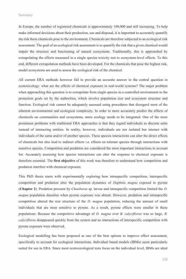
Summary
170
In Europe, the number of registered chemicals is approximately 100,000 and still increasing. To help
make informed decisions about their production, use and disposal, it is important to accurately quantify
the risk these chemicals pose to the environment. Chemicals are therefore subjected to an ecological risk
assessment. The goal of an ecological risk assessment is to quantify the risk that a given chemical would
impair the structure and functioning of natural ecosystems. Traditionally, this is approached by
extrapolating the effects measured in a single species toxicity test to ecosystem-level effects. To this
end, different extrapolation methods have been developed. For the chemicals that pose the highest risk,
model ecosystems are used to assess the ecological risk of the chemical.
All current ERA methods however fail to provide an accurate answer to the central question in
ecotoxicology: what are the effects of chemical exposure in real-world systems? The major problem
when approaching this question is to extrapolate from single species in a controlled environment to the
protection goals set by the authorities, which involve population size and ecosystem structure and
function. Ecological risk cannot be adequately assessed using procedures that disregard most of the
inherent environmental and ecological complexity. In order to more accurately predict the effects of
chemicals on communities and ecosystems, more ecology needs to be integrated. One of the most
prominent problems with traditional ERA approaches is that they regard individuals as discrete units
instead of interacting entities. In reality, however, individuals are not isolated but interact with
individuals of the same and/or of another species. These species interactions can alter the direct effects
of chemicals but also lead to indirect effects i.e. effects on tolerant species through interactions with
sensitive species. Competition and predation are considered the most important interactions to account
for. Accurately assessing how species interactions can alter the response to chemical exposure is
therefore essential. The first objective of this work was therefore to understand how competition and
predation interfere with chemical exposure.
This PhD thesis starts with experimentally exploring how intraspecific competition, interspecific
competition and predation alter the population dynamics of Daphnia magna exposed to pyrene
(Chapter 2). Predation pressure by Chaoborus sp. larvae and intraspecific competition limited the D.
magna population densities when pyrene exposure was absent. However, predation and intraspecific
competition altered the size structure of the D. magna population, reducing the amount of small
individuals that are most sensitive to pyrene. As a result, pyrene effects were smaller in these
populations. Because the competitive advantage of D. magna over B. calyciflorus was so large, B.
calyciflorus disappeared quickly from the system and no interactions of interspecific competition with
pyrene exposure were observed.
Ecological modelling has been proposed as one of the best options to improve effect assessment,
specifically to account for ecological interactions. Individual based models (IBMs) seem particularly
suited for use in ERA. Since most ecotoxicological tests focus on the individual level, IBMs are ideal

Summary
171
tools to translate these test results to the population and community level. However, current IBM
applications have neglected possible interactions with other species, despite this being one of the main
criticisms on current ERA methods. A second objective of this thesis was to develop an IBM framework
capable of predicting chemical effects on interacting species.
In Chapter 3, an individual-based modelling (IBMs) implementation was developed that accounted for
interactions between species. IBMs are ideal tools to simulate effects of chemicals on populations but
need to be based on a sound theoretical basis. Dynamic energy budget theory based on the keep it simple,
stupid principle (DEBkiss) offers a good compromise between complexity and the amount of data
required to parameterize the model. IBMs based on the DEBkiss theory were developed and chemical
effects on survival were implemented. Two possible methods to calculate the effects of chemicals were
included: concentration-response curves (CR) and toxicokinetic toxicodynamic models (TKTD). In
order for models to be trustworthy, they need to be validated i.e. their predictions need to be compared
with observations. Therefore, in Chapter 4, DEBkiss IBMs were parameterized for D. magna and B.
calyciflorus and compared to the outcome of the experiments of Chapter 2. The population dynamics of
isolated B. calyciflorus were accurately predicted using the DEBkiss IBM. Population dynamics of
isolated D. magna populations were reasonably predicted but not the size structure of the population.
This was attributed to the absence of a reserve compartment in the models, leading to faster starvation
when food is limited. Both toxicity models predicted pyrene effects that occurred sooner than observed
but the TKTD model approached the observed effects best. The outcome of competition was accurately
predicted when both DEBkiss IBMs were coupled to a shared food source: D. magna quickly
outcompeted B. calyciflorus. Using the models to simulate competition when exposed to pyrene resulted
in an increase of B. calyciflorus when D. magna densities decreased. This was not observed in the
experiments but was attributed to the predicted effects of pyrene occurring earlier in the simulations
than in the experiments.
Ecological risk assessment does not aim to protect one or two species in the laboratory but to protect
realistic communities in the field. A third objective of this work was to develop an IBM-based
modelling approach to account for chemical effects on higher ecological levels in realistic conditions.
ChimERAfoodweb was developed as a novel approach (Chapter 5): a food web model based on DEBkiss
IBMs. To achieve this, a newly implemented predation interaction was added to the earlier
implementation of competition between DEBkiss IBMs. The food web included two grazers
(Brachionus and Daphnia) and their predator (Chaoborus) and two detritus feeders (Asellus and
Gammarus). In order to perform simulations for realistic conditions, ChimERAfoodweb was coupled with
ChimERAfate to form the integrated ChimERA model. ChimERAfate is a dynamic and spatially explicit
fate model that predicts environmental concentrations based on environmental variables
(hydrodynamics, temperature and trophic state).
Summary
172
The integrated ChimERA model was developed as a tool to perform more realistic ecological risk
assessments. To test its application, the ChimERA model was applied to a two-pond system in 15
hypothetical scenarios (Chapter 6), differing in water residence time, temperature, trophic state and the
applied chemical. These differences in environmental conditions greatly determined the effects of
chemical exposure and large differences were predicted between the different scenarios. The physico-
chemical properties of the chemical determined the spatiotemporal pattern of the exposure i.e. where
and when the concentrations were highest and how fast the chemical disappeared. Concentrations of
applied chemicals were highest in scenarios with a high water residence time. Direct effects on
Chaoborus, Daphnia and Gammarus were predicted, as expected from the sensitivities of these species.
These effects however differed greatly between environmental scenarios, with more pronounced effects
in scenarios with a high trophic state and temperature. Within one scenario, the effects of the chemicals
on food web dynamics were heterogeneously distributed in space and time, following the differences in
exposure. The most notable indirect effects were a shift in dominance from Daphnia and Gammarus to
Brachionus and Asellus, respectively. Also, the predator Chaoborus was affected indirectly through
effects on its prey species Daphnia. The effects of the mixture of three chemicals differed between
species, where the effects of pyrene dominated for Daphnia and the effects of carbendazim and
chlorpyrifos for Gammarus. These simulations demonstrate how much the outcome of chemical
exposure is determined by environmental conditions and how important it is to account for these
environmental conditions in ERA through the use of models such as the ChimERA model.
In Chapter 7, the main conclusions and proposals for future research directions are given. This work
has shown how essential it is to approach the risk assessment of chemicals from an ecological
perspective. Species are not isolated entities but interact and influence the outcome of chemical
exposure. The ChimERA model developed and applied here is an important proof of principle on how
these interactions can be accounted for. More than this, the model also accounted for spatiotemporal
differences in exposure and effects of chemicals. The ChimERA model, when further tested and if
necessary extended, can serve as a blueprint for future efforts to model how chemicals affect realistic
systems.

173
SAMENVATTING

Samenvatting
174
Meer dan 100,000 verschillende chemicaliën zijn reeds geregistreerd in Europa. Om geïnformeerde
keuzes te maken omtrent de productie, het gebruik en het verwerken van deze chemicaliën is het
belangrijk om hun risico voor het milieu accuraat in te schatten. Dit wordt gedaan aan de hand van
ecologische risico-evaluaties. Ecologische risico-evaluaties hebben als doel het risico van chemicaliën
voor de structuur en het functioneren van natuurlijke ecosystemen te kwantificeren. Dit wordt
traditioneel benaderd door de effecten gemeten met een toxische test op één soort te extrapoleren naar
het ecosysteem-niveau. Hiervoor werden verschillende extrapolatietechnieken ontwikkeld en voor de
chemicaliën die het grootste risico vormen worden testen met modelecosystemen uitgevoerd.
Alle huidige ecologische risicoschatting technieken slagen er echter niet in een accuraat antwoord te
geven op de centrale vraag in ecotoxicologie: wat zijn de effecten van chemicaliën in realistische
ecosystemen? Het grootste probleem is hoe de effecten die gemeten zijn voor, in het beste geval,
modelgemeenschappen in gecontroleerde omstandigheden te extrapoleren naar de
beschermingsdoelstellingen vastgelegd door overheidsinstanties. Het ecologische risico kan niet
accuraat berekend worden met technieken die voorbij gaan aan de inherente complexiteit van ecologie.
Om het risico van chemicaliën voor gemeenschappen en het milieu beter in te schatten moet meer
rekening gehouden worden met de ecologische realiteit. Eén van de grootste problemen met de huidige
technieken voor ecologische risicoschatting is dat organismen als discrete eenheden worden beschouwd.
In werkelijkheid interageren organismen met andere organismen van dezelfde en/of een andere soort.
Deze soorteninteracties kunnen zowel de directe effecten van chemicaliën op gevoelige soorten
beïnvloeden als de indirecte effecten, d.w.z. de effecten die ontstaan door interacties met tolerante
soorten. Competitie en predatie worden algemeen beschouwd als de meest belangrijke types van
soorteninteracties. Nauwkeurig inschatten hoe deze soorteninteracties de effecten van een chemische
stof beïnvloeden is daarom essentieel.
De eerste doelstelling van dit doctoraatswerk was dan ook om te begrijpen hoe competitie en predatie
de effecten van chemicaliën kunnen beïnvloeden.
Dit doctoraatsonderzoek begint met experimenteel na te gaan hoe intraspecifieke competitie,
interspecifieke competitie en predatie een populatie van Daphnia magna beïnvloeden wanneer die
blootgesteld wordt aan pyreen (Hoofdstuk 2). Lagere densiteiten van D. magna werden vastgesteld
wanneer de populatie blootgesteld werd aan predatie door Chaoborus sp. larven of intraspecifieke
competitie. Deze twee soorteninteracties leidden er ook toe dat grote individuen talrijker waren. Grote
individuen zijn resistenter tegen pyreen effecten en de effecten van pyreen op de D. magna densiteit
waren dan ook kleiner wanneer de populatie ook blootgesteld was aan predatie of intraspecifieke
competitie. Omdat D. magna een veel sterkere competitor was dan B. calyciflorus had interspecifieke
competitie, onafhankelijk van de blootstelling aan pyreen, weinig invloed op de D. magna densiteiten.

Samenvatting
175
Ecologische modellen worden gesuggereerd als één van de beste opties om het inschatten van de
ecologische effecten van chemicaliën te verbeteren. Individu-gebaseerde modellen (IBMs) in het
bijzonder zijn uitermate geschikt om de gemeten effecten in standaard ecotoxicologische testen te
extrapoleren naar populatie- en gemeenschapsniveau. De huidige toepassingen van IBMs houden echter
geen rekening met hoe soorteninteracties de effecten van chemicaliën kunnen beïnvloeden. De tweede
doelstelling van dit doctoraat was dan ook om een IBM te ontwikkelen waarmee de interacties tussen
soorten kunnen in rekening gebracht worden.
In hoofdstuk 3 werd een IBM model ontwikkeld om twee soorten in competitie met elkaar te
modelleren. IBMs moeten een goede theoretische basis hebben om algemeen toepasbaar te zijn. De
“Dynamic energy budget” theorie gebaseerd op het “keep it simple, stupid” principe (DEBkiss) werd
gekozen omwille van de goede balans tussen complexiteit en benodigde data om het model te
parameteriseren. Als nieuwe aanpak om chemische effecten te voorspellen werden deze DEBkiss IBMs
gekoppeld met twee verschillende toxiciteitsmodellen :concentratie-effect curves en toxicokinetische-
toxicodynamische (TKTD) modellen. Als modelvalidatie werden de DEBkiss IBMs simulaties
vergeleken in hoofdstuk 4 met de resultaten van de experimenten uit hoofdstuk 2. De
populatiedensiteiten van B. calyciflorus werden accuraat voorspeld aan de hand van een DEBkiss IBM.
De populatiedensiteit van D. magna werd redelijk accuraat voorspeld maar de voorspelde
populatiestructuur week af van de geobserveerde. De afwezigheid van een reserve compartiment in de
DEBkiss theorie was waarschijnlijk de oorzaak, waardoor de individuen sneller verhongerden wanneer
voedsellimitatie optrad in de simulaties in vergelijking met de experimenten. De effecten van pyreen
werden door beide toxiciteitsmodellen te snel voorspeld, maar deze afwijking was kleiner voor het
TKTD model. Net als in de experimenten nam de B. calyciflorus populatie snel af door competitie met
D. magna. Wanneer de twee soorten in competitie blootgesteld werden aan pyreen werd een toename
van B. calyciflorus voorspeld. Dit werd niet waargenomen in de experimenten en was het gevolg van de
te vroeg voorspelde effecten van pyreen op D. magna.
Het doel van ecologische risicoschattingen is niet het beschermen van enkele soorten in het labo maar
het beschermen van gemeenschappen in het veld. Een laatste doelstelling van dit doctoraat was dan ook
om een model op basis van IBMs te ontwikkelen waarmee de effecten van chemicaliën op
gemeenschapsniveau kunnen ingeschat worden in realistische omstandigheden. Als een nieuwe aanpak
werd in hoofdstuk 5 het ChimERAfoodweb model ontwikkeld op basis van de hier ontwikkelde DEBkiss
IBMs. Predatie werd geïmplementeerd voor DEBkiss IBMs en gekoppeld aan de eerder ontwikkelde
implementatie voor competitie. Het gemodelleerde voedselweb bestond uit twee grazers (Brachionus en
Daphnia), hun predator (Chaoborus) en twee detritivoren (Asellus en Gammarus). Dit
voedselwebmodel werd gekoppeld aan ChimERAfate, een omgevingsmodel om de concentratie aan
chemicaliën te voorspellen. Het geïntegreerde ChimERA model kan voor een opgegeven
Samenvatting
176
landschapsstructuur de effecten van een chemische stof op het voedselweb voorspellen doorheen de tijd
op basis van opgegeven omgevingsvariabelen (hydrodynamica, temperatuur en nutriëntenstatus).
Het geïntegreerde ChimERA model werd ontwikkeld om meer realistische ecologische
risicoschattingen uit te voeren. Om dit te testen werd het toegepast voor 15 hypothetische scenario’s op
een landschap van twee geconnecteerde vijvers (Hoofdstuk 6). De retentietijd van water, temperatuur,
nutriëntenstatus en toegevoegde chemische stof (carbendazim, chlorpyrifos en pyreen) werden
aangepast tussen deze 15 scenario’s. De verschillen in omgevingsvariabelen bepaalden in grote mate de
voorspelde effecten van blootstelling aan chemicaliën en grote verschillen werden dan ook vastgesteld
tussen de verschillende scenario’s. Chemische concentraties waren het hoogst in scenario’s met een
hoge retentietijd. De fysicochemische eigenschappen van een chemische stof bepaalden waar en
wanneer de concentraties het hoogst waren en hoe snel de stof terug verdween uit de omgeving. Directe
effecten van de blootstelling aan chemicaliën werden voorspeld voor de meest gevoelige soorten
(Chaoborus, Daphnia en Gammarus). Deze voorspelde effecten vertoonden grote verschillen tussen de
gekozen scenario’s en waren in het algemeen groter wanneer de nutriëntenstatus en de temperatuur hoog
waren. In een scenario waren de voorspelde effecten van de chemicaliën heel heterogeen verdeeld in
tijd en ruimte als gevolg van de grote spatiotemporele verschillen in blootstelling,. De meest
voorkomende indirecte effect was het veranderen in dominantie van Daphnia en Gammarus naar
respectievelijk Brachionus en Asellus. Indirecte effecten van blootstelling werden ook voorspeld op de
predator Chaoborus via effecten op de gevoelige prooisoort Daphnia. Bij blootstelling aan het mengsel
van alle drie de chemicaliën domineerden de effecten van pyreen voor Daphnia en de effecten van
carbendazim en chlorpyrifos voor Gammarus. Deze scenariosimulaties tonen aan hoe groot de invloed
van omgevingsvariabelen is op de effecten van blootstelling aan chemicaliën en hoe belangrijk het dus
is om technieken zoals het ChimERA model te ontwikkelen..
In hoofdstuk 7 wordt een overzicht van de belangrijkste conclusies per hoofdstuk gegeven en worden
mogelijke pistes voor verder onderzoek aangereikte. Dit doctoraatsonderzoek heeft aangetoond hoe
essentieel het is om ecologische risicoschattingen te benaderen vanuit een ecologische invalshoek.
Soorten zijn geen geïsoleerde eenheden maar interageren en bepalen wat de effecten zijn van
blootstelling aan een chemische stof. Het hier ontwikkelde ChimERA model is een belangrijk “proof of
principle” waarmee werd aangetoond hoe soorteninteracties kunnen in rekening gebracht worden. Meer
dan dat, dit model was in staat om spatiotemporele verschillen in blootstelling en effecten van
chemicaliën te voorspellen op gemeenschapsniveau. Het ChimERA model, wanneer het nog verder
getest en uitgebreid wordt, kan als blauwdruk dienen voor toekomstige modellen en leiden tot meer
realistische ecologische risicoschattingen.

177
DANKWOORD
Dankwoord
178
Mijn doctoraat is het eindresultaat van een bijna vijfjarige, intense reis. Gedurende die reis heb ik lief
en leed gedeeld met vele mede-reizigers die ik hier wil bedanken voor de vele mooie ervaringen.
Laat mij eerst beginnen bij de “reisleiders”, Colin en Frederik, want zonder hen was deze reis er niet
geweest. Colin, bedankt om mij als verloren gelopen bioloog de kans te geven om te beginnen aan het
labo. Ondanks het niet halen van mijn IWT-beurs heb je me toch de kans gegeven om te blijven werken
op interessante projecten. Je gezonde scepticisme voor het modelleren zorgde ook altijd voor de nodige
reality check. En nog eens extra bedankt om er op het einde nog een serieuze duw aan te geven bij het
schrijven, mijn doctoraat is er zeker nog een stuk beter door geworden. Frederik, ik weet niet goed waar
te beginnen. Dankzij jou ben ik in dit doctoraat gerold en ik heb niet meer omgekeken. Al van in het
begin gaf je me zo veel vertrouwen en vrijheid. We hebben samen veel rondgereisd (Noorwegen, Como,
Berlijn) en ik kan je niet genoeg bedanken voor alle kansen die je me gegeven hebt. Je stond, en staat,
altijd klaar met goede raad en oplossingen wanneer het wat minder ging. Je had er altijd het volste
vertrouwen in wanneer ik aan iets nieuws begon en ik wist dat ik op je kon terugvallen als ik vast zat.
En je hield ook altijd de menselijke kant in de gaten. Bedankt om zo geduldig te zijn, zo begrijpzaam,
mij zo veel bij te leren en mij te steunen door dik en dun.
De vaste reisgenoten waren natuurlijk de collega’s van de Plateau. En de reis zou niet half zo leuk
geweest zijn zonder jullie! De gezellige koffiepauzes (die verassend vaak uitliepen), een “Brugske” doen
(of waren het burgers?) over de middag, het pintje na de uren dat we ons af en toe toch eens beklaagd
hebben “the day after”, de legendarische SETAC-congressen, het zijn allemaal reiservaringen die ik niet
snel ga vergeten. Een aantal personen wil ik hierbij nog eens extra bedanken. Als eerste, mijn roomie
Tina. De toffe babbels, de lachmomenten, de gezamenlijk powerpointsessies, ja, ik zal onze “oase van
rust“ echt missen. David, Lisbeth en Charlotte, we leggen al dezelfde reisweg af sinds we samen biologie
zijn begonnen en het zou absoluut niet hetzelfde geweest zijn zonder jullie. David, mijn vaste bunk
buddy, merci om zo vaak mijn klankbord te zijn en altijd klaar te staan, ik weet gewoon dat wij elkaar
zullen blijven horen. Maarten, ik heb het gevoel dat ik je eigenlijk al gans mijn leven ken. Ik zal je
ongezouten uitspraken zeker missen! En laat me de andere Stickers niet vergeten: Jenny, de gin-tonics
met jou erbij waren altijd de beste. Jan, vogels zullen nooit meer dezelfde zijn na jou. Emmanuel,
ondertussen ben je toch ook officieel een Sticker. Bedankt voor de vele onvergetelijke uren op het labo
en erbuiten! Cecilia, you are my favourite Portuguese person! Thanks for all the great talks and laughs.
Tara, altijd lief en zorgzaam. Wanneer is de volgende spelletjesavond met pannenkoeken (ja, ik ben
mezelf weer aan het uitnodigen)? Sacha, je dagelijkse bezoekje was een welgekomen verstrooiing
tijdens het schrijven. Marianne, Sigrid en Veerle: bedankt voor alle steun, zowel administratief als in de
vorm van een snoep en een babbel. Nancy, ik heb niet veel in het labo gestaan in Gent, maar ik kon toch
altijd terecht bij je voor praktische vragen. En ik vergeet ongetwijfeld nog veel andere mensen, sorry
daarvoor! Ik weet niet waar de reis nu naartoe gaat, maar als mijn toekomstige reisgenoten half zo leuk
zijn als jullie, zal ik mezelf heel gelukkig prijzen.
Dankwoord
179
Tijdens mijn doctoraatsreis werd er ook veel samengewerkt met buitenlandse collega’s. Aan de mensen
van Wageningen, bedankt voor alles, de tijd in Nederland is echt voorbij gevlogen. Andreas en Hans,
dit doctoraat zou er niet geweest zijn zonder jullie hulp. De vele mails, skype sessies en blitzbezoeken
aan Wageningen, jullie stonden altijd klaar voor me. Ik ga onze gezamenlijke modelleersessies missen.
Zoals afgesproken gaan we zeker nog eens een pintje drinken. Paul, bedankt voor de kans om bij jullie
op het labo te werken, ik voelde me er echt thuis. De mensen van het labo in Wageningen wil ik zeker
ook bedanken: Ana and Andreu, thanks for making the long days in the lab so enjoyable. Dimitri, ik wil
je hier nog eens extra bedanken om me op weg te zetten in Wageningen en voor de babbels met onze
hoofden boven de microcosmossen. John, Frits, Wendy, bedankt voor alle technische steun.
Ook bedankt aan de mensen van Nijmegen voor de vlotte samenwerking. En Lisette, onze rondreis in
de Lofoten zal me zeker altijd bijblijven. Veel succes met je verdediging! To the colleagues from Como:
thanks for the great co-operation. Thanks to you, fate models seem less scary now! Melissa, thanks for
being my co-PhD student in the ChimERA project, it was great to have somebody to share laughs with.
Tijdens mijn doctoraatsreis kreeg ik ook vaak het gezelschap van enkele oude bekenden. Karen, er is
veel gebeurd tussen ons, maar je hebt me zeker door een groot deel van dit doctoraat geholpen. Matthias
en Sarah, dankzij jullie was Brugge één van de terugkerende reisbestemmingen. Zoals je weet, Matthias,
is het leven van een doctoraatstudent toch hard he! Bedankt voor mij te pushen wanneer ik weer eens te
veel slabakte en om gewoon een goeie maat te zijn. Wanneer brouwen we nog eens? Nuyttens en Tjorre,
beste vrienden, we kennen elkaar al zo lang en ik vind het echt de max dat we blijven contact houden.
Dit doctoraat is er ook gekomen dankzij jullie steun tijdens brunches of spelletjesavonden. Samuel,
roomie, merci om zo relaxt te zijn. De vele boardgames, hots-kes en frisbee sessies hebben zeker
geholpen om de stress te beperken. Thokie, ik ben echt blij dat we zo goed blijven overeen komen.
Wanneer is de volgende roadtrip? Robin en Kevin, merci om er altijd te zijn, al zo lang.
Ten slotte, er is niets zo leuk als te weten dat je na een lange reis altijd welkom bent bij het thuisfront.
Mama en papa, merci om me altijd mijn ding te laten doen maar er toch te staan wanneer het nodig is.
Ik zou nooit zo ver geraakt zijn zonder jullie, mijn veilige thuishaven. Thomas, Charlotte en Jozefien
bedankt om mij te steunen door dik en dun, het heeft echt deugd gedaan om te weten dat jullie er waren.
De reis gaat nu verder, ik weet niet waarheen. Maar ik kijk alvast met een brede glimlach terug op de
reeds afgelegde weg.


181
CURRICULUM VITAE

Curriculum vitae
182
PERSONALIA
Surname: Viaene First name: Karel Address: Koningin Astridlaan 145
B-9000 Gent E-mail: [email protected]: 0496/49 70 24Date of birth: 6 juli 1987 Place of birth: Izegem Nationality: Belgium
PROFESSIONAL EMPLOYMENT
2011-Present PhD Student at the Laboratory of Environmental Toxicology and Aquatic Ecology, Ghent University, Belgium
EDUCATION
2010 – 2011 Master in de Milieusanering en het Milieubeheer Ghent University
Master thesis: Long-term changes in the Barents Sea: Modelling the effects of fisheries, organic pollutants, climate and ecological interactions on Gadus morhua. Promotor: Prof. Dr. Colin Janssen Co-promotor: Dr. Ir. Frederik De Laender
With distinction
2008 – 2010 Master in Biology Ghent University Majors: Ecology – Evolution
Master Thesis: Phylogeny and ecophysiology of Cylindrotheca closterium and the consequences for ecosystem functioning. Promotor: Prof. Dr. Wim Vyverman Co-promotor: Prof. Dr. Koen Sabbe
With great distinction
2005 –2008 Bachelor in Biology Ghent University
Bachelor thesis: Speelt de verwantschap tussen soorten een rol in de relatie tussen diversiteit en productiviteit? Promotor: Prof. Dr. Koen Sabbe Co-promotor: Prof. Dr. Wim Vyverman
GRANTS
FWO Travelling Grant for a Long Stay Abroad at Aquatic Ecology and Water Quality Management Group, Wageningen University and Research Centre, Wageningen, The Netherlands. 1 August 2013 - 30 September 2013
FWO Travelling Grant for a Long Stay Abroad at Aquatic Ecology and Water Quality Management Group, Wageningen University and Research Centre, Wageningen, The Netherlands. 18 May 2014 – 18 July 2014

Curriculum vitae
183
PUBLICATIONS
Viaene KPJ, De Laender F, Van den Brink PJ, Janssen CR. Using additive modelling to quantify the effect of chemicals on phytoplankton diversity and biomass. Science of the Total Environment. 2013; 449:71–80.
Viaene KPJ, Janssen CR, de Hoop L, Hendriks AJ, De Laender F. Evaluating the contribution of ingested oil droplets to the bioaccumulation of oil components--a modeling approach. Science of the Total Environment. 2014; 499:99–106.
De Hoop L, Huijbregts M a J, Schipper AM, Veltman K, De Laender F, Viaene KPJ, et al. Modelling bioaccumulation of oil constituents in aquatic species. Mar Pollut Bull. 2013;76(1-2):178–86.
Viaene KPJ, De Laender F, Rico A, Van den Brink PJ, Di Guardo A, Morselli M, et al. Species interactions and chemical stress: Combined effects of intraspecific and interspecific interactions and pyrene on Daphnia magna population dynamics. Environtal Toxicoly and Chemistry. 2015; 34(8):1751–9.
PLATFORM PRESENTATIONS
Viaene K.P.J., Janssen C.R., De Hoop L., Hendriks A.J. and De Laender F. Oil spills: never mind the droplets. Oral pitching presentation at the 13th VLIZ Young Marine Scientists’ Day, Bruges, 15 February 2013
Viaene K.P.J., Janssen C.R., De Hoop L., Hendriks A.J. and De Laender F. Models that ignore oil droplet uptake are sufficiently accurate to predict the bioaccumulation of oil-associated PAHs. Oral presentation at the 18th National Symposium on Applied Biological Sciences, Ghent, 8 February 2013
POSTER PRESENTATIONS
Viaene K.P.J., De Laender F., Van den Brink P.J., Janssen C.R. Inferring the effects of chemicals on biodiversity: a case study with the herbicide linuron. Poster presentation at the 6th SETAC World Congress, Berlin, 21-24 May 2012.
Viaene K.P.J., Janssen C.R., De Hoop L., Hendriks A.J., De Laender F. Models that ignore oil droplet uptake are sufficiently accurate to predict the bioaccumulation of oil-associated PAHs. Poster presentation at the 23th Annual Meeting SETAC Europe, Glasgow, 13-16 May 2013.
De Laender F., Viaene K.P.J., Di Guardo A., Morselli M., Baveco H., Van den Brink P. ChimERA: Coupling exposure and effects into a predictive integrated framework for risk assessment. Poster presentation at the 23th Annual Meeting SETAC Europe, Glasgow, 13-16 May 2013.
Viaene K.P.J., Rico A., Janssen C.R., van den Brink P.J., De Laender F. Ecological interactions alter the response of Daphnia magna populations to chemical stress. Poster presentation at the 24th Annual Meeting SETAC Europe, Basel, 11-15 May 2014.

Curriculum vitae
184
Viaene K.P.J., Focks A., Baveco H., van den Brink P.J., De Laender F., Janssen C.R. Coupled individual based models as a new tool to predict ecological effects in multi-species systems. Poster presentation at the 24th Annual Meeting SETAC Europe, Basel, 11-15 May 2014.
Viaene K.P.J., De Laender F., Di Guardo A., Morselli M., Janssen C.R. The ecological consequences of various chemical emission patterns in food webs. Poster presentation at the 24th Annual Meeting SETAC Europe, Basel, 11-15 May 2014.
Viaene K.P.J., Focks A., Baveco H., van den Brink P.J., Janssen C.R., De Laender F. Using the DEBkiss IBM framework to predict chemical effects on two interacting zooplankton species. Poster presentation at the 25th Annual Meeting SETAC Europe, Barcelona, 3-7 May 2015.
Viaene K.P.J., De Laender F., Janssen C.R. Food web models as a tool for ecological scenario analysis. Poster presentation at the 25th Annual Meeting SETAC Europe, Barcelona, 3-7 May 2015.
ATTENDED CONFERENCES AND WORKSHOPS
Society of Environmental Toxicology and Chemistry (SETAC), 6th World Congress, 20-24 May, Berlin, Germany
SETAC Europe, 23th Annual Meeting, Glasgow, UK.
SETAC Europe, 24th Annual Meeting, Basel, Switzerland.
SETAC Europe, 25th Annual Meeting, Barcelona, Spain.
National Symposium on Applied Biological Sciences, 18th Edition, 8 February 2013, Ghent, Belgium
VLIZ Young Marine Scientists’ Day, 13th Edition, 15 February 2013, Bruges, Belgium
MEMBERSHIP OF PROFESSIONAL ORGANIZATIONS
Member of the Society of Environmental Toxicology and Chemistry (SETAC)