the variational method - kfupm

Prof. Dr. I. Nasser Atomic and Molecular Physics Phys 551 (T-112) February 18, 2012 variational-methI_t112.doc

1

The Variational Method Introduction:

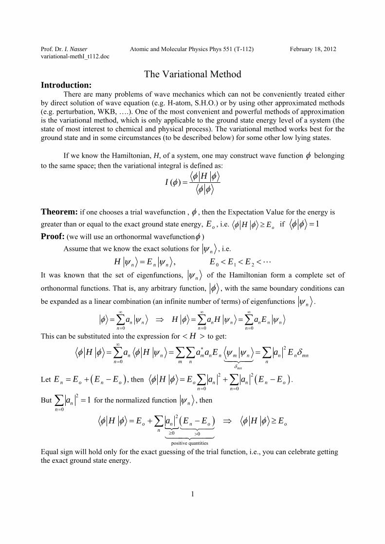
There are many problems of wave mechanics which can not be conveniently treated either by direct solution of wave equation (e.g. H-atom, S.H.O.) or by using other approximated methods (e.g. perturbation, WKB, ….). One of the most convenient and powerful methods of approximation is the variational method, which is only applicable to the ground state energy level of a system (the state of most interest to chemical and physical process). The variational method works best for the ground state and in some circumstances (to be described below) for some other low lying states.

If we know the Hamiltonian, H, of a system, one may construct wave function φ belonging to the same space; then the variational integral is defined as:

( )H

Iφ φ

φφ φ

=

Theorem: if one chooses a trial wavefunction , φ , then the Expectation Value for the energy is greater than or equal to the exact ground state energy, oE , i.e. oH Eφ φ ≥ if 1φ φ =

Proof: (we will use an orthonormal wavefunctionφ ) Assume that we know the exact solutions for nψ , i.e.

0 1 2, n n nH E E E Eψ ψ= < < <

It was known that the set of eigenfunctions, nψ of the Hamiltonian form a complete set of

orthonormal functions. That is, any arbitrary function, φ , with the same boundary conditions can

be expanded as a linear combination (an infinite number of terms) of eigenfunctions nψ .

0 0 0n n n n n n n

n n na H a H a Eφ ψ φ ψ ψ

∞ ∞ ∞

= = =

= ⇒ = =∑ ∑ ∑

This can be substituted into the expression for H< > to get: 2*

0

∞

=

= = =∑ ∑∑ ∑mn

n n m n n m n n n mnn m n n

H a H a a E a Eδ

φ φ φ ψ ψ ψ δ

Let ( )n o n oE E E E= + − , then ( )2 2

0 0= =

= + −∑ ∑o n n n on n

H E a a E Eφ φ .

But 2

01n

na

=

=∑ for the normalized function nψ , then

( )2

0 0

positive quantities

≥ >

= + − ⇒ ≥∑o n n o on

H E a E E H Eφ φ φ φ

Equal sign will hold only for the exact guessing of the trial function, i.e., you can celebrate getting the exact ground state energy.


2

Mathematically, the value 0E is known as the lower limit to the sequence of the value ( )I φ , which obtained by assuming reasonable values for φ . Usually the variational integral is depend upon a

parameter or a number of parameters, iλ , which could be determined by the condition 0i

dId λ

= .

The key in this approximation is a good guess of a trial wave function. You can make a good

guess of a trial wave function by considering:

1- Is the parity conserved? Is the wave function even or odd? 2- How does the wave function approach zero? Model the asymptotes correctly. 3- Pick something you can integrate. Numerical integration is appropriate if analytic integration

is not. The integral must converge in any instance.

Example: Use a trial function of the form 1 ( ) ars r Neϕ −= to calculate the ground state energy of

the hydrogen atom. [Note that: 2 11ˆ2 rH

r= − ∇ − , and 2 2

2

1r r

r r r∂ ∂

∇ =∂ ∂

].

Solution: First calculate the normalization constant N (use sin2d r d d drτ θ θ ϕ= ):

2

22 2 2 2

1 1 10 0 0

21 24

| ( ) sin∞

−< > = =∫ ∫ ∫ ∫ars s s

a

r d N r e dr d dπ π

π

ϕ ϕ ϕ τ θ θ ϕ

Using the standard integral: 2

30

2brr e drb

∞− =∫ , we can have

3/ 22

3

14 | | 14

aN Na

ππ

= ⇒ =

Second calculate 1 1ˆ| |= < >s sI Hϕ ϕ as follows:

3/ 21 12 2 1

1 2 2

22

1 12

1 1 1ˆ ( )2 2

1 1 (2 )2

−⎡ ∂ ⎤∂ ∂⎡ ⎤= − − = − − −⎢ ⎥ ⎢ ⎥∂ ∂ ∂⎣ ⎦⎣ ⎦⎡ ⎤−⎡ ⎤= − − = −⎢ ⎥⎢ ⎥⎣ ⎦ ⎣ ⎦

s s ar ss

s s

aH r r aer r r r r r r

a a ar r ar r r

ϕ ϕ ϕϕπ

ϕ ϕ

Then 2

* 2 3 2 21 1 1 1

0 0

2 23

2 3

1ˆ ˆ( ) 4 42

1! 2!4 ( 1)(2 ) 2 (2 ) 2

∞ ∞−⎡ ⎤−

= = = −⎢ ⎥⎣ ⎦

⎡ ⎤= − − = −⎢ ⎥

⎣ ⎦

∫ ∫ ars s s s

a aI a H H r dr a e r drr

a aa a aa a

ϕ ϕ π ϕ ϕ

Setting ( ) 0= ⇒dI a

da

2

1 0 12

⎡ ⎤∂ ∂= − = − = ⇒ =⎢ ⎥∂ ∂ ⎣ ⎦

I a a a aa a


3

And substituting this result back into ( )W a gives 2

1 min1 11 a.u.

2 2 2= = − = − = −

aE I a

This happens to be the exact ground state energy of a hydrogen atom. H.W1. Plot W versus a. to check the optimum value at a=1. H.W2. Calculate T and V and find the relation between them.

H.W3. Calculate T and V and find the relation between them.

H.W4. Use a trial function of the form 2

1 ( ) −= a rs r Neϕ to

calculate the ground state energy of the hydrogen atom.

Variational Method Treatment of Helium Recall that we proved earlier that, if one has an approximate “trial” wavefunction, φ , then

the expectation value for the energy must be either higher than or equal to the true ground state energy. It cannot be lower!!

0

*

*trial

H dHE E E

d

φ φ τφ φφ φ φ φ τ

< >= = = ≥∫∫

This provides us with a very simple “recipe” for improving the energy. The lower the better!! When we calculated the He atom energy using the “Independent Particle Method”, we obtained an energy (-4.0 a.u.) which was lower than experiment (-2.9037 au). Isn’t this a violation of the Variational Theorem?? No, because we did not use the complete Hamiltonian in our calculation. Example: Calculate the ground state energy for the Helium atom using the following trial function:

1 1 2 1 1 1 2( , ) ( ) ( )s s sr r r rψ ψ ψ= where

3

1 ( ) , , 1, 2ia rs i

ar N e N iψπ

−= = =

a is a variational parameter and 2

1 ( ) 1s i ir dψ =∫ r Answer: Start with the Hamiltonian:

)A.1 ( 2 21 2

1 2 12

1 1 2 2 1ˆ2 2

Hr r r

= − ∇ − ∇ − − +

And put it in a simple form:

)A.2 ( 2 21 2

1 2 1 2 12

1 1 ( 2) ( 2) 1ˆ2 2

a a a aHr r r r r

− −= − ∇ − − ∇ − + + +

Use the Hydrogen atom Hamiltonian in a.u.:

-0.6

-0.3

0

0.3

0.6

-0.6 0 0.6 1.2 1.8

a (Hartree)

W (H

artre

e)


4

)A.3 ( 2

21 ( ) ( )2 2i i i

i

a ar rr

ψ ψ⎛ ⎞− ∇ − = −⎜ ⎟⎝ ⎠

One finds: 2 2

* *1 1 1 2 1 1 1 2 1 2

1 2 12

( 2) ( 2) 1( ) ( ) ( ) ( ) ( )2 2

⎡ ⎤− −= − − + + +⎢ ⎥

⎣ ⎦∫ ∫ s s s s

a a a aI a r r r r d dr r r

ψ ψ ψ ψ τ τ

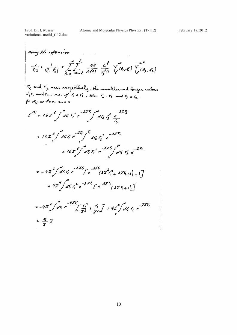
Taking into account the following integrations:

2 2

4− ±

=+∫

iar ie dr a q

πq r

r ;

( )1 22 2 22 2

1 2 2 1 1 1 1 2 21 2

1 1

4( ) ( )2

− − −

= =

= = =∫ ∫ ∫ ∫ ∫a r a r ar

s se e er d d r d d d

r r r aπψ τ τ ψ τ τ τ ;

and 2 2

1 1 1 2 1 22 1

1 5( ) ( ) ( )8

= =−∫ ∫ s s

aJ a r r d dψ ψ τ τr r

one finds: 3 2

2 2 22 ( 2) 5 27 ( ) ( ) 2 ( 2)8 8

−−= − + + = − + − + = −∫

ara a e aI a a d J a a a a a ar

τπ

To find the optimum value for a , we use the relation ( ) 0W aa

∂=

∂ to have

27 516 16

a Z= ≡ − and the

lowest energy is: 2 2

21 min

27 27 27 27 27 2.8477 a.u. 77.45 eV8 16 8 16 16

⎛ ⎞ ⎛ ⎞⎛ ⎞ ⎛ ⎞= = − = − = − = − = −⎜ ⎟ ⎜ ⎟⎜ ⎟ ⎜ ⎟⎝ ⎠ ⎝ ⎠⎝ ⎠ ⎝ ⎠

E I a a

The lower value for the “effective” atomic number (27

1.6916

' == =a Z vs. Z=2) reflects

“screening” due to the mutual repulsion of the electrons. 2.8477 a.u.=−trialE (1.9% higher than experiment) exp 2.9037 a.u.=−tE

The following table shows the theoretical and experimental values of ionization energy of the ground state energy for He-like atoms.

As we can see, the error decreases with increasing Z. One can improve (i.e. lower the energy) by employing improved wavefunctions with additional variational parameters.

error% Exp (eV)

Theo (eV)

Atom Z

5.31 24.5 23.2 He 2 1.98 75.6 74.1 +Li 3 0.91 153.6 152.2 ++Be 4 0.76 393 390 4+C 60.14 738 737 6+O 8


5

A Two Parameters Wavefunction

Let the two electrons have different values of Zeff: 1 2 1 2' '' '' 'Z r Z r Z r Z rA e e e eφ − − − −⎡ ⎤= +⎣ ⎦

(we must keep treatment of the radial part of the two electrons symmetrical, since the spin part is antisymmetrical) If one computes Etrial as a function of Z’ and Z’’ and then finds the values of the two parameters that minimize the energy, one finds:

Z’ = 1.19, Z’’ = 2.18, Etrial = -2.876 au (1.0% higher than experiment) The very different values of Z’ and Z’’ reflects correlation between the positions of the two electrons; i.e. if one electron is close to the nucleus, the other prefers to be far away. Another Wavefunction Incorporating Electron Correlation

( )1 2'( )121Z r rA e b rφ − +⎡ ⎤= + ⋅⎣ ⎦

When Etrial is evaluated as a function of Z’ and b, and the values of the two parameters are varied to minimize the energy, the results are:

Z’ = 1.19, b = 0.364 and Etrial = -2.892 au (0.4% higher than experiment). The second term, ( )121+ ⋅b r , accounts for electron correlation. It increases the probability (higher

φ2) of finding the two electrons further apart (higher 12r ).

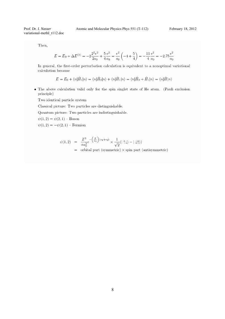
Notes: 1- The computed energy is always higher than experiment. 2- One can compute an “approximate” energy to whatever degree of accuracy desired. 3- The choice of a = Z reduces to the first-order perturbation theory in the previous section, which is

therefore equivalent to a ”non-optimum" variation calculation. 4- The physical meaning of a is that it represents the “effective charge" of the nucleus. The optimum a is

less than Z (the true nuclear charge) because the electron experiences the screening effect of the other electron.


6


7


8


9


10


11


12


13

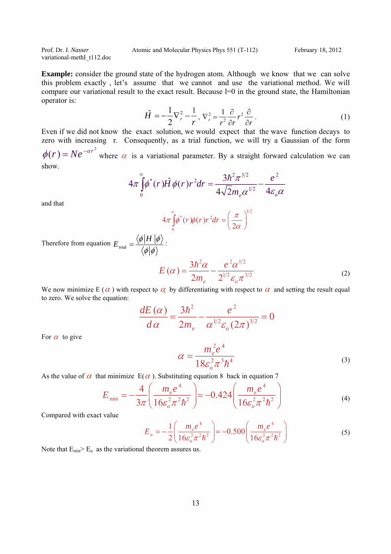
Example: consider the ground state of the hydrogen atom. Although we know that we can solve this problem exactly , let’s assume that we cannot and use the variational method. We will compare our variational result to the exact result. Because l=0 in the ground state, the Hamiltonian operator is:

2 11ˆ2 rH

r= − ∇ − , 2 2

2

1r r

r r r∂ ∂

∇ =∂ ∂

. (1)

Even if we did not know the exact solution, we would expect that the wave function decays to zero with increasing r. Consequently, as a trial function, we will try a Gaussian of the form

2

( ) rr Ne αφ −= where α is a variational parameter. By a straight forward calculation we can show.

2 3 2 2* 2

1 20

3ˆ4 ( ) ( )44 2 oe

er H r r drmππ φ φ

ε αα

∞

= −∫

and that 3 2

* 2

0

4 ( ) ( )2

r r r dr ππ φ φα

∞ ⎛ ⎞= ⎜ ⎟⎝ ⎠∫

Therefore from equation trial

HE

φ φφ φ

= :

2 2 1 2

1 2 3 2

3( )2 2e o

eEmα αα

ε π= − (2)

We now minimize E (α ) with respect to α by differentiating with respect to α and setting the result equal to zero. We solve the equation:

2 2

1 2 3 2

( ) 3 02 (2 )e o

dE ed mαα α ε π

= − =

For α to give 2 4

2 3 418e

o

m eαε π

= (3)

As the value of α that minimize E(α ). Substituting equation 8 back in equation 7

4 4

min 2 2 2 2 2 2

4 0.4243 16 16

e e

o o

m e m eEπ ε π ε π⎛ ⎞ ⎛ ⎞

= − = −⎜ ⎟ ⎜ ⎟⎝ ⎠ ⎝ ⎠

(4)

Compared with exact value 4 4

2 2 2 2 2 2

1 0.5002 16 16

e eo

o o

m e m eEε π ε π

⎛ ⎞ ⎛ ⎞= − = −⎜ ⎟ ⎜ ⎟

⎝ ⎠ ⎝ ⎠ (5)

Note that Emin> Eo as the variational theorem assures us.


14

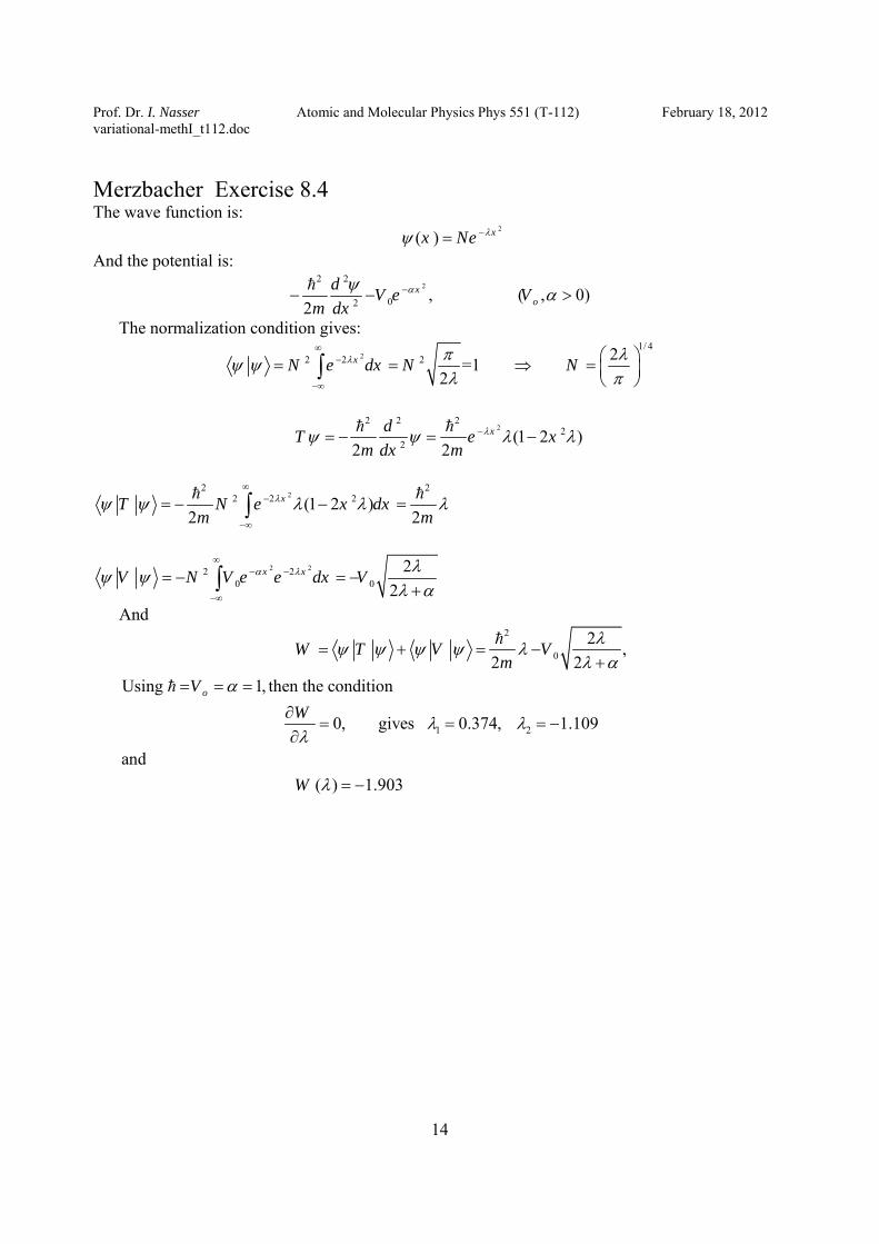
Merzbacher Exercise 8.4 The wave function is:

2

( ) xx Ne λψ −= And the potential is:

22 2

02 , ( , 0)2

xo

d V e Vm dx

αψ α−− − >

The normalization condition gives: 2

1/ 42 2 2 2=1

2xN e dx N Nλ π λψ ψ

λ π

∞−

−∞

⎛ ⎞= = ⇒ = ⎜ ⎟⎝ ⎠∫

2

2 2 22

2 (1 2 )2 2

xdT e xm dx m

λψ ψ λ λ−= − = −

2

2 22 2 2(1 2 )

2 2xT N e x dx

m mλψ ψ λ λ λ

∞−

−∞

= − − =∫

2 22 2

0 02

2x xV N V e e dx Vα λ λψ ψ

λ α

∞− −

−∞

= − = −+∫

And 2

0

1 2

2 ,2 2

Using 1, then the condition

0, gives 0.374, 1.109

and

o

W T V Vm

VW

λψ ψ ψ ψ λλ α

α

λ λλ

= + = −+

= = =

∂= = = −

∂

( ) 1.903W λ = −


15

Merzbacher Exercise 8.5 The wave function is:

(1 ), ( )

0,

xC x a

x ax a

ψ⎧

− ≤⎪= ⎨⎪ ≥⎩

And the potential is: 2 2

22

12 2

d kxm dx

ψ− +

The normalization condition gives:

2 2

0 02 2 2

/3 /3

2

(1 )

(1 ) (1 )

2 31 C=3 2a

a

a

a a

a a

xC dx

a

x xC dx dxa a

aC

ψ ψ−

− −

= −

⎧ ⎫⎪ ⎪⎪ ⎪= + + −⎨ ⎬⎪ ⎪⎪ ⎪⎩ ⎭

⎧ ⎫= = ⇒⎨ ⎬⎩ ⎭

∫

∫ ∫

Note that: we will use the integral: 22

* *2

0

d d ddx dxdx dx dxψ ψ ψψ ψ

∞∞ ∞

−∞−∞ −∞

=

⎛ ⎞= − ⎜ ⎟⎝ ⎠∫ ∫

The expectation of T and V gives: 2 2

22

22 2

2

2/

(1 ) (1 )2

3 3(1 )2 2a 2 a

a

a

a

a

a

x xdT C dxm a dx a

xd dxm dx a m

ψ ψ−

−

−

= − − −

⎛ ⎞= − − =⎜ ⎟

⎝ ⎠

∫

∫

3 3

2 2

0 02 2 2 2 2

/30 /30

3 2

1 (1 ) (1 ) , 2

1 (1 ) (1 )2

1 3 22 2a 30 20

a

a

a a

a a

x xV k x dx k m

a a

x xkC x dx x dxa a

a ak k

ψ ψ ω−

− −

= − − =

⎧ ⎫⎪ ⎪⎪ ⎪= + + −⎨ ⎬⎪ ⎪⎪ ⎪⎩ ⎭

= =

∫

∫ ∫

And


16

2 2

2

1/ 424

2 2

3 ,2 a 20

The condition

30 30 0, gives a = m k

and

aW T V km

W aa m

ψ ψ ψ ψ

ω

= + = +

∂ ⎛ ⎞= ⇒ = ⎜ ⎟∂ ⎝ ⎠

0.5447 0.5 , as expected W ω ω= >

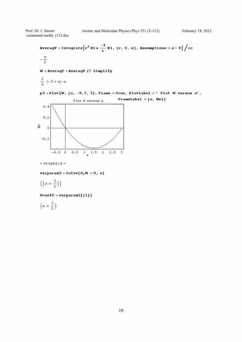
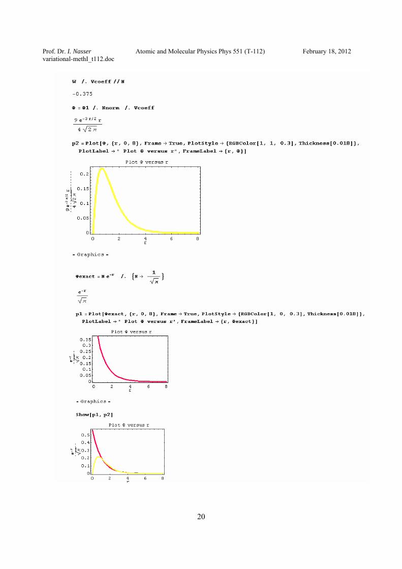
1- Apply the variational method to the determination of the ground state energy of the hydrogen atom, using ( , ) brr b Areψ −= as a trial function. Here, A is the normalization constant and b is the variational parameter.

a. calculate .N b. calculate .T

c. calculate .V d. calculate ( ).W b e. calculate .b f. calculate min .E

Discuss your final result, for example: compared with the exact, the behavior of the wave

function. [Hint: 22

1 1ˆ ,2

T rr r r

∂ ∂⎡ ⎤= − ⎢ ⎥∂ ∂⎣ ⎦ 1( )V r

r= − ]


17

Answer:


18


19


20


21

Comment: -0.375 > -0.5 which satisfy the variational approximation claim. The difference is mainly due to the behavior of the wave function at the origin.


22

the variational method - kfupm

Documents