The Value of Medicaid: Interpreting Results from the OregonHealth Insurance Experiment

Amy Finkelstein, Nathaniel Hendren, and Erzo F.P. Luttmer∗

April 2018

Abstract

We develop a set of frameworks for welfare analysis of Medicaid and apply them to the Ore-gon Health Insurance Experiment, a Medicaid expansion for low-income, uninsured adults thatoccurred via random assignment. Across different approaches, we estimate recipient willingnessto pay for Medicaid between $0.5 and $1.2 per dollar of the resource cost of providing Medicaid;estimates of the expected transfer Medicaid provides to recipients are relatively stable acrossapproaches, but estimates of its additional value from risk protection are more variable. Wealso estimate that the resource cost of providing Medicaid to an additional recipient is only 40%of Medicaid’s total cost; 60% of Medicaid spending is a transfer to providers of uncompensatedcare for the low-income uninsured.

1 Introduction

Medicaid is the largest means-tested program in the United States. In 2015, public expenditureson Medicaid were over $550 billion, compared to about $70 billion for food stamps (SNAP), $70billion for the Earned Income Tax Credit (EITC), $60 billion for Supplemental Security Income(SSI), and $30 billion for cash welfare (TANF).1 How much would recipients be willing to payfor Medicaid and how does this compare to Medicaid’s costs? And how much of Medicaid’s costsreflect a monetary transfer to non-recipients who bear some of the costs of covering the low-incomeuninsured?

There is a voluminous academic literature studying the reduced-form impacts of Medicaid ona variety of potentially welfare-relevant outcomes – including health care use, health, and risk

∗MIT, Harvard, and Dartmouth. We are grateful to Lizi Chen for outstanding research assistance and to IsaiahAndrews, David Cutler, Liran Einav, Matthew Gentzkow, Jonathan Gruber, Conrad Miller, Jesse Shapiro, MatthewNotowidigdo, Ivan Werning, three anonymous referees, Michael Greenstone (the editor), and seminar participants atBrown, Chicago Booth, Cornell, Harvard Medical School, Michigan State, Pompeu Fabra, Simon Fraser University,Stanford, UCLA, UCSD, the University of Houston, and the University of Minnesota for helpful comments. Wegratefully acknowledge financial support from the National Institute of Aging under grants RC2AGO36631 andR01AG0345151 (Finkelstein) and the NBER Health and Aging Fellowship, under the National Institute of AgingGrant Number T32-AG000186 (Hendren).

1See Department of Health and Human Services (2015, 2016)[49, 50], Department of Agriculture (2016)[48],Internal Revenue Service (2015)[51], and Social Security Administration (2016)[52]).

1

exposure. But, there has been little formal attempt to translate such estimates into statementsabout welfare. Absent other guidance, academic or public policy analyses often either ignore thevalue of Medicaid – for example, in the calculation of the poverty line or measurement of incomeinequality (Gottschalk and Smeeding (1997)[32]) – or makes ad hoc assumptions. For example, theCongressional Budget Office (2012)[47] values Medicaid at the average government expenditure perrecipient. In practice, an in-kind benefit like Medicaid may be valued above or below its costs (see,e.g., Currie and Gahvari (2008)[17]).

The 2008 Oregon Health Insurance Experiment provided estimates from a randomized eval-uation of the impact of Medicaid coverage for low-income, uninsured adults on a range of po-tentially welfare-relevant outcomes. The main findings from the first two years were: Medicaidincreased health care use across the board – including outpatient care, preventive care, prescriptiondrugs, hospital admissions, and emergency room visits; Medicaid improved self-reported health,and reduced depression, but had no statistically significant impact on mortality or physical healthmeasures; Medicaid reduced the risk of large out-of-pocket medical expenditures; and Medicaidhad no economically or statistically significant impact on employment and earnings, or on privatehealth insurance coverage (Finkelstein et al. (2012)[28], Baicker et al. (2013)[6], Taubman et al.(2014)[46], Baicker et al. (2014)[4], and Finkelstein et al. (2016)[29]). These results have attractedconsiderable attention. But in the absence of any formal welfare analysis, it has been left to par-tisans and media pundits to opine (with varying conclusions) on the welfare implications of thesefindings.2

Empirical welfare analysis is challenging when the good in question – in this case public healthinsurance for low-income individuals – is not traded in a well-functioning market. This preventswelfare analysis based on estimates of ex-ante willingness to pay derived from contract choices, asis becoming commonplace where private health insurance markets exist (Einav, Finkelstein, andLevin (2010)[23] provide a review). Instead, one encounters the classic problem of valuing goodswhen prices are not observed (Samuelson (1954)[45]).

We develop frameworks for empirically estimating the value of Medicaid to recipients in termsof the amount of current, non-medical consumption they would need to give up to be indifferentbetween receiving Medicaid or not; we refer to this as the recipient’s “willingness to pay” forMedicaid. We focus on this normative measure because it is well defined even if individuals arenot optimizing when making healthcare decisions. This allows us to incorporate various frictions- such as information frictions or behavioral biases - that could alter the individual’s value ofMedicaid relative to what a compensating variation approach would imply. Our approach, however,

2The results of the Oregon Health Insurance Experiment received extensive media coverage, but the me-dia drew a wide variety of conclusions as the following two headlines illustrate: "Medicaid Makes ‘Big Differ-ence’ in Lives, Study Finds" (National Public Radio, 2011, http://www.npr.org/2011/07/07/137658189/medicaid-makes-big-difference-in-lives-study-finds) versus "Spending on Medicaid doesn’t actually help the poor" (Wash-ington Post, 2013, http://www.washingtonpost.com/blogs/right-turn/wp/2013/05/02/spending-on-medicaid-doesnt-actually-help-the-poor/). Public policy analyses have drawn similarly disparate conclusions: "Oregon’s lesson to thenation: Medicaid Works" (Oregon Center for Public Policy, 2013, http://www.ocpp.org/2013/05/04/blog20130504-oregon-lesson-nation-medicaid-works/) versus "Oregon Medicaid Study Shows Michigan Medicaid Expansion NotWorth the Cost" (MacKinac Center for Public Policy, 2013, http://www.mackinac.org/18605).

2

only speaks directly to the recipient’s willingness to pay for Medicaid. An estimate of society’swillingness to pay for Medicaid would need to take account of the social value of any redistributionthat occurs through Medicaid; and, as is well known, such redistribution generally involves netresource costs that exceed the recipient’s willingness to pay (Okun (1975) [43]).

We develop two main analytical frameworks for estimating recipient willingness to pay forMedicaid. Our first approach, which we refer to as the “complete-information” approach, requiresa complete specification of a normative utility function and estimates of the causal effect of Medicaidon the distribution of all arguments of the utility function. The advantage of this approach is that itdoes not require us to model the precise budget set created by Medicaid or impose that individualsoptimally consume medical care subject to this budget constraint. However, as the name implies,the information requirements are high; it will fail to accurately measure the value of Medicaidunless the impacts of Medicaid on all arguments of the utility function are specified and analyzed.

Our second approach, which we refer to as the “optimization” approach, is in the spirit ofthe “sufficient statistics” approach described by Chetty (2009)[13], and is the mirror image of thecomplete-information approach in terms of its strengths and weaknesses. We reduce the implemen-tation requirements by parameterizing the way in which Medicaid affects the individual’s budgetset, and by assuming that individuals have the ability and information to make optimal choiceswith respect to that budget set. With these assumptions, it suffices to specify the marginal utilityfunction over any single argument. This is because the optimizing individual’s first-order con-dition allows us to value marginal impacts of Medicaid on any other potential arguments of theutility function through the marginal utility of that single argument. To make inferences aboutnon-marginal changes in an individual’s budget set (i.e., covering an uninsured individual withMedicaid), we require an additional statistical assumption that allows us to interpolate betweenlocal estimates of the marginal impact of program generosity. This substitutes for the structuralassumptions about the utility function in the complete-information approach.

We implement these approaches for the Medicaid coverage provided by the Oregon Health Insur-ance Experiment. We use data from study participants to directly measure out-of-pocket medicalspending, health care utilization, and health. The lottery’s random selection allows for causal esti-mates of the impact of Medicaid on the various outcomes. Our baseline health measure is a mappingof self-assessed health into quality-adjusted of life years (QALYs) based on existing estimates ofQALYs associated with different levels of self-assessed health; we also report estimates based on al-ternative health measures - such as self-reported physical and mental health, or a depression screen- combined with existing estimates of their associated QALYs. Absent a consumption survey inthe Oregon context, we proxy for consumption by the difference between average consumption fora low-income uninsured population and out-of-pocket medical expenditures reported by study par-ticipants, subject to a consumption floor; we also report results that instead use consumption datafor a low-income sample in the Consumer Expenditure Survey.

Our results reveal that Medicaid is best conceived of as consisting of two separate parts: a mon-etary transfer to external parties who would otherwise subsidize the medical care for the low-income

3

uninsured, and a subsidized insurance product for recipients. The experimental treatment effectsof Medicaid on out-of-pocket spending and total medical spending imply that 60% of Medicaid’sgross expenditures - which we estimate to be $3,600 per recipient - are a transfer to these externalparties, leaving the net cost of Medicaid at about $1,450 per recipient. Recipient willingness to payfor Medicaid could exceed this net cost due to the pure-insurance value it provides (reallocationtowards states of the world with high marginal utility), or could be less than its net cost due torecipients’ moral hazard response (induced medical spending valued below cost). Our differentapproaches reach different conclusions: willingness to pay for Medicaid by recipients per dollarof net cost ranges between $0.5 to $1.2. For the approaches that provide point estimates of thesources of Medicaid’s value to recipients, we find that between half and four-fifths of it comes fromthe increase in expected resources it provides rather than from its insurance value. Naturally, ourestimates are specific to this particular Medicaid program for low-income adults and to the peoplefor whom the lottery affected Medicaid coverage. Yet, the frameworks we develop can be readilyapplied to welfare analysis of other public health insurance programs, such as Medicaid coveragefor other populations or Medicare coverage.

Our analysis complements other efforts to elicit a value of Medicaid to recipients through quasi-experimental variation in premiums (e.g., Dague (2014)[20])) or the extent to which individualsdistort their labor earnings in order to become eligible for Medicaid (Gallen (2014)[?], Keane andMoffitt (1998)[36]).3 These alternative approaches require their own, different sets of assumptions.Consistent with our results, these approaches also tend to indicate that Medicaid recipients place alow value on the program relative to the government’s gross cost of providing Medicaid. However,they do not generally estimate the monetary transfers to external parties or compare recipient valueto net (of these monetary transfers) costs. Our finding that a large part of Medicaid spending repre-sents a transfer to external parties complements related empirical work documenting the presence ofimplicit insurance for the uninsured (Mahoney (2015))[39] and the role of formal insurance coveragein reducing the provision of uncompensated care by hospitals (Garthwaite et al. (2018)[31]) andunpaid medical bills by patients (Dobkin et al. (forthcoming)[21]). Given the size of these externalmonetary transfers relative to Medicaid’s value to recipients, our findings suggest identifying theultimate economic incidence of uncompensated care and assessing the relative efficiency of formalpublic insurance versus an informal insurance system of uncompensated care are important areasfor further work.

The rest of the paper proceeds as follows. Section 2 develops the two theoretical frameworksfor welfare analysis. Section 3 describes how we implement these frameworks for welfare analysisof the impact of the Medicaid expansion that occurred via lottery in Oregon. Section 4 presentsthe results, discusses their interpretations, and discusses the tradeoffs in our context across thealternative approaches. The last section concludes.

3Finkelstein, Hendren, and Shepard (2017)[26] use variation in premiums for health insurance in Massachusettsto study the value of subsidized health insurance for low-income adults above the Medicaid eligibility threshold.

4

2 Frameworks for Welfare Analysis

2.1 A simple model of individual utility

Individuals derive utility from the consumption of non-medical goods and services, c, and fromhealth, h, according to:

u = u (c, h) . (1)

We assume health is produced according to:

h = h (m; θ) , (2)

where m denotes the consumption of medical care and θ is an underlying state variable for theindividual which includes medical conditions and other factors affecting health, and the productivityof medical spending. This framework is similar to Cardon and Hendel (2001) [11]. We normalizethe resource costs of m and c to unity so that m represents the true resource cost of medical care.For the sake of brevity, we will refer to m as “medical spending” and c as “consumption.”

We assume every Medicaid recipient faces the same distribution of θ. Conceptually, our welfareanalysis can be thought of as conducted from behind the veil of ignorance (conditional on beinga low-income adult). Empirically, we will use the distribution of outcomes across individuals tomeasure the distribution of potential states of the world, θ.

We denote the presence of Medicaid by the variable q, with q = 1 indicating that the individual iscovered by Medicaid (“insured”) and q = 0 denoting not being covered by Medicaid (“uninsured”).Consumption, medical spending, and health outcomes depend both on Medicaid status, q, andthe underlying state of the world, θ; this dependence is denoted by c(q; θ), m(q; θ) and h(q; θ) ≡h(m(q; θ); θ), respectively.4

We define γ (1) as the amount of consumption that the individual would need to give up inthe world with Medicaid that would leave her at the same level of expected utility as in the worldwithout Medicaid:

E [u (c (0; θ) , h (0; θ))] = E [u (c (1; θ)− γ(1), h (1; θ))] , (3)

where the expectations are taken with respect to the possible states of the world, θ. With someabuse of terminology, we will refer to γ (1) as the recipient’s willingness to pay for Medicaid eventhough it is measured in terms of forgone consumption rather than forgone income.

Importantly, γ(1) is measured from the perspective of the individual recipient. A social welfareperspective would also account for the fact that Medicaid benefits a low-income group. Saezand Stantcheva (2016)[44] show that in general this can be accomplished by scaling the individualvaluation by a social marginal welfare weight, or the social marginal utility of income. For example,suppose the social marginal utility of income of Medicaid beneficiaries is twenty times as high as

4We assume that q affects health only through its effect on medical spending. This rules out an impact of insurance,q, on non-medical health investments as in Ehrlich and Becker (1972)[22].

5

the social marginal utility of income of the average person in the population. Then, society iswilling to pay $20 to deliver $1 to a Medicaid beneficiary. To move from our estimates of therecipient’s willingness to pay for Medicaid to society’s willingness to pay, one would therefore scaleour estimates of γ(1) by 20; we return to this distinction in Section 4.3.

2.2 Complete-information approach

In the complete-information approach, we specify the normative utility function over all its argu-ments and require that we observe all these both with insurance and without insurance. It is thenstraightforward to solve equation (3) for γ(1).

Assumption 1. (Full utility specification for the complete-information approach) The utility func-tion takes the form:

u(c, h) =c1−σ

1− σ+ ϕh,

where σ denotes the coefficient of relative risk aversion and ϕ denotes the marginal utility of health.Scaling ϕ by the expected marginal utility of consumption yields the expected marginal rate of sub-stitution of health for consumption, ϕ

(= ϕ/E[c−σ]

).

Utility has two additive components: a standard CRRA function in consumption c with acoefficient of relative risk aversion of σ, and a linear term in h. The assumption that utility is linearin health is consistent with our measure of health (quality-adjusted life years, introduced below),which by construction is linear in utility. The assumption that consumption and health are additiveis commonly made in the health literature, but restricts the marginal utility of consumption to beindependent of health. This assumption simplifies the implementation of our estimates (thoughour framework could in principle be applied with non-additive functions).

With this assumption, equation (3) becomes, for q = 1:

E

[c (0; θ)1−σ

1− σ+ ϕh (0; θ)

]= E

[(c (1; θ)− γ(1))1−σ

1− σ+ ϕh (1; θ)

], (4)

and we can use equation (4) to solve for γ(1). This requires observing the distribution of consump-tion and expected health that occur if the individual were on Medicaid (c (1; θ) and E[h (1; θ)]) andif he were not (c (0; θ) and E[h (0; θ)]). One of these is naturally counterfactual. We are thereforein the familiar territory of estimating the distribution of “potential outcomes” under treatment andcontrol (e.g., Angrist and Pischke (2009) [1]).

We can decompose γ(1) into two economically distinct components: the increases in averageresources for the individual, and the (budget-neutral) reallocation of resources across states of theworld. We refer to these as, respectively, the “transfer component” (T ) and the “pure-insurancecomponent” (I). The transfer component is given by the solution to the equation:

E [c (0; θ)]1−σ

1− σ+ ϕE

[h (E[m(0; θ)]; θ)

]=

(E [c (1; θ)]− T )1−σ

1− σ+ ϕE

[h (E[m(1; θ)]; θ)

]. (5)

6

Approximating the health improvement E[h (E[m(1; θ)]; θ)− h (E[m(0; θ)]; θ)

]by

E[dhdm

]E [m(1; θ)−m(0; θ)], we implement the calculation of T as the implicit solution

to:

E [c (0; θ)]1−σ

1− σ− (E [c (1; θ)]− T )1−σ

1− σ= ϕE

[dh

dm

]E [m(1; θ)−m(0; θ)] . (6)

Medicaid spending that increases consumption (c) increases T dollar-for-dollar; however, increasesin medical spending (m) due to Medicaid may increase T by more or less than a dollar depend-ing on the health returns to medical spending as described by the health production function,h (m; θ).5 Relatedly, evaluating this equation requires an estimate of E

[dhdm

], the slope of the

health production function between m(1; θ) and m(0; θ), averaged over all states of the world.The pure-insurance term (I) is given by:

I = γ(1)− T. (7)

The pure-insurance value will be positive if Medicaid moves resources towards states of the worldwith a higher marginal utility of consumption and a higher health return to medical spending.

2.3 Optimization approaches

In the optimization approaches, we reduce the implementation requirements of the complete-information approach through two additional economic assumptions: We assume that Medicaidaffects individuals only through its impact on their budget constraint, and we assume individualoptimizing behavior. These two assumptions allow us to replace the full specification of the utilityfunction (Assumption 1) by a partial specification of the utility function.

Assumption 2. (Program structure) We model the Medicaid program q as affecting the individualsolely through its impact on the out-of-pocket price for medical care p(q).

This assumption rules out other ways in which Medicaid might affect c or h, such as throughan effect of Medicaid on a provider’s willingness to treat a patient. For implementation purposes,we assume that p(q) is constant in m although, in principle, we could allow for a nonlinear priceschedule. We denote out-of-pocket spending on medical care by:

x(q,m) ≡ p(q)m. (8)

We do not impose that those without Medicaid pay all their medical expenses out of pocket (i.e.,p(0) = 1), thus allowing for implicit insurance for the uninsured.

5By the standard logic of moral hazard, if consumers optimally choose m, they would value the increase in healtharising from the Medicaid-induced medical spending at less than its cost, since they chose not to purchase thatmedical spending at an unsubsidized price. Note, however, that we have not (yet) imposed consumer optimization.

7

Assumption 3. (Individual optimization) Individuals choose m and c optimally, subject to theirbudget constraint. Individuals solve:

maxc,m

u(c, h (m; θ)

)subject to c = y (θ)− x (q,m) ∀m, q, θ,

where y(θ) denotes (potentially state-contingent) resources.

The assumption that the choices of c and m are individually optimal is a nontrivial assumptionin the context of health care where decisions are often taken jointly with other agents (e.g., doctors)who may have different objectives (Arrow (1963)[2]) and where the complex nature of the decisionproblem may generate individually suboptimal decisions (Baicker, Mullainathan, and Schwartzstein(2015)[5]).

Under these two assumptions, we consider the thought experiment of a “marginal” expansionin Medicaid. In this thought experiment, q indexes a linear coinsurance term between no Medicaid(q = 0) and “full” Medicaid (q = 1), so that we can define p(q) ≡ qp(1)+(1− q)p(0). Out-of-pocketspending in equation (8) is now:

x(q,m) = qp(1)m+ (1− q)p(0)m. (9)

A marginal expansion of Medicaid (i.e., a marginal increase in q), relaxes the individual’s budgetconstraint by −∂x

∂q :

− ∂x(q,m(q; θ))

∂q= (p(0)− p(1))m(q; θ). (10)

The marginal relaxation of the budget constraint is thus the marginal reduction in out-of-pocketspending at the current level of m. It therefore depends on medical spending at q, m(q; θ), andthe price reduction from moving from no insurance to Medicaid, (p(0)− p(1)). Note that −∂x

∂q is aprogram parameter that holds behavior (m) constant.

We define γ(q) – in parallel fashion to γ(1) in equation (3) – as the amount of consumption theindividual would need to give up in a world with q insurance that would leave her at the same levelof expected utility as with q = 0:

E [u (c (0; θ) , h (0; θ))] = E [u (c (q; θ)− γ(q), h (q; θ))] . (11)

2.3.1 Consumption-based optimization approach

If individuals choose c and m to optimize their utility function subject to their budget constraint(Assumptions 2 and 3), the marginal impact of insurance on recipient willingness to pay (dγdq ) followsfrom applying the envelope theorem to equation (11):

dγ

dq= E

[uc

E [uc]((p(0)− p(1))m(q; θ))

], (12)

8

where uc denotes the partial derivative of utility with respect to consumption. Appendix A.1 pro-vides the derivation. Note that the optimization approaches do not require us to estimate how theindividual allocates the marginal relaxation of the budget constraint between increased consump-tion and health. Because the individual chooses consumption and health optimally (Assumption 3),a marginal reallocation between consumption and health has no first-order effect on the individual’sutility.

The representation in equation (12), which we call the “consumption-based optimization ap-proach,” uses the marginal utility of consumption to place a value on the relaxation of the budgetconstraint in each state of the world. In particular, uc

E[uc]measures the value of money in each state

of the world relative to its average value, and ((p(0)− p(1))m(q; θ)) measures how much a marginalexpansion in Medicaid relaxes the individual’s budget constraint in each state of the world. Amarginal increase in Medicaid benefits delivers greater value if it moves more resources into statesof the world, θ, with a higher marginal utility of consumption (e.g., states of the world with largermedical bills, and thus lower consumption). As we discuss in Appendix A.1, this approach allowsindividuals to be at a corner with respect to their choice of medical spending.

We can decompose the marginal value of Medicaid to recipients in equation (12) into a transferterm (T ) and a pure-insurance term (I):

dγ (q)

dq= (p(0)− p(1))E [m(q; θ)]︸ ︷︷ ︸

Transfer Term

+Cov

[uc

E [uc], (p(0)− p(1))m(q; θ)

].︸ ︷︷ ︸

Pure-Insurance Term(consumption valuation)

(13)

Although implemented differently, the transfer and pure-insurance term are conceptually the sameas in the complete-information approach above. The transfer term measures the recipients’ valu-ation of the expected transfer of resources from the rest of the economy to them. Optimizationimplies this value cannot exceed the cost of the transfer and will be below this cost due to the moralhazard response to insurance. The “pure-insurance” term measures the benefit of a budget-neutralreallocation of resources across different states of the world, θ. The movement of these resourcesis valued using the marginal utility of consumption in each state. The pure-insurance term will bepositive for risk-averse individuals as long as Medicaid re-allocates resources to states of the worldwith higher marginal utilities of consumption.

We integrate dγdq from q = 0 to q = 1 to arrive at a non-marginal estimate of the recipient’s total

9

willingness to pay for Medicaid, γ(1), noting that γ (0) = 0:

γ (1) =

∫ 1

0

dγ (q)

dqdq

= (p(0)− p(1))

∫ 1

0E[m (q; θ)]dq︸ ︷︷ ︸

Transfer Term

+

∫ 1

0Cov

(uc

E[uc], (p(0)− p(1))m(q; θ)

)dq︸ ︷︷ ︸

Pure-Insurance Term(consumption valuation)

(14)

We estimate the transfer term and pure-insurance term separately, and then combine them.

Implementation

Evaluation of the transfer term in equation (13) does not require any assumptions about the utilityfunction. However, integration in equation (14) to obtain an estimate of the transfer term requiresthat we know the path of m (q; θ) for interior values of q, which are not directly observed. For ourbaseline implementation, we make the following statistical assumption:

Assumption 4. (Linear approximation) The integral expression for γ (1) in equation (14) is wellapproximated by:

γ (1) ≈ 1

2

[dγ (0)

dq+dγ (1)

dq

].

While we use this assumption for our baseline results, we can bound the transfer term without it.Under the natural assumption that average medical spending under partial insurance lies betweenaverage medical spending under full insurance and average medical spending under no insurance(i.e., E [m(0; θ)] ≤ E [m(q; θ)] ≤ E [m(1; θ)]), we obtain the following lower and upper bounds:

[p(0)− p(1)]E [m(0; θ)] ≤ (p(0)− p(1))

∫ 1

0

E[m (q; θ)]

dqdq ≤ [p(0)− p(1)]E [m(1; θ)] . (15)

While the transfer term does not require specification of a utility function, evaluation of thepure-insurance term in equation (13) requires specifying the marginal utility of consumption. Todo so, we assume the utility function takes the following form:

Assumption 5. (Partial utility specification for the consumption-based optimization approach)The utility function takes the following form:

u(c, h) =c1−σ

1− σ+ v(h)

where σ denotes the coefficient of relative risk aversion and v(.) is the subutility function for health,which can be left unspecified.

The pure-insurance term in equation (13) can then be rewritten as:

10

Cov

(c (q; θ)−σ

E[c (q; θ)−σ], (p(0)− p(1))m(q; θ)

). (16)

We can use the above equations to calculate the marginal value of the first and last units ofinsurance (dγ(0)dq and dγ(1)

dq respectively). Assumption 4 then allows us to use estimates of dγdq (0)

and dγdq (1) to form estimates of γ (1).

2.3.2 Health-based optimization approach

The consumption-based optimization approach values Medicaid by how it relaxes the budget con-straint in states of the world with different marginal utilities of consumption. One can alternativelyvalue Medicaid by how it relaxes the budget constraint in states of the world with different marginalutilities of out-of-pocket spending on health.

This requires a stronger assumption than Assumption 3, which states that individuals optimize;we now require that individual choices of m and c satisfy a first-order condition:

Assumption 6. (First-order condition holds) The individual’s choices of m and c are at an interioroptimum and hence satisfy the first-order condition:

uc (c, h) p(q) = uh (c, h)dh(m; θ)

dm∀m, q, θ. (17)

The left-hand side of equation (17) is the marginal cost of medical spending operating throughforgone consumption. The right-hand side of equation (17) is the marginal benefit of additionalmedical spending, which equals the marginal utility of health, uh (c, h), multiplied by the increasein health provided by additional medical spending, dh

dm .We use equation (17) to replace the marginal utility of consumption, uc in equation (12) with

a term depending on the marginal utility of health, uh, yielding:

dγ

dq= E

[(uh

E [uc]

dh(m; θ)

dm

1

p(q)

)((p(0)− (p(1))m(q; θ))

]. (18)

We refer to equation (18) as the “health-based optimization approach.” The term uhE[uc]

dh(m;θ)dm

1p(q)

measures the value of money in each state of the world relative to its average value and the term(p(0) − (p(1))m(q; θ) measures how much Medicaid relaxes the individual’s budget constraint inthe current state of the world. From the health-based optimization approach’s perspective, theprogram delivers greater value if it moves more resources to states of the world with a greaterreturn to out-of-pocket spending.6

6Unlike the consumption-based optimization approach, the health-based optimization approach will be biased ifindividuals are at a corner solution in medical spending, so that they are not indifferent between an additional $1 ofmedical spending and an additional $1 of consumption. In this case, the first term between parentheses in equation(18) is less than the true value that the individual puts on money in that state of the world (i.e.,

(uh

E[uc]dh(m;θ)

dm1

p(q)

)<

ucE[uc]

), generating upward bias in the covariance term in equation (19) below because (p(0) − p(1))m is below itsmean at the corner solution m = 0.

11

The marginal value of Medicaid to recipients in equation (18) can be decomposed into a transferterm and a pure-insurance term:

dγ(q)

dq= (p(0)− p(1))E [m(q; θ)]︸ ︷︷ ︸

Transfer Term

+Cov

(uh

E [uc]

dh(m; θ)

dm

1

p(q), (p(0)− (p(1))m(q; θ)

)︸ ︷︷ ︸

Pure-Insurance Term(health valuation)

. (19)

Implementation

Since the transfer term does depend on the utility function, it is the same as the transfer termin the consumption-based optimization approach. However, evaluation of the pure-insurance termrequires a partial specification of the utility function:

Assumption 7. (Partial utility specification for the health-based optimization approach) The utilityfunction takes the following form:

u(c, h) = ϕh+ v(c),

where v(.) is the subutility function for consumption, which can be left unspecified.

Assumption 7 allows us to write the pure-insurance term in the health-based optimizationapproach in equation (19) as:

Cov

(dh(m; θ)

dm

ϕ

p(q), (p(0)− (p(1))m(q; θ)

). (20)

The term ϕ ≡ ϕE[v′(c)] is the marginal rate of substitution of health for consumption, as in the

complete-information approach. Implementation of equation (20) requires that we estimate varia-tion across states of the world in the marginal health return to medical spending, dh

dm . As with theconsumption-based optimization approach, we estimate γ(1) as the average of dγ(0)

dq and dγ(1)dq using

the linear approximation in Assumption 4.

2.3.3 Comment: Endless Arguments

A key distinction between the complete-information and the optimization approaches is the fact thatthe optimization approaches allow one to consider marginal utility with respect to one argument ofthe utility function. Combined with a partial specification of the utility function that is additivelyseparable in heath and consumption, we can estimate γ(1) without knowledge of other argumentsin the utility function.

In contrast, the complete-information approach requires “adding up” the impact of Medicaidon all arguments of the utility function. In the above model, we assumed the only argumentswere consumption and health. If we were to allow other potentially utility-relevant factors that

12

Medicaid could affect (such as leisure, future consumption, or children’s outcomes, or even hasslecosts when dealing with medical providers as an uninsured patient), we would also need to estimatethe impact of Medicaid on these arguments, and value these changes by the marginal utilities ofthese goods across states of the world. As a result, there is a potential methodological bias to thecomplete-information approach; one can keep positing potential arguments that Medicaid affects ifone is not yet satisfied by the welfare estimates.

2.4 Gross and net costs

We benchmark our estimates of γ(1) against Medicaid costs. We consider only medical expendi-tures when estimating program costs. This abstracts from potential administrative costs and fromany labor supply responses to Medicaid, both of which could impose fiscal externalities on thegovernment.7 Under these assumptions, the average cost to the government per recipient, whichwe denote by G, is given by:

G = E [m (1; θ)− x(1,m(1; θ))] . (21)

This gross cost per recipient, G, may be higher than the net resource cost to society; some compo-nent of Medicaid spending may replace costs previously borne by external parties (non-recipients).

Medicaid’s net resource cost per recipient, which we denote by C, is given by:

C = E [m (1; θ)−m (0; θ)] + E [x (0,m (0; θ))− x (1,m (1; θ))] . (22)

Net cost per recipient consists of the average increase in medical spending induced by Medi-caid, m (1; θ) − m (0; θ), plus the average decrease in out-of-pocket spending due to Medicaid,x (0,m (0; θ))− x (1,m (1; θ)).

We decompose gross costs to the government, G, into net costs, C, and monetary transfers toexternal parties who provide implicit insurance to the uninsured N :

G = C +N.

The monetary transfers to external parties (N) are given by:

N = E [m (0; θ)]− E [x (0,m(0; θ))] . (23)

2.5 Summary: Required empirical objects

Columns I-III of Table 1 summarize the empirical objects we need for each approach. This sum-mary highlights some of the key tradeoffs across approaches in terms of objects that need to beestimated and parameters that need to be calibrated. Estimating costs and transfers to externalparties (G, C and N) requires the same two objects for all three approaches: mean out-of-pocket

7In the context of the Oregon Health Insurance Experiment, there is no evidence that Medicaid affected labormarket activities (Baicker et al. (2014)[4]).

13

spending and mean medical spending, both with and without Medicaid. The complete-informationapproach further requires estimates of mean health outcomes with and without Medicaid and thedistribution of consumption with and without Medicaid. It also requires two calibrated parametersof the utility function: one to value health outcomes (ϕ) and one to value consumption outcomes(σ). By contrast, the optimization approaches require either estimates of distribution of the healthreturns to medical spending and one calibrated parameter (ϕ) or information on the distributionof consumption, with and without Medicaid, and one calibrated parameter (σ). In addition, theoptimization-based approaches both require the out-of-pocket price of Medicaid, and the distribu-tion of out-of-pocket spending, with and without Medicaid. The remaining columns summarize thedata sources and methodologies we use for each object in our application, to which we now turn.

3 Application: The Oregon Health Insurance Experiment

We apply these approaches to the Medicaid expansion that occurred in Oregon in 2008 via a lottery.The Medicaid expansion covered low-income (below 100 percent of the federal poverty line), unin-sured adults (aged 19-64) who were not already categorically eligible for Medicaid. The expansionprovided comprehensive medical benefits with no patient cost-sharing and low monthly premiums($0 to $20, based on income). We focus on the effects of Medicaid coverage after approximatelyone year.

We use this setting to implement the complete-information approach, and two different vari-ants of the consumption-based optimization approach. While we implemented the health-basedoptimization approach in the working paper version (Finkelstein et al. 2015[25]), we omit thoseestimates here because we lacked the statistical power to credibly estimate heterogeneity in thereturn to medical spending, dh

dm , and hence the pure-insurance component (I) (see equation (20)).

3.1 Empirical approach

In early 2008, the state opened a waiting list for the Medicaid expansion and then randomlyselected 30,000 of the 75,000 people on the waiting list to be able to apply for Medicaid. Followingthe approach of previous work on the Oregon experiment, we use random assignment by the lotteryas an instrument for Medicaid; more details on our estimation strategy and implementation can befound in Appendix A.2. As a result, all of our estimates of the impact of Medicaid are local averagetreatment effects (LATEs) of Medicaid for the compliers - i.e., those who are covered by Medicaidif and only if they win the lottery. Thus in our application, “the insured” (q = 1) are treatmentcompliers and “the uninsured” (q = 0) are control compliers.

The data from the Oregon Health Insurance Experiment are publicly available atwww.nber.org/oregon. Data on Medicaid coverage (q) are taken from state administrative records.In our baseline analysis, all other data elements from the Oregon Health Insurance Experimentcome from mail surveys sent about one year after the lottery to individuals who signed up for thelottery. Table 2 presents descriptive statistics from this mail survey. Panel A presents demographic

14

information. The population is 60 percent female and 83 percent white; about one-third are be-tween the ages of 50-64. The demographic characteristics are balanced between treatment andcontrol compliers (p-value = 0.12). Panel B presents summary statistics on key outcome measuresin the Oregon data; we now discuss their construction.

3.2 Medical spending m, out-of-pocket spending x, and out-of-pocket prices p

Medical spending m. Survey responses provide measures of utilization of prescription drugs,outpatient visits, ER visits, and inpatient hospital visits. To turn these into spending estimates,Finkelstein et al. (2012)[28] annualized the utilization measures and summed them up, weightingeach type by its average cost (expenditures) among low-income publicly insured non-elderly adultsin the Medical Expenditure Survey (MEPS). Importantly, the MEPS data on expenditures reflectactual payments (i.e., transacted prices) rather than contract or list prices (MEPS (2013), pageC-107)[40]).

We estimate that Medicaid increases total medical spending by about $900. On average, annualmedical spending is about $2,700 for control compliers (q = 0) and $3,600 for treatment compliers(q = 1).

Out-of-pocket spending x. We measure annual out-of-pocket spending for the uninsured(q = 0) based on self-reported out-of-pocket medical expenditures in the last six months, mul-tiplied by two.8 Average annual out-of-pocket medical expenditures for control compliers isE [(x(0,m(0, θ))] = $569.

Our baseline analysis assumes that the insured have zero out-of-pocket spending (i.e.,x(1,m(1; θ)) = 0). We make this assumption because Medicaid in Oregon has zero out-of-pocketcost sharing, no or minimal premiums, and comprehensive benefits.9 However, the insured do re-port positive spending, and we explore sensitivity to using these reports for x(1,m(1; θ)); naturally,this reduces our estimate of the value of Medicaid to recipients.

Out-of-pocket prices p. The optimization approaches require that we define the out-of-pocketprice of medical care with Medicaid, p(1), and without Medicaid, p(0).Our baseline analysis assumesp(1) = 0; i.e., those with Medicaid pay nothing out of pocket towards medical spending. Wemeasure p(0) as the ratio of mean out-of-pocket spending to mean total medical spending forcontrol compliers (q = 0), i.e., E[x(0,m(0;θ))]

E[m(0;θ)] . We estimate p(0) = 0.21, which implies that the

8To be consistent with our treatment of out-of-pocket spending when we use it to estimate consumption (discussedbelow in subsection 3.4), we impose two adjustments. First, we fit a log normal distribution on the out-of-pocketspending distribution. Second, we impose a per capita consumption floor by capping out-of-pocket spending so thatper capita consumption never falls below the floor.

9This assumes that the uninsured report their out-of-pocket spending without error but that the insured (some ofwhom report positive out-of-pocket spending in the data) do not. This is consistent with a model of reporting biasin which individuals are responding to the survey with their typical out-of-pocket spending, not the precise spendingthey have incurred since enrolling in Medicaid. In this instance, there would be little bias in the reported spendingfor those who are not enrolled in Medicaid (since nothing changed), but the spending for those recently enrolled dueto the lottery would be dramatically overstated because of recall bias.

15

uninsured pay only about $0.2 on the dollar for their medical spending, with the remainder of theuninsured’s expenses being paid by external parties. This is consistent with estimates from othercontexts.10

3.3 Health (h) inputs

Both the complete-information approach and the health-based optimization approach require thatwe measure health and that we calibrate individuals’ marginal rate of substitution of health forconsumption. Our baseline measure of health is the widely-used five-point self-assessed healthquestion that asks “In general, would you say your health is:” and gives the following responseoptions: “Excellent, Very Good, Good, Fair, Poor.” We conduct sensitivity analysis to using othermeasures of health.

A key challenge is how to express changes in a given measure of health in units of consumption.When the health measure is mortality, the standard approach is to use estimates of the valueof a statistical life year (VSLY). For non-mortality health measures, such as those observed inthe Oregon Health Insurance Experiment, the standard approach involves two steps: first mapthese health measures into a cardinal utility scale, expressed in terms of quality-adjusted life years(QALYs), and then scale it by an estimate of the VSLY to express it in consumption units. Theresulting marginal rate of substitution would be valid for a general population. To find the marginalrate of substitution that low-income individuals would apply, we add a third step: we adjust theestimate for the general population to account for higher marginal utility of consumption in alow-income population. Intuitively, low-income populations have a lower willingness to pay out ofincome because they have less income. We discuss these three steps in turn.

Mapping self-assessed health to QALY units. We map our baseline self-assessed healthmeasure into QALYs using the mapping that Van Doorslaer and Jones (2003)[53] estimated using15,000 observations from the 1994-1995 wave of the Canadian National Population Health Survey(NPHS). Their mapping employs the widely used “Health Utilities Index Mark 3” scale, whichapplied the “standard gamble approach” to a random sample of 500 adults from the City of Hamil-ton, Canada. The standard gamble approach is one of the two principal methods used to translatehealth states into QALYs. Specifically, respondents make choices over hypothetical outcomes inorder to find the probability υ such that the respondent is indifferent between living in a particularhealth state and facing a gamble consisting of living in perfect health with probability υ and beingdead with probability 1 − υ. One year lived in this particular health state is assigned a QALY ofυ. Appendix A.4 provides more detail.

Panel B of Table 2 shows results for our baseline self-assessed health measure, reported in QALY10The Kaiser Commission on Medicaid and the Uninsured estimates that the average uninsured person in the U.S.

pays only about 20% of their total medical expenses out-of-pocket. (Coughlin et al. (2014)[15], Figure 1). Hadleyet al. (2008)[33] estimate that the uninsured pay only 35% of their medical costs expenses out of pocket. In the2009-2011 MEPS, we estimate that uninsured adults aged 19-64 below 100 percent of the federal poverty line payabout 33% of their medical expenses out of pocket.

16

units. Treatment compliers are less likely to respond than control compliers that they are in poor orfair health and more likely to describe their health as good, very good, or excellent. Weighting theeffect of Medicaid on each health state by the associated QALY of that health state, our estimatesindicate that Medicaid increases health by 0.05 QALYs.

A general drawback of QALYs is that they rely on stated preferences. Despite this, they havebeen frequently used in the economics literature (e.g., Chandra et al. (2011)[12], Cutler et al.,(2010)[19], García et al. (2017)[30], and Lakdawalla et al. (2017)[38]), perhaps reflecting the lackof other ways to value non-mortality health outcomes. A specific drawback in our setting is thatthe mapping is based on samples that differ from the population of the Oregon Health InsuranceExperiment. To the extent that preferences over a probability of living in perfect health and livingfor sure in less-than-perfect health are reasonably stable across populations, the mapping will offera reasonable measure of a quality-adjusted life year.

Choosing a VSLY for a general population. Estimation of the value of a statistical lifeis challenging, but there exists a large literature, reviewed by Viscusi (1993)[54] and Cropper,Hammitt, and Robinson (2011)[16], that uses various approaches to do so. Some, but not all, ofthese approaches rely on stated-preferences. We take as a “consensus” estimate from this literatureCutler’s (2004) [18] choice of $100,000 for the value of a statistical life year (VSLY) for the generalUS population. In other words, we assume the marginal rate of substitution of health (as measuredby QALYs) for consumption to be $100,000 in the general US population.

Adjusting the marginal rate of substitution for a low-income population. Our utilityfunction assumes that the marginal utility of a QALY does not depend on the level of consumption.However, the marginal utility of consumption is higher in a low-income population because oftheir low levels of consumption, and as a result, the marginal rate of substitution of health forconsumption is lower in a low-income population. With CRRA utility over consumption (seeAssumption 1), our baseline assumption of a coefficient of relative risk aversion σ = 3 (see below),and per-capita consumption for our population that is about 40 percent of the general population’s(based on our estimates from the Consumer Expenditure Survey), this implies that the MRSof health for consumption in our population is approximately 5% (≈ 0.43) of that in the generalpopulation. We therefore use a baseline value of ϕ of $5, 000 for our population but report sensitivityto alternative values.

We emphasize that a ϕ of $5, 000 reflects the low-income individual’s willingness to substituteon the margin their own consumption for quality-adjusted life years. To be clear, this does notmean that society’s willingness to pay (i.e., reducing other people’s consumption) for an additionalquality-adjusted life year is only $5, 000 for low-income populations. We return to this distinctionin Section 4.3.

17

3.4 Consumption (c) inputs

Both the complete-information approach and the consumption-based optimization approach requirethat we measure consumption. Specifically, the complete-information approach requires that weestimate the impact of Medicaid on the distribution of consumption, while the consumption-basedoptimization approach requires that we estimate the joint distribution of consumption and out-of-pocket spending for the uninsured to measure the “pure-insurance term”.11 For these approaches,we also need to calibrate a curvature of the utility function. In our baseline analysis, we calibratethe coefficient of relative risk aversion at σ = 3.

Because the Oregon study does not contain consumption data, we take two different approachesto measuring consumption. The “consumption proxy” approach uses out-of-pocket spending datafrom the Oregon study to construct a proxy for consumption, which we use in both the complete-information and the consumption-based optimization approach. The “CEX consumption measure-ment” approach uses national data from the Consumer Expenditure Survey (CEX) to directly esti-mate the pure-insurance term for the uninsured in the consumption-based optimization approach.We describe each in turn.

3.4.1 Consumption proxy approach

We proxy for non-medical per capita consumption c using the individual’s out-of-pocket medicalspending, x, combined with average values of non-medical expenditure and out-of-pocket medicalexpenditure. Letting c denote the average non-medical expenditure for the population, we definethe consumption proxy as:

c = c− (x− x)/n, (24)

where n denotes family size and x denotes average per capita out-of-pocket medical spending amongcontrol compliers; average family size among compliers is about 2.9 (see Table 2). Our approachaccounts for within-family resource sharing by assuming that consumption is shared equally withinthe family, i.e., the impact of a given amount of out-of-pocket medical spending on non-medicalconsumption is shared equally within families.12 This seems a reasonable assumption given thejoint nature of many components of consumption; however, in the sensitivity analysis, we considerthat the out-of-pocket spending shock is borne entirely by the individual with the spending.

This consumption proxy approach makes several simplifying assumptions. First, it assumes that11Equation (16) suggests that we need to estimate the joint distribution of c(0; θ) and (p(0)−p(1))m(0; θ) at q = 0.

Since p(1) = 0 by assumption, this reduces to the joint distribution of consumption c and out-of-pocket spendingx(0,m(0; θ)) = p(0)m(0; θ). We need to estimate this joint distribution only for the uninsured (so for q = 0) becauseour assumption that Medicaid provides full insurance (i.e., p(1) = 0) implies that the marginal value of additionalinsurance for the fully insured (so for q = 1) is zero.

12This same logic implies that the benefits from Medicaid are also shared among family members. This is capturedin the optimization approach by equation (14); this equation values any dollar flowing to the family by the marginalutility of consumption of the individual irrespective of whether dollar is used to benefit the individual or otherfamily members. However, for the complete-information approach, it requires that we replace γ(1) by γ(1)/n whenestimating equation (3).

18

the only channel by which Medicaid affects consumption is by reducing out-of-pocket spending; itrules out Medicaid affecting consumption by changing income, which seems empirically reasonablein our context (Finkelstein et al. (2012)[28], Baicker et al. (2014)[4]). Second, it assumes thatper capita consumption would be the same for all individuals in the Oregon study if they hadthe same out-of-pocket spending. This is an assumption made for convenience and unlikely tobe literally true. However, it approximates reality to the extent to which heterogeneity in non-medical consumption is limited within our low-income population. Finally, it does not allow forthe possibility of any intertemporal consumption smoothing through borrowing or saving. Suchopportunities are likely limited in our low-income study population but presumably not zero; bynot allowing for this possibility, we likely bias upward our estimate of γ(1).

Implementation. We use the Oregon survey data to measure x (as described above), and alsofamily size n. We estimate c as mean per capita non-medical consumption in a population thathas similar characteristics as participants in the Oregon study, namely families that live below thefederal poverty line, have an uninsured household head, and are in the Consumer ExpenditureSurvey (CEX). To estimate the impact of Medicaid on the distribution of out-of-pocket spendingx, we make the parametric assumption that out-of-pocket spending is a mixture of a mass pointat zero and a log-normal spending distribution and then estimate the distribution of out-of-pocketspending x for control compliers using standard, parametric quantile IV techniques; see AppendixA.2 for more detail.

Because there is unavoidable measurement error in estimating consumption, and becausemarginal utility is sensitive to low values of consumption, we follow the standard approach ofruling out implausibly low values of c by imposing an annual consumption floor. Our baseline anal-ysis imposes a consumption floor at the 1st percentile of non-medical consumption for low-incomeuninsured individuals in the CEX (i.e., $1,977). We impose the consumption floor by capping theout-of-pocket spending drawn from the fitted log-normal distribution at x+n(c−cfloor), where x isaverage per capita out-of-pocket medical spending as in equation (24). Our baseline consumptionfloor binds for fewer than 0.3 percent of control compliers. In the sensitivity analysis, we exploresensitivity to the assumed value of the consumption floor. Finally, we map the fitted, cappedout-of-pocket spending distribution to consumption using equation (24).

Figure 1 shows the resultant distributions of consumption for control compliers (q = 0) andtreatment compliers (q = 1). Average non-medical consumption for control compliers is $9,214with a standard deviation of $1,089. For treatment compliers, consumption is simply average non-medical consumption for the insured ($9,505), since by assumption x(1,m) = 0.13 The differencebetween the two lines in the figure shows the increase in consumption due to Medicaid for thecompliers.

13Average non-medical consumption for the low-income uninsured (i.e., c) is $9,214 in the CEX. To account for thefact that non-medical consumption for the uninsured is presumably lowered due to out-of-pocket medical costs whichare 0 for the insured, we assume that average non-medical consumption for the insured is c + (x)/n (see equation(24)) where x denotes average out-of-pocket spending for the uninsured.

19

3.4.2 Consumer Expenditure Survey approach

A concern with our consumption proxy approach is that it assumes that changes in out-of-pocketspending x translate one for one into changes in consumption if the individual is above the con-sumption floor. If individuals can borrow, draw down assets, or have other ways of smoothing con-sumption, this approach overstates the consumption smoothing benefits of Medicaid. We thereforederive an alternative approach using national data on out-of-pocket spending (x) and non-medicalconsumption (c) for low-income individuals from the CEX. For the consumption-based optimiza-tion approach, the CEX data allow us to directly estimate the pure-insurance term at q = 0 inequation (16), i.e., the covariance between the marginal utility of non-medical consumption c andout-of-pocket spending x among the uninsured. Appendix A.5.1 provides more detail on the data,sample definition, and summary statistics in the CEX data and compares the sample of compliersin the Oregon data.

The key advantage of the CEX approach over the consumption proxy approach is the abilityto directly observe consumption and its covariance with out-of-pocket spending. But it has twoimportant drawbacks. First, it cannot be used for the complete-information approach becausethis approach requires a causal estimate of the impact of Medicaid on consumption, which cannotbe estimated in the CEX data.14 Second, the data come from a national sample of low-incomeindividuals, not the Oregon study data.

In principle, it is straightforward to directly estimate the correlation between the marginalutility of consumption and out-of-pocket medical spending for uninsured individuals in the CEXdata. We wish to estimate equation (16). For q = 0, this reduces to

Cov

(c (0; θ)−σ

E[c (0; θ)−σ] , x (0,m (0; θ))

),

where c and x are observed non-medical consumption and out-of-pocket medical spending forthe uninsured in the CEX. We impose the same consumption floor as in the consumption proxyapproach.

In practice, we face an additional challenge that the raw data show a negative covariancebetween the marginal utility of consumption and out-of-pocket spending among the uninsured.This is not an idiosyncratic feature of the CEX; we also estimate a negative covariance in the PanelStudy of Income Dynamics (PSID). This could be an accurate measure of the empirical covarianceif it were driven, say, by unobserved income so that those with higher consumption had highermedical spending. In this case, the negative covariance would reflect the fact that a reduction inthe marginal price of health expenditure is bringing resources to states of the world with a lowermarginal utility of consumption, and the value of Medicaid would actually be below its transfer

14For the pure-insurance term of the consumption-based optimization approach, we need to evaluate the covarianceterm of equation (16) only for q = 0 because we know that the covariance term is zero for q = 1, given our baselineassumption that the insured face no consumption risk from medical expenditures. Hence, we do not need a causalestimate of the impact of Medicaid on consumption.

20

component. However, the negative covariance remains even after controlling for income and assets.We find it more likely that the covariance term is biased from measurement error that induces anegative correlation between c (0; θ)−σ and x (0; θ).

We therefore implement a measurement-error correction that allows for potentially nonclassicalmeasurement error in out-of-pocket medical spending. We do so by exploiting a key implicationof our model: the covariance between out-of-pocket medical spending and the marginal utility ofconsumption should be zero for the insured (q = 1) because they have no out-of-pocket medicalspending. Under the assumption that measurement error in out-of-pocket medical spending isthe same for the insured and uninsured, we use the estimated covariance term for the insured toinfer the impact of measurement error on the covariance term for the uninsured. Appendix A.5.2provides more detail on our approach.

4 Results

4.1 Baseline results

4.1.1 Utility-free estimates: Medicaid costs and transfers

Without any assumptions about the utility function, the experimental estimates deliver several keyobjects. The gross cost of Medicaid (G) equals total medical spending for treatment compliers(q = 1), since treatment compliers have no out-of-pocket spending (see equation (21)). Table 2indicates that G is $3,600 per recipient year. This is broadly consistent with external estimates ofannual per-recipient spending in the Medicaid program in Oregon (Wallace et al. (2008)[55]).

The net cost of Medicaid (C) equals the average increase in medical spending due to Medicaidplus the average decrease in out-of-pocket spending due to Medicaid (see equation (22)). Table2 shows the impact of Medicaid on medical spending is $879, and on out-of-pocket spending is-$569. Hence, C = $1, 448. The monetary transfer from Medicaid to external parties, N , is thedifference between G and C (see equation (23)), or $2,152 . Thus, about 60 cents of every dollarof government spending on Medicaid is a transfer to external parties (N/G ≈ 0.6).

Finally, the optimization approach allows us to estimate the value of the transfer component ofMedicaid to recipients using only the estimates of the impact of Medicaid on m and p (see equation(14)). The change in the out-of-pocket price for medical care due to insurance (p(0) − p(1)) is0.21. Using linear approximation (Assumption 4) and the estimates of E[m(0, θ)] and E[m(1, θ)]

of $2, 721 and $3, 600 respectively (see Table 2), we calculate a transfer term of $661. Withoutthe linear approximation, we can derive lower and upper bounds for the transfer term of $569 and$752, respectively (see equation (15)).

4.1.2 Complete-information approach

As shown in equation (4), the complete-information approach requires us to estimate mean healthoutcomes and the distribution of consumption for control compliers (q = 0) and for treatment

21

compliers (q = 1). Table 2 shows the estimates for mean health outcomes while Figure 1 showsthe estimated distribution of consumption at q = 0 and q = 1. The complete-information approachfurther requires that we calibrate the marginal rate of substitution of health for consumption (ϕ)

and a coefficient of relative risk aversion (σ). As discussed, our baseline specification assumesϕ = $5, 000 and σ = 3.

This implementation of the complete-information approach yields an estimate of γ(1) = $1, 675.In other words, a Medicaid recipient would be indifferent between giving up Medicaid and giving up$1,675 in consumption. The complete-information approach lends itself to decomposing γ(1) intothe component operating through health (γh) and the component operating through consumption(γC). We define γC as:

E

[c (0; θ)1−σ

1− σ

]= E

[(c (1; θ)− γC)

1−σ

1− σ

], (25)

and estimate γC = $1, 381. We then infer the value of Medicaid to recipients operating throughhealth as γh = γ(1)− γC = $294.15 In other words, about 80 percent of the recipient willingness topay for Medicaid comes through its impact on consumption as opposed to health.

Decomposition of γ(1) into a transfer term and a pure-insurance term requires estimates ofheterogeneity in the return to medical spending, dh

dm (see equations (6) and (7)). As mentionedabove, we do not have statistical power to estimate heterogeneity in dh

dm . However, because theestimates of dh

dm are needed only for the decomposition of the health component γh, we can stillfind the transfer term of the consumption component γC .16 By setting the right hand side ofequation (6) to zero, we obtain an estimate of the consumption component of the transfer termof $569. Thus, the lower bound for the entire transfer term is $569. By assuming that the entirehealth component (γh = $294) is part of transfer term, we obtain an upper bound for the transferterm of $863 (=$569+$294). The resulting bounds on the pure-insurance component are $812 and$1,106. This suggests that roughly a third to a half of the value of Medicaid comes from its transfercomponent, with the remainder coming from Medicaid’s ability to move resources across states ofthe world.

4.1.3 Consumption-based optimization approach

We estimate the transfer component and pure-insurance component separately, and combine themfor our estimate of γ(1). Estimation of the transfer component is straightforward, and, as describedabove, produced an estimate of $661. Estimation of the “pure-insurance” component, however, ismore complicated. We undertake two approaches; for both, we assume σ = 3.

15Because of the curvature of the utility function, the order of operations naturally matters. If we instead directlyestimate γh and infer γC from γ(1)− γh, we estimate γC = $1, 059 and γh = $615.

16Appendix A.3 provides implementation details of how we decompose γC into a transfer component and a pure-insurance component. The pure-insurance component operating through consumption smoothing is broadly similar tothe approach taken by Feldstein and Gruber (1995)[24] to estimate the consumption-smoothing value of catastrophichealth insurance, and Finkelstein and McKnight (2008)[27] to estimate the consumption-smoothing value of theintroduction of Medicare.

22

Consumption-based optimization approach with consumption proxy. We estimate thepure-insurance value at q = 0 using equation (16) on the Oregon sample. This requires an estimateof the joint distribution of consumption and out-of-pocket spending for control compliers (seefootnote 11). The distribution of c for q = 0 was shown in Figure 1, and the joint distributionof consumption and out-of-pocket spending follows from computing out-of-pocket spending as inequation (24). At q = 1, the pure-insurance value of Medicaid is zero because the marginal utilityof consumption is constant. Following the linear approximation in Assumption 4, the total pure-insurance component is therefore one-half of what we estimate at q = 0, or $760. Adding this tothe previously estimated transfer component implies γ(1) = $1, 421.

Consumption-based optimization approach with CEX consumption measure. We alsoestimate the pure-insurance value at q = 0 using low-income individuals in the CEX. As explainedin detail in Appendix A.5 and shown in Appendix Table 2, we use the difference in the observedcovariance term for the uninsured and the observed covariance term for the insured to estimate themeasurement-error corrected covariance term for the uninsured. The resulting measurement-errorcorrected covariance between the marginal utility of consumption and out-of-pocket spending atq = 0 is $265 for our baseline measure of consumption. As before, the assumption that Medicaidprovides full insurance implies that the pure-insurance value of Medicaid is 0 at the margin atq = 1. The linear approximation over q = 1 and q = 0 yields a pure-insurance value of 133. Addingthis to our previously estimated transfer component implies γ(1) = $793.

4.2 Summary and Sensitivity

The first row of Table 3 summarizes our estimates of recipient willingness to pay for Medicaid γ(1).The estimates range from $1, 675 (standard error = $60) in the complete-information approach to$1, 421 (standard error = $180) in the consumption-based optimization approach using a consump-tion proxy, to $793 (standard error = $417) in the consumption-based optimization approach usingthe CEX consumption measure. The next two rows summarize the decomposition of γ(1) into atransfer and a pure-insurance component. The results suggest the transfer component representsa large share of γ(1). Under the optimization approach, the transfer component contributes be-tween one-half and four-fifths of total willingness to pay; the bounds in the complete-informationapproach suggest the transfer component accounts for at least a third and as much as half of γ(1).

Panel B provides some benchmarks. The first row shows that only 40% of government spendingon Medicaid consists of the net cost of providing Medicaid to recipients; this implies that themajority of government spending on Medicaid goes to external parties who, in the absence ofMedicaid, would have given the recipients medical care without being fully paid. The second rowcompares recipient willingness to pay to net cost (C = $1, 148). It shows that whether or notrecipient willingness to pay exceeds net costs depends on the approach - with γ(1)/C rangingfrom 0.55 to 1.16. A finding of γ(1) above C implies that the insurance value of Medicaid torecipients, I, exceeds the moral hazard costs of Medicaid, G−N − T , while γ(1) below C implies

23

the converse.17 The final row of panel B shows that the moral hazard of Medicaid is substantialacross all approaches.

Naturally, all of our quantitative results are sensitive to the framework used and to our spe-cific implementation assumptions. We explored sensitivity to a variety of alternative assumptionsincluding: the assumed level of risk aversion, the assumed consumption floor, the measurement ofout-of-pocket spending for those on Medicaid, the assumed amount of within-family risk smooth-ing, and alternative interpolations in the optimization approach than our linear baseline. Wealso explored sensitivity to alternative ways of valuing health improvements and alternative healthmeasures. As Table 1 indicated, these will affect certain estimates and not others.

Appendix B describes our sensitivity analyses and results. Across specifications, recipient will-ingness to pay is roughly of the same order of magnitude as net costs, the transfer value to re-cipients is always substantial but the estimates of the pure-insurance value are more sensitive.For the complete-information approach, the biggest impact on the estimates comes from assumingσ = 5, which raises our estimate of γ(1)/C from 1.2 to 2.8. The next biggest effect comes fromreplacing our baseline calibration of a marginal rate of substitution of health for consumption of$5,000 by a value of $40,000, which would result if willingness to pay for health scales linearly withconsumption. Under the consumption-based optimization approach using the consumption proxy,the biggest change comes from assuming that the shock is borne entirely by the individual. Thismore than doubles our estimate of γ(1)/C from 1.0 to 2.2. The consumption-based optimizationapproach using the CEX consumption measure is more stable. The biggest impact comes fromassuming σ = 5; this raises γ(1)/C from 0.55 to 0.60.

4.3 Discussion

External parties. A striking finding is that a major beneficiary of Medicaid expansions are non-recipients, who receive 60 percent of each dollar of government Medicaid spending. An open andimportant question concerns the identity of these “non-recipients.” The provision of uncompensatedcare by hospitals is a natural starting point. Recent evidence indicates that hospital visits bythe uninsured are associated with very large unpaid bills (Dobkin et al. (forthcoming)[21]) andthat increases in Medicaid coverage lead to large reductions in uncompensated care by hospitals(Garthwaite, Gross, and Notowidigdo (2018)[31]).

The ultimate economic incidence of the transfers to external parties is even more complicated.While some of the incidence may fall on the direct recipients of the monetary transfers, otherparties including the privately insured, the recipients themselves (for example, if reductions inunpaid medical debt provide benefits to recipients), and the public sector budget may bear some ofthe incidence. Indeed, Hadley et al. (2008)[33] estimate that 75 percent of “uncompensated care”for the uninsured is paid for by the government. Given the magnitude of these external transfers,we consider a better understanding of their ultimate economic incidence an important area for

17By definition, γ(1) = T + I and C = G − N . Therefore a comparison of I to G − N − T is equivalent to acomparison of γ(1) to C.

24

future work.

Recipient willingness to pay if (counterfactually) the uninsured had no implicit in-surance. An implication of the importance of the transfers from Medicaid to non-recipients isthat recipient willingness to pay for Medicaid would be substantially higher if, counterfactually,the low-income uninsured had no implicit insurance and therefore had to pay the full cost of theirmedical care, i.e., p(0) = 1. Creating this counterfactual scenario requires extrapolating (grossly)out of sample from the observed demand for medical care at p = 0 (for treatment compliers) and atp = 0.21 (for control compliers) to the demand for medical care at p = 1; we do this by assumingthat the demand for medical care is log-linear in p.18 This out-of-sample exercise suggests that, ifthe low-income uninsured had to pay all of their medical costs, recipient willingness to pay for Med-icaid would increase to $2, 749 under the complete-information approach (compared to our baselineestimate of 1, 675) and to $3, 875 for the consumption-based optimization approach (compared to$1, 421 for our baseline estimate in Table 3).

Recipient willingness to pay relative to Medicaid cost. As noted in the Introduction, theCongressional Budget Office currently uses G for the value of Medicaid for recipients (CongressionalBudget Office (2012)[47]). However, a priori, γ(1) may be less than or greater than G. If rationalindividuals have access to a well-functioning insurance market and choose not to purchase insurance,γ(1) will be less than G. If market failures such as adverse selection (e.g., knowledge of θ whenchoosing insurance) result in private insurance not being available at actuarially fair prices, γ(1)could exceed G, although it might not if moral hazard costs and crowd-out of implicit insurance(i.e., N) sufficiently reduce γ(1). Ultimately these are empirical questions.

Across the different approaches, we consistently estimate that γ(1) is less than G, with our esti-mates of γ(1)/G ranging between $0.2 and $0.5. This implies that Medicaid recipients would rathergive up Medicaid than pay the government’s costs of providing Medicaid; likewise, an uninsuredperson would choose the status quo over giving up G in consumption to obtain Medicaid. Thiscontrasts with the current approach used by the Congressional Budget Office to value Medicaid atgovernment cost.

However, since the gross costs of Medicaid (G) greatly exceed its net costs (C = G−N), a morepertinent comparison is of γ(1) to C. We think of this as a useful thought exercise even though itis not clear that this question always has a corresponding practical implementation option, as itis not obvious how to deliver Medicaid without the transfer to external parties. Of course, if thegovernment is itself a major recipient of the transfers to “external parties” (Hadley et al. (2008)[33])our net cost estimate C may approximate the “true” cost of Medicaid to the public sector. It istheoretically ambiguous whether γ(1) will be higher or lower than C. Recipient willingness to payfor Medicaid may be higher than its net cost due to its insurance value, or it may be lower because

18Once we have an estimate of the (counterfactual) distribution of m at p = 1, this straightforwardly impliescounterfactual distributions of x and of c (in our consumption-proxy based approach). For the complete-informationapproach we also need a counterfactual estimate for the mean of h, which we get by simple linear extrapolation.

25

of moral hazard effects. The results indicate that, depending on the approach, recipient willingnessto pay for Medicaid relative to its net costs (i.e., γ(1)/C) varies from about 0.5 to 1.2.

Recipient vs. societal willingness to pay. The fact that our population has low levels ofconsumption (due to low levels of income and/or liquidity constraints) implies that they have ahigh marginal utility of consumption, which contributes to a low willingness to give up consumptionfor other goods. However, low income levels or liquidity constraints do no bias our estimate ofγ(1) because it still measures the amount of consumption these individuals are willing to giveup for Medicaid. It does underline that γ(1) is a measure of individual willingness to pay. Aswe emphasized at the outset, societal willingness to pay may be considerably higher, given theredistributive nature of Medicaid. We can derive a societal willingness to pay for Medicaid bymultiplying γ(1) by the relevant social welfare weight.19

Consider, for example, a utilitarian social welfare function over individual utilities. Socialwillingness to pay is therefore recipient willingness to pay multiplied by the ratio of the marginalutility of consumption of the recipient to the marginal utility of consumption of the average personin the population. A rough calculation from the Consumer Expenditure Survey suggests thatthe median consumption in the recipient population in the Oregon Health Insurance Experiment isabout 40 percent of the median consumption level of the general population. Given our assumptionof CRRA individual utility with a coefficient of relative risk aversion of σ = 3 (i.e., a marginal utilityof consumption of 1

c3), this would suggest a societal willingness to pay for Medicaid that is nearly

20 times recipient willingness to pay; even with log utility, societal willingness to pay would be 2.5times recipient willingness to pay.

The downside to this approach is that it requires assuming a specific social welfare function.An alternative approach would be to compare recipient willingness to pay per dollar of governmentexpenditure to their willingness to pay for alternative redistributional instruments, such as a taxcut (Hendren (2016)[34], Hendren (2017)[35]). This asks whether redistributing through Medicaidis a more or less costly way to transfer resources to a low-income population than other transferprograms. To make this comparison, one can compare the marginal value of public funds (MVPF)of Medicaid spending to the MVPF other policies such as the Earned Income Tax Credit (EITC).For comparison, Hendren (2016)[34] estimates an MVPF of about $0.9 for the EITC; the recipientswould be willing to pay roughly $0.9 for every dollar of government spending on the EITC.

Our results indicate that whether Medicaid’s “bang for the buck” compares favorably to theEITC depends critically on the ultimate economic incidence of the transfers to external parties(N ≈ 0.6G). If the government bears the incidence of uncompensated care payments, then thecost to the government of providing Medicaid would be C so that the MVPF would be γ/C, whichranges from 0.5 to 1.2. If the low-income individuals bear the ultimate incidence of the transfers

19Societal willingness to pay may also be higher than individual willingness to pay for two other reasons notcaptured in our analysis. First, Medicaid may provide insurance value to those not currently eligible for Medicaid,but who would become eligible if they experienced a sufficiently large negative shock. Second, government provisionof insurance may reduce inefficiencies stemming from the Samaritan’s dilemma (Coate (1995)[14]). Both channelsare beyond the scope of our paper.

26

– as would be the case if reductions in uncompensated care costs for the newly insured allowedmedical providers to provide better care to the remaining low-income uninsured – then the relevantcomparison of the 0.9 estimate for the EITC is to (γ+0.6G)/G. This value ranges from 0.8 to 1.1.Lastly, if the ultimate incidence of the transfers is on the high end of the income distribution – suchas hospital owners or the privately insured – then Hendren (2017)[35] shows one can down-weightthese gains by the marginal cost of moving $1 from the top to the bottom of the income distributionthrough modifications to the tax schedule, which yields an estimated weight of 0.5. In this case,the relevant EITC comparison could be to ((γ+0.3G)/G or 0.5 to 0.8. Thus, if affluent populationsare the ultimate beneficiaries of reductions in uncompensated care, it suggests the “bang for thebuck” for Medicaid spending is lower than the EITC.

4.4 Tradeoffs across alternative approaches

Here, we highlight some of the tradeoffs and limitations across the various approaches; we alsohighlight which limitations could be surmounted with better data and which are fundamentallimitations of each approach.

First, as noted in Section 3.3, we rely on stated preferences to translate our measured impactsof Medicaid on health into quality-adjusted life years (QALYs), which we then value using anestimate of the marginal rate of substitution (MRS) of health for consumption among a low-income population. Reasonable people may well have serious concerns about either the reliabilityof QALYs or the assumptions we make to translate a VSLY estimate into a MRS for our low-incomepopulation. In other settings, direct estimates of the mortality impact of Medicaid would allow theresearcher to avoid QALYs, but would still require an assumption about the MRS for a low-incomepopulation. As a result, readers wishing to avoid estimates of the VSLY or its translation intoan MRS may prefer the consumption-based optimization approach which does not require suchassumptions.

Second, with better consumption data for the Oregon study population, one could avoid us-ing a consumption proxy in both the complete-information approach and the consumption-proxyvariant of the consumption-based optimization approach. Willingness to pay estimates using ourconsumption proxy may be biased upward since the proxy assumes the uninsured have no meansof smoothing consumption through savings or borrowing.

Third, our estimates from the optimization approaches may be biased (in either direction) dueto imperfect measurement of prices. Our estimate of p (0) is based on the average price for theuninsured, while the relevant price for welfare analysis is the marginal price of medical care forthe uninsured. The marginal price may be higher than the average price if the uninsured tend toavoid treatments for which they would have to pay a higher out-of-pocket price. Or, it might belower than the average price if the uninsured effectively face no out-of-pocket costs above a certainlevel of expenditures (Mahoney (2015)[39]). A downward bias in our estimate of p(0) reduces theestimate of γ(1) (see equation 12) and creates an upward bias in the effect on external parties, N .An upward bias in p(0) has the opposite effect.

27

Fourth, the linear interpolation between dγ(0)dq and dγ(1)

dq used in the optimization approaches maydownward bias our estimates of γ(1) since it does not allow for the possibility that some of the bene-fit of health insurance may operate via an “access motive” in which additional income (or liquidity)allows for discontinuous or lumpy changes in health care consumption (Nyman (1999a,b)[41, 42]).This limitation cannot be addressed with better data (short of observing a program that would giveindividuals partial Medicaid coverage).20 By contrast, the complete-information approach wouldaccurately capture the value stemming from the liquidity Medicaid provides.

We also highlight some general tradeoffs between the optimization and complete-informationapproaches. Since the complete-information approach requires specifying all arguments of the utilityfunction while the optimization approaches do not, omission of any utility-relevant outcomes thatare affected by Medicaid may bias the complete-information estimate of γ(1) (in either direction).On the other hand, the optimization approaches assume that individuals have the ability andinformation to maximize their utility. If this assumption is violated, we will mismeasure howmuch they value the relaxation of the budget constraint provided by Medicaid, which can bias ourestimate of γ(1) in either direction.

Fundamentally, even with ideal data, all of the approaches require assumptions about the shapeof the utility function. Other methods that substitute alternative assumptions can provide a usefulcomplement to the approaches developed here. For example, Krueger and Kuziemko (2013)[37]directly survey individuals about their stated willingness to pay for hypothetical health insuranceplan offerings, while Finkelstein, Hendren, and Shepard (2017)[26] estimate demand for privatehealth insurance in a low-income population and interpreted the demand curve through the lens ofrevealed preference.

A final distinction between the optimization approaches and the complete-information approachthat could be relevant in other settings is that the complete-information approach is better suitedto do welfare analysis when there are externalities or when the social welfare function does notsolely take individuals’ utilities as arguments. In such cases, we could put different social weightson different components of utility (e.g., the consumption component vs. the health component)to capture externalities or paternalistic social welfare preferences. This is obviously not possiblewith the optimization approaches, because those don’t allow for a decomposition of utility into itscomponents.

5 Conclusion

Welfare analysis of non-market goods is important, but also challenging. As a result, the benefitsfrom Medicaid to its recipients are often ignored in academic and public policy discourse, or based

20Consider an extreme example in which there is a single expensive medical procedure that individuals may undergoin the event of a health shock and in which individuals are sufficiently liquidity constrained that they will undertakethis procedure only if q ≥ 0.4. As a result, dγ

dqwould be zero until q = 0.4, jump up at q = 0.4 and decline thereafter.

The linear approximation would not capture the relatively large values of dγdq

that would occur for intermediate valuesof q and would in this case underestimate γ(1).

28

on ad-hoc approaches. In this paper, we developed, implemented, and compared alternative formalframeworks for valuing a Medicaid expansion for low-income, uninsured adults that occurred byrandom assignment in Oregon.

Our analysis uncovers that Medicaid is best conceived of as having two distinct parts: a sub-sidized health insurance product for low-income individuals and a transfer to external parties whowould otherwise subsidize medical care for the low-income uninsured. We estimate that 60 cents ofevery dollar of government Medicaid spending is a transfer to these external parties, suggesting theimportance of future work studying their immediate and ultimate economic incidence. It also raisesimportant questions about the relative efficiency of formal provision of public insurance throughMedicaid as opposed to the provision of implicit insurance by these external parties.

A priori, recipient willingness to pay for Medicaid could be higher or lower than the net (oftransfer to external parties) cost of Medicaid. Our results here are sensitive to the frameworkused, with estimates of recipient willingness to pay per dollar of net cost ranging from 0.5 to 1.2.Across approaches, recipient willingness to pay coming from Medicaid transfer of resources (sincethe insurance is heavily subsidized) is relatively stable around 0.5 dollars per dollar of net cost,whereas estimates of recipient willingness to pay for the pure (budget-neutral) insurance componentvary considerably.

Our empirical findings are naturally specific to our setting. In particular, as noted in Finkelsteinet al. (2012)[28], the impact of Medicaid may well differ when it is mandatory rather than voluntary,when it is expanded to cover a larger number of individuals, or when it is provided over a longertime horizon. The value of Medicaid may also potentially be very different for other Medicaidpopulations than the low-income adult population studied here, such as children, the disabled, orthe elderly, for whom there is also a large empirical literature on Medicaid’s effects (see Buchmuelleret al. (2015)[8] for a recent review). However, the approaches we have developed can be applied tostudying the value of Medicaid in other contexts.

Our approach can also be adapted to study the welfare impact of other social insurance pro-grams. For example, for disability insurance, an existing literature uses approaches analogous toour “complete-information approach” for welfare analysis (e.g., Autor et al. (2017)[3]). Our frame-works clarify the role of the modeling assumptions in these welfare analyses and provide potentialpathways to use the optimization-based approaches to relax some of these assumptions. Likewise,our frameworks could be applied to Medicare, where there is a large empirical literature exam-ining the impacts of Medicare on welfare-relevant outcomes such as health care use, health, andout-of-pocket medical expenditures (e.g., Card et al. (2008, 2009)[9, 10], Barcellos and Jacobson(2015)[7]).

Our paper illustrates the possibilities – but also the challenges – in doing welfare analysis evenwith a rich set of causal program effects. Behavioral responses are not prices and do not revealwillingness to pay without additional assumptions. We provide a range of potential pathwaysto welfare estimates under various assumptions, and offer a range of estimates that analysts canconsider. These approaches advance beyond common defaults of zero valuation or valuation at

29

government cost. We hope the flexibility offered by these approaches provides guidance to futureresearch examining the welfare impact of the public provision of other non-market goods.

References

[1] Joshua D. Angrist and Jörn-Steffen Pischke. Mostly harmless econometrics: An empiricist’scompanion. Princeton University Press, 2009.

[2] Kenneth J. Arrow. Uncertainty and the welfare economics of medical care. American EconomicReview, 53(5):941–973, 1963.

[3] David Autor, Andreas Ravndal Kostol, Magne Mogstad, and Bradley Setzler. Disability ben-efits, consumption insurance, and household labor supply. NBER Working Paper No. 23466,2017.

[4] Katherine Baicker, Amy Finkelstein, Jae Song, and Sarah Taubman. The impact of Medicaidon labor force activity and program participation: Evidence from the Oregon Health InsuranceExperiment. American Economic Review: Papers and Proceedings, 104(5):322–328, 2014.

[5] Katherine Baicker, Sendhil Mullainathan, and Joshua Schwartzstein. Behavioral hazard inhealth insurance. Quarterly Journal of Economics, 130(5):1623–1667, 2015.

[6] Katherine Baicker, Sarah Taubman, Heidi Allen, Mira Bernstein, Jonathan Gruber, JosephNewhouse, Eric Schneider, Bill Wright, Alan Zaslavsky, Amy Finkelstein, and the OregonHealth Study Group. The Oregon experiment – effects of Medicaid on clinical outcomes. NewEngland Journal of Medicine, 368:1713–1722, 2013.

[7] Silvia Helena Barcellos and Mireille Jacobson. The effects of Medicare on medical expenditurerisk and financial strain. American Economic Journal: Economic Policy, 7(4):41–70, 2015.

[8] Thomas Buchmueller, John Ham, and Lara Shore-Sheppard. Medicaid. In Robert A. Moffitt,editor, Means-tested transfer programs in the United States, II. University of Chicago Press,in progress.

[9] David Card, Carlos Dobkin, and Nicole Maestas. The impact of nearly universal insurancecoverage on health care utilization: Evidence from Medicare. American Economic Review,98(5):2242–2258, 2008.

[10] David Card, Carlos Dobkin, and Nicole Maestas. Does Medicare save lives? Quarterly Journalof Economics, 124(2):597–636, 2009.

[11] James H. Cardon and Igal Hendel. Asymmetric information in health insurance: Evidencefrom the National Medical Expenditure Survey. RAND Journal of Economics, 32(3):408–427,2001.

30

[12] Amitabh Chandra, Anupam B. Jena, and Jonathan S. Skinner. The pragmatist’s guide tocomparative effectiveness research. Journal of Economic Perspectives, 25(2):27–46, 2011.

[13] Raj Chetty. Sufficient statistics for welfare analysis: A bridge between structural and reduced-form methods. Annual Review of Economics, 1(1):451–488, 2009.

[14] Stephen Coate. Altruism, the samaritan’s dilemma, and government transfer policy. AmericanEconomic Review, 85(1):46–57, 1995.

[15] Teresa A. Coughlin, John Holahan, Kyle Caswell, and Megan McGrath. Uncompensated carefor uninsured in 2013. Technical report, Kaiser Commission on Medicaid and the Uninsured,May 2014.

[16] Maureen Cropper, James K. Hammitt, and Lisa A. Robinson. Valuing mortality risk reduc-tions: Progress and challenges. Annual Review of Resource Economics, 3:313–336, 2011.

[17] Janet Currie and Firouz Gahvari. Transfers in cash and in-kind: Theory meets the data.Journal of Economic Literature, 46(2):333–383, 2008.

[18] David M. Cutler. Your money or your life: Strong medicine for America’s health care system.New York: Oxford University Press, 2004.

[19] David M. Cutler, Robert S. Huckman, and Jonathan T. Kolstad. Input constraints and theefficiency of entry: Lessons from cardiac surgery. American Economic Journal: EconomicPolicy, 2(1):51–76, 2010.

[20] Laura Dague. The effect of Medicaid premiums on enrollment: A regression discontinuityapproach. Journal of Health Economics, 37:1–12, 2014.

[21] Carlos Dobkin, Amy Finkelstein, Raymond Kluender, and Matthew J. Notowidigdo. Theeconomic consequences of hospital admissions. American Economic Review, Forthcoming.

[22] Isaac Ehrlich and Gary S. Becker. Market insurance, self-insurance, and self-protection. Jour-nal of Political Economy, 80(4):623–648, 1972.

[23] Liran Einav, Amy Finkelstein, and Jonathan Levin. Beyond testing: Empirical models ofinsurance markets. Annual Review of Economics, 2(1):311–336, 2010.

[24] Martin Feldstein and Jonathan Gruber. A major risk approach to health insurance reform. InJames M. Poterba, editor, Tax Policy and the Economy, Volume 9, pages 103–130. MIT Press,1995.

[25] Amy Finkelstein, Nathaniel Hendren, and Erzo F.P. Luttmer. The value of Medicaid: Inter-preting results from the Oregon Health Insurance Experiment. NBER Working Paper No.21308, 2015.

31

[26] Amy Finkelstein, Nathaniel Hendren, and Mark Shepard. Subsidizing health insurance forlow-income adults: Evidence from Massachusetts. NBER Working Paper No. 23668, 2017.

[27] Amy Finkelstein and Robin McKnight. What did Medicare do? The initial impact of Medicareon mortality and out of pocket medical spending. Journal of Public Economics, 92(7):1644–1668, 2008.

[28] Amy Finkelstein, Sarah Taubman, Bill Wright, Mira Bernstein, Jonathan Gruber, Joseph P.Newhouse, Heidi Allen, and Katherine Baicker. The Oregon Health Insurance Experiment:Evidence from the first year. Quarterly Journal of Economics, 127(3):1057–1106, 2012.

[29] Amy N. Finkelstein, Sarah L. Taubman, Heidi L. Allen, Bill J. Wright, and Katherine Baicker.Effect of Medicaid coverage on ED use - Further evidence from Oregon’s experiment. NewEngland Journal of Medicine, 375:505–1507, 2016.

[30] Jorge Luis Garcia, James J. Heckman, Duncan Ermini Leaf, and Maria Jose Prados. Quanti-fying the life-cycle benefits of a prototypical early childhood program. NBER Working PaperNo. 23479, 2017.

[31] Craig Garthwaite, Tal Gross, and Matthew J. Notowidigdo. Hospitals as insurers of last resort.American Economic Journal: Applied Economics, 10(1):1–31, 2018.

[32] Peter Gottschalk and Timothy M. Smeeding. Cross-national comparisons of earnings andincome inequality. Journal of Economic Literature, 35(2):633–687, 1997.

[33] Jack Hadley, John Holahan, Teresa Coughlin, and Dawn Miller. Covering the uninsured in2008: Current costs, sources of payment, and incremental costs. Health Affairs, 27(5):w399–w415, 2008.

[34] Nathaniel Hendren. The policy elasticity. Tax Policy and the Economy, 30, 2016.

[35] Nathaniel Hendren. Efficient welfare weights. NBER Working Paper No. 20351, 2017.

[36] Michael Keane and Robert Moffitt. A structural model of multiple welfare program participa-tion and labor supply. International Economic Review, 39(3):553–589, 1998.

[37] Alan Krueger and Ilyana Kuziemko. The demand for health insurance among uninsured Amer-icans: Results of a survey experiment and implications for policy. Journal of Health Economics,32(5):780–793, 2013.

[38] Darius Lakdawalla, Anup Malani, and Julian Reif. The insurance value of medical innovation.Journal of Public Economics, 145:94–102, 2017.

[39] Neale Mahoney. Bankruptcy as implicit health insurance. American Economic Review,105(2):710–746, 2015.

32

[40] MEPS. MEPS HC-147 2011 full year consolidated data file. https://meps.ahrq.gov/mepsweb/data_stats/download_data_files_detail.jsp?cboPufNumber=HC-147, 2013.

[41] John A. Nyman. The economics of moral hazard revisited. Journal of Health Economics,18(6):811–824, 1999.

[42] John A. Nyman. The value of health insurance: The access motive. Journal of Health Eco-nomics, 18(2):141–152, 1999.

[43] Arthur Okun. Equality and Efficiency. Brookings Institution Press, 1975.

[44] Emmanuel Saez and Stefanie Stantcheva. Generalized social welfare weights for optimal taxtheory. American Economic Review, 106(1):24–45, 2016.

[45] Paul A. Samuelson. The pure theory of public expenditure. Review of Economics and Statistics,36(4):387–389, 1954.

[46] Sarah Taubman, Heidi Allen, Bill Wright, Katherine Baicker, Amy Finkelstein, and the OregonHealth Study Group. Medicaid increases emergency-department use: Evidence from Oregon’shealth insurance experiment. Science, 343:263–268, 2014.

[47] U.S. Congressional Budget Office. The distribution of household income and federal taxes,2008 and 2009. 2012.

[48] U.S. Department of Agriculture. The food assistance landscape: FY 2015 annual report. 2016.

[49] U.S. Department of Health and Human Services. 2015 actuarial report on the financial outlookfor Medicaid. 2015.

[50] U.S. Department of Health and Human Services. FY 2015 Federal TANF & state MOEfinancial data. 2016.

[51] U.S. Internal Revenue Service. EITC calendar year report. 2015.

[52] U.S. Social Security Administration. Social Security Income program 2016 technical materials.February 2016.

[53] Eddy Van Doorslaer and Andrew M. Jones. Inequalities in self-reported health: Validation ofa new approach to measurement. Journal of Health Economics, 22(1):61–87, 2003.

[54] W. Kip Viscusi. The value of risks to life and health. Journal of Economic Literature,31(4):1912–1946, 1993.

[55] Neal T. Wallace, K. John McConnell, Charles A. Gallia, and Jeanene A. Smith. How ef-fective are copayments in reducing expenditures for low-income adult Medicaid beneficiaries?Experience from the Oregon health plan. Health Services Research, 43(2):515–530, 2008.

33

Quantile of Consumption

0 0.1 0.2 0.3 0.4 0.5 0.6 0.7 0.8 0.9 1

Co

ns

um

pti

on

($

/ye

ar)

0

1000

2000

3000

4000

5000

6000

7000

8000

9000

10000

Distribution of Consumption for Compliers

Consumption of control compliers

Consumption of treatment compliers

Figure 1: Consumption Distribution for Treatment and Control Compliers

34

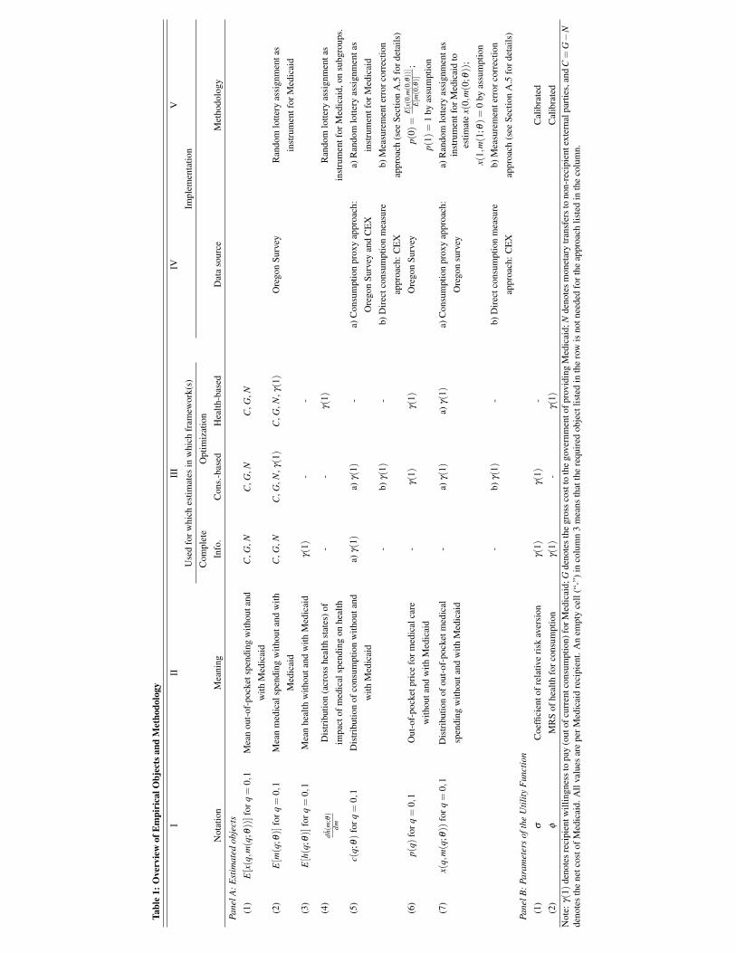
Tabl

e1:

Ove

rvie

wof

Em

piri

calO

bjec

tsan

dM

etho

dolo

gy

III

III

IVV

Use

dfo

rwhi

ches

timat

esin

whi

chfr

amew

ork(

s)Im

plem

enta

tion

Com

plet

eO

ptim

izat

ion

Not

atio

nM

eani

ngIn

fo.

Con

s.-b

ased

Hea

lth-b

ased

Dat

aso

urce

Met

hodo

logy

Pane

lA:E

stim

ated

obje

cts

(1)

E[x(q,m

(q; θ

))]

forq

=0,

1M

ean

out-

of-p

ocke

tspe

ndin

gw

ithou

tand

with

Med

icai

d

C,G

,NC

,G,N

C,G

,N

(2)

E[m(q

;θ)]

forq

=0,

1M

ean

med

ical

spen

ding

with

outa

ndw

ithM

edic

aid

C,G

,NC

,G,N

,γ(1)

C,G

,N,γ(1)

Ore

gon

Surv

eyR

ando

mlo

ttery

assi

gnm

enta

sin

stru

men

tfor

Med

icai

d(3

)E[h(q

;θ)]

forq

=0,

1M

ean

heal

thw

ithou

tand

with

Med

icai

dγ(

1)-

-

(4)

dh(m

; θ)

dmD

istr

ibut

ion

(acr

oss

heal

thst

ates

)of

impa

ctof

med

ical

spen

ding

onhe

alth

--

γ(1)

Ran

dom

lotte

ryas

sign

men

tas

inst

rum

entf

orM

edic

aid,

onsu

bgro

ups.

(5)

c(q;

θ)fo

rq=

0,1

Dis

trib

utio

nof

cons

umpt

ion

with

outa

ndw

ithM

edic

aid

a)γ(

1)a)

γ(1)

-a)

Con

sum

ptio

npr

oxy

appr

oach

:O

rego

nSu

rvey

and

CE

Xa)

Ran

dom

lotte

ryas

sign

men

tas

inst

rum

entf

orM

edic

aid

-b)

γ(1)

-b)

Dir

ectc

onsu

mpt

ion

mea

sure

appr

oach

:CE

Xb)

Mea

sure

men

terr

orco

rrec

tion

appr

oach

(see

Sect

ion

A.5

ford

etai

ls)

(6)

p(q)

forq

=0,

1O

ut-o

f-po

cket

pric

efo

rmed

ical

care

with

outa

ndw

ithM

edic

aid

-γ(

1)γ(

1)O

rego

nSu

rvey

p(0)

=E[x(0,m(0, θ))]

E[m(0,θ)]

;

p(1)

=1

byas

sum

ptio

n(7

)x(

q,m(q

;θ))

forq

=0,

1D

istr

ibut

ion

ofou

t-of

-poc

ketm

edic

alsp

endi

ngw

ithou

tand

with

Med

icai

d

-a)

γ(1)

a)γ(

1)a)

Con

sum

ptio

npr

oxy

appr

oach

:O

rego

nsu

rvey

a)R

ando

mlo

ttery

assi

gnm

enta

sin

stru

men

tfor

Med

icai

dto

estim

ate

x(0,

m(0

;θ))

;x(

1,m(1

;θ)=

0by

assu

mpt

ion

-b)

γ(1)

-b)

Dir

ectc

onsu

mpt

ion

mea

sure

appr

oach

:CE

Xb)

Mea

sure

men

terr

orco

rrec

tion

appr

oach

(see

Sect

ion

A.5

ford

etai

ls)

Pane

lB:P

aram

eter

sof

the

Util

ityF

unct

ion

(1)

σC

oeffi

cien

tofr

elat

ive

risk

aver

sion

γ(1)

γ(1)

-C

alib

rate

d(2

)ϕ

MR

Sof

heal

thfo

rcon

sum

ptio

nγ(

1)-

γ(1)

Cal

ibra

ted

Not

e:γ(

1)de

note

sre

cipi

entw

illin

gnes

sto

pay

(out

ofcu

rren

tcon

sum

ptio

n)fo

rMed

icai

d;G

deno

tes

the

gros

sco

stto

the

gove

rnm

ento

fpro

vidi

ngM

edic

aid;

Nde

note

sm

onet

ary

tran

sfer

sto

non-

reci

pien

text

erna

lpar

ties,

and

C=

G−

Nde

note

sth

ene

tcos

tofM

edic

aid.

All

valu

esar

epe

rMed

icai

dre

cipi

ent.

An

empt

yce

ll(“

-”)i

nco

lum

n3

mea

nsth

atth

ere

quir

edob

ject

liste

din

the

row

isno

tnee

ded

fort

heap

proa

chlis

ted

inth

eco

lum

n.

1

I II III IV

Full Sample

Treatment Compliers

(q=1)

Control Compliers

(q=0)Impact of Medicaid

Panel A: Oregon Data DemographicsShare female 0.60 0.57 0.60Share age 50-64 0.34 0.36 0.35Share age 19-49 0.66 0.64 0.65Share white 0.83 0.84 0.84Share black 0.03 0.03 0.03Share Spanish / Hispanic / Latino 0.11 0.07 0.08Mean family size, n 2.97 2.88 2.91

Panel B: Oregon Data Outcomes12-month medical spending, m Mean medical spending ($), E[m ] 2991 3600 2721 879 Fraction with positive medical spending, E[m >0] 0.74 0.79 0.72 0.07

12-month out-of-pocket spending, x Mean out-of-pocket spending ($), E[x ] 470 0 569 -569 Fraction with positive out-of-pocket spending, E[x>0] 0.38 0 0.56 -0.56

Health expressed in QALYs, E[h ] 0.77 0.78 0.74 0.05 Share in poor health (QALY=0.401) 0.11 0.10 0.17 -0.07 Share in fair health (QALY=0.707) 0.30 0.29 0.36 -0.07 Share in good health (QALY=0.841) 0.36 0.38 0.28 0.10 Share in very good health (QALY=0.931) 0.17 0.18 0.15 0.03 Share in excellent health (QALY=0.983) 0.05 0.05 0.04 0.02

Notes: This table reports data from a mail survey of participants in the Oregon Health Insurance Experiment (N=15,498). Columns II and III report the implied means for treatment and control compliers in the Oregon Health Insurance Experiment and column IV reports the estimated impact of Medicaid (i.e., the difference between Columns III and II). Since it cannot be directly observed whether any particular observation is a complier, the results in columns II and III are estimated using the IV techniques described in more detail in Appendix A2.1., as are the results in column IV. The Oregon health insurance lottery is used as an instrument for Medicaid coverage.

Table 2: Summary Statistics

I II III

Complete-InformationApproach

Consumption-Based (Consumption

Proxy)

Consumption-Based (CEX Consumption

Measure)

A. Recipient WTP for Medicaid, γ(1) 1675 1421 793 (standard error) (60) (180) (417)

Transfer component, T 569-863 661 661Pure-insurance component, I 812-1106 760 133

B. BenchmarksNet costs as fraction of gross cost, C/G 0.40 0.40 0.40Recipient WTP as fraction of net cost, γ (1)/C 1.16 0.98 0.55

Moral hazard cost, G-T-N 585-879 787 787

Notes: Estimates of WTP and moral hazard costs are expressed in dollars per year per Medicaid recipient. Standard errors are bootstrapped with 500 repetitions.

Optimization Approaches

Table 3: Willingness to Pay for Medicaid by Recipients