1

Compensation of a Manager:

The Case of Major League Baseball

Randy Silvers

Deakin University

70 Elgar Road

Burwood, VIC 3125 Australia.

Phone: 03 9251 7376

randolph.silvers@deakin.edu.au

and

Raul Susmel

Department of Finance

Bauer College of Business

University of Houston

Houston, TX, 77006

Phone: 713 743-4763

rsusmel@uh.edu

April 2014

Abstract

In this paper, we are interested in the informational value of Major League Baseball (MLB)

managerial compensation on a team’s performance. Using data on manager’s contracts, team

performance, and team and manager characteristics, first, we determine the variables that

influence a manager's salary. Then, we use a forecasting-type analysis to study the determinants

of a manager’s performance, measured by winning percentage, attendance or playoff

appearances. We find that a manager's past performance affects his current salary, but his current

salary does not affect the team's performance. Our results support the lack of a competitive and

efficient market for MLB managers.

.

2

1. Introduction

The wealth of reliable data and well-defined metrics make sports a fertile ground for testing

economic hypotheses. Sports organizations are largely similar to each other and operate in a

controlled environment on a regular basis. Each season is similar to the previous season.

Consequently, the effects of various competition rules, manager decisions, compensation

methods, and other policies can be elicited with confidence.

There is a vast literature exploring the compensation of managers, especially that of CEOs.

As pointed out by the survey of Frydman and Jenter (2010), the high level of CEO pay in the

U.S. spurred an intense debate about the nature of the compensation process and the outcomes it

produces. They report that the median compensation of CEOs increased in real terms by 6.3%

annually from 1992-2008. Interestingly, the median compensation of Major League Baseball

(MLB) managers in our sample increased, in real terms, by 6.8% annually from 1991-2013.

Even though the increase in MLB manager’s pay has also been large, there is a lack of papers

studying the determinants of MLB managerial compensation and the informational value of

managerial compensation on a team’s performance.

In this paper, we attempt to fill this gap. We are interested in the impact an MLB manager

has on a team’s outcome. Unlike the CEO compensation literature, where stock returns are taken

to be a measure of performance, there is no clear-cut measure to gauge the impact of a MLB

manager. Popular ways to measure a manager’s effect on a team’s performance include the

estimation of expected wins, using James’s (1986) “Pythagorean theorem,” as in Horowitz

(1994a, 1994b); estimation of a production function, as in Scully (1994); the estimation of the

impact on player’s performance, as in Bradbury (2006); the use of market salaries as in Kahn

(1993); and the analysis of the impact of a managerial change, as in Bradbury (2006). In this

paper, following Khan (1993), we rely on market salaries as a measure of productivity, since in a

competitive market the manager's salary equals the team's value of his productivity. In other

words, a manager's salary would be a sufficient statistic for this value.

Since salary information for MLB managers is scarce, we hand-collected from news reports

and internet websites a sample of 217 MLB managerial contracts from 1991-2013 with salary

information. We extended this sample to include an additional 169 managerial contracts, where

salary information was not reported. We match the contracts with several managerial variables,

team performance, and economic data, to form a dataset with over 40 potential explanatory

variables. Using a general-to-specific model selection approach, we first estimate the

determinants of a manager’s salary. As expected, we find that measures of a manager's

productivity, such as experience which proxies for human capital, and subjective measures of

performance which proxy for ability, as well as the team's market size, are significant

determinants of a manager's salary. Interestingly, James's (1986) Pythagorean expectation, “wins

over expectation” or WOE, has no significant effect on a manager’s salary. We also find that a

manager's network has a negative, if any, effect on his salary.

Then, using a forecasting-type regression, we turn to study different measures of

productivity. We find that the productivity of a manager, as measured by the team's winning

percentage, playoff appearances, or attendance, is not affected by the salary of a manager.

Rather, the determinants of a manager's productivity are largely the same as those of his salary,

3

notably, his experience and subjective measures of his performance. Again, WOE plays no role

in forecasting a manager's productivity.

Essentially, managers are compensated for past success via two channels: they gain

experience -- i.e., they are retained or hired by another team -- and they win awards. Importantly,

as in Mirabile and Witte (2012), we find that a manager's past performance influences his current

salary, but his current salary, which in efficient markets is a sufficient measure of his expected

productivity, is insignificant in predicting any of the three team performance metrics. Such a

disconnect renders relative salaries unreliable measures of relative productivities. The results are

consistent with a market characterized by extreme barriers to entry and human capital that is

relatively easily acquired; equilibrium then has an excess supply of managers who have

relatively similar ability.

The paper is organized as follows: Section I is the introduction. Section II discusses the

related literature review and models. Section III presents our simple model selection framework.

Section IV contains the description of the data and then the results and analysis. Finally, Section

V concludes.

II. Literature Review and Models

There are four broad categories of inputs that determine the productivity of a manager: his

effort, his ability, the other inputs, and the match quality. Given that it seems safe to regard effort

as inelastically supplied,1 the literature has measured the productivity of a manager by estimating

his ability and match quality, given the level of the inputs (player talent) that he can control.

There is no consensus measure of a manager’s productivity. Popular ways to measure a

manager’s effect on a team’s performance include the estimation of expected wins, using

James’s (1986) “Pythagorean theorem,” as in Horowitz (1994a, 1994b); estimation of a

production function, as in Porter and Scully (1982), Chapman and Southwick (1991), Scully

(1994) and Goff (2012); the estimation of the impact on player’s performance, as in Bradbury

(2006); the use of market or implied market salaries as in Kahn (1993), Ohkusa and Ohtake

(1994) and Orzag and Isreal (2009); and the analysis of the impact of a managerial change, as in

Bradbury (2006) and Hill (2009). The literature largely finds little differences between most

MLB managers, particularly those who have experience. This finding is common in other sports:

see, for example, (Fort et al. 2008) and Berri et al. (2009) for NBA coaches; Brown et al. (2007),

for football college coaches, Heuer et al. (2011) for German soccer, and Goff (2012) for several

sports.

Yet, even though managers, on average, have little effect on a team’s performance, managers

1 The absence of incentive-laden contracts and the public knowledge of the manager's decisions evince

that moral hazard is largely absent; career concerns and the desire for historic notoriety support the idea

that MLB managers' preferences are largely aligned with those of the general manager (GM) and owner.

Moreover, the well-defined and relatively narrow role of the manager implies that multi-tasking issues are

not of much consideration.

4

are frequently fired.2 Bradbury (2006) shows that MLB teams may fire a manager in order to

signal to their fan base that they are serious about winning, even if the team management knows

that replacement manager is no better than the replaced manager. If managers, especially

experienced managers, are largely equally productive, then even if this signaling effect is true,

there should be no difference in manager's compensation. Yet, some managers are paid

considerably more than others.

There is a vast literature exploring the determinants of CEO compensation. In general, the

main drivers are company size, company performance, human capital attributes of the CEO, and

industry effects--see the survey of Murphy (1999). However, likely due to the lack of

comprehensive salary information, there is a dearth of research into the determinants of

managerial salaries in sports. Grant et al. (2013) show that, in public schools, NCAA football

coaches are mainly compensated for past success (lifetime winning percentage) and size of

school.3

Mirabile and Witte (2012) find a similar result, NCAA football coaches are

compensated for past success; however, they also find that a coach's salary has no effect on a

team’s performance. This result is puzzling and may imply the existence of a market failure in

the sports market.

III. Salary Determination and Model Selection

Given the previous discussion, determining the true valuation of a manager to a particular

team in a particular year is not an easy task. There are three general categories that affect how

much a particular team values a particular manager: the manager's ability, the fit between the

team and the manager, which determine the productivity of the manager with that team, and the

value of the manager’s additional productivity for that team.

Regarding the first, we think of managerial ability as heterogeneous; at the onset of his

managerial career, the manager and all teams formulate a belief about his ability. Because

whatever factors are used to evaluate a manager's ability are public, and because the manager

himself does not have any experience or expertise, this belief is the same for the manager and

each team. As he gains experience, the precision of the belief increases. We can think of the

belief together with the precision as an assessment of his ability.

Regarding the second, the quality of the match can vary. Some managers are assessed to

work well with young and inexperienced players and develop their talent, others are assessed to

handle superstars who have egos, and others, as evidenced by the number who are promoted

from within the organization, are familiar with the goals and ethos of the team.

2 During our sample period 1990-2013, we observed 80 firings during 672 manager-years, including 40

during a season and 10 before a season had begun. The median tenure for a manager is 2.63 years.

3 In the linear compensation formulation, they also find that in-season rank (BCS rank) is significant at

the 5% level.

5

Lastly, MLB, as with other U.S. sports, is a legalized cartel. Entry is rare and restricted, with

new entrants often having to directly compensate the existing teams, and being unable to freely

locate. Existing teams face similar restrictions on changing their location.4 Consequently, teams

cannot choose, a la Hotelling, their location and thereby move to an area where additional wins

and playoff appearances would generate more additional revenue than in their current location.

Another almost immutable team characteristic is its history, which may influence the actual size

of the market.

Thus, it is not clear which variables should be included in an MLB manager's salary

equation. We expect measures that are correlated with a manager's ability and with the precision

of that belief, such as number of seasons as a manager; measures of fitness such as a connection

to the team or GM; and measures related to the team's valuation of productivity, such as the

market size of the team, to all significantly affect MLB manager's salaries. That is,

Salary = f(assessment of manager’s ability, fitness, team’s valuation of productivity, other

variables) + error term

Because a manager is a sui generis job for which other positions, such as MLB coach or

minor league manager, may not be a good predictors of ability as a manager, it is worthwhile

distinguishing those managers with MLB managing experience from those with none (rookies).

Additionally, the contracting situation is fundamentally different between renegotiating with, or

extending the contract of the current manager, versus signing a new manager (new hires).5

As mentioned above, the richness of sports data makes the choice of independent variables

complicated. There are many potential variables that can be used to assess a manager’s ability:

years of managerial experience, age, manager’s lifetime winning percentage, manager’s lifetime

number of winning seasons, manager’s lifetime playoff record, number of times a manager was

voted among the top five for the Manager of the Year (MOY) award, etc. We have 15 variables

that a GM can use to assess a manager's ability, which should explain much of a manager’s

salary. Given the breadth of the data, it is not surprising to see that different papers use different

explanatory variables. For example, to measure past managing success, Khan (1993) and

Mirabile and Witte (2012) both use the manager's past winning percentage at the time of his

hiring; however, the former uses the manager's entire history, the latter uses only the previous

five years. A similar difficulty arises when deciding which variables to include to measure

4 During our sample period 1990-2013, only one team of the 26 moved; there were no public threats to

move. Twice, two teams entered MLB. Given the remarkable increase in mean team valuation, free entry

would have induced several more entrants.

5 Similarly, some firms hire CEOs from without, others promote from within; additionally, the

accomplishments of rookie CEOs before their promotion are imperfect predictors of ability as a CEO.

One important difference is the presence of moral hazard within firms, so that the potential to become a

CEO motivates other senior managers, aligning their actions with those of ownership.

6

fitness and a team's valuation of productivity. Overall, our data set contains more than 50

potential independent regressors (see Appendix for a list of all the variables available).

To select the best model, we follow a general-to-specific method, see Campos et al., (2005).

After some F-testing reductions, using a 10% significance level to drop variables, we have a final

model. Given that many variables are highly correlated, we check two multicollinearity

indicators: VIF and Condition Index. We follow the usual rules of thumb to determine if

multicollinearity is a problem; that is, VIF > 5 and/or Condition index > 10 --see Belsley (1991).

If these rules of thumb are violated, we remove the variables that we suspect cause collinearity.

A word about the dating of the data used in the estimation of the salary equation: Taking the

time index t to demarcate the end of the season, a manager’s and players’ salaries are determined

as of the start of the next season; that is, they are variables dated t-1. A team’s GM estimates the

expected productivity of a manager (and players) based on information available at t-1 –i.e., at

the end of the previous season. Additionally, some managers sign multi-year contracts so that the

salary in season t was set after season t-2 or t-3. We follow this convention to estimate a salary;

that is, we only consider as potential explanatory variables for salary for season t, variables that

are dated up to the contracting date. This approach is also used by Mirabile and Witte (2012).

IV. Data

We consider all MLB managers from 1991 onward who were hired by a team. Unlike for

players, and for CEOs of public corporations, there is neither a single reliable source for MLB

manager salaries nor are they consistently reported. Some teams routinely disclose manager’s

salaries, while others seldom do it. Additionally, a manager’s agent may leak the information to

the press, likely as a marketing tool, and sometimes, after a manager is fired, the value of the

remaining years in the contract is reported by the press. It is rare to see the publication of the

complete distribution of MLB managerial salaries for one specific year. One of the few

published salary distributions by Sports Illustrated for the year 1987 is used by Khan (1993). He

relies on the 1987 Sports Illustrated dataset, also mentioned in Chapman and Southwick (1991),

to estimate market salaries from 1969-1987. For this paper, we hand-collected salaries and

contract duration from newspapers and internet websites. Our starting point was the Baseball

Prospectus Cot's Baseball Salaries website.6 Then, we checked managing hiring and firing

announcements from local and national newspapers, which usually cited AP reports, along with

several other websites.

We were able to collect 217 manager-contracts with salary information. Bonuses and

incentives are, in general, not available. That is, we are forced to focus on a manager’s base

salary compensation. As previously discussed, this is not likely problematic due to the absence of

moral hazard. Given that contracts are, in general, reported as an aggregate number for the total

duration of the contract, we focus on the contract’s annual average salary.

6 See http://www.baseballprospectus.com/compensation/cots/

7

We augment our data with an additional 169 manager-contracts, without salary information,

for a total of 386 contracts. Of the 386 contracts, 172 are for newly hired managers and 214 are

extensions or renegotiations. Of the 172 contracts for newly hired manages, three have no

disclosed duration and 86 were rookies. Ten newly hired managers appear in our dataset more

than once, forming what the baseball sports writers call "the musical chairs" group. Also, of the

217 manager-contracts with salary information, 99 are for newly hired managers. There is at

least one observation for each of the 30 teams. Only two managers were hired from another team

while they were still under contract with an existing team.

Managers' and teams' stats, payrolls and attendances are taken from Baseball Reference

(www.baseball-reference.com) and The Baseball Cube (www.thebaseballcube.com). Annual

team valuation, revenue, and operating income information are taken from Forbes annual

baseball valuation study, usually reported in April. Table 1 presents the distribution of annual

mean manager salaries, along with the annual means of team valuation, team revenue, and player

salary. Table 1 shows a large increase in manager’s salaries, with the mean growing at an

average annual rate of 9.7% from 1991-2013. This annual increase in managerial salaries is

slightly higher than the average annual increase in team’s mean valuations (8.6%), revenues

(6.9%) and payroll (7.8%) over our sample.

IV.1 Descriptive Statistics

Table 2 provides characteristics of the data. The second column describes the characteristics

of all the manager-contracts in the sample, while the third column describes the characteristics of

the new hires. Around 70% of the newly hired managers have previous managerial experience in

the minor leagues. Fourteen newly hired managers were initially hired as interim managers. The

average initial contract duration for all managers is 2.00 seasons, while for new managers is 2.41

seasons; however, on average, a manager only serves a little bit more than 80% of the duration of

the contract. Overall, 25% of all managers and 30% of all newly hired managers are fired. The

catcher position is over-represented, more that 30% of the managers were catchers as a players.7

Table 3 provides the descriptive statistics for both the 217 contracts with salary information,

and the contract duration for all 383 contracts. Table 3 also contains some descriptive statistics of

the managers' experience and the teams.

Consistent with the theory, on average, non-rookie newly hired managers make significantly

more (142%) than newly hired rookie managers. A non-rookie newly hired manager is paid a

competitive salary, similar to the average contract of all contracts in the sample. Also,

7 This contrasts with approximately 10% of a team's active roster as being a catcher. Moreover, catchers,

like pitchers and First Basemen, rarely play multiple positions, though some move to First Base later in

their careers. Other position players do play in multiple positions, and some do play First Base, but only

injuries and ejections prompt a manager to play a non-catcher as a catcher.

8

experienced –i.e., non-rookie– new hires have a significantly longer duration for their initial

contract, longer than the duration of the average contract, which may be the result that many

well-established older managers, such as Jim Leyland or Bobby Cox, at the end of their

managing careers work with very short contracts.

Experienced new managers are significantly older than rookie managers (55 years old vs 46

years old) and tend to have managed more time in the Minor League system (4.85 seasons vs.

4.35 seasons). Teams with higher payroll and higher attendance tend to hire non-rookie

managers.

Looking at the team data, we find that new managers are hired by teams with losing records,

as expected. Teams with higher value, payroll and attendance --likely teams in larger markets--

tend to hire new managers with experience. Payroll and attendance have grown over the past 30

years. But, not surprising, new managers are brought to teams that had a negative change in

attendance and a lower than average increase in payroll during the season prior to the new

appointment.

Table 4 presents some statistics that describe the change in the team's performance and

outcomes during the first full season a new manager is hired. We look at the changes in: team

performance variables -- winning percentage, total runs scored, and total runs against; player

characteristics --average batting and pitching ages; and team characteristics –franchise value and

attendance. We also look at a team’s wins-over-expectation (WOE), defined by James (1986);

this is a commonly used indicator of managerial performance --see, Horowitz (1994a). Under the

WOE measure, expected win-loss percentage is measured using the Pythagorean expectation --

i.e., expected win-loss percentage in a season are equal to the square of total runs scored in that

season, divided by the sum of the squares of the total runs scored and total runs allowed.8

The simple correlations indicate that a new manager increases the winning percentage,

increases runs scored and decreases runs against. However, none of these changes is statistically

significant. The lack of a significant immediate impact of a new manager is consistent with the

findings in Bradbury (2006). We also compare the effects of new managers, distinguishing

between rookies and experienced managers. Each of the effects of rookies versus experienced

managers in their first full season is statistically insignificantly different from each other, and

from zero, with one exception, WOE. Whereas an experienced manager’s change in WOE is

positive but insignificant (0.38 wins over expectation), a rookie manager’s change in WOE is

negative and significant (-1.1 wins over expectation); nevertheless, this difference becomes

statistically insignificant during the second full season, indicating a quick learning curve.

We also tend to see a lower than average change in franchise value and attendance for

8 Under the assumption that runs scored follow an independent Weibull distribution, Miller (2007) derives

the Pythagorean Expectation formula for wins. Davenport and Woolner (1999) argue for a Pythagorean

exponent of 1.86.

9

franchises that hire new managers. These are not too surprising since a vast majority of hires of

new managers follow seasons of poor absolute performance and poor attendance. But, again, the

changes are not statistically significant.

Given the potential for multicollinearity in some of the variables, we also rely in factor

analysis to try to reduce the number of variables use. We divide some of the variables into two

groups: 11 variables are designated as part of a managerial group and 12 variables are designated

as part of a team’s characteristic group.

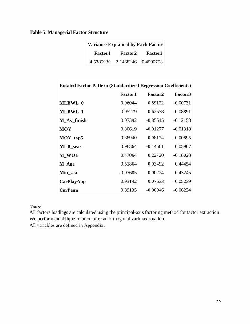
For the management group, we were able to find a clear, three-factor structure.

Unfortunately, for the team’s characteristic group, we were not able to find a clear factor

structure. The three managerial factors are defined in Table 5. The first factor, MF1, is heavily

influenced by variables that can be interpreted as indicators of a manager's ability and the

precision of that belief (MOY, MOY_top5, number of MLB seasons as a manager and career

playoff appearance and pennants won); the second factor, MF2, loads mainly on past season's

performance, as measured by winning percentage and divisional finish; and the third factor,

MF3, mainly loads on a manager's age and the number of seasons managed in the minor leagues.

Since we are particularly interested in analyzing the role of WOE, we recreate the first factor

MF1 by imposing the factor loading for WOE to be equal to zero. We call this reformulated

factor MF1_WOE.

IV.2 Estimation of Salary Equation

In this section, we estimate salary equations for baseball managers. For each, we estimate a

salary equation following the general-to-specific method discussed in Section III. As usual in the

labor literature, we use as the dependent variable log annual salary. We estimate salary equations

for all managers, for all experienced managers, and for all new hires.

Theoretically, we expect that variables that measure a manager's ability also affect a

manager's salary. Note that some of these measures are subjective, for example winning a

Manager of the Year Award, used by Hill (2009) and some measures are objective, for example,

a manager’s WOE, used by Horwitz (1994a).

We also expect that variables that make this belief more precise will affect a manager's

salary. For example, consider two managers who have the same WOE or winning percentage but

differ in their experience. The belief about the manager's ability is increasing in this experience.

Moreover, survivorship bias implies that managers about whom the assessment is low, are not re-

signed or re-hired. Lastly, remuneration for more experience is consistent with the acquisition of

human capital, particularly general human capital.

In the second column of Table 6, we report the results for log salaries. The general-to-

specific approach produces eight explanatory variables, with an R2 equal to .82. The results

largely confirm intuition regarding the role of measures of quality and experience. The number

of years as an MLB manager (MLB_seas) and winning and being voted in the top 5 of the MOY

award are significant at the 5% level.

10

The results also echo a similar result in the CEO compensation literature. Much as CEOs

who receive awards subsequently realize greater compensation (see Malmendier and Tate, 2009),

both winning (Award) and finishing in the top five of MOY balloting (Aw_top5), at least once,

result in the manager receiving a larger salary. Interestingly, the number of seasons for which a

manager finished in the top five of the MOY balloting (MOY_top5) is also significant, which

may indicate the presence of some non-linear effects of the MOY vote on salary.

There is one other variable related to the assessment of a manager that is significant, the

number of seasons he managed in the minor leagues. Perhaps more interesting is its significance

and negative sign. This could reflect the presence of private information or the acquisition of

firm-specific human capital, both of which would seem to reduce his bargaining power, or the

manager's career concerns. Although much information is public to the manager and all teams,

some information, especially for those who were minor league managers is private to the

manager and the particular team. Alternatively, having managed in the minor league system of a

team is consistent with the acquisition of firm-specific human capital, which makes the manager

less valuable to other teams. Additionally, a minor league manager may be willing to accept a

lower salary than otherwise in order to enhance his prospects of becoming an MLB manager,

particularly if there is an implicit contract of progressing to the major league level where their

ability becomes learned.

Aside from the manager's age, which is only selected in the log salary regression where it is

only significant at the 5% level, there are two variables related to the team's valuation of

productivity, a time trend and the log of payroll. The other variables related to a manager’s

ability ia the square of his age. However, this is only selected in the log salary regression and is

only significant at the 10% level.

The time trend is highly significant, which is expected given the trend shown in Graph 1 and

Table 1. Casual observation of the growth of baseball franchise values indicates that managers

have reaped some of the gains in popularity and consumer expenditures. A time trend though

applies uniformly.

So-called large-market teams have larger payrolls and, as discussed above, place a higher

value on the productivity of a manager. Moreover, during our sample period, their payrolls have

increased much more rapidly than those of the remaining teams. Payroll (in logs) also enters the

log salary regression with a positive sign.

As Table 1 and Graph 1 clearly show, managerial salaries have increased over time. Given

this feature of the salary data and the fact that nominal variables seem correlated with a team’s

size, in order to check the robustness our estimation, we also estimate the manager's salary

standardized by the team’s payroll. The results of this estimation are in the third column of Table

6. The reduction in the R2 to .5152, is likely due to the lack of a time trend to explain the log of

the ratio of a manager’s salary to a team’s payroll. Nevertheless, overall, the signs and

magnitudes of the coefficients of the managerial variables are similar to those reported for log

11

salaries. This is not a surprising result, given that managerial variables are not expected to be

correlated with a team’s payroll. The time trend is also not significant, which is to be expected

given the standarization used. Instead of team’s payroll, change in payroll (Dpay) appears in the

regression, though it is not significant.

There is one additional explanatory variable in the log salary payroll-standardized regression,

the team's winning percentage in the previous season, which is significant and negative. That is,

a higher winning percentage in the previous season is correlated with a lower manager salary

relative to team’s payroll. Thus, assuming that as a team’s winning percentage increases, so does

a team’s revenue, it seems that a team’s payroll increases more (less) than a manager’s salary

when a team is winning (losing). This indicates that payroll is more sensitive to past team

performance than is a manager’s salary.

Since we are particularly interested in the effect of the managing specific variables on salary,

we run many specification tests of the selected models. We perform several LM tests to check

for the inclusion of a manager's previous winning percentage, number of winning seasons, other

manager factors as determined by factor analysis, and a manager’s lifetime WOE. None of these

tests is significant at the usual significance levels. In particular, Horowitz’s (1994a) WOE plays

no role in the determination of a manager’s salary--an LM test for the inclusion of a manager’s

WOE has a value of 0.9328, which is not significant at the usual significance levels. That is, the

evidence suggests that the general managers, who hire the managers, assess the abilities and

productivites of managers using the more subjective metrics such as winning awards, not,

directly or implicitly, objective metrics.

Much of the previous analysis suggests that the determinants of a manager's salary may differ

depending upon whether the team is re-signing or extending the contract of its current manager,

or hiring a new manager who has experience. These differences reflect the differences in

bargaining power.

IV.2.1 Experienced and New Hired Managers

Given that the determinants of extending or renegotiating a contract may be different from

the determinants of hiring a new manager, which may differ from hiring a rookie manager, we

estimate two separate salary equations: one for all experienced managers and one for all

experienced. Table 7 presents the results for log salary of experienced MLB managers.

For the salary equation for all experienced managers, the results are shown in the second

column of Table 7. The general-to-specific process selects 10 explanatory variables with an R2

equal to .8059. The managerial variables selected are the same as in Table 6: minor league

seasons (Min_sea), finishing in the top five of the MOY vote (MOY_top5), MLB seasons as a

manager, and the dummy variables for winning at least one MOY (Award) and for finishing at

least once in the top five of the MOY vote (Aw_Top5).

Rather than team payroll, change in payroll (Dpay) is selected in the regression/survives the

model selection method. A team characteristic variable is also selected: age of the batting lineup

12

at (or season) t-1 (Bage_1). The matching hypothesis may explain the effect of a team’s age on a

manager's salary. Consider a team that is successful. The GM is likely to retain many of the same

personnel, including the manager, who now has a stronger assessment and, perhaps, a better

fitness with that team. The player personnel, largely unchanged, is also older.

A network variable (Interim) is selected in the model, showing up with a negative effect on

salaries. A large percentage of the firings or separations (50% or 40 out of 80 in our sample

period) occurred during the season; the individual who assumed the role of manager for the

remainder of the season was sometimes subsequently re-hired. Half of these managers (Interim)

had previous MLB managerial experience. The coefficient on this Interim variable is negative,

probably reflecting a lack of alternatives or “limited choices,” as described in Loury (2006).

Our final salary regression is for experienced managers who are new hires; the sample size

(95) is smaller. The results of the general-to-specific approach are presented in the last column of

Table 7. The model selection strategy selects similar managerial assessment variables, except

that MOY_top5 is removed because it causes multicollinearity. The age of the batting lineup,

change in payroll and the dummy variable Aw_top5 are not selected by the general-to-specific

model selection strategy. A network variable, having a previous relation to the team’s GM

(Connection), is also selected, again with a negative sign, but it is not statistically significant at

the 5% level. Overall, the signs are the same for all experienced managers, but some coefficients

are larger (MLB_seas and Award), likely picking up the effect of the variables excluded

(MOY_top5 and Aw_top5, respectively).

Again, we check the model specification with a set of LM tests. We test for the inclusion of a

manager’s WOE (LM-M_WOE); a manager’s previous winning percentage (LM-M_WL); three

managerial factors as determined by common factor analysis (LM-M-Factors); and three

variables that describe a team’s previous record: runs scored, runs against, and team’s winning

percentage at t-1 (LM-Team Rec). None of these tests is significant at the usual significance

levels.

Overall, we find that MLB manager salaries are positively affected by very simple

managerial measures that reflect past perceived good performance in the form of awards (MOY

votes). Experience as a manager also plays a role; the number of seasons as an MLB coach

(manager?) has a positive effect on managerial salary, whereas the number of seasons as a minor

league manager has a negative effect on managerial salary. Market size, in the form of payroll,

also has a positive effect on a manager’s salary, a similar result to the CEO compensation

literature, where company size is a main determinant of CEO compensation--see Rosen (1982)

and Kostiuk (1990).

If the path to becoming an MLB manager resulted in a lower salaries by being a minor league

manager than not, we would not expect individuals to choose this path. However, the barriers to

entry of new teams restricts the quantity of MLB coaching positions so that many would-be

MLB managers believe that becoming a minor league manager is the best path available to

becoming a a major league manager. Additionally, it is likely that being a minor league manager

13

results in greater probability of becoming an MLB manager than does being a major league

coach. This lack of entry highlights a key difference with the market for CEOs, and one that may

be a source of the market inefficiency.

IV.3 Managing and Winning Percentage

We have shown that measures of managerial ability are significant factors that explain a

manager's salary --i.e., past successful performance may imply greater ability, which increases a

manager's salary. We now, in a sense, reverse the forecasting exercise. If better managers are

remunerated more, then their ability ought to manifest itself through superior performance.

As pointed out by Khan (1993), in a competitive market, salaries represent the marginal

productivity of a manager. Moreover, a manager’s salary should be a sufficient statistic of a

manager's productivity --i.e., all other indicators of managerial ability and precision, as well as

fitness, should be subsumed into the market salary. Thus, we expect both a positive correlation

between a manager’s salary and a team’s winning percentage, and all other managerial variables,

including years of experience and manager’s WOE, to be uncorrelated with a team's winning

percentage.

Winning percentage is, of course, not only determined by managerial skills, but also by other

factors, including players’ performance and luck. In general, players’ performance during the

season can be influenced by managerial decisions. Thus, including in a regression measures of

managerial ability and players’ performance will create simultaneity problems.9

To avoid this problem, we take a slightly different approach from the one taken in Khan

(1993). Since salaries for managers and players are determined before the start of the season, but

winning percentage is determined at the end of the season, estimating a regression relating a

manager’s salary to the ex-post winning percentage of a team is similar to estimating a

forecasting equation. That is, we try to determine if a manager’s salary, determined before the

start of season t, can be used to explain the winning percentage at the end of the season t.

However, there are many potential variables that can be used to forecast winning percentage at t.

Again, we start by using a general-to-specific model selection approach to determine the

explanatory variables. In addition to the managerial and team variables employed to determine a

manager's salary, we include the manager's log salary. All variables used to predict a team's

winning percentage in t are those t-1 variables. We also included a dummy for whether the

manager was a new hire or not, and a dummy for whether the manager had signed an extension

prior to t. In order to be parsimonious and to reduce potential collinearity, we include as potential

explanatory variables the three managerial common factors as determined by factor analysis.

Then, we perform a series of LM tests to check the specification of the model.

9 Many previous studies that assessed the managerial ability using the "Pythagorean theorem" suffer from

this same criticism--they use the current season's runs scored and runs against variables as exogenous

regressors to formulate an expected winning percentage and then compare the actual winning percentage.

14

We estimate three forecasting equations: one for the winning percentage during the first

season of a manager’s contract (T_WL_0), another one for the second season of a manager’s

contract (T_WL+1); and the last one for the average of the first two seasons of a manager’s

contract (T_WL_av). We only consider the winning percentage at t and at t+1, since the mean

duration of a manager’s contract is two years.

Table 8 shows the results for winning percentage during the first season, the second season,

and the average of the first two seasons of a manager’s contract. The main drivers at t-1 are the

modified first managerial factor (MF1_WOE), change in payroll, and previous season winning

percentage. All of these variables enter with a positive impact on winning percentage.

MF1_WOE measures managerial ability and precision; importantly, it includes variables that

previous studies have not considered, namely, having made the playoffs and playoff

performance. We do not dispute that win-maximization is a major objective of teams, and of

managers; rather, having made the playoffs and having achieved success therein, are additional

factors for which managers are compensated. It could be that these factors lead to an updated

assessment of the manager that is stronger, or give the manager more bargaining power,

especially considering a loss of fan support for a team that fires or fails to re-sign a manager

whose team made the playoffs and was successful.

For the first season's winning percentage, a manager who was a catcher performed

significantly better (two more wins out of 162) though this dummy is only significant at the 10%

level. However for the second season, this variable disappears as an explanatory variable,

indicating that whatever human capital that a player who had been a major league catcher as a

player had, was acquired with one year of MLB managing experience. To the extent that this is

true, that having been a major league catcher affords an understanding of the game superior to

having been a pitcher or another position player, it is also consistent with the over-representation

of former major league catchers as MLB managers.

For the second season's winning percentage, a different variable, the age of the batting lineup

(Bage_1), survives the model selection process --a team with an older position-player roster is

expected to have a lower winning percentage. However, the effect is only significant at the 10%

level and economically small (one less win out of 162) for a team that is one year older. It could

be that a team that has had success, retains more of its roster, ages, and either regresses to the

mean or incurs more injuries, which are often age-related.

Five LM specification tests are reported in the bottom of Table 8. We test for the inclusion of

a manager’s WOE; a manager’s previous lifetime and previous season winning percentage; log

salary; log salary scaled by payroll; and other managerial factors. None of the LM tests is

significant. In particular, the LM-log Pay and LM_log Pay_P, confirm the findings in Orszag and

Israel (2009), Zimbalist (2010), and Mirabile and Witte (2012), where they were unable to find

evidence that salaries had a positive and significant impact on winning percentage. A similar

result appears in the recent CEO compensation literature. Cooper at al. (2013) find that CEO pay

15

is negatively related to future stock returns for periods of up to 3 years, with the higher paid CEO

having a more negative impact on future stock returns..

IV.4 Managing and Playoffs

It can be argued that good teams are willing to pay, not just for regular season performance,

but for making the playoffs. Making the playoffs brings significant extra revenue to a team.10

Thus, a winning percentage per se may not be the relevant metric of marginal productivity for

managers who are hired by teams expected to go to the playoffs.

In order to test this potential non-linearity in the relation between a team’s performance and a

manager's productivity, as measured by salary, we estimate a probit model (where 1=team makes

the playoffs) using maximum likelihood. As before, we estimate the probability of making the

playoffs in t with information available at t-1 and use the same general-to-specific approach to

select from 40 potential explanatory variables. Since we also want to reduce the potential for

multicollinearity, we try to be as parsimonious as possible. We use a 7.5% significance level in

the model selection strategy, instead of the previous 10% level.

Table 9 shows the results of the probit estimation. There are only three explanatory variables

that survive the general-to-specific selection method: years of experience as an MLB manager,

appearing in the playoffs the previous season (Playoff_1), and the previous season’s winning

percentage.

We run several specification tests; in particular we check if a salary variable (log salary or

log salary scaled by team’s payroll) should be included in the final model. A Wald test strongly

rejects the inclusion of salary information in the probit model. We also reject the inclusion in the

final model of several other variables: the ability variables--manager’s WOE, manager’s lifetime

winning percentage, MOY, MOY_top5, and rookie dummy--the age of the batting lineup, and

the connection dummy. That is, neither the manager's salary nor the various managerial

variables, especially those related to ability and match quality, that affect his salary, have any

effect on the probability that the manager's team makes the playoffs.

IV.5 Managing and Attendance

Bradbury (2006) argues that firing a manager following poor results may be seen as a

positive signal by the fans. He finds that attendance increases immediately after the firing of a

manager. It is possible that firing a manager has no effect on winning percentage. Nevertheless,

it may increase a team’s revenue by increasing attendance, which is a major component of local

revenues, which themselves comprise nearly 80% of a team’s revenue –see, Levin et al. (2000).

The cost of firing a manager is relatively minor: the compensation to the newly hired manager

that covers the fired manager's remaining contract term, and the opportunity cost of the GM's

time.

10 See article in Fangraphs.com, “Estimating Postseason Revenue For Players And Teams,” by Wendy Thurm,

November 2, 1012. 2ttp://www.fangraphs.com/blogs/estimating-postseason-revenue-for-players-and-teams/

16

Previous studies of sports attendance find that many factors play a role in team’s attendance:

a city’s weather, month, day of the week, a team’s location, lagged team’s performance,

promotions, strikes, etc. Briefly, positive and significant effects have been found for: a team’s

current and previous season's performance, see Scully (1974), McDonald and Rascher (2000),

and Zygmont and Leadley (2005), among many others; the market size (income and population),

see Winfree et al. (2004); National League, see McDonald and Rascher (2000); and higher

opening day payroll, see Barilla et al. (2008). Additionally, annual attendance is found to be

highly autocorrelated, see Barilla et al. (2008).

In this section, we attempt to measure the effect of an MLB manager on annual (log)

attendance. We follow the general-to-specific model selection strategy used in the previous

sections, we select the determinants, known at the start of the season (t-1 variables), of time t

attendance.

Table 10, in the second column, shows the results for log attendance. Given the strong

autocorrelation of attendance, we also present in the third column, the results for changes in

attendance. Consistent with the papers cited above, we find that a National League dummy, runs

scored, a team’s change in payroll, making the playoffs, and previous attendance can be used to

forecast attendance. In addition, all of these variables have a positive effect on the forecast of

next season’s attendance.11

We also find that a managerial variable, namely, experience has a

positive effect on the forecast of next season’s attendance.

We perform several specification tests for the inclusion of several variables in the forecasting

of attendance. We test for the inclusion of a manager’s lifetime WOE, lifetime winning

percentage, current salary, rookie status, and the MOY votes, as well as our three managerial

factors, and a manager’s network (connection, interim status, promotion from within); we also

test for the team’s age, payroll, previous runs against, and previous and current winning

percentage. All these tests cannot reject the hypothesis that these variables does not belong in the

forecasting equation of a team’s attendance. In particular, we find that a manager’s salary seems

to plays no role in attendance. Finally, in the spirit of Bradbury (2006), we test if a new manager

(New Hire variable) plays a role in annual attendance. The last LM (LM_New_Hire) tests this

hypothesis. Again, we find no support for the inclusion of a dummy for a change in managing in

the forecast of next season’s attendance.

IV.6 Managing and Experience: Discussion The experience of a manager, measured in seasons managed at the MLB level, has a positive

and significant effect on a manager’s salary as well as on forecasting winning percentage,

playoff appearances and attendance. It is puzzling that experience, though priced in the

determination of a manager’s salary, plays a more important role than other variables that

11 Attendance is strongly correlated, with an AR(1) coefficient of .755, but it is not an I(1), as the negative

coefficient and t-stats (DF test) in the regression in changes shows.

17

measure the manager’s productivity. In this sense, it seems that teams think of experience as a

sufficient statistic for a manager’s productivity. However, we generally think of experience as

possibly signaling inherent ability and, possibly, the acquisition of human capital; that the more

direct measures of ability and productivity seem not to forecast performance is puzzling.

In order to understand the role of experience, we study the joint distribution of experience

with several team and managerial variables. Table 11 shows this joint distribution, dividing

experience into four categories: “Rookie,” “Less than 5 years,” “Between 5 to 9 years,” and

“More than 9 years.” A bold number indicates statistically significantly difference from the

corresponding value in the preceding column. We find that those managers who survive and

accumulate more seasons, have a higher lifetime winning percentage, a higher WOE (lifetime

and per season), and higher likelihoods of having both won awards and made the playoffs. Thus,

experience, especially in the last group, is correlated with all the variables teams are likely to

associate with a manager’s productivity.

It is perhaps surprising the lack of support for a manager’s lifetime WOE as a measure of a

manager’s salary and especially productivity; after all, lifetime winning percentage and lifetime

WOE are highly correlated in the unconditional distribution. In an unconditional analysis,

Horowitz (1994a, 1994b) strongly argues for the use of WOE as a measure of a manager’s

performance, with the caveat that his analysis uses managers that have managed for at least 10

seasons. Our analysis is slightly different in the sense that we do have a conditional model and

our sample is not restricted to the most-experienced managers. Our results show that the

inclusion of other variables that measure productivity and experience renders WOE entirely

uninformative for forecasting productivity.

Not surprisingly, managers who gain experience realize greater salary; e.g., the average

salary for a manager with more than nine years of experience is $1.5 million (242%) more than

that for a manager with less than five years of experience. That is, unconditionally, experience is

positively correlated with lifetime winning percentage, which itself is positively correlated with

salary; yet, surprisingly, in the conditional regression framework this correlation disappears.

Some managers moved into that role from being a minor league manager, a path that resulted

in a lower salary than managers who entered from elsewhere. Yet, interestingly, the most

experienced managers who did manage in the minor leagues, had a significantly higher winning

percentage. This may reflect the fact that managers who do very well in the minors are identified

and promoted quickly to the majors,. As a result of this quick promotion, they accumulate more

MLB managerial experience than those MLB managers with longer stays in the minors. It is also

possible that a very successful short stint in the minors signals superior ability, which is reflected

in better performance realizations, renewed employment, and higher salaries.

Lastly, we note that many experienced managers do move to other teams, often voluntarily.

More-experienced managers work for teams with greater value, higher attendance, and higher

quality, as proxied by payroll and past winning percentage. The positive correlation between

18

experience and these team variables may be evidence of efficient matching, where the most

productive managers are paired with the teams that have the highest value of productivity.12

V. Conclusions

In this paper, we first estimate salary equations for MLB managers. Overall, we find that

MLB managing salaries are positively affected by very simple managerial measures that reflect

past perceived good performance (notably, voting for the Manager of the Year). The number of

MLB seasons managed has a positive effect on salaries, but the number of minor league seasons

as a manager has a negative effect on salaries. Size, through team's payroll, also is a driver of

MLB manager salaries. For the whole sample, a manager’s network has a negative, but

insignificant impact on a manager's salary.

We then test if a manager's salary is a predictor of a team's performance. We found/find

that a manager's current salary has no impact on that season's winning percentage, attendance, or

playoff appearance; moreover, a manager's previous performance, measured as past winning

percentage and lifetime WOE, has no effect on a team's performance. The lack of a relation

between a manager’s salary and a team’s performance is an indicator of market inefficiency.

Our results suggest that the market for MLB managers is neither competitive nor

efficient. In perfectly competitive labor markets with complete information, a worker is paid her

marginal revenue product; relative wages reflect relative productivities. As with the market for

CEOs, there is a disconnection between a manager's salary and his expected productivity. This

situation may reflect the characteristics of the market for MLB managers where monopsony

power and the value of signaling to fans a commitment to winning can distort salaries.

12 We make this statement with extreme caution. Several large-market, high payroll, and

successful teams have recently replaced extremely experienced managers with rookies or

inexperienced managers--notably, New York Yankees (2008), Los Angeles Dodgers (2011), St.

Louis Cardinals (2013), Detroit Tigers (2014).

19

References

Barilla, A. G., K. Gruben, and W. Levenier (2008), “The Effect Of Promotions On Attendance

At Major League Baseball Games”, The Journal of Applied Business Research, Third Quarter,

Volume 24, Number 3.

Belsley, D. A. (1991 ). Collinearity diagnostics: Collinearity and weak data in regression. New

York: John Wiley & Sons.

Berri, David J., Michael A. Leeds, Eva Marikova Leeds, and Michael Mondello (2009), "The

Role of Managers in Team Performance," International Journal of Sport Finance (4) 75-93.

Bradbury, J. C. (2006), “Hired to Be Fired: The Publicity Value of Managers,” unpublished

manuscript, Kennesaw State University.

Brown, Todd, Kathleen A. Farrell and Thomas Zorn (2007), "Performance Measurement &

Matching: The Market for Football Coaches," Quarterly Journal of Business and Economics (46)

21-35.

Campos, J., N. R. Ericsson and D. F. Hendry (2005), “General-to-Specific Modeling: An

Overview and Selected Bibliography,” International Finance Discussion Papers, Board of

Governors of the Federal Reserve System, 838, August.

Chapman, K. S. and L. Southwick ( 1991), “Testing the Matching Hypothesis: The Case of

Major-League Baseball,” American Economic Review, Vol. 81, No. 5, pp. 1352-1360.

Cooper, M. J., H. Gulen and P. Raghavendra Rau (2013), “Performance for Pay? The Relation

Between CEO Incentive Compensation and Future Stock Price Performance,” Working Paper,

University of Cambridge.

Davenport, C. and K. Woolner (1999), “Revisiting the Pythagorean Theorem: Putting Bill James’

Pythagorean Theorem to the Test,”http://www.baseballprospectus.com/article.php?articleid=342.

Fort, Rodney, Young Hoon Lee, and David Berri (2008), "Race, Technical Efficiency, and

Retention: The Case of NBA Coaches," International Journa of Sport Finance (3) 84-97.

Frydman, C. and D. Jenter (2010), “CEO Compensation,” Rock Center for Corporate

Governance at Stanford University Working Paper No. 77.

Gibbons, R. and K. J. Murphy (1992), “Optimal Incentive Contracts in the Presence of Career

Concerns: Theory and Evidence,” The Journal of Political Economy, 100: 468-505.

Goff, B. (2012) "Contributions of Managerial Levels: Comparing MLB and NFL," Working

Paper, Western Kentucky University.

20

Grant, R. R., J. C. Leadley, and Z. X. Zygmont (2013), "Just Win Baby? Determinants of NCAA

Football Bowl Subdivision Coaching Compensation," International Journal of Sport Finance

(8), 61-74.

Heuer A, C. Müller, O. Rubner, N. Hagemann and B. Strauss (2011), "Usefulness of Dismissing

and Changing the Coach in Professional Soccer", PLoS ONE, 6(3): e17664.

Hill, G.C. (2009), “The Effect of Frequent Managerial Turnover on Organization Performance:

A study of Professional Baseball Managers,” working paper, Boise State University.

Horowitz, I. (1994a), "Pythagoras, Tommy Lasorda, and Me: On Evaluating Baseball

Managers," Social Science Quarterly (75) 187-194.

Horowtiz, I. (1994b) "On the Manager as Principal Clerk," Managerial and Decision Economics

(15) 413-419.

James, B. (1986), The Bill James Historical Baseball Abstract, New York, Willard.

Khan, L. M. (1993), “Managerial Quality, Team Success, and Individual Player Perfomance in

Major League Baseball,” Industrial & Labor Relations Review; Apr 1993; 46, 3; 531-547.

Kostiuk, P. (1990), “Firm Size and Executive Compensation,” Journal of Human Resources,

25(1), 90-105.

Levin, R. C., G. J. Mitchell, P. A. Volcker, and G. F. Will (2000). The Report of the

Independent Members of the Commissionerís Blue Ribbon Panel on Baseball Economics,

MLB, July 2000. [Online] Available at http://www.mlb.com/mlb/downloads/blue_ribbon.pdf

Loury, L. D. (2006), “Some Contacts Are More Equal than Others: Informal Networks, Job

Tenure, and Wages,” Journal of Labor Economics, Vol. 24, No. 2, pp. 299-318.

Malmendier, U., and G. A. Tate (2009), “Superstar CEOs,” Quarterly Journal of Economics,

124, 1593-1628.

McDonald, M., and D. Rascher (2000), “Does Bat Day Make Cents? The Effect of Promotions

on the Demand for Major League Baseball,” Journal of Sport Management, Vol. 14, No. 1, pp.

8-27.

Miller, Steven J. (2007). "A Derivation of the Pythagorean Won-Loss Formula in Baseball,"

Chance, 20: 40–48.

Mirabile, M. and M. Witte (2012), “Can schools buy success in college football? Coach

compensation, expenditures and performance,” MPRA working paper No 40642.

Murphy, K. J. (1999), “Executive Compensation,” In Handbook of Labor Economics, Vol 3B,

ed. O. Ashenfelter, D. Card, pp. 2485-563. Amsterdam: Elsevier/North-Holland.

21

Ohtake, Furnio and Yasushe Ohkusa (1994), “Testing the matching hypothesis: The case of

professional baseball in Japan with comparison to the US,” Journal of the Japanese and

International Economies 8, pp. 204-219.

Orszag, J. and M. Israel (2009), “The empirical effects of collegiate athletics: An

update based on 2004-07 Data,” Compass Lexicon Consulting.

Porter , P. K. and G. W. Scully (1982), “Measuring Managerial Efficiency: The Case of

Baseball,” Southern Economic Journal, 48(3): 642-650.

Rosen, S. (1982), “Authority, Control, and the Distribution of Earnings,” The Bell Journal of

Economics, 13(2), 311-323.

Scully, G. W. (1974), “Pay and Performance in Major League Baseball, American Economic

Review, Vol. 64, No. 5, pp. 915- 930.

Scully, G. W. (1994), “Managerial Efficiency and Survivability hi Professional

Team Sports,” Managerial and Decision Economics, 15, pp. 403-411.

Winfree, J. A., J. J. McCluskey, R. C. Mittelhammer, and R. Fort, (2004), “Location and

Attendance in Major League Baseball,” Applied Economics, Vol. 36, No. 19, pp. 2117-2124.

Zimbalist, A. (2010), “Dollar dilemmas during the downturn: A financial crossroads for college

sports,” Journal of Intercollegiate Sport, 3, 111-124.

Zygmont, Z. X., and J. C. Leadley, (2005), “When is the Honeymoon Over? Major League

Baseball Attendance 1979-2000,” Journal of Sport Management, Vol. 19. No. 3, pp. 278-299.

22

Graph 1 – MLB Managers: Annual Salary and Average Player Salary (1991-2013)

0.000

0.500

1.000

1.500

2.000

2.500

3.000

3.500

4.000

9192939495969798990001020304050607080910111213

Ma

na

ge

r/P

lay

er

Sa

lari

es

($m

illi

on

)

Year

Player

Manager

23

Graph 1. MLB Managers: Annual Salary and Average Player Salary (1991-2013)

0.000

0.500

1.000

1.500

2.000

2.500

3.000

3.500

4.000

9192939495969798990001020304050607080910111213

Ma

na

ge

r/P

lay

er

Sa

lari

es

($m

illi

on

)

Year

Player

Manager

24

Table 1. MLB Manager’s Salary and Economic Data (1991-2013)

Manager’s Salaries - Distribution Team’s Economic Data (USD millions)

Year Mean St Dev MIN MED MAX N Value Revenue

Average

Player Salary

121.15 51.773 0.5975

1991 0.30 0.13 0.16 0.28 0.58 8 116.19 56.119 0.8514

1992 0.35 0.19 0.16 0.27 0.81 12 108.85 60.908 1.0287

1993 0.45 0.23 0.23 0.34 0.83 12 107.00 63.375 1.0761

1994 0.48 0.24 0.25 0.35 0.83 7 110.50 60.250 1.1682

1995 0.54 0.37 0.18 0.35 1.50 14 115.39 50.375 1.1108

1996 0.64 0.46 0.20 0.51 1.50 12 134.46 65.971 1.1200

1997 0.72 0.47 0.27 0.60 1.50 13 194.00 79.136 1.3366

1998 0.69 0.31 0.30 0.63 1.40 14 220.23 88.777 1.3988

1999 0.88 0.51 0.33 0.67 2.00 17 233.40 94.263 1.6113

2000 0.99 0.57 0.33 0.75 2.00 21 262.87 105.920 1.8956

2001 1.17 0.73 0.33 1.00 2.65 25 286.30 119.433 2.1389

2002 1.26 1.12 0.33 1.00 5.33 23 294.53 123.717 2.3409

2003 1.42 1.20 0.40 1.00 5.33 27 295.33 129.267 2.5554

2004 1.23 1.25 0.35 0.63 5.33 19 332.00 142.300 2.4867

2005 1.44 1.34 0.50 0.90 6.40 23 376.47 157.767 2.6327

2006 1.44 1.27 0.50 0.92 6.40 29 431.47 170.367 2.6992

2007 1.38 1.15 0.45 1.00 6.40 35 471.63 182.967 2.8200

2008 1.53 1.12 0.45 1.08 4.33 30 481.90 193.967 3.1500

2009 1.80 1.21 0.50 1.50 4.33 25 491.33 196.600 3.2402

2010 2.03 1.40 0.60 1.50 5.00 23 522.70 204.567 3.2979

2011 2.05 1.39 0.60 1.50 5.00 19 605.10 211.967 3.3053

2012 1.99 1.30 0.70 1.48 5.00 16 743.57 226.933 3.4400

2013 2.30 1.27 0.75 2.00 5.00 13 - - 3.3862

25

Table 2. Descriptive Statistics for Total Sample

ALL

Contracts

New Hires

Contracts

Total Contracts 386 172

Interim 37 (9%) 34 (20%)

Rookie 86 (22%) 86 (50%)

MLB experience 290 (77%) 86 (50%)

Minor League experience 269 (71%) 113 (68%)

MLB Manager of the Year 117(30%) 31 (18%)

Top 5 vote in MLB Manager of Year 239 (57%) 67 (39%)

Fired 93 (26%) 47 (28%)

Extended 229 (65%) 96 (57%)

Catcher 131 (34%) 52 (31%)

Duration of Contract (Seasons) 2.01 (.99) 2.41 (0.84)

Actual Number of Seasons 1.63 (0.83) 2.01 (0.73)

Notes:

Interim: New Hired manager was initially named Interim Manager.

Rookie: Inexperienced Manager (No previous MLB experienced)

MLB experience: If hired manager had previous MLB experience as manager.

Minor League experience: If hired manager had previous Minor League experience as manager.

Fired: New Hired manager was fired during his initial contract.

Extended: Manager had contract extended.

Catcher: Played as catcher at MLB level.

Duration of Contract: Duration of initial contract. Standard deviation in parentheses.

Actual Number of Seasons: Average effective duration of initial contract. Standard deviation in

parentheses.

26

Table 3. Descriptive Statistics

ALL ALL New

Hires

Non-

Rookies

New Hires

Rookies

New Hires

Salary (in millions)

Mean 1.22 0.961 1.282 0.507

Std Dev 1.100 0.836 0.957 0.218

Min 0.16 0.16 0.25 0.16

Median 0.80 0.67 1 0.50

Max 6.40 4.33 4.33 1.00

Observations 217 99 58 41

Contract Length (in years)

Mean 2.005 2.396 2.605 2.185

Std Dev 0.99 0.840 0.935 0.674

Min 1 1 1 1

Median 2 2 3 2

Max 10 5 5 4

Observations 383 169 86 84

Experience of Manager

Manager's Age 51.42

(7.47)

49.77

(6.99) 53.129

(6.65) 46.40

(5.59)

MLB Winning Percentage 0.5025

(0.05)

- 0.498

(0.05)

-

MLB Seasons 5.89

(6.54) 3.458

(4.75) 6.890

(4.71)

0.070

(0.20)

Minor League Seasons 4.20

(4.43)

4.026

(4.54)

4.153

(4.60)

3.90

(4.50)

Team Data

Previous Record .497

(0.07)

.463

(0.09)

.458

(0.08)

.468

(0.10)

Previous RS – RA 733-742 720-761 723-770 716-752

Previous Manager’s WOE -0.187

(3.89)

-0.279

(3.78)

-0.720

(3.84)

0.170

(3.74)

Batting Age, Pitching Age 28.8,28.6 28.9,28.5 28.9,28.5 28.7,28.5

Franchise Value 339.02

(263.02)

329.45

(243.94)

343.80

(261.64)

319.93

(226.45)

Payroll (in millions) 64.48

(38.54)

62.19

(35.07)

65.18

(38.02)

59.03

(32.38)

Payroll Change (%) 12.32

(27.40)

8.88

(28.78)

8.20

(25.90)

9.56

(31.55)

Attendance (-1) (in millions) 2.355

(0.72)

2.277

(0.71)

2.361

(0.78)

2.187

(0.63)

Attendance (-1) Change (%) 1.59

(19.83)

-0.95

(18.93)

-0.05

(17.76)

-1.84

(19.98)

27

Notes: Standard deviation in parentheses.

RS – RA: runs scored by team and runs scored against the team during the previous season to the new

contract.

Batting Age – Pitching Age: Average age of field players and pitching staff during the previous season to

the new contract.

Franchise Value: Value of MLB franchise in the year the manager is hired, as estimated by Forbes.

Payroll: Team's Payroll in the year the manager is hired, taken from Cot's Baseball Salaries and The

Baseball Cube websites.

Payroll Change: Team's change in payroll (in percent) in the year the new contract is in effect, taken from

Cot's Baseball Salaries and The Baseball Cube websites.

Attendance (-1): Team's Attendance the previous year the manager is hired, taken from Baseball

Reference and Baseball Cube websites.

Bold: Significantly different from previous category (column).

28

Table 4. Descriptive Statistics – Measuring New Contract Impact

ALL ALL New

Hires

Non-

Rookies

New Hires

Rookies

New Hires

Change in Franchise Value (%) 9.11

(15.50)

8.61

(16.43)

9.71

(17.05)

7.53

(15.83)

Attendance Change (%) 1.59

(19.83)

-0.18

(19.17)

-0.55

(19.14)

0.19

(19.32)

New Manager's Contract WOE -0.126

(4.23)

-0.338

(4.33)

0.378

(4.15) -1.090

(4.41)

Change in WL Percentage

0.53

(6.91)

0.98

(6.80)

1.81

(6.93)

0.11

(6.60)

Change in RS (%)

1.32

(13.07)

1.81

(12.53)

1.63

(13.16)

2.01

(11.90)

Change in RA (%)

0.46

(13.58)

-0.07

(12.30)

-0.31

(12.82)

-0.19

(11.80)

Change in Batting Age (%)

0.07

(3.37)

-0.01

(3.30)

0.10

(3.40)

-0.11

(3.21)

Change in Pitching Age (%)

-0.18

(4.04)

-0.55

(3.82)

-0.49

(3.86)

-0.61

(3.80)

Team Data

Record .497

(0.07)

.466

(0.08)

.460

(0.08)

.472

(0.10)

Runs Scored – Runs Against 733-742 720-761 723-770 716-752

Batting Age – Pitching Age 28.8-28.6 28.9-28.5 28.9-28.5 28.7-28.5

Payroll (in millions) 64.48

(38.54)

61.76

(35.11)

64.89

(37.61)

58.613

(32.33)

Payroll Change (%) 12.32

(27.40)

8.78

(28.48)

9.80

(27.05)

5.66

(32.65)

Attendance (-1) (in millions) 2.355

(0.72)

2.278

(0.71)

2.335

(0.78)

2.222

(0.63)

Attendance Change (%) 1.59

(19.83)

-0.28

(18.93)

-0.85

(17.76)

0.31

(19.98) Notes: Standard deviation in parentheses.

Runs Scored – Runs Against: runs scored by team and runs scored against the team during the previous

season to the new contract.

Batting Age – Pitching Age: Average age of field players and pitching staff during the previous season to

the new contract.

Payroll: Team's Payroll in the year the manager is hired, taken from Cot's Baseball Salaries and The

Baseball Cube websites.

Payroll Change: Team's change in payroll (in percent) in the year the new contract is in effect, taken from

Cot's Baseball Salaries and The Baseball Cube websites.

Attendance (-1): Team's Attendance the previous year the manager is hired, taken from Baseball

Reference website.

Bold: Significantly different from previous category (column).

29

Table 5. Managerial Factor Structure

Variance Explained by Each Factor

Factor1 Factor2 Factor3

4.5385930 2.1468246 0.4500758

Rotated Factor Pattern (Standardized Regression Coefficients)

Factor1 Factor2 Factor3

MLBWL_0 0.06044 0.89122 -0.00731

MLBWL_1 0.05279 0.62578 -0.08891

M_Av_finish 0.07392 -0.85515 -0.12158

MOY 0.80619 -0.01277 -0.01318

MOY_top5 0.88940 0.08174 -0.00895

MLB_seas 0.98364 -0.14501 0.05907

M_WOE 0.47064 0.22720 -0.18028

M_Age 0.51864 0.03492 0.44454

Min_sea -0.07685 0.00224 0.43245

CarPlayApp 0.93142 0.07633 -0.05239

CarPenn 0.89135 -0.00946 -0.06224

Notes:

All factors loadings are calculated using the principal-axis factoring method for factor extraction.

We perform an oblique rotation after an orthogonal varimax rotation.

All variables are defined in Appendix.

30

Table 6. Determinants of Annual Salary for Managers

Variable Log Pay Log Pay/Payroll

Intercept -102.453

(10.556)*

-74.92655

(15.55722)*

MOY_top5 0.03147

(0.01505)*

0.02365

(0.01888)

MLB_seas 0.02946

(0.0083)*

0.02828

(0.00959)*

M_Age^2 0.00007

(0.00004)

-

Min_sea -0.02816

(0.00613)*

-0.01571

(0.00713)*

l_Payroll_0 0.26200

(0.06234)*

-

Dpay - -0.11570

(0.1088)

T_WL_1 -1.78122

(0.45425)*

Award 0.22360

(0.06629)*

0.26422

(0.08310)*

Aw_Top5 0.22078

(0.06727)*

0.23912

(0.08679)*

Time_trend 0.04846

(0.0057)*

0.00158

(0.00490)

N 217 209

R-Square 0.8187 0.5152

White 44.54

(.2865)

38.87

(.5212)

LM-

M_WOE

0.9328 0.1368

LM-M_WL 0.6671 0.0510

Note:

White: LM test for 1st and 2

nd moment misspecification (p-value in parenthesis).

LM-M_WOE test: Test for the inclusion of a manager’s career WOE at time of hiring. Test follows a chi-

squared distribution with 1 degree of freedom.

31

LM-M_WL test: Test for the inclusion of a manager’s career winning percentage at time of hiring and the

winning percentage of the last season coached by manager. Test follows a chi-squared distribution with 2

degrees of freedom.

32

Table 7. Determinants of Annual Salary for Experienced Managers

All Experienced Managers New Hired Experienced Managers

Variable Parameter

Estimate Variable Parameter

Estimate

Intercept -136.72326

(9.53369)* Intercept -124.33504

(11.02832)*

Interim -0.31608

(0.14417)* Connection -0.09247

(0.06892)

MOY_top5 0.04844

(0.01631)*

MLB_seas 0.02062

(0.00927)* MLB_seas 0.06421

(0.00986)*

M_Age^2 0.0000949

(0.000051) M_Age^2 0.00000939

(0.0000589)

Min_sea -0.03447

(0.00770)* Min_sea -0.03006

(0.00778)*

Dpay 0.25056

(0.12093)*

Bage_1 0.08951

(0.02204)*

Award 0.19518

(0.06980)* Award 0.41281

(0.09147)*

Aw_Top5 0.21107

(0.08809)*

Time_trend 0.06660

(0.00478)* Time_trend 0.06203

(0.00553)*

N 169 95

R-Square 0.8059 0.8476

White 62.72

(.3459) 19.99

(.7473)

LM-M_WOE 1.1022 1.3395

LM-M_WL 2.2576 2.4475

LM-M_Factors 1.7056 3.2889

LM-Team Rec 6.3030 3.2218

33

Note:

White: LM test for 1st and 2

nd moment misspecification (p-value in parenthesis).

LM-M_WOE test: Test for the inclusion of a manager’s career WOE at time of hiring. Test follows a chi-

squared distribution with 1 degree of freedom.

LM-M_WL test: Test for the inclusion of a manager’s career winning percentage at time of hiring and the

winning percentage of the last season coached by manager. Test follows a chi-squared distribution with 2

degrees of freedom.

LM-M_Factors: Test for the inclusion of the 3 managerial factors determined by factor analysis. Test

follows a chi-squared distribution with 3 degrees of freedom.

LM-Team Rec: Test for the inclusion of three team performance measures at time t-1: winning

percentage, runs scored and runs scored against. Test follows a chi-squared distribution with 3 degrees of

freedom.

34

Table 8. Determinants of Winning Percentage

Variable T_WL_0 T_WL+1 T_WL_av

Intercept 0.25542

(0.02621)*

0.44815

(0.08900)

0.34644

(0.06989)

MF1_WOE 0.000571

(0.0002245)*

0.000458

(0.000250)

0.000528

(0.000197)*

Dpay 0.04369

(0.01385)*

0.00795

(0.01590)*

0.02569

(0.01247)*

T_WL_1 0.43364

(0.05245)*

0.43045

(0.06117)*

0.44133

(0.04784)*

Catcher 0.01307

(0.00745)

- 0.00702

(0.00656)

Bage_1 - -0.00619

(0.00322)

-0.00313

(0.00252)

N 280 271 271

R-Square 0.2839 0.1914 0.3169

White 14.97 (.3093) 12.35 (.5784) 12.35 (.5784)

LM-M_WOE 0.195 0.404 0.489

LM-M_WL 2.32 0.16 1.037

LM-log Pay 0.07 0.76 0.16

LM-log Pay_P 3.50 1.797 1.727

LM-M_Factors 0.083 1.92 1.670

Note:

MF1_WOE: MF1 with the coefficient of M_WOE set equal to 0.

White: LM test for 1st and 2

nd moment misspecification (p-value in parenthesis).

LM-M_WOE test: Test for the inclusion of a manager’s career WOE at time of hiring. Test follows a chi-

squared distribution with 1 degree of freedom.

LM-M_WL test: Test for the inclusion of a manager’s career winning percentage at time of hiring and the

winning percentage of the last season coached by manager. Test follows a chi-squared distribution with 2

degrees of freedom.

LM-M_Factors: Test for the inclusion of the 3 managerial factors determined by factor analysis. Test

follows a chi-squared distribution with 3 degrees of freedom.

LM-log Pay and LM-log_Pay_P: Test for the inclusion of the log Pay and log Pay scaled by Payroll. Both

tests follow a chi-squared distribution with 1 degree of freedom.

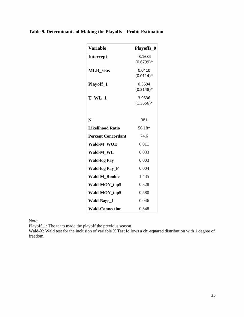
35

Table 9. Determinants of Making the Playoffs – Probit Estimation

Variable Playoffs_0

Intercept -3.1684

(0.6799)*

MLB_seas 0.0410

(0.0114)*

Playoff_1 0.5594

(0.2148)*

T_WL_1 3.9536

(1.3656)*

N 381

Likelihood Ratio 56.18*

Percent Concordant 74.6

Wald-M_WOE 0.011

Wald-M_WL 0.033

Wald-log Pay 0.003

Wald-log Pay_P 0.004

Wald-M_Rookie 1.435

Wald-MOY_top5 0.528

Wald-MOY_top5 0.580

Wald-Bage_1 0.046

Wald-Connection 0.548

Note:

Playoff_1: The team made the playoff the previous season.

Wald-X: Wald test for the inclusion of variable X Test follows a chi-squared distribution with 1 degree of

freedom.

36

Table 10. Determinants of Attendance

Variable Log

Attendance

Change in

Attendance

Intercept 1.18956 (2.91659)

5.44154

(3.58776)

NL 0.03652 (0.01932)

0.04193 (0.02385)

MLB_seas 0.00359 (0.00148)*

0.00479

(0.00183)*

l_Attend_1 0.75528 (0.03173)*

-0.31367 (0.03920)*

Change in Payroll 0.19679 (0.03654)*

0.21185 (0.04515)*

Dat_1 -0.07070 (0.04922)

-0.07516 (0.06082)

RS_1 0.000360 (0.000120)*

0.000305 (0.000148)*

Playoff_1 0.07754 (0.02586)*

0.07027

(0.03173)*

Time trend 0.00102 (0.00146)

-0.000576 (0.00180)

N 363 363

R-Square 0.7230 0.2376

White 50.30 44.43

LM-New_Hire 0.324 0.325

LM-M_WOE 0.852 0.428

LM-M_WL 0.226 0.256

LM-log Pay 0.003 0.003

LM-M_Rookie 0.792 0.217

LM-MOY & MOY_top5 1.2206 0.432

LM-Bage_1 & Page_1 1.185 0.718

LM-Log Payroll 1.620 2.094

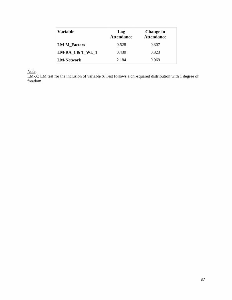
37

Variable Log

Attendance

Change in

Attendance

LM-M_Factors 0.528 0.307

LM-RA_1 & T_WL_1 0.430 0.323

LM-Network 2.184 0.969

Note:

LM-X: LM test for the inclusion of variable X Test follows a chi-squared distribution with 1 degree of

freedom.

38

Table 11. Distribution of Variables per MLB Experience

Rookie < 5 years 5-9 years 9+ years

SALARIES

Average (Standard deviation) 0.507

(0.218) 0.644

(0.448) 1.291

(0.925) 2.205

(1.373)

Sample Size (N) 41 102 58 56

MANAGER VARIABLES

Managed in Minors (% of total) 47 (62%) 139 (66%) 70 (74%) 60 (75%)

Voted in MOY top 5, at least once

(%) -

70 (33%)

90 (94%)

81 (100%)

Voted MOY, at least once (%) - 18 (9%) 36 (38%) 64 (79%)

Made Playoffs (at least once) (%) - 38 (18%) 63 (65%) 77 (95%)

MLB Winning Percentage (SD) - .491 (0.06) .505 (0.03) .517 (0.03)

Minors Winning Percentage (SD) .515 (0.04) .513 (0.04) .515 (0.03) .542 (0.03)

Minors Experience (SD) 4.042 (4.67) 4.212 (4.59) 4.438 (4.56) 3.691 (3.72)

Manager’s WOE (SD) -

0.036 (6.61) 0.402

(12.06) 10.24

(12.45)

Manager’s WOE per season (SD) -

0.072

(3.35)

-0.015

(1.86) 0.607

(0.79)

TEAM VARIABLES

Attendance, in millions (SD) 2.001

(0.83)

2.142

(0.858)

2.170

(0.943) 2.519

(0.869)

Payroll, in millions (SD) 57.30

(31.48)

58.21

(36.54)

65.69

(40.81)

76.79

(38.21)

Batting Age at t-1 (SD) 27.01 (6.95) 28.00 (4.55) 28.59 (3.24) 28.77 (3.51)

Pitching Age at t-1 (SD) 26.71 (6.91) 27.78 (4.54) 28.30 (3.20) 28.54 (3.51)

Winning Percentage at t-1 (SD) 0.480 (0.07) 0.493 (0.07) 0.494 (0.07) 0.517 (0.07)

Runs Differential at t-1 (SD) -36.17

(93.86)

-18.23

(94.98)

2.86

(101.54)

6.79

(101.01)

Made Playoffs t-1 (SD) 7 (8%) 34 (16%) 26 (29%) 24 (30%)

Value at t-1, in millions (SD) 277.88

(187.21)

284.81

(228.48)

311.17

(265.81)

349.06

(193.40)

Notes:

(%): Percent of total in category in parenthesis

(SD): Standard deviation in parenthesis

Runs Differential: Runs Scored – Runs Against

Bold: Significantly different from previous category (column).

39

Appendix: Definition of variables

Duration: Duration of manager’s contract (in years). Time t-1 variable.

Pay_year: Annual salary of MLB manager. Time t-1 variable.

Interim: Dummy variable (1 if manager was previously named interim manager). Time t-1 variable.

Fired: Dummy variable (1 if manager was fired before the end of contract). Time t-1 variable.

Seasons: Number of seasons fulfilled during contract. Time t-1 variable.

Extension: Dummy variable (1 if contract signed is an extension). Time t-1 variable.

Option: Dummy variable (1 if contract has an option provision for extra years). Time t-1 variable.

Connection: Dummy variable (1 if manager has a previous connection to a team’s GM). Time t-1

variable.

Promoted: Dummy variable (1 if manager was promoted within the organization). Time t-1 variable.

Min_coach: Dummy variable (1 if manager was a minor league coach). Time t-1 variable.

Rookie: Dummy variable (1 if manager has never coached before in MLB). Time t-1 variable.

New_Hire: Dummy variable (1 if manager is a new hire). Time t-1 variable.

NL: Dummy variable (1 if team managed is in the National League). Time t-1 variable.

MLBWL_0: Manager’s lifetime winning percentage in MLB at time of signing contract. Time t-1

variable.

MLBWL_1: Manager’s previous season winning percentage in MLB at time of signing contract. Time t-1

variable.

Winseason: Number of manager’s winning seasons in MLB. Time t-1 variable.

Av_finish: Average divisional finish of MLB teams previously managed by manager. Time t-1 variable.

MOY: Number of MOY awards. Time t-1 variable.

MOY_top5: Number of times a manager finished in the top 5 of the MOY vote. Time t-1 variable.

Award: Dummy variable if manager voted MOY at least once. Time t-1 variable.

Award_top5: Dummy variable if manager finished in the top 5 of MOY voteat least once. Time t-1

variable.

MLB_seas: Number of MLB seasons as an MLB manager. Time t-1 variable.

M_WOE: A manager’s Wins over Expected. Horwitz’s (1994) proposed performance measure. Time t-1

variable.

M_Age: Manager’s age at time of hiring. Time t-1 variable.

40

Min_Rec: Manager’s winning percentage in the minor league (if managed in the minors). Time t-1

variable.

Min_sea: Number of minor league seasons managed. Time t-1 variable.

Payroll_0: Team’s payroll at start current or just-completed season (t) a contract is signed (time t), known

at t-1. Time t-1 variable.

Payroll_1: Team’s payroll at start of the previous season (t-1) a contract is signed. Time t-1 variable.

Dpay: Change in payroll at t, known at t-1. Time t-1 variable.

Attend_0: Team’s attendance in t. Time t variable.

Attend_1: Team’s attendance in t-1. Time t-1 variable.

Attend_2: Team’s attendance in t-2. Time t-1 variable.

Dat_0: Change in attendance from t-1 to t.

Dat_1: Change in attendance at time t-1

T_WL_0: Team’s win-loss percentage record at time t.

T_WOE_0: Team’s WOE record at time t.

Finish: : Team’s divisional finish at time t.

Rel_Fin_0: Relative finish to worst team in division (lower is better) at time t.

Playoffs: Dummy variable (1 if team made the playoff at the end of seasons), time t variable.

RS_0: Team’s runs scored at end of season, time t variable.

RA_0: Team’s runs against at end of season, time t variable.

Bage_0: Team’s batting age at the end of the season time t variable.

Page_0: Team’s pitching age at the end of the season time t variable.

T_WL_1: Team’s win-loss percentage record at time t-1. Time t-1 variable.

T_WOE_1: Team’s WOE record at time t-1. Time t-1 variable.

Rel_Fin_1: Relative finish to worst team in division (lower is better) at time t-1. Time t-1 variable.

Playoffs_1: Dummy variable (1 if team made the playoff at the end of previous seasons). Time t-1

variable.

RS_1: Team’s runs scored at end of previous season. Time t-1 variable.

RA_1: Team’s runs against at end of previous season. Time t-1 variable.

Bage_1: Team’s batting age at the end of the previous season. Time t-1 variable.

Page_1: Team’s pitching age at the end of the previous season. Time t-1 variable.

41

T_WL+1: Team’s win-loss percentage record at time t+1.

T_WOE+1: Team’s WOE record at time t+1.

Rel_Fin+1: Relative finish to worst team in division (lower is better) at time t+1.

Playoffs+1: Dummy variable (1 if team made the playoff at the end of next seasons).

RS+1: Team’s runs scored at end of season, time t+1 variable.

RA+1: Team’s runs against at end of season, time t+1 variable.

Bage+1: Team’s batting age at the end of the season time t+1 variable.

Page+1: Team’s pitching age at the end of the season time t+1 variable.

Revenue_0: Team’s revenue at time t, as calculated by Forbes. Time t variable.

OpInc_0: Team’s operating income at time t, as calculated by Forbes. Time t variable.

Value_0: Team’s value at time t, as calculated by Forbes. Time t variable.

D_Value_0: Change in Team’s revenue at time t, as calculated by Forbes. Time t variable.

Val_1: Team’s value at time t-1, as calculated by Forbes. Time t-1 variable.

CarPlayApp: Manager’s career playoffs appearances. Time t-1 variable.

CarPen: Manager’s career pennant’s won. Time t-1 variable.