the value of bayesian statistics for assessing comparability
TRANSCRIPT
The value of Bayesian statistics for assessing comparability
Timothy Mutsvari (Arlenda)
on behalf of EFSPI Working Group

• Bayesian Methods: General Principles • Direct Probability Statements • Posterior Predictive Distribution
• Biosimilarity Model formulation
• Sample Size Justification
• Multiplicity • Multiple CQAs
• Assurance (not Power)
Agenda

Bayesian Methods: General Principles
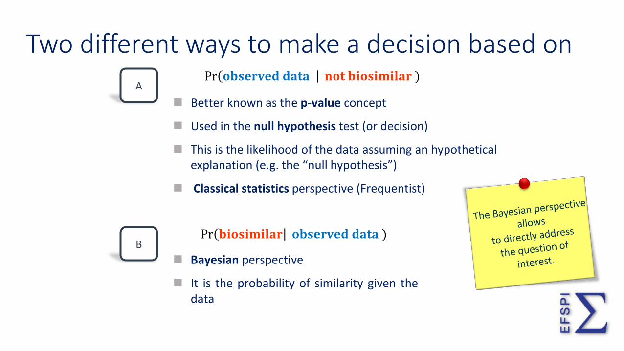
Two different ways to make a decision based on
A Pr 𝐨𝐛𝐬𝐞𝐫𝐯𝐞𝐝 𝐝𝐚𝐭𝐚 𝐧𝐨𝐭 𝐛𝐢𝐨𝐬𝐢𝐦𝐢𝐥𝐚𝐫 )
Better known as the p-value concept
Used in the null hypothesis test (or decision)
This is the likelihood of the data assuming an hypothetical explanation (e.g. the “null hypothesis”)
Classical statistics perspective (Frequentist)
B Pr 𝐛𝐢𝐨𝐬𝐢𝐦𝐢𝐥𝐚𝐫 𝐨𝐛𝐬𝐞𝐫𝐯𝐞𝐝 𝐝𝐚𝐭𝐚 )
Bayesian perspective
It is the probability of similarity given the data
3 / 18

• After having observed the data of the study, the prior distribution of the treatment effect is updated to obtain the posterior distribution
• Instead of having a point estimate (+/- standard deviation), we have a complete distribution for any parameter of interest
Bayesian Principle
P(treatment effect > 5.5)= P(success)
0 2 4 6 8 10
0.0
0.1
0.2
0.3
0.4
0.5
PRIOR distribution STUDY data POSTERIOR distribution
+
0 2 4 6 8 10
0.0
0.2
0.4
0.6
0.8
1.0
1.2

• Given the model and the posterior distribution of its parameters, what are the plausible values for a future observation 𝑦 ?
• This can be answered by computing the plausibility of the possible values of 𝑦 conditionally on the available information:
𝑝 𝑦 𝑑𝑎𝑡𝑎 = 𝑝 𝑦 𝜃 𝑝 𝜃 𝑑𝑎𝑡𝑎 𝑑𝜃
• The factors in the integrant are
- 𝑝 𝑦 𝜃 : it is given by the model for given values of the parameters
- 𝑝(𝜃|𝑑𝑎𝑡𝑎) : it is the posterior distribution of the model parameter
Posterior Predictive Distribution

Posterior Predictive Distribution - Illustration 3rd , repeat this operation a large number of time to obtain the predictive distribution
1st , draw a mean and a variance from:
Posterior of mean µi
Posterior of Variance σ²i given mean drawn
2nd , draw an observation from the resulting distribution Y~ Normal(µi, σ²i )
X X X X

Difference: Simulations vs Predictions Monte Carlo Simulations
the “new observations” are drawn from distribution “centered” on estimated location and dispersion parameters (treated as “true values”).
Bayesian Predictions
the uncertainty of parameter estimates (location and dispersion) is taken into account before drawing “new observations” from relevant distribution
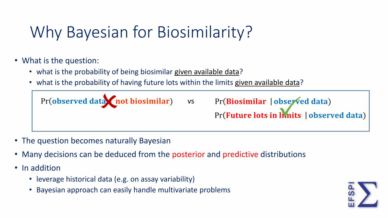
• What is the question: • what is the probability of being biosimilar given available data?
• what is the probability of having future lots within the limits given available data?
• The question becomes naturally Bayesian
• Many decisions can be deduced from the posterior and predictive distributions
• In addition • leverage historical data (e.g. on assay variability)
• Bayesian approach can easily handle multivariate problems
Why Bayesian for Biosimilarity?
Pr 𝐅𝐮𝐭𝐮𝐫𝐞 𝐥𝐨𝐭𝐬 𝐢𝐧 𝐥𝐢𝐦𝐢𝐭𝐬 𝐨𝐛𝐬𝐞𝐫𝐯𝐞𝐝 𝐝𝐚𝐭𝐚)
vs Pr 𝐨𝐛𝐬𝐞𝐫𝐯𝐞𝐝 𝐝𝐚𝐭𝐚 𝐧𝐨𝐭 𝐛𝐢𝐨𝐬𝐢𝐦𝐢𝐥𝐚𝐫)
Pr 𝐁𝐢𝐨𝐬𝐢𝐦𝐢𝐥𝐚𝐫 𝐨𝐛𝐬𝐞𝐫𝐯𝐞𝐝 𝐝𝐚𝐭𝐚)

Biosimilar Model formulation

Biosimilarity Model - Univariate Case 𝐶𝑄𝐴𝑇𝑒𝑠𝑡 ~ 𝑁 𝜇𝑇𝑒𝑠𝑡, 𝜎𝑇𝑒𝑠𝑡
2 Model for Biosimilar
𝐶𝑄𝐴𝑅𝑒𝑓 ~ 𝑁 𝜇𝑅𝑒𝑓 , 𝜎𝑟𝑒𝑓2 Model for Ref
𝜎𝑇𝑒𝑠𝑡2 = 𝛼0 ∗ 𝜎𝑟𝑒𝑓
2 Test will not extremely different from Ref
𝛼0 ~ Uniform (𝑎, 𝑏), for well chosen 𝑎 & 𝑏, e.g. 1/10 to 10
• From this model: • directly derive the PI/TI from predictive distributions
• easily extendable to multivariate model
• power computations are straight forward from predictive distributions

Model performance (compare to true pars)
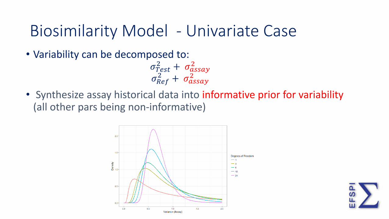
Biosimilarity Model - Univariate Case • Variability can be decomposed to:
𝜎𝑇𝑒𝑠𝑡2 + 𝜎𝑎𝑠𝑠𝑎𝑦
2 𝜎𝑅𝑒𝑓2 + 𝜎𝑎𝑠𝑠𝑎𝑦
2
• Synthesize assay historical data into informative prior for variability (all other pars being non-informative)

Bayesian PI/TI – Illustration (1)
Likelihood
(non-informative Prior on all parameters)
Predictive Distribution Tolerance Intervals (e.g.
Wolfinger)
Ref
Predictive Distributions

Bayesian PI/TI – Illustration (2)
Likelihood
Predictive Distribution Prediction Interval Predictive Distribution
Tolerance Intervals (e.g. Wolfinger)
Ref Test
Predictive Distributions (non-informative Prior on all parameters)

Bayesian PI/TI – Illustration (3)
Likelihood
Prior (informative on validated
assay variance)
Predictive Distribution Prediction Interval Predictive Distribution
Tolerance Intervals (e.g. Wolfinger)
Ref Test
Predictive Distributions

Sample Size Calculation

• Sample Test data from the predictive • How many new batches given past results to be within specs?
Sample size for Biosimilarity Evaluation

Multiplicity Extension of the univariate case

Bayesian - Multivariate CQA Model • Let
• 𝑿 be 𝑛 × 𝑘 matrix of observations for test.
• 𝒀 be 𝑚 × 𝑘 matrix of observations for ref.
𝑿
𝒀 ~ 𝑴𝑽𝑵
𝝁𝑻
𝝁𝑹,
𝜮𝑻 𝜮𝑹𝑻
𝜮𝑹𝑻 𝜮𝑹
• Any test FDA Tier1, FDA Tier2 or PI/TI can be easily computed
• Pr [𝐓𝐞𝐬𝐭 − 𝐑𝐞𝐟]|𝐃𝐚𝐭𝐚 ~ 𝑴𝑽𝑵 𝝁𝑻 − 𝝁𝑹 , [𝜮𝑻 +𝜮𝑹 − 𝟐 ∗ 𝜮𝑹𝑻]

Multivariate CQA Model • Use Ref. predictive to compute the limits of k CQAs
• Compare the Test data from k CQAs to the limits
• To get the joint test: • Calculate the joint acceptance probability

Assurance (not Power)

• Unconditional probability of significance given prior - O’Hagan et al. (2005)
• Expectation of the power averaged over the prior distribution • ‘True Probability of Success’ of a trial
• In Frequentist power is based on a particular value of the effect • A very ‘strong’ prior
Assurance (Bayesian Power)

• In order to reflect the uncertainty, a large number of effect sizes, i.e. (𝜇1−𝜇2)/𝜎pooled, are generated using the prior distributions.
• A power curve is obtained for each
effect size
• the expected (weighted by prior beliefs) power curve is calculated
Power vs assurance independent samples t-test (H0: 𝜇1 = 𝜇2 vs H1: 𝜇1 ≠ 𝜇2)
bayesian approach (assurance)
power assurance

• Using Bayesian approach: • I can directly derive probabilities of interest
• Uncertainties are well propagated
• Bayesian predictive distribution answers the very objective • probability of biosimilar given data
• future lots to remain within specs
• leverage historical data save costs
• Informative priors can be justified and recommended
• Correlated CQAs • Easily compute joint acceptance probability
Conclusions

When SIMILAR is not the SAME!