the value at risk concept in financial risk ... · pdf filethe value at risk concept in...
TRANSCRIPT
THE VALUE AT RISK CONCEPT IN THE VALUE AT RISK CONCEPT IN THE VALUE AT RISK CONCEPT IN THE VALUE AT RISK CONCEPT IN FINANCIAL RISK MANAGEMENTFINANCIAL RISK MANAGEMENTFINANCIAL RISK MANAGEMENTFINANCIAL RISK MANAGEMENT
THESISTHESISTHESISTHESIS
SUBMITTED TO THE
SWISS BANKING INSTITUTE
OF THE
UNIVERSITY OF ZÜRICH
PROF. DR. RÜDIGER FREYPROF. DR. RÜDIGER FREYPROF. DR. RÜDIGER FREYPROF. DR. RÜDIGER FREY
Subject: Monetary Economics Course: Finance Author: Theresa Ursula A. Supremo Scheuchzerstr. 27 8006 Zürich Tel. 01 362 43 51 Email: [email protected] Business Economics, 11th semester Zürich, Revised Edition as of February 2001

Executive SummaryExecutive SummaryExecutive SummaryExecutive Summary
1.1.1.1. Statement of the Problem Statement of the Problem Statement of the Problem Statement of the Problem
Arriving at a single number to depict the risk shouldered by an institution in the framework of an integrated risk management system is a great challenge. First and foremost, the risks faced by the firm should be quantifiable. Second, there should be a proper risk measurement system or analytics that is able to efficiently capture risk across different risk categories. Third, the risk measures derived should share a common unit, such that they could be aggregated. Fourth, the risk measure should behave properly in the aggregation process in the sense that there will be no incoherent consequences. For instance, if there is to be a diversification effect in the portfolio, then the risk of this portfolio should be lower than the sum of isolated risk measures derived separately for single instruments comprising it.
Currently, the quantification of market risk proceeds mainly through Value at Risk (VaR). This methodology takes the potential loss facing an instrument, portfolio or firm to be equal to the loss at a particular point of a profit and loss distribution. This is established by a predetermined confidence level and conditioned by the chosen holding period. In practice, the VaR is relatively easy to compute and communicate. However, not all VaR figures calculated using the different approaches for particular portfolios are coherent. That is, there are cases where the sum of the VaRs of individual instruments is smaller than the VaR of a portfolio consisting of these two instruments. If such holds, there will be an advantage to keep instruments, accounts, subsidiaries, and firms apart so as to keep the risk figure at a minimum. Capital adequacy or margin requirements of a portfolio can be kept low via separation of the held instruments.
But VaR is not totally incoherent. For this reason, it still retains its worth as a risk measure. Nevertheless, other methodologies have been raised as alternatives. This study will look into VaR, alternative risk measures and the concept of coherency.
2.2.2.2. Procedure of the InvestigationProcedure of the InvestigationProcedure of the InvestigationProcedure of the Investigation
Axioms that have to be satisfied by risk measures in order for them to be coherent have been raised by Artzner, Delbaen, Eber and Heath (1997, 1998). These are translation invariance, subadditivity, positive homogeneity, and monotonicity. Whether the different VaR methodologies are coherent will be investigated upon. These include the parametric VaR, historical simulation and Monte Carlo simulation methods.
Executive Summary 2
The following are the axioms of coherency against which VaR will be examined:
(1) ρ(X+ N • R) = ρ(X) N. Translation invariance specifies that the addition of a risk-free investment into a portfolio will simply reduce the risk measure by as much as the value of the investment.
(2) ρ(X + Y) < ρ(X) + ρ(Y). Subadditivity states that the risk of a portfolio consisting of two instruments should be lower than or equal to the sum of the individual risks of the instruments.
(3) ρ(λ • X) = λ • ρ(X). Positive homogeneity upholds the risk of one and the same instrument to be void of any incremental risk, once the position is scaled. Increasing the size of the instrument by λ increases its risk by λ. Liquidity is hereby assumed.
(4) ρ(X) ≥ ρ(Y), if X < Y. Monotonicity proposes a ranking specification of risk measures of differing instruments. The smaller the portfolio returns, the greater is its risk.
3.3.3.3. ResultsResultsResultsResults
Parametric VaR or the variance-covariance approach builds on the mean and variance of a profit and loss distribution to come up with the potential loss of an instrument or portfolio, given a holding period and confidence level. The assumption made is that risk factor movements follow a normal distribution. This determines the consequently normally distributed profit and loss distribution. Knowing the portfolio mean and variance, one could easily calculate the VaR of a particular confidence level. The VaR is the difference between the mean and the value at the specified quantile of the distribution. One actually arrives at this on the basis of the variances of the risk factors. The weighted variances are added together, while allowing for correlations. The total volatility is then multiplied with the corresponding quantile factor. Analyzed as against the axioms of coherency, parametric VaR qualifies as a coherent risk measure. This holds for a distribution with a confidence level above 50% and a joint multivariate normal distribution of risk factors. The accuracy of the risk measure can however only be certified under the delta-normal approach. This approach assumes a linear relationship of the risk factors to the value of the portfolio. The existence of non-linear relationships in the portfolio, e.g. options, cannot be efficiently captured. Furthermore, satisfactory results cannot be reached with the use of the specialized delta-gamma approach.
In contrast, the VaR derived from historical simulation does not always satisfy the most crucial subadditivity axiom. The sum of the VaR of a given portfolio X and portfolio Y is, in some cases, smaller than the VaR of a portfolio with X and Y together. Historical simulation arrives at the VaR by taking historical data on the risk factors and inputting them into the valuation formula of the given instrument or portfolio. These are then subtracted from the current value. The VaR is the value at
Executive Summary 3
the specified quantile of the number of days or data chosen. Why this methodology sometimes comes up with superadditive values lies in the fact that the percentile VaR calculated for a portfolio combination of individual instruments is largely dependent on the valuation function of the portfolio and the factors inputted, whose correlations are not taken into consideration. The values that are entered to construct the profit and loss distribution of the chosen period fall into play arbitrarily.
The same holds for the VaR results of Monte Carlo simulation. Subadditivity is not at all times respected. Under this methodology, the values of risk factors follow a process specified by a random generator. Similar to historical simulation, the VaR is the value at the specified quantile of the resulting randomly generated profit and loss figures. The VaR is thus made dependent on the inputted risk factors, whose correlations need not be considered by such a random generation of the risk factor values. The portfolio VaR need not be the same as the sum of the individual VaRs of the instruments. It may even exceed it, depending on the portfolio components.
As an alternative to VaR, the maximum loss methodology has been upheld by Studer (1997) as a coherent risk measure that moreover captures the non-linear behavior of portfolios efficiently. Under maximum loss, probability information is made use of to arrive at the likely loss that the portfolio will face, given a particular threshold of risk factor values or a trust region. A whole distribution need not be set up. The minimum of the values of the profit and loss function derived on the basis of the selected risk factor values is the maximum loss. Correlations between the risk factors are carried over by the risk factor processes assumed.
Another coherent risk measure can be derived from the expected shortfall methodology. The expected shortfall is the average of the losses of an instrument that is beyond a given benchmark or limit. It has a quite simple methodology and provides information on the extent of loss beyond VaR or any given benchmark value.
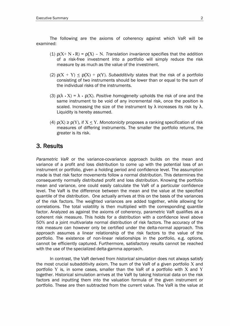
The following is a tabular summary of the coherency of the risk measures considered:
Risk Measures
Translation Invariance
ρ(X + R • N) = ρ(X) N
Positive Homogeneity
ρ(λ • X) = λ • ρ(X)
Subadditivity
ρ(X + Y) < ρ(X) + ρ(Y)
Monotonicity
If X > Y, then ρ(X) < ρ(Y)
Parametric VaR
For portfolios with linearly related risk factors with a joint normal distribution and a confidence level above 50%
Historical Simulation
Not always
Monte Carlo Simulation
Not always
Maximum Loss
Expected Shortfall
Executive Summary 4
VaR is disadvantaged by its occasional non-adherence to the axiom of subadditivity. Moreover, a look into the computational framework of the different methodologies indicate how some methodologies do not efficiently capture the true VaR. Parametric VaR, as said, buckles down when the portfolio involves non-linear components. Fat tails, which occur in reality, are also not efficiently captured. Monte Carlo simulation is in this regard better. Variations in time and extreme scenarios are also captured. The modeling used in Monte Carlo should however take pains to capture reality as most probably done by a historical simulation. In line with accuracy, other dependence measures other than correlation should perhaps be looked into in order to capture well the intricacies of non-linear relationships, which are not considered by the distributional assumptions of correlation measurement.
4.4.4.4. General EvaluationGeneral EvaluationGeneral EvaluationGeneral Evaluation
In spite of its drawbacks, VaR however continues to dominate in the risk measurement practice. Current research on credit risk measurement is also heading towards the direction of VaR-based measurement. That is, credit-at-risk akin to value-at-risk is sought to be measured. Making credit risk measurement compatible with VaR will facilitate in the near future the integration of market and credit risk factors into a single risk measure derived from the same VaR-based methodology.
What are the prospects for the extensive use of expected shortfall and maximum loss? Considering the wide acceptance of VaR, a sharp turn towards these alternative methods is not to be expected. These may however not be the case in the long run. Adhering to coherency without hitches, expected shortfall and maximum loss measurement could be the upcoming tools of integrated risk management.
Subadditivity is indeed a relevant consideration. Its violation leads to dumb consequences. It cannot be that a trader would have an advantage of separating two instruments from each other, because he or she will be required lesser capital for the maintenance of these instruments in isolation as compared with holding them in a portfolio. Knowing that VaR measurement has occasional troubles with subadditivity should not simply be laid aside. The information that VaR provides is however of worth, such that VaR measurement remains feasible. For as long as subadditivity is respected in capital requirement measurement, VaR could still come up with reliable information.
But adherence to the axioms of coherency need not be the criterion in choosing the best risk measurement methodology. Much as the axioms are helpful in the determination whether particular risk measures are sound for whatever purpose that they may serve, e.g., for capital or margin requirements, the axioms of coherency should not be the ultimate basis for choosing an appropriate risk measurement methodology. If we use risk measures for investment choice, then the axioms are not sufficient, because what they emphasize is the behavior of the risk measures. No focus is given on the returns.

Executive Summary 5
Possible grounds for choosing a risk measurement methodology are its usefulness in the analyses required by the firms financial activities. Others could revolve around economic considerations and the type of additional information that the methodology yields. The simplicity of its application is also a plus factor, although not the most essential. The following table summarizes the properties of the different risk measurement methodologies against the four enumerated criteria:
VaR Maximum Loss Expected Shortfall
Coherency Subadditivity violated at times
Coherent Coherent
Information provided
The potential loss specified at a chosen quantile of a distribution
The minimum of the profit and loss function of a dense trust region of risk factor values; it captures non-linear behavior efficiently
The mean of the expected losses beyond a benchmark value
Economic considerations
Simulation infrastructure requires much resources
The calculation requires much resources
Relatively fewer data requirements
Simplicity Simple Complex Simple
In this regard, expected shortfall gains ground against the other risk measurement methodologies, as its methodology is coherent, simple and economical. There is also additional information on the extent of loss beyond a certain established tolerance level.
But whatever risk measurement methodology be in prominent use in the future, what is important is that the risk measure indeed captures what is desired to be captured by a particular analysis, may it be for total enterprise-wide risk management or investment choice analysis decisions. Coherency is necessary. But so is axiomatic investigation validity.
Table of ContentsTable of ContentsTable of ContentsTable of Contents
List of FiguresList of FiguresList of FiguresList of Figures................................................................................................................................................................................................................................................................................................................................................ iiiiiiii List of TablesList of TablesList of TablesList of Tables .................................................................................................................................................................................................................................................................................................................................................... iiiiiiii List of Abbreviations and SymbolsList of Abbreviations and SymbolsList of Abbreviations and SymbolsList of Abbreviations and Symbols ........................................................................................................................................................................................................ iiiiiiiiiiii Chapter 1Chapter 1Chapter 1Chapter 1 INTRODUCTIONINTRODUCTIONINTRODUCTIONINTRODUCTION....................................................................................................................................................................................................................................................1111
1.1 Historical Background............................................................................................. 1
1.2 Regulatory Requirements....................................................................................... 2
1.3 Risk and its Different Types.................................................................................... 3
Chapter 2Chapter 2Chapter 2Chapter 2 THE VALUE AT RISK CONCEPTTHE VALUE AT RISK CONCEPTTHE VALUE AT RISK CONCEPTTHE VALUE AT RISK CONCEPT ....................................................................................................................................................5555
2.1 What is Value at Risk? ............................................................................................ 5
2.2 Calculating Value at Risk........................................................................................ 7
2.2.1 Parametric VaR ............................................................................................... 7
2.2.2 Historical Simulation.....................................................................................12
2.2.3 Monte Carlo Simulation................................................................................15
2.3 Criticisms on VaR ..................................................................................................16
2.3.1 General Evaluation .......................................................................................16
2.3.2 Summative Evaluation from a Computational Perspective .......................18
Chapter 3Chapter 3Chapter 3Chapter 3 Value at Risk and CoherencyValue at Risk and CoherencyValue at Risk and CoherencyValue at Risk and Coherency ................................................................................................................................................ 20202020
3.1 Coherency..............................................................................................................20
3.1.1 Translation Invariance [ρ(X+ N • R) = ρ(X) N] .........................................21
3.1.2 Subadditivity [ρ(X + Y) < ρ(X) + ρ(Y)] ........................................................21
3.1.3 Positive Homogeneity [ρ(λ • X) = λ • ρ(X)] ...................................................21
3.1.4 Monotonicity [ρ(X) ≥ ρ(Y), if X < Y] ...............................................................22
3.2 The Coherency of VaR...........................................................................................22
3.2.1 The Coherency of Parametric VaR (Delta-Normal) .....................................23
3.2.2 The Coherency of Historical Simulation ......................................................24
3.2.3 The Coherency of Monte Carlo Simulation..................................................27
3.3 Alternatives to VaR................................................................................................28

ii
3.3.1 Maximum Loss ..............................................................................................28
3.3.2 Expected Shortfall.........................................................................................30
Chapter 4Chapter 4Chapter 4Chapter 4 CONCLUSIONCONCLUSIONCONCLUSIONCONCLUSION .................................................................................................................................................................................................................................................... 35353535
ReferencesReferencesReferencesReferences ............................................................................................................................................................................................................................................................................................................................................ 39393939
LiLiLiList of Figuresst of Figuresst of Figuresst of Figures
Figure 1: An overview of the value-at-risk concept...................................................... 5
Figure 2: Value at risk methodologies.......................................................................... 6
Figure 3: Parametric VaR methods .............................................................................. 7
Figure 4: Expected Shortfall.......................................................................................... 31
List of TablesList of TablesList of TablesList of Tables
Table 1: Hypothetical data used for the historical simulation VaR............................ 15
Table 2: Summary of the features of VaR.................................................................... 17
Table 3: Problematic factors related to mathematical considerations ..................... 18
Table 4:Subadditivity of the parametric VaR of elliptical distributions...................... 23
Table 5: Positive homogeneity of parametric VaR ...................................................... 24
Table 6: Subadditivity of the VaR per historical simulation........................................ 25
Table 7: Violation of subadditivity of percentile VaR................................................... 25
Table 8: Positive homogeneity of VaR per historical simulation ................................ 26
Table 9: Data on portfolios X and Y .............................................................................. 33
Table 10: Expected shortfall of the portfolio of X and Y together .............................. 33
Table 11: Subadditivity of expected shortfall .............................................................. 33
Table 12: Comparison of VaR, maximum loss and expected shortfall...................... 37
iii
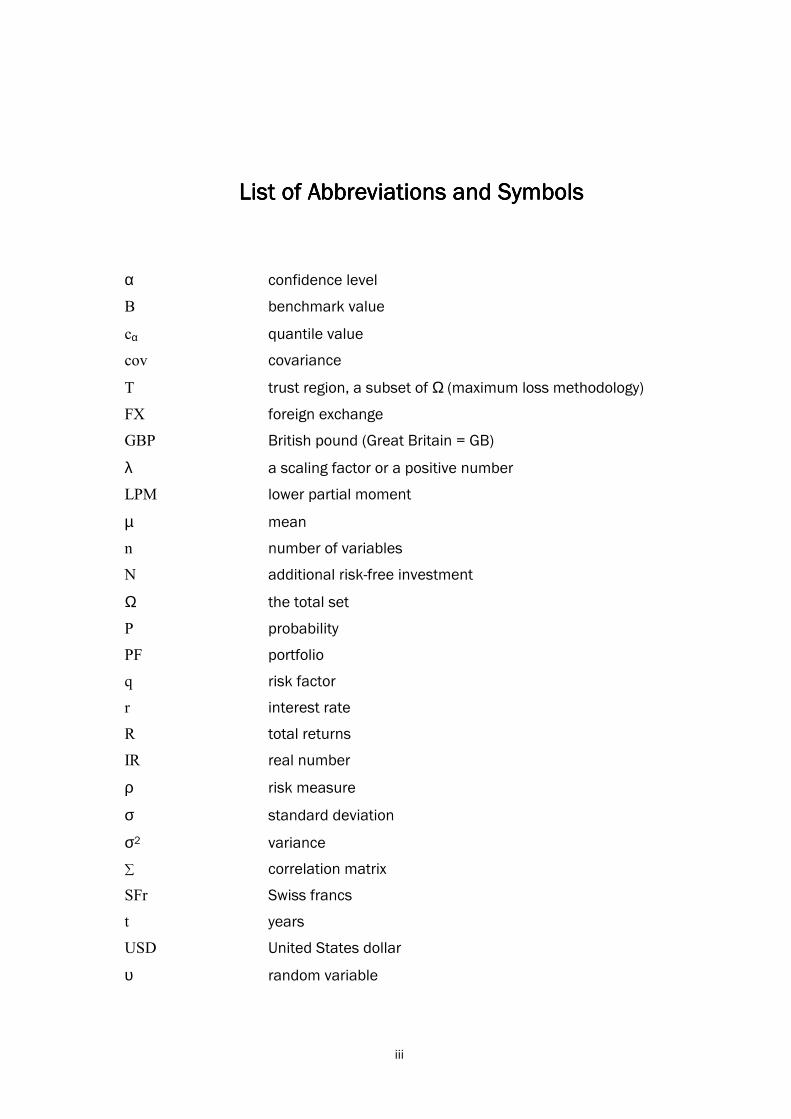
List of Abbreviations and SymbolsList of Abbreviations and SymbolsList of Abbreviations and SymbolsList of Abbreviations and Symbols
α confidence level
B benchmark value
cα quantile value
cov covariance
T trust region, a subset of Ω (maximum loss methodology)
FX foreign exchange
GBP British pound (Great Britain = GB)
λ a scaling factor or a positive number
LPM lower partial moment
µ mean
n number of variables
N additional risk-free investment
Ω the total set
P probability
PF portfolio
q risk factor
r interest rate
R total returns
IR real number
ρ risk measure
σ standard deviation
σ2 variance
correlation matrix
SFr Swiss francs
t years
USD United States dollar
υ random variable

iv
υ(ω) a profit and loss function or a random value function
V(X) value of a security X
VaR Value at Risk
w weight factor
[w] sensitivity vector (VaR)
[w]t transposed sensitivity vector (VaR)
ω scenario, random value
X a security or returns of a security X
Y a security or returns of a security Y

Chapter 1Chapter 1Chapter 1Chapter 1 INTRODUCTIONINTRODUCTIONINTRODUCTIONINTRODUCTION
1.11.11.11.1 Historical BackgroundHistorical BackgroundHistorical BackgroundHistorical Background
Risk management has gained much importance over the years. Incidence of catastrophic investments that were not subjected to careful surveillance caught the attention of several financial institutions. Primary importance has then been given to the development of strategies to prevent financial mishaps, as well as to the measurement of the potential loss faced by the firm.
A look at historical developments shows us how markets have fluctuated increasingly. In other words, market variables have grown to be quite volatile. With the flexibility lent to the exchange rates of various currencies against the dollar back in the 1970s, exchange rate fluctuations and its repercussions onto other market factors became mighty powers behind international market developments. Moreover, increased international capital mobility and reduced trade barriers have paved the way for a high level of market interdependence. Effects of stock market crashes, oil price shocks and financial crises have thus crossed national and regional borders. We have witnessed this in the case of the Asian financial crisis, which has turned several stock markets haywire not only in Asia but also in Russia and in the Americas. The threat of contagion faced subsequently by industrial countries is indicative of the fact that sound fundamentals do not provide a surefire assurance against financial market turmoil.
Meanwhile, several types of financial instruments have surfaced not only as a way of insuring firms from catastrophic outcomes but also as a result of innovations fostered by developments in financial theory and technology. But the variety of products, the numerous possibilities they allowed and the strategies and ensuing rampant speculation taken on by various institutions have also contributed to market uncertainties. The renowned case of the failure of the high-risk Long Term Capital Management fund and the brouhaha it caused attest to this fact.
Risk management has thus become a must in view of the volatile and increasingly complex market. The delivery of a single number that would spell out the potential loss faced by a firm was first conceptualized and launched by J. P. Morgan in 1994. If not for previous developments in financial theory such as the Markowitz portfolio theory and Sharpes model of security risk set against a market index, the emergence of such a conceptualization would not have materialized. Quite revolutionary, J. P. Morgans so-called 4:15 reports demanded a clear-cut figure indicating succinctly the risk exposure of the firm an improvement from other
Chapter 1: Introduction
2
analyses such as duration and gap. To accomplish this, a system had to be set up in order to come up regularly with a quick estimate. Correlations taken into consideration, a single estimate would already indicate how much of a given value is at risk. This was called the Value at Risk (VaR). With its public disclosure and incorporation in regulatory risk measurement systems, the VaR technique grew in popularity.
1.21.21.21.2 Regulatory RequirementsRegulatory RequirementsRegulatory RequirementsRegulatory Requirements
The use of VaR to come up with capital adequacy level requirements was put forward by regulatory authorities. In 1996, the recommended techniques for risk measurement entailed VaR measurement.
If we take a look at the historical flow of events, we would note that the need for risk management and measurement was first officially put into paper by the Bank of International Settlement (BIS) in 1988. Sufficient capital as coverage against credit risk was required. This was equal to 8% of the total risk-weighted assets, 50% of which must be stock issues and disclosed reserves. Moreover, large risks pertaining to exposures that entail more than 10% of a banks capital was restricted.
In 1996, market risk was added into the consideration. This came about because of the aforementioned market developments primarily characterized by market volatility and increased incidence of financial debacles. Sufficient capital must be held to cover market risks as well. Two possibilities towards the encapsulation of the potential risks were laid down: a standard BIS-formulated approach and an internally adopted approach subject to quantitative and qualitative criteria. The standard methodology utilizes a building block approach for the calculation of the potential risk for every risk category. It is based on the VaR concept.
In the light of recent developments including the financial crisis of the late 1990s, a new capital adequacy framework is currently being worked upon. Intensive analyses are undertaken to find the appropriate capital charges for interest rate risks in the banking book for banks with highly risky investments.1 The proper treatment of operational risks is also under study. In general, three pillars have already been put forward: minimum capital requirements, a supervisory review process and the effective use of market discipline.
Capital requirements have always been central from the very beginning. Hence, this pillar entails the same fundamental concepts as before. VaR continues to be the primary method recommended in the estimation of risk, although the standard approach is on review. Mainly, a new risk-weighting scheme and the
1 In the 1996 amendment, only the trading book was relevant in the calculation of the interest and equity risks.

Chapter 1: Introduction
3
allowance of alternative internal ratings-based approaches are being sought. Moreover, the standardization of approaches in portfolio credit risk modeling, as well as the approaches used in measuring risks from credit derivatives and other instruments, is being looked into. The main thrust is to improve the way regulatory capital requirements reflect underlying risks. It is also sought to better address the financial innovations of the recent years. The advent of innovations has made the current regulation less effective in matching capital requirements with a banks true risk profile.
The need for the second pillar a supervisory review process has come up to ensure that a banks capital position is consistent with its overall risk profile and strategy. This has been fashioned to encourage early supervisory intervention. Supervisors will have the ability to require banks to hold capital in excess of the minimum required capital. This has not been covered by earlier frameworks as the consideration was centered on the conditions of the G-10 countries, which contributed to the drafting of the existing regulation. As for the third pillar on market discipline, the main aim is to encourage disclosure or transparency.2
1.31.31.31.3 Risk and its Different TypesRisk and its Different TypesRisk and its Different TypesRisk and its Different Types
Risk management is a policy-based measurement, regulation and control system of the risks affecting the financial activities of an institution. Insofar as a total risk figure is sought for a whole firm encompassing several types of risk we speak of integrated risk management or enterprise-wide risk management. Risk, on its part, is the uncertainty involving future developments that affect the value of an instrument. This definition does not leave out the occurrence of excessive, rarely occurring positive returns at a certain point, which could actually turn out bad at a later time. Thus, a large dispersion from the normal case whether towards negative or positive extremes means a high degree of riskiness. Risk can take on many forms or can be grouped into different categories:
Business risk is the uncertainty faced in view of the particular business activity that has been taken on. For example, European airlines face the business risk that more and more people utilize speedy trains for short routes instead of boarding a plane. The jet business might prove to be unprofitable in the long run. Financial risk, meanwhile, encompasses the uncertainty involving future developments that affect the value of asset holdings and possibly impair liquidity or solvency.
Financial risk can ensue from various sources:
2 Cf. BIS (2000a), pp. 1-2.

Chapter 1: Introduction
4
Market risk is the uncertainty or potential adversity faced by financial assets or values due to fluctuations in market factors, such as stock prices, indices, commodity prices, interest rates and exchange rates.
Credit risk is the uncertainty or potential adversity faced by capital lenders due to developments that affect their lending activities. Movements in interest rates could for example be detrimental to the value of debt. Moreover, losses can ensue from a downgrading, since debt market value recedes. Credit risk is also oftentimes referred to as default risk. As a matter of fact, several literature take credit risk to be default risk. The thin line that demarcates them is the fact that the latter refers concretely to the potential adversity resulting from the prospect that a given agreement will not be honored by a counterparty, may it be a credit or a swap agreement, whereas credit risk need not end up with an actual failure of payment. Nevertheless, default risk is the primary component of credit risk, and both types of risk are affected by the same set of factors. That is the reason behind their assumed synonymy. Moreover, insofar as the solvency of the borrower is affected by market risk, credit risk and default risk are intertwined with market risk.
Liquidity risk is the potential adversity ensuing from difficulties in dissolving, e.g., encashing, a given asset at a particular point in time. This type of risk is however difficult to quantify. A standard or universal liquidity risk measurement approach has not yet been laid down.
Similarly, the appropriate measurement of operational risk is still in question. Operational risk is the potential adversity faced as a result of system failures or manipulations. Measuring this requires both estimating the probability of an operational loss event and the potential size of the loss.3
Legal risk is the potential adversity arising from various lawfully imposed conditions: non-enforceability of a particular transaction or business activity, penalties from non-compliance of regulations including lawsuits, etc.
To perform its function well, risk management relies on the accuracy of the adopted risk measurement technique for the above-mentioned risk types. Risk measurement could however not proceed if the risk is not quantifiable. If it were quantifiable, then the risk measurement methodology or analytics used should come up with risk measures having a common unit in order to add them all up.
VaR measurement is focused on the measurement of market risk. The inclusion of credit risk into the VaR figure will have to consider closely the correlations existing between these two types of risk, albeit the VaR already has the problem of ensuring the consideration of the correlations between the different market risk factors. Insofar as the VaR comes up with an aggregate risk figure, it is a useful tool in integrated risk management.
3 Cf. BIS (2000b), p. 4.

Chapter 2Chapter 2Chapter 2Chapter 2 THE VALUE AT RISK CONCEPTTHE VALUE AT RISK CONCEPTTHE VALUE AT RISK CONCEPTTHE VALUE AT RISK CONCEPT
2.12.12.12.1 What is Value at Risk?What is Value at Risk?What is Value at Risk?What is Value at Risk?
The Value at Risk is a numerical figure signifying the potential loss of an asset or portfolio, given a certain holding period and confidence level. The holding period is the length of time that a security or portfolio is held or the specific time horizon chosen for the analysis, whereas the confidence level is a statistical property denoting in percentage form the boundary level of the values or the probability of occurrence of a particular value. For instance, a 95% confidence level denotes the quantile or percentile corresponding to 95% of the whole set of calculated values. Selecting a confidence level is thus akin to specifying a tolerance level for the change in values. Choosing the holding period and confidence level proceeds arbitrarily, although it has implications on the derived VaR.
Concretely, if we have an asset X, the value that we are at risk of losing, say, in a days time at a 95% confidence level is the difference between the mean of the assets value and the value at the 95th quantile of the probability distribution of the assets values after one day. The VaR is equal to the distance X95% and µ. We are 95% sure that the loss over one day will not exceed this amount. This is illustrated in Figure 1.
Figure 1: An overview of the value-at-risk concept
σσσσ
X95% µ
VaR
Value-at-Risk (VaR)
Value

Chapter 2: The Value at Risk Concept
6
We see here that the VaR is dependent on the left-side boundary value corresponding to the selected tolerance level. The µ and σ stand for the mean and standard deviation of the distribution, respectively.
In simple mathematics, the VaR is generally:
α−µ= X)relative(VaR , (1 )
where µ is the expected value of the asset X, and Xα is the value of X at the chosen confidence level.
The above equation results to a VaR relative to the mean. VaR may also be taken relative to 0. The VaR in this case will then be an absolute potential loss. It is equal to the negative of the value of the asset or portfolio at the selected confidence level:
α−= XX)absolute(VaR 0 , (2 )
where X0 is equal to zero.
Note that in a standard normal distribution, the mean is always equal to zero.
As already seen, a distribution is required for the VaR computation. Methods used in arriving at a distribution may vary, depending on the type of approach preferred to arrive at the VaR. These several approaches with which the VaR may be calculated may be classified in various literature differently, but some order could be established. In general, VaR methodologies can be classified into two: analytical and numerical. Figure 2 provides an overview of the VaR methodologies broken down to their approaches.
Value at Risk Methods
Analytical Numerical
Parametric VaR
Historical Simulation
Monte Carlo
Simulation
Figure 2: Value at risk methodologies
Source: Brouwer/Densing (2000)
Chapter 2: The Value at Risk Concept
7
Briefly, analytical VaR denotes an assessment of the parameters that underlie a profit and loss distribution. The approach that belongs to this type is the parametric VaR. Numerical VaR, on the other hand, is a calculation of VaR based on serial data4, as its name implies. This includes the historical simulation and Monte Carlo simulation approaches.
Parametric VaR, historical simulation and Monte Carlo simulation are normally the three approaches discussed by various literature. The following sections undertake an explanation on the risk measurement followed by these approaches.
2.22.22.22.2 Calculating Value at RiskCalculating Value at RiskCalculating Value at RiskCalculating Value at Risk
2.2.12.2.12.2.12.2.1 PaPaPaParametric VaRrametric VaRrametric VaRrametric VaR
Parametric VaR is a method that calculates the parameters underlying a profit and loss distribution, i.e., mean and standard deviation, in order to come up with the potential loss of an asset or portfolio, given a holding period and confidence level. After deriving the mean and standard deviation, statistical theory is applied to come up with a VaR estimate. This is the reason why it is referred to as parametric VaR or the variance-covariance approach. VaR is determined via parametric information.
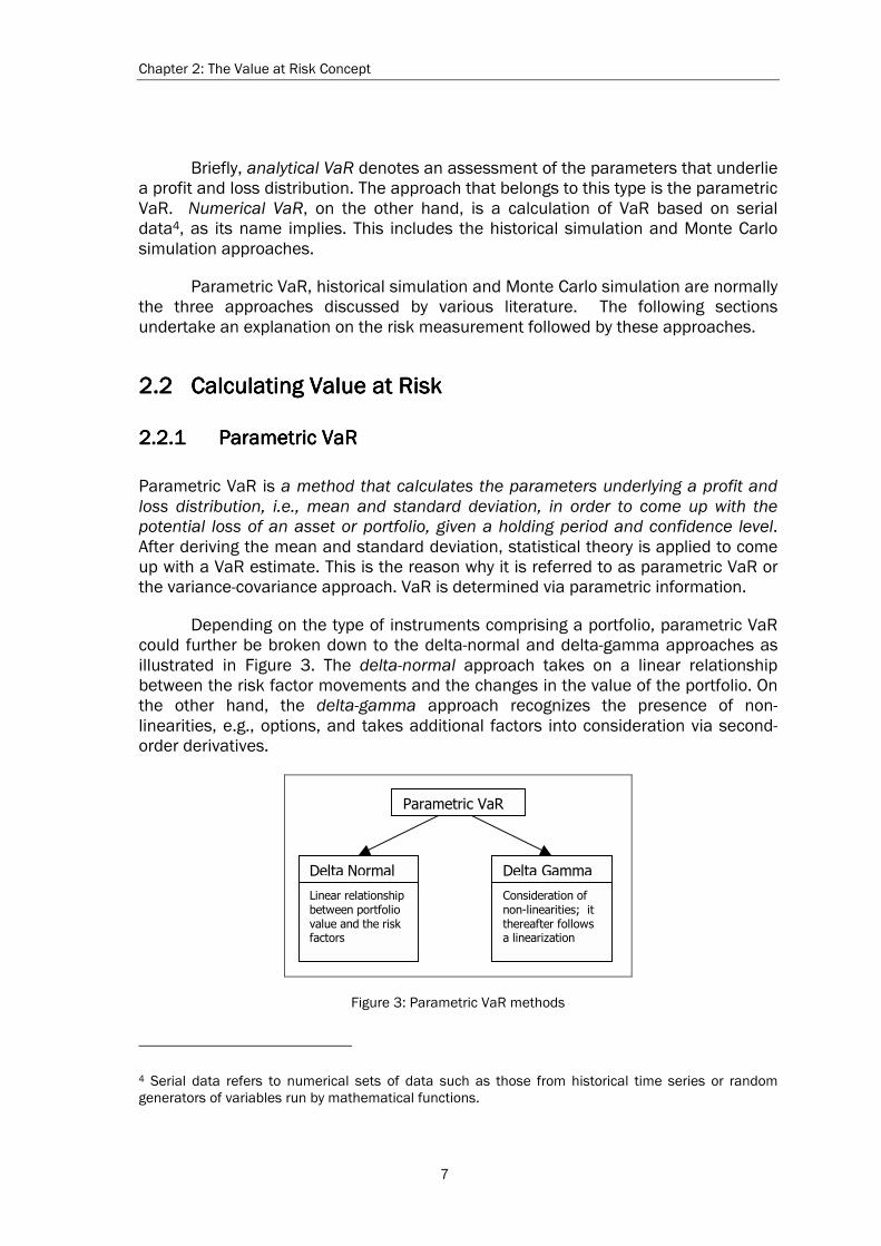
Depending on the type of instruments comprising a portfolio, parametric VaR could further be broken down to the delta-normal and delta-gamma approaches as illustrated in Figure 3. The delta-normal approach takes on a linear relationship between the risk factor movements and the changes in the value of the portfolio. On the other hand, the delta-gamma approach recognizes the presence of non-linearities, e.g., options, and takes additional factors into consideration via second-order derivatives.
Parametric VaR
Delta Normal Delta Gamma
Linear relationship between portfolio value and the risk factors
Consideration of non-linearities; it thereafter follows a linearization
Figure 3: Parametric VaR methods
4 Serial data refers to numerical sets of data such as those from historical time series or random generators of variables run by mathematical functions.
Chapter 2: The Value at Risk Concept
8
Risk factor movements determine the profit and loss distribution, and ergo, the mean and standard deviation. A set of risk factors that are known to affect the value of the asset is then required for the analysis. From the assumed movements in the risk factors, the distribution of profits and losses of the asset or portfolio can be constructed. It is further assumed that a given risk factor distribution applies for the whole length of the period covered. Moreover, as the individual risk factors accounted for in the distribution are not independent of each other, correlations are taken into account. This will be elucidated in the coming section.
2.2.1.1 Delta-Normal Method
The delta-normal method is a parametric VaR method that arrives at the VaR after building a distribution of profit and loss values based on an assumption of a linear relationship between the value of a position and the movements of underlying risk factors. A further assumption is that such risk factor movements follow a normal distribution. Consequently, the resulting distribution of values is also normal.
To illustrate the assumption of linearity, let us for example assume that two risk factors affect the value of a portfolio X. The sensitivity or delta of the portfolio value with respect to two risk factor changes is expressed as follows:
22
11
dqq
)X(Vdq
q
)X(V
dq
)X(dV
∂∂+
∂∂≈ , (3 )
where V(X) is the value of a portfolio X, whereas q1 and q2 represent the two risk factors.
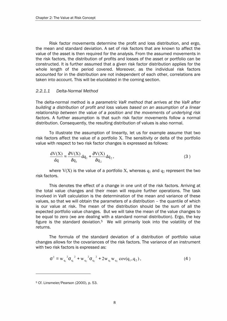
This denotes the effect of a change in one unit of the risk factors. Arriving at the total value changes and their mean will require further operations. The task involved in VaR calculation is the determination of the mean and variance of these values, so that we will obtain the parameters of a distribution the quantile of which is our value at risk. The mean of the distribution should be the sum of all the expected portfolio value changes. But we will take the mean of the value changes to be equal to zero (we are dealing with a standard normal distribution). Ergo, the key figure is the standard deviation.5 We will primarily look into the volatility of the returns.
The formula of the standard deviation of a distribution of portfolio value changes allows for the covariances of the risk factors. The variance of an instrument with two risk factors is expressed as:
)q,qcov(ww2ww 21qq2
q2
q2
q2
q2
212211+σ+σ=σ , (4 )
5 Cf. Linsmeier/Pearson (2000), p. 53.

Chapter 2: The Value at Risk Concept
9
where w1q and w
2q signify the weighting6 of the risk factor change as we are purporting here a linear relationship, and cov(q1, q2) is the covariance of the two risk factors.
The challenge is then to find out the variances of the individual risk factor changes and their correlation or covariance. The variance of the portfolio is expressed as the sum of the variances and covariances.
What if there are more than two risk factors? The variance formula will be:
+ σ=σ= ≠==
n
1i
n
ij,1jjijqiq
n
1i
2
iq2
iq2 )q,qcov(www (5 )
In matrix form, this will be:
[ ] [ ]ww t2 Σ=σ , (6 )
where Σ represents the covariance matrix, and [w] is the variance vector.
What is then the value at risk? Fundamental to the determination of the VaR is the choice of the holding period and confidence level. Given that the holding period and confidence level has been determined, the VaR may then be calculated as:
( )[ ]σα−µ=VaR , (7 )
where α is the statistically derived value corresponding to the desired quantile to be multiplied with the standard deviation (e.g., 1.65 for a 95% confidence level).
If the mean is equal to zero, the VaR could be reduced as:
)(VaR σα−= (8 )
or in matrix form:
]w[]w[VaR t Σα−= . (9 )
Given the VaRs of individual instruments, the portfolio VaR is:
[ ] [ ] [ ]VaRVaRVaR t ⋅Σ⋅−= ,7 (10 )
6 This will be the sensitivities in the portfolio, i.e., ∂V(X)/∂qi* qi. 7 Cf. Biermann (1999), p. 112. The transformation of Equation 9 to this expression is indicated therein.
Chapter 2: The Value at Risk Concept
10
which is similar to our standard deviation equation in matrix form.
This is the general idea behind parametric VaR and more specifically, the delta-normal approach. But the method through which the parameters are taken may vary. Risk mapping, for instance, is a RiskMetrics methodology that reduces the instruments within the portfolio into simple, approximating instruments, whose sensitivities are estimated. This avoids the task of computing numerous variances.
Given the assumptions, parametric VaR is relatively fast and easy to compute and not too prone to model risk. The data requirements are also considerably attainable. The number of criticisms, as summarized below, might be disconcerting, but it should be noted that this methodology has in practice provided good approximations of the VaR. The standard deviation provides far more information than mere quantiles based on values taken from history or a random generation function.8 Moreover, in terms of utility theory-based analyses, this is the only VaR approach does not violate the rational ranking of choices based on expected utility value.9 Among the criticisms are10:
- The stipulated linear relationship of the risk factors to the value of the position is only an approximation. Portfolios containing a significant number of options may not be optimally assessed.
- The size of the covariance matrix increases geometrically as the number of assets increases.
- It assumes a normal distribution of returns. This is negated by empirical evidence that suggest fat tails.
- Volatility is taken to be a function of the assumed normal distribution of risk factor returns weighted by sensitivities. Whether volatility is indeed determined by this function is uncertain. It is observable that prices are also conditioned by the conditions of the times. If prices yesterday were volatile, it will also likely be volatile tomorrow. Just as the stochastic process followed by price movements is under question in financial theory, the volatility function espoused here is an inference.
- It is greatly disadvantaged under extreme situations. It accounts for such situations as stock market crashes or exchange rate collapses poorly. This is thus related to the previous criticism.
- It conducts purely a static analysis. Changes that ensue in time and through changes in portfolio composition are not considered.
8 The other VaR calculation methods are discussed subsequently. 9 Cf. Guthoff/Pfingsten/Wolf (1998), pp. 133 and 136. 10 Cf. Jorion (2000), pp. 220-221, and Brouwer/Densing (2000), pp. 5 and 10.

Chapter 2: The Value at Risk Concept
11
To remedy the non-consideration of non-linear relationships in the portfolio, the delta-gamma method provides an alternative approach at VaR calculation.
2.2.1.2 Delta-Gamma Method
The delta-gamma method is a parametric VaR approach that recognizes non-linear relationships in an instrument or portfolio by adding additional factors into the profit/loss equation that capture non-linear behavior. This means that we do not plainly assume constant, linear relationships between the value of the portfolio and its risk factors just as in the delta-normal method. Under the delta-gamma method, the non-linear relationships are first estimated and then inputted into the linear equation as an approximation of the non-linearities.
Non-linear relationships are for example present in portfolios containing options. The value of the portfolio is thereby dependent on the underlying value of the variable upon which the contained option is dependent. These non-linearities are captured by means of a Taylor expansion. Not just the delta or the sensitivity of the portfolio of the risk factor is required; the options gamma or its second order term is calculated.
Under the delta-normal method, we already have the sensitivity of the portfolio value with respect to the option as a linearly related term. This is for instance the first term of right side of Equation 11 . The delta-gamma method then applies the Taylor expansion as shown by the succeeding terms:
...dtt
)X(Vdq
q
)X(V
2
1dq
q
)X(V
dq
)X(dV 2
2
2
+∂
∂+∂
∂+∂
∂≈ , (11 )
which, in using ∆ for the sensitivity, Γ for the second order term and Θ for the time drift, is equal to:
...dtdq2
1dq
dq
)X(dV 2 +Θ+Γ+∆≈ . (12 )
To arrive at the VaR, the standard deviation is required, just as in the delta-normal method. This is:
)dq,dqcov(2
12dq
2
1dq 222
2222
Γ∆+σ
Γ+σ∆=σ . 11 (13 )
Thus, the VaR is:
11 Cf. Jorion (2000), pp. 211-213.
Chapter 2: The Value at Risk Concept
12
)dq,dqcov(2
12dq
2
1dq)(VaR 222
222
Γ∆+σ
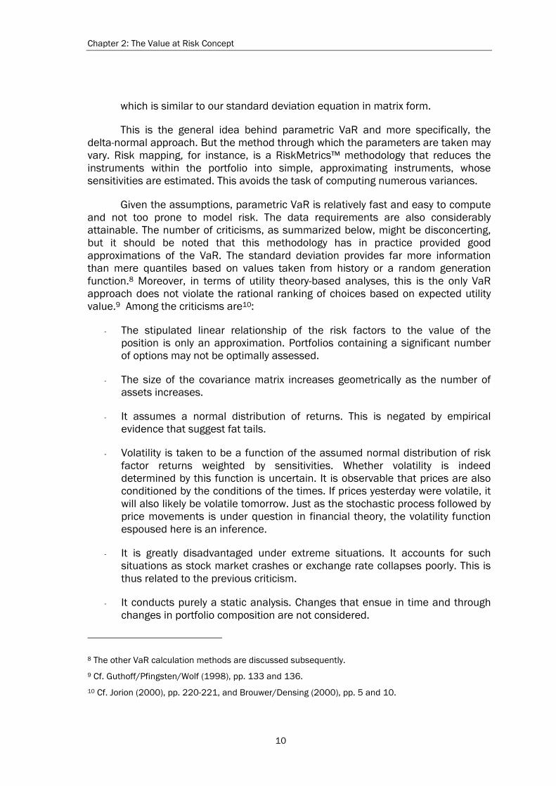
Γ+σ∆α−=σα−= . (14 )
Whether this is an efficient way of accounting for non-linearities stands however in question. Moreover, criticisms made against the delta-normal method could be extended to the delta-gamma method.
2.2.22.2.22.2.22.2.2 Historical SimulationHistorical SimulationHistorical SimulationHistorical Simulation
Historical simulation is a numerical approach at calculating the VaR of an asset or portfolio for a specified holding period and confidence level that takes past data on the movements of underlying risk factors to determine the probable returns. The whole calculation process arrives at a series of profit and loss figures. The value at the specified quantile is the absolute VaR.
If, for example, we want to calculate the VaR of a portfolio given a 95% confidence interval using a historical simulation of risk factor movements covering 100 days, then the historical simulation VaR would be the value of the 95th percentile of all the derived values. In other words, it is the 96th worst value of the portfolio returns we have calculated. To arrive at this, the risk factors are first of all inputted into the valuation formula of the portfolio to yield hypothetical mark-to-market values of the portfolio.12 This could include an exchange rate, an interest rate, etc. Meanwhile, the current value of the portfolio at the analysis date is also derived. This current value is then subtracted from each of the 100 historically simulated values. These are ranked from highest to lowest. The 96th worst value of the ranked values is the potential loss that should not be exceeded with 95% certainty.
The generalized procedure is as follows:13
1. Take a portfolio and determine its current value at the analysis date by inputting the actual parameters of the identified risk factors into the appropriate valuation formula.
2. Choose a confidence level and holding period for which the potential loss will be determined.
3. Take a set of historical risk factor values appropriate or significant for the holding period chosen. Input these historical values into the valuation formula
12 As these risk factor movements are actual data of the period in question, the process of incorporating them into the valuation function is called marking to market. 13 Cf. Linsmeier/Pearson (2000), p. 50.
Chapter 2: The Value at Risk Concept
13
of the portfolio. As a result, hypothetical mark-to-market values will be calculated.
4. Subtract the current value of the portfolio from the hypothetical mark-to-market values. This yields the profit and loss values of the portfolio.
5. Rank the profit and loss values. The value at the chosen confidence level is the VaR per historical simulation.
Historical simulation is relatively easy to implement and takes on a full valuation of all positions in its VaR computation, while using only one sample path. There is no modeling or approximation of some sort. But the calculation could quickly become complicated for large portfolios with complex structures. On the other hand, if the sample size is too small, then an estimation error could ensue. Another point against its credibility is the use of historical data to forecast future risk factor movements. It is assumed that historical risk factor movements would capture future risk factor movements, and thus, taking historical data is justifiable. There is an element of realism there, because historical trends could actually repeat. But taking a sample of values arbitrarily will also have its effects. The results depend heavily on the set of variables chosen. Moreover, an analyst is lucky if all values corresponding to the number of days chosen are all available.
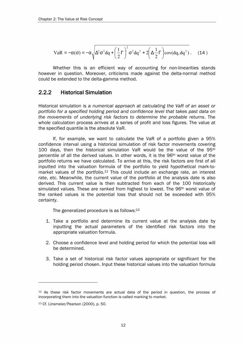
Example. The following concrete example is an adjusted version of the case given by Linsmeier/Pearson (2000), who illustrate the VaR calculation of a single, three-month foreign exchange (FX) forward contract.14 The analysis date is May 20, 2000. The forward contract requires a payment of 15 million US dollars on August 19, 2000, which is 91 days hence. In exchange, the company will receive 10 million pounds. The valuation formula is:
( ) ( ))360/91(r1
M15USD
)360/91(r1
M10GBPFX)X(V
USDGBP
USDGBP +
−
+⋅= , (15 )
where USDGBPFX is the USD/GBP FX rate, rGBP the British pound interest rate and
rUSD the US dollar interest rate.
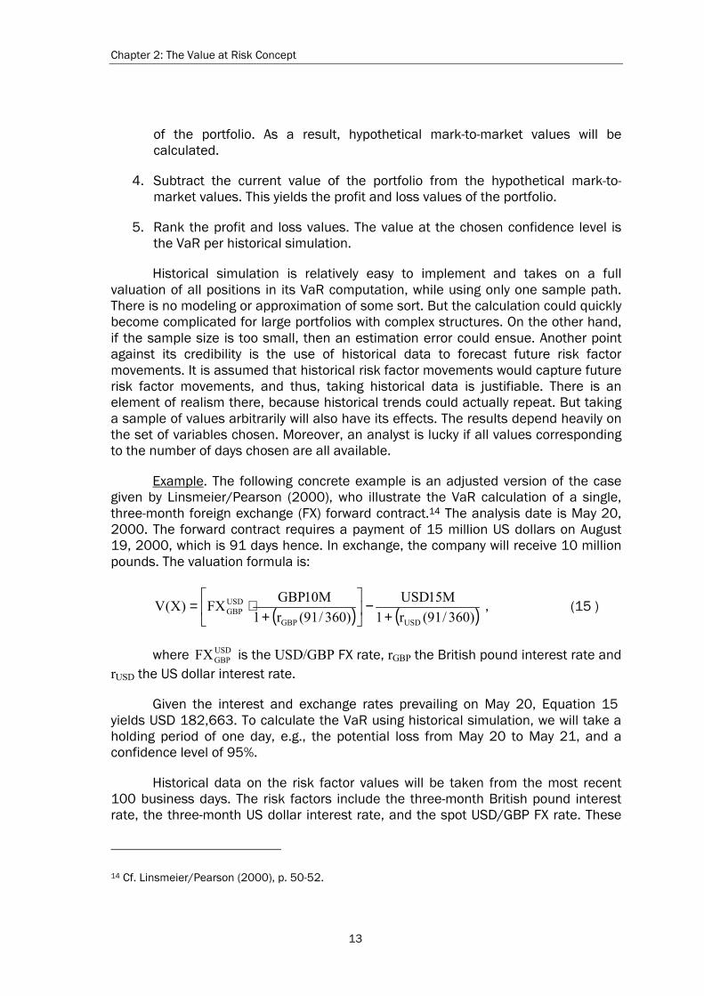
Given the interest and exchange rates prevailing on May 20, Equation 15 yields USD 182,663. To calculate the VaR using historical simulation, we will take a holding period of one day, e.g., the potential loss from May 20 to May 21, and a confidence level of 95%.
Historical data on the risk factor values will be taken from the most recent 100 business days. The risk factors include the three-month British pound interest rate, the three-month US dollar interest rate, and the spot USD/GBP FX rate. These
14 Cf. Linsmeier/Pearson (2000), p. 50-52.
Chapter 2: The Value at Risk Concept
14
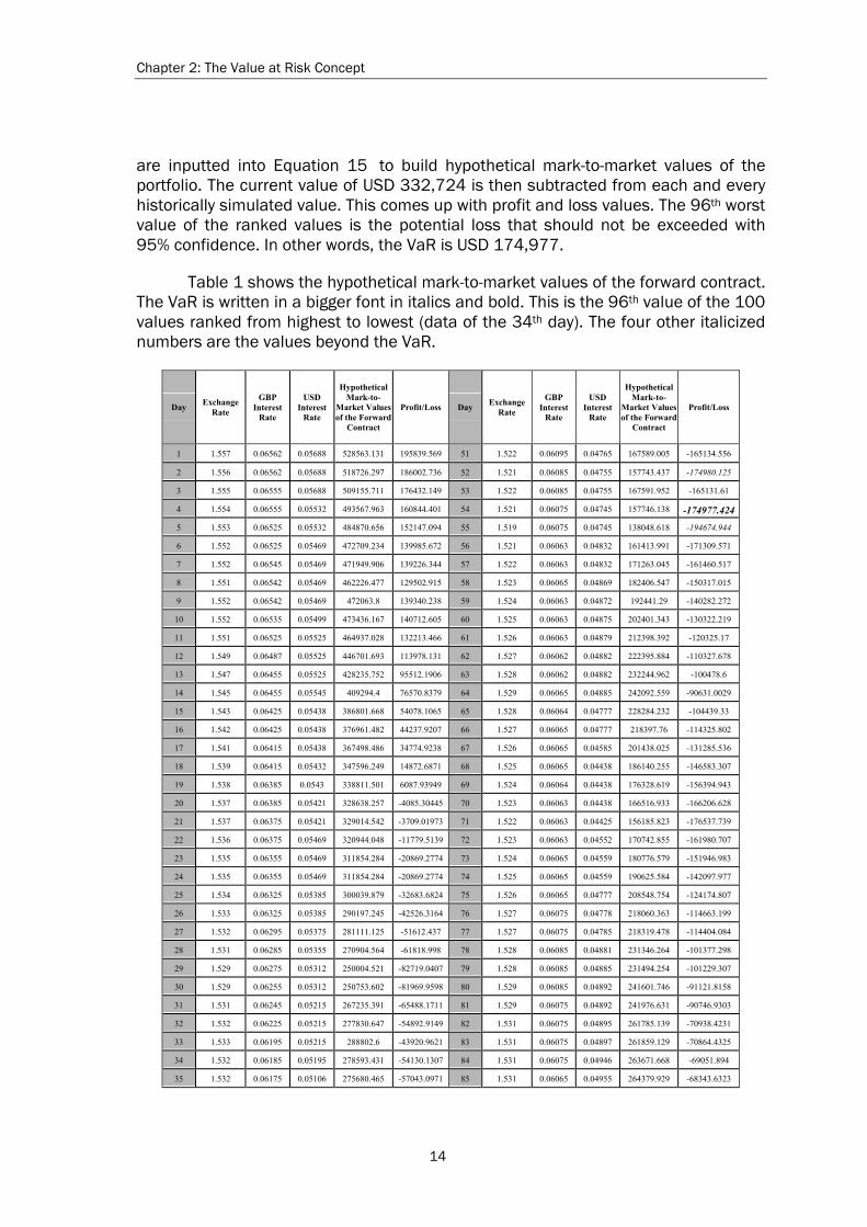
are inputted into Equation 15 to build hypothetical mark-to-market values of the portfolio. The current value of USD 332,724 is then subtracted from each and every historically simulated value. This comes up with profit and loss values. The 96th worst value of the ranked values is the potential loss that should not be exceeded with 95% confidence. In other words, the VaR is USD 174,977.
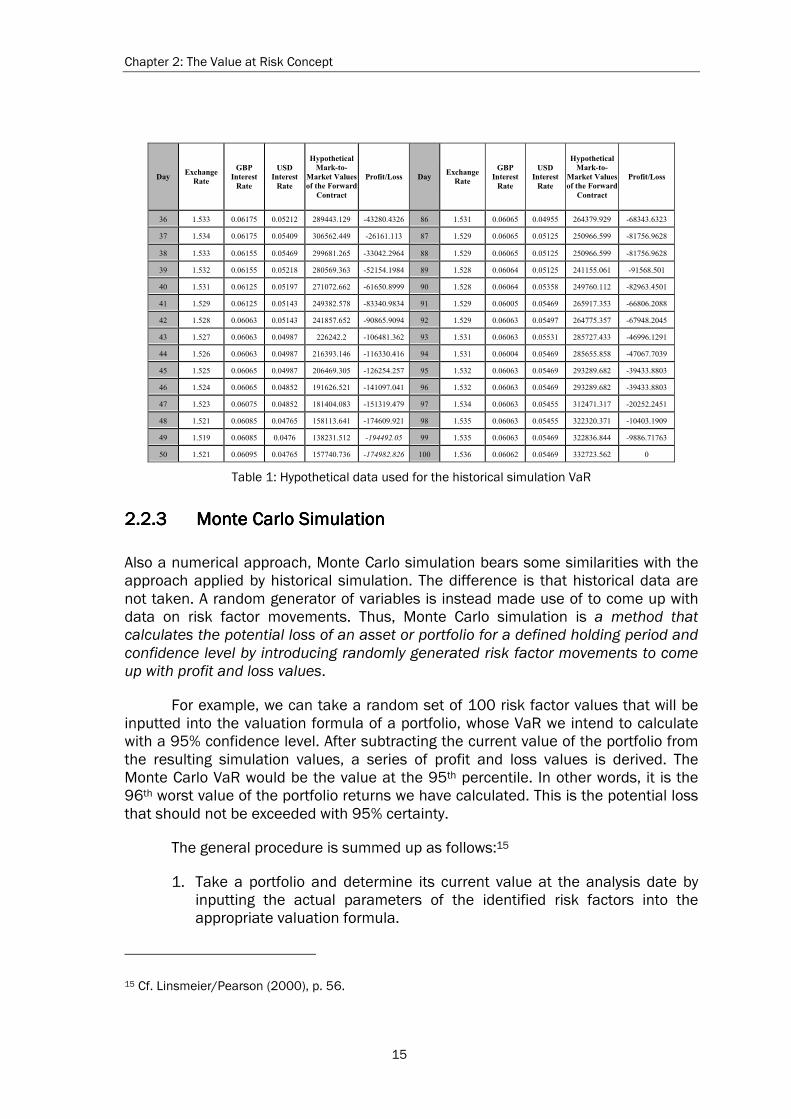
Table 1 shows the hypothetical mark-to-market values of the forward contract. The VaR is written in a bigger font in italics and bold. This is the 96th value of the 100 values ranked from highest to lowest (data of the 34th day). The four other italicized numbers are the values beyond the VaR.
Day Exchange
Rate
GBP Interest
Rate
USD Interest
Rate
Hypothetical Mark-to-
Market Values of the Forward
Contract
Profit/Loss Day Exchange
Rate
GBP Interest
Rate
USD Interest
Rate
Hypothetical Mark-to-
Market Values of the Forward
Contract
Profit/Loss
1 1.557 0.06562 0.05688 528563.131 195839.569 51 1.522 0.06095 0.04765 167589.005 -165134.556
2 1.556 0.06562 0.05688 518726.297 186002.736 52 1.521 0.06085 0.04755 157743.437 -174980.125
3 1.555 0.06555 0.05688 509155.711 176432.149 53 1.522 0.06085 0.04755 167591.952 -165131.61
4 1.554 0.06555 0.05532 493567.963 160844.401 54 1.521 0.06075 0.04745 157746.138 -174977.424
5 1.553 0.06525 0.05532 484870.656 152147.094 55 1.519 0.06075 0.04745 138048.618 -194674.944
6 1.552 0.06525 0.05469 472709.234 139985.672 56 1.521 0.06063 0.04832 161413.991 -171309.571
7 1.552 0.06545 0.05469 471949.906 139226.344 57 1.522 0.06063 0.04832 171263.045 -161460.517
8 1.551 0.06542 0.05469 462226.477 129502.915 58 1.523 0.06065 0.04869 182406.547 -150317.015
9 1.552 0.06542 0.05469 472063.8 139340.238 59 1.524 0.06063 0.04872 192441.29 -140282.272
10 1.552 0.06535 0.05499 473436.167 140712.605 60 1.525 0.06063 0.04875 202401.343 -130322.219
11 1.551 0.06525 0.05525 464937.028 132213.466 61 1.526 0.06063 0.04879 212398.392 -120325.17
12 1.549 0.06487 0.05525 446701.693 113978.131 62 1.527 0.06062 0.04882 222395.884 -110327.678
13 1.547 0.06455 0.05525 428235.752 95512.1906 63 1.528 0.06062 0.04882 232244.962 -100478.6
14 1.545 0.06455 0.05545 409294.4 76570.8379 64 1.529 0.06065 0.04885 242092.559 -90631.0029
15 1.543 0.06425 0.05438 386801.668 54078.1065 65 1.528 0.06064 0.04777 228284.232 -104439.33
16 1.542 0.06425 0.05438 376961.482 44237.9207 66 1.527 0.06065 0.04777 218397.76 -114325.802
17 1.541 0.06415 0.05438 367498.486 34774.9238 67 1.526 0.06065 0.04585 201438.025 -131285.536
18 1.539 0.06415 0.05432 347596.249 14872.6871 68 1.525 0.06065 0.04438 186140.255 -146583.307
19 1.538 0.06385 0.0543 338811.501 6087.93949 69 1.524 0.06064 0.04438 176328.619 -156394.943
20 1.537 0.06385 0.05421 328638.257 -4085.30445 70 1.523 0.06063 0.04438 166516.933 -166206.628
21 1.537 0.06375 0.05421 329014.542 -3709.01973 71 1.522 0.06063 0.04425 156185.823 -176537.739
22 1.536 0.06375 0.05469 320944.048 -11779.5139 72 1.523 0.06063 0.04552 170742.855 -161980.707
23 1.535 0.06355 0.05469 311854.284 -20869.2774 73 1.524 0.06065 0.04559 180776.579 -151946.983
24 1.535 0.06355 0.05469 311854.284 -20869.2774 74 1.525 0.06065 0.04559 190625.584 -142097.977
25 1.534 0.06325 0.05385 300039.879 -32683.6824 75 1.526 0.06065 0.04777 208548.754 -124174.807
26 1.533 0.06325 0.05385 290197.245 -42526.3164 76 1.527 0.06075 0.04778 218060.363 -114663.199
27 1.532 0.06295 0.05375 281111.125 -51612.437 77 1.527 0.06075 0.04785 218319.478 -114404.084
28 1.531 0.06285 0.05355 270904.564 -61818.998 78 1.528 0.06085 0.04881 231346.264 -101377.298
29 1.529 0.06275 0.05312 250004.521 -82719.0407 79 1.528 0.06085 0.04885 231494.254 -101229.307
30 1.529 0.06255 0.05312 250753.602 -81969.9598 80 1.529 0.06085 0.04892 241601.746 -91121.8158
31 1.531 0.06245 0.05215 267235.391 -65488.1711 81 1.529 0.06075 0.04892 241976.631 -90746.9303
32 1.532 0.06225 0.05215 277830.647 -54892.9149 82 1.531 0.06075 0.04895 261785.139 -70938.4231
33 1.533 0.06195 0.05215 288802.6 -43920.9621 83 1.531 0.06075 0.04897 261859.129 -70864.4325
34 1.532 0.06185 0.05195 278593.431 -54130.1307 84 1.531 0.06075 0.04946 263671.668 -69051.894
35 1.532 0.06175 0.05106 275680.465 -57043.0971 85 1.531 0.06065 0.04955 264379.929 -68343.6323
Chapter 2: The Value at Risk Concept
15
Day Exchange
Rate
GBP Interest
Rate
USD Interest
Rate
Hypothetical Mark-to-
Market Values of the Forward
Contract
Profit/Loss Day Exchange
Rate
GBP Interest
Rate
USD Interest
Rate
Hypothetical Mark-to-
Market Values of the Forward
Contract
Profit/Loss
36 1.533 0.06175 0.05212 289443.129 -43280.4326 86 1.531 0.06065 0.04955 264379.929 -68343.6323
37 1.534 0.06175 0.05409 306562.449 -26161.113 87 1.529 0.06065 0.05125 250966.599 -81756.9628
38 1.533 0.06155 0.05469 299681.265 -33042.2964 88 1.529 0.06065 0.05125 250966.599 -81756.9628
39 1.532 0.06155 0.05218 280569.363 -52154.1984 89 1.528 0.06064 0.05125 241155.061 -91568.501
40 1.531 0.06125 0.05197 271072.662 -61650.8999 90 1.528 0.06064 0.05358 249760.112 -82963.4501
41 1.529 0.06125 0.05143 249382.578 -83340.9834 91 1.529 0.06005 0.05469 265917.353 -66806.2088
42 1.528 0.06063 0.05143 241857.652 -90865.9094 92 1.529 0.06063 0.05497 264775.357 -67948.2045
43 1.527 0.06063 0.04987 226242.2 -106481.362 93 1.531 0.06063 0.05531 285727.433 -46996.1291
44 1.526 0.06063 0.04987 216393.146 -116330.416 94 1.531 0.06004 0.05469 285655.858 -47067.7039
45 1.525 0.06065 0.04987 206469.305 -126254.257 95 1.532 0.06063 0.05469 293289.682 -39433.8803
46 1.524 0.06065 0.04852 191626.521 -141097.041 96 1.532 0.06063 0.05469 293289.682 -39433.8803
47 1.523 0.06075 0.04852 181404.083 -151319.479 97 1.534 0.06063 0.05455 312471.317 -20252.2451
48 1.521 0.06085 0.04765 158113.641 -174609.921 98 1.535 0.06063 0.05455 322320.371 -10403.1909
49 1.519 0.06085 0.0476 138231.512 -194492.05 99 1.535 0.06063 0.05469 322836.844 -9886.71763
50 1.521 0.06095 0.04765 157740.736 -174982.826 100 1.536 0.06062 0.05469 332723.562 0
Table 1: Hypothetical data used for the historical simulation VaR
2.2.32.2.32.2.32.2.3 Monte Carlo SimulationMonte Carlo SimulationMonte Carlo SimulationMonte Carlo Simulation
Also a numerical approach, Monte Carlo simulation bears some similarities with the approach applied by historical simulation. The difference is that historical data are not taken. A random generator of variables is instead made use of to come up with data on risk factor movements. Thus, Monte Carlo simulation is a method that calculates the potential loss of an asset or portfolio for a defined holding period and confidence level by introducing randomly generated risk factor movements to come up with profit and loss values.
For example, we can take a random set of 100 risk factor values that will be inputted into the valuation formula of a portfolio, whose VaR we intend to calculate with a 95% confidence level. After subtracting the current value of the portfolio from the resulting simulation values, a series of profit and loss values is derived. The Monte Carlo VaR would be the value at the 95th percentile. In other words, it is the 96th worst value of the portfolio returns we have calculated. This is the potential loss that should not be exceeded with 95% certainty.
The general procedure is summed up as follows:15
1. Take a portfolio and determine its current value at the analysis date by inputting the actual parameters of the identified risk factors into the appropriate valuation formula.
15 Cf. Linsmeier/Pearson (2000), p. 56.
Chapter 2: The Value at Risk Concept
16
2. Choose a confidence level and holding period for which the potential loss will be determined.
3. Run the random generator and value the portfolio using a number of parameters that is appropriate for the holding period chosen. As a result, hypothetical values of the portfolio will be yielded.
4. Subtract the current value of the portfolio from the simulated values. This yields the profit and loss values of the portfolio.
5. Rank the profit and loss values. The value at the chosen confidence level is the VaR per Monte Carlo simulation.
This is said to be the most powerful method to compute the VaR. If non-linear relationships are involved in the portfolio, the use of Monte Carlo simulation will better accomplish the VaR estimation. If the number of variables were large enough, the resulting values would capture the profit and loss distribution well. Unlike other VaR analyses that provide only a static consideration of value changes, Monte Carlo simulation allows for dynamic developments in the variables as well as the portfolio composition. Moreover, we do not have a general assumption on the process followed by risk factor movements. Ergo, it is a very open and comprehensive approach in measuring market risk, if the modeling were correct. The calculation is however tedious (but less tedious than non-VaR-based methodologies). Since it involves several variables, it requires resources, e.g., computer power, that could tackle this effortlessly.16
The tabulated results of a Monte Carlo simulation could appear similar to the example given in Section 2.2.2. The factors used are however derived from a model.
2.32.32.32.3 Criticisms on VaRCriticisms on VaRCriticisms on VaRCriticisms on VaR
2.3.12.3.12.3.12.3.1 General EvaluationGeneral EvaluationGeneral EvaluationGeneral Evaluation
We have seen the different methodologies that may be used to arrive at the VaR. The strengths and weaknesses of such methodologies were touched upon briefly in the respective subsections. Before we conduct a general evaluation of the VaR, let us take a look at Table 2, which is a summary of the features of the discussed VaR approaches.
16 Cf. Jorion (2000), pp. 225-226 and Brouwer/Densing (2000), pp. 4-5.

Chapter 2: The Value at Risk Concept
17
Parametric VaR Historical Simulation
Monte Carlo Simulation
Holding period and confidence level
Determined as required by the analysis; results are thereby affected by the choice
Determined as required by the analysis; results are thereby affected by the choice
Determined as required by the analysis; results are thereby affected by the choice
Risk factor movements
Normally distributed Based on historical values
Based on a random generation function
VaR calculation The value at the specified quantile of the profit and loss distribution; the difference between the mean and the chosen quantile value of the assumed normal distribution.
The value at the specified quantile of the profit and loss distribution; the difference between the current value and the chosen quantile value of the historical distribution of values
The value at the specified quantile of the profit and loss distribution; the difference between the current value and the chosen quantile value of the simulated distribution of values
Communicability Easy Easy Easy
Level of difficulty of calculation
Easy; complication arises when the number of assets increase
Easy; complication arises for complex structures
Easy; complication arises for complex structures
Infrastructure/data requirements
Surmountable Surmountable Requires powerful calculation systems
Table 2: Summary of the features of VaR
This summary points out that VaR is generally an easily communicable risk figure. However, depending on the methodology followed to derive the figure and the chosen holding period and confidence level, the number always changes. Several studies have shown this. Assumptions on how the risk factors move are for instance critical. Historical values appear realistic. On the other hand, Monte Carlo simulation could capture better non-linear behavior, which cannot be efficiently captured by parametric VaR.
Ideally, the results of the different methodologies that take up a huge sample data for the same confidence level and holding period should converge. Huge discrepancies between parametric VaR and Monte Carlo simulation could be attributed to the non-consideration of non-linearities. On the other hand, discrepancies between historical simulation and a Monte Carlo simulation that adopts normally distributed risk factor movements could indicate a disparity of the assumed movements in Monte Carlo from the historical path of the values, which may be deemed more realistic.17
17 Cf. Bonvin (2000), p. 8.

Chapter 2: The Value at Risk Concept
18
History however need not give the right answer. VaR is often criticized as driving by looking mainly at the rearview mirror. Even adopted future scenarios are based on already reviewed past events.18
What VaR method to use is a decision of the analyzer. When it does not cost much time and effort, the use of all methodologies, whose results could then be compared against each other as a form of check and balance, is ideal.
2.3.22.3.22.3.22.3.2 Summative Evaluation from a Computational PerspectiveSummative Evaluation from a Computational PerspectiveSummative Evaluation from a Computational PerspectiveSummative Evaluation from a Computational Perspective
How non-linear components of a portfolio are not efficiently captured by parametric VaR has been pointed out in the previous section. This also holds true for historical simulation. Inability to capture non-linear behavior is actually one of the most relevant critiques that could be raised against VaR. Monte Carlo simulation however attempts to accomplish this. This is stated in Table 3, which summarizes the features of VaR as against some factors or criteria that imply mathematical considerations.
Parametric VaR Historical Simulation Monte Carlo SimulationMonte Carlo SimulationMonte Carlo SimulationMonte Carlo Simulation
Non-linear components
May be attempted to be captured by the delta-gamma approach, albeit insufficiently
Not captured Can be captured
Fat tails Not incorporated Can be accounted for Can be accounted for
Extreme scenarios Not considered Not considered Can be considered
Variations in time A static analysis; no portfolio composition or other changes over time
A static analysis; no portfolio composition or other changes over time
Could perform a dynamic analysis; changes over time may be covered
Table 3: Problematic factors related to mathematical considerations
Inability to capture non-linear behavior results logically to estimation errors. Along with this, if the assumed risk factor movements are wrong, then estimation errors can also naturally ensue. In the case of historical simulation, it is crucial that the sample size be representative of the period in study. As for Monte Carlo simulation, the data should considerably be close to reality.
As regards actual facts, several studies have claimed that reality points to the existence of fat tails in the distribution. Simulation techniques have the possibility of taking this into consideration. This is however problematic for parametric VaR. The correctness of assuming a normal distribution becomes questionable. The VaR derived from a normal distribution underestimates then the true VaR. The higher
18 Cf. Frey (2000).
Chapter 2: The Value at Risk Concept
19
number of observations on the left tail of a fat-tailed distribution points to a higher VaR.
Since the normal distribution assumption is doubtful, what follows is the question on the advisability of using correlation as a dependence measure. Correlation measurement is normally undertaken in a world of joint multivariate normal distributions and not for other distributions, which depict other phenomena such as fat tails.
Moreover, only Monte Carlo simulation can possibly efficiently capture extreme scenarios. Again, this statement is rooted in the fact that parametric VaR assumes normality. On the other hand, historical simulation only considers past scenarios, which need not include circumstances that go to the extremes. For this reason, the development and use of extreme value theory has ensued.
Variations in time are also important. At particular points, volatility may for example heavily increase. Static parametric analysis and historical simulation are not hereby ideal. McNeil and Frey (1999) have conducted research in this area.19 They have pointed out that historical simulation cannot distinguish between periods of high and low volatility. On the other hand, the assumption of normality made by parametric VaR, although yielding estimates that reflect current volatility, does not seem to hold for normal data.20 In line with portfolio component changes in time, only Monte Carlo simulation could reflect such changes in the analyses.
All in all, it appears that in consideration of the computational perspective, the Monte Carlo VaR gains ground against the other VaR methodologies. It does not however always observe the axioms of coherency. This will be discussed by the succeeding chapter.
19 They focus on conditional return distributions (conditioned on current volatility) and the marginal distribution of the stochastic volatility process. 20 Cf. McNeil/Frey (1999), p. 3.
Chapter 3Chapter 3Chapter 3Chapter 3 Value at Risk and CoherencyValue at Risk and CoherencyValue at Risk and CoherencyValue at Risk and Coherency
3.13.13.13.1 CoherencyCoherencyCoherencyCoherency
In spite of its drawbacks, VaR is the most popular market risk measurement technique. But aside from market risk, attempts have been made to capture credit risk via VaR-based methodologies. CreditMetrics of J.P. Morgan attempts for example to generate a profit and loss distribution for loans, such that a quantile may be selected to determine the credit-at-risk. The challenge is to come up with a single VaR figure for portfolios subject to market, credit and other risks. Modern risk management now demands for the integration of various risk factors into one VaR figure. The aim of the so-called integrated risk management is however not simple to achieve. Assumptions have to be made as to the distribution that the factors follow, correlations have to be adjusted into the figures, and aggregation obstacles related to the fact that the estimates are expressed in different units or are taken for different periods in time have to be overcome.
Due to the inherent complexity of the considerations to be made, chances are high that at critical points in the analysis, one could take a wrong turn. Artzner, Delbaen, Eber and Heath (1997, 1998) have proposed axioms that should be fulfilled by risk measures in order for them to be coherent in the aggregation process. Their main argument is: the risk measures ρ(X) and ρ(Y) derived for a pair of investments X and Y, dependent or not, given a total return R, and positive numbers λ and N, should fulfill the following properties:
Translation invariance ρ(X+ N • R) = ρ(X) - N (16 )
Subadditivity ρ(X + Y) < ρ(X)+ ρ(Y) (17 )
Positive homogeneity ρ(λ • X) = λ • ρ(X) (18 )
Monotonicity ρ(X) ≥ ρ(Y), if X < Y (19 )
As outlined by the above-mentioned academicians, these axioms of coherency convey the following:

Chapter 3: Value at Risk and Coherency
21
3.1.13.1.13.1.13.1.1 Translation InvariancTranslation InvariancTranslation InvariancTranslation Invariance e e e [ρ [ρ [ρ [ρ((((X+ + + + N • • • • R) = ) = ) = ) = ρ(ρ(ρ(ρ(X) ) ) ) N]
By adding a risk-free amount to the initial position X and investing it in the instrument in use, the risk measure will simply decrease by N. This is also referred to as the risk-free condition.
What does it mean when translation invariance does not hold? An additional risk-free investment will appear to add risk to the already existing position. The new investment will have a factor in it that makes the existing X behave differently when combined with it. Problems may for example occur in some insurance premium calculations, e.g., proportional risk loading.21
3.1.23.1.23.1.23.1.2 Subadditivity [Subadditivity [Subadditivity [Subadditivity [ρρρρ((((X + Y) ) ) ) <<<< ρ(ρ(ρ(ρ(X) ) ) ) + ρρρρ((((Y)])])])]
When we put two instruments together to form a portfolio, the total risk of the two together should not be above the sum of the individual risks of the instruments. In other words, the risk of X and Y together should be equal or less than the sum of the risk of X alone and the risk of Y alone.
If this did not hold, there are possible ways of taking advantage of it. For instance, an investor in an exchange would rather set up two separate accounts for two instruments instead of putting them together. In this way, he avoids a higher margin requirement. On the other hand, a firm would break up its business into two in order to reduce its capital adequacy requirement. Regulatory authorities namely impose capital requirements on the basis of the firms market risk exposures.
But over and beyond regulatory concerns, subadditivity also has its relevance in risk management. If the risks of two desks have been calculated independently and if subadditivity holds, then one could just add the two individually derived risks together. This would then indicate the total risk. Subadditivity then allows for a decentralized calculation of the risks of various positions taken within the firm, which may then be simply aggregated.
3.1.33.1.33.1.33.1.3 Positive Homogeneity Positive Homogeneity Positive Homogeneity Positive Homogeneity [[[[ρρρρ((((λλλλ • • • • X) = ) = ) = ) = λλλλ • • • • ρρρρ((((X)])])])]
Whereas subadditivity implies lower risk figures for composite positions, this axiom states that the size of a position does not directly affect its risk. For all λ ≥ 0, risk is scalar multiplicative. The risk measure peculiar to X remains the same and will just have to be multiplied by λ as the size of the position increases.
21 This has been identified by Delbaen in correspondence.
Chapter 3: Value at Risk and Coherency
22
This confirms that there is no imposed restriction on any firm or investor to take the same position in whatever instrument. Each takes a position choice according to his capacity. Increased position in an instrument does not induce incremental risk. Liquidity is assumed.
What is the relevance of positive homogeneity? Similar to translation invariance, the derived risk measure should already capture the fundamental risk elements faced by an instrument. To arrive at its multiple, the figures will just have to be scaled. If size were a factor, then this will have its consequence on the speed of liquidation, among others. Such will then have to be factored in. It will be definitely unreasonable to impose this condition, if position size directly affects risk.22
3.1.43.1.43.1.43.1.4 Monotonicity [Monotonicity [Monotonicity [Monotonicity [ρρρρ((((X) ) ) ) ≥≥≥≥ ρρρρ((((Y), if ), if ), if ), if X <<<< Y]]]]
In analyzing positive homogeneity, we have been dealing with positions of the same reference instrument. Monotonicity compares two different instruments. If X < Y, it follows that ρ(X) ≥ ρ(Y). The risk faced by an instrument with lower returns is greater than that of another instrument with higher returns. If X = 10 and Y = 20, then the risk measure ρ(X) is greater than the risk measure ρ(Y).
What is the relevance of monotonicity? Monotonicity upholds the returns of an instrument as an ordering determinant of risk ranking between instruments. If this did not hold, we will not be able to rank instruments in terms of their risks. Comparability of risk measures meanwhile denotes the possibility of risk aggregation.
Note that this axiom rules out standard deviations and its multiples as risk measures.
Given all these axioms, we can then proceed to investigate the coherency of the different VaR approaches. Once they are adhered to, then the approach may be declared coherent.
3.23.23.23.2 The Coherency of VaRThe Coherency of VaRThe Coherency of VaRThe Coherency of VaR
VaR is not coherent at all times. Although some analyses involving selected instruments satisfy the axioms of coherency, others do not. The following section will conduct an analysis of the coherency of different VaR methodologies.
22 Cf. Gaese (1999), p. 56.

Chapter 3: Value at Risk and Coherency
23
3.2.13.2.13.2.13.2.1 The Coherency of Parametric VaR (DeltaThe Coherency of Parametric VaR (DeltaThe Coherency of Parametric VaR (DeltaThe Coherency of Parametric VaR (Delta----Normal)Normal)Normal)Normal)
3.2.1.1 Translation Invariance
Translation invariance holds for delta-normal VaR calculations. The underlying idea is that the standard deviation changes in accordance with any added risk-free amount. A smaller VaR results.
3.2.1.2 Subadditivity
If the VaR is computed using a distribution that has all prices in a joint normal distribution, then the quantile measure will satisfy the subadditivity axiom, for as long as we have a confidence level above 50%.23 In a joint distribution, the correlations are accounted for. Thus, parametric VaR that takes on a joint multivariate normal distribution of risk factors will not have any problems with subadditivity.
VaR in general is actually coherent for as long as we are dealing with multivariate normal distributions or more specifically, elliptical distributions.24 For any two portfolios with given VaR figures ρ(X) and ρ(Y), the sum of the two figures will always be greater than ρ(X+Y). Note that ρ(X), ρ(Y) and ρ(X+Y) have distributions of the same type such that the data in Table 4 holds.
VaR (X) µ + ασx
VaR (Y) µ + ασY
VaR (X + Y) E(X+Y) + α[σ(X+Y)]
VaR (X + Y) = VaR (X) + VaR (Y)
Table 4: Subadditivity of the parametric VaR of elliptical distributions
3.2.1.3 Positive Homogeneity
Will scaling a stock position X by 2 come up with the same value as the VaR of stock position X multiplied by 2? Yes. We arrive at the same figure. See Table 5 for details on an example of a bond with a known standard deviation of 0.95%. On the left side of Table 5, we double the position first. The standard deviation remains to be 0.95%. Thus, the VaR assuming a one-day holding period and a confidence level of 95% will lie at -1.5675% (=-1.65*0.0095); that is, the VaR is SFr. -3,135.00 (=-1.5675% * 200,000). This is exactly equal to multiplying the VaR of position X by 2 as indicated on the right side of the table:
23 Cf. Artzner/Delbaen/Eber/Heath (1998), p. 14 and Studer (1997), p. 20. 24 Cf. Embrechts/McNeil/Straumann (1999), pp. 12-13.
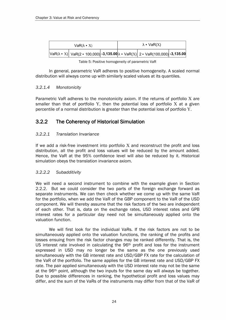
Chapter 3: Value at Risk and Coherency
24
VaR(λ • X) λ • VaR(X)
VaR(λ • X) VaR(2 • 100,000) -3,135.00 λ • VaR(X) 2 • VaR(100,000) -3,135.00
Table 5: Positive homogeneity of parametric VaR
In general, parametric VaR adheres to positive homogeneity. A scaled normal distribution will always come up with similarly scaled values at its quantiles.
3.2.1.4 Monotonicity
Parametric VaR adheres to the monotonicity axiom. If the returns of portfolio X are smaller than that of portfolio Y, then the potential loss of portfolio X at a given percentile of a normal distribution is greater than the potential loss of portfolio Y.
3.2.23.2.23.2.23.2.2 The Coherency of Historical SimulationThe Coherency of Historical SimulationThe Coherency of Historical SimulationThe Coherency of Historical Simulation
3.2.2.1 Translation Invariance
If we add a risk-free investment into portfolio X and reconstruct the profit and loss distribution, all the profit and loss values will be reduced by the amount added. Hence, the VaR at the 95% confidence level will also be reduced by it. Historical simulation obeys the translation invariance axiom.
3.2.2.2 Subadditivity
We will need a second instrument to combine with the example given in Section 2.2.2. But we could consider the two parts of the foreign exchange forward as separate instruments. We can then check whether we come up with the same VaR for the portfolio, when we add the VaR of the GBP component to the VaR of the USD component. We will thereby assume that the risk factors of the two are independent of each other. That is, data on the exchange rates, USD interest rates and GPB interest rates for a particular day need not be simultaneously applied onto the valuation function.
We will first look for the individual VaRs. If the risk factors are not to be simultaneously applied onto the valuation functions, the ranking of the profits and losses ensuing from the risk factor changes may be ranked differently. That is, the US interest rate involved in calculating the 96th profit and loss for the instrument expressed in USD may no longer be the same as the one previously used simultaneously with the GB interest rate and USD/GBP FX rate for the calculation of the VaR of the portfolio. The same applies for the GB interest rate and USD/GBP FX rate. The pair applied simultaneously with the USD interest rate may not be the same at the 96th point, although the two inputs for the same day will always be together. Due to possible differences in ranking, the hypothetical profit and loss values may differ, and the sum of the VaRs of the instruments may differ from that of the VaR of

Chapter 3: Value at Risk and Coherency
25
X and Y together. The VaR of the GBP component comes up to 148,594. The VaR of the USD component, on the other hand, is equal to -2,324. The sum of the two together is then equal to 150,918. Will this equal the VaR of the portfolio of the two together (without considering the instrument as a forward)? The VaR of the portfolio is equal to -122,578. Taking the absolute value of the terms, this respects subadditivity, as summarized in Table 6.
VaR(GBP) 148,594
VaR(USD) 2,324
VaR(GBP) + VaR(USD) 150,918
VaR(GBP+USD) 122,578
VaR (GBP + USD) < VaR (GBP) + VaR (USD)
Table 6: Subadditivity of the VaR per historical simulation
If that holds, then we can in a decentralized case add the VaRs of two instruments to come up with portfolio VaR. We are assured that the sum will always be greater than or equal to the true portfolio VaR. But due to the arbitrariness of the rankings, it is probable that there will be times at which subadditivity will not be respected. Historical VaR comes up with a percentile-based VaR that does not take into consideration a joint distribution of risk factors. Thus, it is possible that it will occasionally not satisfy subadditivity.
Artzner, Delbaen, Eber and Heath (1998) show how VaR may violate subadditivity in the case of instruments with exactly the same independently distributed distributions. They have the same density 0.90 on the interval [0,1], and the same density 0.05 on the interval [-2,0]. Both have positive expected values. If we take the individual 10% VaRs and sum them up, then we have a VaR of 0, since the 10% VaR of X and 10% VaR of Y are both equal to 0. But then, if we put X and Y together in a joint distribution, we can arrive at a VaR that is greater than 0.25 This violates subadditivity. See Table 7.
VaR (X) 0
VaR (Y) 0
VaR (X) + Var(Y) 0
But VaR (X + Y) > 0
VaR (X + Y) > VaR (X) + VaR (Y)
Table 7: Violation of subadditivity of percentile VaR
25 Cf. Artzner/Delbaen/Eber/Heath (1998), p. 14.
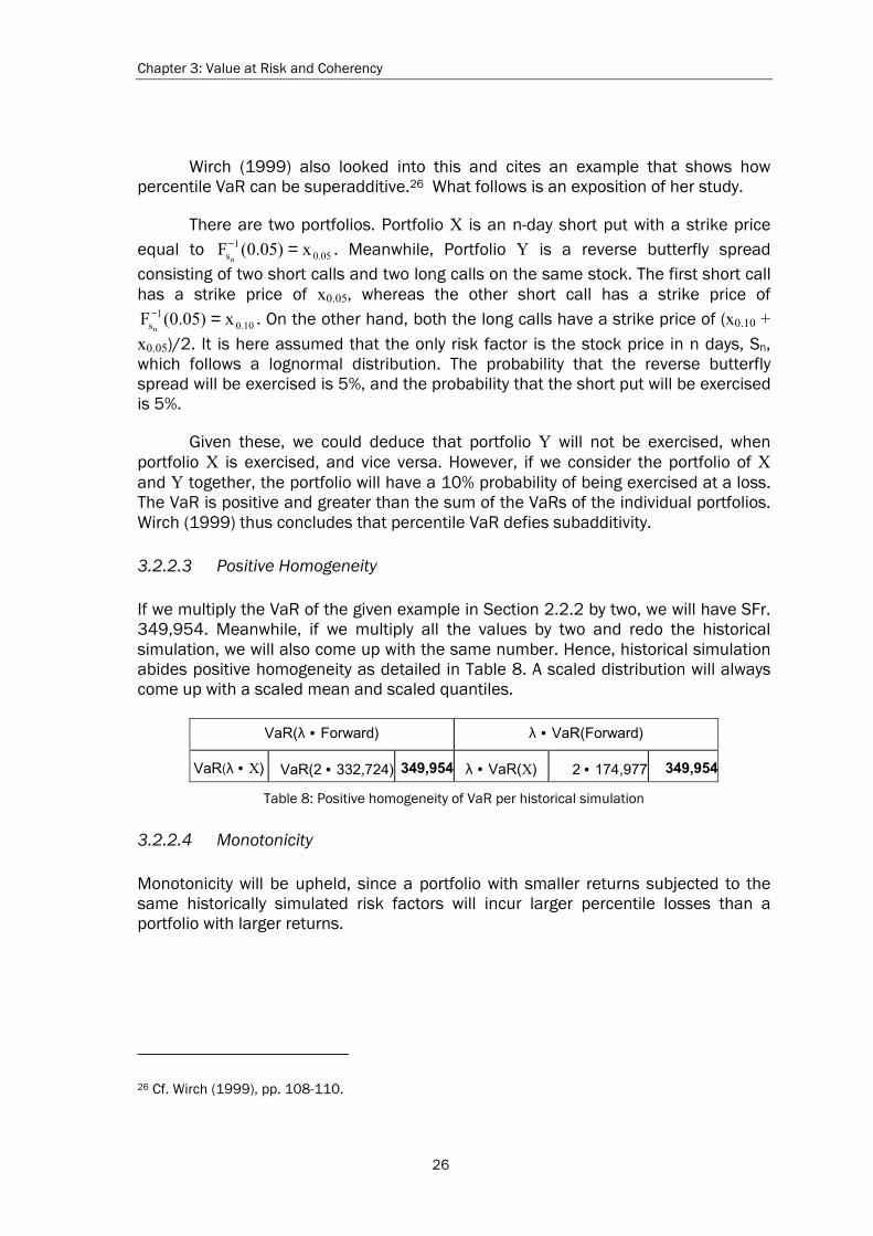
Chapter 3: Value at Risk and Coherency
26
Wirch (1999) also looked into this and cites an example that shows how percentile VaR can be superadditive.26 What follows is an exposition of her study.
There are two portfolios. Portfolio X is an n-day short put with a strike price equal to 05.0
1s x)05.0(F
n=− . Meanwhile, Portfolio Y is a reverse butterfly spread
consisting of two short calls and two long calls on the same stock. The first short call has a strike price of x0.05, whereas the other short call has a strike price of
10.01
s x)05.0(Fn
=− . On the other hand, both the long calls have a strike price of (x0.10 +
x0.05)/2. It is here assumed that the only risk factor is the stock price in n days, Sn, which follows a lognormal distribution. The probability that the reverse butterfly spread will be exercised is 5%, and the probability that the short put will be exercised is 5%.
Given these, we could deduce that portfolio Y will not be exercised, when portfolio X is exercised, and vice versa. However, if we consider the portfolio of X and Y together, the portfolio will have a 10% probability of being exercised at a loss. The VaR is positive and greater than the sum of the VaRs of the individual portfolios. Wirch (1999) thus concludes that percentile VaR defies subadditivity.
3.2.2.3 Positive Homogeneity
If we multiply the VaR of the given example in Section 2.2.2 by two, we will have SFr. 349,954. Meanwhile, if we multiply all the values by two and redo the historical simulation, we will also come up with the same number. Hence, historical simulation abides positive homogeneity as detailed in Table 8. A scaled distribution will always come up with a scaled mean and scaled quantiles.
VaR(λ • Forward) λ • VaR(Forward)
VaR(λ • X) VaR(2 • 332,724) 349,954 λ • VaR(X) 2 • 174,977 349,954
Table 8: Positive homogeneity of VaR per historical simulation
3.2.2.4 Monotonicity
Monotonicity will be upheld, since a portfolio with smaller returns subjected to the same historically simulated risk factors will incur larger percentile losses than a portfolio with larger returns.
26 Cf. Wirch (1999), pp. 108-110.

Chapter 3: Value at Risk and Coherency
27
3.2.33.2.33.2.33.2.3 The Coherency of Monte Carlo SimulationThe Coherency of Monte Carlo SimulationThe Coherency of Monte Carlo SimulationThe Coherency of Monte Carlo Simulation
3.2.3.1 Translation Invariance
Adding a risk-free investment into the portfolio should reduce the profit and loss values by as much as the added investment, such that to calculate the Monte Carlo VaR, one will just have to subtract the amount of the risk-free investment from the derived VaR. The Monte Carlo method does not employ a calculation procedure that obstructs translation invariance.
3.2.3.2 Subadditivity
The arguments raised for the superadditivity of percentile VaR as discussed in Section 3.2.2.2 continue to apply for Monte Carlo simulation. To illustrate its case differently, we will take an example that specifies a specific function or distribution that the risk factor movements will follow, as this is what the Monte Carlo approach fundamentally undertakes.
Studer (1997) does this in considering two portfolios X and Y with specifications on the profit and loss function. Portfolio X has a profit and loss function expressed as 2
1X qv −= . This means that it does not have positions in the second risk factor q2. Portfolio Y, meanwhile, has a profit and loss function expressed as 2
2Y qv −= . This means it does not have any positions in the first risk factor q1. As the two risk factors are independent and standard normally distributed, the profit and loss functions of X and Y are both q2-distributed with one degree of freedom, such that the VaR of X and the VaR of Y at 75% both lie at 1.32. However, the VaR of the composite portfolio, which is also q2-distributed, has its 75% VaR at 2.77. That means, the absolute value of the VaR of the portfolio exceeds that of the sum of the individual VaRs.27 Subadditivity is in this case violated.
3.2.3.3 Positive Homogeneity
This should be respected without any problem. Scaling the variables applied to the profit and loss function will also magnify the VaR in the same degree.
3.2.3.4 Monotonicity
Monotonicity will be upheld. A portfolio with smaller returns subjected to the same randomly generated risk factors will incur larger percentile losses than a portfolio with larger returns.
27 Cf. Studer (1997), p. 20.
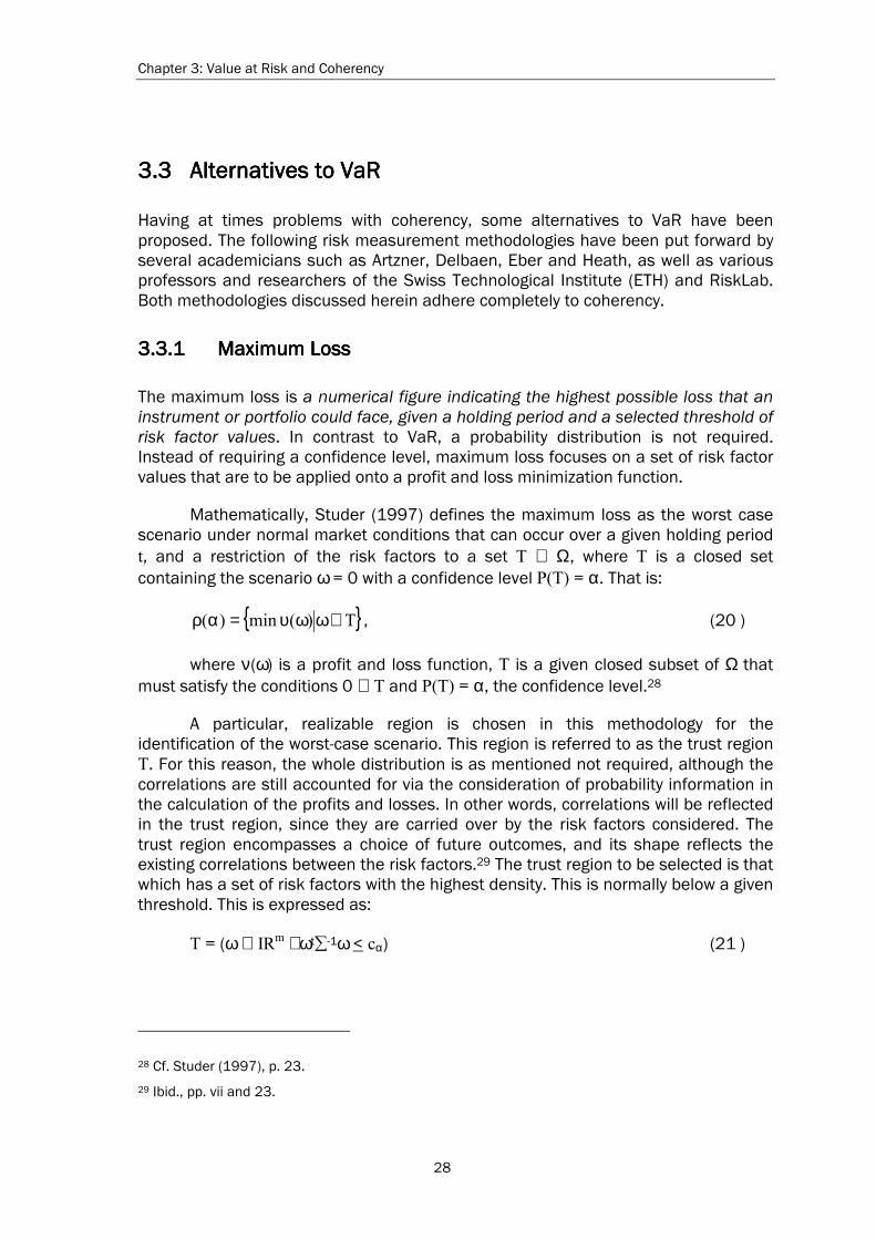
Chapter 3: Value at Risk and Coherency
28
3.33.33.33.3 Alternatives to VaRAlternatives to VaRAlternatives to VaRAlternatives to VaR
Having at times problems with coherency, some alternatives to VaR have been proposed. The following risk measurement methodologies have been put forward by several academicians such as Artzner, Delbaen, Eber and Heath, as well as various professors and researchers of the Swiss Technological Institute (ETH) and RiskLab. Both methodologies discussed herein adhere completely to coherency.
3.3.13.3.13.3.13.3.1 Maximum LossMaximum LossMaximum LossMaximum Loss
The maximum loss is a numerical figure indicating the highest possible loss that an instrument or portfolio could face, given a holding period and a selected threshold of risk factor values. In contrast to VaR, a probability distribution is not required. Instead of requiring a confidence level, maximum loss focuses on a set of risk factor values that are to be applied onto a profit and loss minimization function.
Mathematically, Studer (1997) defines the maximum loss as the worst case scenario under normal market conditions that can occur over a given holding period t, and a restriction of the risk factors to a set T ⊆ Ω, where T is a closed set containing the scenario ω = 0 with a confidence level P(T) = α. That is:
T)(min)( ∈ωωυ=αρ , (20 )
where ν(ω) is a profit and loss function, T is a given closed subset of Ω that must satisfy the conditions 0 ∈ T and P(T) = α, the confidence level.28
A particular, realizable region is chosen in this methodology for the identification of the worst-case scenario. This region is referred to as the trust region T. For this reason, the whole distribution is as mentioned not required, although the correlations are still accounted for via the consideration of probability information in the calculation of the profits and losses. In other words, correlations will be reflected in the trust region, since they are carried over by the risk factors considered. The trust region encompasses a choice of future outcomes, and its shape reflects the existing correlations between the risk factors.29 The trust region to be selected is that which has a set of risk factors with the highest density. This is normally below a given threshold. This is expressed as:
T = (ω ∈ IRm ω t-1ω < cα) (21 )
28 Cf. Studer (1997), p. 23. 29 Ibid., pp. vii and 23.
Chapter 3: Value at Risk and Coherency
29
where m is the degree of freedom and cα is a selected quantile or threshold value.30
Note the similarity of the proposed condition to that of parametric VaR.
Maximum loss is a step further than VaR in that it can efficiently surpass risk measurement difficulties for portfolios with non-linear relationships. In comparison to VaR, the determination of the maximum loss is however a tedious task. Knowledge of the algorithms involved in its calculation will not belong to common knowledge. Even with the calculation of VaR, the danger that some assumptions or fundamental considerations will be overlooked exists. The danger is even greater with maximum loss. Moreover, the build-up of the worst-case scenario appears to be quite critical in this approach. Whether it is going to be an adequate basis should be carefully scrutinized.
As regards the aggregation of risks, the maximum loss methodology comes up with a risk measure that can be surely aggregated. This has been extensively studied by Studer (1997). The methodology, in its basic form, lays down the possibility of deriving estimates of the incremental risk of single trades. On the basis of the maximum loss figure, we could come up with information on what risk factors would be most influential to the value of an instrument or portfolio.31 Moreover, just like VaR, it is possible to express the risk measure as a linear function of the portfolio risk.32 This means that the portfolio risk is comprised of risk components that have been added together, under the assumption of a linear relationship.
The key to the aggregation of the risk factors of the selected trust region is an algorithm called Levenberg-Marquardt.33 To keep the discussion simple, we could encapsulate the process as that of deriving a one-dimensional variable υ for a worst-case scenario for every risk factor. All υs are additive, since they are of the same common unit, e.g., profit/loss, and take correlations into consideration. Having obtained one-dimensional profit and loss values that is, having been able to aggregate one could then construct the profit and loss function and then look at the value at the chosen confidence level.34 This is then the maximum loss of the instrument, portfolio or institution.
Depending on the desired risk measure, we can undertake the analysis at different levels: instrument, portfolio or institution. If necessary, we could then also look into specific risks for a given level in a second model that includes risk factors
30 Ibid., p. 52. 31 Ibid., pp. 23 and 26. 32 Ibid., pp. 3 and 43-44. 33 For details into this algorithm, see Studer (1997), pp. 46-47. 34 An example is provided by Studer (1997) in connection with previous discussions in p. 48.

Chapter 3: Value at Risk and Coherency
30
pertaining to this specific level.35 The aggregation is then across risk categories and not across institutional levels. But the maximum loss of institutional levels could also be added to build the total maximum loss of a firm, since the measure is subadditive.
As regards coherency, the maximum loss methodology is a coherent risk measure and respects correlations for both linear and quadratic portfolios. Refer to Studer (1997) for proof on the coherency of the maximum loss methodology. Note however that he has gone further as to set up the axioms of coherency in the context of deriving the capital requirement to cover market risk exposures. The axioms of subadditivity and positive homogeneity are put together with an axiom on negativity and symmetry to build up the axioms on weak coherency, which are fulfilled by maximum loss.
3.3.23.3.23.3.23.3.2 Expected ShortfallExpected ShortfallExpected ShortfallExpected Shortfall
The expected shortfall is a numerical figure indicating the average of the possible losses that could be incurred beyond a selected tolerance level. Various literature refer to this as the tail conditional expectation, conditional loss or tail loss.
Taking the expected shortfall implies a selection of a benchmark value. The values beyond this benchmark value are then averaged to come up with the expected shortfall. That is:
[ ])X(VaRXXE)X( α≤−=ρ . (22 )
The condition hereby specifies X values that are below the quantile VaRα.36
Similar to VaR and maximum loss, a given value at a particular quantile plays a central role in the calculation, albeit with different underlying considerations. Moreover, unlike VaR and similar to maximum loss, the whole distribution of values is not required. Only the values lying beyond a target value are relevant.
In statistical terms, the expected shortfall is referred to as the lower partial moment37 of the first order. It can also be expressed as:
( ) ( ) −=ρ ∞−B )R(dFRBX , (23 )
where B is the target or benchmark value and F(R) is a function of profits and losses.38 Its being the moment of the first order is indicated by the fact that the
35 Cf. Studer (1997), p. 26. 36 Cf. Artzner/Delbaen/Eber/Heath (1997), p. 68 and Overbeck/Stahl (1998), p. 101. 37 Partial moments are integrations encompassing a selected part of the whole set of states Ω. 38 Cf. Matthes/Schröder (1998), p. 149.

Chapter 3: Value at Risk and Coherency
31
weighting of the risk measure is based on (B-R)1. That is, the enclosed terms being raised to the power 1 indicates its being of the first order.
Graphically, the expected shortfall is the average of the striped area in Figure 4. The area itself is the shortfall risk area. Incurring a shortfall is thereby understood as falling below a targeted level of profits/losses or returns.
Figure 4: Expected Shortfall
B, as said, is the benchmark value. This could for instance be the VaR. The values lying to the left of B are then taken to come up with the expected shortfall.
The methodology is simple. The advantage it has over VaR is that the results would reflect the gravity of the losses faced above a set target. VaR, on the other hand, specifies only a potential loss figure that would occur at a given confidence level. It does not inform us anymore about the potential size of the loss beyond this confidence level, if a loss ever occurs beyond the VaR figure.39 Jorion (2000) however states on the basis of an empirical study that the difference between VaR and expected shortfall diminishes as the confidence level of the analysis is increases.40
Expected shortfall does not however exactly capture risk behavior. The expected value results from the probabilities of losses. Small probabilities for big losses may in terms of expected shortfall be equal to small losses with higher probabilities. One should be more cautious of big losses even though they have lower
39 Cf. McNeil/Frey (1999), p. 13. 40 Cf. Jorion (2000), p. 99.
µ
Expected Shortfall
Returns B
Shortfall area
E(X) =
Chapter 3: Value at Risk and Coherency
32
probabilities. Moreover, just like delta-normal VaR, expected shortfall is a linear measurement methodology.41 It is also an instantaneous consideration of values.
Nevertheless, the fact that this risk measure is taken from a generalized scenario is cited by Artzner/Delbaen/Eber and Heath (1998) to be its best feature. A generalized scenario is a non-empty set of probability measures of the occurrence of a certain value. This is different from a simulation in that a generalized scenario is comprised of point masses chosen by the analyzer. Simulation data is chosen at random, in accordance with a predetermined distribution function. A risk measure derived from a general scenario is always coherent.42 That is, it satisfies the axioms of coherency.
The expected shortfall methodology actually encompasses the total potential loss of an instrument, portfolio or institution. This means that under a given general scenario, the risk measure can be determined for an instrument, portfolio or institution. There is no problem as to the attainment of a single risk figure. It could come up with an aggregate risk measure. But whether the calculated expected shortfall of a given investment X and investment Y could be added together to arrive at the total expected shortfall of the portfolio of both enters the realm of the investigation on its subadditivity. The following subsections will look into the adherence of expected shortfall to the axioms of coherency.
3.3.2.1 Translation Invariance
Translation invariance is respected because subtracting N from the mean arrives at a value equal to the expected negative value of a set of variables together with risk-free N.
3.3.2.2 Subadditivity
The sum of the negative expected values of two instruments will be equal to the sum of the expected negative value of a portfolio of these two instruments. Working on the example provided by Guthoff, Pfingsten and Wolf (1998), we see that subadditivity is respected. The addition of the expected losses of two portfolios, X and Y, is equal to the expected loss of the two instruments put together. The data is summarized in Table 9. The benchmark value is equal to -2.4. The expected shortfall (LPM1) of each instrument in the portfolio is weighted by its probability of occurrence. The total probability of occurrence does not exceed 5%.
41 Cf. Franzetti (1998), pp. 75-76 and 79. 42 Cf. Artzner/Delbaen/Eber/Heath, pp. 9-10 and 17.

Chapter 3: Value at Risk and Coherency
33
Value Shortfall from Benchmark =
-2.4
Probability of Occurrence
Lower Partial Moment One
X X1 = - 5 - 2.6 0.50% - 0.013
X2 = - 4 - 1.6 1.00% - 0.016
X3 = - 3 - 0.6 1.50% - 0.009
Total: -0.038
Y Y1 = - 5 - 2.6 1.00% -0.026
Y2 = - 4 - 1.6 0.50% -0.008
Y3 = - 3 - 0.6 1.00% -0.006
Total : -0.040
Table 9: Data on portfolios X and Y
To satisfy subadditivity, the expected shortfall of the portfolio of X and Y together should be smaller than or equal to the sum of the expected shortfall of the individual portfolios X and Y. That is, the sum of 0.038 and 0.04 should be greater than or equal to the expected shortfall of the portfolio of X and Y together. Fortunately, this holds true. The measure is subadditive. Adding the probabilities of occurrence together to come up with the expected shortfall of each instrument, we come up with a total expected shortfall of 0.078, which is also the sum of the individual expected shortfalls of the two instruments. See Table 10 and Table 11 for details.
Value Shortfall from Benchmark =
-2.4
Probability of Occurrence
Lower Partial Moment One
PFX + Y X1 + Y1 = - 5 - 2.6 1.50% - 0.039
X2 + Y2 = - 4 - 1.6 1.50% - 0.024
X3 + Y3 = - 3 - 0.6 2.50% - 0.015
Total: -0.078
Table 10: Expected shortfall of the portfolio of X and Y together
LPM1 (X) - 0.038
LPM1(Y) - 0.040
LPM1 (X) + LPM1(Y) - 0.078
LPM1 (X + Y) - 0.078
LPM1 (X + Y) = LPM1 (X) + LPM1 (Y)
Table 11: Subadditivity of expected shortfall
Chapter 3: Value at Risk and Coherency
34
3.3.2.3 Positive Homogeneity
Scaling the expected value is equal to scaling the variables involved by the same factor and deriving their mean. This may be proved just by looking into the properties of expected values; that is,
)X(E)X(E •λ=•λ . (24 )
The expected value of a variable X multiplied by a constant λ is equal to the constant multiplied by the expected value of the variable.43
3.3.2.4 Monotonicity
If X > Y, then the mean of the losses of X against the same reference probability distribution will be smaller than that of Y.
43 Cf. Copeland/Weston (1992), p. 148.

Chapter 4Chapter 4Chapter 4Chapter 4 CONCLUSIONCONCLUSIONCONCLUSIONCONCLUSION
Deriving a single risk measure for a firm is difficult. Even the consideration of just two market risk factors is laden with complexity, depending on the instrument taken. What methodology to use for risk measurement is then a decision that has to be carefully made. The axioms of coherency are helpful in this regard so as to determine whether the risk measure derived from a methodology would be sound. For instance, if a portfolio indeed has its diversification effect, this should be reflected by the risk measure too.
But choosing an appropriate risk measurement methodology should not just be based on the satisfaction of the axioms of coherency. Although subadditivity is indeed a relevant consideration as this would otherwise lead to dumb consequences especially for purposes of measuring capital requirements, these axioms should nevertheless not be the main thrust in order to decide on a risk measurement methodology. These axioms focus on mathematical consequences that should be respected and pay no attention to other considerations. Returns provided by a given investment are for example not considered.44 It should also be noted that the current axiomatic investigation is limited, e.g., it excludes standard deviations and its multiples. However, the utility of extending the axioms is doubtful, if we focus on the use of the risk measures for capital adequacy requirement calculation.
VaR has been the center of attention of several studies. Analyzing it as to its coherency, it has been found out that VaR faces trouble as regards subadditivity. That is why some academicians proposed other methodologies like expected shortfall and maximum loss. What are the prospects for the extensive use of expected shortfall and maximum loss? Considering the wide acceptance of VaR, a sharp turn towards these alternative methods is not to be expected. These may however not be the case in the long run. Adhering to coherency without hitches, these methodologies could be the upcoming tools in integrated risk management.
So, in terms of coherency, maximum loss and expected shortfall are already on a higher level than VaR in general. Other criteria in the selection of the market risk measurement methodology to be used could include the type or level of information that the risk measure provides, some economic considerations and their simplicity, such that they will actually be universally accepted.
44 Cf. Jorion (2000), p. 116.
Chapter 4: Conclusion
36
VaR, as said, is the potential loss indicated at a particular quantile of a distribution of profits and losses for a certain holding period. Maximum loss, on the other hand, is the minimum value of a profit and loss function of a given, low-volume region of the total set of values. Finally, expected shortfall is the mean of the possible losses incurred beyond a predetermined value, which could be the VaR. In this regard, expected shortfall provides us more information, as it would make us aware of the extent of losses beyond VaR or any other benchmark value. Whether the loss would be hundreds, thousands or millions would be important to know. VaR, on the other hand, only indicates an upper boundary. The extent of the loss beyond this level is unknown. As for maximum loss, its superiority lies in its ability to capture non-linear behavior efficiently.
If we take economic considerations as criteria to determine which risk measure to use, we will have to take into consideration only the particular economic aspect relevant to an analysis. For instance, we can consider it in a broad sense and take the case of calculating risk in view of capital adequacy requirements for financial institutions. Here, economic considerations could mean data and infrastructure requirements and their costs.
Having gone through the risk estimation in the previous chapters, we can gather that all the methodologies require more or less the same set of information. The trust region selected by maximum loss takes on a form that is similar to the parametric VaR matrices. Expected shortfall, on the other hand, is only a little step further. The benchmark could be a VaR quantile, and the rest of the data centers on the returns of the position in question. But then, we actually only need the values at the left extreme of a distribution. Hence, expected shortfall does not demand as much data as a risk measure that requires a whole distribution. We could go so far as to say that expected shortfall does not require much more data than VaR. The same holds for maximum loss, since only a set of risk factor values are chosen. But in terms of computer resources, maximum loss and simulation approaches demand the most.
As for simplicity, expected shortfall and the VaR approaches are of the same level. Maximum loss involves more complicated considerations. Note however that this sophisticated methodology is able to capture non-linearities efficiently. Table 12 summarizes the claims raised herein with respect to coherency, the information provided by the risk measures, economic considerations, and simplicity.

Chapter 4: Conclusion
37
VaR Maximum Loss Expected Shortfall
Coherency Subadditivity violated at times by historical and Monte Carlo simulation
Coherent Coherent
Information provided
The potential loss specified at a chosen quantile of a distribution
The minimum of the profit and loss function of a trust region; captures non-linear behavior efficiently
The mean of the expected losses beyond a benchmark value
Economic considerations
Simulation infrastructure could be costly
Resources demanded could be costly
Relatively cheaper
Simplicity Simple Complex Simple
Table 12: Comparison of VaR, maximum loss and expected shortfall
In sum, expected shortfall appears to be the fittest. Not only does it provide additional information on the extent of losses beyond a benchmark value, it is also coherent, economical and simple. It is thus likely that this methodology will be in wide use in the future. However, as the focus of attention has recently centered on credit risk measurement and its integration with market risk, a switch of the attention onto this risk measurement methodology will not be immediate. The efforts of risk management theorists and software developers are concentrated on credit risk and operational risk measurement. And notably, credit risk measurement is mostly geared at capturing credit-at-risk; that is, credit loss specified by a quantile of a distribution. VaR or VaR-based frameworks will therefore not disappear. Hence, continued improvements in VaR calculation will thus preserve its status as the most prominent risk measurement methodology. In addition, even if expected shortfall prevails, VaR remains as the benchmark value. The results of the two methodologies also converge upon increasing the confidence level taken in the analysis. Expected shortfall will thus be calculated as an additional informative risk figure along with VaR.
If risk measures were to be used for investment choice, expected shortfall could be also a good measure. The study of Guthoff, Pfingsten and Wolf (1998) shows how expected shortfall adheres to the ranking of choices based on expected utility, whereas historical and Monte Carlo simulation do not. This is thus again a positive point for expected shortfall. Other studies, e.g., Basak and Shapiro (1999), also show the ills of VaR when put under a utility maximization context.
There are however other risk measurement methodologies in development. These could provide further alternatives. These include regret (Dembo 1997) and barycentric discretization (Frauendorfer, as discussed by Gaese 1999). The latter is ideally suited for universal risk measurement; that is, it is applicable to global portfolios and does not entail restrictive hypotheses. (In contrast, VaR computes the
Chapter 4: Conclusion
38
profit and loss distribution from an approximation and not from an evaluation of hundreds or thousands of points of Ω.45)
Thus, whatever risk measurement methodology be used in the future, what is important is that the risk measure indeed captures what is desired to be captured by a particular analysis, may it be for total enterprise-wide risk management or investment choice analysis decisions. Coherency is then an additional criterion, once risk measures are used for capital adequacy requirement measurement. Additional criteria include the information that it provides, economic consideration and the simplicity of the methodology.
45 Cf. Gaese (1999), pp. 1-2.
ReferencesReferencesReferencesReferences
Artzner, Philippe, Delbaen, Freddy, Eber, Jean-Marc and Heath, David (1997): Thinking Coherently. In: Risk, Vol. 10, No. 11, November 1997, pp.68-71.
Artzner, Philippe, Delbaen, Freddy, Eber, Jean-Marc and Heath, David (1998): Coherent Risk Measures. Working Paper, Swiss Federal Institute of Technology (ETH).
Bank of International Settlements (2000): A New Capital Adequacy Framework. Press Release, BIS.
Bank of International Settlements (2000): Operational Risk Management. Press Release, BIS.
Basak, Suleyman and Shapiro, Alexander (1999): Value-at-Risk Based Risk Management: Optimal Policies and Asset Prices. In: www.ssrn.com.
Biermann, Bernd (1999): Die Mathematik von Zinsinstrumenten. München: Oldenbourg Verlag.
Bonvin, Christophe (2000): Monte Carlo. Technical Documentation. Zürich: Iris Integrated Risk Management AG.
Brouwer, Thomas (2000): Capital Adequacy. Technical Documentation. Zürich: Iris Integrated Risk Management AG. (An earlier version was published in: Schweizer Treuhänder (1996).)
Brouwer, Thomas and Densing, Martin (2000): Value at Risk. Technical Documentation. Zürich: Iris Integrated Risk Management AG.
Copeland, Thomas E. and Weston, J. Fred (1992): Financial Theory and Corporate Policy. Third Edition. Reading, etc.: Addison-Wesley Publishing Company.
Dembo, Ron and Freeman, Andrew (1998): Die Revolution des finanziellen Riskmanagements. Translated by Thomas Pfeiffer. München: Gerling Akademie Verlag.
Dowd, Kevin (1998): Beyond Value at Risk: The New Science of Risk Management. West Sussex: John Wiley & Sons.
Embrechts, Paul, McNeil, Alexander and Straumann, Daniel (1999): Correlation and Dependence in Risk Management: Properties and Pitfalls. Working Paper, Swiss Federal Institute of Technology (ETH).
Franzetti, Claudio (1998): Riskmanagement. 1. Auflage. Zürich: Weka Verlag.
Frey, Rüdiger (2000): Rechenkünstler oder akademische Zauberlehrlinge? Antrittsvorlesung, April 8, 2000, University of Zürich.
Frey, Rüdiger and Schmock, Uwe (2000): Möglichkeiten und Grenzen mathematischer Risikokontrolle. In: Unimagazin Nr. 3/00, pp. 56-59.
Gaese, Ralf (1999): Risk Management and Risk Measurement. A Geometric Approach to Risk Space Analysis. Dissertation, University of St. Gallen.

40
Guthoff, Anja, Pfingsten, Andreas and Wolf, Juliane (1998): Der Einfluss einer Begrenzung des Value at Risk oder des Lower Partial Moment One auf die Risikoübernahme. In: Oehler, Andreas (1998): Credit Risk und Value-at-Risk Alternativen. Herausforderungen für das Risk Management. Stuttgart: Schäffer-Poeschel Verlag.
Jorion, Philippe (2000): Value at Risk: The New Benchmark for Controlling Market Risk. New York, etc.: McGraw-Hill.
J. P. Morgan and Reuters (1996): RiskMetrics Technical Documentation. Fourth edition. New York: Morgan Guaranty Trust Company.
Linsmeier, Thomas J. and Pearson, Neil D. (2000): Value at Risk. In: Financial Analysts Journal, March/April 2000, pp. 47-67.
Matthes, Rainer and Schröder, Michael (1998): Portfolio Analysis Based on the Shortfall Concept. In: Risk Measurement, Econometrics and Neural Networks. Karlsruhe: Physica Verlag.
McNeil, Alexander and Frey, Rüdiger (1999): Estimation of Tail-Related Risk Measures for Heteroscedastic Financial Time Series: An Extreme Value Approach. Working Paper, Swiss Federal Institute of Technology (ETH).
Overbeck, Ludger and Stahl, Gerard (1998): Stochastiche Modelle im Risikomanagement des Kreditportfolios. In: Oehler, Andreas (Hrsg.) (1998): Credit Risk und Value-at-Risk Alternativen. Herausforderungen für das Risk Management. Stuttgart: Schäffer-Poeschel Verlag.
Studer, Gerold (1997): Maximum Loss for Measurement of Market Risk. Dissertation. Zürich: Swiss Federal Institute of Technology (ETH).
Wirch, Julia (1999): Raising Value at Risk. In: North American Actuarial Journal, Vol. 3, No. 2, April 1999, pp. 106-115.