the uses of differential geometry in finance - … uses of differential geometry in finance andrew...
TRANSCRIPT
The Uses of DifferentialGeometry in Finance
Andrew Lesniewski
Bloomberg, November 21 2005
The Uses of Differential Geometry in Finance – p. 1
Overview
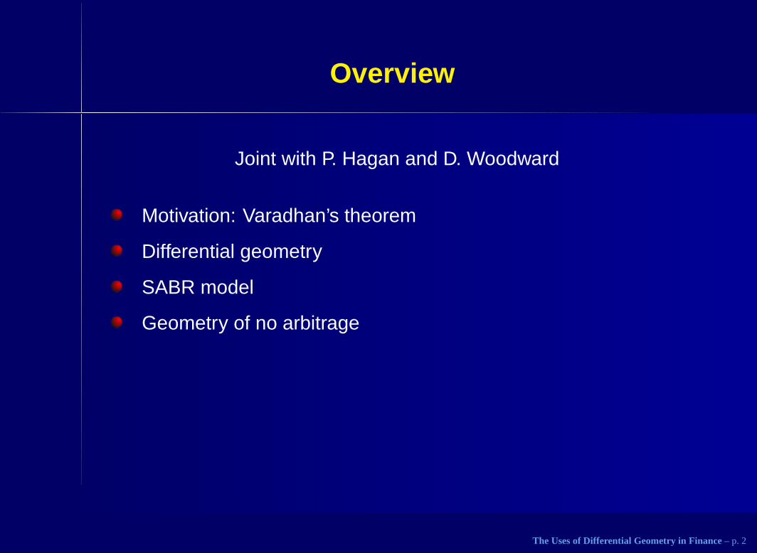
Joint with P. Hagan and D. Woodward
Motivation: Varadhan’s theorem
Differential geometry
SABR model
Geometry of no arbitrage
The Uses of Differential Geometry in Finance – p. 2

Varadhan’s theorem
This work has been motivated by the classical result of Varadhan.
It relates the short time asymptotic of the Green’s function of thebackward Kolmogorov equation to the differential geometry ofthe state space.
From the probabilistic point of view, the Green’s functionrepresents the transition probability of the diffusion, and it thuscarries all the information about the process.
Consequently, the geometry of the diffusion provides a naturalbook keeping device for calculations.
The Uses of Differential Geometry in Finance – p. 3

Varadhan’s theorem
Let W 1t , . . . ,W
dt be an N -dimensional Borwnian motion with
E[dW at dW
bt ] = ρabdt,
where ρ is a constant correlation matrix. We consider a driftless, timehomogeneous diffusion:
dXjt =
∑
a
σja(Xt)dW
at ,
defined in an open subset of RN (“state space”). Define the following
positive definite matrix:
gij (x) =∑
ab
ρabσia (x)σj
b (x) .
The Uses of Differential Geometry in Finance – p. 4
Varadhan’s theorem
Let GT,X(t, x) denote the transition probability (or Green’s function). Itsatisfies the following terminal value problem for the correspondingbackward Kolmogorov equation:
∂GT,X
∂t(t, x) +
1
2
∑
i,j
gij (x)∂GT,X
∂xi∂xj(t, x) = 0,
GT,X (T, x) = δ (x−X) .
Substitution t→ T − t transforms this into the initial value problem forthe heat equation:
∂GX
∂t(t, x) =
1
2
∑
i,j
gij (x)∂GX
∂xi∂xj(t, x) ,
GX (0, x) = δ (x−X) .
The Uses of Differential Geometry in Finance – p. 5
Varadhan’s theorem
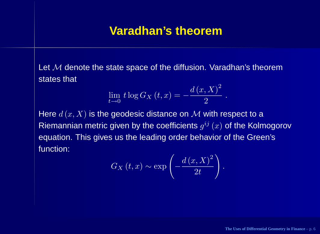
Let M denote the state space of the diffusion. Varadhan’s theoremstates that
limt→0
t logGX (t, x) = −d (x,X)2
2.
Here d (x,X) is the geodesic distance on M with respect to aRiemannian metric given by the coefficients gij (x) of the Kolmogorovequation. This gives us the leading order behavior of the Green’sfunction:
GX (t, x) ∼ exp
(
−d (x,X)2
2t
)
.
The Uses of Differential Geometry in Finance – p. 6
Varadhan’s theorem
To extract usable asymptotic information about the transitionprobability, more accurate analysis is necessary, but the choice of theRiemannian structure on M dictated by Varadhan’s theorem turns outto be key. Indeed, that Riemannian geometry becomes an importanttool in carrying out the calculations. Technically speaking, we are led tostudying the asymptotic properties of the perturbed Laplace - Beltramioperator on a Riemannian manifold. The relevant techniques go by thenames of the geometric optics or the WKB method.
The Uses of Differential Geometry in Finance – p. 7
Manifolds
A smooth manifold is a set M along with an open covering {Uα} andmaps hα : Uα → R
N such that all functions hβ ◦ h−1α : R
N → RN are
infinitely differentiable. The maps hα are called local coordinatesystems. Thus a manifold locally looks like the flat space. In thefollowing, all our manifolds will admit one global system of coordinates.
The Uses of Differential Geometry in Finance – p. 8

Tangent bundle
A tangent vector to a manifold M at a point x is a first order differentialoperator
V (x) =∑
i
Vi(x)∂
∂xi.
The vector space TxM of all tangent vectors at x is called the tangentspace at x, the union TM =
⋃
x TxM is called the tangent bundle.
The Uses of Differential Geometry in Finance – p. 9
Riemannian manifolds
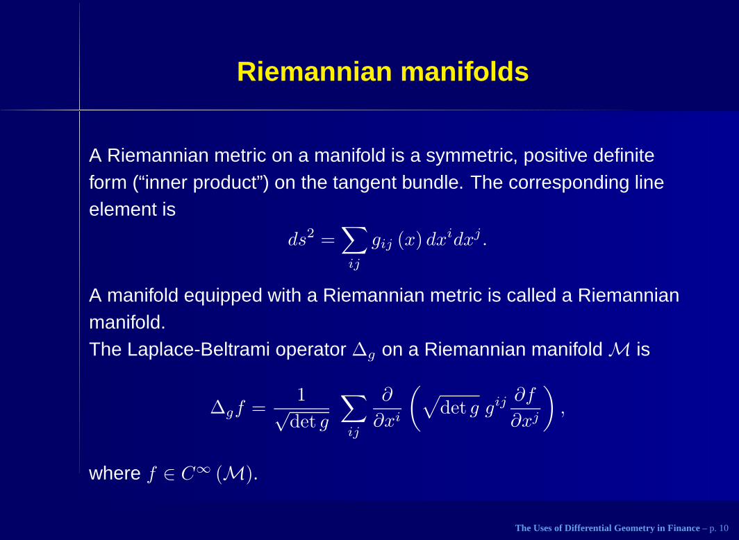
A Riemannian metric on a manifold is a symmetric, positive definiteform (“inner product”) on the tangent bundle. The corresponding lineelement is
ds2 =∑
ij
gij (x) dxidxj .
A manifold equipped with a Riemannian metric is called a Riemannianmanifold.The Laplace-Beltrami operator ∆g on a Riemannian manifold M is
∆gf =1√
det g
∑
ij
∂
∂xi
(
√
det g gij ∂f
∂xj
)
,
where f ∈ C∞ (M).
The Uses of Differential Geometry in Finance – p. 10
Example: Poincare geometry
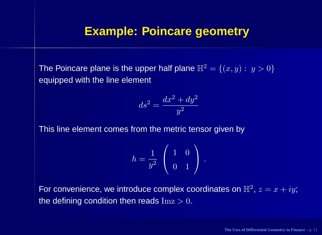
The Poincare plane is the upper half plane H2 = {(x, y) : y > 0}
equipped with the line element
ds2 =dx2 + dy2
y2
This line element comes from the metric tensor given by
h =1
y2
1 0
0 1
.
For convenience, we introduce complex coordinates on H2, z = x+ iy;
the defining condition then reads Imz > 0.
The Uses of Differential Geometry in Finance – p. 11
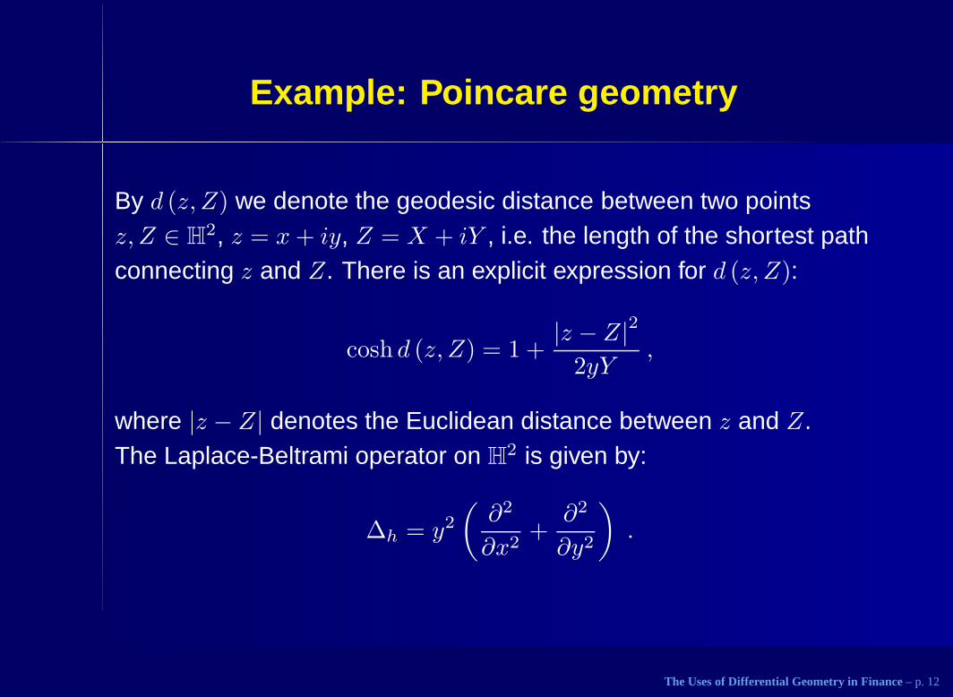
Example: Poincare geometry
By d (z, Z) we denote the geodesic distance between two pointsz, Z ∈ H
2, z = x+ iy, Z = X + iY , i.e. the length of the shortest pathconnecting z and Z. There is an explicit expression for d (z, Z):
cosh d (z, Z) = 1 +|z − Z|2
2yY,
where |z − Z| denotes the Euclidean distance between z and Z.The Laplace-Beltrami operator on H
2 is given by:
∆h = y2
(
∂2
∂x2+
∂2
∂y2
)
.
The Uses of Differential Geometry in Finance – p. 12
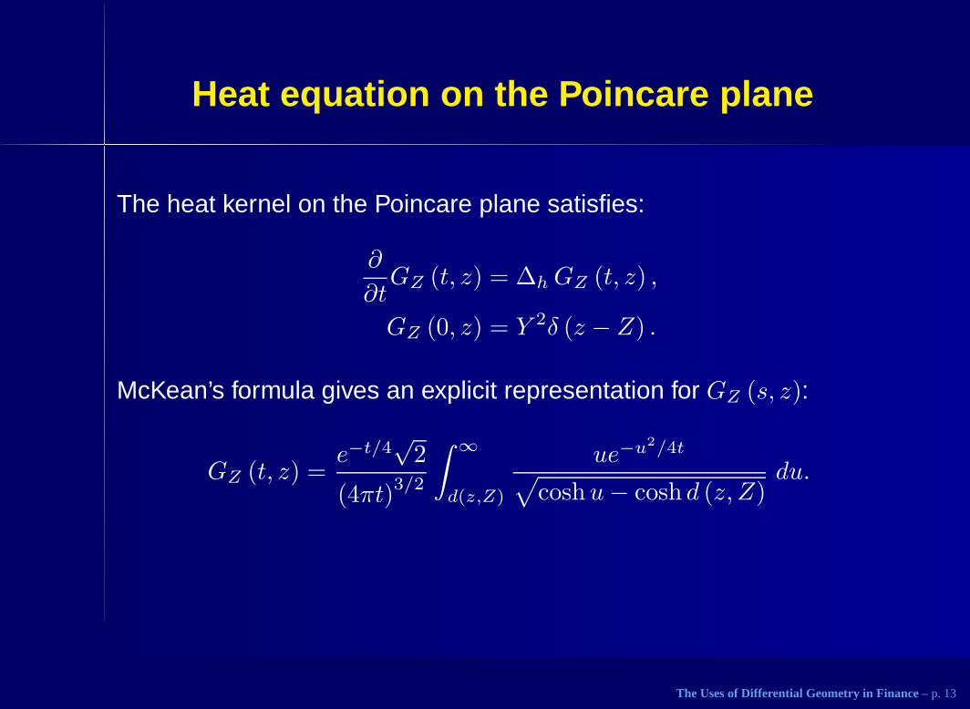
Heat equation on the Poincare plane
The heat kernel on the Poincare plane satisfies:
∂
∂tGZ (t, z) = ∆h GZ (t, z) ,
GZ (0, z) = Y 2δ (z − Z) .
McKean’s formula gives an explicit representation for GZ (s, z):
GZ (t, z) =e−t/4
√2
(4πt)3/2
∫ ∞
d(z,Z)
ue−u2/4t
√
coshu− cosh d (z, Z)du.
The Uses of Differential Geometry in Finance – p. 13
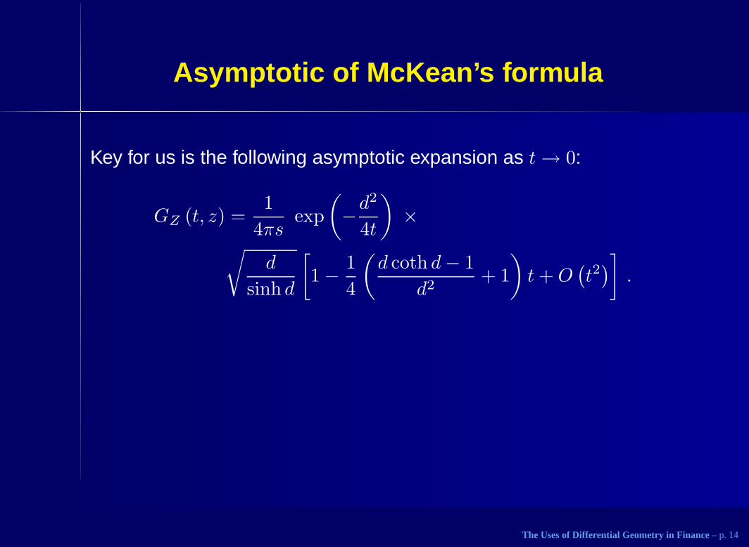
Asymptotic of McKean’s formula
Key for us is the following asymptotic expansion as t→ 0:
GZ (t, z) =1
4πsexp
(
−d2
4t
)
×√
d
sinh d
[
1 − 1
4
(
d coth d− 1
d2+ 1
)
t+O(
t2)
]
.
The Uses of Differential Geometry in Finance – p. 14
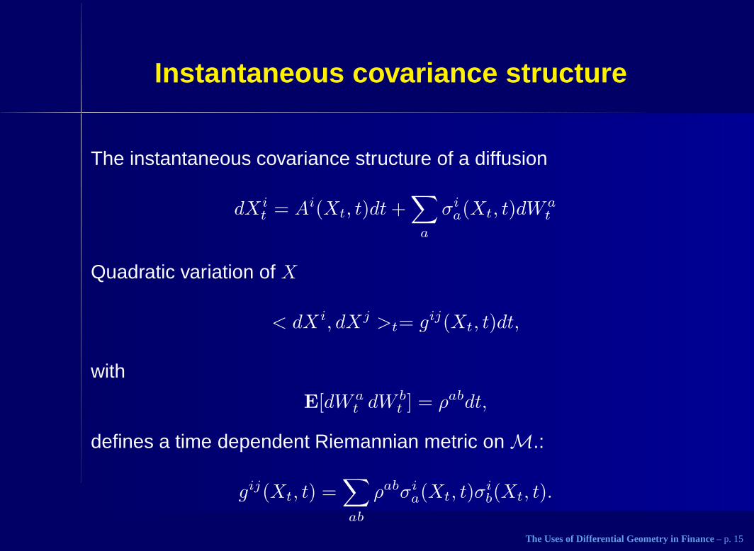
Instantaneous covariance structure
The instantaneous covariance structure of a diffusion
dXit = Ai(Xt, t)dt+
∑
a
σia(Xt, t)dW
at
Quadratic variation of X
< dXi, dXj >t= gij(Xt, t)dt,
with
E[dW at dW
bt ] = ρabdt,
defines a time dependent Riemannian metric on M.:
gij(Xt, t) =∑
ab
ρabσia(Xt, t)σ
ib(Xt, t).
The Uses of Differential Geometry in Finance – p. 15

SABR model
The dynamics of the forward rate Ft is
dFt = ΣtC(Ft)dWt,
dΣt = αΣtdZt.
Here Σt is the stochastic volatility parameter,
C(F ) = F β ,
and Wt and Zt are Brownian motions with
E [dWtdZt] = ρdt.
We supplement the dynamics with the initial condition F0 = f, Σ0 = σ.
The Uses of Differential Geometry in Finance – p. 16
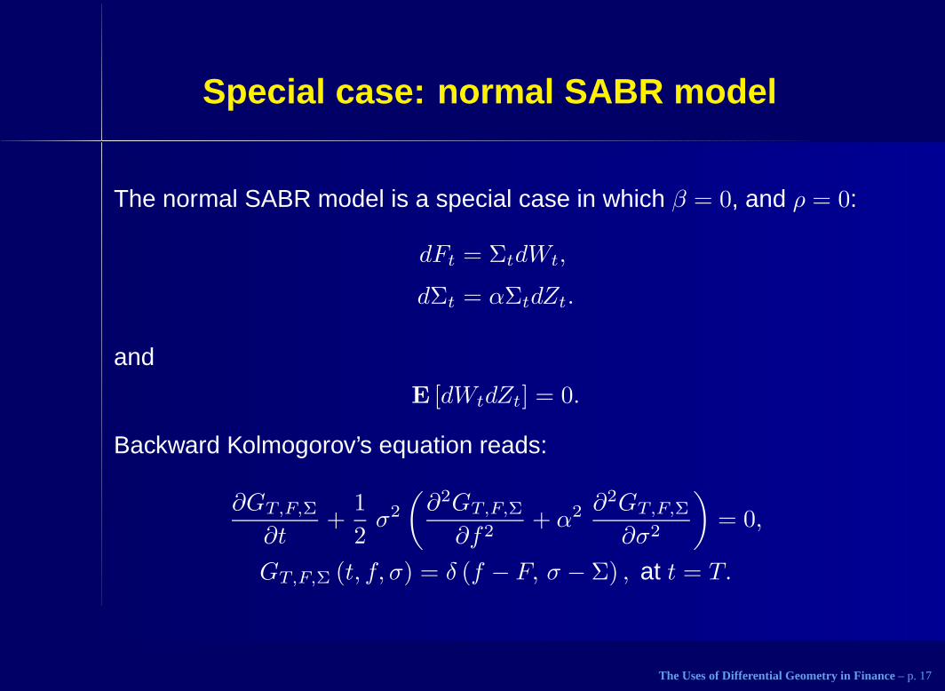
Special case: normal SABR model
The normal SABR model is a special case in which β = 0, and ρ = 0:
dFt = ΣtdWt,
dΣt = αΣtdZt.
and
E [dWtdZt] = 0.
Backward Kolmogorov’s equation reads:
∂GT,F,Σ
∂t+
1
2σ2
(
∂2GT,F,Σ
∂f2+ α2 ∂
2GT,F,Σ
∂σ2
)
= 0,
GT,F,Σ (t, f, σ) = δ (f − F, σ − Σ) , at t = T.
The Uses of Differential Geometry in Finance – p. 17

Special case: normal SABR model
After the transformation t→ T − t:
∂GF,Σ
∂t=
1
2σ2
(
∂2GT,F,Σ
∂f2+ α2 ∂
2GF,Σ
∂σ2
)
,
GF,Σ (0, f, σ) = δ (f − F, σ − Σ) .
This resembles the heat equation on the Poincare plane!
The Uses of Differential Geometry in Finance – p. 18
Normal SABR model and Poincare geometry
Brownian motion on the Poincare plane is described by:
dXt = YtdWt,
dYt = YtdZt,
with
E [dWtdZt] = 0.
This is the normal SABR model if we make the following identifications:
Xt = Fα2t,
Yt =1
αΣα2t .
The Uses of Differential Geometry in Finance – p. 19

Geometry of the full SABR model
The state space associated with the general SABR model has asomewhat more complicated geometry. Let S
2 denote the upper halfplane {(x, y) : y > 0} , equipped with the following metric g:
g =1
√
1 − ρ2 y2C (x)2
1 −ρC (x)
−ρC (x) C (x)2
.
This metric is a generalization of the Poincare metric: the case of ρ = 0
and C (x) = 1 reduces to the Poincare metric.
The Uses of Differential Geometry in Finance – p. 20

Geometry of the full SABR model
The metric g is the pullback of the Poincare metric under the followingdiffeomorphism. We choose p ≥ 0, and define a map φp : S
2 → H2 by
φp (z) =
(
1√
1 − ρ2
(∫ x
p
du
C (u)− ρy
)
, y
)
.
A consequence of this fact is that we have an explicit formula for thegeodesic distance δ (z, Z) on S
2:
cosh δ (z, Z) = cosh d (φp (z) , φp (Z))
= 1 +
(
∫ x
Xdu
C(u)
)2
− 2ρ (y − Y )∫ x
Xdu
C(u) + (y − Y )2
2 (1 − ρ2) yY.
The Uses of Differential Geometry in Finance – p. 21
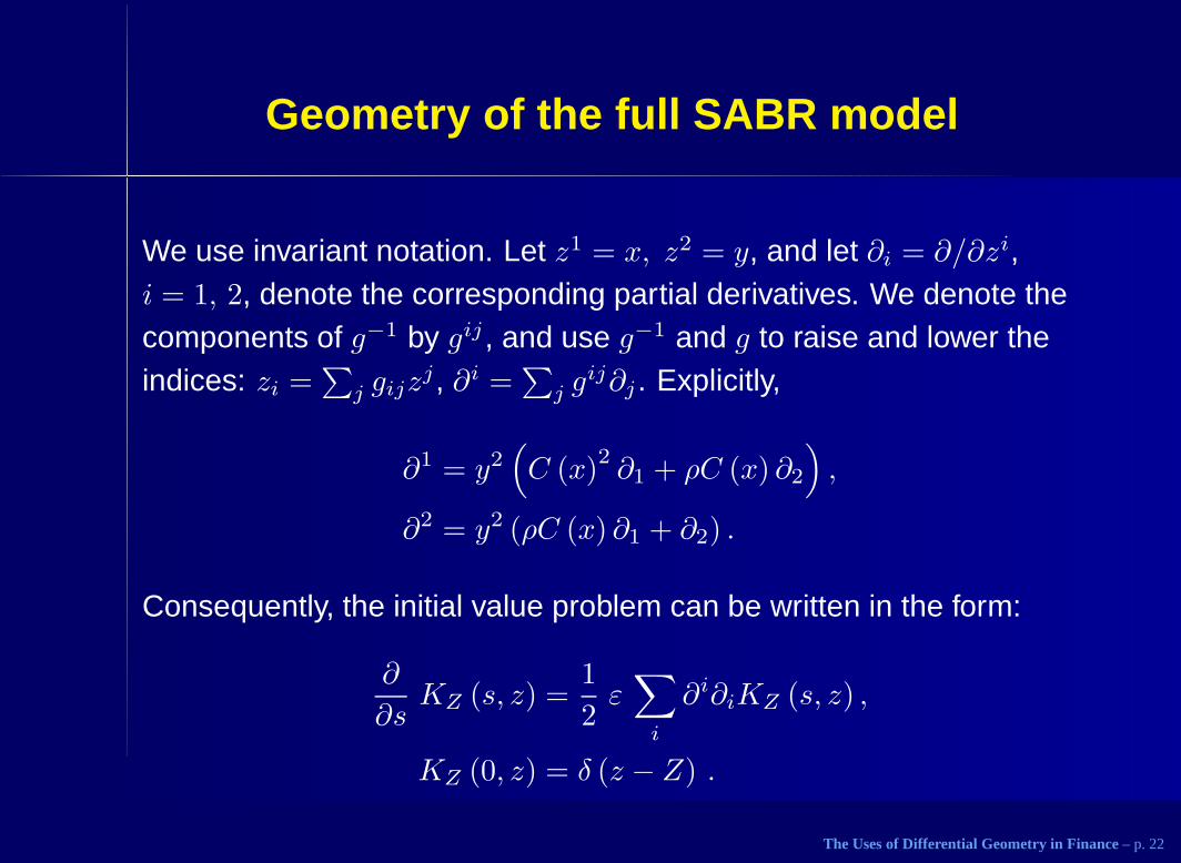
Geometry of the full SABR model
We use invariant notation. Let z1 = x, z2 = y, and let ∂i = ∂/∂zi,i = 1, 2, denote the corresponding partial derivatives. We denote thecomponents of g−1 by gij , and use g−1 and g to raise and lower theindices: zi =
∑
j gijzj , ∂i =
∑
j gij∂j . Explicitly,
∂1 = y2(
C (x)2∂1 + ρC (x) ∂2
)
,
∂2 = y2 (ρC (x) ∂1 + ∂2) .
Consequently, the initial value problem can be written in the form:
∂
∂sKZ (s, z) =
1
2ε∑
i
∂i∂iKZ (s, z) ,
KZ (0, z) = δ (z − Z) .
The Uses of Differential Geometry in Finance – p. 22
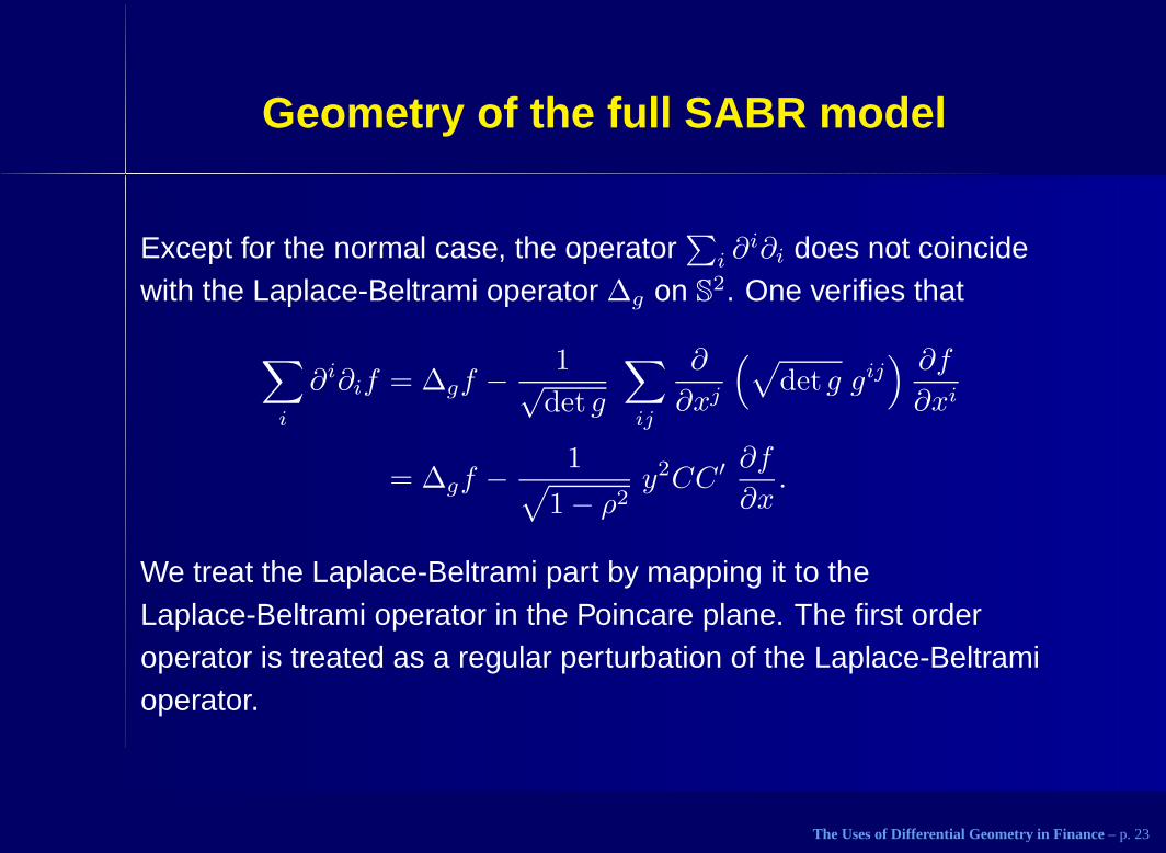
Geometry of the full SABR model
Except for the normal case, the operator∑
i ∂i∂i does not coincide
with the Laplace-Beltrami operator ∆g on S2. One verifies that
∑
i
∂i∂if = ∆gf − 1√det g
∑
ij
∂
∂xj
(
√
det g gij) ∂f
∂xi
= ∆gf − 1√
1 − ρ2y2CC′ ∂f
∂x.
We treat the Laplace-Beltrami part by mapping it to theLaplace-Beltrami operator in the Poincare plane. The first orderoperator is treated as a regular perturbation of the Laplace-Beltramioperator.
The Uses of Differential Geometry in Finance – p. 23
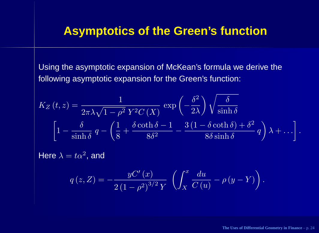
Asymptotics of the Green’s function
Using the asymptotic expansion of McKean’s formula we derive thefollowing asymptotic expansion for the Green’s function:
KZ (t, z) =1
2πλ√
1 − ρ2 Y 2C (X)exp
(
− δ2
2λ
)
√
δ
sinh δ[
1 − δ
sinh δq −
(
1
8+δ coth δ − 1
8δ2− 3 (1 − δ coth δ) + δ2
8δ sinh δq
)
λ+ . . .
]
.
Here λ = tα2, and
q (z, Z) = − yC ′ (x)
2 (1 − ρ2)3/2
Y
(∫ x
X
du
C (u)− ρ (y − Y )
)
.
The Uses of Differential Geometry in Finance – p. 24

Probability distribution in the SABR model
STEP 1. We integrate the asymptotic joint density over the terminalvolatility variable Y to find the marginal density for the forward x:
PX (t, x, y) =
∫ ∞
0
KZ (t, z) dY
=1
2πλ√
1 − ρ2 C (X)
∫ ∞
0
e−δ2/2λ
√
δ
sinh δ
[
1 − δ
sinh δq
−1
8λ
(
1 +δ coth δ − 1
δ2− 3 (1 − δ coth δ) + δ2
δ sinh δq
)]
dY
Y 2.
Here again, δ (z, Z) denotes the geodesic distance on S2.
The Uses of Differential Geometry in Finance – p. 25
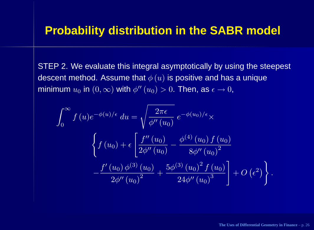
Probability distribution in the SABR model
STEP 2. We evaluate this integral asymptotically by using the steepestdescent method. Assume that φ (u) is positive and has a uniqueminimum u0 in (0,∞) with φ′′ (u0) > 0. Then, as ǫ→ 0,
∫ ∞
0
f (u)e−φ(u)/ǫ du =
√
2πǫ
φ′′ (u0)e−φ(u0)/ǫ×
{
f (u0) + ǫ
[
f ′′ (u0)
2φ′′ (u0)− φ(4) (u0) f (u0)
8φ′′ (u0)2
−f′ (u0)φ
(3) (u0)
2φ′′ (u0)2 +
5φ(3) (u0)2f (u0)
24φ′′ (u0)3
]
+O(
ǫ2)
}
.
The Uses of Differential Geometry in Finance – p. 26

Probability distribution in the SABR model
STEP 3. The exponent:
φ (Y ) =1
2δ (z, Z)
2,
has a unique minimum at Y0 given by
Y0 = y√
ζ2 − 2ρζ + 1 ,
where
ζ =1
y
∫ x
X
du
C (u).
Y0 is the “most likely value” of Y , and thus Y0C (X) (when expressed inthe original units) is the leading contribution to the observed impliedvolatility.
The Uses of Differential Geometry in Finance – p. 27

Probability distribution in the SABR model
STEP 4. Let D (ζ) denote the value of δ (z, Z) with Y = Y0. Explicitly,
D (ζ) = log
√
ζ2 − 2ρζ + 1 + ζ − ρ
1 − ρ.
We also introduce the notation:
I (ζ) =√
ζ2 − 2ρζ + 1
= coshD (ζ) − ρ sinhD (ζ) .
The Uses of Differential Geometry in Finance – p. 28
Probability distribution in the SABR model
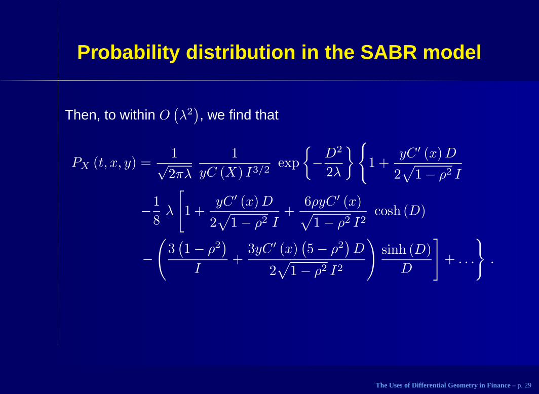
Then, to within O(
λ2)
, we find that
PX (t, x, y) =1√2πλ
1
yC (X) I3/2exp
{
−D2
2λ
}
{
1 +yC ′ (x)D
2√
1 − ρ2 I
−1
8λ
[
1 +yC ′ (x)D
2√
1 − ρ2 I+
6ρyC ′ (x)√
1 − ρ2 I2cosh (D)
−(
3(
1 − ρ2)
I+
3yC ′ (x)(
5 − ρ2)
D
2√
1 − ρ2 I2
)
sinh (D)
D
]
+ . . .
}
.
The Uses of Differential Geometry in Finance – p. 29
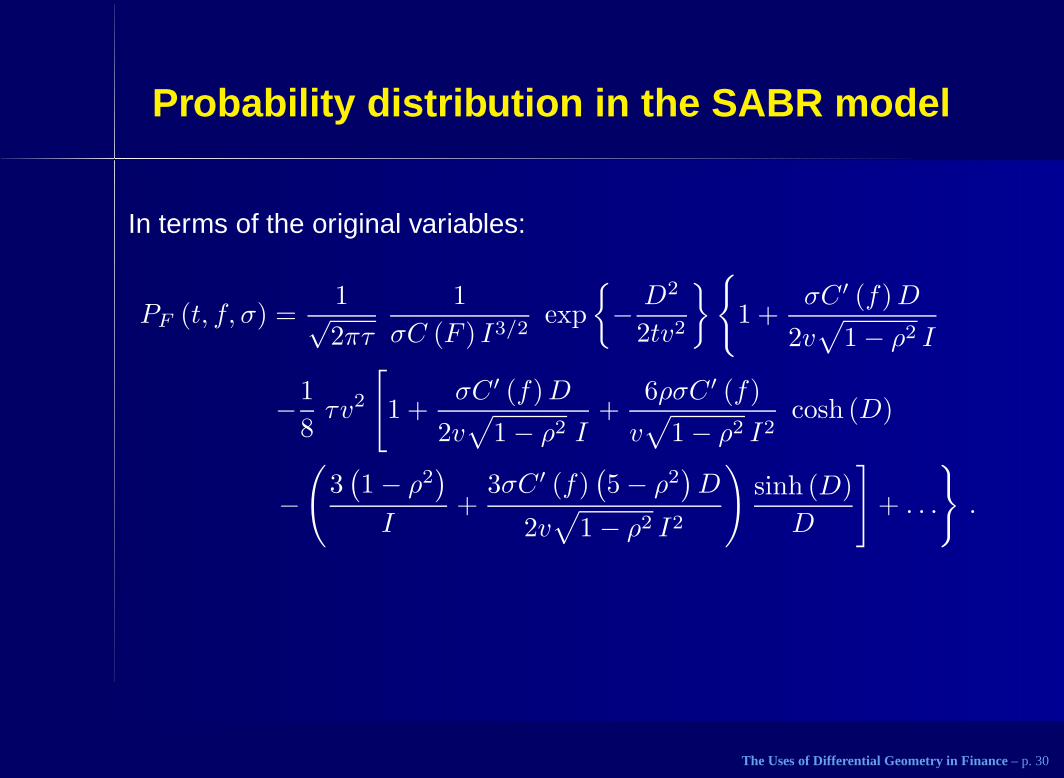
Probability distribution in the SABR model
In terms of the original variables:
PF (t, f, σ) =1√2πτ
1
σC (F ) I3/2exp
{
− D2
2tv2
}
{
1 +σC ′ (f)D
2v√
1 − ρ2 I
−1
8τv2
[
1 +σC ′ (f)D
2v√
1 − ρ2 I+
6ρσC ′ (f)
v√
1 − ρ2 I2cosh (D)
−(
3(
1 − ρ2)
I+
3σC ′ (f)(
5 − ρ2)
D
2v√
1 − ρ2 I2
)
sinh (D)
D
]
+ . . .
}
.
The Uses of Differential Geometry in Finance – p. 30

Line bundles over manifolds
A line bundle over a manifold M is a manifold L together with a mapπ : L → M such that:
Each fiber π−1(x) is isomorphic to R.
Each x ∈ M has a neighborhood U ⊂ M and a diffeomorphismπ−1(U) ≃ U × R.
The simplest example of a line bundle is the trivial line bundle,L = M× R. A general line bundle looks locally like a trivial line bundle.A smooth map φ : M → L is called a section of L if π ◦ φ = Identity.The set of all sections is denoted by Γ(L).
The Uses of Differential Geometry in Finance – p. 31

Connections on line bundles
A connection ∇ on a line bundle L → M is a way to calculatederivatives of sections of L along tangent vectors.
For a, b ∈ R, and φ, ψ ∈ Γ(L),
∇(aφ+ bψ) = a∇φ+ b∇ψ.
For f ∈ C∞(M), and φ ∈ Γ (L),
∇(fφ) = df ⊗ φ+ f∇φ.
For example, on a trivial bundle L = M× R, all connections are of theform ∇ = d+ ω, where ω is a 1-form on M.
The Uses of Differential Geometry in Finance – p. 32
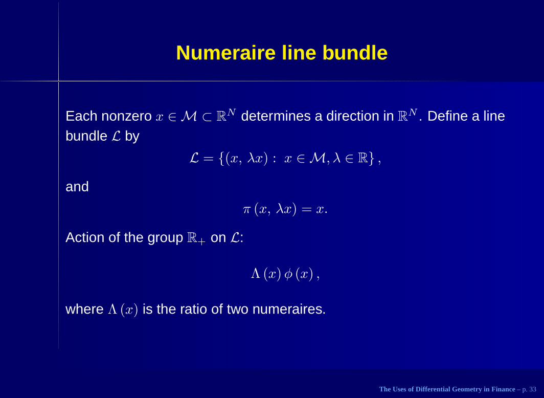
Numeraire line bundle
Each nonzero x ∈ M ⊂ RN determines a direction in R
N . Define a linebundle L by
L = {(x, λx) : x ∈ M, λ ∈ R} ,
and
π (x, λx) = x.
Action of the group R+ on L:
Λ (x)φ (x) ,
where Λ (x) is the ratio of two numeraires.
The Uses of Differential Geometry in Finance – p. 33
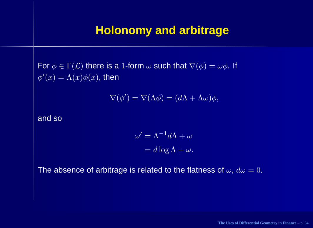
Holonomy and arbitrage
For φ ∈ Γ(L) there is a 1-form ω such that ∇(φ) = ωφ. Ifφ′(x) = Λ(x)φ(x), then
∇(φ′) = ∇(Λφ) = (dΛ + Λω)φ,
and so
ω′ = Λ−1dΛ + ω
= d log Λ + ω.
The absence of arbitrage is related to the flatness of ω, dω = 0.
The Uses of Differential Geometry in Finance – p. 34
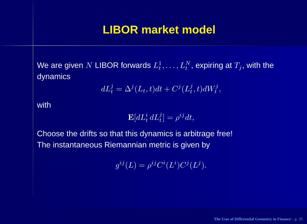
LIBOR market model
We are given N LIBOR forwards L1t , . . . , L
Nt , expiring at Tj , with the
dynamics
dLjt = ∆j(Lt, t)dt+ Cj(Lj
t , t)dWjt ,
with
E[dLit dL
jt ] = ρijdt,
Choose the drifts so that this dynamics is arbitrage free!The instantaneous Riemannian metric is given by
gij(L) = ρijCi(Li)Cj(Lj).
The Uses of Differential Geometry in Finance – p. 35

LIBOR market model
We let Pj(L) denote the price of the zero coupon bond expiring at Tj ,
Pj(L) =∏
1≤i≤j
1
1 + δiLi,
where δi is the day count fraction. Therefore, if
Λ(L) =Pk(L)
Pj(L),
the corresponding connection forms differ by
d log
∏
j+1≤i≤k
1
1 + δiLi
.
The Uses of Differential Geometry in Finance – p. 36

LIBOR market model
Therefore,
ωi =
− δi1 + δiLi
t
, if j + 1 ≤ i ≤ k,
δi1 + δiLi
t
, if k + 1 ≤ i ≤ j,
0, otherwise.
and thus
∆j =∑
i
gjiωi
= Cj∑
i
ρjiCiωi.
The Uses of Differential Geometry in Finance – p. 37
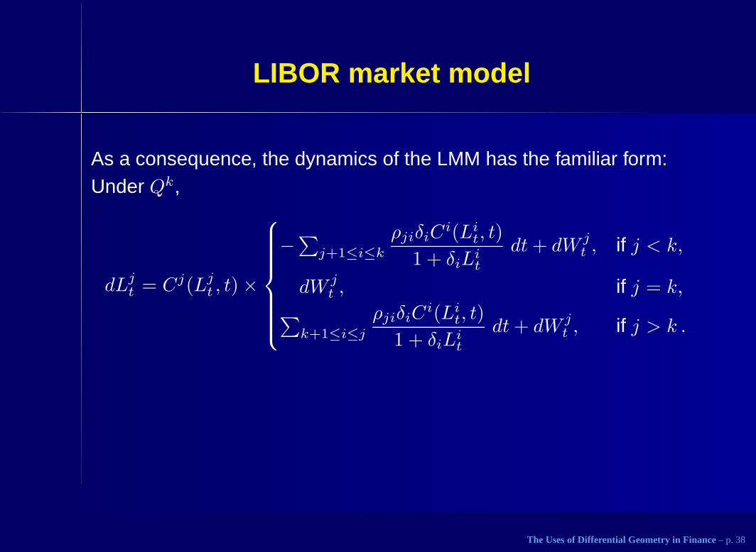
LIBOR market model
As a consequence, the dynamics of the LMM has the familiar form:Under Qk,
dLjt = Cj(Lj
t , t) ×
−∑
j+1≤i≤k
ρjiδiCi(Li
t, t)
1 + δiLit
dt+ dW jt , if j < k,
dW jt , if j = k,
∑
k+1≤i≤j
ρjiδiCi(Li
t, t)
1 + δiLit
dt+ dW jt , if j > k .
The Uses of Differential Geometry in Finance – p. 38
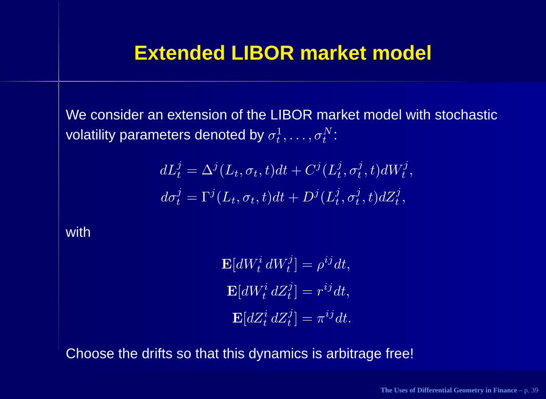
Extended LIBOR market model
We consider an extension of the LIBOR market model with stochasticvolatility parameters denoted by σ1
t , . . . , σNt :
dLjt = ∆j(Lt, σt, t)dt+ Cj(Lj
t , σjt , t)dW
jt ,
dσjt = Γj(Lt, σt, t)dt+Dj(Lj
t , σjt , t)dZ
jt ,
with
E[dW it dW
jt ] = ρijdt,
E[dW it dZ
jt ] = rijdt,
E[dZit dZ
jt ] = πijdt.
Choose the drifts so that this dynamics is arbitrage free!
The Uses of Differential Geometry in Finance – p. 39

Extended LIBOR market model
The state space of this model has dimension 2N and theinstantaneous Riemannian metric is given by:
gij(L, σ) =
ρijCi(Li, σi)Cj(Lj , σj), if 1 ≤ i, j ≤ N,
πijCi(Li, σi)Dj(Lj , σj), if 1 ≤ i ≤ N, N + 1 ≤ j ≤ 2N,
πijDi(Li, σi)Cj(Lj , σj), if N + 1 ≤ i ≤ 2N, 1 ≤ j ≤ N,
rijDi(Li, σi)Dj(Lj , σj), if N + 1 ≤ i, j ≤ 2N.
Calculation of the connection form ω is identical to that of the LIBORmodel.
The Uses of Differential Geometry in Finance – p. 40
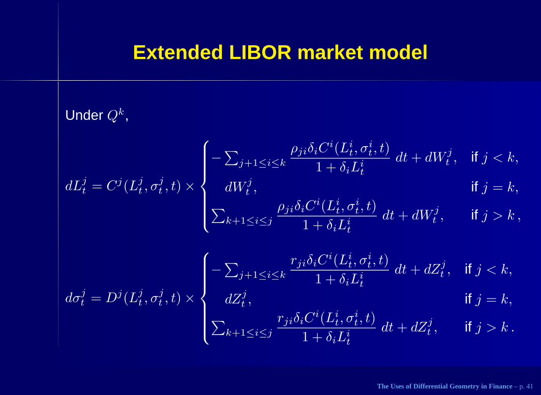
Extended LIBOR market model
Under Qk,
dLjt = Cj(Lj
t , σjt , t) ×
−∑j+1≤i≤k
ρjiδiCi(Li
t, σit, t)
1 + δiLit
dt+ dW jt , if j < k,
dW jt , if j = k,
∑
k+1≤i≤j
ρjiδiCi(Li
t, σit, t)
1 + δiLit
dt+ dW jt , if j > k ,
dσjt = Dj(Lj
t , σjt , t) ×
−∑j+1≤i≤k
rjiδiCi(Li
t, σit, t)
1 + δiLit
dt+ dZjt , if j < k,
dZjt , if j = k,
∑
k+1≤i≤j
rjiδiCi(Li
t, σit, t)
1 + δiLit
dt+ dZjt , if j > k .
The Uses of Differential Geometry in Finance – p. 41