the use of topographic-isostatic mass information in ...hss.ulb.uni-bonn.de/2007/1024/1024.pdf ·...
TRANSCRIPT

Institut für Geodäsie und Geoinformation der Universität BonnAstronomische, Physikalische und Mathematische Geodäsie
The Use of Topographic-Isostatic Mass Informationin Geodetic Applications
Inaugural–Dissertation zur
Erlangung des akademischen Grades
Doktor–Ingenieur (Dr.–Ing.)
der Hohen Landwirtschaftlichen Fakultät
der Rheinischen Friedrich–Wilhelms–Universität
zu Bonn
vorgelegt am 5. Februar 2007 von
M.Sc. Atef Abd–Elhakeem Makhloofaus El Minia, Ägypten
D 98

Referent: Prof. Dr.–Ing. K. H. Ilk
Korreferent: Prof. Dr.–Ing. B. Witte
Tag der mündlichen Prüfung: 13.04.2007
Gedruckt bei: Diese Dissertation ist auf dem Hochschulschriften-
server der ULB Bonn
http://hss.ulb.uni-bonn.de/diss_online
elektronisch publiziert.

Zusammenfassung
Die Gravitationsfeldeffekte der topographisch-isostatischen Massen stellen eine wichtige Information deshochfrequenten Anteils des Gravitationsfeldes dar. In dieser Arbeit werden die physikalisch-mathematischenGrundlagen der klassischen topographisch-isostatischen Modelle dargestellt. Es werden die verschiedenenisostatischen Modelle mathematisch formuliert, wobei auf der Modellbildungsseite der Schwerpunkt auf dersphärischen Approximation liegt und von den Anwendungen die Beobachtungstypen der Flugzeuggravimetrieund der modernen Satellitenmethoden im Vordergrund stehen. Neben der Darstellung der topographisch-isostatischen Masseneffekte durch sphärische Volumenintegrale, diskretisiert durch sphärische Volumenele-mente, werden die Reihendarstellungen nach Kugelflächenfunktionen und nach ortslokalisierenden Basis-funktionen zugrunde gelegt. Detaillierte Formeln werden für den direkten bzw. den sekundären indirektentopographischen Effekt in den Schwerewerten und den primären indirekten Effekt in den Geoidhöhen für dieverschiedenen Darstellungen angegeben. Schliesslich werden Formeln für die Berechnung der Fernzoneneffekteder topographisch-isostatischen Massen angegeben. Hierzu wird eine von Molodenskii angegebene Methodeangewendet, die auf der Kugelfunktionsentwicklung der topographisch-isostatischen Massen beruht. Um-fangreiche Rechenbeispiele vermitteln einen Eindruck von der Grösse und der Verteilung der verschiedenenEffekte, basierend auf unterschiedlich aufgelösten regionalen und globalen Testgebieten.
Summary
The gravity field effects of the topographic-isostatic masses represent an important information of the high-frequent part of the gravity field. In this work the physical-mathematical basics of the classical topographic-isostatic models are presented. These models are formulated mathematically with the emphasis on a sphericalapproximation from the modelling point of view and on the observables of airborne gravimetry but also of themodern satellite techniques from the application point of view. Besides the representation of the topographic-isostatic mass effects by volume integrals, discretized by spherical volume elements, the representationsby series of spherical harmonics and space localizing base functions are considered. Detailed formulae arepresented for the direct and secondary indirect topographical effect as well as for the primary indirecttopographical effect in the geoid heights for the different representations. Finally, extended test computationsgive an impression of the size and distribution of the various effects for regional and global test areas withdifferent resolutions of the topography.
4
Table of Contents
1 Introduction 7
2 Topographic masses and the gravity field of the Earth 10
2.1 The gravity potential and its derivatives . . . . . . . . . . . . . . . . . . . . . . . . . . . . . . 10
2.1.1 Newton’s law of gravitation . . . . . . . . . . . . . . . . . . . . . . . . . . . . . . . . . 10
2.1.2 The gravitational field of a solid body . . . . . . . . . . . . . . . . . . . . . . . . . . . 11
2.1.3 The potential of the topographical and compensating masses . . . . . . . . . . . . . . 13
2.1.4 The gravitational field of a single mass layer . . . . . . . . . . . . . . . . . . . . . . . . 14
2.2 The geodetic boundary value problems . . . . . . . . . . . . . . . . . . . . . . . . . . . . . . . 16
2.2.1 Gravitational field and gravity field . . . . . . . . . . . . . . . . . . . . . . . . . . . . . 16
2.2.2 Normal figure and normal field . . . . . . . . . . . . . . . . . . . . . . . . . . . . . . . 17
2.2.3 The boundary value problem of Stokes . . . . . . . . . . . . . . . . . . . . . . . . . . . 18
2.2.4 Topographic isostatic effects in Stokes’ boundary value problem . . . . . . . . . . . . . 20
2.2.5 The role of topography in Molodenskii’s boundary value problem . . . . . . . . . . . . 22
2.3 Topographic-isostatic effects in airborne gravimetry . . . . . . . . . . . . . . . . . . . . . . . . 26
2.4 Topographic-isostatic mass effects in satellite application . . . . . . . . . . . . . . . . . . . . . 28
2.4.1 Improperly posed problems in satellite geodesy . . . . . . . . . . . . . . . . . . . . . . 28
2.4.2 The use of topographic-isostatic mass effects in the Satellite -to- Satellite Trackingtechnique . . . . . . . . . . . . . . . . . . . . . . . . . . . . . . . . . . . . . . . . . . . 29
2.4.3 The use of topographic-isostatic mass effects in Satellite Gravity Gradiometry . . . . 30
3 Mass models of the Earth’s topography 32
3.1 Digital terrain model . . . . . . . . . . . . . . . . . . . . . . . . . . . . . . . . . . . . . . . . . 32
3.2 Digital density models . . . . . . . . . . . . . . . . . . . . . . . . . . . . . . . . . . . . . . . . 33
3.3 Isostatic models . . . . . . . . . . . . . . . . . . . . . . . . . . . . . . . . . . . . . . . . . . . . 33
3.3.1 Airy-Heiskanen model . . . . . . . . . . . . . . . . . . . . . . . . . . . . . . . . . . . . 34
3.3.2 Pratt-Hayford model . . . . . . . . . . . . . . . . . . . . . . . . . . . . . . . . . . . . . 39
3.3.3 Combined Airy-Pratt model . . . . . . . . . . . . . . . . . . . . . . . . . . . . . . . . . 43
3.3.4 Vening-Meinesz model . . . . . . . . . . . . . . . . . . . . . . . . . . . . . . . . . . . . 43
3.4 Helmert’s models of condensation . . . . . . . . . . . . . . . . . . . . . . . . . . . . . . . . . . 46

Table of Contents 5
4 Computation of the gravitational effects of the topographic-isostatic masses 48
4.1 Direct integration method . . . . . . . . . . . . . . . . . . . . . . . . . . . . . . . . . . . . . . 48
4.1.1 Gravitational potential and its derivatives modelled by prisms . . . . . . . . . . . . . 49
4.1.2 Gravitational potential and its derivatives modelled by tesseroids (using the analyticvertical integration) . . . . . . . . . . . . . . . . . . . . . . . . . . . . . . . . . . . . . 54
4.2 Spherical harmonic expansion . . . . . . . . . . . . . . . . . . . . . . . . . . . . . . . . . . . . 66
4.2.1 Effects of topographic-isostatic masses in satellite applications . . . . . . . . . . . . . 66
4.2.2 Spherical harmonic expansion for calculating the far-zone topographical effects . . . . 76
4.3 Space localizing base functions . . . . . . . . . . . . . . . . . . . . . . . . . . . . . . . . . . . 87
4.3.1 Direct topographical effects on gravity . . . . . . . . . . . . . . . . . . . . . . . . . . . 87
4.3.2 Primary indirect topographical effect . . . . . . . . . . . . . . . . . . . . . . . . . . . . 89
5 Numerical analysis 91
5.1 Test regions . . . . . . . . . . . . . . . . . . . . . . . . . . . . . . . . . . . . . . . . . . . . . . 91
5.1.1 Canadian Rocky Mountains . . . . . . . . . . . . . . . . . . . . . . . . . . . . . . . . . 91
5.1.2 Himalaya . . . . . . . . . . . . . . . . . . . . . . . . . . . . . . . . . . . . . . . . . . . 91
5.1.3 Asia . . . . . . . . . . . . . . . . . . . . . . . . . . . . . . . . . . . . . . . . . . . . . . 91
5.1.4 Earth . . . . . . . . . . . . . . . . . . . . . . . . . . . . . . . . . . . . . . . . . . . . . 93
5.2 Computation aspects . . . . . . . . . . . . . . . . . . . . . . . . . . . . . . . . . . . . . . . . . 93
5.2.1 Discretization effects . . . . . . . . . . . . . . . . . . . . . . . . . . . . . . . . . . . . . 93
5.2.2 Surface spherical harmonic expansion of the topography . . . . . . . . . . . . . . . . . 96
5.2.3 Near-zone and far-zone aspects . . . . . . . . . . . . . . . . . . . . . . . . . . . . . . . 102
5.3 Effects of topographic-isostatic masses at the surface of the Earth and at aeroplane altitudes 103
5.3.1 Near-zone topography effects . . . . . . . . . . . . . . . . . . . . . . . . . . . . . . . . 103
5.3.2 Far-zone topography effects . . . . . . . . . . . . . . . . . . . . . . . . . . . . . . . . . 108
5.4 Effect of topographic-isostatic masses in satellite applications . . . . . . . . . . . . . . . . . . 119
5.4.1 Topographic-isostatic effects on gravity gradients . . . . . . . . . . . . . . . . . . . . . 119
5.4.2 Topographic-isostatic effects on SST observations . . . . . . . . . . . . . . . . . . . . . 132
6 Discussion and conclusions 135
References 138
A Appendix 146
A.1 Truncation coefficients for the direct terrain effect . . . . . . . . . . . . . . . . . . . . . . . . 146
A.1.1 Helmert’s second method of condensation . . . . . . . . . . . . . . . . . . . . . . . . . 146
A.1.2 Helmert’s first or generalized method of condensation . . . . . . . . . . . . . . . . . . 150
A.1.3 Airy-Heiskanen model . . . . . . . . . . . . . . . . . . . . . . . . . . . . . . . . . . . . 151
List of Figures 152
List of Tables 155


7
1. Introduction
The topographic masses represent an important source of gravity field information especially in the high-frequency band of the gravity field spectrum, even if the detailed density function inside the topographicmasses is only approximately known. The gravity field effect of the visible topography is partially reducedby isostatic compensation mechanisms – the net effect of both are nevertheless significant larger and of morepronounced high-frequent character than the effects of the inhomogeneities inside the crust of the Earth.With the global detailed digital elevation models of the topography at the continents and of the bathymetryat the oceans, accessible nowadays, a very important source of gravity field information is available. In thisresearch, only geodetically relevant aspects are treated, but many of the topics discussed in this work areimportant also in structural and exploration geophysics or in geological applications.
In geodesy, the topographic-isostatic masses can be used in a threefold way: (1) the solution of the Laplaceequation within the frame of the geodetic boundary value problem of Stokes requires a mass-free space outsidethe boundary surface, the (co-)geoid. This is the reason that the topographic masses have to be removedor shifted inside the geoid; the effects of this process have to be restored after the solution to reconstitutethe original situation. But also in case of the geodetic boundary value problem according to Molodenskii thenumerical results can be achieved in a simpler and more accurate way by making use of the topographicinformation than without it. (2) A rough topography causes strong oscillations in the gravity field functionals,e.g., gravity anomalies and disturbances, deflections of the vertical or the second derivatives of the gravitypotential. If these functionals can be filtered by the topographic-isostatic masses then the filtered functionalscan be interpolated or extrapolated much easier and more precise than by using the unfiltered quantities.Because of the fact that the various geodetic applications of gravity require the knowledge of the gravityfield functionals at locations different from the measurement locations the prediction is a frequently appliedprocedure. These principle ideas are behind the so-called remove-restore procedure, where the observationalfunctionals of the gravity field are reduced by the known global gravity field information, based on preciseglobal gravity field models and the high frequent effects of the topographic-isostatic masses. The resultingresidual gravity field functionals are considerably smoother than before and can be represented by generalizedapproximation/prediction techniques such as Least Squares Collocation. (3) The determination of the gravityfield from observations at a certain altitude above sea level, especially at aircraft or satellite altitudes, is animproperly posed problem in the sense that small changes in the observations at flight level produce largeeffects in the gravity field parameters on the Earth’s surface or geoid level. This holds especially for thehigh-frequency constituents of the observation spectrum. To prevent the results from unrealistic oscillationsin the parameters, regularization techniques are usually applied in very poorly conditioned cases. Most ofthe regularization methods represent a filtering procedure and the filtering property can be controlled by aregularization parameter. This is critical in those cases where the signal shows similar spectral characteristicsas the observation noise. The topographic-isostatic masses represent a gravity field information, especially inthe high frequency band of the gravity field spectrum, which can be superposed with the measurement noisein aircraft or satellite altitude. Therefore, it is helpful, if those signal parts are reduced before the downwardcontinuation and restored afterwards. In this case, it can be assumed that the high-frequency part in theobservations is mainly caused by the observation noise, which can be filtered without loosing gravity fieldinformation.
Because of the local effects of the topographic masses in the gravity field functionals the planar approxima-tion was frequently applied in the past. In global applications, this approximation cannot be used anymore(see Novák el al. 2001). Therefore, the very efficient fast Fourier transformation (FFT) techniques will notbe applied for large-scale computations as demonstrated by Schwarz et al. (1990) in case of applicationsin airborne gravimetry in this investigation. This holds especially for large-scale regional or even globalapplications in case of the processing of observables of the new gravity satellite missions. There are two prin-cipal possibilities for calculating the effects of the topographic-isostatic masses on gravitational functionalsin spherical approximation: the representation of the topographic masses by any spherical discretisation inform of spherical compartments (e.g. defined by spherical coordinate lines) and a subsequent integration(Abd-Elmotaal 1995b, Smith et al. 2001; Tenzer et al. 2003; Heck 2003) or the representation of Newton’s

8 1. Introduction
integral by a spherical harmonic expansion (e.g., Sünkel 1985; Rummel et al. 1988; Tsoulis 1999a, 2001).Sjöberg (1998a) implemented the formulae for the exterior Airy-Heiskanen topographic-isostatic gravity po-tential and the corresponding gravity anomalies. Surface spherical harmonics are base functions with globalsupport and they are tailored to global computations. This is the reason that usually the gravity potential ismodelled by a spherical harmonic expansion. Nevertheless, the heterogeneity of the gravity field cannot beproperly taken into account with the help of spherical harmonics as base functions with global support. Themaximum degree must be adapted to the roughest gravity field features which are concentrated especiallyin the regions with very high mountains. In most of the regions the maximum degree could be much smal-ler. The representation of gravity field functionals by spherical harmonics is very efficient but limited to anupper spherical harmonic degree of about 2700 which corresponds to a 4 arc-minute resolution. Beyond thisdegree numerical computation problems concerning the stability of the recursive computation of Legendre’spolynomials occur (see, e.g., Holmes and Featherstone 2002) and increasing of the computational time. It ispreferable to model the gravity field only up to a moderate spherical harmonic degree to represent properlymost of the regions of the Earth; the specific detailed features tailored to the individual gravity field charac-teristics in areas of rough gravity field signal can be modelled additionally by space localizing base functionssuch as spherical spline functions (Freeden et al. 1998) or spherical wavelets (Freeden and Windheuser 1996).These more sophisticated base functions are applied for the modelling of topographic-isostatic effects for thefirst time.
There is a huge list of publications related to the modelling of topographic-isostatic mass effects and thevarious computation procedures. The investigations performed thus far are limited to the determination ofthe potential or its first derivatives. The effects of the topographic-isostatic masses on the second derivativesof the gravitational potential of the topographic-isostatic masses, necessary for Satellite Gravity Gradiometry(SGG) are not treated for the general case. Only the topographic-isostatic effects on the radial component ofthe gravitational tensor have been studied by Wild and Heck (2004a) and Heck and Wild (2005). The effectsof topographic-isostatic masses on Satellite-to-Satellite Tracking (SST) data and SGG functionals based onspherical harmonic series are investigated by Makhloof and Ilk (2004).
In the present research the modelling of topographic-isostatic masses based on different isostatic or com-pensation models is reviewed and enhanced with respect to different details, then the various computationtechniques are recapitulated and improved with respect to accuracy and additional features. The proceduresare applied to various geodetically important functionals with specific emphasis to the observables of the newsatellite gravity field missions such as GRACE and GOCE. The outcome of this investigation is demonstra-ted with numerous examples, based on different test regions with varying resolutions of the digital elevationmodels.
The second chapter reviews some basic facts important to understand the use of gravity field effects oftopographic-isostatic masses. Newton’s law of universal gravity is recapitulated with extensions to a set ofmass points and to the gravity field of an extended body. Then the concept of the gravitational potential isreviewed as well as the potentials of a solid body and of a single mass layer. Furthermore, the boundary valueproblems of Stokes and Molodenskii are shortly characterized and the computation formulae reviewed. Thedifferent topographic-isostatic effects in Stokes’ problem are specified and the use of topographic-isostaticeffects in the computation of the telluroid or the quasi-geoid, respectively, is summarized. Then the useof topographic-isostatic effects in airborne gravimetry is sketched as well as applications referring to theobservables of Satellite-to-Satellite Tracking (SST) and Satellite Gravity Gradiometry (SGG).
The third chapter reviews the mass models of the topography of the Earth. The chapter is introduced bysome remarks on the digital terrain and density models. It follows the presentation of the classical isostaticmodels by Airy-Heiskanen, Pratt-Hayford, a combined model of both of them and the Vening-Meinesz model.Additionally, Helmert’s models of mass condensation are reviewed.
The fourth chapter is dedicated to modelling aspects of the topographic-isostatic masses. It is subdividedin three sections. A first section is dedicated to the direct integration method with subsections related tothe planar approximation, the spherical approximations specified for the topographic masses and the isosta-tic compensation and condensation masses. A second section treats the representation of the topographic-isostatic mass effects by series of surface spherical harmonics. In a first subsection the effects of topographic

9
masses in the observational functionals of satellite geodesy are outlined as well as the effects of the isostaticmasses for the different isostasy models. It follows a subsection about the effects of the condensation massesin the sense of Helmert’s condensation methods. Another important application of spherical harmonic seriesof the topography is the determination of so-called far-zone effects. They are important in those cases wherethe integration of the global mass effects shall be restricted to certain caps around the computation point.Formulae are derived for the direct topographical effects on gravity, the primary indirect topographical effecton geoid heights and the secondary indirect topographical effect on gravity. In the third section, formulae arederived for the representation of the topographical effects, based on space localizing base functions – in thespecific case spherical spline functions. In a first subsection, the direct and secondary indirect topographicaleffects on gravity are investigated and in a second one the primary indirect topographical effect.
In the fifth chapter various numerical aspects of the determination of the topographic-isostatic mass effectsare investigated. Different test areas are selected such that typical features of these computations can bedemonstrated properly. An important part of this chapter is the investigation of computational aspectssuch as the investigation of discretization effects, the investigation of numerical aspects of the expansion ofthe topography by spherical harmonics as well as the near and far-zone effects of the topographic-isostaticmasses. Then - as a main part of this dissertation - the effects of the topographic-isostatic masses for variousgeodetic functionals at the surface of the Earth and at aeroplane altitudes are investigated as well as thegravitational effects in satellite applications.
The results of the test computations are reviewed and discussed in the sixth chapter . The new develop-ments in this work are summarized and its relevance for airborne gravimetry and gradiometry as well asfor the analysis of the observations of the new gravity satellite missions is outlined. An outlook to furtherinvestigations conclude this chapter.
In the appendix the formulae for the truncation coefficients for the direct terrain effects based on sphericalharmonics are derived for Helmert’s methods of condensation and for the Airy-Heiskanen model.
Remark:Because of the large number of different quantities used in this work, the notation may vary in thedifferent chapters and sections.

10
2. Topographic masses and the gravity field of theEarth
This chapter summarizes some basic facts of the Earth’s gravity field and the role of the topographic-isostaticmasses for the determination of the gravity field of the Earth according to the boundary value problems ofStokes and Molodenskii. The regularizing effect of topographic-isostatic masses is outlined, especially for theinterpolation of gravity values and for the downward continuation of observables at airborne and satellitealtitudes. The role of topographic-isostatic masses in the observables of the Satellite-to-Satellite Tracking(SST) technique and the Satellite Gravity Gradiometry (SGG) is reviewed. Throughout this chapter, theEarth is regarded as a rigid body whenever necessary.
2.1 The gravity potential and its derivatives
In this section, we will shortly review Newton’s law of gravitation for two point masses and for an extendedbody consisting either of a multiple of point masses or composed by mass elements described by an arbitrarydensity function. Then the gravitational potential is introduced from which the force field function of thegravitational field of a gravitating body can be derived by building the gradient of the gravitational potential.Besides the source representation of the gravitational potential the representation by a series in terms ofspherical harmonics is given. Apart from the gravitational potential itself the important second derivativesof the gravitational potential as well as Laplace’s equation are reviewed. Then the basic formulae for thetopographic masses and its isostatic compensation masses are presented. Finally, the gravitational potentialof a single mass layer and its derivatives are summarized, including its jump relations at the layer.
2.1.1 Newton’s law of gravitation
Newton’s law of universal gravitation describes the mutual attraction of gravitating mass points. Due to thislaw the attraction force of point mass m1 acting onto point mass m2 reads (Fig. 2.1),
F21 = −Gm1m2r2 − r1
| r2 − r1|3, (2.1)
where the vectors r1 and r2 describe the positions of the two point masses m1 and m2. The constant G withthe value G = (6672 ± 4) 10−14m3s−2kg−1 is the universal gravitational constant. Because of the mutualcharacter of the gravitational force it can be written as well in the form,
F12 = −Gm1m2r1 − r2
| r1 − r2|3. (2.2)
The role of the attracting point mass and the attracted one is exchangeable. Newton’s law of universalgravitation can be formulated also with the help of a force function, describing the force field of the respectiveattracting point mass. In this case, we consider the attracting point mass as a source point, written as mQ,so that it holds,
aQ (r) = −GmQ
r − rQ
| r − rQ|3. (2.3)
The attraction force acting on point mass m located at the position r can be expressed as
FQ (r) = m aQ (r) , (2.4)
with the gravitational field strength aQ(r) of the gravitational field of mass mQ.

2.1. The gravity potential and its derivatives 11
12F
m1
m2
r1
r2
r r2 1-
1e 2e
3e
attracted point mass
21F
attracting point mass
Fig. 2.1: Newton’s universal law of gravitation, here point mass m1 considered as attracting mass and m2 asattracted one
2.1.2 The gravitational field of a solid body
Because of the fact that the force function of a single point point is a vector, the gravitational fields of morethan one point mass can be superimposed by simply adding the individual components,
a (r) =∑
i
ai (r). (2.5)
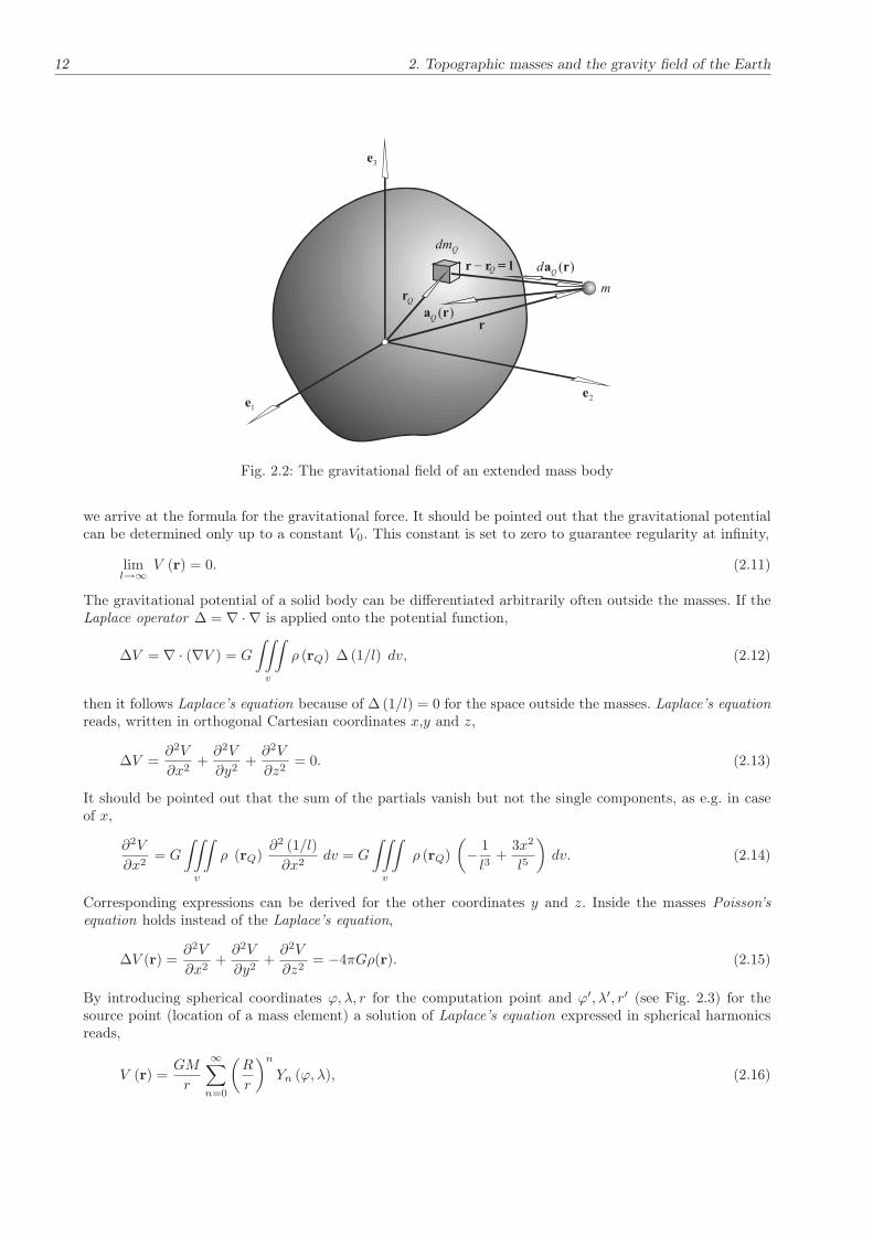
Analogously, the gravitational force field function of an extended mass, distributed in a volume describedby a certain density function ρ (rQ) can be derived. The contribution of a mass element dmQ to the forcefunction reads (Fig. 2.2),
da (r) = −GdmQ
r − rQ
| r − rQ|3=: −GdmQ
l
| l |3. (2.6)
The force function of the gravitational field of the total mass distribution can be derived as integral overthe total volume with dmQ = ρ (rQ) dv,
a (r) = −G∫∫∫
v
ρ (rQ)l
| l |3dv. (2.7)
The gravitational force is a conservative force and the gravity field strength can be determined by the gradientof a scalar function,
a(r) = ∇V (r), (2.8)
the gravitational potential,
V (r) = G
∫∫∫
v
ρ (rQ)1
| r − rQ|dv = G
∫∫∫
v
ρ (rQ)1
ldv. (2.9)
With the relation,
∇l−1 = ∇ (| r − rQ|)−1= − r − rQ
| r − rQ|3= − l
l3, (2.10)
12 2. Topographic masses and the gravity field of the Earth
1e2e
3e
Qr
r
Q-r r = l
Qdm
m
( )Qda r
( )Qa r
Fig. 2.2: The gravitational field of an extended mass body
we arrive at the formula for the gravitational force. It should be pointed out that the gravitational potentialcan be determined only up to a constant V0. This constant is set to zero to guarantee regularity at infinity,
liml→∞
V (r) = 0. (2.11)
The gravitational potential of a solid body can be differentiated arbitrarily often outside the masses. If theLaplace operator ∆ = ∇ · ∇ is applied onto the potential function,
∆V = ∇ · (∇V ) = G
∫∫∫
v
ρ (rQ) ∆ (1/l) dv, (2.12)
then it follows Laplace’s equation because of ∆(1/l) = 0 for the space outside the masses. Laplace’s equationreads, written in orthogonal Cartesian coordinates x,y and z,
∆V =∂2V
∂x2+∂2V
∂y2+∂2V
∂z2= 0. (2.13)
It should be pointed out that the sum of the partials vanish but not the single components, as e.g. in caseof x,
∂2V
∂x2= G
∫∫∫
v
ρ (rQ)∂2 (1/l)
∂x2dv = G
∫∫∫
v
ρ (rQ)
(
− 1
l3+
3x2
l5
)
dv. (2.14)
Corresponding expressions can be derived for the other coordinates y and z. Inside the masses Poisson’sequation holds instead of the Laplace’s equation,
∆V (r) =∂2V
∂x2+∂2V
∂y2+∂2V
∂z2= −4πGρ(r). (2.15)
By introducing spherical coordinates ϕ, λ, r for the computation point and ϕ′, λ′, r′ (see Fig. 2.3) for thesource point (location of a mass element) a solution of Laplace’s equation expressed in spherical harmonicsreads,
V (r) =GM
r
∞∑
n=0
(R
r
)n
Yn (ϕ, λ), (2.16)

2.1. The gravity potential and its derivatives 13
with Laplace’ surface spherical harmonics of degree n,
Yn (ϕ, λ) =1
M
∫∫∫
v
(r′
R
)n
Pn (cosψ) ρ (r′) dv =
n∑
m=0
((cnm cosmλ+ snm sinmλ)Pnm (sinϕ)). (2.17)
The functions Pnm(sinϕ) are the fully normalized Legendre functions of degree n and order m. The co-
xe
ye
ze
J
l
r
P
Q
l¢
P¢Q¢
J¢
y
¢rl
Fig. 2.3: Spherical coordinates for computation and source point
efficients cnm, snm represent the fully normalized spherical harmonic coefficients. M is the total mass ofthe Earth and R the mean radius of the Earth. If the density function inside the Earth is known, then thepotential coefficients cnm, snm can be determined also by the following integrals (with the Kronecker symbolδ0m),
cnm =(2 − δ0m)
M
(n−m)!
(n+m)!
∫∫∫
v
(r′
a
)n
Cnm (ϕ′, λ′) ρ (r′) dv,
snm =2 (1 − δ0m)
M
(n−m)!
(n+m)!
∫∫∫
v
(r′
a
)n
Snm (ϕ′, λ′) ρ (r′) dv.
(2.18)
2.1.3 The potential of the topographical and compensating masses
Let us start with the gravitational potential induced by the topographic masses above the geoid (Martinec1998),
V t(r)∣∣r=rP
= G
∫∫
σ
rg(Q)+H(Q)∫
ξ=rg(Q)
ρt(ϕQ, λQ, ξ)
l(r, ξ, ψ)
∣∣∣∣
r=rP
ξ2dξdσ, (2.19)
with
l :=√
r2P + ξ2 − 2rP ξ cosψ, (2.20)

14 2. Topographic masses and the gravity field of the Earth
and the three dimensional (3-D) density function of the topographic masses, ρt(ϕQ, λQ, ξ). The quantityξ is the geocentric radius of the mass element and dσ = cosϕQdϕQdλQ the surface element in sphericalcoordinates. The geocentric angle ψ is the spherical distance between the radius vectors of the computationpoint rP (rP , ϕ, λ) and the integration point rQ(rQ, ϕQ, λQ). It is given by
cosψ = sinϕ sinϕQ + cosϕ cosϕQ cos(λQ − λ). (2.21)
The integration in Eq. (2.19) is performed over the topographic masses bounded by the radius of the geoidrg and the Earth surface rg + H, where H stands for the topographic (orthometric) heights. It is a well-known fact that the topographical masses generate a rough gravitational field with an equipotential surfaceundulating by hundreds of meters with respect to the level ellipsoid. Since the undulations of the geoid aresignificantly smaller, compensation mechanisms of the topographical masses must exist which reduce thegravitational effects of the topographic masses. These mechanisms are most probably connected with lateralmass heterogeneities of the crust but also with deep dynamic processes (Matyska 1994). Frequently appliedare more or less idealized compensation models which are described in chapter 3.
The gravitational potential of the compensation masses can be given also by Newton’s integral as follows:
V c(r)|r=rP= G
∫∫
σ
r2∫
ξ=r1
∆ρt(ϕQ, λQ, ξ)
l(r, ξ, ψ)
∣∣∣∣r=rP
ξ2dξdσ, (2.22)
where the integration is performed over all masses for the actual compensation model with the (3-D) densityfunction ∆ρt(ϕQ, λQ, ξ), which indicates the difference between a mean density and the actual density. Theradial integration limits r1, r2 indicate the lower and upper bounds of the actual compensation masses anddepend on the applied compensation model (see chapter 3).
2.1.4 The gravitational field of a single mass layer
If the attracting masses are assumed to form a layer, or a coating on a certain closed surface σ, with athickness approaching to zero, then the surface density reads (Fig. 2.4),
kQ := k(rQ) =dmQ
dσ, (2.23)
where dσ is the surface element and kQ the single layer density. The potential of this surface of masses at acertain computation point P is given by
V (r) = G
∫∫
σ
kQ1
ldσ, (2.24)
where l is the distance between the surface element dσ and the computation point under consideration.
On the surface σ the potential V is continuous, but there are discontinuities of the first derivatives dependingon the derivation direction e. The limit of the first derivative approaching from an external point Pa to apoint Pσ at the surface σ is called the external derivative (Fig. 2.4),
limPa→Pσ
dV
de= − lim
Pa→Pσ
G
∫∫
σ
kQe · ell2a
dσ =:dVade
, (2.25)
and from an internal point Pi to a point Pσ at the surface σ the internal derivative,
limPi→Pσ
dV
de= − lim
Pi→Pσ
G
∫∫
σ
kQe · ell2i
dσ =:dVide
. (2.26)

2.1. The gravity potential and its derivatives 15
R( , )e le
s
=Q
dm k dsQ
al
il
sl
le
le
le
e
e
e
n
aP
sP
iP
sPk
l
R( , )e lel
R( , )e lel
Fig. 2.4: Potential of a material surface
The derivative at a point Pσ at the surface σ is called the direct derivative,
dV
de
∣∣∣∣σ
= G
∫∫
σ
kQd(1/lσ)
dedσ = − G
∫∫
σ
kQe · ell2σ
dσ =:dVσde
. (2.27)
If the vector n is the outer normal of the surface σ at point Pσ with the surface density kσ := kPσin this
point, the external derivative can be written in the form
dVade
= − G
∫∫
σ
kQe · ell2σ
dσ − 2πG kσn · e, (2.28)
and the internal derivative, respectively,
dVide
= − G
∫∫
σ
kQe · ell2σ
dσ + 2πG kσn · e. (2.29)
The direction derivative of a single layer shows a jump at the layer in the size of
dVade
− dVide
= − 4πGkσn · e, (2.30)
and the direct derivative is the arithmetic mean between external and internal derivatives,
dVσde
=1
2
(dVade
+dVide
)
= −G∫∫
σ
kQn · el2σ
dσ. (2.31)

16 2. Topographic masses and the gravity field of the Earth
The potential V of a single layer is regular at infinity,
liml→∞
V (r) = 0, (2.32)
satisfies everywhere Laplace’s equation,
∆V (r) = 0, (2.33)
except on σ itself, and is continuous everywhere together with all its derivatives.
2.2 The geodetic boundary value problems
2.2.1 Gravitational field and gravity field
The force acting on a test mass at the Earth’s surface is the resultant of the gravitational force and thecentrifugal force of the Earth. The centrifugal force acting on a mass m can be determined as follows:
C = mω2p, (2.34)
with the vector p = (x, y, 0) and the Earth’s angular velocity ω. Then the total force is given by
G(r) = F(r) + C(r). (2.35)
The first term of Eq. (2.35) is the gravitational force and the second term the centrifugal force which can bewritten as follows:
C(r) = mc(r), (2.36)
where c(r) is the centrifugal field strength. It is given by
c(r) = C(r)/m = ω2p. (2.37)
The resultant of the gravitational field strength and the centrifugal field strength is the gravity accelerationor simply the gravity vector,
g(r) = a(r) + c(r). (2.38)
The gravity potential is the sum of the gravitational potential and the centrifugal potential,
W (r) = V (r) + Z(r) = G
∫∫∫
v
ρ
ldv +
1
2ω2(x2 + y2). (2.39)
Since Z is an analytic function, the discontinuities of W are those of V : the second derivatives have jumpsat discontinuities of the density function. Any linear function of the gravity potential can be calculated byapplying the linear operator L as follows:
L(W (r)) = G
∫∫∫
v
L(ρ
l
)
dv + L
(1
2ω2(x2 + y2)
)
. (2.40)
An example of such an operator is the Nabla operator ∇. When applied to Eq. (2.40) it gives the gravity g:
g(r) = ∇W = G
∫∫∫
v
∇(ρ
l
)
dv + ∇(
1
2ω2(x2 + y2)
)
. (2.41)

2.2. The geodetic boundary value problems 17
reference (level)ellipsoid
equipotential surfaces
of the normal field U
Qr
Pr
Qg
g
Q
Pgeoid
0W
0U
w equipotential surfaces
of the gravity field W
N
Fig. 2.5: Gravity field and normal field
The magnitude g of the vector g is frequently called gravity in the narrower sense.
Again, the potential of the Earth can be introduced using a spherical harmonic expansion as follows (Heis-kanen and Moritz 1967):
W (r) =GM
r
(
1 +∞∑
n=2
(R
r
)n n∑
m=0
(cnm cosmλ+ snm sinmλ)Pnm(sinϕ)
)
+ω2r2
3(1 − P2(sinϕ)) , (2.42)
with the mass of the Earth M and the mean radius R. The coefficients cnm, snm are defined in Eq. (2.18).
Applying the Laplace operator to the gravity potential results in,
∆W (r) = −4πGρ+ 2ω2, (2.43)
which is the well-known Poisson’s differential equation. For the space outside the masses it reads,
∆W (r) = 2ω2. (2.44)
2.2.2 Normal figure and normal field
For linearization tasks the actual gravity field can be approximated by a model gravity field generated by alevel ellipsoid. This ellipsoid serves as a reference and is also an approximation of the mathematical figureof the Earth, the geoid or the quasi-geoid. The reference ellipsoid has the same mass M as the actual Earth.Its center coincides with the center of the Earth and it rotates with the same angular velocity ω as thereal Earth. The gravity field generated by this model is fully described by four parameters a,GM, J2, ω, thedefining parameters of a Geodetic Reference System (GRS). Its gravity potential can be expressed as follows:
U(r) =GM
r
(
1 −∞∑
n=1
(a
r
)nn∑
m=0
(c′nm cosmλ+ s′nm sinmλ)Pnm(sinϕ)
)
+ω2r2
3(1 − P2(sinϕ)) , (2.45)
where c′nm and s′nm are the fully normalized coefficients of the reference ellipsoid and a its equatorial radiusof the reference ellipsoid. It is sufficient to calculate these coefficients up to degree six or eight as the values

18 2. Topographic masses and the gravity field of the Earth
of higher degree tend to zero (Rapp 1982). Because of its symmetries, the normal potential is described onlyby an even degree zonal harmonic expansion. The zonal coefficients can be determined through,
c′n0 = − Jn√2n+ 1
, (2.46)
with the coefficients
J2 =2
3
[
f
(
1 − 1
2f
)
− 1
2m
(
1 − 2
7f +
11
49f2
)]
, (2.47)
J4 = − 4
35f
(
1 − 1
2f
)[
7f
((
1 − 1
2f
)
− 5m
(
1 − 2
7f
))]
, (2.48)
J6 =4
21f2(6f − 5m), (2.49)
and the flattening f of the reference ellipsoid and the parameter m, defined by
m =ω2a3(1 − f)
GM. (2.50)
Applying the Nabla operator to the normal gravity potential leads to the normal gravity vector,
∇U(r) = γ(r). (2.51)
The application of the Laplace operator yields
∆U(r) = 2ω2. (2.52)
Eq. (2.52) represents Poisson’s differential equation for the normal gravity potential in mass free space.
2.2.3 The boundary value problem of Stokes
In case of Stokes’ boundary value problem the equipotential surface of the gravity field in sea level, the geoid,is selected as boundary surface. The points at the geoid are projected onto the reference (level) ellipsoidalong the ellipsoidal normals (Fig. 2.5). The ellipsoidal coordinates, latitude and longitude, of the geoidpoints are considered to be known. The vertical distance between two points, the geoid height or undulationN , is unknown and has to be determined as solution of Stokes’ problem. The reference ellipsoid is a levelellipsoid, that means, the ellipsoidal surface is an equipotential surface of the normal field as explained inthe last section. The normal figure (ellipsoidal surface) and the normal field are approximations of the geoidand the gravity field, respectively. The disturbing gravity potential T is defined as the difference betweenthe gravity potential and the normal potential,
T (r) = W (r) − U(r). (2.53)
The disturbing potential and the geoid height are the unknowns of the boundary value problem of Stokeswhile the (scalar) gravity values at the geoid, g = g (P ), are considered to be the known (measured) quantities.The disturbing potential T is regular at infinity and has to be harmonic outside the boundary surface tofulfil the Laplace equation,
∆T (r) = 0. (2.54)
This will be achieved by removing all masses outside the geoid; the changes have to be corrected properly asexplained in the following chapters. A linear relation in spherical approximation between the gravity valuesat the geoid, gP , and the disturbing potential T , the so-called Fundamental equation of Physical Geodesy(Fig. 2.6),
∆g = gP − γQ = −∂T∂r
∣∣∣∣Q
− 2
rTQ, (2.55)

2.2. The geodetic boundary value problems 19
with the gravity anomalies ∆g. The linearization provides also a relation between the geoid height and thedisturbing potential (Theorem of Bruns),
N =TQγ, (2.56)
with a mean normal value γ (Somigliana 1929).
The solution of the Laplace equation (2.54) with the boundary condition (2.55) is the Stokes formula,
T (r, ϕ, λ) = T0 (r, ϕ, λ) + T1 (r, ϕ, λ) +R
4π
∫∫
s
∆g′ (ϕ′, λ′) S (r, ψ) ds, (2.57)
with the terms,
T0 (r, ϕ, λ) = −R2
r〈∆g′ (ϕ, λ)〉 , (2.58)
and
T1 (r, ϕ, λ) =GM
r2RX1 (ϕ, λ) , (2.59)
as well as the Stokes-Pizzetti function S (r, ψ). The quantity 〈∆g′〉 is the mean value of the gravity anomaliesover the Earth,
〈∆g′〉 :=1
4π
∫∫
s
∆g′ (r, ϕ′, λ′) ds, (2.60)
and X1 (ϕ, λ) is the Laplace surface spherical harmonic of degree n = 1,
X1 (ϕ, λ) = c10C10 (ϕ, λ) + c11C11 (ϕ, λ) + s11S11 (ϕ, λ) . (2.61)
The Stokes formula reads at the boundary surface, the geoid, in spherical approximation by setting r → R:
P( rj,l, )
Earth surface
reference ellipsoid0U
N
Qr
Pr
Q PB B=
Qg
g
Q
0Wgeoid
Fig. 2.6: Relation between the surface of the Earth, the geoid and the reference ellipsoid
T (ϕ, λ) = T (R,ϕ, λ) = T0 (ϕ, λ) + T1 (ϕ, λ) +R
4π
∫∫
s
∆g (ϕ′, λ′) S (ψ(ϕ, λ;ϕ′, λ′)) ds, (2.62)

20 2. Topographic masses and the gravity field of the Earth
with
T0 (ϕ, λ) =GδM
R= −R 〈∆g (ϕ, λ)〉 , (2.63)
and
T1 (ϕ, λ) =GM
R2(cosϕ cosλ ex + cosϕ sinλ ey + sinϕ ez) · rCM , (2.64)
where the Stokes-Pizzetti function S (r, ψ) becomes the Stokes function S (ψ). For the geoid height it followsaccording to the Theorem of Bruns,
N (ϕ, λ) =T (ϕ, λ)
γ= N0 (ϕ, λ) +N1 (ϕ, λ) +
R
4πγ
∫∫
σ
∆g′ (ϕ′, λ′) S (ψ(ϕ, λ;ϕ′, λ′)) dσ. (2.65)
Because of the fact that the masses outside the geoid have to be removed or shifted inside the boundarysurface these geoid heights are the heights of a preliminary boundary surface, the co-geoid.
2.2.4 Topographic isostatic effects in Stokes’ boundary value problem
The solution of the boundary value problem of Stokes by solving the Laplace equation requires that thegravity potential outside the geoid is harmonic. As pointed out already, it is necessary to remove the topo-graphic masses or shift them inside the boundary surface. Then it is possible to solve the boundary valueproblem based on Laplace’s equation. Obviously, the solution has to be corrected afterwards to restore theoriginal situation, that means, the determination of the geoid inside the masses. Therefore, the reductionand correction steps require a detailed knowledge of the topographic masses.
The effects of the topographic and the isostatic or condensed masses on the geoid heights are evaluated asthree separate contributions: the direct topographic effect on the gravity, the primary indirect topographiceffect on the geoid and the secondary indirect topographic effect on the gravity (e.g., Novàk et al. 2001) incase of the gravity at the surface of the Earth. For airborne gravimetry where gravity disturbances at flightlevel are considered as observations, only the direct and the secondary indirect topographic effects have tobe considered. The harmonized disturbing potential can be determined for any point in space by (Martinecet al. 1993),
Th(r) = T (r) − δV (r),
Th(r, ϕ, λ) = T (r, ϕ, λ) − δV (r, ϕ, λ),(2.66)
with the disturbing potential T of the Earth’s gravity field, and the direct topographic-isostatic effect on thegravitational potential δV (r, ϕ, λ). The latter one is the difference between the gravitational potential of thetopography V t(r, ϕ, λ) and the gravitational potential of the isostatic or condensed masses V c(r, ϕ, λ),
δV (r, ϕ, λ) = V t(r, ϕ, λ) − V c(r, ϕ, λ). (2.67)
The spherical coordinates r,ϕ and λ of the computation point at the surface of the Earth or at airbornealtitude refer to a geocentric coordinate system.
The geoid heights of the co-geoid can be derived by Bruns’ theorem from the harmonized disturbing potentialas solution of the geodetic boundary value problem and a correction term on the co-geoid height, the primaryindirect topographic-isostatic effect PITE(R,ϕ, λ),
N(ϕ, λ) =T (R,ϕ, λ)
γ0(ϕ)=Th(R,ϕ, λ)
γ0(ϕ)+δV (R,ϕ, λ)
γ0(ϕ)=:
Th(R,ϕ, λ)
γ0(ϕ)+ PITE(R,ϕ, λ), (2.68)
with the normal gravity γ0(ϕ) at the level ellipsoid.

2.2. The geodetic boundary value problems 21
topography with isostatic mass compensation
geoid
topography
isostatic masses
change of the geoid by mass removal or mass redistribution
geoid
co-geoid
PITE
PITE
determination of the geoid inside the masses
geoid
co-geoid
cV
tV
- Stokes formula:
( )4
h hR
N g S d
s
y spg
= Dòò
Determination of the co-geoid
D ® Dh h
cg g
Downward continuation of surfacegravity anomalies from the Earth
surface down to the geoid
- gravity values at the Earth surface:
- gravity values at the Earth surface:
- gravity values at the Earth surface:
- gravity values at the Earth surface:
Measurement
sg
- direct topographic-isostatic mass effectson the gravity potential
- direct topographic-isostatic mass effecton the gravity:
- secondary indirect topographic-isostaticmass effect on the gravity:
d = -t cV V V
d¶ ¶ =V r DTE
d =2 V r SITE
Determination of topographic-isostaticeffects on the gravity anomalies
D = D + +hg g DTE SITE
= +hN N PITE
Determination of the geoid
- topographic-isostatic mass effects on thegeoid height (primary indirect topographic-isostatic effect)
Determination of the surface gravityanomalies
s gg
¶æ öD = - + +ç ÷¶è ø
...g g Hh
Fig. 2.7: Flow chart of the geoid determination procedure considering the various topographic-isostatic effects
By applying the negative radial derivative to Eq. (2.66), the corresponding topographical effect on gravitycan be obtained as follows:
δgh(r, ϕ, λ) = −∂Th(r, ϕ, λ)
∂r= −∂T (r, ϕ, λ)
∂r+∂δV (r, ϕ, λ)
∂r=: δg(r, ϕ, λ) +DTE(r, ϕ, λ), (2.69)
where δg and δgh are the gravity disturbances of the real gravity field and the harmonized gravity field,respectively, and DTE(r, ϕ, λ) is the direct topographic-isostatic effect on gravity. The direct and primaryindirect topographic-isostatic effects given in Eq. (2.68) and Eq. (2.69), respectively, represent the effect ofthe topographic and isostatic masses for geoid determinations based on airborne gravity measurements. Sincethe gravity disturbances δg differ from the gravity anomalies ∆g only by the vertical change of normal gravityalong the separation between the actual equipotential surface and the corresponding normal equipotentialsurface, the following expression can be obtained for points at the surface of the Earth:
∆gh(r, ϕ, λ) = ∆g(r, ϕ, λ) +∂δV (r, ϕ, λ)
∂r(ϕ, λ)+
2
rδV (r, ϕ, λ)
=: ∆g(r, ϕ, λ) +DTE(r, ϕ, λ) + SITE(r, ϕ, λ).
(2.70)
22 2. Topographic masses and the gravity field of the Earth
The second term at the right hand side of Eq. (2.71) represents the direct topographic-isostatic effect ongravity, DTE(r, ϕ, λ), and the third term the secondary indirect topographic effect on gravity, SITE(r, ϕ, λ).
To determine the geoid, the downward continuation of the gravity anomalies, defined in Eq. (2.71), from thetopography to the geoid has to be performed according to (Novàk 2000):
∆ghc (R,ϕ, λ) = ∆gh(r, ϕ, λ) +D∆gh(ϕ, λ), (2.71)
where D∆gh(ϕ, λ) is the downward continuation term. The geoid can be determined by Eq. (2.65). If themasses of the reference ellipsoid and the Earth are identical and the origin of the terrestrial reference frameis located at the center of mass of the Earth then the first two terms become zero and the solution reads asfollows,
Nh = N0 =R
4πγ
∫∫
s
∆ghc (R,ϕ, λ)S(ψ)ds, (2.72)
here N0 is the harmonized undulation of the co-geoid referred to the reference ellipsoid and S(ψ) the Stokes’function given by:
S(ψ) =1
sin(ψ/2)− 6 sin(ψ
/2) + 1 − 5 cosψ − 3 cosψ ln
(sin(ψ
/2) + sin2(ψ/2)
). (2.73)
Finally, the geoid heights can be restored by the formula:
N = Nh + PITE = Nh + δN. (2.74)
The computation steps are shown in the flow chart of Fig. 2.7.
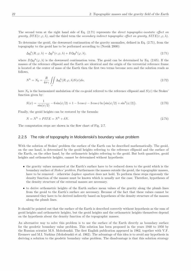
2.2.5 The role of topography in Molodenskii’s boundary value problem
With the solution of Stokes’ problem the surface of the Earth can be described mathematically. The geoid,on the one hand, is determined by the geoid heights referring to the reference ellipsoid and the surface ofthe Earth, on the other hand, by the orthometric heights referring to the geoid. But both quantities, geoidheights and orthometric heights, cannot be determined without hypothesis:
• the gravity values measured at the Earth’s surface have to be reduced down to the geoid which is theboundary surface of Stokes’ problem. Furthermore the masses outside the geoid, the topographic masses,have to be removed – otherwise Laplace equation does not hold. To perform these steps rigorously thedensity function of the masses must be known which is usually not the case. Therefore, hypotheses ofthe density structure of the external masses are necessary.
• to derive orthometric heights of the Earth surface mean values of the gravity along the plumb linesfrom the geoid to the Earth’s surface are necessary. Because of the fact that these values cannot bemeasured they have to be derived indirectly based on hypotheses of the density structure of the massesalong the plumb lines.
It should be pointed out that the surface of the Earth is described correctly without hypothesis as the sum ofgeoid heights and orthometric heights, but the geoid heights and the orthometric heights themselves dependon the hypothesis about the density function of the topographic masses.
An alternative way to solve this problem is to use the surface of the Earth directly as boundary surfacefor the geodetic boundary value problem. This solution has been proposed in the years 1940 to 1950 bythe Russian scientist M.S. Molodenskii. The first English publication appeared in 1962, together with V.F.Eremeev and M.I. Yurkina (Molodenskii et al. 1962). The advantage of this idea is to avoid any hypothesis inderiving a solution to the geodetic boundary value problem. The disadvantage is that this solution strategy

2.2. The geodetic boundary value problems 23
causes much more mathematical problems than in case of the Stokes’ problem. The first obvious differenceis that the boundary surface of Molodenskii’s problem is not an equipotential surface with normals directedto the gravity vector. Instead the boundary surface is an arbitrary not even continuous function. It is also anon-linear problem similar to Stokes’ problem, but the linearization causes much more problems because ofthe fact that the geoid deviates from the reference ellipsoid only by a maximum of 100 m, while the surfaceof the Earth shows ellipsoidal heights of up to approximately 9000 m. Furthermore, Molodenskii’s problemis not only a free boundary value problem but also a so-called oblique boundary value problem because ofthe fact that the gravity vector is usually not orthogonal to the boundary surface.
A consequence of the large deviations of the surface of the Earth (considered as boundary surface) from thereference ellipsoid is that an approximation of the boundary surface has to be introduced which is closer tothe boundary surface. This approximation is the telluroid, which is referred to the reference ellipsoid by atype of heights which can be determined without hypothesis, the so-called normal heights. The deviationsof the surface of the Earth and the telluroid, the height anomalies, are in the size of the geoid heights. Ifthe points of the surface of the Earth are referred to a vertical reference surface by the normal heights –similar to the geoid in case of orthometric heights – then one arrives at the quasi geoid which coincidesapproximately with the geoid (Fig. 2.10). In the following, we will only give the solution of Molodenskii’s
gn
gn
Qg
Pg
V
H
QU const=
PW const=
Q PB B=telluroid
normal field
gravity field
height anomaly
normal height
ellipsoid normal
P
Q
Earth surface
V
H
gravity normal at the surface point
normal of the normalfield at point
:P
:Q
reference ellipsoid
Fig. 2.8: Relation between the surface of the Earth, the telluroid and the reference ellipsoid
boundary value problem in form of the so-called Molodenskii series where the first approximation is identicalwith the solution of Stokes problem with a slightly different definition of the gravity anomalies used in thesolutions (Heiskanen and Moritz 1967; Klees 1992; Lehmann 1994),
T =∞∑
n=0
Tn, (2.75)
with
Tn =R
4π
∫∫
σ
GnS (ψ) dσ for n = 0, 1. (2.76)
and
Tn =R
4π
∫∫
σ
G0 S (ψ) dσ − R2
4µ
∫∫
σ
(h− hP )2
l30Gn−2dσ for n ≥ 2. (2.77)

24 2. Topographic masses and the gravity field of the Earth
The functions Gn can be determined by the following formulae,
G0 = ∆g, (2.78)
with the surface gravity anomalies ∆g = gP − γQ and
G1 =R2
2π
∫∫
σ
h− hPl30
G0dσ, (2.79)
G2 =R2
2π
∫∫
σ
h− hPl30
G1dσ +G0 tan2 β, (2.80)
G3 =R2
2π
∫∫
σ
h− hPl30
G2dσ +G1 tan2 β − 3R2
4π
∫∫
σ
(h− hP )3
l50G0dσ, (2.81)
where β is the maximum inclination of the terrain, hP the ellipsoidal height of the computation point and hthe ellipsoidal height of the integration point (for the notation refer also to Moritz 1965, 1980).
The height anomalies can be derived subsequently by applying Bruns’ theorem
ζ =T
γ. (2.82)
The first two terms of the series Eq. (2.75) represent an approximation of the solution of Molodenskii’sproblem which is sufficient for many applications. The disturbance potential reads,
T ≈ T0 + T1 =R
4π
∫∫
σ
(∆g +G1) S (ψ) dσ, (2.83)
which can be used to derive the height anomalies again by Bruns’ theorem,
ζ ≈ ζ0 + ζ1 =R
4πγ
∫∫
σ
∆g S (ψ) dσ +R
4πγ
∫∫
σ
G1 S (ψ) dσ. (2.84)
The term G1 can be considered as terrain correction with constant density (Moritz 1968),
G1 =1
2GρR2
∫∫
σ
(h− hP )2
l30dσ. (2.85)
The solution of the boundary value problem of Molodenskii does not need any assumptions about the densityof the topography and the crust as it depends on the free-air anomalies at the surface of the Earth. But itis known that the free-air anomalies are small and strongly dependent on the roughness of the topography,so that their interpolation is very inaccurate (Heiskanen and Moritz 1967). Therefore, it is preferable alsoin case of Molodenskii’s boundary value problem to make use of the well-known advantages of the Bouguerand isostatic anomalies. These anomalies are smoother and more representative than the free air anomaliesand can be interpolated more easily and more accurately.
To take the effect of the topographic-isostatic masses into account, we start with Eq. (2.66) as it representsthe disturbing potential by removing the topographic-isotatic masses as follows:
T r(rP , ϕ, λ) = T (rP , ϕ, λ) − δV (rP , ϕ, λ). (2.86)
With these reductions the disturbing potential will be smoother than the original one; therefore we call itregularized disturbance potential T r. In this case, the physical surface of the Earth will remain unchanged,but the telluroid will change, because its points Q are defined by UQ = WP , and the potential W at any pointP will be affected by the removing of the topographic masses. The height anomaly difference δζ between

2.2. The geodetic boundary value problems 25
Determination of topographic-isostaticeffects on gravity anomalies
- direct topographic-isostatic mass effectson the gravity potential:
- direct topographic-isostatic mass effecton the gravity:
- secondary indirect topographic-isostaticmass effect on the gravity:
d = -t cV V V
d¶ ¶ =V r DTE
d =2 V r SITE
- Molodenskii series:
( )
( )1
4
4
r rRg S d
RG S d
s
s
z D y spg
y spg
» +
+
òò
òò
Determination of the regularizedtelluroid
- gravity values at the Earth surface:
Measurement
sg
gD = -g g
- regularized gravity anomaly:
Determination of the regularizedsurface gravity anomalies
D = D + +rg g DTE SITE
rz z dz= +
Determination of the telluroid
- topographic-isostatic mass effects on theheight anomalies
topography with isostatic mass compensation
geoid
topography
isostatic masses cV
tV
ellipsoid
determination of the telluroid inside the masses
ellipsoid
geoid
telluroid
regularized telluroid
dz
change of the telluroid by mass removal or mass redistribution
geoid
ellipsoid
telluroid
regularized telluroid
dz
Fig. 2.9: Flow chart of the telluroid determination procedure considering the various topographic-isostaticeffects
the original telluroid and the regularized telluroid according to Bruns’ theorem is given by (Heiskanen andMoritz 1967),
δζ = ζ − ζr =δV
γ, (2.87)
where γ is the normal gravity on the telluroid. In this case the regularized gravity anomalies at the surfaceof the Earth will be given by:
∆gr = ∆g − δg − ∂γ
∂hδV = ∆g +DTE + SITE. (2.88)
The second term in the right hand side of Eq. (2.88) represents the direct topographical effect on gravity andthe third term the secondary indirect topographical effect on gravity, both analogously to Eq. (2.70). After
26 2. Topographic masses and the gravity field of the Earth
that the regularized height anomalies ζr are computed from the regularized gravity anomalies ∆gr by thesolution of Molodenskii’s problem according to Eq. (2.82) or approximately by Eq. (2.84),
ζr ≈ R
4πγ
∫∫
σ
∆gr S (ψ) dσ +R
4πγ
∫∫
σ
G1 S (ψ) dσ. (2.89)
Finally, the original height anomalies ζ are obtained by considering the indirect effect by inserting δζ accor-ding to Eq. (2.87):
ζ = ζr + δζ. (2.90)
The computation steps are shown in the flow chart of Fig. 2.9.
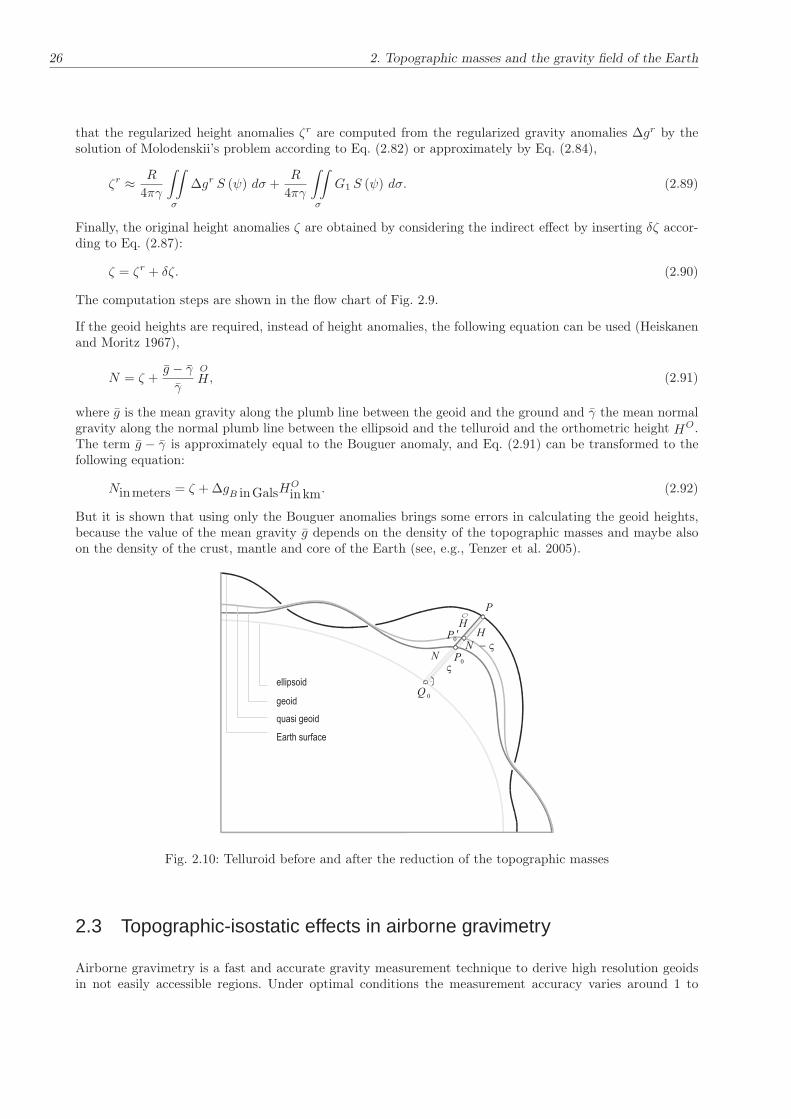
If the geoid heights are required, instead of height anomalies, the following equation can be used (Heiskanenand Moritz 1967),
N = ζ +g − γ
γ
O
H, (2.91)
where g is the mean gravity along the plumb line between the geoid and the ground and γ the mean normalgravity along the normal plumb line between the ellipsoid and the telluroid and the orthometric height HO.The term g − γ is approximately equal to the Bouguer anomaly, and Eq. (2.91) can be transformed to thefollowing equation:
Ninmeters = ζ + ∆gB inGalsH
O
inkm. (2.92)
But it is shown that using only the Bouguer anomalies brings some errors in calculating the geoid heights,because the value of the mean gravity g depends on the density of the topographic masses and maybe alsoon the density of the crust, mantle and core of the Earth (see, e.g., Tenzer et al. 2005).
ellipsoid
P
geoid
quasi geoid
Earth surface
0P
0P ¢
0Q
N V-H
HO
NV
Fig. 2.10: Telluroid before and after the reduction of the topographic masses
2.3 Topographic-isostatic effects in airborne gravimetry
Airborne gravimetry is a fast and accurate gravity measurement technique to derive high resolution geoidsin not easily accessible regions. Under optimal conditions the measurement accuracy varies around 1 to

2.3. Topographic-isostatic effects in airborne gravimetry 27
2 mGal for a spatial resolution of approximately 2 km. The downward continuation of these observationsrequires a filtering of the observables to reduce the intrinsic instabilities. To ease the downward continuationof filtered data from aircraft altitude down to sea level, it is helpful to additionally apply a remove-restoretechnique (Forsberg and Tscherning 1997) based on gravity field information provided by the topographic-isostatic masses. The effects of the topographic-isostatic masses on the geoid heights from airborne gravityare evaluated as two separate contributions: the direct topographical effect on the gravity (DTE ) and the(primary) indirect topographical effect on the geoid (PITE ) (Novàk et al. 2001).
The observables of airborne gravimetry are gravity disturbances at aircraft altitude. They are defined asdifferences between the actual gravity and the normal gravity at the same point. If the gravity disturbanceson the reference ellipsoid are given and the disturbing potential is required in the space outside the masses,then we have to solve a geodetic boundary value problem of the second kind or a so-called Neumann problem.In this case, the Laplace equation for the disturbing potential,
∆T = 0, (2.93)
has to be solved, satisfying the following boundary condition (defined on the reference ellipsoid),
δg = gp − γP = −∂T∂n
, (2.94)
where n is the ellipsoidal normal and gp and γP the actual and normal gravity at the boundary surface. Incase of a spherical approximation Eq. (2.94) can be simplified as
δg = gp − γP = −∂T∂r
. (2.95)
The solution of the Neumann problem in this case is given by (e.g., Hotine 1969; Novàk et al. 2000):
T (ϕ, λ) =R+ hf
4π
∫∫
σ
δg H(ψ) dψ, (2.96)
where H(ψ) is the Hotine function and hf is the height of the aircraft. It can be given as a closed formulaas follows (Hotine 1969):
H(ψ) =
∞∑
n=0
(2n+ 1)
(n+ 1)Pn(cosψ) = cosec (1/2ψ) + ln (1 + cosec (1/2ψ)) . (2.97)
This equation includes the zero and the first order terms of the spherical harmonic expansion of the disturbingpotential. If the mass of the Earth is assumed to be equal to the mass of the reference ellipsoid and the centerof the Earth is assumed to coincide with the origin of the reference system, then Hotine’s function can besimplified as following:
H(ψ) =
∞∑
n=2
(2n+ 1)
(n+ 1)Pn(cosψ) = cosec (1/2ψ) + ln (1 + cosec (1/2ψ)) − 1 − (3/2) cosψ. (2.98)
If we want to remove the topographic-isostatic masses then we have to follow, in principle, the proceduredescribed in Fig. 2.7. The observations δg have to be corrected by the DTE at aircraft altitude to get theharmonized gravity disturbance at aircraft altitude,
δgh = δg −DTE (R+D,ϕ, λ) (2.99)
with
δgh =∂Th(R+D,ϕ, λ)
∂r, (2.100)
δg =∂T (R+D,ϕ, λ)
∂r, (2.101)

28 2. Topographic masses and the gravity field of the Earth
DTE (R+D,ϕ, λ) :=∂δV (r, ϕ, λ)
∂r
∣∣∣∣r=R+D
=∂V t
∂r− ∂V c
∂r, (2.102)
where δV (r, ϕ, λ) is the difference between the gravitational potential of the topography V t and the gravita-tional potential of the isostatic or condensed topographic masses, V c. In the following step, the harmonizedgravity disturbances at aircraft altitude have to be downward continued to the boundary surface,
δgh → δghc . (2.103)
Then the Hotine integral is applied to give the co-geoid as follows:
Nh(ϕ, λ) =R
4π
∫∫
σ
δghcH(ψ)dψ. (2.104)
Finally, the primary indirect topographical effects are added to give the geoid heights,
N(ϕ, λ) = Nh(ϕ, λ) + PITE, (2.105)
with
PITE =δV
γ. (2.106)
2.4 Topographic-isostatic mass effects in satellite application
The dedicated satellite gravity missions CHAMP (Reigber et al. 1999) and GRACE (Tapley et al. 2004) aswell as ESA’s GOCE mission, to be launched in 2007, (ESA 1999) will improve our knowledge of the Earth’sgravity field in the long, medium and short wavelength ranges. The novel measurement techniques areSatellite-to-Satellite Tracking (SST) either in the high-low, the low-low or the Precise Orbit Determination(POD) mode and Satellite Gravity Gradiometry (SGG), respectively. After an operational period of only afew months after its launch in July 2000, a global gravity field model has been generated from the CHAMPGPS-SST data, which recovers the long- to medium-wavelength part of the gravity field by one order ofmagnitude more accurate than during the last decades of classical satellite geodesy (Reigber et al. 2002).As a result of ultra-precise ranging between satellites, a further breakthrough in accuracy and resolutionhas been achieved with the gravity field models derived from data generated by the twin-satellite missionGRACE, launched in 2002 (Mayer-Gürr et al. 2006). Meanwhile, monthly snapshots of the gravity field havebeen computed, allowing for the first time the resolution of temporal variations over a wide spatial andtemporal spectrum.
The innovative character of these missions consists in the more or less complete coverage with observations bythe Global Positioning System (GPS) and the continuous very precise line-of-sight range-rate measurementsby GRACE, as well as the measurement of the gravity gradients by a three-dimensional gravity gradiometerwithout interruption in the case of GOCE. To prevent the observations from non-gravitational constituents,the surface forces are either measured and considered in a pre-processing step or will be compensated by adrag-free control system directly, as in case of GOCE.
2.4.1 Improperly posed problems in satellite geodesy
A critical point of the determination of gravity field parameters from observations at satellite altitude is thedownward continuation of the high-precise SST data and the SGG observations. It is well-known that thesegravity field recovery problems are improperly posed problems, that means, small changes in the observationsproduce large effects in the solutions. These problems usually require a proper regularization to receive stablerecovery results. The basic principle behind regularization, e.g., in case of Tichnov’s regularization method,is a balancing procedure between observation noise and unknowns. Regularization of unstable problems is

2.4. Topographic-isostatic mass effects in satellite application 29
especially critical in those cases where the noise is intermingled with the signal content in the observations.Some contributions of the gravity signal are well known a-priori. Therefore, it is advantageous if those signalparts are reduced prior to the downward continuation and restored after the recovery procedure. In this case,we can anticipate that the high frequent part in the observations is mainly caused by the observation noisewhich can be filtered without loosing gravity field signals.
One important source of high frequent signal constituents in the satellite observations is caused by thetopographical masses and its isostatic compensation. Nowadays, very precise digital elevation models (DEM)of land and sea (bathymetry) are available. The effects of the topographic-isostatic masses on the gravityfield determinations from the new in-situ satellite gravity missions are evaluated also in this case as twoseparate contributions: the direct topographical effect on the gravity (DTE ) and the (primary) indirecttopographical effect on the geoid (PITE ). The application of the direct topographic-isostatic effects onthe observables at satellite altitude acts as a smoothing of the observations which simplifies the downwardcontinuation procedure. Here we give only some basic information of the recovery models – the numericaleffects in satellite altitude will be discussed later.
2.4.2 The use of topographic-isostatic mass effects in the Satellite -to- Satellite Trackingtechnique
The mathematical models for global as well as regional gravity field recovery from precise kinematical orbits,high-low and low-low Satellite-to-Satellite Tracking data is based on the formulation of Newton’s equation ofmotion,
r(t) = a(t; r, r;x), (2.107)
as a boundary value problem,
r(t) = (1 − τ) rA + τrB − T 2
1∫
τ ′=0
K (τ, τ ′) a(t; r, r,x) dτ ′ (2.108)
with the integral kernel,
K (τ, τ ′) =
{
τ (1 − τ ′) , τ ≤ τ ′,
τ ′ (1 − τ) , τ ′ ≤ τ,(2.109)
the normalized time variable,
τ =t− tAT
with T = tB − tA, t ∈ [tA, tB ], (2.110)
and the boundary values
rA := r(tA), rB := r(tB), tA < tB. (2.111)
The specific force function in Eq. (2.108) with the unknown parameters x can be separated as follows,
a(t; r, r;x) = ad(t; r, r) + ∇V (t; r;x0) + ∇T (t; r;∆x). (2.112)
The quantity ad is a disturbance part, which represents the non-conservative disturbing forces, ∇V is areference part, representing the long wavelength gravity field features x0 and ∇T is an anomalous part,modelling the high frequent refinements ∆x to the low frequent gravity field parameters x0 of the globalmodel.
In case of the analysis of precisely determined kinematical orbits according to the POD technique the Eq.(2.108) together with Eq. (2.112) represents the physical model. It has to be supplied by a properly selected

30 2. Topographic masses and the gravity field of the Earth
stochastic model, where both models together build the mathematical model to determine corrections to thefield parameters. This model has been successfully applied for the determination of the gravity field modelITG-Champ01 (details can be found in Mayer-Gürr et al. 2005).
If precise intersatellite functionals such as line-of-sight measurements between two satellites, following eachother on the same orbit are available, as in case of the GRACE mission, the mathematical model for rangeobservations can be derived by projecting the relative vector to the line-of-sight connection,
ρ(τ) = e12(τ) · (r2(τ) − r1(τ)) . (2.113)
Analog formulae can be derived for range-rates and range accelerations. The quantity e12 is the unit vectorof the line-of-sight direction of the two GRACE satellites with the positions r1(τ) and r2(τ). This vector isknown with high accuracy, assuming that the satellite positions are measured with an accuracy of a few cmand taking into account the distance of approximately 200km between the two satellites. Nevertheless, thisaccuracy is not adequate to the extremely high accuracy of the range measurements in the size of some µm.Therefore, a model refinement is necessary which improves implicitly also the relative orbit. The arcs of thesatellites are fitted to the observables such that the unknown gravity field parameters are solved for whilethe quadratic norm of the observation residuals is minimized. To end up with a stable solution, a regularizedsolver of Tichnov type has to be applied, where the regularization parameter is preferably computed accordingto the variance component estimation procedure due to Koch and Kusche (2003). Further details to thephysical model of the gravity field recovery technique based on GRACE low-low SST data can be found alsoin Mayer-Gürr (2006) and in Mayer-Gürr et al. (2006).
2.4.3 The use of topographic-isostatic mass effects in Satellite Gravity Gradiometry
GOCE (Gravity Field and Steady-State Ocean Circulation Explorer) has the potential of deriving the globalgravity field with unprecedented accuracy in the high resolution spectral part. The usual way is to model thegravity field by spherical harmonics. A disadvantage of this kind of gravity field representation is the lack offlexibility in modelling the inhomogeneous gravity field features in specific regions. An alternative approach isto determine a global gravity field solution, based on GRACE SST observations up to a moderate degree andimprove this global solution in selected regions by an adapted regional recovery procedure. The individualgravity field features in these regions can be modelled by space localizing base functions such as sphericalspline functions. The advantage of this method is the possibility of adjusting the spline representation andthe recovery procedure according to the regional gravity field structures and the specific data distribution. Inthe present case, the consideration of topographic-isostatic effects as discussed above is even more importantthan in case of SST because of the higher satellite altitudes of the latter one.
The observations of the GOCE gradiometer are the second derivatives of the gravitational potential ∇∇V (P ).They are observed along the satellite orbit at a regular sampling rate. Every observation constitutes anobservation equation if the gravity field is parameterized, adapted to the specific task. The parameterizationof the potential is performed in terms of spherical harmonics for the global solution, in case of a regionalgravity field recovery the potential has to be parameterized by space localizing base functions. It can bemodelled as a sum of base functions as follows:
V (rP ) =I∑
i=1
ai ϕ(rP , rQi) (2.114)
with the field parameters ai arranged in a column matrix and the base functions,
ϕ(rP , rQi) =
∞∑
n=0
kn
(R
r
)n+1
Pn(rP , rQi). (2.115)
The coefficients kn are the degree variances of the gravity field spectrum to be determined,
kn =M∑
m=0
(∆c2nm + ∆s2nm
). (2.116)

2.4. Topographic-isostatic mass effects in satellite application 31
R is the mean equator radius of the Earth, r the distance of a field point from the geocenter and Pn(rP , rQi)
are the Legendre’s polynomials depending on the spherical distance between a field point P and the nodalpoints Qi of the set of base functions. With this definition the base functions can be interpreted as isotropicand homogeneous harmonic spline functions (Freeden et al. 1998). The nodal points are generated on a gridby a uniform subdivision of an icosahedron of twenty equal-area spherical triangles. In this way the globalpattern of the spline nodal points Qi shows approximately uniform nodal point distribution (details can befound in Eicker et al. 2004).
The observation equation for gradiometer measurements is obtained by differentiating the potential twice:
∇∇V (P ) =
I∑
i=1
ai ∇∇ϕ(rP , rQ). (2.117)
The observation equations are established for short arcs over the selected regional recovery area, while thecoverage with short arcs should be slightly larger than the recovery region itself to prevent the solutionfrom geographical truncation effects. Every short arc builds a partial normal equation. To consider differentaccuracies of the short arcs these normal equations are combined by estimating a variance factor for everyarc by means of a variance component estimation such as described by Koch and Kusche (2003). In thosecases where a regularization is required, the regularization factor can be determined within the variancecomponent estimation procedure as well.

32
3. Mass models of the Earth’s topography
In chapter 2, various geodetic applications are presented which demonstrate the need or at least the usefulnessof considering the effects of topographic-isostatic masses. For this reason, the mass of the Earth must bemodeled in a satisfying way. The topographic-isostatic models with mass density information from geologicaland geophysical investigations and orthometric heights from digital terrain models can be used for geodeticapplications. These models have more or less a geophysical meaning. Other models, such as Helmert’s methodsof condensation can be used as purely mathematical approaches to remove the masses outside the geoid andshift it inside the boundary surface. In this chapter a review of the various topographic-isostatic modelsand the different data sets is given which can be used for the geodetic applications of topographic-isostaticmasses as mentioned in chapter 2:
1. digital terrain models (DTM) for modelling the shape of the topography,
2. digital density models (DDM) for modelling the spatial distribution of density in the topography anddeeper masses,
3. isostatic models for analytically modelling the Earth’s outer masses,
4. Helmert’s method of condensation as a simple model to fulfill the assumption of Stokes’ theory.
3.1 Digital terrain model
A digital terrain model (DTM) is a digital representation of the topography of the Earth, that is, by horizontalcoordinates and a numerical description of the topography heights. A large variety of digital terrain modelsis currently available. Some DTM’s only contain height information of the solid Earth surface (i.e. landheights and ocean depths), whereas others also contain information on, for instance, thicknesses of glaciersand oceanic ice shelves, or lake depths. In this investigation the digital terrain model ETOPO5 with aresolution of five arc-minutes is used for the satellite applications. ETOPO5 (Earth Topography 5-minute)is a gridded elevation (land) and bathymetry (sea floor) data set for the entire Earth at a grid spacing of5 minutes (1/12 of a degree or 300 arcseconds). The entire data set consists of a single file which has 4320columns and 2160 rows. This data set was compiled using data from many different sources by the NationalGeophysical Data Center (NGDC), which is part of the National Oceanic and Atmospheric Administration(NOAA). Most of the data set dates back to 1988, except for a small area in Canada that was re-griddedin 1990. Elevation values are stored in a flat binary file (row major, no header) as signed 2-byte integers,and are available with both the LSB (least significant byte first) and MSB (most significant byte first) byteorders. The elevation units are meters. This data set provides global coverage and can be obtained freeof charge from NGDC/NOAA. A version with a resolution of two arc-minutes (3.6 km) was published in2001. Five major data sources were assembled into the ETOPO2 data base: data derived from GLOBEDEM (Sandwell and Smith 1997), bathymetric data from the Digital Bathymetric Data Base (DBDB),from the International Bathymetric Chart of the Arctic Ocean (IBCAO) and the Digital Bathymetric DataBase with a 5 arc-minutes resolution (DBDB5) filling any gaps (Kiamehr and Söjberg 2005). For moreinformation see: www.ngdc.noaa.gov/mgg/fliers/01mgg04.html. In this investigation, for Earth surface andairborne applications the numerical tests are based on the high-resolution DTM GEBCO with one arc-minute resolution (www.ngdc.noaa.gov/mgg/gebco). The GEBCO Digital Atlas project is carried out underthe auspices of the Intergovernmental Oceanographic Commission (IOC) and the International HydrographicOrganization (IHO). It has been reviewed by the Joint IOC/IHO Guiding Committee for GEBCO; a technicalguidance is provided by the GEBCO Sub-Committee on Digital Bathymetry.

3.2. Digital density models 33
3.2 Digital density models
So far, the actual density of the Earth crust is not known; occasionally density models describe only thesurface densities, derived from geological maps. Therefore, many of the investigations performed in thepast depend on a constant density for the Earth crust. Since the actual density of the topographic massesmay differ by more than 10% from a constant density (Martinec 1993; Tziavos et al. 1996; Pagiatakis andArmenakis 1998; Kuhn 2000a, b; Huang et al. 2001), the resulting geoid models will contain significanterrors. Therefore, a 3-D digital density model (3-DDM) would be required to give a better modelling of thetopographic masses. But in practice, it is very difficult – if not impossible – to provide such models on aglobal scale. On the other hand, 2-DDM are sufficient for many geodetic applications. Nowadays, a 2-DDMis available for some regions such as for Canada (see, e.g., Pagiatikis and Armenakis 1998). In general, anyreasonable density model will give an improvement by using more realistic gravity reductions for the geoiddetermination.
3.3 Isostatic models
One of the first ideas about the equilibrium of the Earth’s outer layers originate from Leonardo da Vinci(1452-1519). He expressed interesting speculations how the Earth might response to loads on its surface.Much later, Bouguer in 1749 gave the first experimental proof for the isostasy theory during the expeditionto Quito (South America) in the year 1735 to measure the length of the meridian at the equator to derivethe eccentricity of the ellipsoidal figure of the Earth. He discovered that the attraction effects of the Andesare by far smaller than it would have been expected because of the huge visible masses. For the explanationof this phenomena Bouguer and Boscovich (1755) speculated that the mass excess of the mountains might becompensated in some way by a mass deficiency at depth (Watts 2001). Some decades later, Everest carriedout geodetic measurements in India in the years 1840 to 1859. As part of these measurements he computedthe geodetic position at a number of locations where he had already measured astronomic positions. He foundthat for the cities Kaliana and Kalianpur in the Ganges plain the latitude differences between the positionscomputed geodetically was 5.24 arc-seconds smaller than those determined astronomically. Everest concludedthat this discrepancy was not caused by the astronomical measurements; they could only be caused by thegeodetic determination of the positions. But Pratt in 1854 and Airy in 1859 disagreed; they explained thesesignificant differences by their isostatic models that they proposed before. Both came to the conclusion thatthe visible topographic masses of the Himalaya must be compensated in some way. This idea was the samewhich has been expressed much earlier by Leonardo da Vinci. He had stated that the visible masses mustbe in equilibrium with more deep-seated masses (Heiskanen and Vening-Meinesz 1958). The first who usedthe term “isostasy” was the American geologist C.E. Dutton (1889) in his article ”On Some of the GreaterProblems of Physical Geology”.
For the determination of the gravity field, the following considerations of a compensation mechanism inthe crust by the Bouguer anomalies are important (Heiskanen and Moritz 1967): “One might be inclined toassume that the topographic masses are simply superposed on an essentially homogeneous crust. If this werethe case, the Bouguer reduction would remove the main irregularities of the gravity field, so that the Bougueranomalies would be very small and would fluctuate randomly around zero. However, just the opposite is true.Bouguer anomalies in mountain areas are systematically negative and may attain large values, increasing inmagnitude on the average by 100 mGals per 1000 meters of elevation. The only explanation possible is thatthere is some kind of mass deficiency under the mountains”. This means that the topographic masses arecompensated in some way which has consequences for the roughness of the functionals of the gravity field,such as gravity anomalies and gravity disturbances as well as deflections of the vertical.
The idea of isostasy consists of the assumption that the topographic masses above the geoid are compensatedby more deep-seated mass distributions. There are two principle concepts, which differ substantially. In thefirst concept, which was developed by Pratt, the mountains have risen from the underground somewhatlike a fermenting dough. In the second concept according to Airy, the mountains are floating on a fluid

34 3. Mass models of the Earth’s topography
lava of higher density, so that the higher the mountains are, the deeper they sinks. In both concepts thepressure produced by the topographic masses on the compensation surface must be equal to the buoyantforces produced by the isostatic masses.
Now the question arises which model should preferably be used for the isostatic compensation, especiallyfor the determination of the gravity field. There are regions in which the concept of Pratt and others inwhich the concept of Airy meets the reality better. But there are also areas, in which the simple isostaticequilibrium as discussed before is disturbed and the isostatic compensation is much more complicated thanin these simplified cases. This can only be decided after a careful analysis of the specific gravity field featureswithin the various geographical regions of the Earth. Important for the determination of gravity field modelsis the fact that the gravity functionals should be smoothed by consideration of the topographic-isostaticreductions. It shall be pointed out that this demand might be different from the demands of different otherapplications. In the following subsections different isostatic models will be discussed.
3.3.1 Airy-Heiskanen model
In 1855 the English astronomer G.B. Airy published his hypothesis of the compensation mechanism oftopographic masses. He assumed that the Earth’s crust in regions with substantial topographic masses suchas mountain chains in the scale of the Himalayas must sink with individual depth into the mantle. Theweight of the topographic masses must be compensated by buoyant forces from below. According to hishypothesis, these forces result from the immersion of the lighter crust material into the denser mantle. Airycame already to the conclusion that the compensation can not be purely local and a certain part of thetopography is carried by the resistance of the crust. This idea was enhanced later by Vening Meinesz in hisregional compensation model. The model of Airy was mathematically described in 1924 and 1938 by W.A.Heiskanen and after that used for the computation of different isostatic corrections. From that time theisostatic model was called the Airy-Heiskanen Model. It can be applied under the following assumptions:
1. the isostatic compensation takes place completely and locally, i.e. the compensation mass is directlyunder the regarded topographic mass and there is no regional emanating effect,
2. the density of the crust is assumed to be 2670 kg/m3. The difference in the density between the crustand mantle is taken to be 600 kg/m3.
The choice of the depth of the crust for the entire Earth, T , is extremely difficult (Fig. 3.2, left), since thecrust thickness within the continents varies strongly; Heiskanen suggested a mean value of T=30 km. Themathematical treatment of this model can be performed by dividing the topographic masses into individualcompartments, for which the hydrostatic balance condition is applied. This means that the pressure exertedby the weight of the topographic masses must be equal to the pressure produced by the lift forces of theisostatic masses. Also, the mass equality condition can be used for estimating the roots with thickness tunder mountains or anti-roots with thickness t′ under oceans. In the following, the spherical and planarapproximation will be studied.
Spherical approximation In the following, the geoid used as reference surface for the heights given bythe DTMs is approximated by a geocentric mean sphere of radius R =6371 km (Fig. 3.1). The geocentricradii of the computation and the integration points are given by adding the DTM heights, interpreted hereas orthometric heights of these points, to the radius of the geocentric sphere, so that the ellipsoidal shapeof the Earth is neglected. The error of this simplification is very small and in the size of approximately onepercent of the total effect (cf. Novák and Grafarend 2005). In spherical approximation, a mass element ofthe topographic or compensation masses is called tesseroid. The ideal situation of the Earth can be definedas follow: below R the density equals the density of the crust ρcr, above R the density equals 0.0 and below(R− T ) the density equals the density of the mantle ρm. The mass of the topography in this case is definedas the sum of all mass deviations (with respect to the ideal situation). The mass of a layered topography can

3.3. Isostatic models 35
computation point computation point
Earth surface S Earth surface S
geoidgeoid
0P
P
PHPH
P
R
0P
ellipsoid
Fig. 3.1: Approximation of the geoid by an ellipsoid (left) and a sphere (right)
be defined as the sum of all mass deviations with respect to ρcr. Thus, assuming that a column consists ofseveral layers with constant densities, the differences of the masses of these layers and the masses with ρcrgive the topographic mass of this column (Fig. 3.2, left). The mass of the topography column can be givenby (Classens 2003):
MTS =
i=l∑
i=0
∫∫
σ
R+Hi∫
R
(ρi − ρi+1)ξ2dξdσ, (3.1)
with
ρ0 =
{
0 for H0 ≥ 0
ρcr for H0 ≤ 0and ρl+1 =
{
0 for Hl > 0
ρcr for Hl < 0. (3.2)
Also, the mass of the root with thickness t or of the anti-root with thickness t′ is given in spherical approxi-mation by
MCS =
∫∫
σ
R−T∫
R−T−t
∆ρr2drdσ, (3.3)
where ∆ρ is the difference between the density of the mantle ρm and the density of the crust ρcr.
The condition of the “equilibrium of masses” between an element of mass at the surface of the Earth and amass element at a depth T reads in spherical approximation
MTS = MC
S , (3.4)
or
i=l∑
i=0
∫∫
σ
R+Hi∫
R
(ρi − ρi+1)ξ2dξdσ =
∫∫
σ
R−T∫
R−T−t
∆ρξ2dξdσ. (3.5)

36 3. Mass models of the Earth’s topography
Fig. 3.2: Airy-Heiskanen model, left with constant density; several layers right
If the area elements dσ are assumed to be equal, Eq. (3.5) can be integrated with respected to r to give thefollowing equation:
l∑
i=0
(ρi − ρi+1)
3
[(R+Hi)
3 −R3]
=∆ρ
3
[(R− T )3 − (R− T − t)3
]. (3.6)
This equation can be solved for the root columns t to give
t = (R− T )
1 −3
√√√√√
1 −
l∑
i=0
[(R+Hi)3 −R3] (ρi − ρi+1)
(R− T )3∆ρ
. (3.7)
If the density of the topographic masses is assumed to be constant and identical to the density of the crust,Eq. (3.7) can be simplified for the roots as follows,
t = (R− T )
[
1 − 3
√
1 − [(R+H)3 −R3] ρcr(R− T )3∆ρ
]
, (3.8)
and for the anti-roots
t′ = (R− T )
[
3
√
1 +[R3 − (R−H ′)3]
(R− T )3(ρcr − ρw)
∆ρ− 1
]
, (3.9)
where ρw is the density of the water.
Eq. (3.8) can be rearranged to give
t = (R− T )
1 − 3
√√√√1 − η
[(
1 +H
R
)3
− 1
]
, (3.10)
with
η :=R3
(R− T )3ρcr∆ρ
(3.11)

3.3. Isostatic models 37
Expanding the term inside the root of Eq. (3.10) into a binomial series,
η
[(
1 +H
R
)3
− 1
]
= η
(3H
R+
3H2
R2+H3
R3. . .
)
=: ζ, (3.12)
Eq. (3.10) can be written as
t = (R− T )[
1 − (1 − ζ)1/3]
. (3.13)
Also, expanding the term (1−ζ)1/3 in Eq. (3.13) in a binomial series and restricting the series to the quadraticterm gives after some rearrangements
t =
(R
R− T
)2ρcr∆ρ
H
[
1 +H
R
((R
R− T
)3ρcr∆ρ
+ 1
)]
+O
(H
R
)3
. (3.14)
Applying an analogous procedure for the anti-roots, Eq. (3.9) can be approximated as
t′ =
(R
R− T
)2(ρcr − ρw)
∆ρH ′
[
1 +H ′
R
((R
R− T
)3(ρcr − ρw)
∆ρ− 1
)]
+O
(H ′
R
)3
. (3.15)
The roots and anti-roots in spherical approximation with constant topographic densities have been derivedalso by Heiskanen and Vening Meinesz (1958), Rummel et al. (1988) and Abd-Elmotaal (1991).
A frequently used concept to reduce the several topographic layers to only one layer for reducing CPU time isthe concept of “equivalent rock topography”. In this approach, all layers consisting of material with differentdensities are replaced by an equivalent rock layer with the density of the crust ρcr and a certain thickness.The thickness of the equivalent layer Heq is determined by assuming the condition that the mass of a columnof equivalent rock layer should be equal to the mass of the original layers in the same column so that it holds(see Fig. 3.3):
MTS =
l∑
i=0
(ρi − ρi+1)
3R2
[(R+Hi)
3 −R3]dσ =
ρcr3R2
[(R+Heq)
3 −R3]dσ. (3.16)
Eq. (3.16) can be solved for the quantity Heq (rock equivalent topography):
Fig. 3.3: Ideal situation of the topography (left), three layers of topography (middle) and rock equivalenttopography (right)
Heq =
[
R3 +3R2
ρcrMTS
] 13
−R. (3.17)

38 3. Mass models of the Earth’s topography
If the equivalent rock topography is used, the roots can be given in spherical approximation by inserting therock equivalent topography in Eq. (3.14):
teq =
(R
R− T
)2ρcr∆ρ
Heq
[
1 +Heq
R
((R
R− T
)3ρcr∆ρ
+ 1
)]
+O
(Heq
R
)3
. (3.18)
Planar approximation In case of the planar approximation, the mass of the topography and the com-pensating masses are given by (Fig. 3.4),
MTP =
l∑
i=0
(ρl − ρl+1)Hidσ (3.19)
and
MCP = ∆ρtdσ, (3.20)
respectively. Therefore, the root or anti-root is given by
t =1
∆ρ
l∑
i=0
(ρl − ρl+1)Hi. (3.21)
The formulae for the roots and anti-roots in planar approximation and by assuming constant density can
crρ cr
ρcr
ρ
wρ
H
t
H´
t´
T
mρ
Fig. 3.4: Airy-Heiskanen isostatic model in planar approximation
be given as the limits of the functions in Eq. (3.14) and Eq. (3.15) with R→ ∞:
t = limR→∞
((R
R− T
)2ρcr∆ρ
H
[
1 +H
R
((R
R− T
)3ρcr∆ρ
+ 1
)]
+ O
(H
R
)3)
=ρcr∆ρ
H (3.22)
t′ = limR→∞
((R
R− T
)2(ρcr − ρw)
∆ρH ′
[
1 +H ′
R
((R
R− T
)3(ρcr − ρw)
∆ρ− 1
)])
=(ρcr − ρw)
∆ρH ′.
(3.23)
Also the rock equivalent topography in planar approximation is given by:
MTP =
l∑
i=0
(ρi − ρi+1)Hidσ = ρcrHeqdσ, (3.24)

3.3. Isostatic models 39
which follows (assuming also the areas of the elements to be equal):
Heq =
l∑
i=0
(ρi − ρi+1)Hi
ρcr. (3.25)
If the topography has a constant density ρcr (one layer topography), the rock equivalent topography can bederived by
Heq =
land: Heq = H
ocean: Heq =ρcr − ρwρcr
H ′
. (3.26)
In this case the roots or anti-roots are given by
teq =ρcr∆ρ
Heq. (3.27)
3.3.2 Pratt-Hayford model
In 1854 J.H. Pratt developed his hypothesis to explain the significant differences in the deflections of thevertical, computed from the attraction of the topographic masses of the mountains and obtained by astro-geodetic measurements. In 1859 he published the theory that the topographic masses of the mountains (masssurplus) are compensated by a mass deficit within the Earth’s crust under the mountains. The mass deficitextends down to a constant depth into the Earth’s crust. Pratt assumed that the density of the topographydepends on the height above the geoid, so that the density under the mountains is smaller than under theocean. Pratt proposed a compensation depth of 100 km for the Himalayan area so that the difference betweenthe astro-geodetically observed deflections of the vertical and those derived from the topographic-isostaticmasses becomes nearly zero. The depth of the compensation surface coincides approximately with the thick-ness of the lithosphere of approximately 100 km in the global mean (Kertz 1969). In 1909/1910 Hayfordformulated Pratt’s model mathematically. This isostatic model of the Earth’s crust is well-known afterwardsas the model of Pratt-Hayford. Usually it is applied assuming that
1. the isostatic equilibrium is realized everywhere in the same way, so that the density under the mountainsis smaller than under the flat regions or under the oceans,
2. the compensation masses with laterally varying densities are located below the sea level and reach downto a depth D (compensation depth) until hydrostatic equilibrium is reached,
3. Hayford modified this model and proposed that the condensation depth D is reckoned from the Earth’ssurface instead from the sea level to end up with simpler computation formulae.
The general mathematical description of the model is based on the principle of hydrostatic equilibrium,which is reached in a depth D. For the determination of the lateral density variations, the topographic andisostatic masses are divided also into individual compartments (rock columns). The principle of hydrostaticbalance or the condition of mass equality has the consequence that the pressure exerted on the compensationsurface is identical for every rock column. The density distributions in the different topography columns, ρL,can be determined based on the density of the crust ρcr. In the following the model densities for the rockcolumns are derived from the mass equality condition. This condition means that the mass of a column witha topographic height zero (and therefore a thickness D) is identical to the masses of a column consisting ofthe crust column and the layered topography. The gravity forces are assumed identical in each column. Thisholds for the spherical as well as for the planar approximation.

40 3. Mass models of the Earth’s topography
Spherical approximation In the following, the density of the oceans is assumed to be constant. Thedensity under the geoid at the continental areas can be derived based on the mass equality condition asfollows:
∫∫
σ
R∫
R−D
ρcrξ2dξdσ =
∫∫
σ
R∫
R−D
ρLξ2dξdσ +
i=l∑
i=0
∫∫
σ
R+Hi∫
R
(ρi − ρi+1)ξ2dξdσ, (3.28)
where D is the Pratt-Hayford compensation depth which is taken to be constant and equal to 100 km(Heiskanen and Moritz 1967), and ρL is the density under continental areas. The densities ρ0 and ρl+1 aredefined in Eq. (3.2). In this case the topographic density is assumed to be known above the geoid and thedensity ρL will be calculated for the mass column between the geoid and the compensating surface. Afterdefinite integration of Eq. (3.28) it reads:
ρcr[(R)3 − (R−D)3
]=[R3 − (R−D)3
]ρL +
l∑
i=0
(ρi − ρi+1)
3
[(R+Hi)
3 −R3]. (3.29)
The density function for the continental areas can be determined by the formulae as follows:
ρL =
[R3 − (R−D)3
]ρcr −
l∑
i=0
(ρi−ρi+1)3
[(R+Hi)
3 −R3]
(R)3 − (R−D)3.
(3.30)
If the density of the topography and the crust under the mountains are assumed to be unknown, the conditionof mass equality leads to the formula (Fig. 3.5):
∫∫
σ
R∫
R−D
ρcrξ2dξdσ =
∫∫
σ
R+H∫
R−D
ρlandξ2dξdσ. (3.31)
In this case the density ρland is calculated for the mass element reaching from the surface of the Earth down
H´
R
crρ
H
landρ
Oρ
Geoid
D
mρ
Fig. 3.5: Pratt-Hayford compensating model in spherical approximation with constant density
to the compensation depth resulting in
ρland =R3 − (R−D)3
(R+H)3 − (R−D)3ρcr. (3.32)
Eq. (3.32) can be reformulated to give
ρland =R3(1 − (1 −D/R)3
R3 [(1 +H/R)3 − (1 −D/R)3]ρcr
=D
(H +D)
[3R2 − 3DR+D2
3R2 + 3RH − 3RD +H2 −HD +D2
]
ρcr.
(3.33)

3.3. Isostatic models 41
By simplification of the term in brackets Eq. (3.33) can be written in the following form (Kuhn 2000a):
ρland =D
D +H
[
1 − H
R+
2
3
H(H −D)
R2
]
ρcr. (3.34)
If the topographic masses are considered with lateral variable density ρt only (Fig. 3.6), the density for thecolumn between the geoid and the compensation depth can be determined as follows:
∫∫
σ
R∫
R−D
ρcrr2drdσ =
∫∫
σ
R∫
R−D
ρLr2drdσ+
∫∫
σ
R+H∫
R
ρtr2drdσ. (3.35)
After definite integration Eq. (3.35) can be rearranged as
ρL =
[R3 − (R−D)3
]ρcr −
[(R+H)3 −R3
]ρt
[R3 − (R−D)3]. (3.36)
Eq. (3.36) can be reformulated analogously to Eq. (3.32) to give (Kuhn 2000a),
Fig. 3.6: Pratt-Hayford compensating model in spherical approximation with laterally variable density
ρL = ρcr −H
D
[
1 +H +D
R+
(H +D)(H + 2D)
3R2
]
ρt. (3.37)
The density in ocean areas ρO can be found assuming a constant water density ρw by the formula
R∫
R−D
ρcrξ2dξdσ =
R−H′
∫
R−D
ρOξ2dξdσ +
R∫
R−H′
ρwξ2dξdσ, (3.38)
or after definitive integration[R3 − (R−D)3
]ρcr = ρw
[R3 − (R−H ′)3
]+ ρO
[(R−H ′)3 − (R−D)3
], (3.39)
which leads to a formula for the column density of the ocean areas
ρO =
[R3 − (R−D)3
]ρcr − ρw
[R3 − (R−H ′)3
]
[(R−H ′)3 − (R−D)3]. (3.40)
Eq. (3.40) can be reformulated analogously to Eq. (3.32) to give (Kuhn 2000a):
ρO =Dρcr −H ′ρwD −H ′
[
1 +DH ′
Dρcr −H ′ρw
(ρcr − ρw)
R+
2
3
DH ′(D −H ′)
(Dρcr −H ′)
(ρcr − ρw)
R2
]
. (3.41)

42 3. Mass models of the Earth’s topography
Planar approximation The principle of hydrostatic equilibrium and of the condition of mass preservationleads analogously to Eq. (3.28) to the formula:
dσ (Dρcr) = dσ (DρL) +i=l∑
i=0
(ρi − ρi+1)Hidσ. (3.42)
Then the column density in continental areas is given by:
ρL =
Dρcr −i=l∑
i=0
(ρi − ρi+1)Hi
D. (3.43)
If the density of the topographic masses and the crust are assumed to be unknown (Fig. 3.7), then ρL will
D
wρ
landρ
Geoid
crρ
oceanρ
mρ
Fig. 3.7: Pratt-Hayford compensating model (constant density) in planar approximation
be determined by
ρland =D
D +Hρcr, (3.44)
which follows from the mass equality condition, too. Again, if the density of the topographic masses isassumed to be laterally variable only, then Eq. (3.43) reads
ρL =Dρcr −Hρt
D. (3.45)
In Pratt’s original formulation which was defined only over continental areas, the topographic masses areconsidered with the same constant density ρcr (constant crust density). The density in the continental areascan be given by (Kuhn 2000a):
ρL =D −H
Dρcr. (3.46)
Finally the density under the ocean areas can be determined based on the mass equality condition as follows:
ρO =Dρcr −H ′ρwD −H ′
. (3.47)
It is preferable in the Pratt-Hayford model to adapt the topographic heights and bathymetric depths fromthe DTM directly as absolute values. This means that the concepts of the rock equivalent topography willnot be applied in this investigation (see Tsoulis 1999a; 2001).
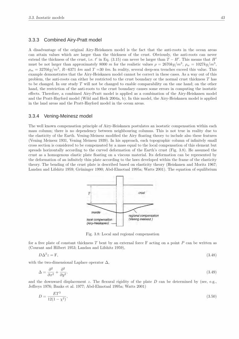
3.3. Isostatic models 43
3.3.3 Combined Airy-Pratt model
A disadvantage of the original Airy-Heiskanen model is the fact that the anti-roots in the ocean areascan attain values which are larger than the thickness of the crust. Obviously, the anti-roots can neverextend the thickness of the crust, i.e. t′ in Eq. (3.15) can never be larger than T −H ′. This means that H ′
must be not larger than approximately 8000 m for the realistic values ρ = 2670kg/m3, ρw = 1027kg
/m3,
ρm = 3270kg/m3, R=6371 km and T =30 km. In reality, several deep-sea trenches exceed this value. This
example demonstrates that the Airy-Heiskanen model cannot be correct in these cases. As a way out of thisproblem, the anti-roots can either be restricted to the crust boundary or the normal crust thickness T hasto be changed. In our study T will not be changed to enable comparability on the one hand; on the otherhand, the restriction of the anti-roots to the crust boundary causes some errors in computing the isostaticeffects. Therefore, a combined Airy-Pratt model is applied as a combination of the Airy-Heiskanen modeland the Pratt-Hayford model (Wild and Heck 2004a, b). In this model, the Airy-Heiskanen model is appliedin the land areas and the Pratt-Hayford model in the ocean areas.
3.3.4 Vening-Meinesz model
The well known compensation principle of Airy-Heiskanen postulates an isostatic compensation within eachmass column; there is no dependency between neighbouring columns. This is not true in reality due tothe elasticity of the Earth. Vening-Meinesz modified the Airy floating theory to include also these features(Vening Meinesz 1931, Vening Meinesz 1939). In his approach, each topographic column of infinitely smallcross section is considered to be compensated by a mass equal to the local compensation of this element butspreads horizontally according to the curved deformation of the Earth’s crust (Fig. 3.8). He assumed thecrust as a homogenous elastic plate floating on a viscous material. Its deformation can be represented bythe deformation of an infinitely thin plate according to the laws developed within the frame of the elasticitytheory. The bending of the crust plate is described based on elasticity theory (Heiskanen and Moritz 1967;Landau and Lifshitz 1959; Grüninger 1990; Abd-Elmotaal 1995a; Watts 2001). The equation of equilibrium
Fig. 3.8: Local and regional compensation
for a free plate of constant thickness T bent by an external force F acting on a point P can be written as(Courant and Hilbert 1953; Landau and Lifshitz 1959),
D∆2z = F, (3.48)
with the two-dimensional Laplace operator ∆,
∆ =∂2
∂x2+
∂2
∂y2. (3.49)
and the downward displacement z. The flexural rigidity of the plate D can be determined by (see, e.g.,Jeffreys 1976; Banks et al. 1977; Abd-Elmotaal 1995a; Watts 2001)
D =ET 3
12(1 − χ2), (3.50)
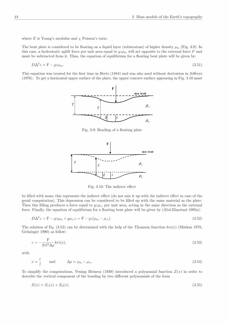
44 3. Mass models of the Earth’s topography
where E is Young’s modulus and χ Poisson’s ratio.
The bent plate is considered to be floating on a liquid layer (substratum) of higher density ρm (Fig. 3.9). Inthis case, a hydrostatic uplift force per unit area equal to gzρm will act opposite to the external force F andmust be subtracted from it. Thus, the equation of equilibrium for a floating bent plate will be given by:
D∆2z = F − gzρm. (3.51)
This equation was treated for the first time in Hertz (1884) and was also used without derivation in Jeffreys(1976). To get a horizontal upper surface of the plate, the upper concave surface appearing in Fig. 3.10 must
sea level
T
T
Z f
crρ
mρ
F
Fig. 3.9: Bending of a floating plate
T
T
Z f
crρ
mρ
sea level
F
Fig. 3.10: The indirect effect
be filled with mass; this represents the indirect effect (do not mix it up with the indirect effect in case of thegeoid computation). This depression can be considered to be filled up with the same material as the plate.Then this filling produces a force equal to gzρcr per unit area, acting in the same direction as the externalforce. Finally, the equation of equilibrium for a floating bent plate will be given by (Abd-Elmotaal 1995a):
D∆2z = F − gzρm + gρcrz = F − gz(ρm − ρcr). (3.52)
The solution of Eq. (3.52) can be determined with the help of the Thomson function kei(x) (Márkus 1978,Grüninger 1990) as follow:
z = − F2πl2∆ρ
kei(x), (3.53)
with
x =r
land ∆ρ = ρm − ρcr. (3.54)
To simplify the computations, Vening Meinesz (1939) introduced a polynomial function Z(x) in order todescribe the vertical component of the bending by two different polynomials of the form
Z(x) = Z1(x) + Z2(x), (3.55)

3.3. Isostatic models 45
with
Z1(x) = f[c1x
6 + c2x4 + c3x
2 + c4]; 0 ≤ x ≤ 2 (3.56)
Z1(x) = f[c5x
4 + c6x2 + c7
]; 0 ≤ x ≤ rmax (3.57)
and
f =mp
8∆ρl2; l = 4
√
D
g∆ρ; x =
r
l, (3.58)
where l is the degree of regionality which describes the mechanical stiffness of the plate using the flexuralrigidity D (Jeffreys 1976; Banks et al. 1977), f is the maximum downward displacement (Vening Meinesz1939, P. 5), rmax is the maximum extension of the regional compensation for one single load/relief (VeningMeinesz 139, p. 713) and mp is the load generated by the topographic masses. In ocean area, mp denotes therelief generated by the ocean water mass deficiencies with the density difference (ρcr − ρw). The coefficient(ci, i = 1, . . ..., 7) can be found, for example, in Heiskanen and Vening Meinesz (1958), Abd-Elmotaal (1991)and Abd-Elmotaal (1995a) as shown in Table 3.1.
Table 3.1: Polynomial coefficients of the bended curve
Coefficients Vening Meinesz Abd-Elmotaal(rmax=2.905l) (rmax=2.914l)
c1 -0.00913 -0.00925c2 0.09906 0.09922c3 -0.35434 -0.34969c4 0.41660 0.40336c5 0.00275 0.00320c6 -0.09234 -0.09748c7 0.58340 0.59664
The difference between the exact solution, given by the elasticity theory, and the approximate solution, givenby Eqs. (3.56) and (3.57), can be neglected in all practical cases (Grüninger 1990, Abd-Elmotaal 1995a).
For the determining the Vening-Meinesz compensation depths, the mass of the point load mp due to a verticalcolumn of topography of density ρcr, height H and infinity small cross sectional area ds, can be written as:
mp = ρcrHds. (3.59)
Thus the bending due to this topographic column will be
Zmp = f(r)ρcrHds. (3.60)
The total bending t due to the entire topographic masses can be given by (Abd-Elmotaal 1995a):
t(x, y) =
∫∫
s
ρcrH(x′, y′)f(r)ds, (3.61)
with
f(r) = z, (3.62)
where ds can be expressed in Cartesian or spherical coordinates as follows:
ds = dxdy, ds = R2 cosϕdϕdλ, (3.63)
and R is the radius of the mean Earth, dϕ and dλ represent the dimensions of the topographic column in thelatitude and the longitude directions, respectively. The total bending t is closely related to the Moho depth
Hm = T + t, (3.64)
where T is the crustal thickness for a topography with zero heights.
46 3. Mass models of the Earth’s topography
3.4 Helmert’s models of condensation
Helmert proposed the condensation method to remove the topographic masses outside the geoid and condensethem onto a surface as a single layer within the masses. One alternative is to condense the topographic masseson a surface parallel to the geoid located at a depth of 21 km below the geoid (Helmert 1884). This depth,corresponding to the difference in the lengths of the equatorial and the minor semi-axes of the Earth ellipsoid,was chosen in order to shift the topographical masses below a sphere situated completely within the geoid.This proposal is the so-called Helmert’s first method of condensation. In a second method, the condensationsurface is the geoid itself. There is a large number of publications referred to Helmerts condensation models,see, e.g., Wichiencharoen (1982); Heck (1992); Martinec et al. (1993); Sjöberg (1994), (1995), (1996a), b;Martinec and Vaníček (1994a, b); Vaníček et al. (1999); Sjöberg and Nahavandchi (1999); Kuhn (2000a), b;Kuhn (2002); Kuhn (2003). Although Helmert’s second method of condensation cannot adequately describethe density distribution within the Earth’s crust, it has been applied for practical determination of the geoid.Its advantage is the very small indirect effect even in case of very high mountains. It is well-known from theanalysis of gravity observations (Kuhn 2000a) that the true gravity field of the Earth contains significantshort wavelengths. These short wavelength constituents are generated by the topographical masses and showapproximately a linear dependency with the topographical heights. Therefore, gravity anomalies computedfrom Helmert’s second method of condensation are as rough as free-air anomalies. This is the reason thatthe downward continuation of the gravity from the surface of the Earth to the geoid in a rough gravityfield may become dubious. Since the short wave-length components cannot be eliminated by the reductionprocedure of Helmert’s second method of condensation, it is obvious that the reduction model implied bythis method cannot work in a satisfaying way in high-resolution applications (Heck 2003). Although someauthors (e.g., Martinec 1995; Kuhn 2000a) have pointed out that the gravity anomalies related to Helmert’ssecond method are strongly correlated with the topographical heights, this model is still widely used in thedetermination of the geoid due to their small indirect effect.
In case of Helmert’s first method of condensation, the reduced gravity is rather smooth (Kuhn 2000a),showing strong similarities to the reduction results by classical isostatic models such as discussed before(Heck 2003). This model approximates the geophysical reality better than Helmert’s second model. With aproper selection of Helmert’s condensation depth D1 the condensation method can be adjusted to a morerealistic topographic-isostatic reality. This modification of Helmert’s condensation method has been proposedby Heck (2003) and can be defined as generalized Helmert method of condensation. In the following the singlelayer density for spherical and planar approximation will be discussed.
Spherical approximation In Helmert’s methods of condensation, the single-layer density k is a functionof the topographical heights. Using the mass conservation principle, the local single-layer density can begiven in spherical approximation as follows (Fig. 4.8):
kR2Cdσ = MT
S , (3.65)
which follows
k =1
R2C
i=l∑
i=0
R+Hi∫
R
(ρi − ρi+1)ξ2dξ, (3.66)
where ρ0, ρl+1 are defined in Eq. (3.2), RC = R for Helmert’s second method of condensation and RC =R−D1 in case of Helmert’s first or generalized method of condensation with Helmert’s condensation depthD1.
After integration and applying a binomial series expansion, the single-layer density can be given by:
k =
l∑
i=0
(ρi − ρi+1)
[(R+H)3i −R3
3R2c
]
=
l∑
i=0
(ρi − ρi+1)
R2c
R3
[(Hi
R
)
+
(Hi
R
)2
+1
3
(Hi
R
)3]
. (3.67)
3.4. Helmert’s models of condensation 47
If the topographic masses have a constant density (one layer with density ρcr), Eq. (3.67) can be simplifiedto
k =ρcrR2c
R3
[(H
R
)
+
(H
R
)2
+1
3
(H
R
)3]
. (3.68)
From the above formulae and from the formulae which will be given in chapter 4 it is shown that therespective formulae for the generalized Helmert’s model of condensation are much simpler than the isostaticmodels (for example the Airy-Heiskanen model). Therefore this model can be considered as a proper methodfor downward continuation and related tasks within the frame of geoid determination (Heck 2003).
The only disadvantage of this generalized method of Helmert is that the indirect effect, primarily due tonon-vanishing components proportional to the topographical height, will be larger than those of Helmert’ssecond method of condensation. It has the same order of magnitude as the indirect effects related to theclassical isostatic models (Kuhn 2002).
Planar approximation In case of the planar approximation, the single layer density is given by using Eq.(3.19) as follows:
dσk =
l∑
i=0
(ρi − ρi+1)Hidσ
k =l∑
i=0
(ρi − ρi+1)Hi,
(3.69)
and for a constant density or the rock equivalent topographic procedures it follows analogously to Eq. (3.24)
k = ρcrHeq. (3.70)

48
4. Computation of the gravitational effects of thetopographic-isostatic masses
The effects of the topographic-isostatic masses can be calculated using analytical, numerical and combinationmethods. The numerical and combination methods are preferable in the case of more than one computationpoint, especially when the goal is the computation of these effects at the points of a regular grid. The lattermay coincide with the outer boundary of the topographic masses as described by the surface relief or maybe located at a given flight altitude above the terrain for airborne gravimetry. The different demands ofthe numerical evaluations depend on the nature of the problem and on the required accuracy level. Theefficiency of the computation methods can be increased by introducing spectral techniques which permit afast evaluation of the respective quantities (Tsoulis and Tziavos 2003).
There are various computation methods which are used for calculating the topographic-isostatic effects:
1. direct integration method,
2. Fast Fourier Transform (FFT),
3. spherical harmonic expansion,
4. spline function,
5. combined method.
The FFT method is restricted first of all to planar applications and has been extensively discussed in the past.In the present applications the focus is on spherical approximations and will, therefore, not be treated here.Details can be found in various publications (see, e.g., Bracewell 1978; Forsberg 1985; Sideris 1985; Schwarzet al. 1990; Parker 1995, 1996; Kirby and Featherstone 1999; Smith 2002; Bracewell 1978; Harrison andDickinson 1989; Li and Sideris 1994). The singularity at the computation point in the numerical calculationof FFT was studied by e.g. Martinec et al. (1996), Kirby and Featherstone (1999), Nagy et al. (2000). Theweak singularities in the terrain correction kernel can be avoided using the procedures derived by Nagyet al. (2000), Tsoulis (1999b) and Klose and Ilk (1993). In the following, the direct integration technique,the spherical harmonic expansion method as well as the space localizing base function technique will bediscussed in detail. Finally, the combinations of these techniques are proposed, including methods whichallow the determination of the topographic-isostatic far-zone effects using also spherical harmonic expansion.
4.1 Direct integration method
In a flat Earth approximation the integration compartments can be represented by rectangular prisms whichis admissible for small areas only. Nevertheless, this approximation is useful for model studies (Nagy et al.2000). The use of spherical models requires extensive computational efforts if tesseroids are used or sphericalharmonic series (Papp and Wang 1996). For instance, in order to resolve 1 x 1 km topography informationin spherical geometry, a spherical harmonic expansion up to degree and order 36 000 would be necessary.Spherical harmonic expansions up to this high degree can not be calculated because of the instability ofthe determination of the associated Legendre functions. Therefore, a spherical harmonic expansion of thetopography may not be selected for a very detailed local modeling.

4.1. Direct integration method 49
4.1.1 Gravitational potential and its derivatives modelled by prisms
4.1.1.1 Effect of the topographic and isostatic masses
The determination of the potential as well as its first and second derivatives by using the integration methodbased on rectangular prisms has been studied by many authors (e.g., Mader 1951; Nagy 1966; Forsberg1984). Formulae for the calculation of the derivatives of the potential up to the third order are given byMader (1951). Here we give only a short review of the gravitational potential, represented by rectangularprisms, as well as of its various derivatives. The gravitational potential of a rectangular prism of homogeneousmass-density ρ is described by Newton’s integral (e.g., Heiskanen and Moritz 1967):
Vt|r=rP= G
∫∫∫
v
ρ(Q)1
l(r, rQ)
∣∣∣∣r=rP
dvQ, (4.1)
where ρ(Q) is the density of the topographic masses or the density contrast of the topographic masses andthe water masses of the oceans. Because of lack of more detailed knowledge, the density of the topographicmasses is assumed to be constant (see, e.g., Vaníček and Kleusberg 1987; Featherstone 1992; Forsberg andSideris 1993; Abd-Elmotaal 1999; Smith and Milbert 1999; Featherstone et al. 2001). However, the realdensity distribution can differ from this value by 10% or more (see, e.g., Martinec 1993; Tziavos el al. 1996;Pagiatakis and Armenakis 1998; Kuhn 2000a, b; Huang et al. 2001).
The point P in Eq.(4.1) is the computation point with the Cartesian coordinates xP , yP , zP and Q (thecenter of the prism) represents the source point with the coordinates x′, y′ and z′ referring to the sameCartesian coordinate system (Fig. 4.1). The quantity l(r, rQ) is the distance between the computation pointand the source point. It is given by the well-known formula,
l(r, rQ)|r=rP
=
√
(x− x′)2
+ (y − y′)2
+ (z − z′)2
∣∣∣∣r=rP
. (4.2)
Insertion of Eq. (4.2) into Eq. (4.1) gives
Vt|r=rP= G
x2∫
x1
y2∫
y1
z2∫
z1
ρ(Q)1
√
(x− x′)2
+ (y − y′)2
+ (z − z′)2
∣∣∣∣∣∣r=rP
dx′dy′dz′. (4.3)
If the density of the prism for simplicity is assumed to be homogeneous and constant (ρcr), the integral of
P(xP,yP,zP)
lPQ
z
x
y
Q(x´,y´,z´)
x
y
z
(x2,y2,z2)
(x1,y1,z1) ∆
∆∆
Fig. 4.1: Notation used for the definition of a prism

50 4. Computation of the gravitational effects of the topographic-isostatic masses
the Eq. (4.3) takes the form (Nagy 1966; Nagy et al. 2000):
V =Gρcr
∣∣∣∣∣
∣∣∣∣
∣∣∣(x− x′)(y − y′) ln((z − z′) + l(r, rQ)) + (x− x′)(z − z′) ln((y − y′) + l(r, rQ)))+
+ (y − y′)(z − z′) ln((x− x′) + l(r, rQ)) − (x− x′)2
2arctan
(y − y′)(z − z′)
(x− x′)l(r, rQ)−
− (y − y′)2
2arctan
(x− x′)(z − z′)
(y − y′)l(r, rQ)− (z − z′)2
2arctan
(x− x′)(y − y′)
(z − z′)l(r, rQ)
∣∣∣∣r=rP
∣∣∣
x2
x1
∣∣∣∣
y2
y1
∣∣∣∣∣
z2
z1
.
(4.4)
The first derivatives of the potential with respected to z are given by (Nagy 1966):
∂V
∂z= −Gρcr
x2∫
x1
y2∫
y1
z2∫
z1
(z − z′)
l(r, rQ)3/2
∣∣∣∣r=rP
dx′dy′dz′, (4.5)
∂V
∂z=Gρcr
∣∣∣∣∣
∣∣∣∣
∣∣∣(x− x′) ln((y − y′) + l(r, rQ)) + (y − y′) ln((x− x′) + l(r, rQ))
−(z − z′) tan [(x− x′)(y − y′)/((z − z′)l(r, rQ))]∣∣∣
x2
x1
∣∣∣∣
y2
y1
∣∣∣∣∣
z2
z1
.
(4.6)
The other two partial derivatives of the potential with respect to x, y can be obtained from Eq. (4.6) bycyclic permutation
∂V
∂x=Gρcr
∣∣∣∣∣
∣∣∣∣
∣∣∣(y − y′) ln((z − z′) + l(r, rQ)) + (z − z′) ln((y − y′) + l(r, rQ)))−
−(x− x′) tan [(y − y′)(z − z′)/((x− x′)l(r, rQ))]∣∣∣
x2
x1
∣∣∣∣
y2
y1
∣∣∣∣∣
z2
z1
,
(4.7)
∂V
∂y=Gρcr
∣∣∣∣∣
∣∣∣∣
∣∣∣(z − z′) ln((x− x′) + l(r, rQ)) + (x− x′) ln((y − y′) + l(r, rQ)))−
−(y − y′) tan [(x− x′)(z − z′)/ ((y − y′)l(r, rQ))]∣∣∣
x2
x1
∣∣∣∣
y2
y1
∣∣∣∣∣
z2
z1
.
(4.8)
The second derivatives of the potential are given by (ibid.)
∂2V
∂x2= Gρcr
∣∣∣∣∣
∣∣∣∣
∣∣∣− arctan
(y − y′)(z − z′)
(x− x′)l(r, rQ)
∣∣∣
x2
x1
∣∣∣∣
y2
y1
∣∣∣∣∣
z2
z1
, (4.9)
∂2V
∂y2= Gρcr
∣∣∣∣∣
∣∣∣∣
∣∣∣− arctan
(x− x′)(z − z′)
(y − y′)l(r, rQ)
∣∣∣
x2
x1
∣∣∣∣
y2
y1
∣∣∣∣∣
z2
z1
, (4.10)
∂2V
∂z2= Gρcr
∣∣∣∣∣
∣∣∣∣
∣∣∣− arctan
(x− x′)(y − y′)
(z − z′)l(r, rQ)
∣∣∣
x2
x1
∣∣∣∣
y2
y1
∣∣∣∣∣
z2
z1
, (4.11)
∂2V
∂x∂y= Gρcr
∣∣∣∣∣
∣∣∣∣
∣∣∣ln((z − z′) + l(r, rQ))
∣∣∣
x2
x1
∣∣∣∣
y2
y1
∣∣∣∣∣
z2
z1
, (4.12)
∂2V
∂x∂z= Gρcr
∣∣∣∣∣
∣∣∣∣
∣∣∣ln((y − y′) + l(r, rQ))
∣∣∣
x2
x1
∣∣∣∣
y2
y1
∣∣∣∣∣
z2
z1
, (4.13)

4.1. Direct integration method 51
∂2V
∂y∂z= Gρcr
∣∣∣∣∣
∣∣∣∣
∣∣∣ln((x− x′) + l(r, rQ))
∣∣∣
x2
x1
∣∣∣∣
y2
y1
∣∣∣∣∣
z2
z1
. (4.14)
From Eqs. (4.4) to (4.14), it is easy to realize that these formulae show singularities for special locations of P(e.g., if P coincides with a prism’s corner or is situated on an edge of the prism); the respective limit valueshave been derived by Nagy et al. (2000, 2002). The above relations can be used for calculating the potentialand its first and second derivatives of the topographic masses on or above the surface of the Earth. Since theprism matches the concept of the DTM, the TC software (Forsberg 1984) for prismatic topographic elementssituated in an intermediate zone can be used after modifying it for calculating different topographic-isostaticmodels.
Due to the decrease of the gravitational effects with increasing distance, the complex formula (4.4) can besubstituted by a simpler one for prisms which are located at a large distance from the computation point.This simpler formula can be derived based on a Taylor expansion of the integration kernel in Eq. (4.1). TheTaylor expansion is fixed at the geometrical centre of the prism. The gravitational potential of the rectangularprism neglecting terms of order four and higher is given by MacMillan’s (1930) formula (also see Anderson1976; Forsberg 1984; Heck and Seitz 2006):
V = Gρcr∆x∆y∆z
[
1
l0+
3 (x0 − x)2 − l20
24l50∆x2 +
3 (y0 − y)2 − l20
24l50∆y2 +
3 (z0 − z)2 − l20
24l50∆z2 + ....
]
, (4.15)
where
xo = (x1 + x2)/2,
yo = (y1 + y2)/2,
zo = (z1 + z2)/2.
(4.16)
and l0 denotes the Euclidean distance between the computation point P and the geometrical center (x0, y0, z0)of the computation prism with ∆x = x2 − x1, ∆y = y2 − y1 and ∆z = z2 − z1. The first and higher orderderivatives of the potential can be simply found by differentiation of Eq. (4.15) with respect to x, y andz. Near the computation point (Eqs. 4.4 to 4.14), the flat-topped approximation of the topographic prismis assumed. This approximation produces some errors for the computation of the gravitational functions. Abetter approximation can be supplied by a prism topped by an inclined plane (Koch 1965) or by a bilinearsurface (Smith 2000; Tsoulis et al. 2003). This procedure can be transformed to polyhedral bodies which caneasily be determined by numerical methods (Talwani and Ewing 1960; Paul 1974; Petrović 1996).
For prisms which are far from the computation point, the curvature of the Earth must be taken into account.These prisms are inclined with respect to the local vertical and shifted with respect to the horizontal planeat the computation point, due to the (approximate) sphericity of the Earth. These effects have to be takeninto account for distant prismatic elements (Grüninger 1990; Kuhn 2000a; Smith 2000, 2002). Also, dueto the curvature of the Earth, the topocentric Cartesian coordinate systems, according to the direction ofthe vertical at the computation point and the edges of the prismatic topographic element, are not parallel.The transformation between the two systems is visualized in Fig.4.2 where (X,Y, Z) denote the Cartesiancoordinates related to a global terrestrial reference frame and (x, y, z) and (x∗, y∗, z∗) the local Cartesiancoordinates related to the edge system of the prism and the local vertical reference frame at the computationpoint P , respectively. The transformation of the first derivatives of the potential known in the edge systeminto the local coordinate system at P is given by the respective basis transformation with respect to theglobal equatorial system (Heck and Seitz 2006). The direction of the plumbline at the computation point isdefined by the geodetic latitude ϕ and the geodetic longitude λ of the point P . The direction of the z-axisof the edge system is defined by ϕ′ and λ′. The relations between the orthonormal base vectors are given by(Grüninger 1990; Kuhn 2000a; Heck and Seitz 2006)
(ex, ey, ez)T
= P1 · R2
(π
2− ϕ′
)
· R3 (λ′) · (eX, eY, eZ)T, (4.17)
(e∗x, e
∗
y, e∗
z
)T= P1 · R2
(π
2− ϕ
)
· R3 (λ) · (eX, eY, eZ)T, (4.18)

52 4. Computation of the gravitational effects of the topographic-isostatic masses
x
y
z
P´
X
Y
Z
ϕλ
λ′
z*
y*
x*
(x1,y1,z1)
x
y
P(x2,y2,z2)
ϕ′
∆
∆
∆z
Fig. 4.2: Transformation between the edge system of the prism and the local vertical system at the compu-tation point
where R2 and R3 are the rotation matrices for rotations about the y- and z-axis, respectively, while thereflection matrix P1 has to be introduced for the transition between the right-handed global system andthe left-handed local system. In numerical applications, the geodetic latitudes ϕ, ϕ′ may be replaced by thegeocentric latitudes. From Eqs. (4.17) and (4.18) the formula for the transformation between the edge systemof the prism and the local vertical system at the computation point is given by (Kuhn 2000a):
(v∗x, v∗
y , v∗
z)T = R(ϕ, λ, ϕ′, λ′) · (vx, vy, vz)T , (4.19)
where (v∗x, v∗
y , v∗
z) and (vx, vy, vz) are the first derivatives of the potential in the edge system and in the localvertical system at P , respectively. The transformation matrix R(ϕ, λ, ϕ′, λ′) is given by (ibid.)
R(ϕ, λ, ϕ′, λ′) =
s1s′
1(c2c′
2 + s2s′
2) + c1c′
1 s1(−c2s′2 − s2c′
2) −s1c′1(c2c′2 + s2s′
2) + c1c′
1
s′1(s2c′
2 + c2s′
2) s2s′
2 + c2c′
2 c′1(−s2c′2 + c2s′
2)−c1s′1(c2c′2 + s2s
′
2) + s1c′
1 c1(−c2s′2 + s2c′
2) c1c′
1(c2c′
2 + s2s′
2) + s1s′
1
(4.20)
with
s1 = sinϕ, s2 = sinλ, c1 = cosϕ, c2 = cosλ,s′1 = sinϕ′, s′2 = sinλ′, c′1 = cosϕ′, c′2 = cosλ′.
(4.21)
This transformation is carried out for every single prism situated at a large distance from the computationpoint P . Also, the second derivatives of the potential can be transformed using the same transformationmatrix given in Eq. (4.20).
The dimensions of the prism have to be derived from the dimensions of a tesseroid. These dimensions canbe determined based on the mass conservation as follows:
mtesseroid = mprism, (4.22)
which follows
∆z = ∆r,
∆x = R∆ϕ,
∆y = R cosϕ∆λ.
(4.23)

4.1. Direct integration method 53
For calculating the effects of the topographic masses, the height of the prismatic element is taken to be equalto the orthometric height of the topography of this element with ρ equals the density of the masses in caseof land areas. In case of ocean regions the density is taken to be
ρ(xQ, yQ, zQ) = ρw − ρcr, (4.24)
where ρcr is the density of the crust and ρw the density of the water. For calculating the effects of theisostatic masses in case of Airy-Heiskanen and Vening Meinesz models, the height of the prismatic elementis taken to be equal to the roots or antiroots of the isostatic masses with density contrast ∆ρ = ρm − ρcr.In case of the Pratt-Hayford model, the height of the prismatic element is taken to be equal to the heightof the orthometric height of the topography in addition to the Pratt-Hayford compensation depth with thedensity contrast as determined in chapter 3 for land and ocean areas.
4.1.1.2 Effect of the condensation masses
For calculating the effect of the condensation masses in the case of Helmert’s methods of condensation usingthe prism integration method, Eq. (4.1) will be transformed to the following equation (Smith et al. 2001):
Vc|r=rP= G
∫∫
σ
kQl∗(r, rQ)
∣∣∣∣r=rP
dx′dy′, (4.25)
with the surface element dσ =dxQdyQ and the single layer density kQ, which depends on the height anddensity of the topography (see chapter 3). If the density of the prism is taken to be constant (ρcr), thepotential, the first and the second derivatives can be determined as follows (see Fig. 4.3):
z
x
y
x
y
z
(x2,y2,z2)
(x1,y1,z1)
Q(x´,y´,z*)
P(x,y,z)
l*
∆
∆
∆
Fig. 4.3: Notation used for the definition of a condensed prism
Vc|r=rP=Gρcr∆z
∣∣∣∣
∣∣∣(x− x′) ln((y − y′) + l∗(r, rQ)) + (y − y′) ln((x− x′) + l∗(r, rQ))−
− z arctan [(x− x′)(y − y′)/((z − z∗)l∗(r, rQ))]|r=rP
∣∣∣
x2
x1
∣∣∣∣
y2
y1
,
(4.26)
∂Vc∂z
= Gρcr∆z
∣∣∣∣
∣∣∣− arctan [(x− x′)(y − y′)/((z − z∗)l∗(r, rQ))]
∣∣∣
x2
x1
∣∣∣∣
y2
y1
, (4.27)
∂Vc∂x
= Gρcr∆z
∣∣∣∣
∣∣∣ln((y − y′) + l∗(r, rQ))
∣∣∣
x2
x1
∣∣∣∣∣
y2
y1
, (4.28)
∂Vc∂y
= Gρcr∆z
∣∣∣∣
∣∣∣ln((x− x′) + l∗(r, rQ))
∣∣∣
x2
x1
∣∣∣∣
y2
y1
, (4.29)

54 4. Computation of the gravitational effects of the topographic-isostatic masses
∂2Vc∂z2
= Gρcr∆z
∣∣∣∣
∣∣∣(x− x′)(y − y′)
l∗(r, rQ)
(1
(x− x′)2 + (z − z∗)2+
1
(y − y′)2 + (z − z∗)2
)∣∣∣
x2
x′=x1
∣∣∣∣
y2
y′=y1
, (4.30)
∂2Vc∂x2
= Gρcr∆z
∣∣∣∣
∣∣∣
(x− x′)
l∗(r, rQ)((y − y′) + l∗(r, rQ))
∣∣∣
x2
x1
∣∣∣∣
y2
y1
, (4.31)
∂2Vc∂y2
= Gρcr∆z
∣∣∣∣
∣∣∣
(y − y′)
l∗(r, rQ)((x− x′) + l∗(r, rQ))
∣∣∣
x2
x1
∣∣∣∣
y2
y1
, (4.32)
∂2Vc∂x∂y
= Gρcr∆z
∣∣∣∣
∣∣∣
1
l∗(r, rQ)
∣∣∣
x2
x1
∣∣∣∣
y2
y1
, (4.33)
∂2Vc∂x∂z
= Gρcr∆z
∣∣∣∣
∣∣∣
(z − z∗)
l∗(r, rQ)((y − y′) + l∗(r, rQ))
∣∣∣
x2
x1
∣∣∣∣
y2
y1
, (4.34)
∂2Vc∂y∂z
= Gρcr∆z
∣∣∣∣
∣∣∣
(z − z∗)
l∗(r, rQ)((x− x′) + l∗(r, rQ))
∣∣∣
x2
x1
∣∣∣∣
y2
y1
, (4.35)
where
l∗(r, rQ) =((x− x′)2 + (y − y′)2 + (z − z∗)2
)1/2. (4.36)
In our case ∆z = z2 − z1 is equal to the orthometric height of the prismatic element and z∗ the verticalcoordinate of the geometrical center of the condensed integration element.
4.1.2 Gravitational potential and its derivatives modelled by tesseroids (using the analy-tic vertical integration)
Taking the curvature of the Earth into account, a much better level of approximation in the calculation ofthe topographic mass effects is obtained. In this case the geoid can be modelled by a sphere of radius R,coinciding with the mean radius of the Earth. There are two principal possibilities: a representation of thetopography by any spherical discretisation and a subsequent integration (Smith et al. 2001; Tenzer et al.2003; Heck 2003) or a representation of the topography by a spherical harmonic expansion (see, e.g., Sünkel1985, 1986; Rummel et al. 1988; Tsoulis 1999a, 2001). In the case of the direct integration method, the weaksingularities are solved numerically by separating the topographic masses in spherical approximation in twoterms: the spherical Bouguer shell and a spherical terrain correction (see, e.g., Novák et al. 2001; Vaníček etal. 2001; Heck 2003). The effects of the spherical shell on the potential and its first and second derivativesare studied in many previous investigations such as Wichiencharoen (1982), Blakely (1995), Vaníček et al.(2001), Tenzer et al. (2003), Vajda et al. (2004a), (2004b) and Vaníček et al. (2004).
4.1.2.1 Effect of the topographic masses
The potential of the topographic masses between the topographic surface S and the sphere of radius R atthe computation point P is given by Newton’s integral in spherical coordinates as follows (Fig. 4.4):
Vt|r=rP= G
∫∫
σ
rQ∫
R
ρ(Q)ξ2
l
∣∣∣∣r=rP
dξ
dσ, (4.37)
with
l :=√
r2 + ξ2 − 2rξ cosψ, (4.38)
the density of the topography ρ(Q), rQ = R + HQ, and the surface element in spherical coordinatesdσ = cosϕQdϕQdλQ. ρ(Q) is the density of the spherical integration element; it reads in case of the ocean

4.1. Direct integration method 55
area ρ(Q) = ρcr − ρw. The geocentric angle ψ is the spherical distance between the radius vectors of thecomputation point rP (r, ϕ, λ) and the integration point rQ(rQ, ϕQ, λQ):
cosψ = sinϕ sinϕQ + cosϕ cosϕQ cos(λQ − λ), (4.39)
where ϕ and λ are the geodetic latitude and longitude of the computation point, respectively. Additionalquantities are shown in Fig. 4.4. If the column of topography consists of several layers with different densities(Fig. 3.2, left), the potential of the topographic masses is given by:
Vt|r=rP= G
∫∫
σ
R+Hi∫
R
i=l∑
i=0
(ρi − ρi+1)ξ2
l
∣∣∣∣r=rP
dξ
dσ, (4.40)
where ρ0, ρl+1 are defined in Eq. (3.2). If the rock equivalent representation is used, Eq. (4.37) is transformedto
Vt|r=rP= Gρcr
∫∫
σ
rQ∫
R
ξ2
l
∣∣∣∣r=rP
dξ
dσ. (4.41)
The inner integral of Eq. (4.37) can be evaluated by using (Gradshteyn and Ryzhik 1980):
Vt|r=rP=
1
2Gρcr
∫∫
σ
[F0(r, ψ, ξ)|r=rP
]rQ
ξ=Rdσ, (4.42)
with
F0(r, ψ, ξ) = (ξ + 3r cosψ)l(r, ψ, ξ) + r2(3cos2ψ − 1) ln(l(r, ψ, ξ) + ξ − r cosψ) (4.43)
and rP = (R + HP , ϕ, λ). The integration interval in Eq. (4.42) can be separated into two parts, (R, rP ′)and (rp′ , rQ). The quantity rP ′ = R+Hp′ denotes the geocentric radius of the surface point P ′ ∈ S whichis located under the computation point P (Fig. 4.4). Then the integral of Eq. (4.3) can be given by (Heck2003):
Vt|r=rP=
2πGρcrrP
2
3(r3P ′ −R3) ∀rP ≥ rP ′
rP (r2P ′ −R2) ∀rP ≤ rP ′
+
1
2Gρcr
∫∫
σ
[rQ l
′ − rP ′ l+
+3rP cosψ(l′ − l) + r2P (3 cos2 ψ − 1) ln
∣∣∣∣
l′ + rQ − rP cosψ
l + rP ′ − rP cosψ
∣∣∣∣
]
dσ,
(4.44)
with the Euclidean distances as shown in Fig. 4.4 and defined by:
l :=√
r2P + r2P ′ − 2rP rP ′ cosψ, (4.45)
l′ :=√
r2P + r2Q − 2rP rQcosψ. (4.46)
The first term in Eq. (4.44) is due to the mass of a homogenous spherical shell of thickness HP ′ = rP ′ − Racting on the gravitational potential at the computation point P . Two cases have to be distinguished: thepoint is located either on or outside the topography of the Earth (rP ≥ rP ′) or the point is located belowor on the geoid (rP ≤ rP ′). The integral term in Eq. (4.44) denotes the influence of the varying terraindue to rQ 6= rP ′(terrain correction). The first case (rP ≥ rP ′) will be used to determine the effect of thetopographic-isostatic masses at the surface of the Earth or outside at aeroplane or satellite altitude. Thesecond case of Eq. (4.44) is necessary only for the calculation of the primary indirect topographical effect onthe geoidal height.
The first and second derivatives of the potential of the topographic masses are determined in a tangentialcoordinate system. This tangential coordinate system is defined with the x-axis oriented to north, the z-axis

56 4. Computation of the gravitational effects of the topographic-isostatic masses
coinciding with the radius vector and the y-axis oriented to east, completing a left-hand-system (see Fig.4.5). The first derivatives of the potential of the topographic masses with respect to z can be calculatedusing the following formula (Novák et al. 2001):
∂Vt∂z
=∂Vt∂r
, (4.47)
∂Vt∂r
∣∣∣∣r=rP
= − 4πGρcr3r2
(r3p′ −R3)
∣∣∣∣r=rP
+Gρcr
∫∫
σ
[F1(r, ψ, ξ|r=rP
)]rQ
ξ=rP ′
dσ, (4.48)
F1(r, ψ, ξ) =([
(ξ2 + 3r2) cosψ + ξr(1 − 6 cos2 ψ)]/l(r, ψ, ξ)+
+ r(3 cos2 ψ − 1) ln |ξ − r cosψ + l(r, ψ, ξ)|) .(4.49)
The first derivative of the potential of the topographic masses with respect to x can be calculated as follows(Tscherning 1976):
∂Vt∂x
∣∣∣∣r=rP
=1
r
∂Vt∂ϕ
∣∣∣∣r=rP
=1
r
∂ψ
∂ϕ
∂Vt∂ψ
∣∣∣∣r=rP
, (4.50)
It follows from Eq. (4.37) with Eq. (4.38) according to Fig. 4.5,
∂Vt∂ψ
∣∣∣∣r=rP
= Gρcr
∫∫
σ
[
∂F0
∂ψ
∣∣∣∣r=rP
]rQ
R
dσ, (4.51)
geoid
PH
P¢r
P
P¢
Qr
Qr
ξ
Q
Q¢
QH
Q
Pr ¢
0P
0Pr
Pr
PH ¢
l
l
l¢
l
l¢
Wr
r
r
r
P¢
yR
P¢
PH ¢
s
geoid
Earth surface S
shell for point
computation point
integration point
integration point
shell for point
cr
cr
cr
Fig. 4.4: Geometry of the topography in spherical approximation

4.1. Direct integration method 57
PH
P
0Q
0P
y
R
Xe
Ye
Ze
ze
xe
xe
ye
ye
ze
l
Ql
j
Qj
Ql l-
Qa
computation point
integration point
Fig. 4.5: Local coordinate system
with
∂F0
∂ψ
∣∣∣∣r=rP
=: F2(r, ψ, ξ)|r=rP, (4.52)
and according to Heiskanen and Moritz (1967),
∂ψ
∂ϕ= − cosαQ, (4.53)
with the spherical azimuth αQ as given by e.g. Heiskanen and Moritz (1967, Eq. 2-212):
tanαQ =cosϕQ sin(λQ − λ)
sinϕQ cosϕ− cosϕQ sinϕ cos (λQ − λ). (4.54)
The integration interval in Eq. (4.51) is again separated into two parts, (R, rP ′) and (rp′ , rQ). The first partrepresents the effect of the spherical Bouguer shell and is zero for the first derivatives in x and y directions.Then the second part can be given by:
∂Vt∂ψ
∣∣∣∣r=rP
= Gρcr
∫∫
σ
[F2(r, ψ, ξ)|r=rP
]rQ
rP ′
dσ, (4.55)
with
F2(r, ψ, ξ) =[−(rξ2 sinψ − r2ξ cosψ(5 − 6 cos2 ψ)/ sinψ + r3(2 − 3 cos2 ψ)/ sinψ
)/
− l(r, ψ, ξ) −(r2(3/2 sin 2ψ) ln |ξ − r cosψ + l(r, ψ, ξ)|
)].
(4.56)
The first derivative of the potential of the topographic masses with respect to y can be determined analogouslyto Eq. (4.50) resulting in the formula,
∂Vt∂y
∣∣∣∣r=rP
=1
r cosϕ
∂Vt∂λ
∣∣∣∣r=rP
=1
r cosϕ
∂ψ
∂λ
∂Vt∂ψ
∣∣∣∣r=rP
, (4.57)

58 4. Computation of the gravitational effects of the topographic-isostatic masses
where ∂Vt/∂ψ|r=rPis given by Eq. (4.55) and
∂ψ
∂λ= − cosϕ sinαQ, (4.58)
based on the Eq. (4.39) and Eq. (4.54). Eqs. (4.48), (4.50) and (4.57) can be used to study the effects ofthe topographic masses on Satellite-to-Satellite Tracking (SST) observations as shown in Makhloof and Ilk(2004).
The second derivatives of the potential of the topographic masses are important for airborne or SatelliteGravity Gradiometry. It holds for the radial component, starting from Eq. (4.48):
∂2Vt∂z2
∣∣∣∣r=rP
=∂2Vt∂r2
∣∣∣∣r=rP
, (4.59)
with
∂2Vt∂r2
∣∣∣∣r=rP
=8πGρcr
3r3(r3P ′ −R3)
∣∣∣∣r=rP
+Gρcr
∫∫
σ
[
∂F1(r, ψ, ξ)
∂r
∣∣∣∣r=rP
]rQ
ξ=rP ′
dσ, (4.60)
and
∂F1(r, ψ, ξ)
∂r
∣∣∣∣r=rP
=: F3(r, ψ, ξ)|r=rP, (4.61)
where F3(r, ψ, ξ) can be given after some algebraic operations by:
F3(r, ψ, ξ) =([
(ξ cosψ − r)((ξ2 + 3r2) cosψ + rξ(1 − 6 cos2 ψ)
)]l−3(r, ψ, ξ)
+ (3 cos2 ψ − 1) ln |ξ − r cosψ + l(r, ψ, ξ)|++[2ξ + 6r cosψ − 9ξ cos2 ψ
]l−1(r, ψ, ξ)
).
(4.62)
The second derivative of the potential of the topographic masses with respect to x can be given by therelation (Tscherning 1976),
∂2Vt∂x2
∣∣∣∣r=rP
=1
r
∂Vt∂r
∣∣∣∣r=rP
+1
r2∂2Vt∂ϕ2
∣∣∣∣r=rP
. (4.63)
The first term is given by Eq. (4.48) and the second term can be derived starting from Eq. (4.50):
1
r2∂2Vt∂ϕ2
∣∣∣∣r=rP
=1
r2
[
∂2Vt∂ψ2
(∂ψ
∂ϕ
)2
+∂Vt∂ψ
∂2ψ
∂ϕ2
]∣∣∣∣∣r=rP
, (4.64)
with
∂2ψ
∂ϕ2= sin2 αQ cotψ, (4.65)
by considering Eqs. (4.53), (4.39) and (4.54). The term
∂2Vt∂ψ2
∣∣∣∣r=rP
= Gρcr
∫∫
σ
[
F2(r, ψ, ξ)
∂ψ
∣∣∣∣r=rP
]rQ
rP ′
dσ (4.66)
follows from Eq. (4.51) with Eq. (4.52) with the relation
F2(r, ψ, ξ)
∂ψ
∣∣∣∣r=rP
=: F4(r, ψ, ξ)|r=rP, (4.67)

4.1. Direct integration method 59
where F4(r, ψ, ξ) can be expressed after some algebraic operations by:
F4(r, ψ, ξ) = −[3r2(cos 2ψ) ln |ξ − r cosψ + l(r, ψ, ξ)|
]+
+[rξ(rξ2 sin2 ψ− r2ξ cosψ(5 − 6 cos2 ψ) + r3(2 − 3 cos2 ψ)
)/l3(r, ψ, ξ)
]+
+[(−rξ2 cosψ + 15r2ξ cos2 ψ − r2ξ(5 − 6 cos2 ψ)/ sin2 ψ −
−9r3 cosψ + r3 cosψ(2 − 3 cos2 ψ)/ sin2 ψ)/l(r, ψ, ξ)
].
(4.68)
The second derivative of the potential of the topographic masses with respect to y, (Vt)yy, reads as follows(Tscherning 1976):
∂2Vt∂y2
∣∣∣∣r=rP
=1
r
∂Vt∂r
∣∣∣∣r=rP
+1
r2 cos2 ϕ
∂2Vt∂λ2
∣∣∣∣r=rP
− tanϕ
r2∂Vt∂ϕ
∣∣∣∣r=rP
. (4.69)
The first term of Eq. (4.69) coincides with the first term of Eq. (4.63) and is given by Eq. (4.48) correspondingto Eq. (4.50) and the second term can be calculated starting from
1
r2 cos2 ϕ
∂2Vt∂λ2
∣∣∣∣r=rP
=1
r2 cos2 ϕ
[
∂2Vt∂ψ2
(∂ψ
∂λ
)2
+∂Vt∂ψ
∂2ψ
∂λ2
]∣∣∣∣∣r=rP
, (4.70)
with the first derivative as given in Eq. (4.58) and the second derivative
∂2ψ
∂λ2= cos2 αQ cos2 φ cotψ − 1
2sin 2φ cosαQ, (4.71)
again based on Eq. (4.39) and Eq. (4.54).
The derivatives ∂Vt/∂ψ and ∂2Vt/∂ψ2 are given by Eq. (4.55) and Eq. (4.66), respectively. The mixed second
derivatives (Vt)xz and (Vt)yz read according to Tscherning (1976):
∂2Vt∂x∂z
∣∣∣∣r=rP
= − 1
r2∂Vt∂ϕ
∣∣∣∣r=rP
+1
r
∂2Vt∂ϕ∂r
∣∣∣∣r=rP
, (4.72)
∂2Vt∂y∂z
∣∣∣∣r=rP
= − 1
r2 cosϕ
∂Vt∂λ
∣∣∣∣r=rP
+1
r cosϕ
∂2Vt∂r∂λ
∣∣∣∣r=rP
. (4.73)
The first term of Eq. (4.72) is given by Eq. (4.50) and the second term can be determined from the followingformula:
1
r
∂2Vt∂ϕ∂r
∣∣∣∣r=rP
=1
r
∂2Vt∂r∂ψ
∣∣∣∣r=rP
∂ψ
∂ϕ= −1
r
∂2Vt∂r∂ψ
cosαQ
∣∣∣∣r=rP
, (4.74)
with
∂2Vt∂r∂ψ
∣∣∣∣r=rP
= Gρcr
∫∫
σ
[
∂F2(r, ψ, ξ)
∂r
∣∣∣∣r=rP
]rQ
rP ′
dσ, (4.75)
where
∂F2(r, ψ, ξ)
∂r
∣∣∣∣r=rP
=: F5(r, ψ, ξ)|r=rP. (4.76)
F5(r, ψ, ξ) can be derived from Eq. (4.56) by differentiating with respect to r and after some rearrangements:
F5(r, ψ, ξ) = [−rξ sinψ(cos ψ(ξ2 + 3r2) + rξ(1 − 6 cos2 ψ))l−3(r, ψ, ξ)+
+(6rξ sin 2ψ − sinψ(ξ2 + 3r2)
)l−1(r, ψ, ξ)−
− 3r sin 2ψ ln |ξ + l(r, ψ, ξ) − r cosψ|
+r sinψ(l(r, ψ, ξ) + ξ)
l(r, ψ, ξ)(l(r, ψ, ξ) + ξ − r cosψ)r(3 cos2 ψ − 1)
].
(4.77)

60 4. Computation of the gravitational effects of the topographic-isostatic masses
The first term of the mixed derivatives (Vt)yz (see Eq. 4.73) reads as shown in Eq. (4.57) and the secondterm can be determined as follows:
1
r cosϕ
∂2Vt∂r∂λ
∣∣∣∣r=rP
=1
r cosϕ
∂2V
∂r∂ψ
∣∣∣∣r=rP
∂ψ
∂λ= −1
r
∂2Vt∂r∂ψ
sinαQ
∣∣∣∣r=rP
, (4.78)
with ∂2Vt/∂r∂ψ∣∣r=rP
as given by Eq. (4.75).
Finally, the mixed second derivative in (Vt)xy can be derived based on the formula (Tscherning 1976):
∂2Vt∂x∂y
∣∣∣∣r=rP
= − tanϕ
r2 cosϕ
∂Vt∂λ
∣∣∣∣r=rP
+1
r2 cosϕ
∂2Vt∂ϕ∂λ
∣∣∣∣r=rP
= − tanϕ
r
∂Vt∂y
∣∣∣∣r=rP
+1
r2 cosϕ
∂Vt∂ϕ∂λ
∣∣∣∣r=rP
.
(4.79)
The first term at the right hand side of Eq. (4.79) is given by Eq. (4.57) and the second term reads:
1
r2 cosϕ
∂2Vt∂ϕ∂λ
∣∣∣∣r=rP
=1
r2P cosϕ
[
∂2Vt∂ψ2
∂ψ
∂ϕ
∂ψ
∂λ
∣∣∣∣r=rP
+∂2ψ
∂ϕ∂λ
∂Vt∂ψ
∣∣∣∣r=rP
]
, (4.80)
where
∂2ψ
∂ϕ∂λ= sinαQ(sinϕ− cosϕ cosαQ cotψ). (4.81)
∂Vt/∂ψ as well as ∂2Vt/∂ψ2 can be determined using Eq. (4.55) and Eq. (4.66), respectively.
4.1.2.2 Effect of the isostatic masses
In the previous section, the effect of the uncompensated topographic masses has been studied. In the following,the contributions of the isostatic compensating masses due to different models will be investigated.
Airy-Heiskanen model The topography of height H = 0 corresponds to the normal thickness T of theEarth’s crust with the density equal to the density of the topography ρ. The higher the mountains are, thedeeper they sink (see Fig. 4.6). Thus the thickness of a root column under a mountain column with heightH can be determined by the formulae as given in chapter 3. The potential of the isostatic masses at thecomputation point P can be determined in the same way as the potential of the topographic masses, see Eq.4.37
VI |r=rP= G∆ρ
∫∫
σ
R−T∫
R−T−tQ
ξ2
l
∣∣∣∣r=rP
dξ
dσ, (4.82)
with the spherical surface element dσ of a sphere with radius R and the integration variable ξ and l due to
l :=√
r2 + ξ2 − 2rξ cosψ. (4.83)
The integration interval (R− T − tQ, R− T ) can be decomposed again into two parts, the terrain correction(R− T − tQ, R− T − tP ′) and the shell of thickness (R− T − tP ′ , R− T ) where tP ′ is the thickness of theroot or the anti-root under the computation point P or P ′, respectively (Fig. 4.6). Then the formula forthe potential of the isostatic compensation masses can be given by a formula similar to Eq. (4.42) with Eq.(4.43):
VI |r=rP=
4πG∆ρ
3rP
[(R− T )3 − (R− T − tP )3
]+G∆ρ
2
∫∫
σ
[F0(r, ψ, ξ)|r=rP
]R−T−tQ
R−T−tPdσ, (4.84)

4.1. Direct integration method 61
s
Earth surface S
integration point
computation point
H
Qr
Q
geoid
Pr
H ¢
t ¢
Wr
r
mr
R
P¢
TcQ
cP¢
t
mr r rD = -
P
cP¢
P
P¢QQ
HPH ¢
P¢ Pr
cQ
cP¢
Pt
Qt
H
t
geoid s
computation point
shell for point
shell for point
Earth surface S
Fig. 4.6: Spherical Airy-Heiskanen topographic-isostatic model
where ∆ρ = ρm − ρcr is the difference between the density of the mantle and the density of the isostaticcompensation masses and F0(r, ψ, ξ) is given by Eq. (4.43). The first term of Eq. (4.84) represents the effectof the spherical Bouguer shell of the compensating masses for point P ′
c.
The first and second derivatives of the potential of the isostatic compensation masses necessary for airbornevector gravimetry and gradiometry at aeroplane or satellite altitude can be determined using the sameformulae as applied for the determination of the effects of the topographic masses. Only the integrationlimits have to be selected properly as illustrated in Fig. 4.6. The radial derivative (VI)z (z -direction, seeFig. 4.5) reads
∂VI∂z
∣∣∣∣r=rP
= −4πG∆ρ
3r2P
[(R− T )3 − (R− T − tP )3
]+G∆ρ
∫∫
σ
[F1(r, ψ, ξ)|r=rP
]R−T−tQ
R−T−tPdσ, (4.85)
where F1(r, ψ, ξ) is given by Eq. (4.49). The effects of the compensating masses on the other components ofthe first and second derivatives can be determined analogously.
The combined effect of the topographic-isostatic masses on the different gravity functionals is the differencebetween the effect of the topographic masses and the effect of the isostatic compensation masses. It readse.g.,
VTI |r=rP= Vt|r=rP
− VI |r=rP. (4.86)
In the previous formulae in spherical approximation the topographic effects are calculated by setting Heq forH. If the density is laterally variable, the thickness of the rock equivalent heights Heq can be determined bythe condition that the mass density of an equivalent rock layer is equal to the mass density of the constantcrust (see chapter 3).
All the equations derived for the Airy-Heiskanen model can be used also for the Vening-Meinesz model withthe only difference that the roots and anti-roots are determined according to the equations given in chapter3 (see, e.g., Abd-Elmotaal 1995a; Vening Meinesz 1939, 1941).
Pratt-Hayford model In case of the Pratt-Hayford model the effect of the topographic masses is calcu-lated in two parts: one for the land areas and the other for the ocean areas. The same has to be done for the
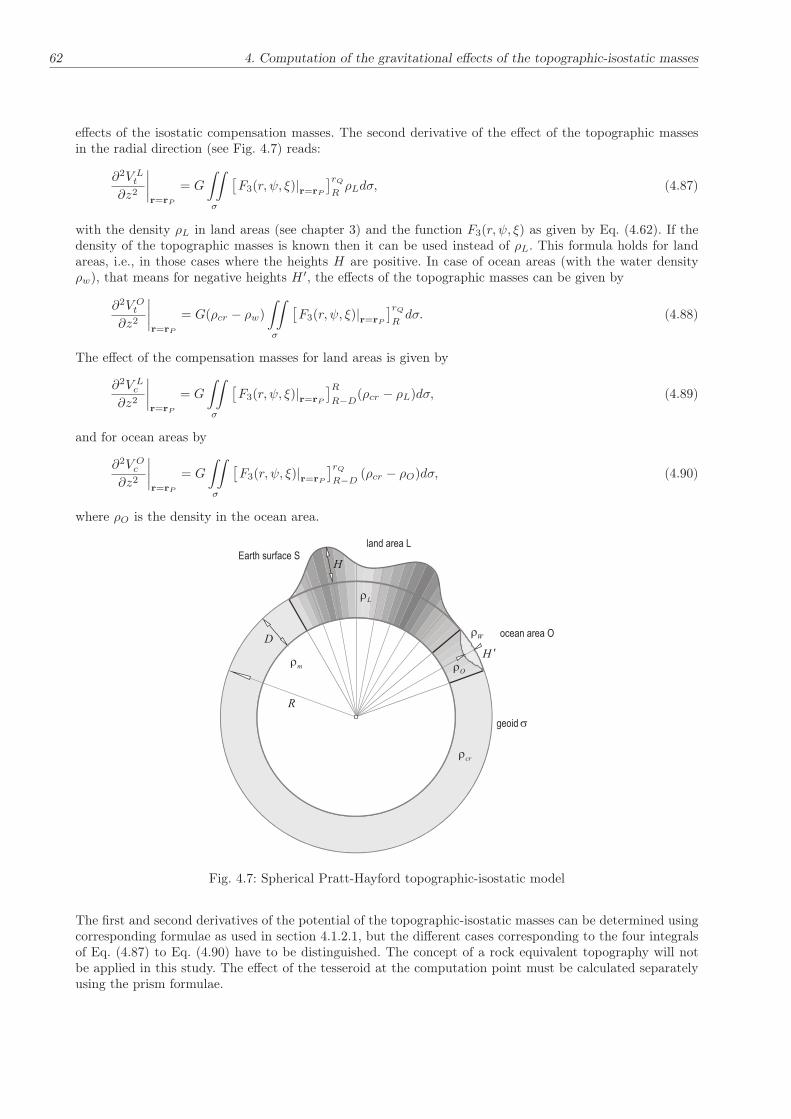
62 4. Computation of the gravitational effects of the topographic-isostatic masses
effects of the isostatic compensation masses. The second derivative of the effect of the topographic massesin the radial direction (see Fig. 4.7) reads:
∂2V Lt∂z2
∣∣∣∣r=rP
= G
∫∫
σ
[F3(r, ψ, ξ)|r=rP
]rQ
RρLdσ, (4.87)
with the density ρL in land areas (see chapter 3) and the function F3(r, ψ, ξ) as given by Eq. (4.62). If thedensity of the topographic masses is known then it can be used instead of ρL. This formula holds for landareas, i.e., in those cases where the heights H are positive. In case of ocean areas (with the water densityρw), that means for negative heights H ′, the effects of the topographic masses can be given by
∂2V Ot∂z2
∣∣∣∣r=rP
= G(ρcr − ρw)
∫∫
σ
[F3(r, ψ, ξ)|r=rP
]rQ
Rdσ. (4.88)
The effect of the compensation masses for land areas is given by
∂2V Lc∂z2
∣∣∣∣r=rP
= G
∫∫
σ
[F3(r, ψ, ξ)|r=rP
]R
R−D(ρcr − ρL)dσ, (4.89)
and for ocean areas by
∂2V Oc∂z2
∣∣∣∣r=rP
= G
∫∫
σ
[F3(r, ψ, ξ)|r=rP
]rQ
R−D(ρcr − ρO)dσ, (4.90)
where ρO is the density in the ocean area.
H ¢
Wr
Lr
mr
R
D
H
geoid s
Or
crr
land area LEarth surface S
ocean area O
Fig. 4.7: Spherical Pratt-Hayford topographic-isostatic model
The first and second derivatives of the potential of the topographic-isostatic masses can be determined usingcorresponding formulae as used in section 4.1.2.1, but the different cases corresponding to the four integralsof Eq. (4.87) to Eq. (4.90) have to be distinguished. The concept of a rock equivalent topography will notbe applied in this study. The effect of the tesseroid at the computation point must be calculated separatelyusing the prism formulae.

4.1. Direct integration method 63
Combined Airy-Pratt model The effects of the topographic-isostatic masses in land areas are calculatedaccording to the Airy-Heiskanen model and the effects of the topographic-compensation masses in ocean areasaccording to the Pratt-Hayford model.
4.1.2.3 Effect of the condensation masses
In Helmert’s methods of condensation, the compensation masses are condensed on a mass layer at a depthD1 below the geoidal sphere (Helmert’s first method of condensation) or on the geoid (Helmert’s secondmethod of condensation) which provides a simpler integral kernel. The potential of the condensed masses atthe computation point P can be given by (Heiskanen and Moritz 1967):
Vc|r=rP= G
∫∫
σ
kQlc
∣∣∣∣r=rP
R2cdσ, (4.91)
with the spatial distance
lc(r, ψ,Rc) =√
r2 +R2c − 2rRc cosψ, (4.92)
the density of the surface layer kQ, and the radius of the condensation sphere Rc. In case of Helmert’s firstcondensation method or generalized Helmert model of condensation it holds Rc = R − D1, and in caseof Helmert’s second condensation method Rc = R (see Fig. 4.8). In order to relate the potential of the
clHelmert 1:
Helmert 2 :cl
cR R=
Helmert 2:
1cR R D= -
Helmert 1:
Earth surface S
integration point
computation point
layer density Qk
P
Qr Q
geoid s
Pr
PH ¢
R
P¢
P¢r
ds
y
P Pr R H¢ ¢= + R
1D
ds
Pk ¢
Fig. 4.8: Geometry of Helmert’s condensation models
condensed masses to the potential of the topography the layer density kQ has to be given as a function ofthe topographical heights. It holds in spherical approximation (see chapter 3):
kQ = ρcrr3Q −R3
3R2c
. (4.93)

64 4. Computation of the gravitational effects of the topographic-isostatic masses
By adding and subtracting the density corresponding to the point P ′, the integral in Eq. (4.91) can bewritten in the following form (Heck 2003):
Vc|r=rP=
4πGkP ′R2c
r
∣∣∣∣r=rP
+GR2c
∫∫
σ
kQ − kP ′
lc(r, ψ,Rc)
∣∣∣∣r=rP
dσ
=4πGρ(r3P ′ −R3)
3r
∣∣∣∣r=rP
+GR2c
∫∫
σ
kQ − kP ′
lc(r, ψ,Rc)
∣∣∣∣r=rP
dσ.
(4.94)
The first term of Eq. (4.94) represents the effect of the condensation layer with the layer density kP ′ . Thefirst derivative of the potential of the condensation masses at P , (Vc)z, with the layer density kP ′ can bedetermined by differentiation of Eq. (4.94) with respect to r as follows:
∂Vc∂z
∣∣∣∣r=rP
=∂Vc∂r
∣∣∣∣∣r=rP
= − 4πGkP ′R2c
r2
∣∣∣∣r=rP
−G
∫∫
σ
(kQ − kp′)
l3c(r, ψ,Rc)(r −Rc cosψ)
∣∣∣∣∣∣r=rP
R2cdσ. (4.95)
Inserting the relation
r −Rc cosψ
l3c(r, ψ,Rc)
∣∣∣∣r=rP
=1
2r
(1
lc(r, ψ,Rc)+
r2 −R2c
l3c(r, ψ,Rc)
)∣∣∣∣r=rP
, (4.96)
the formula can be rewritten in the form:
∂Vc∂z
∣∣∣∣r=rP
= − 4πGρcr(r3P ′ −R3)
3r2
∣∣∣∣r=rP
−
− GρcrrP
∫∫
σ
(
r3Q − r3p′
6
) (r2 −R2
c
l3c(r, ψ,Rc)+
1
lc(r, ψ,Rc)
)∣∣∣∣r=rP
dσ.
(4.97)
Following a procedure as applied for the determination of Eq. (4.50) and Eq. (4.57), the first derivatives ofthe condensation masses with respect to x and y, (Vc)x and (Vc)y, are given by:
∂Vc∂x
∣∣∣∣r=rP
= −GρcrrP
∫∫
σ
(
r3Q − r3p′
3
)
Rcr sinψ
l3c(r, ψ,Rc)
∂ψ
∂ϕ
∣∣∣∣r=rP
dσ, (4.98)
∂Vc∂y
∣∣∣∣r=rP
= − GρcrrP cosϕ
∫∫
σ
(
r3Q − r3p′
3
)
Rcr sinψ
l3c(r, ψ,Rc)
∂ψ
∂λ
∣∣∣∣r=rP
dσ. (4.99)
where ∂ψ/∂ϕ and ∂ψ/∂λ are given by Eq. (4.53) and Eq. (4.58), respectively.
The second derivatives of the potential of the condensation masses in radial direction, (Vc)zz, can be deter-mined by differentiating Eq. (4.97) with respect to r and using Eq. (4.96), so that it follows:
∂2Vc∂z2
∣∣∣∣r=rP
=8πGρcr(r
3P ′ −R3)
3r3
∣∣∣∣r=rP
+
+Gρcrr2P
∫∫
σ
(
r3Q − r3p′
4
) (
(r2 −R2c)
2
l5c(r, ψ,Rc)− 4r2
3l3c(r, ψ,Rc)
+ 2
(r2 −R2
c
)
l3c(r, ψ,Rc)+
1
lc(r, ψ,Rc)
)∣∣∣∣∣r=rP
dσ.
(4.100)

4.1. Direct integration method 65
The second derivatives of the potential of the condensation masses in x direction, (Vc)xx, can be determinedaccording to Eq. (4.63) with the first term of this equation as given by Eq. (4.97) and the second term asgiven by:
1
r2∂2Vt∂ϕ2
∣∣∣∣r=rP
=Gρcrr2P
∫∫
σ
(
r3Q − r3p′
3
)[
−Rc sinψrl−3c (r, ψ,Rc)
∂2ψ
∂ϕ2+
+(−Rcr cosψl−3
c (r, ψ,Rc) + 3R2cr
2 sin2 ψl−5c (r, ψ,Rc)
)(∂ψ
∂ϕ
)2]∣∣∣∣∣r=rP
dσ,
(4.101)
based on Eq. (4.64) and Eq. (4.98), where ∂Vt/∂ψ and ∂2Vt/∂ψ2 are given by Eq. (4.55) and Eq. (4.66),
respectively. The formula used for calculating the second derivatives with respect to y, (Vc)yy, is given byEq. (4.69) with the first term given in Eq. (4.97) and the third term in Eq. (4.98). The second term of thisequation can be derived based on Eq. (4.70) and Eq. (4.99) as follows:
1
r2 cos2 ϕ
∂2Vc∂λ2
∣∣∣∣r=rP
=1
r2 cos2 ϕ
∂2Vc∂ψ2
(∂ψ
∂λ
)2∣∣∣∣∣r=rP
+1
r2 cos2 ϕ
∂Vc∂ψ
∂2ψ
∂λ2
∣∣∣∣r=rP
=Gρcr
r2P cos2 ϕ
∫∫
σ
r3Q − r3p′
3
[−Rcr cosψl−3
c (r, ψ,Rc) + 3R2cr
2 sin2 ψl−5c (r, ψ,Rc)
](∂ψ
∂λ
)2∣∣∣∣∣r=rP
dσ−
− Gρcrr2P cos2 ϕ
∫∫
σ
(r3Q − r3P ′
)
3Rcr sinψl−3
c (r, ψ,Rc)∂2ψ
∂λ2
∣∣∣∣r=rP
dσ,
(4.102)
where ∂ψ/∂λ and ∂2ψ/∂λ2 due to Eq. (4.58) and Eq. (4.71), respectively. The mixed second derivatives ofthe potential with respect to xz and xy, (Vc)xz and (Vc)xy, read as follows:
∂2Vc∂x∂z
∣∣∣∣r=rP
= −1
r
∂Vc∂ϕ
∣∣∣∣r=rP
+1
r
∂2Vc∂ϕ∂r
∣∣∣∣r=rP
, (4.103)
∂2Vc∂x∂y
∣∣∣∣r=rP
=tanϕ
r
∂Vc∂y
∣∣∣∣r=rP
+1
r2 cosϕ
∂2Vc∂ϕ∂λ
∣∣∣∣r=rP
. (4.104)
The first terms of Eq. (4.103) and Eq. (4.104) are calculated using Eq. (4.98) and Eq. (4.99), respectively.The second term of Eq. (4.103) can be determined using the following equation:
1
r
∂2Vc∂ϕ∂r
∣∣∣∣r=rP
=Gρ
rP
∫∫
σ
(
r3Q − r3p′
3
)
[−Rc sinψ l−3(r, ψ,Rc)+
+3Rcr sin nψ(r −Rc cosψ)l−5(r, ψ,Rc)] ∂ψ
∂ϕ
∣∣∣∣r=rP
dσ.
(4.105)
The second term of Eq. (4.104) is given by
1
r2 cosϕ
∂2Vc∂ϕ∂λ
∣∣∣∣r=rP
=1
r2P cosϕ
∫∫
σ
(r3Q − r3P ′)
3([−Rcr cosψ l−3(r, ψ,Rc) + 3R2
cr2 sin2 ψl−5(r, ψ,Rc)
].
.∂ψ
∂λ
∂ψ
∂ϕ− Rcr sinψ
l3c(r, ψ,Rc)
∂2ψ
∂ϕ∂λ
)∣∣∣∣r=rp
dσ,
(4.106)
where ∂ψ/∂ϕ, ∂ψ/∂λ and ∂2ψ/∂ϕ∂λ are given by Eq. (4.53), Eq. (4.58) and Eq. (4.81), respectively. Finally,the effect of the condensation masses in yz - direction, (Vc)yz, is calculated as follows:
∂2Vc∂y∂z
∣∣∣∣r=rP
= −1
r
∂Vc∂y
∣∣∣∣r=rP
+1
r cosϕ
∂2Vc∂λ∂r
∣∣∣∣r=rP
, (4.107)

66 4. Computation of the gravitational effects of the topographic-isostatic masses
with the first term given by Eq. (4.99). The second term can be determined based on Eq. (4.78) as follows:
1
r cosϕ
∂2Vc∂λ∂r
∣∣∣∣r=rP
= − GρcrrP
∫∫
σ
r3Q − r3P ′
3[−Rc sinψ l−3(r, ψ,Rc)+
+3Rcr sinψ(r −Rc cosψ)l−5(r, ψ,Rc)]sinαQ
∣∣r=rP
dσ.
(4.108)
4.2 Spherical harmonic expansion
In this section, an algorithm for the computation of the spherical harmonic expansion of the topographic-isostatic masses from a digital terrain model (DTM) is presented. The method is based on a series expansionof the inverse distance function – the kernel function of the Newtonian potential. The isostatic compensationof the topography for different topographic-isostatic models is taken into account. This method is appropriateespecially for satellite applications. For airborne gravimetry and for gravimetry at the Earth surface a methodis presented for the calculation of far-zone effects of the topographic-isostatic masses.
4.2.1 Effects of topographic-isostatic masses in satellite applications
4.2.1.1 The effect of topographic masses
For determining the effect of topographic masses, again we start with the formula for the gravitationalpotential of the Earth at any point P on or outside the Earth’s surface as it is given by Newton’s law ofgravitation,
V t∣∣r=rP
= G
∫∫∫
v
ρ(Q)
l
∣∣∣∣r=rP
dv. (4.109)
The distance between the computation point P and the source point Q, l|r=rP, is given by Eq. (4.38). The
gravitational potential is harmonic outside the masses and its spherical harmonic expansion is convergentoutside a sphere enclosing the total mass of the Earth (see chapter 2). The series expansion for the inversedistance l|r=rP
in spherical coordinates can be written as follows (Heiskanen and Moritz 1967, Eq. 1.81):
[l|r=rP
]−1=
∞∑
n=0
ξn
rn+1P
Pn(cosψPQ) for rP > ξ
∞∑
n=0
rnPξn+1
Pn(cosψPQ) for rP < ξ
, (4.110)
where Pn(cosψPQ) are the Legendre polynomials of degree n and ψPQ is the spherical distance between thegeocentric direction of points P and Q which can be computed by the spherical angle cosine theorem,
cosψPQ = cosϕ cosϕQ + sinϕ sinϕQ cos(λ− λQ). (4.111)
Firstly, we refer to a computation point outside the sphere enclosing the total masses of the Earth (forcalculating the effect of topographic and isostatic masses at aeroplane or at satellite altitude). Therefore,only the first term of Eq. (4.110) is taken into consideration. The second term has been described in Engelsand Grafarend (1993). Applying the addition theorem of the spherical harmonic functions to separate thecoordinate dependencies related to point P from those related to point Q gives
Pn(cosψPQ) =1
2n+ 1
n∑
m=0
Pnm(cos θ)Pnm(cos θQ)·
· [cosmλ cosmλQ + sinmλ sinmλQ] ,
(4.112)

4.2. Spherical harmonic expansion 67
where Pnm are the fully normalized associated Legendre functions of degree n and order m. Then the inversedistance can be written as follows (Rummel et al. 1988):
[l|r=rP
]−1=
1
rP
∑
n,m,α
(ξ/rP )n 1
2n+ 1Y αnm(p)Y αnm(Q), (4.113)
with the surface spherical harmonics
Y α=0nm = Pmn (cos θ) cosmλ,
Y α=1nm = Pmn (cos θ) sinmλ.
(4.114)
By substituting Eq. (4.113) with Eq. (4.114) into Eq. (4.109), the gravitational potential can be written asfollows (Tsoulis 1999a):
V t∣∣r=rP
=G
∫∫∫
v
ρ(Q)1
rp
∞∑
n=0
(ξ
rp
)n1
2n+ 1
n∑
m=0
1∑
α=0
Y αnm(P )Y αnm(Q)dv,
=GM
R
∞∑
n=0
Rn+1
rn+1P
n∑
m=0
1∑
α=0
Y αnm(P )Cα,Tnm ,
(4.115)
with the mass of the Earth M , the mean Earth radius R, the fully normalized spherical harmonic coefficientsCαnm and the density function
ρ(Q) =
{
ρ(Q) in land areas
ρw − ρcr in ocean areas
}
. (4.116)
Then the potential coefficients of the topographic masses can be given by (Rummel et al. 1988):
Cα,Tnm =1
M(2n+ 1)
∫∫∫
v
(ξ
R
)n
ρ(ξ)Y αnm(ξ)dv, (4.117)
with the total mass of the Earth in spherical approximation,
M = 4πρR3/3, (4.118)
where ρ is the mean density of the Earth . After introducing the volume of the integration element in sphericalcoordinates dv = ξ2dξdσ, the spherical harmonic coefficients of the potential of the topographic masses canbe written in the following form:
Cα,Tnm =3
ρR(2n+ 1)
1
4π
∫∫
σ
AT (Q)Y αnmdσ, (4.119)
where the surface topography part AT (Q) in case of topographic masses above the geoid is given by
AT (Q) =
rs∫
ξ=rg
ρ(Q)
(ξ
R
)n+2
dξ. (4.120)
The quantities rg and rs are the radius of the geoid and the surface of the Earth, respectively. After integrationEq. (4.120) results in:
AT (Q) =
[
R
n+ 3ρ(Q)
(ξ
R
)n+3]rs
rg
= ρ(Q)R
n+ 3
[(rsR
)n+3
−(rgR
)n+3]
= ρ(Q)R
n+ 3
[(
1 +rs −R
R
)n+3
−(
1 +rg −R
R
)n+3]
.
(4.121)

68 4. Computation of the gravitational effects of the topographic-isostatic masses
After some algebraic operations Eq. (4.121) can be written in the following form:
AT (Q) = ρ(Q)R
([(rs −R
R
)
−(rg −R
R
)]
+n+ 2
2
[(rs −R
R
)2
−(rg −R
R
)2]
+
+(n+ 2)(n+ 1)
6
[(rs −R
R
)3
−(rg −R
R
)3]
+1
n+ 3
n+3∑
k=4
(n+ 3
k
)[(rs −R
R
)k
−(rg −R
R
)k])
.
(4.122)
Inserting Eq.(4.122) into Eq.(4.119) gives the potential coefficients of the topographic masses as follows:
Cα,Tnm =3
(2n+ 1)ρ
{
R1αnm +n+ 2
2R2αnm+
(n+ 1)(n+ 2)
6R3αnm +
1
n+ 3
n+3∑
k=4
(n+ 3
k
)
Rkαnm
}
, (4.123)
with the coefficients
R1αnm =1
4π
∫∫
σ
[(rs −R
R
)
−(rg −R
R
)]
ρ(Q)Y αnmdσ =1
4π
∫∫
σ
[(HQ −NQ
R
)]
ρ(Q)Y αnmdσ, (4.124)
Rkαnm =1
4π
∫∫
σ
[(rs −R
R
)k
−(rg −R
R
)k]
ρ(Q)Y αnmdσ1
4π
∫∫
σ
[(
HkQ −Nk
Q
Rk
)]
ρ(Q)Y αnmdσ, (4.125)
where N is the geoid heights.
If the geoid is approximated by a sphere with a radius equal to the mean Earth radius, the surface topographypart (Eq. 4.120) will be transformed to:
AT (Q) =
ξ=R+HQ∫
ξ=R
ρ(Q)
(ξ
R
)n+2
dξ, (4.126)
with the topographic or bathymetric height H or H ′, respectively. If the topography columns consist ofseveral layers with constant densities in each layer (see chapter 3), then the surface topography part iswritten as:
AT (Q) =l∑
i=0
ξ=R+Hi∫
ξ=R
(ρi(Q) − ρi+1(Q))
(ξ
R
)n+2
dξ =l∑
i=0
ξ=R+Hi∫
ξ=R
δρi(Qi)
(ξ
R
)n+2
dξ, (4.127)
where ρi(Q) is the density of every topographic layer; ρ0, ρl+1 are defined in chapter 3. After performing theintegration with respect to ξ, Eq. (4.127) results in
AT (Q) =R
l∑
i=0
(ρi(Q) − ρi+1(Q))
[
Hi
R+
(n+ 2)
2
(Hi
R
)2
+(n+ 2)(n+ 1)
6
(Hi
R
)3
+
+1
n+ 3
n+3∑
k=4
(n+ 3
k
)(Hi
R
)k]
.
(4.128)
Insertion of Eq. (4.128) into Eq. (4.119) gives the potential coefficients of the topographic masses in sphericalapproximation,
Cα,Tnm =3
(2n+ 1)ρ
{
ha1αnm +n+ 2
2ha2αnm+
(n+ 1)(n+ 2)
6ha3αnm +
1
n+ 3
n+3∑
k=4
(n+ 3
k
)
hakαnm
}
, (4.129)
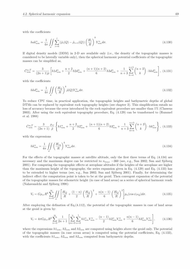
4.2. Spherical harmonic expansion 69
with the coefficients
hakαnm =1
4π
∫∫
σ
l∑
i=0
(ρi(Q) − ρi+1(Q))
(Hi
R
)k
Y αnmdσ. (4.130)
If digital density models (DDM) in 2-D are available only (i.e., the density of the topographic masses isconsidered to be laterally variable only), then the spherical harmonic potential coefficients of the topographicmasses can be simplified as,
Cα,Tnm =3
(2n+ 1)ρ
[
h1dαnm +n+ 2
2h2dαnm +
(n+ 1)(n+ 2)
6h3dαnm +
1
n+ 3
n+3∑
k=4
(n+ 3
k
)
· hkdαnm
]
, (4.131)
with the coefficients
hkdαnm =1
4π
∫∫
σ
(HQ
R
)k
ρ(Q)Y αnmdσ. (4.132)
To reduce CPU time, in practical application, the topographic heights and bathymetric depths of globalDTMs can be replaced by equivalent rock topography heights (see chapter 3). This simplification entails noloss of accuracy because the error introduced by the rock equivalent procedure are smaller than 1% (Classens2003). After using the rock equivalent topography procedure, Eq. (4.129) can be transformed to (Rummelet al. 1988)
Cα,Tnm =3
(2n+ 1)
ρcrρ
{
h1αnm +n+ 2
2h2αnm +
(n+ 1)(n+ 2)
6h3αnm +
1
n+ 3
n+3∑
k=4
(n+ 3
k
)
· hkαnm
}
, (4.133)
with the expressions
hkαnm =1
4π
∫∫
σ
(Heq
R
)k
Y αnmdσ. (4.134)
For the effects of the topographic masses at satellite altitude, only the first three terms of Eq. (4.134) arenecessary and the maximum degree can be restricted to nmax =360 (see, e.g., Sun 2002; Sun and Sjöberg2001). For computing the topographic effects at aeroplane altitudes if the heights of the aeroplane are higherthan the maximum height of the topography, the series expansion given in Eq. (4.129) and Eq. (4.133) hasto be extended to higher terms (see, e.g., Sun 2002; Sun and Sjöberg 2001). Finally, for determining theindirect effect the computation point is taken to be at the geoid. Then convegent expansion of the potentialof the topographic masses for othometric height (in case of land areas) as a series of spherical harmonic reads(Nahavandchi and Sjöberg 1998):
Vt = GρcrR2
∞∑
n=0
∫∫
σ
[
HQ
R+
(1 − n)
2
(HQ
R
)2
+n(n− 1)
6
(HQ
R
)3]
pn(cosψPQ)dσ. (4.135)
After employing the defination of Eq.(4.112), the potential of the topographic masses in case of land areasat the geoid is given by:
Vt = 4πGρcrR2
∞∑
n=0
1
2n+ 1
[n∑
m=0
1∑
α=0
h1αnmYαnm − (n− 1)
2h2αnmY
αnm +
n(n− 1)
6h3αnmY
αnm
]
, (4.136)
where the expressions h1nm, h2nm and h2nm are computed using heights above the geoid only. The potentialof the topographic masses (in case ocean areas) is computed using the potential coefficients, Eq. (4.133),with the coefficients h1nm, h2nm and h2nm computed from bathymetric depths.

70 4. Computation of the gravitational effects of the topographic-isostatic masses
4.2.1.2 Effect of the isostatic masses
The topographic-isostatic models due to Airy-Heiskanen, Vening-Meinesz, Pratt-Hayford and the combinedAiry-Pratt model as well as Helmert’s first and second condensation methods will be formulated in terms ofspherical harmonic expansions in the following.
Airy-Heiskanen model The spherical harmonic coefficients of the isostatic masses can be derived similarto those of the topographic masses according to Eq. (4.119) (e.g. Rummel et al. 1988):
Cα,Cnm =3
ρR(2n+ 1)
1
4π
∫∫
σ
AC(Q)Y αnmdσ, (4.137)
where the isostatic compensation masses are covered by
AC(Q) =
R−T∫
R−T−tQ
∆ρ
(ξ
R
)n+2
dξ, (4.138)
with the thickness of the crust T and the difference in density between the crust and the mantle ∆ρ = ρm−ρcr.After performing the integration, the isostatic compensation part is given by:
AC(Q) = ∆ρR
n+ 3
[(R− T )
R
)n+3
−(R− T − tQ
R
)n+3]
. (4.139)
Eq. (4.139) can be written in the following form:
AC(Q) =∆ρR
n+ 3
[(R− T )
R
)n+3
−(R− T
R
)n+3(
1 − (n+ 3)tQ
(R− T )+
(n+ 2)(n+ 3)
2.
.
(tQ
R− T
)2
− (n+ 3)(n+ 2)(n+ 1)
6
(tQ
R− T
)3
+1
(n+ 3)
n+3∑
k=4
(n+ 3
k
)( −tQR− T
)k)]
,
(4.140)
and after some algebraic rearrangements,
AC(Q) =∆ρR
(R− T )
R
)n+2 [tQR
− R(n+ 2)
2(R− T )
(tQR
)2
+R2(n+ 2)(n+ 1)
6(R− T )2
(tQR
)3
−
− 1
(n+ 3)
n+3∑
k=4
(n+ 3
k
)(−tQR
)k (R
R− T
)k−1]
.
(4.141)
The potential coefficients of the isostatic masses read analogously to Eq. (4.133)
Cα,Cnm =3∆ρ
(2n+ 1)ρ
(R− T )
R
)n+2 [
t1αnm − R(n+ 2)
2(R− T )t2αnm+
R2(n+ 2)(n+ 1)
6(R− T )2t3nm−
− 1
(n+ 3)
n+3∑
k=4
(n+ 3
k
)(R
R− T
)k−1
(−1)k · tkαnm
]
,
(4.142)
with the terms
tkαnm :=1
4π
∫∫
σ
(tQR
)k
Y αnmdσ. (4.143)
The roots and anti-roots are determined based on the formulae as given in chapter 3.
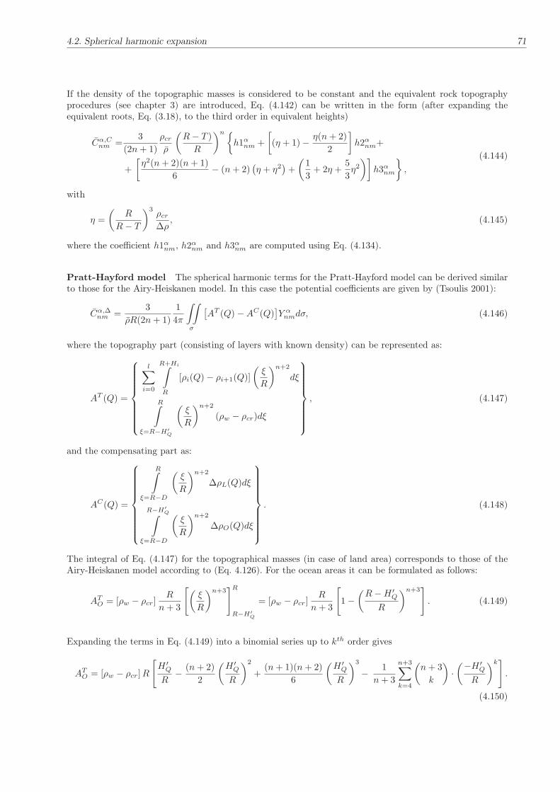
4.2. Spherical harmonic expansion 71
If the density of the topographic masses is considered to be constant and the equivalent rock topographyprocedures (see chapter 3) are introduced, Eq. (4.142) can be written in the form (after expanding theequivalent roots, Eq. (3.18), to the third order in equivalent heights)
Cα,Cnm =3
(2n+ 1)
ρcrρ
(R− T )
R
)n{
h1αnm +
[
(η + 1) − η(n+ 2)
2
]
h2αnm+
+
[η2(n+ 2)(n+ 1)
6− (n+ 2)
(η + η2
)+
(1
3+ 2η +
5
3η2
)]
h3αnm
}
,
(4.144)
with
η =
(R
R− T
)3ρcr∆ρ
, (4.145)
where the coefficient h1αnm, h2αnm and h3αnm are computed using Eq. (4.134).
Pratt-Hayford model The spherical harmonic terms for the Pratt-Hayford model can be derived similarto those for the Airy-Heiskanen model. In this case the potential coefficients are given by (Tsoulis 2001):
Cα,∆nm =3
ρR(2n+ 1)
1
4π
∫∫
σ
[AT (Q) −AC(Q)
]Y αnmdσ, (4.146)
where the topography part (consisting of layers with known density) can be represented as:
AT (Q) =
l∑
i=0
R+Hi∫
R
[ρi(Q) − ρi+1(Q)]
(ξ
R
)n+2
dξ
R∫
ξ=R−H′
Q
(ξ
R
)n+2
(ρw − ρcr)dξ
, (4.147)
and the compensating part as:
AC(Q) =
R∫
ξ=R−D
(ξ
R
)n+2
∆ρL(Q)dξ
R−H′
Q∫
ξ=R−D
(ξ
R
)n+2
∆ρO(Q)dξ
. (4.148)
The integral of Eq. (4.147) for the topographical masses (in case of land area) corresponds to those of theAiry-Heiskanen model according to (Eq. 4.126). For the ocean areas it can be formulated as follows:
ATO = [ρw − ρcr]R
n+ 3
[(ξ
R
)n+3]R
R−H′
Q
= [ρw − ρcr]R
n+ 3
[
1 −(R−H ′
Q
R
)n+3]
. (4.149)
Expanding the terms in Eq. (4.149) into a binomial series up to kth order gives
ATO = [ρw − ρcr]R
[
H ′
Q
R− (n+ 2)
2
(H ′
Q
R
)2
+(n+ 1)(n+ 2)
6
(H ′
Q
R
)3
− 1
n+ 3
n+3∑
k=4
(n+ 3
k
)
·(−H ′
Q
R
)k]
.
(4.150)

72 4. Computation of the gravitational effects of the topographic-isostatic masses
Then, the contribution of the oceanic part to the potential coefficients can be given analogously to Eq. (4.133)by:
Cα,T,Onm =3
2n+ 1
(ρw − ρcr)
ρ
{
h′1αnm − n+ 2
2h′2αnm +
(n+ 1)(n+ 2)
6h′3αnm−
− 1
n+ 3
n+3∑
k=4
(n+ 3
k
)
· (−1)kh′kαnm
}
,
(4.151)
with the coefficients
h′kαnm =1
4π
∫∫
σ
(H ′
Q
R
)k
Y αnmdσ. (4.152)
For calculating the effect of the compensating masses in case of the land part (upper term of Eq. 4.148), thedensity deficiency is calculated as follows:
∆ρL(Q) = ρcr − ρL(Q). (4.153)
Inserting this relation into the first term of Eq. (4.148) and integrating over rQ yields:
ACL = ∆ρL(Q)R
n+ 3
[
1 −(R−D
R
)n+3]
. (4.154)
Similarly, the density surplus for the suboceanic columns is given by:
∆ρO(Q) = ρcr − ρO(Q), (4.155)
where ρO and ρL are calculated using the formulae in chapter 3. Inserting Eq. (4.155) in the lower term ofEq. (4.148) and integrating over ξ gives the contribution for the oceanic areas:
ACO =∆ρO(Q)R
[
−(H ′
Q
R
)
+n+ 2
2
(H ′
Q
R
)2
− (n+ 2)(n+ 1)
6
(H ′
Q
R
)3
+
+1
n+ 3
n+3∑
k=4
(n+ 3
k
)
·(−H ′
Q
R
)k]
+ ∆ρoceanR
n+ 3
[
1 −(R−D
R
)n+3]
.
(4.156)
Finally, the potential coefficients of the compensating masses for land areas read
Cα,C,Lnm =3
ρ(2n+ 1)(n+ 3)
[
1 −(R−D
R
)n+3]
hαdh, (4.157)
and for ocean areas
Cα,C,Onm =3
ρ(2n+ 1)
{
−h′′1αnm +n+ 2
2h′′2αnm − (n+ 1)(n+ 2)
6h′′3αnm+
+1
n+ 3
n+3∑
k=4
(n+ 3
k
)
· (−1)kh′′kαnm
}
+3
(2n+ 1)(n+ 3)ρ
[
1 −(R−D
R
)n+3]
h′′αdh,
(4.158)
with the terms
hαdh =1
4π
∫∫
σ
∆ρL(Q)Y αnmdσ, (4.159)
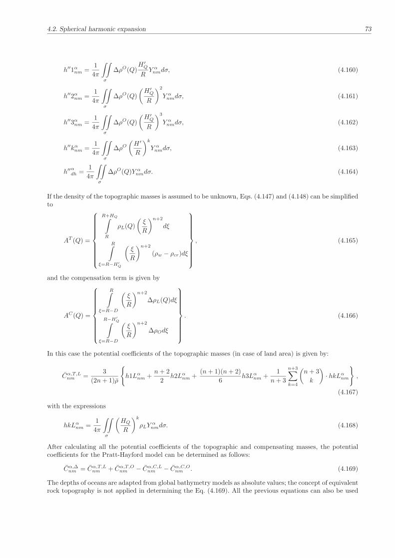
4.2. Spherical harmonic expansion 73
h′′1αnm =1
4π
∫∫
σ
∆ρO(Q)H ′
Q
RY αnmdσ, (4.160)
h′′2αnm =1
4π
∫∫
σ
∆ρO(Q)
(H ′
Q
R
)2
Y αnmdσ, (4.161)
h′′3αnm =1
4π
∫∫
σ
∆ρO(Q)
(H ′
Q
R
)3
Y αnmdσ, (4.162)
h′′kαnm =1
4π
∫∫
σ
∆ρO(H ′
R
)k
Y αnmdσ, (4.163)
h′′αdh =
1
4π
∫∫
σ
∆ρO(Q)Y αnmdσ. (4.164)
If the density of the topographic masses is assumed to be unknown, Eqs. (4.147) and (4.148) can be simplifiedto
AT (Q) =
R+HQ∫
R
ρL(Q)
(ξ
R
)n+2
dξ
R∫
ξ=R−H′
Q
(ξ
R
)n+2
(ρw − ρcr)dξ
, (4.165)
and the compensation term is given by
AC(Q) =
R∫
ξ=R−D
(ξ
R
)n+2
∆ρL(Q)dξ
R−H′
Q∫
ξ=R−D
(ξ
R
)n+2
∆ρOdξ
. (4.166)
In this case the potential coefficients of the topographic masses (in case of land area) is given by:
Cα,T,Lnm =3
(2n+ 1)ρ
{
h1Lαnm +n+ 2
2h2Lαnm +
(n+ 1)(n+ 2)
6h3Lαnm +
1
n+ 3
n+3∑
k=4
(n+ 3
k
)
· hkLαnm
}
,
(4.167)
with the expressions
hkLαnm =1
4π
∫∫
σ
(HQ
R
)k
ρLYαnmdσ. (4.168)
After calculating all the potential coefficients of the topographic and compensating masses, the potentialcoefficients for the Pratt-Hayford model can be determined as follows:
Cα,∆nm = Cα,T,Lnm + Cα,T,Onm − Cα,C,Lnm − Cα,C,Onm . (4.169)
The depths of oceans are adapted from global bathymetry models as absolute values; the concept of equivalentrock topography is not applied in determining the Eq. (4.169). All the previous equations can also be used

74 4. Computation of the gravitational effects of the topographic-isostatic masses
for calculating the Pratt-Hayford model in planar approximation. Differences occur only in determining thevariable density (chapter 3). An alternative method can be developed in case of the unknown density of thetopography for computing the Pratt-Hayford compensation model: In this method the potential coefficientsof the topographic masses are considered to be equal the potential coefficients for the Airy-Heiskanen modeland the potential coefficients of the compensating masses are calculated in one step according to the followingequation:
Cα,∆nm =3
ρR(2n+ 1)
1
4π
∫∫
σ
[AT (Q) −AC(Q)
]Y αnmdσ, (4.170)
with the topography and compensation constituents
AT (Q) =
R+HQ∫
R
ρcr
(ξ
R
)n+2
dξ
R∫
ξ=R−H′
Q
(ξ
R
)n+2
(ρw − ρcr)dξ
, (4.171)
AC(Q) =
R+HQ∫
ξ=R−D
(ξ
R
)n+2
∆ρ(Q)dξ, (4.172)
where ∆ρ(Q) is the difference between the density of the integration element and the constant crust density incase of the land and ocean areas and H is the orthometric height in case of the topographic and bathymetricdepths in ocean areas. Eq. (4.171) is the same as the equation derived for the Airy-Heiskanen model forcalculating the effects of the topographic masses. After integration and insertion of the integral limits, Eq.(4.172) can be written as:
AC(Q) =∆ρ(Q)R
[(HQ
R
)
+n+ 2
2
(HQ
R
)2
+(n+ 2)(n+ 1)
6
(HQ
R
)3
+
+1
n+ 3
n+3∑
k=4
(n+ 3
k
)
·(HQ
R
)k]
+ ∆ρ(Q)R
n+ 3
[
1 −(R−D
R
)n+3]
.
(4.173)
Finally, the potential coefficients of the compensating masses for land and ocean areas are given by:
Cα,Cnm =3
ρ(2n+ 1)
{
hbαnm +n+ 2
2h2bαnm +
(n+ 1)(n+ 2)
6h3bαnm+
+1
n+ 3
n+3∑
k=4
(n+ 3
k
)
· hkbαnm
}
+3
(2n+ 1)(n+ 3)ρ
[
1 −(R−D
R
)n+3]
hαdh,
(4.174)
with the coefficients
hkbαnm =1
4π
∫∫
σ
∆ρ(Q)
(HQ
R
)k
Y αnmdσ. (4.175)
Combined Airy-Pratt model In this model the potential coefficients of the topographic and isostaticcompensation masses for continental areas are computed according to the Airy-Heiskanen model and the

4.2. Spherical harmonic expansion 75
potential coefficients of the topographic-isostatic compensation masses for ocean areas according to thePratt-Hayford model. The spherical harmonic coefficients read as follows,
cα,∆nm = cα,T,Lnm − cα,C,Lnm︸ ︷︷ ︸
Airy−Heiskanen model
+ cα,T,Onm − cα,C,Onm︸ ︷︷ ︸
Pratt−Hayford model
.(4.176)
In this investigation, the concept of rock equivalent topographic heights will not be applied in the case ofthe Pratt-Hayford and the combined Airy-Pratt models.
Vening-Meinesz isostatic model In case of the Vening-Meinesz model, the isostatic compensation partof the topography is filtered for small scale signals, i.e. for high frequencies. This can be taken into accountby using degree-dependent low-pass spectral smoothing filter coefficients βn for the compensation part.Inserting these filter coefficients into Eq. (4.144) results in the following equation for the spherical harmoniccompensation coefficients
cβ,α,Cnm = βn(nb, k)cα,Cnm . (4.177)
The spectral amplitude filter coefficients βn are defined as follows:
βn(nb, k) =
√
1
1 + (n/nb)2k, (4.178)
with the order k of the filter and the band degree nb at which the power (or the amplitude) is halved (cf.Haagmans 2000). The parameter k defines the steepness of the low-pass filter. For k = 0 the coefficients arenot filtered at all and for k = ∞ all the coefficients below nb are preserved and the coefficients above nb areset equal to zero. The choice of nb can be based upon the spatial scale for which the Airy-Heiskanen modelis no longer valid. Haagmans (2000) and Pail (2000) states that the compensation model is not likely to bevalid for topographic signals at spatial scales smaller than 200 km while Sjöberg (1998b) gives a value of500 km. The value of Haagmans corresponds more or less to the non-validity of the compensation model forfrequencies above degree 200. In this study, the parameters chosen by Haagmans (2000) are used as k = 3and nb = 150.
4.2.1.3 Helmert’s condensation methods
The potential due to the topographic masses in case of Helmert’s condensation methods is identical to that ofthe Airy-Heiskanen model Eq. (4.129). The potential of the condensed masses can be given by the followingequation (Heck 2003):
V c|r=rP= G
∫∫
σ
kQlc
∣∣∣∣r=rP
R2cdσ, (4.179)
where Rc is the radius of the condensed masses and kQ is the surface density at the integration point, Q.The surface density can be calculated using the formulae as given in chapter 3. The reciprocal of the distancecan be written as spherical harmonic expansion as follows:
l−1c = (r2 +R2
c − 2rRc cosψ)−12 =
1
r
∞∑
n=0
(Rcr
)n
Pn(cosψ). (4.180)
Inserting Eq. (4.180) into Eq. (4.179) with kQ as defined in chapter 3 yields:
V c|r=rP= GR2
c
∞∑
n=0
(R
rP
)n+1(RcR
)n ∫∫
σ
l∑
i=0
(ρi − ρi+1)
R2c
R3
[(Hi
R
)
+
(Hi
R
)2
+1
3
(Hi
R
)3]
Pn(cosψ)dσ.

76 4. Computation of the gravitational effects of the topographic-isostatic masses
(4.181)
Following the procedures that led to Eq. (4.129), the potential coefficients for the condensed masses aredetermined as follows:
Cα,Cnm =3
(2n+ 1)ρ
[(RcR
)n
haαnm +
(RcR
)n
ha2αnm +
(RcR
)n
ha3αnm
]
. (4.182)
The coefficients hakαnm are computed from Eq. (4.130).
Finally, the differences between the potential coefficients of the topographic and condensed masses read
cα,Inm =3
(2n+ 1)ρ
{[
1 −(RcR
)n]
ha1αnm +
[n+ 2
2−(RcR
)n]
ha2αnm+
+1
3
[(n+ 2)(n+ 1)
2−(RcR
)n]
ha3αnm +1
n+ 3
n+3∑
k=4
(n+ 3
k
)
· hakαnm
}
.
(4.183)
The quantity Rc is the radius of the (approximate) condensation sphere. In case of Helmert’s first or gene-ralized condensation method it holds Rc = R − D1, and in case of Helmert’s second condensation methodRc = R.
If the density of the topographic masses is considered to be constant or the rock equivalent topography isused, the potential coefficients of the topographic and condensed masses will be given by:
cα,Inm =3ρcr
(2n+ 1)ρ
{[
1 −(RcR
)n]
h1αnm +
(
[n+ 2
2−(RcR
)n]
h2αnm+
+1
3
[(n+ 2)(n+ 1)
2−(RcR
)n]
h3αnm +1
n+ 3
n+3∑
k=4
(n+ 3
k
)
· hkαnm
}
,
(4.184)
where the coefficients h1αnm, h2αnm, h3αnm and hkαnm are computed according to Eq. (4.134).
4.2.2 Spherical harmonic expansion for calculating the far-zone topographical effects
Let us start with the potential of the topographic masses as given by Newton’s integral
V t∣∣r=rP
= Gρcr
∫∫
σ
rQ∫
R
ξ2
l
∣∣∣∣r=rP
dξ
dσ. (4.185)
The integration domain is divided into two parts σ = σ0 ∪ σFz where σ0 is the near zone and σFz is thefar-zone. Then the integral in Eq. (4.185) can be written as the sum of the two parts as follows:
V t∣∣r=rP
= Gρcr
∫∫
σ0
R+HQ∫
R
ξ2
l
∣∣∣∣r=rP
dξ
dσ +Gρcr
∫∫
σF z
R+HQ∫
R
ξ2
l
∣∣∣∣r=rP
dξ
dσ
=: V t0∣∣r=rP
+ V tF z∣∣r=rP
.
(4.186)
Here we will study the term V tF z |r=rPor quantities related to this term. The quantity V tF z |r=rP
is expressedby a series expansion in terms of Laplace’s surface spherical harmonics. Then the truncation coefficients dueto Molodenskii will be derived to get an impression of the far-zone effects.

4.2. Spherical harmonic expansion 77
4.2.2.1 The direct topographical effects on gravity
Helmert’s second method of condensation The topographical masses are condensed on the geoid asa single layer. The direct topographical effect DTE on gravity was given by Martinec and Vaníček (1994b)in spherical approximation. DTE can be obtained from the difference between the first derivatives of thepotential of the topographic and the condensed masses as follows:
DTE(r, ϕ, λ)|r=rP=∂V
∂r
∣∣∣∣r=rP
= Gρcr
∫∫
σ
∂
∂r
R+HQ∫
ξ=R
l−1(r, ψ , ξ)|r=rPξ2dξdσ −Gρcr
∫∫
σ
R+HQ∫
ξ=R
ξ2dξ
∂
∂rl−1(r, ψ, R)|r=rP
dσ.
(4.187)
The reciprocal distance between the computation and the integration point is given by
l−1(r, ψ, ξ) = (r2 + ξ2 − 2rξ cosψ)−1/2, (4.188)
with the spherical distance ψ expressed as:
cosψ = cosϕ cosϕQ + sinϕ sinϕQ cos(λ− λQ). (4.189)
The contribution of the integral of Eq. (4.187) can be developed in the following form (Novák et al. 2001):
DTE|r=rP=Ab +Gρcr
∫∫
σ
R+HQ∫
ξ=R+HP ′
∂
∂rl−1(r, ψ, ξ) |r=rP
ξ2dξdσ−
−Acb −Gρcr
∫∫
σ
R+HQ∫
ξ=R+HP ′
∂
∂rl−1(r, ψ,R)
∣∣r=rP
ξ2dξdσ.
(4.190)
Ab and Acb are the gravitational effects of the topographical Bouguer shell and the corresponding Bouguerlayer. The terms Ab and Acb are equal if mass conservation is anticipated (Wichiencharoen 1982). In this caseboth terms cancel eact other. The difference between the other two terms is called the direct terrain effectDTEter in the following. The far-zone contribution can be determined in an economic approximative way.This section treats only the far-zone contribution of the topographic-condensation masses which is given byEq. (4.191) as derived in Appendix A.1.1:
DTEterF Z
∣∣r=rP
=2πGρcr
(Nmax∑
n=0
tn(η, ψ, ψ0)Hn(ϕ, λ)+1
rP
Nmax∑
n=0
un(η, ψ, ψ0)H2n(ϕ, λ)−
− 2HP
rP
Nmax∑
n=0
un(η, ψ, ψ0)Hn(ϕ, λ) −Nmax∑
n=0
wn(HP , ψ, ψ0)Hn(ϕ, λ)−
− 2(HP ′ −HP )
rP
Nmax∑
n=0
vn(η, ψ, ψ0)Hn(ϕ, λ) − 1
R
Nmax∑
n=0
wn(HP , ψ, ψ0)H2n(ϕ, λ)
)
+ [C1 − C2] ,
(4.191)
where tn(η, ψ, ψ0), un(η, ψ, ψ0), vn(η, ψ, ψ0) and wn(HP , ψ, ψ0) are Molodenskii’s truncation coefficients asdefined in Appendix A.1.1 by Eqs. (A.20), (A.25), (A.26) and (A.28), respectively. C1 and C2 are given byEqs. (A.27) and (A.37), respectively.
The Laplace surface spherical harmonics of the height function Hn(ϕ, λ) and the squared height functionH2n(ϕ, λ) are given by:
Hn(ϕ, λ) =
n∑
m=−n
Hn,mYn,m(ϕ, λ), H2n(ϕ, λ) =
n∑
m=−n
H2n,mYn,m(ϕ, λ), (4.192)

78 4. Computation of the gravitational effects of the topographic-isostatic masses
where the coefficientsHn,m andH2n,m can be computed based on a global DTM and Yn,m(ϕ, λ) are the surface
spherical harmonics of degree n and order m (Heiskanen and Moritz 1967). The numerical computation ofthe coefficients for the height function and the squared height function will be given in chapter 5.
Helmert’s first or generalized method of condensation The topographic masses are condensed onan internal surface at a depth of D1 below the geoid and parallel to it. To determine the far-zone contributionof the direct terrain effect, Eq. (4.190) has to be modified as follows:
DTEter∣∣r=rP
=Gρcr
∫∫
σ
∂
∂r
R+HQ∫
ξ=R+HP ′
l−1(r, ψ, ξ) |r=rPξ2dξdσ−
−Gρcr
∫∫
σ
R+HQ∫
ξ=R+HP ′
∂
∂rl−1(r, ψ,R−D1)
∣∣r=rP
ξ2dξdσ,
(4.193)
where again the attraction of the Bouguer shell and the condensation layer are considered as identical, Ab∧
=Acb. The far-zone direct terrain effect for this method is calculated using Eq. (4.191), where wn(HP , ψ, ψ0)has to be modified as shown in Appendix A.1.2 by the Eqs. (A.36) with (A.38).
Airy-Heiskanen model The mountains of constant density ρcr float on a mantle of constant densityρm with roots reflecting the heights of the mountains. The roots or anti-roots in this model for the linearapproximation are given by (Rummel et al. 1988, Lambeck 1988 ; see Fig. 4.6):
t = CH, (4.194)
with a constant C in case of mountains,
C :=
(R
R− T
)2ρcr
ρm − ρcr, (4.195)
and in case of the oceans,
C :=
(R
R− T
)2ρcr − ρwρm − ρcr
, (4.196)
where R is the Earth radius, ρw is the water density and T is the Airy-Heiskanen depth for zero elevation.
The direct topographical effect for the Airy-Heiskanen model can be given analogously to Eq. (4.190):
DTEter∣∣r=rP
=Gρcr
∫∫
σ
R+HQ∫
ξ=R
∂
∂rl−1(r, ψ , ξ)|r=rP
ξ2dξdσ−
−G∆ρ
∫∫
σ
R−T∫
ξ=R−T−tQ
∂
∂rl−1(r, ψ, ξ)|r=rP
ξ2dξdσ
=Ab +Gρ
∫∫
σ
R+HQ∫
ξ=R+HP ′
∂
∂rl−1(r, ψ , ξ)|r=rP
ξ2dξdσ−
−Abi +G∆ρ
∫∫
σ
R−T−tQ∫
ξ=R−T−tP
∂
∂rl−1(r, ψ , ξ)|r=rP
ξ2dξdσ,
(4.197)

4.2. Spherical harmonic expansion 79
where tP is the root under the computation point and tQ is the thickness of the variable root (Fig. 4.6). Ab
and Abi are the effects of the Bouguer shells. These terms are identical if mass conservation is anticipated.In this case both terms cancel each other. Also, the difference between the remaining terms is called in thefollowing the direct terrain effect DTEter.
The first term on the right hand side of Eq. (4.197) has been derived in (Eq. A24). The second term isdetermined following the procedures used for the first term of Eq. (4.190). Finally, the direct far-zone terraineffect for this model is given by:
DTEterF Z
∣∣r=rP
=2πGρcr
(Nmax∑
n=0
tn(η, ψ, ψ0)Hn(ϕ, λ)+1
rP
Nmax∑
n=0
un(η, ψ, ψ0)H2n(ϕ, λ)−
− 2HP
rP
Nmax∑
n=0
un(η, ψ, ψ0)Hn(ϕ, λ) − 2(HP ′ −HP )
rP
Nmax∑
n=0
vn(η, ψ, ψ0)Hn(ϕ, λ)
)
+
+ 2πG∆ρ
[
−Nmax∑
n=0
qn(η, ψ, ψ0)Hn(ϕ, λ)C+1
rP
Nmax∑
n=0
rn(η, ψ, ψ0)H2n(ϕ, λ)C2+
+2(HP + T )
rP
Nmax∑
n=0
rn(η, ψ, ψ0)Hn(ϕ, λ)C−
− 2(T + tP +HP )
rP
Nmax∑
n=0
sn(η, ψ, ψ0)Hn(ϕ, λ)C
]
+ C1 + C3,
(4.198)
where the coefficients qn(η, ψ, ψ0), rn(η, ψ, ψ0) and sn(η, ψ, ψ0) are calculated based on Eq. (A20), Eq. (A.25)and Eq. (A.26), respectively, with the parameter η given in Eq. (A.41). C1 and C3 are defined in Eq. (A.27)and Eq. (A.42), respectively. If the roots and anti-roots are taken according to Eq. (3.18), the DTEter
F Zis
given by:
DTEterF Z
∣∣r=rP
=2πGρcr
(Nmax∑
n=0
tn(η, ψ, ψ0)Hn(ϕ, λ)+1
rP
Nmax∑
n=0
un(η, ψ, ψ0)H2n(ϕ, λ)−
− 2HP
rP
Nmax∑
n=0
un(η, ψ, ψ0)Hn(ϕ, λ) − 2(HP ′ −HP )
rP
Nmax∑
n=0
vn(η, ψ, ψ0)Hn(ϕ, λ)
)
+
+ 2πG∆ρ
[
−Nmax∑
n=0
qn(η, ψ, ψ0)tn(ϕ, λ)+1
rP
Nmax∑
n=0
rn(η, ψ, ψ0)t2n(ϕ, λ)+
+2(HP + T )
rP
Nmax∑
n=0
rn(η, ψ, ψ0)tn(ϕ, λ)−
− 2(T + tP +HP )
rP
Nmax∑
n=0
sn(η, ψ, ψ0)tn(ϕ, λ)
]
+ C1 + C ′
3,
(4.199)
with Laplace surface spherical harmonics of the root function tn(ϕ, λ) and the squared root function t2n(ϕ, λ)are given by:
tn(ϕ, λ) =
n∑
m=−n
tn,mYn,m(ϕ, λ), t2n(ϕ, λ) =
n∑
m=−n
t2n,mYn,m(ϕ, λ), (4.200)
where the coefficients tn,m and t2n,m are computed according to Eq. (4.143) and the parameters C ′
3 is givenby
C ′
3 =2πG∆ρcr [q0(η, ψ, ψ0)tP − 1
rPr0(η, ψ, ψ0)t
2P−
− 2(HP + T )
rPr0(η, ψ, ψ0)tP +
2(T + tP +HP )
rPs0(η, ψ, ψ0) tP ] .
(4.201)

80 4. Computation of the gravitational effects of the topographic-isostatic masses
4.2.2.2 The primary indirect topographical effect on geoidal heights
The primary indirect topographical effect PITE on the geoid is given by Bruns’s theorem (Bruns 1878). Thepotentials of the Bouguer shell and the Bouguer layer of the condensed masses are studied by Vaníček et al.(2001),
δV = δV shell + δV ter. (4.202)
It reads in terms of the primary indirect effect according to Eq. (4.202)
PITE = PITEshell + PITEter :=δV
γ0=δV shell
γ0+δV ter
γ0, (4.203)
where δV shell is the difference between the gravitational potential of topographic Bouguer shell and thecondensed Bouguer layer.
Helmert’s second method of condensation We focus on the term PITEterwhich is called the primaryindirect terrain effect on the geoid in case of Helmert’s second method of condensation. The PITEter isgiven by (Martinec and Vaníček 1994a):
PITEter∣∣r=rP0
=∂V ter
γ0=G
γ0ρcr
∫∫
σ
R+HQ∫
ξ=R+HP ′
l−1(r, ψ, ξ) |r=rP0
ξ2dξdσ−
−G
γ0ρcr
∫∫
σ
R+HQ∫
ξ=R+HP ′
l−1(r, ψ,R) |r=rP0
ξ2dξdσ.
(4.204)
The inner integral of the first term of Eq. (4.204) can be written as follows (Gradshteyn and Ryzhik 1980):
R+HQ∫
R+HP ′
l−1(r, ψ, ξ)|r=rP0
ξ2dξ =1
2(ξ + 3rP0
)l(rP0, ψ, ξ)+
+r2P0
2(3 cos2 ψ − 1) ln |ξ − rP0
cosψ + l(rP0, ψ, ξ)|
∣∣∣∣
R+HQ
R+HP ′
,
(4.205)
with rP0= R.
Using the following parameters
ζ =ξ
R− 1, ζQ =
ξQR
− 1, ξ = R+HP ′ , η =ξ
R, ηQ =
ξQR, ξQ = R+HQ, (4.206)
Eq. (4.205) is written as
R+HQ∫
R+HP ′
l−1(r, ψ, ξ)|r=rP0
ξ2dξ =R2
2(ηQ + 3 cosψ)(1 + η2
Q − 2ηQ cosψ)12 +
+R2
2(3 cos2 ψ − 1) ln
∣∣∣∣∣
ηQ − cosψ + (1 + η2Q − 2ηQ cosψ)
12
η − cosψ + (1 + η2 − 2η cosψ)12
∣∣∣∣∣−
− R2
2(η + 3 cosψ)(1 + η2 − 2η cosψ)
12 .
(4.207)

4.2. Spherical harmonic expansion 81
The distance function and the logarithmic function in Eq. (4.207) can be developed based on Eq. (A.4) andEq. (A.9), respectively. The substitutions of Eq. (A.4) and Eq. (A.9) in Eq. (4.207) result in
R+HQ∫
R+HP ′
l−1(r, ψ , ξ)|r=rP0
ξ2dξ =R2(ζQ − ζ)N1(η, ψ) +R2(ζ2Q − ζ2)N2(η, ψ)−
−R2(ζQ − ζ)2N3(η, ψ),
(4.208)
with the integral kernels (Novák et al. 2001)
N1(η, ψ) =3
4(2 − 2 cosψ)
12 (1 + cosψ) +
(3 cos2 ψ − 1)[
2 + (2 − 2 cosψ)12
]
4[
η − cosψ + (1 + η2 − 2η cosψ)12
] , (4.209)
N2(η, ψ) =5 + 3 cos2 ψ
8(2 − 2 cosψ)12
+(3 cos2 ψ − 1)(1 + cosψ)
8(2 − 2 cosψ)12
[
η − cosψ + (1 + η2 − 2η cosψ)12
] , (4.210)
N3(η, ψ) =(3 cos2 ψ − 1)
[
3 − cosψ + 2(2 − cosψ)12
]
8[
η − cosψ + (1 + η2 − 2η cosψ)12
]2 . (4.211)
Applying the procedure introduced by Molodenskii as shown in detail in Appendix A.1.1, the far-zone primaryindirect topographic effect on the geoid heights of the topographic masses for Helmert’s second condensationmethod is given by:
G
γ0ρcr
∫∫
σ
R+HQ∫
ξ=R+HP ′
l−1(R,ψ, ξ) |r=rPξ2dξdσ = 2π
G
γ0ρcr
[
R
Nmax∑
n=0
a(1)n (η, ψ, ψ0)Hn(ϕ, λ)+
+
Nmax∑
n=0
c(1)n (η, ψ, ψ0)H2n(ϕ, λ) + 2HP ′
Nmax∑
n=0
b(1)n (η, ψ, ψ0)Hn(ϕ, λ) + C4
(4.212)
and for the condensed masses analogously to Eq. (A.33)
−G
γ0ρcr
∫∫
σ
R+HQ∫
ξ=R+HP ′
l−1(R,ψ,R) ξ2dξ∣∣r=rP0
dσ = − 2πG
γ0ρcr
[
R
Nmax∑
n=0
e(1)n (η, ψ, ψ0)Hn(ϕ, λ)+
+
Nmax∑
n=0
e(1)n (ψ,ψ0)H2n(ϕ, λ)
]
+ C5.
(4.213)
The truncation coefficients of Eq. (4.212) and Eq. (4.213) are given by:
a(1)n (η, ψ, ψ0) =
π∫
ψ=ψ0
N1(η, ψ)Pn(cosψ) sinψdψ, (4.214)
c(1)n (η, ψ, ψ0) =
π∫
ψ=ψ0
[N2(η, ψ) −N3(η, ψ)]Pn(cosψ) sinψdψ, (4.215)
b(1)n (η, ψ, ψ0) =
π∫
ψ=ψ0
N3(η, ψ)Pn(cosψ) sinψdψ, (4.216)

82 4. Computation of the gravitational effects of the topographic-isostatic masses
e(1)n (ψ,ψ0) = R
π∫
ψ=ψ0
l−1(R,ψ,R)Pn(cosψ) sinψdψ, (4.217)
with the parameter
η =R+HP ′
R. (4.218)
The terms C4 and C5 are given by:
C4 =2πGρ
γ0
[
−HP ′Ra(1)0 (η, ψ, ψ0) −H2
P ′c(1)0 (η, ψ, ψ0) −2H2
P ′b(1)0 (η, ψ, ψ0)
]
, (4.219)
C5 =2πGρ
γ0
[e0(ψ,ψ0)RHP ′ + e0 (ψ,ψ0)H
2P ′
]. (4.220)
Helmert’s first or generalized method of condensation The coefficients e(1)n (ψ,ψ0) of Eq. (4.217)have to be replaced by:
e(1)n (ψ,ψ0, D1) = R
π∫
ψ=ψ0
l−1(R,ψ,R−D1)Pn(cosψ) sinψdψ. (4.221)
Airy-Heiskanen model The far-zone primary indirect terrain effect for the topographic-isostatic massesis given by:
PITEter∣∣r=rP0
=G
γ0ρcr
∫∫
σ
R+HQ∫
ξ=R+HP ′
l−1(R,ψ, ξ)|r=rP0
ξ2dξdσ−
− G
γ0∆ρ
∫∫
σ
R−T−tQ∫
ξ=R−T−tP
l−1(R,ψ, ξ)|r=rP0
ξ2dξdσ.
(4.222)
The first term of Eq. (4.222) represents the effect of the topographic masses and is given by Eq. (4.212). Thesecond term can be derived using the same procedure as used in Eq. (4.205), resulting in
R−T−tQ∫
R−T−tp
l−1(r, ψ , ξ)|r=rP0
ξ2dξ =R2(ζQ − ζ)N1(η, ψ) +R2(ζ2Q − ζ2)N2(η, ψ)−
−R2(ζQ − ζ)2N3(η, ψ),
(4.223)
with the parameters
ζ =ξ
R− 1, ζQ =
ξQR
− 1, ξ = R− T − tp, η =ξ
R, ηQ =
ξQR, ξQ = R− T − tQ. (4.224)
N1(η, ψ), N2(η, ψ) and N3(η, ψ) are given by Eq. (4.209) to Eq. (4.211) with the parameter η as defined inEq. (4.222).
Inserting the integration limits and the parameters, as shown in Eq. (4.224), Eq. (4.223) can be transformedinto the following practical computation formula:
R−T−tQ∫
R−T−tP
l−1(r, ψ, ξ) ξ2dξ∣∣r=rP0
= −RC (HQ −HP ′)N1(η, ψ)+
+ 2TC (HQ −HP ′) [N2(η, ψ) −N3(η, ψ)] + C2(H2Q −H2
P ′
)·
· [N2(η, ψ) −N3(η, ψ)] + 2C [T + tP ]N3(η, ψ)(HQ −HP ′).
(4.225)

4.2. Spherical harmonic expansion 83
Applying the procedure introduced by Molodenskii as shown in Appendix A.1.1, the second term of Eq.(4.219) is given by:
G
γ0∆ρ
∫∫
σ→σF Z
R−T−tQ∫
ξ=R−T−tp
l−1(R,ψ, ξ)ξ2dξdσ = 2πG
γ0∆ρ
[
−RCNmax∑
n=0
o(1)n (η, ψ, ψ0)Hn(ϕ, λ)+
+ C2Nmax∑
n=0
f (1)n (η, ψ, ψ0)H
2n(ϕ, λ) + 2TC
Nmax∑
n=0
f (1)n (η, ψ, ψ0)Hn(ϕ, λ)+
+ 2(T + tP )C
Nmax∑
n=0
g(1)n (η, ψ, ψ0)Hn(ϕ, λ)
]
+ C6,
(4.226)
with T and C as defined in Eqs. (4.194) to (4.196). The truncation coefficients of Eq. (4.226) are given by:
o(1)n (η, ψ, ψ0) =
π∫
ψ=ψ0
N1(η, ψ)Pn(cosψ) sinψdψ, (4.227)
f (1)n (η, ψ, ψ0) =
π∫
ψ=ψ0
[N2(η, ψ) −N3(η, ψ)]Pn(cosψ) sinψdψ, (4.228)
g(1)n (η, ψ, ψ0) =
π∫
ψ=ψ0
N3(η, ψ)Pn(cosψ) sinψdψ, (4.229)
and the parameter C6 is defined as
C6 =2πG
γ0∆ρ[
RCHP ′o(1)0 (η, ψ, ψ0) − C2f
(1)0 (η, ψ, ψ0)H
2P ′−
−2TCf(1)0 (η, ψ, ψ0)HP ′ − 2(T + tP )Cg
(1)0 (η, ψ, ψ0)HP ′
]
.
(4.230)
If the roots and anti-roots are taken according to Eq. (3.18), the second term of Eq. (4.219) is given by:
G
γ0∆ρ
∫∫
σ→σF Z
R−T−tQ∫
ξ=R−T−tp
l−1(R,ψ, ξ)ξ2dξdσ = 2πG
γ0∆ρ
[
−RNmax∑
n=0
o(1)n (η, ψ, ψ0)tn(ϕ, λ)+
+
Nmax∑
n=0
f (1)n (η, ψ, ψ0)t
2n(ϕ, λ) + 2T
Nmax∑
n=0
f (1)n (η, ψ, ψ0)tn(ϕ, λ)+
+ 2(T + tP )
Nmax∑
n=0
g(1)n (η, ψ, ψ0)Ht(ϕ, λ)
]
+ C ′
6,
(4.231)
with
C ′
6 =2πG
γ0∆ρ[
RtP o(1)0 (η, ψ, ψ0) − f
(1)0 (η, ψ, ψ0)t
2P−
−2Tf(1)0 (η, ψ, ψ0)tP − 2(T + tP )g
(1)0 (η, ψ, ψ0)tP
]
.
(4.232)
Then, the PITEterFz is the sum of Eq. (4.212) and Eq. (4.226) or Eq. (4.231).

84 4. Computation of the gravitational effects of the topographic-isostatic masses
4.2.2.3 The secondary indirect topographical effect on gravity
For the Stokes problem the spherical form of the secondary indirect topographical effect on gravity wasformulated by Vaníček et al. (1999) as a rescaled value of the residual topographical potential evaluated at aradius equal to the radius of the Earth’s surface. The scale is set to 2/r. The different topographic-isostaticmodels will be discussed in the following.
Helmert’s second method of condensation The difference between the gravitational potential of thetopographical shell and its condensed counterpart is zero in case of mass conservation. Then, the secondaryindirect terrain effect can be computed using the following expression (Vaníček et al. 1999):
SITEter∣∣r=rP ′
=2G
rP ′
ρcr
∫∫
σ
R+HQ∫
ξ=R+HP ′
l−1(r, ψ , ξ)|r=rP ′ξ2dξdσ−
− 2G
rP ′
ρcr
∫∫
σ
R+HQ∫
ξ=R+HP ′
l−1(r, ψ, R)|r=rP ′ξ2dξdσ.
(4.233)
Applying the same procedure as used in Eq. (4.205), the first term of Eq. (4.233) results in
∫∫
σ
R+HQ∫
ξ=R+HP ′
l−1(r, ψ , ξ)|r=rP ′ξ2dξdσ =r2P ′(ζQ − ζ)M1(ψ) + r2P ′(ζ2
Q − ζ2)M2(ψ)−
− r2P ′(ζQ − ζ)2M3(ψ),
(4.234)
with the terms
ζ =ξ
rP ′
− 1, ζQ =ξQrP ′
− 1, ξ = R+HP ′ , η = 1.0, ηQ =ξQrP ′
, ξQ = R+HQ. (4.235)
Inserting the integration limits and the parameters as shown in Eq. (4.235), Eq. (4.234) can be transformedto the following practical computation formula:
∫∫
σ
R+HQ∫
ξ=R+HP ′
l−1(r, ψ , ξ)|r=rP ′ξ2dξdσ = rP ′(HQ −HP ′)M1(ψ)+
+(H2Q +H2
P ′) [M2(ψ) −M3(ψ)] − 2HP ′HQ [M2(ψ) −M3(ψ)] ,
(4.236)
with
M1(ψ) =3
4(2 − 2 cosψ)
12 (1 + cosψ) +
(3 cos2 ψ − 1)[
2 + (2 − 2 cosψ)12
]
4[
1 − cosψ + (2 − 2 cosψ)12
] , (4.237)
M2(ψ) =5 + 3 cos2 ψ
8(2 − 2 cosψ)12
+(3 cos2 ψ − 1)(1 + cosψ)
8(2 − 2 cosψ)12
[
1 − cosψ + (2 − 2 cosψ)12
] , (4.238)
M3(ψ) =(3 cos2 ψ − 1)
[
3 − cosψ + 2(2 − cosψ)12
]
8[
1 − cosψ + (2 − 2 cosψ)12
]2 . (4.239)

4.2. Spherical harmonic expansion 85
Again, applying the procedure introduced by Molodenskii as shown in Appendix A.1.1, the second term ofEq. (4.233) is given by:
2G
rP ′
ρcr
∫∫
σ
R+HQ∫
ξ=R+HP ′
l−1(r, ψ , ξ)|r=rP ′ξ2dξdσ = 4πGρcr
[Nmax∑
n=0
a(2)n (ψ,ψ0)Hn(ϕ, λ)−
−2HP ′
rP ′
Nmax∑
n=0
b(2)n (ψ,ψ0)Hn(ϕ, λ) +1
rP ′
Nmax∑
n=0
b(2)n (ψ,ψ0)H2n(ϕ, λ)
]
+ C7,
(4.240)
with
a(2)n (ψ,ψ0) =
π∫
ψ=ψ0
M1(ψ)Pn(cosψ) sinψdψ, (4.241)
b(2)n (ψ,ψ0) =
π∫
ψ=ψ0
[M2(ψ) −M3(ψ)]Pn(cosψ) sinψdψ, (4.242)
and
C7 = 4πGρ[
−HP ′a(2)0 (ψ,ψ0) +H2
P ′b(2)0 (ψ,ψ0)/rP ′
]
. (4.243)
The second term of Eq. (4.233) is developed based on the procedure used in Eq. (A33) resulting in:
− 2G
rP ′
ρcr
∫∫
σ
R+HQ∫
ξ=R+HP ′
l−1(r, ψ, R)|r=rP ′ξ2dξdσ =
−4πGρcrrP ′
[Nmax∑
n=0
d(2)n (HP ′ , ψ, ψ0)Hn(ϕ, λ) +
+1
R
Nmax∑
n=0
d(2)n (HP ′ , ψ, ψ0)H
2n(ϕ, λ)
]
+ C8,
(4.244)
where the Molodenskii truncation coefficient d(2)n (HP ′ , ψ, ψ0) is given by:
d(2)n (HP ′ , ψ, ψ0) = R2
π∫
ψ=ψ0
M4(HP ′ , ψ)Pn(cosψ) sinψdψ, (4.245)
with the integral kernel
M4(HP ′ , ψ) =1
l(R+HP ′ , ψ,R). (4.246)
The parameter C8 is defined as:
C8 =4πGρ
rP ′
[
d(2)0 HP ′ +
1
Rd(2)0 H2
P ′
]
. (4.247)
Helmert’s first or generalized method of condensation The following coefficient M4(HP ′ , ψ,D1) hasto be used instead of Eq. (4.246):
M4(HP ′ , ψ,D1) =1
l(R+HP ′ , ψ,R−D1). (4.248)

86 4. Computation of the gravitational effects of the topographic-isostatic masses
Airy-Heiskanen model For this model, the far-zone contribution of the topographic-isostatic terrainmasses can be determined as follows (Novàk et al. 2001):
SITEter∣∣r=rP ′
=2G
Rρcr
∫∫
σ
R+HQ∫
ξ=R+Hp′
l−1(r, ψ, ξ)|r=rP ′ξ2dξdσ+
+2G
R∆ρ
∫∫
σ
R−T−tQ∫
ξ=R−T−tP
l−1(r, ψ, ξ)|r=rP ′ξ2dξdσ.
(4.249)
The first term of Eq. (4.249) is given by Eq. (4.240). Following the same procedures as used for the determi-nation of the direct topographic-isostatic effect, the inner integral of the second term of Eq. (4.249) can bewritten as:
R−T−tQ∫
ξ=R−T−tP
l−1(rP , ψ, ξ)|r=rP ′ξ2dξ = −rP ′ (HQ −HP ′)N1(η, ψ)C + 2(HP ′ + T ) (HQ −HP ′) ·
· C [N2(η, ψ) −N3(η, ψ)] +(H2Q −H2
P ′
)[N2(η, ψ) −N3(η, ψ)]C2+
+ 2C (HQ −HP ′)N3(η, ψ)(T + tP +HP ′).
(4.250)
The integral kernels N1(η, ψ), N2(η, ψ) and N3(η, ψ) are determined based on Eq. (4.209) to Eq. (4.211),with the parameter η = R− T − tp/rP ′ .
Again, applying the technique introduced by Molodenskii Eq. (4.250) is written as
2G∆ρ
rP ′
R−T−tQ∫
ξ=R−T−tP
l−1(rP , ψ, ξ)|r=rP ′ξ2dξ =
4πG∆ρ
rP ′
[
−rP ′
Nmax∑
n=0
o(2)n (η, ψ, ψ0)Hn(ϕ, λ)C+
+ 2(T +HP ′)
Nmax∑
n=0
f (2)n (η, ψ, ψ0)Hn(ϕ, λ)C +
Nmax∑
n=0
f (2)n (η, ψ, ψ0)H
2n(ϕ, λ)C2+
+2
Nmax∑
n=0
g(2)n (η, ψ, ψ0)Hn(ϕ, λ)(T + tP +HP ′)C
]
+ C9.
(4.251)
The truncation coefficients o(2)n (η, ψ, ψ0), f(2)n (η, ψ, ψ0) and g(2)
n (η, ψ, ψ0) are calculated based on Eqs. (4.227)to (4.229) but with the parameter η = R − T − tp/rP ′ and T and C as defined in Eqs. (4.194) to (4.196).The parameter C9 is determined by:
C9 =4πG∆ρ
rP ′
[
CrP ′o(2)0 (η, ψ, ψ0)HP ′ − 2C(T +HP ′) f
(2)0 (η, ψ, ψ0)HP ′−
−C2f(2)0 (η, ψ, ψ0)H
2P ′ − 2(T + CHP ′ +HP ′)CHP ′g
(n)0 (η, ψ, ψ0)
]
.
(4.252)
Also, in case of not using the linear approximation of roots and anti-roots, the second term of Eq. (4.251) isgiven by:
2G∆ρ
rP ′
R−T−tQ∫
ξ=R−T−tP
l−1(rP , ψ, ξ)|r=rP ′ξ2dξ =
4πG∆ρ
rP ′
[
−rP ′
Nmax∑
n=0
o(2)n (η, ψ, ψ0)tn(ϕ, λ)+
+ 2(T +HP ′)
Nmax∑
n=0
f (2)n (η, ψ, ψ0)tn(ϕ, λ)C +
Nmax∑
n=0
f (2)n (η, ψ, ψ0)t
2n(ϕ, λ)+
+2
Nmax∑
n=0
g(2)n (η, ψ, ψ0)tn(ϕ, λ)(T + tP +HP ′)
]
+ C ′
9,
(4.253)

4.3. Space localizing base functions 87
with
C ′
9 =4πG∆ρ
rP ′
[
rP ′o(2)0 (η, ψ, ψ0)tP − 2(T +HP ′) f
(2)0 (η, ψ, ψ0)tP−
−f (2)0 (η, ψ, ψ0)t
2P − 2(T + tP +HP ′)tP ′g
(n)0 (η, ψ, ψ0)
]
.
(4.254)
The SITEterFz of the topographic and isostatic masses is the sum of Eq. (4.244) and Eq. (4.251) or Eq. (4.253).
4.3 Space localizing base functions
The spherical harmonic expansions treated in section 4.2 can be used for calculating topographic-isostaticeffects of long and medium and a small part from short wavelength features of the topographic massesat the surface of the Earth or at aeroplane altitudes. This is especially the case also for the reduction ofobservables at satellite altitudes (SST and SGG observables). Spherical harmonic expansions are also a properrepresentation for the computation of topographic-isostatic far-zone effects. For the near-zone effects at lowaltitudes a representation by space-localizing base functions is preferable. They are useful especially in thecase of computing the effects of residual topographical masses at the surface of the Earth or at low altitudesas for airborne gravimetry. In this investigation only the formulae for Helmert’s methods of condensation areinvestigated.
4.3.1 Direct topographical effects on gravity
We start from Eq. (4.41) for the determination of the potential of the topographic masses:
V t∣∣r=rP
= Gρcr
∫∫
σ
R+HQ∫
R
1
l(r, ψ, ξ)
∣∣∣∣r=rP
ξ2dξdσ. (4.255)
Inserting the first term of Eq. (4.110) into Eq. (4.255) and interchanging the summation and the integrationresults in:
Vt|r=rP= GρcrR
2
∞∑
n=0
(R
rP
)n+1 n+3∑
k=1
1
k
(
n+ 2
k − 1
)k ∫∫
σ
Pn(cosψPQ)
(HQ
R
)k
dσ
. (4.256)
Similarly, the potential of the condensation masses can be given as:
Vc(rP , ϕ, λ) = GR2c
∫∫
σ
κQl(rP , ψ,Rc)
dσ, (4.257)
where κQ is the single layer density, Rc the radius of the condensed masses andD1 the Helmert’s condensationdepth which is equal to zero in case of Helmert’s second method of condensation.
If the mass of the topography is considered identical to the mass of the condensed topography (mass-preservation condition), then the single mass layer density in spherical approximation reads as follows:
κQ =ρcrR2
R+HQ∫
R
ξ2dξ, (4.258)
κQ = ρcrR
[
H1Q
R+
(HQ
R
)2
+1
3
(HQ
R
)3]
. (4.259)

88 4. Computation of the gravitational effects of the topographic-isostatic masses
Inserting Eq. (4.259) into Eq. (4.257) and following the same procedure as used for the determination of thepotential of the topographic masses results in
Vt(rP , ϕ, λ) = GρcrR3
rP
∞∑
n=0
(RcrP
)n ∫∫
σ
Pn(cosψPQ)
(
HQ
R+H2Q
R2+
1
3
H3Q
R3
)
dσ. (4.260)
Then the residual potential is given by:
δV |r=rP=GρcrR
2∞∑
n=0
(R
rP
)n+1
[
1 −(RcR
)n] ∫∫
σ
1
RH1QPn(cosψPQ)dσ+
+
[n+ 2
2−(RcR
)n] ∫∫
σ
1
R2H2QPn(cosψPQ)dσ+
+
[(n+ 2)(n+ 1)
6− 1
3
(RcR
)n] ∫∫
σ
1
R3H3QPn(cosψPQ)dσ
.
(4.261)
Applying the partial radial derivative to Eq. (4.261), we obtain the direct topographical effect as follows:
DTE|r=rP= −GρcrR
∞∑
n=0
(R
rP
)n+2
(n+ 1)
[
1 −(RcR
)n]1
R
∫∫
σ
H1QPn(cosψPQ)dσ+
+
[n+ 2
2−(RcR
)n]1
R2
∫∫
σ
H2QPn(cosψPQ)dσ+
+
[(n+ 2)(n+ 1)
6− 1
3
(RcR
)n]1
R2
∫∫
σ
H3QPn(cosψPQ)dσ
.
(4.262)
The topographical heights shall now be represented by the following approximation:
HkQ =
I∑
i=1
akiΦk(rQ, rSi
), k = 1, 2, 3, ... (4.263)
where aki (k = 1, 2, 3) are the unknown base function parameters, rQ represents the field point and the pointsrsi
indicate the locations of the i nodal points. As base functions isotropic base functions can be used suchas spline functions Φk(rQ, rSi
). A general form of the spline function can be given by:
Φk(rQ, rSi) =
Nmax∑
n=0
CknPn(cosψQSi). (4.264)
The coefficients Ckn define the shape of the spline function; in this particular case degree variances of theheights are used. The quadratic and cubic heights will also be modelled by spline functions. With thisdefinition, the base functions can be interpreted as isotropic and homogenous harmonic spline functions(Freeden et al. 1998). The nodal points can be generated by a uniform subdivision of an icosahedron orselected according to a Gauss-Legendre grid.
Inserting Eq. (4.264) into Eq. (4.263) results in:
HkQ =
I∑
i=1
aki
N max∑
n=0
CknPN (cosψQSi) . (4.265)
Applying the addition theorem of spherical harmonics
Pn (P,Q) =1
2n+ 1
n∑
m=−n
Ynm (P )Ynm (Q), (4.266)

4.3. Space localizing base functions 89
and taking into account the orthogonality relations
∫∫
σ
Ynm (Q)Ynm (Q) dσ = 4πδnnδmm, (4.267)
the double integral in Eq. (4.262) can be expressed (e.g., for k = 1) as:
∞∑
n=0
(R
rP
)n+2
(n+ 1)
[
1 −(RcR
)n]1
R
∫∫
σ
H1QPn(cosψPQ)dσ =
∞∑
n=0
(R
rP
)n+2
(n+ 1)C1n
4π
(2n+ 1)
[
1 −(RcR
)n] I∑
i=1
a1iPn(cosψPSi
).
(4.268)
Eq. (4.268) (for k = 1, 2, 3) into Eq. (4.262), the direct topographical effect of the residual terrain in terms ofspherical splines as base functions is finally given by:
DTEres|r=rP= − 4πGρcrR
Nmax∑
n=l
(R
rp
)n+2(n+ 1)
(2n+ 1)
{[
1 −(RcR
)n]1
R
I∑
i=1
a1iC
1nPn(cosψPSi
)+
+
[n+ 2
2−(RcR
)n]1
R2
I∑
i=1
a2iC
2nPn(cosψPSi
)+
+
[(n+ 2)(n+ 1)
6− 1
3
(RcR
)n]1
R3
I∑
i=1
a3iC
3nPn(cosψPSi
)
}
.
(4.269)
In case of Helmert’s second method of condensation, Eq. (4.269) will be reduced to
DTEl∣∣r=rP
= − 2πGρcrR
Nmax∑
n=l
(R
rP
)n+2n(n+ 1)
(2n+ 1)
{
1
R2
I∑
i=1
a2iC
2n Pn(cosψPSi
)+
+(n+ 3)
3R3
I∑
i=1
a3iC
3nPn(cosψPSi
)
}
,
(4.270)
where l is the minimum degree of the spherical harmonic expansion and is taken to be 0 in case of satelliteapplications.
4.3.2 Primary indirect topographical effect
The residual potential on the geoid is known as the primary indirect topographical effect on the potential.The primary indirect topographical effect on the geoid is given by Bruns’s theorem (1878). The potential ofthe topographic masses on the geoid is given by:
Vt(R,ϕ, λ) = Gρcr
∫∫∫
v
1
l(R,ψ, ξ)dv = Gρcr
∫∫
σ
R+HQ∫
R
ξ2
l(R,ψ, ξ)dξdσ. (4.271)
In this case, the Newton integral kernel l(R, λ, φ)−1 can be expanded into a convergent series as follows:
l−1 =1
ξ
∞∑
n=0
(R
ξ
)n
Pn(cosψpQ). (4.272)

90 4. Computation of the gravitational effects of the topographic-isostatic masses
Substituting from Eq. (4.272) into Eq. (4.271), results in
Vt(R,ϕ, λ) = Gρcr
∞∑
n=0
Rn∫∫
σ
R+HQ∫
R
ξ−n+1dξdσ. (4.273)
Integrating the term in the brackets and expanding the result into a series up to the third order, then thepotential of the topographic masses can be given for computation points located at the geoid:
Vt(R,ϕ, λ) = GρcrR2
∞∑
n=0
∫∫
σ
[
HQ
R+
(1 − n)
2
(HQ
R
)2
+n(n− 1)
6
(HQ
R
)3]
pn(cosψPQ)dσ. (4.274)
The corresponding potential of the condensed masses at the geoid is given by:
Vc(R,ϕ, λ) = GR2
∫∫
σ
κQl−1(R,ψ,Rc)dσ. (4.275)
The Newtonian integration kernel can be expanded again into a convergent series:
l−1(R,ψ,Rc) =1
R
∞∑
n=0
(RcR
)n
Pn(cosψpQ). (4.276)
Substituting κQ from Eq. (4.258) and l−1(R,ψ,R) from Eq. (4.276) into Eq. (4.275) results in
Vct(R,ϕ, λ) = GρcrR2
∞∑
n=0
(RcR
)n ∫∫
σ
[
HQ
R+
(HQ
R
)2
+1
3
(HQ
R
)3]
pn(cosψPQ)dσ. (4.277)
Differencing Eqs. (4.274) and (4.277) yields the residual potential on the geoid,
δV (R,ϕ, λ) =GρcrR2
∞∑
n=0
[
1 −(RcR
)n]1
R
∫∫
σ
H1QPn(cosψPQ)dσ+
+
[1 − n
2−(RcR
)n]1
R2
∫∫
σ
H2QPn(cosψPQ)dσ+
+
[(n− 1)n
6− 1
3
(RcR
)n]1
R3
∫∫
σ
H3QPn(cosψPQ)dσ
.
(4.278)
Following the same procedure as used for the direct topographical effect, the band-limited primary indirecttopographical effect (for orthometric height) on the geoid heights can be given as:
PITEres =4πGρcrR
2
γ
Nmax∑
n=l
{
1
2n+ 1
[
1 −(RcR
)n]1
R
I∑
i=1
a1iC
1nPn(cosψPSi
)+
+
[(1 − n)
2−(RcR
)n]1
R2
I∑
i=1
a2iC
2nPn(cosψPSi
)+
+
[(n− 1)n
2− 1
3
(RcR
)n]1
R3
I∑
i=1
a3iC
3nPn(cosψPSi
)
}
,
(4.279)
where l stands for the minimum degree and n for the maximum degree. Again in case of Helmert’s secondmethod of condensation, Eq. (4.279) is given by,
PITEres =2πGρcrR
2
γ
Nmax∑
n=l
(n+ 1)
(2n+ 1)
{
−1
R2
I∑
i=1
a2iC
2nPn(cosψPSi
)+
+(n− 2)
3
1
R3
I∑
i=1
a3iC
3nPn(cosψPSi
)
}
.
(4.280)

91
5. Numerical analysis
In this chapter, the effects of the topographic-isostatic masses for various geodetic observables are investigatednumerically. In the first section, the test areas are presented. They are selected such that typical featuresof the topographic-isostatic effects can be demonstrated. In the second section, computational aspects arediscussed. It includes the investigation of discretization effects for the numerical integration method andthe calculation procedure of the spherical harmonic coefficients as well as the near and far-zone aspects.In the third section, the effects of topographic-isostatic masses are investigated at the surface of the Earthand at altitude for airborne gravimetry/gradiometry. The near and far-zone effects of the topography areconsidered in this section. The effects of topographic-isostatic masses in the observables of the Satellite-to-Satellite Tracking (SST) technique and the Satellite Gravity Gradiometry (SGG) are determined in the lastsection. Throughout the numerical computations the density of the topography and the crust is taken tobe 2670 kg/m3, the density of the mantle 3270 kg/m3, the mean density of the Earth 5498 kg/m3 and thedensity of sea water 1030 kg/m3. Also, the depths of the Airy-Heiskanen and Vening Meinesz model aretaken to be constant and equal to 30 km.
5.1 Test regions
Four different computation areas have been selected to demonstrate typical features of the effects of thetopographic-isostatic masses. For airborne gravimetry and gravimetry at the surface of the Earth, the Cana-dian Rocky Mountains are chosen. In case of airborne gradiometry, the Himalaya region is selected. To givean impression about the effects of the topographic-isostatic masses at satellite altitude, the Asian region isselected. Finally, the total surface of the Earth has been taken to show the effects of topographic-isostaticmasses in its global distribution. All test areas will be summarized in the following.
5.1.1 Canadian Rocky Mountains
This area covers the longitude from 2410 to 2440 and the latitude from 490 to 520 (see Fig. 5.1). Thedigital terrain model GEBCO (General Bathymetric Chart of the Oceans) with one arc-minute resolution(www.ngdc.noaa.gov/mgg/gebco) has been used for the test computations. The topographic heights of thisarea range from 336 to 3112 m. This area with rough topography has been used for determining the effectsof topographic-isostatic masses at the surface of the Earth and at aeroplane altitude.
5.1.2 Himalaya
The Himalaya region is bounded by the meridians of 750 and 1050 eastern longitude and the parallels of250 and 400 northern latitude (see Fig. 5.2). Also, the digital terrain model GEBCO with one arc-minuteresolution has been used for the numerical computations. The topographic heights range from 0 m to 8424.56m.
5.1.3 Asia
The Asian area has been taken to be extended from 400 to 1500 in longitude and from −200 to 800 inlatitude (see Fig. 5.3). The digital terrain model ETOPO5 with five arc-minute resolution has been usedfor the numerical calculation (NOAA 1988). The topographic heights and bathymetric depths range fromapproximately -7000 m to 9 000 m.

92 5. Numerical analysis
225 230 235 240 245 250 255 260
30
35
40
45
50
55
60
65
70
241 241.5 242 242.5 243 243.5 24449
49.5
50
50.5
51
51.5
52
0
500
1000
1500
2000
2500
3000
3500
4000
Fig. 5.1: GEBCO topography for Canadian Rocky Mountains (units in meter)
75 80 85 90 95 100 105
25
30
35
40
500
1500
2500
3500
4500
5500
6500
7500
Fig. 5.2: GEBCO topography for Himalaya (units in meter)
40 60 80 100 120 140 160
-20
0
20
40
60
80
-6000
-5000
-4000
-3000
-2000
-1000
0
1000
2000
3000
4000
5000
6000
Fig. 5.3: ETOPO5 topography for Asia (units in meter)

5.2. Computation aspects 93
5.1.4 Earth
To give an impression about the distribution of the effects of the topographic-isostatic masses, the totalsurface of the Earth has been taken in the test computations (see Fig. 5.4). Also, the digital terrain modelETOPO5 with five arc-minute resolution has been used for the numerical calculation (NOAA 1988). Thetopographic heights and bathymetric depths range from approximately -8000 to 9 000 m.
-150 -100 -50 0 50 100 150
-50
0
50
-5 000
-3 000
-1 000
100 0
300 0
500 0
Fig. 5.4: ETOPO5 topography for the Earth (units in meter)
5.2 Computation aspects
5.2.1 Discretization effects
The integral formulae given in section 4.1.2 have been evaluated numerically such that the rigorous sphericalvolume elements of the integrals defined by the geographical coordinate lines and the topography within thesecompartments are approximated by mass lines in the center of these compartments. To avoid singularities atthe surface of the Earth, the locations of the computation points were selected at the intersection points of thegeographical coordinate lines (longitudes and latitudes). The discretization errors of these approximationswere investigated in the following for the potential, the first and the second derivatives of the potential fordifferent altitudes of the computation point and different resolutions of the topographic masses.
As a test example the spherical Bouguer shell has been chosen where the different gravitational functionalsof this shell can be determined analytically. For the thickness of the shell a value of ∆R = 2500 m hasbeen selected; the radius of the inner sphere coincides with the spherical approximation of the Earth, R1 =R = 6371 km, and for the radius of the outer sphere follows R2 = R + ∆R. It shall be pointed out thatthis test example represents an extreme situation in reality which may occur only in few cases, because inthe usual applications the numerical computations are restricted to the terrain corrections while the effectsof the spherical shell are computed analytically. The true values can be calculated analytically in arbitraryaltitudes by the following equations (see chapter 4 for the general formulae). It reads for the potential
Vt|r=rP=
4πGρ
3rP(R3
2 −R31), (5.1)

94 5. Numerical analysis
and for the first radial derivative,
∂Vt∂r
∣∣∣∣r=rP
= −4πGρ
3r2p(R3
2 −R31), (5.2)
as well as for the second radial derivative,
∂2Vt∂r2
∣∣∣∣r=rP
=8πGρ
3r3P(R3
2 −R31). (5.3)
The second horizontal components in x and y direction are identical and half of this expression with anegative sign to fulfill the Laplace differential equation.
Figure 5.5 shows the differences between the numerical integration and the analytical computation of thegravitational potential for various altitudes of the computation point above the the Bouguer shell and differentresolutions of the spherical volume elements, approximated by the mass-line elements. Figure 5.6 showsthese differences for the first radial derivative of the potential (in units of mGal). It is obvious that in caseof high accuracy demands and low flight altitudes it is necessary to use very high resolution of the DTMand alternative precise approximation of the volume elements instead of the mass-lines. In the vicinity of thecomputation points it might be sufficient to apply a rigorous planar representation such as the prism formulaeproposed, e.g., by Nagy (1966). The requirements are much less critical in case of increasing altitudes. Figure5.7 and Fig. 5.8 show the approximation errors of the second radial derivatives of the potential and for the(identical) horizontal components x and y, respectively, again for various altitudes of the computation pointabove the shell up to 10000 m and different resolutions.
0 2000 4000 6000 8000 10000
heights above the spherical shell (m)
-12
-8
-4
0
nu
me
rica
l-
an
aly
tica
l(m
2/s
ec2
)
5'7.5'
10'
2.5'1'
Fig. 5.5: Differences between the numerical integration and the analytical computation of the potential of aBouguer shell with a thickness of 2500 m (units in m2/s2)
The integral formulae become more and more critical if the computation point approaches the outer shellsurface. In this case a poor resolution causes large errors in the vicinity of the computation point. Table 5.1illustrates the situation for computation points close to the spherical shell (the altitudes vary between 10m and 50 m) based on increasing detailed resolutions of the DTM from 5′′ down to 0.125′′. It is obviousthat an extremely fine resolution is necessary for precise computations of the topographic-isostatic effectsof the second derivatives of the potential in case of computation points close to the Earth’s surface. Theseinstabilities are caused by the jump relations of the second derivatives dependent on the jumps of the densityfunction of the volume masses. Because of the jump relation of the, e.g., second radial derivative of ourspherical shell with an outer limit of
∂2Vt+∂r2
∣∣∣∣r=R2
=8πGρ
3R32
(R32 −R3
1), (5.4)
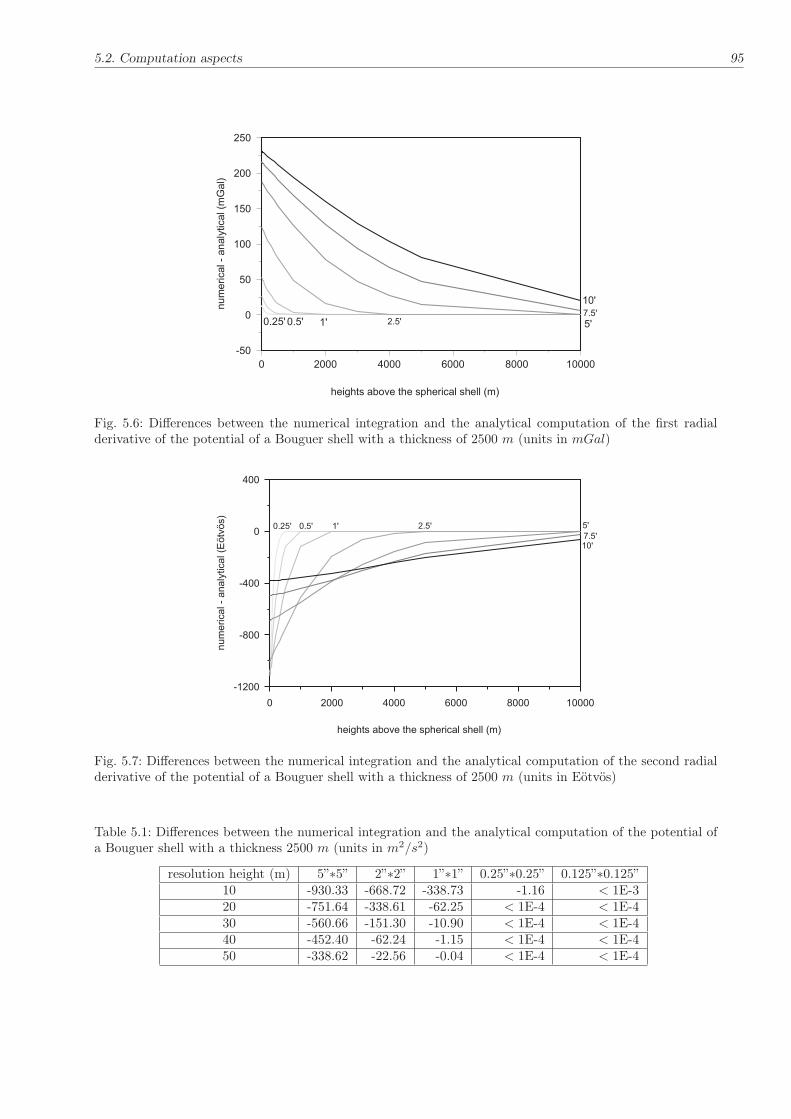
5.2. Computation aspects 95
0 2000 4000 6000 8000 10000
heights above the spherical shell (m)
-50
0
50
100
150
200
250
nu
me
rical-
an
aly
tical(m
Gal)
10'
5'0.5' 2.5'1'7.5'
0.25'
Fig. 5.6: Differences between the numerical integration and the analytical computation of the first radialderivative of the potential of a Bouguer shell with a thickness of 2500 m (units in mGal)
0 2000 4000 6000 8000 10000
heights above the spherical shell (m)
-1200
-800
-400
0
400
num
erica
l-
ana
lytica
l(E
ötv
ös)
2.5'
10'7.5'
5'0.5'0.25' 1'
Fig. 5.7: Differences between the numerical integration and the analytical computation of the second radialderivative of the potential of a Bouguer shell with a thickness of 2500 m (units in Eötvös)
Table 5.1: Differences between the numerical integration and the analytical computation of the potential ofa Bouguer shell with a thickness 2500 m (units in m2/s2)
resolution height (m) 5”∗5” 2”∗2” 1”∗1” 0.25”∗0.25” 0.125”∗0.125”10 -930.33 -668.72 -338.73 -1.16 < 1E-320 -751.64 -338.61 -62.25 < 1E-4 < 1E-430 -560.66 -151.30 -10.90 < 1E-4 < 1E-440 -452.40 -62.24 -1.15 < 1E-4 < 1E-450 -338.62 -22.56 -0.04 < 1E-4 < 1E-4

96 5. Numerical analysis
and an inner limit of
∂2Vt−∂r2
∣∣∣∣r=R2
= −4πGρ
3R32
(R3
2 + 2R31
). (5.5)
We cannot expect a reasonable result in case of computation points close to or at the outer spherical surfaceof the shell.
The numerical values for the present example read for the outer limit of the radial component 1.75 Eötvösand for the inner limit −2236 Eötvös. The results of the numerical integration for computation points at thesurface of the shell turn out to be (approximately) the arithmetic mean of the inner and the outer values,approximately −1118 Eötvös (Fig. 5.9). This is only the case if the resolution is selected adequately high -in case of a coarse grid the approximation errors cannot be interpreted anymore. The situation cannot beexplained in such a simple way as in case of the local horizontal directions x and y which are perpendicularto the radial direction. No jump occurs in these cases, so that it holds at the outer shell boundary, e.g., forthe derivation with respect to x,
∂2Vt+∂x2
∣∣∣∣r=R2
=∂2Vt−∂x2
∣∣∣∣r=R2
. (5.6)
Therefore, in these cases there would be no reason for an unstable behavior as in case of the radial component.Here we have to keep in mind that the formulae for the computation of the second derivatives are derived suchthat the Laplace equation is fulfilled in the space outside the masses as demonstrated in Figs. 5.7 and 5.8,even if the computation point is arbitrarily close to the surface of the shell. This is the case despite the factthat the formulae are only approximate. A numerical consequence is that the second horizontal derivativeswill never converge to the correct value at the outer boundary even in case of a very fine resolution of thedigital terrain model (Fig. 5.9).
In the vicinity of the computation point a rigorous tesseroid formula in three dimensions (Kuhn 2000a) isnecessary or to choose a sufficient fine grid of the DTM, where a planar approximation based on the prismformulae technique of Nagy (1966) might be sufficient. It should be pointed out that the Laplace equationis fulfilled as long as the computation point is located outside the masses as demonstrated in Figs. 5.7 and5.8, even if the computation point is arbitrarily close to the surface of the shell. The situation is less criticalin practical applications as it may seem from the aforementioned facts; in these cases a Bouguer plate ora Bouguer shell is used, whose effects can be determined analytically, and the (in general small) terraincorrections can be determined by numerical integration based on a DTM with a sufficient fine resolutionor any rigorous (planar) formula. A detailed investigation of these error effects has to be performed in aforthcoming study.
5.2.2 Surface spherical harmonic expansion of the topography
There are many methods for calculating the surface spherical harmonic expansions of the topography suchas quadrature methods, least squares, Paul integral, integral through Legendre polynomials (see, e.g., Tsoulis1999a; Sneeuw 1994; Sneeuw and Bun 1996). In this investigation only a simple quadrature and the Gauss-Legendre quadrature methods have been used.
5.2.2.1 Resolution aspects
The spherical harmonic expansion of the topography is a very efficient technique for calculating thetopographic-isostatic mass effects, but it is limited to an upper spherical harmonic degree of about 2700which corresponds to a 4 arc-minute resolution. Beyond this degree numerical computation problems con-cerning the stability of the recursive computation of the associated Legendre’s functions occur (see, e.g.,Holmes and Featherstone 2002) and increasing the computational time. For this reason, the spherical har-monic expansion of the topography can be used for calculating the long and medium wavelength effects ofthe topography. These long and medium wavelengths are important for calculating the effects at satellitealtitude or for calculating the far-zone effects of the topographic masses for the points at the Earth’s surfaceand at certain altitudes for airborne gravimetry.
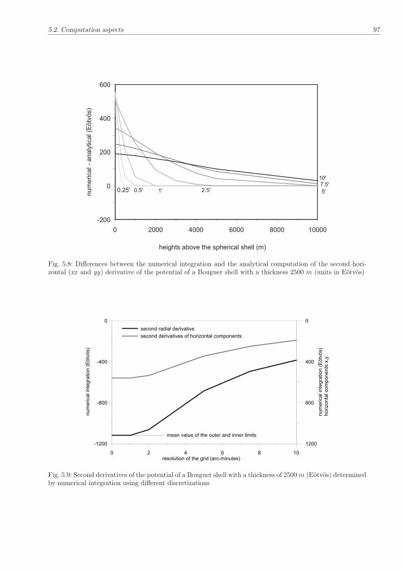
5.2. Computation aspects 97
0 2000 4000 6000 8000 10000
heights above the spherical shell (m)
-200
0
200
400
600num
erica
l-
analy
tical(E
ötv
ös)
10'
2.5' 5'1'0.5'7.5'
0.25'
Fig. 5.8: Differences between the numerical integration and the analytical computation of the second hori-zontal (xx and yy) derivative of the potential of a Bouguer shell with a thickness 2500 m (units in Eötvös)
0 2 4 6 8 10resolution of the grid (arc-minutes)
-1200
-800
-400
0
numerical integration (Eötvös)
second radial derivative
second derivatives of horizontal components
1200
800
400
0numerical integration (Eötvös)
horizontal components x,y
mean value of the outer and inner limits
Fig. 5.9: Second derivatives of the potential of a Bouguer shell with a thickness of 2500m (Eötvös) determinedby numerical integration using different discretizations

98 5. Numerical analysis
5.2.2.2 Numerical computation of the surface spherical harmonics
It is known that a square integrable function on the sphere can be developed into harmonic coefficients usingthe global spherical harmonic analysis (GSHA). In our study, the integrable function is the topography abovethe geoid. The computation of the spherical harmonics using quadrature method will be discussed in thefollowing.
Simple quadrature method The spherical harmonic coefficients of the topography can be calculated byreplacing the double integral by a double summation all over the world. For an efficient computation, thetwo step analysis approach proposed by Neumann (1838) and Gauss (1839) has been applied. The doubleintegration or summation is splitted into a longitude and a latitude dependent part. For example, Eq. (4.134)reads as follows (e.g. in case of k=1):
hkαnm =1
4π
∫∫
σ
(Heq(ϕ, λ)
R
)
Y αnmdσ. (5.7)
This equation can be splitted into two equations as follows:
{
am(ϕ)
bm(ϕ)
}
=1
(1 + δm0)π
2π∫
λ=0
(Heq(ϕ, λ)
R
){
cosmλ
sinmλ
}
dλ, (5.8)
{
hcnm
hsnm
}
=1
4(1 + δm0)
π∫
ϕ=0
{
am(ϕ)
bm(ϕ)
}
Pnm(sinϕ) cosϕdϕ. (5.9)
The reason for the greater efficiency of the two-step formulation is twofold. Firstly, Eq. (5.8) can be treated byFourier transformations over single parallels. Secondly, the equations may be evaluated for separate ordersm. In reality one has to deal with discretized function values, either point values or area means. In ourstudy, we approximate the function of heights by point values. The aliasing problem will be ignored, i.e. it isassumed that the function does not contain information above degree N . Since the distribution of parallelshas not been decided yet and since the problem of non-orthogonality of the discretized Legendre functionhas not been resolved, the determination of coefficients is still bending. In order to solve this problem ofnon-orthogonality, Neumann’s method has been used.
Neumann’s method A special case of exact quadrature is achieved by restricting the ϕ-grid. Neumann(1887) showed that if one chooses the latitude circles to coincide with the zeros of the Legendre polynomialsof degree N + 1, i.e.
PNmax+1(sinϕi) = 0, i = 1, 2, ..., Nmax, (5.10)
the number of parallels can be reduced to N = Nmax + 1. The specific ϕ- or ϑ-grid leads to the Gauss-Legendre quadrature method (Lanczos 1956; Krylov 1962; Stroud and Secrest 1966; Colombo 1981). Thespecific grid is referred as Gauss grid (Payne 1971). Neumann’s method can be summarized as follows: Anexact GSHA is performed up to degree Nmax making use of a Gauss-Neumann grid (see Fig. 5.10 blue),defined by:
PNmax+1(sinϕi) = 0, i = 1, 2, ..., Nmax + 1,
λj = j∆λ, j = 1, 2, ..., 2Nmax − 1,
∆λ =π
Nmax.
(5.11)
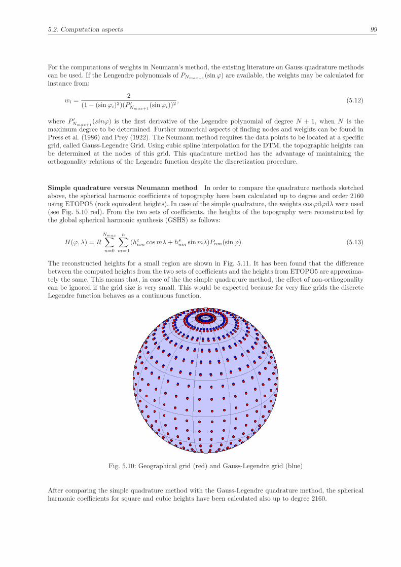
5.2. Computation aspects 99
For the computations of weights in Neumann’s method, the existing literature on Gauss quadrature methodscan be used. If the Lengendre polynomials of PNmax+1
(sinϕ) are available, the weights may be calculated forinstance from:
wi =2
(1 − (sinϕi)2)(P ′
Nmax+1(sinϕi))2
, (5.12)
where P ′
Nmax+1(sinϕ) is the first derivative of the Legendre polynomial of degree N + 1, when N is the
maximum degree to be determined. Further numerical aspects of finding nodes and weights can be found inPress et al. (1986) and Prey (1922). The Neumann method requires the data points to be located at a specificgrid, called Gauss-Legendre Grid. Using cubic spline interpolation for the DTM, the topographic heights canbe determined at the nodes of this grid. This quadrature method has the advantage of maintaining theorthogonality relations of the Legendre function despite the discretization procedure.
Simple quadrature versus Neumann method In order to compare the quadrature methods sketchedabove, the spherical harmonic coefficients of topography have been calculated up to degree and order 2160using ETOPO5 (rock equivalent heights). In case of the simple quadrature, the weights cosϕdϕdλ were used(see Fig. 5.10 red). From the two sets of coefficients, the heights of the topography were reconstructed bythe global spherical harmonic synthesis (GSHS) as follows:
H(ϕ, λ) = R
Nmax∑
n=0
n∑
m=0
(hcnm cosmλ+ hsnm sinmλ)Pnm(sinϕ). (5.13)
The reconstructed heights for a small region are shown in Fig. 5.11. It has been found that the differencebetween the computed heights from the two sets of coefficients and the heights from ETOPO5 are approxima-tely the same. This means that, in case of the the simple quadrature method, the effect of non-orthogonalitycan be ignored if the grid size is very small. This would be expected because for very fine grids the discreteLegendre function behaves as a continuous function.
Fig. 5.10: Geographical grid (red) and Gauss-Legendre grid (blue)
After comparing the simple quadrature method with the Gauss-Legendre quadrature method, the sphericalharmonic coefficients for square and cubic heights have been calculated also up to degree 2160.

100 5. Numerical analysis
108.5 109 109.5
35.5
36
36.5
-14
-12
-10
-8
-6
-4
-2
0
2
4
6
8
10
12
14
108.5 109 109.5
35.5
36
36.5
-14
-12
-10
-8
-6
-4
-2
0
2
4
6
8
10
12
14
108.5 109 109.5
35.5
36
36.5
600
700
800
900
1000
1100
1200
1300
1400
1500
ETOPO5 - topography from simple quadrature
ETOPO5 - topography from Gauss quadrature
ETOPO5 topography
108.5 109 109.5
35.5
36
36.5
600
700
800
900
1000
1100
1200
1300
1400
1500
108.5 109 109.5
35.5
36
36.5
600
700
800
900
1000
1100
1200
1300
1400
1500
topography from Gauss quadrature coefficients
topography from simple quadrature coefficients
Fig. 5.11: Comparison between simple quadrature and Gauss Legendre quadrature methods (units in meter)
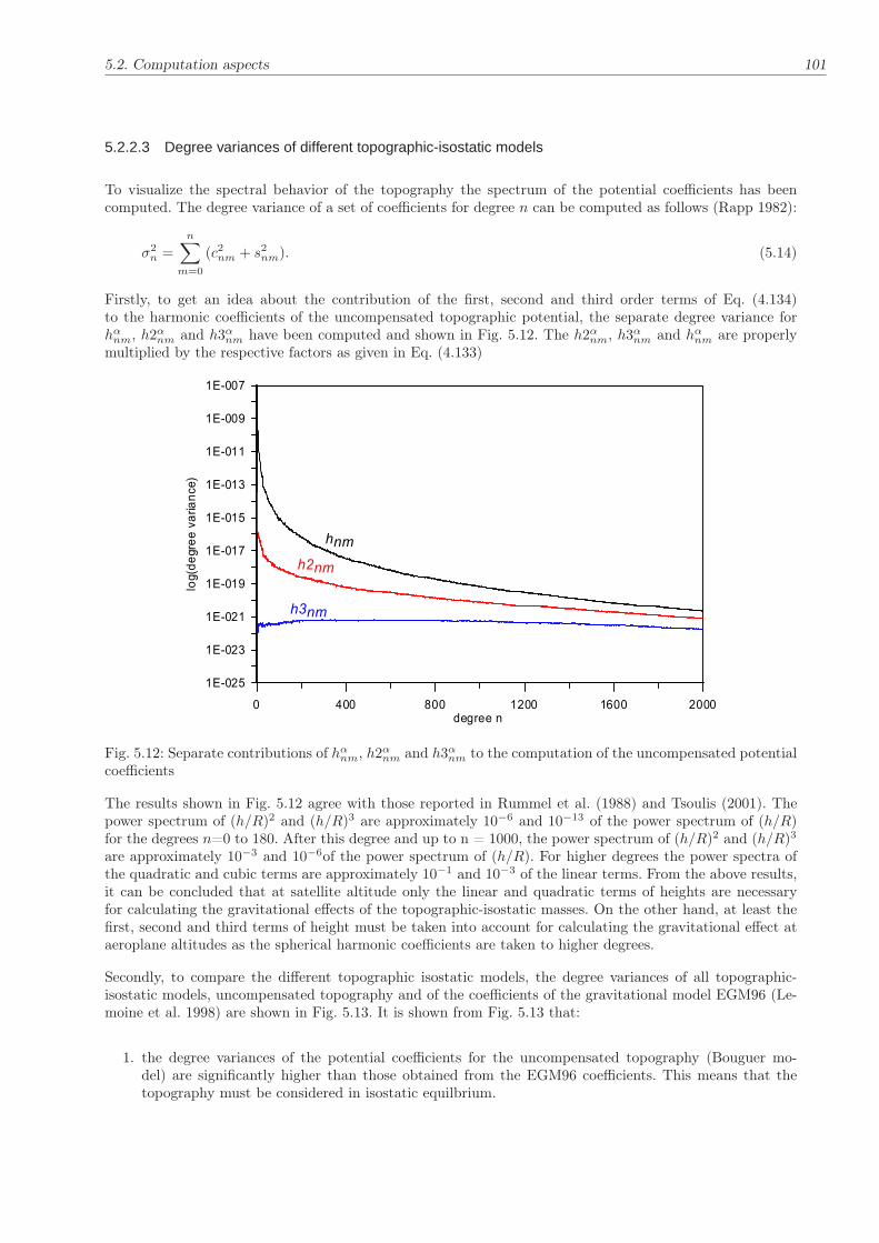
5.2. Computation aspects 101
5.2.2.3 Degree variances of different topographic-isostatic models
To visualize the spectral behavior of the topography the spectrum of the potential coefficients has beencomputed. The degree variance of a set of coefficients for degree n can be computed as follows (Rapp 1982):
σ2n =
n∑
m=0
(c2nm + s2nm). (5.14)
Firstly, to get an idea about the contribution of the first, second and third order terms of Eq. (4.134)to the harmonic coefficients of the uncompensated topographic potential, the separate degree variance forhαnm, h2αnm and h3αnm have been computed and shown in Fig. 5.12. The h2αnm, h3αnm and hαnm are properlymultiplied by the respective factors as given in Eq. (4.133)
0 400 800 1200 1600 2000degree n
1E-025
1E-023
1E-021
1E-019
1E-017
1E-015
1E-013
1E-011
1E-009
1E-007
log(degree variance)
hnm
h2nm
h3nm
Fig. 5.12: Separate contributions of hαnm, h2αnm and h3αnm to the computation of the uncompensated potentialcoefficients
The results shown in Fig. 5.12 agree with those reported in Rummel et al. (1988) and Tsoulis (2001). Thepower spectrum of (h/R)2 and (h/R)3 are approximately 10−6 and 10−13 of the power spectrum of (h/R)for the degrees n=0 to 180. After this degree and up to n = 1000, the power spectrum of (h/R)2 and (h/R)3
are approximately 10−3 and 10−6of the power spectrum of (h/R). For higher degrees the power spectra ofthe quadratic and cubic terms are approximately 10−1 and 10−3 of the linear terms. From the above results,it can be concluded that at satellite altitude only the linear and quadratic terms of heights are necessaryfor calculating the gravitational effects of the topographic-isostatic masses. On the other hand, at least thefirst, second and third terms of height must be taken into account for calculating the gravitational effect ataeroplane altitudes as the spherical harmonic coefficients are taken to higher degrees.
Secondly, to compare the different topographic isostatic models, the degree variances of all topographic-isostatic models, uncompensated topography and of the coefficients of the gravitational model EGM96 (Le-moine et al. 1998) are shown in Fig. 5.13. It is shown from Fig. 5.13 that:
1. the degree variances of the potential coefficients for the uncompensated topography (Bouguer mo-del) are significantly higher than those obtained from the EGM96 coefficients. This means that thetopography must be considered in isostatic equilbrium.

102 5. Numerical analysis
0 400 800 1200 1600 2000
degree n
1E-027
1E-022
1E-017
1E-012
log (degree variance)
EGM96
uncompensated topography
Airy-Heiskanen model
Vening Meinesz model
generalized Helmert (D1=32 km)
Helmert's second method
Pratt-Hayford model
combined Airy and Pratt
Fig. 5.13: Degree variances of different topographic-isostatic models
2. the degree variances of the potential coefficients of the Airy-Heiskanen model and the generalizedHelmert’s model of condensation with a condensation depth=32 km are approximately the same.
3. the degree variances of the Pratt-Hayford model are approximately the same as for the combined Airyand Pratt model. This means that the effects of the topographic heights are significantly smaller thanthe effects of bathymetric heights.
4. the degree variances of the Pratt-Hayford model agree quit well with the degree variance of the EGM96coefficients.
5. the degree variances of the Vening Meinesz model are larger than the degree variances of the Airy-Heiskanen model for high degrees. This is caused by smoothing the roots and anti-roots in case of theVening Meinesz model.
5.2.3 Near-zone and far-zone aspects
The effects of topographic-isostatic masses must be calculated globally which is very expensive in terms ofcomputation time. To overcome this problem, the surface integration domain is divided into two integrationsub-domains: a spherical cap around the computation point with a small radius, called near-zone contribution(σ0), and the rest of the Earth, called far-zone contribution (σFz). A fine resolution DTM must be used inthe near zone while in the far-zone a coarser DTM is sufficient in most cases (Grüninger 1990). Near-zonetopographic effects on the gravity and geoid heights can be calculated using rectangular prisms (Nagy 1966;Nagy et al. 2000, 2002), which lead to a particularly simple formula, or by using tesseroid formulae in case ofthe spherical approximation of the geoid (Smith et al. 2001; Kuhn and Seitz 2005; Makhloof and Ilk 2006). Toarrive at economic computation formulae, the far-zone effects are represented by a global spherical harmonicexpansion of the topography. This can be performed by a Molodenskii-type spectral approach as shown inchapter 4.

5.3. Effects of topographic-isostatic masses at the surface of the Earth and at aeroplane altitudes 103
5.3 Effects of topographic-isostatic masses at the surface of the Earthand at aeroplane altitudes
In this section the near and far-zone effects of the topography will be discussed at the surface of the Earth andat aeroplane altitude. The potential of the topographic-isoatatic masses in terms of the indirect topographicaleffect has been computed. Also, the first derivatives of the potential in terms of the direct topographical effecthave been determined. Moreover, the second derivatives of the potential of the topographic-isotatic massesat aeroplane altitude have been studied numerically.
5.3.1 Near-zone topography effects
To give an impression of the size and distribution of the topographic-isostatic mass effects on the gravitatio-nal functionals at the Earth’s surface and at aeroplane altitudes, the Airy-Heiskanen model and Helmert’smethods of condensation have been used. To reduce the discretization errors, the direct and indirect topo-graphical effects have been splitted into two effects: (1) the effects of the Bouguer shells and (2) the effectsof the terrain refinements. As the effects of the Bouguer shells of topographic and isostatic masses canceleach other in case of the direct topographical effect, only the terrain effects have been computed. In case ofthe primary indirect topographical effect, the terrain effects in addition to the effects of the Bouguer shellshave been determined.
5.3.1.1 Direct terrain effect on gravity
In order to take the short wavelengths of the topography into account, the near-zone cap has been takento be ψ0 = 30. For the generalized Helmert model of condensation the depth of the condensation masseshas been varied between 21 km to 40 km. These tests have been performed to show the coincidence ofHelmert’s models with an an appropriate condensation depth with the Airy-Heiskanen isostatic model. Thecomputation points has an altitude of 4 km above the sea level. Examples of Helmert’s generalized modelswith condensation depths (21, 25, 30, 32, 35 and 40 km) together with the Airy-Heiskanen model are givenin Table 5.2.
Table 5.2: Near-zone terrain effects at an altitude of 4 km for Helmert’s first and generalized model ofcondensation with different depths in comparison with Airy-Heiskanen (units in mGal)
topographic-isostatic model RMS Mean Min MaxHelmert’s first method (21 km) 23.78 -4.23 -67.90 56.99generalized Helmert model (25 km) 24.13 -4.76 -69.47 57.12generalized Helmert model (30 km) 24.32 -5.45 -70.60 56.60generalized Helmert model (32 km) 24.32 -5.58 -70.86 56.25Airy-Heiskanen model 24.32 -6.04 -70.46 55.79generalized Helmert model (35 km) 24.31 -5.89 -71.09 55.61generalized Helmert model (40 km) 24.20 -6.38 -71.13 54.35
The coincidence of the generalized Helmert model of condensation with the Airy-Heiskanen model depends onthe condensation depths of Helmert’s model (Table 5.2). This means that, with a proper selection of Helmert’scondensation depth D1, the condensation method can be adjusted to be more realistic. To illustrate the sizeof the direct terrain effect dependent on the height of the calculation points, the direct terrain effects at thealtitudes of 4 km, 6 km, 8 km, 10 km are shown in Table 5.3
Finally, to give an impression about the distribution of the near-zone terrain effects, the direct terrain effectfor Helmert’s second method of condensation, Helmert’s generalized model with a condensation depth of 32km and Airy-Heiskanen method are shown in Fig. 5.14.

104 5. Numerical analysis
241.5 242.0 242.5 243.0 243.5
49.5
50.0
50.5
51.0
51.5
-14
-10
-6
-2
2
6
10
14
Helmert's second method of condensation(Max=15.83, Min=-30.17, Mean=- 0.45, RMS=6.97)
Airy-Heiskanen model(Max=55.79, Min=-70.46, Mean=-6.01, RMS=24.31)
generalized Helmert model of condensation( w ith condensation depth =32 km ;Max=56.25, Min=-70.86, Mean=-5.58, RMS=24.32)
241.5 242.0 242.5 243.0 243.5
49.5
50.0
50.5
51.0
51.5
-70
-60
-50
-40
-30
-20
-10
0
10
20
30
40
50
241.5 242.0 242.5 243.0 243.5
49.5
50.0
50.5
51.0
51.5
-70
-60
-50
-40
-30
-20
-10
0
10
20
30
40
50
Fig. 5.14: Near-zone direct terrain effect on gravity of the area inside a cap size of ψ0 = 30 for differenttopographic-isostatic models at an altitude of 4 km (units in mGal)

5.3. Effects of topographic-isostatic masses at the surface of the Earth and at aeroplane altitudes 105
5.3.1.2 Indirect topographical effect on geoid and gravity
It is shown in Eq. (4.202) that the primary indirect topographical effects includes two parts: the effects of theBouguer shells of the topographic and isostatic masses and the terrain effects. The effects of the Bouguer shellof the topographic masses and the Bouguer layer of the condensation masses in case of Helmert’s methodsof condensation can be determined by the following equation:
PITEBouguer =2πGρcr
[(R+HP ′)2 −R2
]
γ0− 4πGρcr
3(R+HP ′)γ0
[(R+HP ′)3 −R3)
], (5.15)
where HP ′ is the orthometric height of the topography at the computation point. It can be seen that Eq.(5.15) is independent of the condensation depth of Helmert’s first or generalized model of condensation.This is due to the fact that the potentials of the Bouguer layers of the condensation masses in case ofHelmert’s first and second method of condensation are equal. Also, the potential of the Bouguer shell of thecompensating masses in case of the Airy-Heiskanen model are equal to the potential of the Bouguer layer incase of Helmert’s model. This is based on the mass conservation principle of the topographic and isostaticor condensation masses. The effects of the Bouguer shells for the Canadian Rocky Mountains are shown inFig. 5.15.Also, the near-zone primary indirect terrain effects are shown in Fig. 5.16. The plot shows that the primary
241.5 242 242.5 243 243.5
49.5
50
50.5
51
51.5
-0.9
-0.8
-0.7
-0.6
-0.5
-0.4
-0.3
-0.2
-0.1
Fig. 5.15: Primary indirect effects of Bouguer shells of the topographic masses (units in mGal)
indirect terrain effects in case of the generalized Helmert model of condensation and the Airy-Heiskanenmodel are large compared to the effects of the Bouguer shells and depend significantly on the heights ofthe topography. These effects must be taken into account for calculating the 1 cm geoid in case of localgeoid determination. On the other hand the near zone primary indirect terrain effects in case of Helmert’ssecond method of condensation are small but these value must be taken into account in case of 1 cm geoiddetermination. Finally, the near zone secondary indirect terrain effects for the same area are shown in Fig.5.17. Again the near-zone secondary indirect terrain effects for Helmert’s first and the generalized methodsas well as Airy-Heiskanen method reach significant values compared to the accuracy of the observation data.
5.3.1.3 Terrain effect on airborne gradiometry
Airborne gravity gradiometry is not yet popular but may represent a potential technique for the future, e.g.,it is imaginable that HALO (High Altitude and LOng Range Research Aircraft) could be equipped with

106 5. Numerical analysis
241.5 242.0 242.5 243.0 243.5
49.5
50.0
50.5
51.0
51.5
-0.04
-0.02
0.00
0.02
0.04
0.06
0.08
0.10
Helmert's second method of condensation(Max=0.11, Min=-0.06, Mean=0.02, RMS=0.023)
Airy-Heiskanen model(Max=3.62, M in=-4.52, Mean=-0.15, RMS=1.44)
generalized Helmert model of condensation(w ith condensation depth =32 km;Max=3.23, Min=-3.65, Mean=-0.12, RMS=1.23)
241.5 242.0 242.5 243.0 243.5
49.5
50.0
50.5
51.0
51.5
-3.50
-2.50
-1.50
-0.50
0.50
1.50
2.50
3.50
241.5 242.0 242.5 243.0 243.5
49.5
50.0
50.5
51.0
51.5
-3.50
-2.50
-1.50
-0.50
0.50
1.50
2.50
3.50
Fig. 5.16: Near-zone primary indirect terrain effect on geoid heights of the area inside a cap size of ψ0 = 30
for different topographic-compensation models (units in meter)

5.3. Effects of topographic-isostatic masses at the surface of the Earth and at aeroplane altitudes 107
241.5 242.0 242.5 243.0 243.5
49.5
50.0
50.5
51.0
51.5
-0.04
-0.03
-0.02
-0.01
0.00
0.01
0.02
Helmert's second method of condensation(Max=0.012, Min=-0.037, Mean=-0.002, RMS=0.006)
Airy-Heiskanen model(Max=1.14, Min=-1.52, Mean=-0.06, RMS=0.47)
generalized Helmert model of condensation( with condensation depth =32 km;Max=1.02, Min=-1.26, Mean=-0.05, RMS=0.40)
241.5 242.0 242.5 243.0 243.5
49.5
50.0
50.5
51.0
51.5
-1.20
-1.00
-0.80
-0.60
-0.40
-0.20
-0.00
0.20
0.40
0.60
0.80
1.00
241.5 242.0 242.5 243.0 243.5
49.5
50.0
50.5
51.0
51.5
-1.20
-1.00
-0.80
-0.60
-0.40
-0.20
-0.00
0.20
0.40
0.60
0.80
1.00
Fig. 5.17: Near-zone secondary indirect terrain effect on gravity of the area inside a cap size of ψ0 = 30 fordifferent topographic-isostatic models at the surface of the Earth (units in mGal)

108 5. Numerical analysis
a gravity gradiometer. Therefore, it is interesting to investigate the topographic-isostatic effects of gravitygradients in an aeroplane altitude. The near-zone terrain effects of the topographic-isostatic masses on thegravitational tensor component Vzz at an altitude of 10 km based on the Airy-Heiskanen model is shown inFig. 5.18 for the Himalaya region.
75 80 85 90 95 100
30
35
40
-80
-60
-40
-20
0
20
40
60
80
Fig. 5.18: Effects of the near-zone terrain masses on the tensor component Vzz at an altitude of 10 km forthe Airy-Heiskanen model for the Himalaya region (units in Eötvös)
5.3.2 Far-zone topography effects
The computational area is taken as the same used for the near-zone terrain effects (Fig. 5.1). The calculationsare performed for a far-zone cap size of ψ0 ≥ 30. In this case the series expansions fulfill the convergencecriterion given in Eq. (A.6). In addition, various other cases of far zones have been investigated. The upperdegree of the spherical harmonic expansion of the topography is taken to be Nmax = 360 as the effects abovethis degree are neglected (will be seen later). Again, for the generalized Helmert model of condensation thedepth of the condensation masses has been varied between 21 km to 40 km. These tests have been performedto show that a varying condensation depth approximates the Airy-Heiskanen isostatic model quite well.Examples of condensation depths (21, 25, 30, 32, 35 and 40 km) are given in Table 5.4.
5.3.2.1 Direct terrain effect on gravity
To illustrate the size of the direct terrain effect against the cap size of the far-zone, the RMS-values (rootmean square of point values) of these effects for the three models are shown in Fig. 5.19 for computationpoints at an altitude of 4 km. It is shown that a far-zone cap size of ψ0 ≥ 30 gives small RMS-values incase of Helmert’s second method of condensation compared to the accuracy of the observation. Table 5.5shows the far-zone effects in case of cap-size radii of 30, 100 and 200 in case of Helmert’s second method ofcondensation. The situation is different in case of the generalized Helmert model of condensation and theAiry-Heiskanen model where these effects are much larger. Table 5.6 gives an overview of the far-zone effectsdepending on the cap-size radius (30, 100, 200,......,900). It is interesting to note that these effects dependonly marginally on the altitude of the computation points.
The accuracy of the spherical harmonic formulae derived in this case has been tested using the integrationmethod with tesseroid formulae (Makhloof and Ilk 2006). Figure 5.20 shows the direct terrain far-zone effectsalong the 500 latitude, determined by the formulae based on a spherical harmonic expansion up to degreeNmax = 360 and based on a numerical quadrature method using tesseroid formulae with a corresponding grid

5.3. Effects of topographic-isostatic masses at the surface of the Earth and at aeroplane altitudes 109
Table 5.3: Near-zone direct terrain effects for different altitudes for Helmert’s methods of condensation andAiry-Heiskanen model (units in mGal)
Model statistics H= 4 km H= 6 km H= 8 km H= 10 km
Helmert’s second method
RMS 6.97 3.93 2.63 1.91Max 15.83 9.42 6.46 4.54Min -30.17 -13.17 -8.24 -5.81Mean -0.45 -0.35 -0.31 -0.28
generalized Helmert (D1=32 km)
RMS 24.32 18.07 14.42 12.02Max 56.25 37.62 30.24 25.30Min -70.86 -49.49 -45.33 -41.62Mean -5.58 -5.19 -4.92 -4.69
Airy-Heiskanen model
RMS 24.31 18.21 14.67 12.37Max 55.79 37.07 30.49 25.64Min -70.46 -51.87 -48.46 -44.50Mean -6.01 -5.65 -5.36 -5.11
0 10 20 30 40spherical distance
0
10
20
30
RM
S (
mG
al)
Airy-Heiskanen model
Helmert's second method of condensation
generalized Helmert model (D1 =32 km)
Fig. 5.19: RMS of direct topographical effects at an altitude of 4 km against the cap radius for differenttopographic-isostatic models
Table 5.4: Far-zone terrain effects at an altitude of 4 km for Helmert’s first and generalized model of con-densation with different depths in comparison with Airy-Heiskanen (units in mGal)
topographic-isostatic model RMS Mean Min MaxHelmert’s first method (21 km) 3.25 -8.49 -16.21 -0.31generalized Helmert model (25 km) 3.82 -10.08 -19.13 -0.43generalized Helmert model (30 km) 4.53 -12.07 -22.77 -0.58generalized Helmert model (32 km) 4.82 -12.86 -24.23 -0.65Airy-Heiskanen model 5.58 -13.05 -26.88 0.44generalized Helmert model (35 km) 5.25 -14.05 -26.41 -0.74generalized Helmert model (40 km) 5.95 -16.03 -30.03 -0.91

110 5. Numerical analysis
Table 5.5: Far-zone direct terrain effects for different cap size radii and different altitudes in case of Helmert’ssecond method of condensation (units in mGal)
cap radius statistics Earth surface H= 4 km H= 6 km H= 10 km
30
RMS 0.238 0.237 0.237 0.234Max 0.301 0.301 0.301 0.300Min -0.844 -0.843 -0.840 -0.828Mean -0.131 -0.129 -0.128 -0.122
100
RMS 0.071 0.071 0.070 0.070Max 0.164 0.164 0.165 0.166Min -0.177 -0.176 -0.175 -0.171Mean 0.035 0.036 0.037 0.039
200
RMS 0.033 0.033 0.034 0.034Max 0.103 0.103 0.103 0.103Min -0.059 -0.059 -0.058 -0.056Mean 0.042 0.042 0.042 0.044
Table 5.6: Far-zone direct terrain effects for different cap size radii and different altitudes in case of thegeneralized Helmert model of condensation (D1 = 32 km; units in mGal)
cap radius statistics Earth surface H= 4 km H= 6 km H= 10 km
30
RMS 4.835 4.820 4.812 4.803Max -0.631 -0.640 -0.650 -0.660Min -24.285 -24.230 -24.220 -24.149Mean -12.900 -12.860 -12.850 -12.828
100
RMS 1.418 1.418 1.417 1.415Max -3.620 -3.615 -3.614 -3.609Min -10.596 -10.590 -10.580 -10.560Mean -7.344 -7.338 -7.330 -7.323
200
RMS 0.716 0.716 0.715 0.714Max 2.647 -2.645 -2.643 -2.639Min -6.181 -6.181 -6.178 -6.170Mean -4.514 -4.513 -4.511 -4.505
400
RMS 0.336 0.335 0.335 0.335Max -1.414 -1.413 -1.412 -1.410Min -3.068 -3.067 -3.065 -3.061Mean -2.277 -2.76 -2.275 -2.272
500
RMS 0.251 0.251 0.251 0.250Max -1.008 -1.007 -1.006 -1.005Min -2.242 -2.241 -2.240 -2.238Mean -1.653 -1.652 -1.651 -1.649
900
RMS 0.093 0.093 0.093 0.093Max -0.330 -0.329 -0.329 -0.329Min -0.785 -0.785 -0.784 -0.784Mean -0.565 -0.564 -0.564 -0.564

5.3. Effects of topographic-isostatic masses at the surface of the Earth and at aeroplane altitudes 111
size of 5′∗5′. There are identical results in case of Helmert’s condensation methods and some small differencesin case of the Airy-Heiskanen method. These differences most probably are caused by the restriction of theTaylor expansions of Eq. (A.4) and Eq. (A.9) to the second term only. For this reason it would be necessaryto develop the series including the cubic term of Taylor expansions for distance and logarithmic functions toremove these differences. Another interesting aspect of this method is the choice of the maximum expansiondegree of the spherical harmonic series representing the topography. Figure 5.21 gives an impression of thesize of different spectral bands of the spherical harmonic expansion. It seems that an upper degree of 100 issufficient even for high accuracy airborne gravimetry (1-2 mGal) for all topographic-compensation modelsinvestigated here. At the Earth’s surface a high degree of Nmax = 360 is necessary to consider the effects ofthe topographic-compensating masses in case of Helmert’s first or generalized methods of condensation andthe Airy-Heiskanen isostatic model. In case of Helmert’s second method of condensation, an upper degree of50 may fulfill the accuracy demand of Earth’s surface gravimetry.
To give an impression of the distribution of the far-zone terrain effects depending on the topography withinthe near zone, the direct terrain effect for Helmert’s methods of condensation and the Airy-Heiskanen modelat an altitude of 4 km are plotted in Fig. 5.22.
5.3.2.2 Indirect terrain effect on geoid and gravity
Finally, the indirect terrain effects for the same test region are shown in Figs. 5.24 and 5.25. Figure 5.24 showsthe far-zone primary indirect terrain effects on the geoid heights for the different topographic-compensatingmodels. The effects are rather large for the generalized Helmert model (D1 = 32 km) and for the Airy-Heiskanen model, except those for Helmert’s second condensation method. The situation is similar for thefar-zone secondary indirect terrain effects on gravity at the surface of the Earth as Fig. 5.25 demonstrates.
5.3.2.3 Concluding remarks to the terrain effects of gravity and geoid heights
For the cap size of ψ0 = 30 investigated here, the far-zone contributions for the primary topographic indirecteffect are as large as up to 13 m while the direct topographic effect is in the size of up to 28 mGal. Thatmeans that the far-zone contributions to the primary indirect effects are of comparable magnitude as thenear-zone contributions in contrast to the direct effect. This is caused by the fact that the potential is inverseto the distance between the computation point and mass elements while gravity is inverse to the squareddistance which tapers off more quickly.
From Fig. 5.22 it can be concluded that the far-zone terrain effects at aeroplane altitude in case of Helmert’ssecond method of condensation can be neglected for spherical cap size radii larger than 30 as the maximumvalues of these effects are smaller than the accuracy of the airborne gravity measurements (1-2 mGal). On theother hand, these effects must be taken into account for Helmert’s first or generalized model of condensationand the Airy-Heiskanen model. Figure 5.23 shows that the far-zone effects at the surface of the Earth aremore or less the same as at aeroplane attitudes higher than 4 km and for all topographic-isostatic models.
The results of the far-zone effects determined in the present investigation at the surface of the Earth werecompared with those calculated from Novàk et al. (2001). Both soluations are shown in Fig. 5.26. Thereare some differences between the two methods. These differences are caused by a different handling of thetopography height of the computation point. In case of Novàk et al. (2001) the heights of the computationpoints are computed from the spherical harmonic expansion up to the maximum degree used for calculatingthe far-zone effects. This is not sufficient for a precise determination of the far-zone effects. But we have topoint out that this holds for a region with a rough topography. Therefore the differences between the twomethods may be neglected for areas with a smooth topography or if the maximum degree of the sphericalharmonic expansion of the topography has been extended to a high degree as for example Nmax = 2160.
The formulae based on the spherical harmonics as derived in this study are very efficient. The computationof the various topographic-isostatic effects at a grid with a grid size of 5′ ∗ 5′ – these are 1296 point values

112 5. Numerical analysis
242 243longitude (degree)
-25
-20
-15
-10
-5
0
dir
ect
te
rra
in e
ffe
ct (
mG
al)
Airy-Heiskanen model spherical harmonic expansion
direct integration method
242 243longitude (degree)
-24
-20
-16
-12
-8
-4
0
dir
ect
ter
rain
eff
ec
t (m
Ga
l)
generalized Helmert method of condensation ( D1 = 32 km)
spherical harmonic expansion
direct integration method
242 243longitude (degree)
-0.7
-0.6
-0.5
-0.4
-0.3
-0.2
-0.1
0
0.1
0.2
0.3d
ire
ct t
err
ain
eff
ect
(m
Ga
l)
Helmert 's second method of condensation
spherical harmonic expansion
direct integration method
Fig. 5.20: Far-zone direct terrain effect along the 500 latitude for different topographic-isostatic models atan altitude of 4 km

5.3. Effects of topographic-isostatic masses at the surface of the Earth and at aeroplane altitudes 113
242 243longitude (degree)
-0.012
-0.008
-0.004
0
0.004
direct terrain effects (mGal)
Helmert's second method of condensation
n=200-360
n=100-360
n=50-360
242 243longitude (degree)
-0.3
-0.2
-0.1
0
0.1
0.2
direct terrain effects (mGal)
generalized Helmert model of condensation (D1 =32 km)
n=200-360
n=100-360
n=50-360
242 243longitude (degree)
-0.3
-0.2
-0.1
0
0.1
0.2
direct terrain effects (mGal)
Airy-Heiskanen model
n=200-360
n=100-360
n=50-360
Fig. 5.21: Far-zone direct terrain effect along the 500 latitude for different spectral bands of the sphericalharmonic expansion
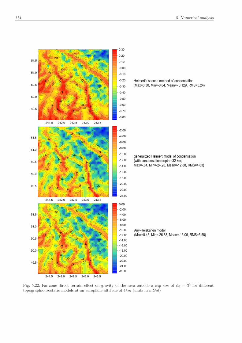
114 5. Numerical analysis
241.5 242.0 242.5 243.0 243.5
49.5
50.0
50.5
51.0
51.5
-0.80
-0.70
-0.60
-0.50
-0.40
-0.30
-0.20
-0.10
-0.00
0.10
0.20
0.30
Helmert's second method of condensation(Max=0.30, Min=-0.84, Mean=- 0.129, RMS=0.24)
Airy-Heiskanen model(Max=0.43, Min=-26.88, Mean=-13.05, RMS=5.58)
generalized Helmert model of condensation(with condensation depth =32 km;Max=-.64, Min=-24.26, Mean=-12.88, RMS=4.83)
241.5 242.0 242.5 243.0 243.5
49.5
50.0
50.5
51.0
51.5
-24.00
-22.00
-20.00
-18.00
-16.00
-14.00
-12.00
-10.00
-8.00
-6.00
-4.00
-2.00
241.5 242.0 242.5 243.0 243.5
49.5
50.0
50.5
51.0
51.5
-26.00
-24.00
-22.00
-20.00
-18.00
-16.00
-14.00
-12.00
-10.00
-8.00
-6.00
-4.00
-2.00
0.00
Fig. 5.22: Far-zone direct terrain effect on gravity of the area outside a cap size of ψ0 = 30 for differenttopographic-isostatic models at an aeroplane altitude of 4km (units in mGal)

5.3. Effects of topographic-isostatic masses at the surface of the Earth and at aeroplane altitudes 115
241.5 242.0 242.5 243.0 243.5
49.5
50.0
50.5
51.0
51.5
-24. 00
-22. 00
-20. 00
-18. 00
-16. 00
-14. 00
-12. 00
-10. 00
-8.0 0
-6.0 0
-4.0 0
-2.0 0
generalized Helmert model (Max=-0.631, Min=-24.285, Mean=-12.89, RSM=4.84)
di fferences between the effects at the sur face of the Earth and at an al ti tude of 6 km
241.5 242.0 242.5 243.0 243.5
49.5
50.0
50.5
51.0
51.5
-24.00
-22.00
-20.00
-18.00
-16.00
-14.00
-12.00
-10.00
-8.00
-6.00
-4.00
-2.00
241.5 242.0 242.5 243.0 243.5
49.5
50.0
50.5
51.0
51.5
-24.00
-22.00
-20.00
-18.00
-16.00
-14.00
-12.00
-10.00
-8.00
-6.00
-4.00
-2.00
height = 6 km
241.5 242.0 242.5 243.0 243.5
49.5
50.0
50.5
51.0
51.5
-0.010
0.000
0.010
0.020
0.030
0.040
0.050
241.5 242.0 242.5 243.0 243.5
49.5
50.0
50.5
51.0
51.5
-0.02
0.00
0.02
0.04
0.06
0.08
0.10
0.12
height =10 km di fferences between the effects at the sur face of the Ear th and at an a ltitude of 10 km
surface of the Earth
Fig. 5.23: Far-zone direct terrain effect on gravity of the area outside a cap size of ψ0 = 30 in case ofgeneralized Helmert method (D1 = 32 km) at different altitudes of the computation point (units in mGal)

116 5. Numerical analysis
241.5 242.0 242.5 243.0 243.5
49.5
50.0
50.5
51.0
51.5
-0.22
-0.18
-0.14
-0.10
-0.06
-0.02
0.02
0.06
0.10
Helmert's second method of condensation(Max=0.160, Min=-0.23, Mean=-0.09, RMS=0.09)
Airy-Heiskanen model(Max=10.85, M in=9.30, Mean=10.56, RMS=0.25)
general ized Helmert model of condensation(with condensation depth =32 km ;Max=13.23, Min=5.56, Mean=9.59, RMS=1.55)
241.5 242.0 242.5 243.0 243.5
49.5
50.0
50.5
51.0
51.5
6.00
7.00
8.00
9.00
10.00
11.00
12.00
13.00
241.5 242.0 242.5 243.0 243.5
49.5
50.0
50.5
51.0
51.5
9.40
9.60
9.80
10.00
10.20
10.40
10.60
10.80
Fig. 5.24: Far-zone primary indirect terrain effect on geoid heights of the area outside a cap size of ψ0 = 30
for different topographic-compensation models (units in meter)
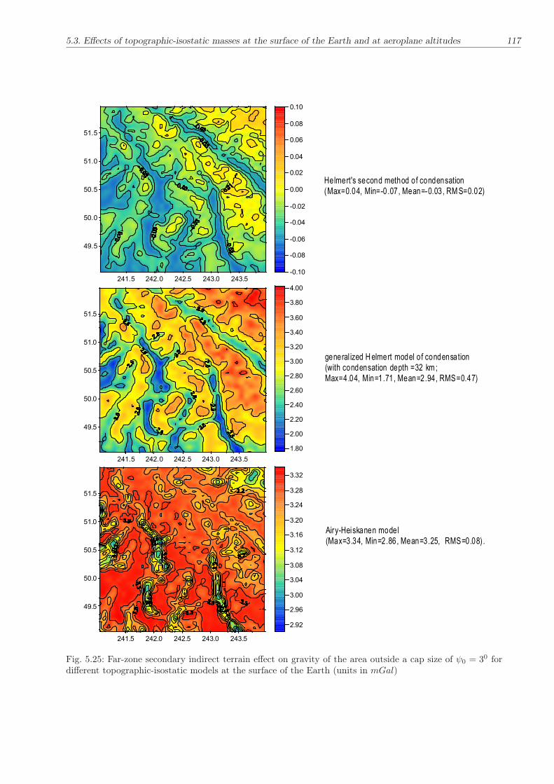
5.3. Effects of topographic-isostatic masses at the surface of the Earth and at aeroplane altitudes 117
241.5 242.0 242.5 243.0 243.5
49.5
50.0
50.5
51.0
51.5
-0.10
-0.08
-0.06
-0.04
-0.02
0.00
0.02
0.04
0.06
0.08
0.10
Helmert's second method of condensation(Max=0.04, Min=-0.07, Mean=-0.03, RMS=0.02)
Airy-Heiskanen model(Max=3.34, Min=2.86, Mean=3.25, RMS=0.08) .
general ized Helmert model of condensation(with condensation depth =32 km ;Max=4.04, Min=1.71, Mean=2.94, RMS=0.47)
241.5 242.0 242.5 243.0 243.5
49.5
50.0
50.5
51.0
51.5
1.80
2.00
2.20
2.40
2.60
2.80
3.00
3.20
3.40
3.60
3.80
4.00
241.5 242.0 242.5 243.0 243.5
49.5
50.0
50.5
51.0
51.5
2.92
2.96
3.00
3.04
3.08
3.12
3.16
3.20
3.24
3.28
3.32
Fig. 5.25: Far-zone secondary indirect terrain effect on gravity of the area outside a cap size of ψ0 = 30 fordifferent topographic-isostatic models at the surface of the Earth (units in mGal)

118 5. Numerical analysis
241.5 242.0 242.5 243.0 243.5
49.5
50.0
50.5
51.0
51.5
-0.80
-0.70
-0.60
-0.50
-0.40
-0.30
-0.20
-0.10
-0.00
0.10
0.20
0.30
Novàk et al. (2001)(Max=0.43, Min=-0.81, Mean=-0.09, RMS=0.23)
di fferences(Max=0.19, Min=-0.02, Mean=0.04, RMS=0.03)
the new formulae(Max=0.30, Min=-0.84, Mean=0.13, RMS=0.24)
241.5 242.0 242.5 243.0 243.5
49.5
50.0
50.5
51.0
51.5
-0.80
-0.70
-0.60
-0.50
-0.40
-0.30
-0.20
-0.10
-0.00
0.10
0.20
0.30
241.5 242.0 242.5 243.0 243.5
49.5
50.0
50.5
51.0
51.5
-0.01
0.01
0.03
0.05
0.07
0.09
0.11
0.13
0.15
0.17
Fig. 5.26: Far-zone direct terrain effects in case of Helmert’s second method of condensation at the surface ofthe Earth: (a) formulae in Novàk et al. (2001), (b) from Eq. (4.191), (c) differences between the two methods(units in mGal)

5.4. Effect of topographic-isostatic masses in satellite applications 119
for our test area – and a spherical harmonic expansion of the topography of up to degree Nmax = 360 takes48 sec on a PC (1, 8 GHz processor frequency). The computation costs are reduced further in case of largercap size radii, because in this case the upper degree of the spherical harmonic expansion can be reduced aswell.
5.3.2.4 Far-zone terrain effect on airborne gradiometry
The far-zone terrain effects at aeroplane altitude for the Himalaya region on z− component in a localcoordinates system of the gravity tensor, Vzz, are shown in Fig. 5.27. The cap size has been taken to be 30.Figure 5.27 shows that the effects of far-zone terrain effects are very small and in the size of approximatelyone percent of the total effect. This is caused by the fact that the second derivatives of the potential is inverseto the cubic distance between the computation and integration points which tapers off very quickly.
75 80 85 90 95 100
30
35
40
-0.50
-0.40
-0.30
-0.20
-0.10
-0.00
0.10
0.20
0.30
0.40
0.50
Fig. 5.27: Effects of the far-zone terrain on the tensor components Vzz of the area outside a cap size ofψ0 = 30 at an altitude of 10 km for the Airy-Heiskanen model for the Himalaya region (units in Eötvös)
5.4 Effect of topographic-isostatic masses in satellite applications
As we stated in section 4.1.2 and section 4.2 the effects of topographic-isostatic masses at satellite altitude canbe determined from the direct integration method or by a using spherical harmonic expansion. Therefore, thissection starts with the determination of the effects of topographic masses on Satellite Gravity Gradiometrybased on the two methods. The results have been compared and show the efficiency of the spherical harmonicapproach is demonstrated. Then the effects of the topographic-isostatic masses for different models at GOCEaltitude have been determined. Finally, the effects of the topographic-isostatic masses on POD (Precis orbitdetermination) and SST (Satellite-to-Satellite Tracking) observations are investigated.
5.4.1 Topographic-isostatic effects on gravity gradients
5.4.1.1 Computation formulae
To determine the effects of topographic-isostatic masses on the gravity gradients at GOCE altitude fromspherical harmonic expansions of the topography, the formulae derived by Tscherning (1976) are used for thepotential and its first and second derivations. The potential of the topographic-isostatic masses reads (ibid.):
V (r, ϕ, λ) =Gm
R
Nmax∑
n=0
(R
r
)n+1 n∑
m=0
(cnm cosmλ+ snm sinmλ)Pnm(sinϕ), (5.16)

120 5. Numerical analysis
its derivates with respect to ( r, ϑ, λ) yields (ibid.):
Vr(r, ϕ, λ) = −GmR2
Nmax∑
n=0
(n+ 1)
(R
r
)n+2 n∑
m=0
(cnm cosmλ+ snm sinmλ)Pnm(sinϕ), (5.17)
Vϕ(r, ϕ, λ) =Gm
R
Nmax∑
n=0
(R
r
)n+1 n∑
m=0
(cnm cosmλ+ snm sinmλ)∂Pnm(sinϕ)
∂ϕ, (5.18)
Vλ(r, ϕ, λ) =Gm
R
Nmax∑
n=0
(R
r
)n+1 n∑
m=0
m(−cnm sinmλ+ snm cosmλ)Pnm(sinϕ). (5.19)
The second derivatives can be determined by the formulae (ibid.)
Vrr(r, ϕ, λ) =Gm
R3
Nmax∑
n=0
(n+ 1)(n+ 2)
(R
r
)n+3 n∑
m=0
Pnm(sinϕ)(cnm cosmλ+ snm sinmλ), (5.20)
Vr,ϕ(r, ϕ, λ) = −GmR2
Nmax∑
n=0
(n+ 1)
(R
r
)n+2 n∑
m=0
(cnm cosmλ+ snm sinmλ)∂Pnm(sinϕ)
∂ϕ, (5.21)
Vr,λ(r, ϕ, λ) =Gm
R2
Nmax∑
n=0
(n+ 1)
(R
r
)n+2 n∑
m=0
m(cnm sinmλ− snm cosmλ)Pnm(sinϕ), (5.22)
Vλ,λ(r, ϕ, λ) = −GmR
Nmax∑
n=0
(R
r
)n+1 n∑
m=0
m2(cnm cosmλ+snm sinmλ)Pnm(sinϕ), (5.23)
Vϕ,ϕ(r, ϕ, λ) =Gm
R
Nmax∑
n=0
(R
r
)n+1 n∑
m=0
(cnm cosmλ+ snm sinmλ)∂2Pnm(sinϕ)
∂ϕ2, (5.24)
Vϕ,λ(r, ϕ, λ) =Gm
R
Nmax∑
n=0
(R
r
)n+1 n∑
m=0
m(−cnm sinmλ+ snm cosmλp)∂Pnm(sinϕ)
∂ϕ. (5.25)
In order to simplify the evaluation of the second derivatives of the gravitational potential, let us introducea tangential coordinate system frame at a point with spherical coordinates (r, ϕ, λ) as shown in Fig. 4.5 asfollows: the x-axis is directed to the north, the y- axis to the east, and the z-axis coincides with the radiusvector. Then the first and second derivatives of the gravitational potential with respect to x,y and z may berelated to the first and second derivatives with respect to r, ϕ, λ in the following equations:
Vx(r, ϕ, λ) =1
rVϕ, (5.26)
Vy(r, ϕ, λ) =1
r cosϕVλ, (5.27)
Vz(r, ϕ, λ) = Vr, (5.28)
Vxx(r, ϕ, λ) =1
rVr(r, ϕ, λ) +
1
r2Vϕϕ(r, ϕ, λ), (5.29)
Vxy(r, ϕ, λ) = Vyx(r, ϕ, λ) =1
r2 cosϕ(tanϕVλ(r, ϕ, λ) + Vϕλ(r, ϕ, λ)), (5.30)
Vxz(r, ϕ, λ) = Vzx(r, ϕ, λ) =1
r2(−Vϕ(r, ϕ, λ) + rVrϕ(r, ϕ, λ)), (5.31)
Vyy(r, ϕ, λ) =1
rVr(r, ϕ, λ) − tanϕ
r2Vϕ(r, ϕ, λ) +
1
r2 cos2 ϕVλλ(r, ϕ, λ), (5.32)

5.4. Effect of topographic-isostatic masses in satellite applications 121
Vyz(r, ϕ, λ) = Vzy(r, ϕ, λ) =1
r cosϕ(−1
rVλ(r, ϕ, λ) + Vrλ(r, ϕ, λ)), (5.33)
Vzz(r, ϕ, λ) = Vrr(r, ϕ, λ). (5.34)
Finally, the first and second derivatives of the potential can be calculated using the following formulae:
Vx(r, ϕ, λ) =GM
r2
Nmax∑
n=0
(R
r
)n n∑
m=0
(cosmλcnm + sinmλsnm)∂Pnm(sinϕ)
∂ϕ, (5.35)
Vy(r, ϕ, λ) =GM
r2 cosϕ
Nmax∑
n=0
(R
r
)n n∑
m=0
m(−cnm sinmλ+ snm cosmλ)Pnm(sinϕ), (5.36)
Vz(r, ϕ, λ) = −Gmr2
Nmax∑
n=0
(n+ 1)
(R
r
)n n∑
m=0
(cnm cosmλ+ snm sinmλ)Pnm(sinϕ), (5.37)
Vxx(r, ϕ, λ) =GM
r3
Nmax∑
n=0
(R
r
)n n∑
m=0
(cnm cosmλ+ snm sinmλ)
[
−(n+ 1)Pnm(sinϕ) +∂2Pnm(sinϕ)
∂ϕ2
]
,
(5.38)
Vxy(r, ϕ, λ) =GM
r3 cosϕ
Nmax∑
n=0
(R
r
)n n∑
m=0
m (−cnm sinmλ+ snm cosmλ)
[
tanϕPnm(sinϕ) +∂Pnm(sinϕ)
∂ϕ
]
,
(5.39)
Vxz(r, ϕ, λ) = −GMr3
Nmax∑
n=0
(R
r
)n
(n+ 2)
n∑
m=0
(cnm cosmλ+ snm sinmλ)∂Pnm(sinϕ)
∂ϕ, (5.40)
Vyy(r, ϕ, λ) =GM
r3
Nmax∑
n=0
(R
r
)n n∑
m=0
(cnm cosmλ+ snm sinmλ)
{[
−(n+ 1) − m2
cos2 ϕ
]
Pnm(sinϕ) − tanϕ∂Pnm(sinϕ)
∂ϕ
}
,
(5.41)
Vyz(r, ϕ, λ) =Gm
r3 cosϕ
Nmax∑
n=0
(n+ 2)
(R
r
)n n∑
m=0
m(cnm sinmλ− snm cosmλ)Pnm(sinϕ), (5.42)
Vzz(r, ϕ, λ) =GM
r3
Nmax∑
n=0
(n+ 1)(n+ 2)
(R
r
)n n∑
m=0
(cnm cosmλ+ snm sinmλ)Pnm(sinϕ). (5.43)
5.4.1.2 Integral formulae versus determination by spherical harmonic expansion
In order to get insight into the numerical differences between the numerical integration method and the sphe-rical harmonic expansion of the topography, the effects of the topographic masses on the second derivativesof the gravitational masses at GOCE altitude caused by the global topography have been determined byboth methods. In both cases the rock equivalent heights procedures with a resolution of 5 arc-minutes havebeen used. This fine grid size has been chosen to overcome the discretization errors in case of the numericalintegration method and to minimize the problem of the non-orthogonality of the discrete Legendre polynomi-als in case of the spherical harmonic expansion. The evaluation has been performed for the Asia region. Thedifferences between the numerical results of the discretized numerical integration and the spherical harmonicapproach are shown in Table 5.7. The table shows that the differences between the two methods are verysmall and can be neglected if we keep in mind the accuracy of the observation from the GOCE satellite(5 ∗ 10−3 Eötvös ). This means that it is better to use the spherical harmonic expansion for determining theeffects at satellite altitude as it sharply saves CPU time.

122 5. Numerical analysis
Table 5.7: Statistics of the differences between the numerical integration method and the spherical harmonicexpansion on the tensor component at an altitude of 250 km for Airy-Heiskanen model (units in Eötvös)
tensor components Max Min RMSxx 2.3E-5 -1.8E-4 2.8E-5yy 1.1E-4 -2.37E-5 1.5E-5zz 7.9E-5 -3.7E-6 1.7E-5
5.4.1.3 Computation of various topographic-isostatic models
The topographic-isostatic effects of the components of the gravitational tensor at a satellite altitude of 250km are already considerably damped (Fig. 5.28) compared to the features in an aircraft altitude of 10 km(Fig. 5.27) for the same region. Nevertheless, the structure of the topographic-isostatic effects at a satellitealtitude of 250 km shows still steep changes with a gradient of 0.70 Eötvös per 100 km in north-southdirection (Fig. 5.29) and of 0.50 m Eötvös per 100 km in east-west direction (Fig. 5.30).
75 80 85 90 95 100
30
35
40
-0.8
-0.6
-0.4
-0.2
-0.0
0.2
0.4
0.6
0.8
Fig. 5.28: Effects of the topographic-isostatic masses on the tensor component Vzz at an altitude of 250 kmfor the Airy-Heiskanen model for the Himalaya region; units in Eötvös)
If it is possible to remove this sort of roughness from the observations with a noise level of approximately5 ∗ 10−3 Eötvös expected for GOCE the downward continuation can be considerably simplified. The GOCEmission is designed to derive the static part of the gravity field with an extremely high precision. Therefore,it is very important to filter the observations by the topographic-isostatic gravity field effects to ease therequirements for the downward continuation. An additional regularization might be avoided in that case; butthis depends on the envisaged resolution of the gravity field model and on the error level of the observations.
Figs. 5.31 to 5.33 give an impression of the size of the effects of the topographic-isostatic masses for thexx, yy and zz-components of the gravitational tensor, respectively. The effects of the topographic-isostaticmasses for the Pratt-Hayford and the combined Airy-Pratt model are slightly larger than in case of the Airy-Heiskanen and Helmert’s first condensation model, while Helmert’s second condensation model producesonly tiny effects. The results indicate that the effects of topographic-isostatic masses and the gradient of thedifferent tensor components for different models are significant and it seems to be advantageous to take theminto account for the gravity field recovery of the GOCE observations. This question will be investigated in asimulation experiment.
Again, the coincidence of the generalized Helmert model of condensation with the other isostatic modelsdepends strongly on the condensation depths of Helmert’s model (Table 5.8 and Fig. 5.34). E.g, the ge-

5.4. Effect of topographic-isostatic masses in satellite applications 123
75 80 85 90 95 100
30
35
40
-0.5
-0.4
-0.3
-0.2
-0.1
-0.0
0.1
0.2
0.3
0.4
0.5
Fig. 5.29: Direction derivation of the tensor component Vzz in north-south direction at an altitude of 250km (effect of the topographic-isostatic masses on the tensor component Vzz for the Airy-Heiskanen modelfor the Himalaya region; units in Eötvös/degree)
75 80 85 90 95 100
30
35
40
-0.5
-0.4
-0.3
-0.2
-0.1
-0.0
0.1
0.2
0.3
0.4
0.5
Fig. 5.30: Direction derivation of the tensor component Vzz in west-east direction at an altitude of 250 km(effect of the topographic-isostatic masses on the tensor component Vzz for the Airy-Heiskanen model forthe Himalaya region; units in Eötvös/degree)

124 5. Numerical analysis
Vening Meinesz model(Max=0.65, Min=-0.77, Mean=-0.003, RMS=0.10)
A iry-Heiskanen model (Max=0.64, Min=-0.77, Mean=-0.003, RMS=0.09)
40 60 80 100 120 140 160-20
0
20
40
60
80
-0.40
-0.20
0.00
0.20
0.40
40 60 80 100 120 140 160-20
0
20
40
60
80
-0.40
-0.20
0.00
0.20
0.40
40 60 80 100 120 140 160-20
0
20
40
60
80
-0.40
-0.20
0.00
0.20
0.40
40 60 80 100 120 140 160-20
0
20
40
60
80
-0.40
-0.20
0.00
0.20
0.40
-20
0
20
40
60
80
40 60 80 100 120 140 160
-0.40
-0.20
0.00
0.20
0.40
40 60 80 100 120 140 160-20
0
20
40
60
80
-0.04
-0.02
0.00
0.02
0.04
Pratt-Hayford model (Max=0.65, Min=-0.76, Mean=-0.007, RMS=0.13)
combined Airy and Pratt model(Max=0.63, Min=-0.77, Mean=-0.007, RMS=0.12)
Helmert's first method(Max=0.37, Min=-0.42, Mean=-0.002, RMS=0.06)
Helmert's second method(Max=0.06, Min=-0.04, Mean=-0.000, RMS=0.01)
Fig. 5.31: Effects of the topographic-isostatic masses on the tensor component Vxx at an altitude of 250 kmfor different topographic-isostatic models (units in Eötvös)

5.4. Effect of topographic-isostatic masses in satellite applications 125
Vening Meinesz model(Max=0.38, Min=-0.44, Mean=0.002, RMS=0.07)
A iry-Heiskanen model (Max=0.38, Min=-0.45, Mean=0.002, RMS=0.07)
40 60 80 100 120 140 160-20
0
20
40
60
80
-0.40
-0.20
0.00
0.20
0.40
40 60 80 100 120 140 160-20
0
20
40
60
80
-0.40
-0.20
0.00
0.20
0.40
40 60 80 100 120 140 160-20
0
20
40
60
80
-0.40
-0.20
0.00
0.20
0.40
40 60 80 100 120 140 160-20
0
20
40
60
80
-0.40
-0.20
0.00
0.20
0.40
-20
0
20
40
60
80
40 60 80 100 120 140 160
-0.40
-0.20
0.00
0.20
0.40
40 60 80 100 120 140 160-20
0
20
40
60
80
-0.04
-0.02
0.00
0.02
0.04
Pratt-Hayford model (Max=0.49, Min=-0.69, Mean=0.005, RMS=0.12)
combined Airy and Pratt model(Max=0.48, Min=-0.65, Mean=-0.007, RMS=0.11)
Helmert's first method(Max=0.22, Min=-0.32, Mean=-0.000, RMS=0.06)
Helmert's second method(Max=0.03, Min=-0.03, Mean=-0.000, RMS=0.005)
Fig. 5.32: Effects of the topographic-isostatic masses on the tensor component Vyyat an altitude of 250 kmfor Helmert’s first method of condensation with different depths (units in Eötvös)

126 5. Numerical analysis
Vening Meinesz model(Max=0.97, Min=-0.65, Mean=0.003, RMS=0.14)
A iry-Heiskanen model (Max=0.98, Min=-0.66, Mean=0.003, RMS=0.14)
40 60 80 100 120 140 160
-20
0
20
40
60
80
-0.40
-0.20
0.00
0.20
0.40
40 60 80 100 120 140 160
-20
0
20
40
60
80
-0.40
-0.20
0.00
0.20
0.40
40 60 80 100 120 140 160
-20
0
20
40
60
80
-0.40
-0.20
0.00
0.20
0.40
40 60 80 100 120 140 160
-20
0
20
40
60
80
-0 .40
-0.20
0.00
0.20
0.40
-20
0
20
40
60
80
40 60 80 100 120 140 160
-0 .40
-0.20
0.00
0.20
0.40
40 60 80 100 120 140 160
-20
0
20
40
60
80
-0 .04
-0.02
0.00
0.02
0.04
Pratt-Hayford model (Max=0.99, Min=-0.76, Mean=0.007, RMS=0.21)
combined Airy and Pratt model(Max=0.98, Min=-0.75, Mean=0.008, RMS=0.20)
Helmert's first method (Max=0.55, Min=-0.37, Mean=0.002, RMS=0.10)
Helmert's second method(Max=0.07, Min=-0.05, Mean=-0.000, RMS=0.02)
Fig. 5.33: Effects of the topographic-isostatic masses on the tensor component Vzz at an altitude of 250 kmfor different topographic-isostatic models (units in Eötvös)
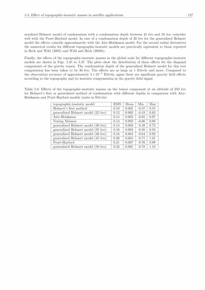
5.4. Effect of topographic-isostatic masses in satellite applications 127
neralized Helmert model of condensation with a condensation depth between 45 km and 50 km coincideswell with the Pratt-Hayford model. In case of a condensation depth of 30 km for the generalized Helmertmodel the effects coincide approximately with the Airy-Heiskanen model. For the second radial derivativesthe numerical results for different topographic-isostatic models are practically equivalent to those reportedin Heck and Wild (2005) and Wild and Heck (2004b).
Finally, the effects of the topographic-isostatic masses in the global scale for different topographic-isostaticmodels are shown in Figs. 5.35 to 5.37. The plots show the distribution of these effects for the diagonalcomponents of the gravity tensor. The condensation depth of the generalized Helmert model for this testcomputation has been taken to be 30 km. The effects are as large as 1 Eötvös and more. Compared tothe observation accuracy of approximately 5 ∗ 10−3 Eötvös, again these are significant gravity field effectsaccording to the topography and its isostatic compensation in the gravity field signal.
Table 5.8: Effects of the topographic-isostatic masses on the tensor component at an altitude of 250 kmfor Helmert’s first or generalized method of condensation with different depths in comparison with Airy-Heiskanen and Pratt-Hayford models (units in Eötvös)
topographic-isostatic model RMS Mean Min MaxHelmert’s first method 0.10 0.002 -0.37 0.55generalized Helmert model (25 km) 0.12 0.002 -0.43 0.63Airy-Heiskanen 0.14 0.003 -0.65 0.97Vening Meinesz 0.14 0.003 -0.66 0.98generalized Helmert model (30 km) 0.14 0.003 -0.49 0.73generalized Helmert model (35 km) 0.16 0.003 -0.56 0.83generalized Helmert model (40 km) 0.18 0.004 -0.64 0.92generalized Helmert model (45 km) 0.20 0.004 -0.71 1.01Pratt-Hayford 0.21 0.007 -0.76 0.99generalized Helmert model (50 km) 0.22 0.005 -0.78 1.10

128 5. Numerical analysis
40 60 80 100 120 140 160-20
0
20
40
60
80
-0.4
-0.2
0.0
0.2
0.4
40 60 80 100 120 140 160-20
0
20
40
60
80
-0.4
-0.2
0.0
0.2
0.4
40 60 80 100 120 140 160-20
0
20
40
60
80
-0.4
-0.2
0.0
0.2
0.4
40 60 80 100 120 140 160-20
0
20
40
60
80
-0.4
-0.2
0.0
0.2
0.4
-20
0
20
40
60
80
40 60 80 100 120 140 160
-0.4
-0.2
0.0
0.2
0.4
40 60 80 100 120 140 160-20
0
20
40
60
80
-0.4
-0.3
-0.2
-0.1
-0.0
0.1
0.2
0.3
0.4
condensation depth = 25 km condensation depth = 30 km
condensation depth = 35 km condensation depth = 40 km
condensation depth = 45 km condensation depth = 50 km
Fig. 5.34: Effects of the topographic-isostatic masses on the tensor component Vzz at an altitude of 250 kmfor generalized Helmert model of condensation with different depths (units in Eötvös)

5.4. Effect of topographic-isostatic masses in satellite applications 129
-150 -100 -50 0 50 100 150
-50
0
50
-0.40
-0.30
-0.20
-0.10
-0.00
0.10
0.20
0.30
0.40
-150 -100 -50 0 50 100 150
-50
0
50
-0.40
-0.30
-0.20
-0.10
-0.00
0.10
0.20
0.30
0.40
-150 -100 -50 0 50 100 150
-50
0
50
-0.40
-0.30
-0.20
-0.10
-0.00
0.10
0.20
0.30
0.40
-150 -100 -50 0 50 100 150
-50
0
50
-0.40
-0.30
-0.20
-0.10
-0.00
0.10
0.20
0.30
0.40
A iry-Heiskanen model(Max=0.59, Min=-0.80, Mean=0.00, RMS=0.07)
general ized Helmert model of condensation (Max=0.45, M in=-0.69, Mean=0.00, RMS=0.007)
Pratt-Hayford model(Max=0.65, M in=-0.96, Mean=0.00, RMS=0.12)
combined Airy and Pratt model(Max=0.62, M in=-0.90, Mean=0.00, RMS=0.11)
Fig. 5.35: Effects of the topographic-isostatic masses on the tensor component Vxx at an altitude of 250 kmfor different topographic-isostatic models (units in Eötvös)
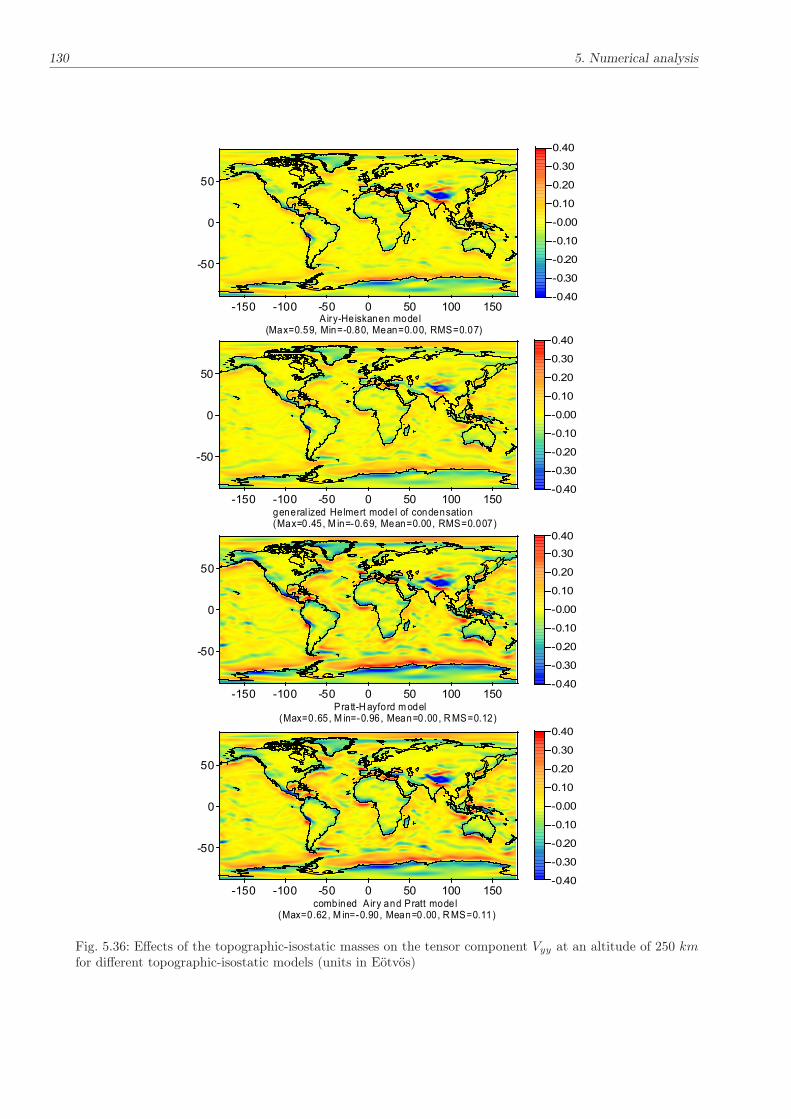
130 5. Numerical analysis
-150 -100 -50 0 50 100 150
-50
0
50
-0.40
-0.30
-0.20
-0.10
-0.00
0.10
0.20
0.30
0.40
-150 -100 -50 0 50 100 150
-50
0
50
-0.40
-0.30
-0.20
-0.10
-0.00
0.10
0.20
0.30
0.40
-150 -100 -50 0 50 100 150
-50
0
50
-0.40
-0.30
-0.20
-0.10
-0.00
0.10
0.20
0.30
0.40
-150 -100 -50 0 50 100 150
-50
0
50
-0.40
-0.30
-0.20
-0.10
-0.00
0.10
0.20
0.30
0.40
A iry-Heiskanen model(Max=0.59, Min=-0.80, Mean=0.00, RMS=0.07)
general ized Helmert model of condensation (Max=0.45, M in=-0.69, Mean=0.00, RMS=0.007)
Pratt-Hayford model(Max=0.65, M in=-0.96, Mean=0.00, RMS=0.12)
combined Airy and Pratt model(Max=0.62, M in=-0.90, Mean=0.00, RMS=0.11)
Fig. 5.36: Effects of the topographic-isostatic masses on the tensor component Vyy at an altitude of 250 kmfor different topographic-isostatic models (units in Eötvös)

5.4. Effect of topographic-isostatic masses in satellite applications 131
-150 -100 -50 0 50 100 150
-50
0
50
-0.40
-0.30
-0.20
-0.10
-0.00
0.10
0.20
0.30
0.40
-150 -100 -50 0 50 100 150
-50
0
50
-0.40
-0.30
-0.20
-0.10
-0.00
0.10
0.20
0.30
0.40
-150 -100 -50 0 50 100 150
-50
0
50
-0.40
-0.30
-0.20
-0.10
-0.00
0.10
0.20
0.30
0.40
-150 -100 -50 0 50 100 150
-50
0
50
-0.40
-0.30
-0.20
-0.10
-0.00
0.10
0.20
0.30
0.40
A iry-Heiskanen model(Max=1.23, Min=-0.66, Mean=0.004, RMS=0.13)
general ized Helmert model of condensation (Max=1.10, M in=-0.70, Mean=0.003, RMS=0.14)
Pratt-Hayford model(Max=1.44, M in=-0.99, Mean=0.004, RMS=0.21)
combined Airy and Pratt model(Max=1.34, M in=-0.93, Mean=0.003, RMS=0.19)
Fig. 5.37: Effects of the topographic-isostatic masses on the tensor component Vzz at an altitude of 250 kmfor different topographic-isostatic models (units in Eötvös)

132 5. Numerical analysis
5.4.2 Topographic-isostatic effects on SST observations
As sketched in chapter 2, the gravity field recovery from SST data is based on the analysis of short preciselydetermined kinematical orbits based mainly on GPS measurements in an altitude of ∼ 400 km.
5.4.2.1 Effects on the orbit
To get an impression of the size of the topographic-isostatic effects on the short arcs, a 30-minute-arc hasbeen determined dynamically twice, the first version based on EGM96 potential coefficients (Lemoine etal. 1998) complete up to degree Nmax = 360, the second version based on EGM96 minus the effects of thetopographic-isostatic masses. Then both orbits have been compared applying a least squares fit of both orbits.The differences in the coordinates represent the effect of the topographic-isostatic gravity field effects in theshort arcs. Figure 5.38 shows the effects of different topographic isostatic models. The Airy-Heiskanen modeland the Vening Meinesz model as well as the generalized Helmert model of condensation show significantdeviations up to two meters. The Pratt-Hayford model as well as the combined Pratt-Airy model show evenlarger deviations up to four meters while the gravity field effect of Helmert’s second model is very small,only a couple of centimeters.
5.4.2.2 Effects on the relative motion of two satellites
To investigate the gravity field effects of the topographic-isostatic models on the ranges and range-rates of atwin-satellite scenario like GRACE the relative orbits of a 30-minute-arc have been determined dynamicallytwice again: The first version has been based on EGM96 potential coefficients complete up to degree Nmax =360, the second one based on EGM96 coefficients minus the effects of the topographic-isostatic models. Thenboth relative orbits have been compared applying a least squares fit of both relative orbits.
The differences in the ranges and range-rates represent the effect of the topographic-isostatic gravity fieldeffects in the short relative arcs. Figure 5.39 shows the effects of the topographic-isostatic models in theranges and Fig. 5.40 in the range-rates. Again the Airy-Heiskanen model and the Vening Meinesz model aswell as the generalized Helmert model of condensation show significant deviations up to a couple of decimeterswhile the gravity field effect of Helmert’s second model again is very small. Also, the Pratt-Hayford modeland the combined Airy-Pratt model show significant deviations larger than the other models.
The situation is similar in case of the topographic-isostatic effects in the range-rates between the GRACEsatellites. Again the Airy-Heiskanen model and the Vening Meinesz model as well as the Helmert’s first orgeneralized condensation method show significant deviations up to ±200 to 300µm/s while the gravity fieldeffect of Helmert’s second model is very small. In addition, the effect of the Pratt-Hayford model and thecombined Airy-Pratt model show significant deviations larger than those of the other models. Compared tothe observation accuracy of approximately 0.2µm/s these are significant effects in the gravity field signal.

5.4. Effect of topographic-isostatic masses in satellite applications 133
51740 51740.005 51740.01 51740.015 51740.02
MJD (days)
-4
-3
-2
-1
0
1
2
Deviation (m)
Airy-Heiskanen model
x-coordinate
y-coordinate
z-coordinate
51740 51740.005 51740.01 51740.015 51740.02
MJD (days)
-4
-3
-2
-1
0
1
2
Deviation (m)
Vening Meinesz model
x-coordinate
y-coordinate
z-coordinate
51740 51740.005 51740.01 51740.015 51740.02
MJD (days)
-0.12
-0.08
-0.04
0
0.04
0.08
Deviation (m)
Helmert's second method of condensationx-coordinate
y-coordinate
z-coordinate
51740 51740.005 51740.01 51740.015 51740.02
MJD (days)
-4
-2
0
2
Deviation (m)
Helmert's first method of condensation(D=30 km)
x-coordinate
y-coordinate
z-coordinate
51740 51740.005 51740.01 51740.015 51740.02
MJD(days)
-4
-2
0
2
Deviation(m
)
Combined Airy and Pratt model
x- coordinate
y-coordinate
z-coordinate
51740 51740.005 51740.01 51740.015 51740.02
MJD (days)
-6
-4
-2
0
2
Deviation (m)
Pratt-Hayford model
x-coordinate
y-coordinate
z-coordinate
Fig. 5.38: Orbit deviations for different topographic isostatic models (altitude: ∼400 km)
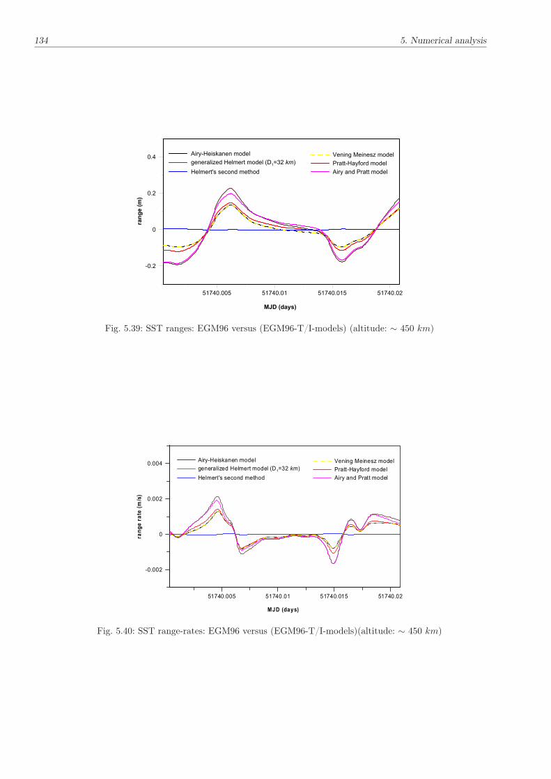
134 5. Numerical analysis
51740.005 51740.01 51740.015 51740.02
MJD (days)
-0.2
0
0.2
0.4
range (m)
Vening Meinesz model
Pratt-Hayford model
Airy and Pratt model
Airy-Heiskanen model
generalized Helmert model (D1=32 km)
Helmert's second method
Fig. 5.39: SST ranges: EGM96 versus (EGM96-T/I-models) (altitude: ∼ 450 km)
51740.005 51740.01 51740.015 51740.02
MJD (days)
-0.002
0
0.002
0.004
range rate (m/s)
Vening Meinesz model
Pratt-Hayford model
Airy and Pratt model
Airy-Heiskanen model
generalized Helmert model (D1=32 km)
Helmert's second method
Fig. 5.40: SST range-rates: EGM96 versus (EGM96-T/I-models)(altitude: ∼ 450 km)
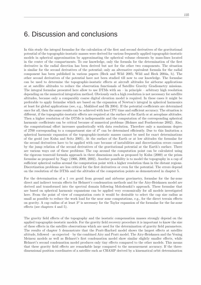
135
6. Discussion and conclusions
In this study the integral formulae for the calculation of the first and second derivatives of the gravitationalpotential of the topographic-isostatic masses were derived for various frequently applied topographic-isostaticmodels in spherical approximation by approximating the spherical volume elements by mass-lines locatedin the center of the compartments. To our knowledge, only the formula for the determination of the firstderivative in the radial direction has been derived but not for the other two components. The situationis similar for the second derivatives of the potential; only an alternative equivalent formula for the radialcomponent has been published in various papers (Heck and Wild 2005; Wild and Heck 2004a, b). Theother second derivatives of the potential have not been studied till now to our knowledge. The formulaecan be used to determine the topographic-isostatic effects at aircraft altitudes for airborne applicationsor at satellite altitudes to reduce the observation functionals of Satellite Gravity Gradiometry missions.The integral formulae presented here allow to use DTMs with an – in principle – arbitrary high resolutiondepending on the numerical integration method. Obviously such a high resolution is not necessary for satellitealtitudes, because only a comparably coarse digital elevation model is required. In these cases it might bepreferable to apply formulae which are based on the expansion of Newton’s integral in spherical harmonicsat least for global applications (see, e.g., Makhloof and Ilk 2004). If the potential coefficients are determinedonce for all, then the same results can be achieved with less CPU time and sufficient accuracy. The situation isdifferent, if the topographic-isostatic effects are required at the surface of the Earth or at aeroplane altitudes.Then a higher resolution of the DTMs is indispensable and the computation of the corresponding sphericalharmonic coefficients can be critical because of numerical problems (Holmes and Featherstone 2002). Also,the computational effort increases quadratically with data resolution. Therefore only a maximum degreeof 2700 corresponding to a compartment size of 4′′ can be determined efficiently. Due to this limitation aspherical harmonic expansion of the topographic-isostatic masses cannot be used for exact determinationsof the geoid (see Kuhn and Seitz 2005). At the surface of the Earth or at low altitudes the formulae forthe second derivatives have to be applied with care because of instabilities and discretization errors causedby the jump relation of the second derivatives of the gravitational potential at the Earth’s surface. Thereare various ways out of these problems: The cap around the computation point can be calculated usingthe rigorous tesseroid formula approach in three dimensions such as proposed by Kuhn (2000) or the prismformulae as proposed by Nagy (1966, 2000, 2002). Another possibility is to model the topography in a cap ofsufficient spherical radius around the computation point with a higher resolution than in the distant regions.Discretization problems are less critical for the first derivatives or even for the potential. The errors dependon the resolution of the DTMs and the altitudes of the computation points as demonstrated in chapter 5.
For the determination of a 1 cm geoid from ground and airborne gravimetry, formulae for the far-zonedirect and indirect terrain effects for Helmert’s condensation methods and for the Airy-Heiskanen model arederived and transformed into the spectral domain following Molodenskii’s approach. These formulae thatare based on spherical harmonic expansions can be applied very economically for all models investigatedhere. From the point of view of computation costs it would be desirable to select the cap size radius assmall as possible to reduce the work load for the near zone computations, e.g., for the direct terrain effectson gravity. A cap radius of at least 3o is necessary for the Taylor expansion of the formulae for the far-zoneeffects (see chapters 4 and 5).
The gravity field effects of the topography and the isostatic compensation masses strongly depend on theapplied topographic-isostatic models. For the gravity field recovery procedure it is important to know the sizeof these effects in the satellite observations which are used for the determination of gravity field parameters.The results of chapter 5 demonstrate that the Pratt-Hayford model shows the largest effects at satellitealtitude, followed – as expected – by the combined Airy and Pratt model. The Airy-Heiskanen and the VeningMeinesz models as well as Helmert’s first condensation model show similar slightly smaller effects, whileHelmert’s second condensation model produces only tiny effects compared to the other models. This meansthat these gravity field effects are remarkable large compared to the measurement accuracy. If the three-dimensional position coordinates of a satellite such as CHAMP derived by a kinematical orbit determination

136 6. Discussion and conclusions
procedure are used within the so-called Precise Orbit Determination (POD) gravity field recovery approachthen the coordinates must be known with an accuracy of one to two centimeters. It becomes obvious thatan effect in the orbit of up to a couple of meters (as shown in chapter 5) corresponding to a signal-to-noiseratio of approximately 1000 requires a careful computation of the topographic-isostatic effects. The situationis similar if low-low SST data of a GRACE-type twin satellite mission are used for the gravity field recovery.Again the ratio of the topographic-isostatic effect to the measurement noise is approximately 1000 for theseobservables. This holds approximately for all models except for Helmert’s second condensation method. Thetopographic-isostatic effects might be also important for the gravity field mission GOCE where the gravitygradients are measured with high precsion, especially the diagonal elements. The size of the diagonal elementsof the gravity gradients is largest for the radial component Vzz and approximately half of these values for thelocal horizontal components Vxx and Vyy. Also in this case the signal-to-noise ratio is approximately 1000 ifwe take into account the measurement accuracy of the Satellite Gravity Gradiometry mission GOCE in thesize of 0.003 Eötvös. Therefore, also in this case a remove-restore procedure can significantly stabilize thedownward continuation procedure and can help to improve the final results.
The far-zone direct terrain effects are rather high for Helmert’s first or generalized condensation methodas well as for the Airy-Heiskanen model and very small in case of Helmert’s second condensation method.It is interesting to note that the altitude of the computation point has a minor influence on the size ofthe far-zone effects for all topographic-compensation models. The far-zone effects decrease slightly withincreasing altitude and are more or less identical in case of cap radii of 10o and larger. Therefore, the resultshold for ground gravity measurements and for airborne gravimetry. The far-zone effects increase with thecondensation depth selected for the generalized Helmert model (and are very small for the second Helmertmethod). A corresponding behaviour show the numerical tests for the far-zone primary and secondary indirectterrain effects. An important question is the selection of the cap radius for the determination of far-zonetopographic-compensation effects. For Helmert’s second method of condensation the far-zone terrain effectsin case of a cap radius of 3o and larger have a minor influence on airborne gravity measurements in relationto a measurement accuracy of 1 to 2 mGal and can be omitted completely. The situation is different in caseof ground gravity measurements with a much higher measurement accuracy of 0.02 mGal. In this case thefar-zone effects have to be considered in case, e.g. of a cap radius of 3o. The maximum harmonic degree of50 should be sufficient for the determination of the far-zone effects in this case. The situation is differentin case of Helmert’s generalized condensation models (including Helmert’s first model) and in case of theAiry-Heiskanen model. Even in case of the minor accuracy of airborne gravimetry the far-zone effects haveto be considered for cap radii of 3o and also larger ones. The maximum degree of the spherical harmonicexpansion can be restricted to 50 in case of airborne gravimetry and up to degree 200 and higher for groundgravity measurements, depending on the accuracy demands. If we keep in mind that the accuracy of theairborne gravimetry is 1-2 mgal and the band limted geoid is determined, then it is better to use spacelocalizing space function than the integral formulae for determinig the topographic-compensating masseseffects.
Now the question arises which model should preferably be used for the filtering of satellite born observationssuch as low-low SST data, airbore gravimetry, three-dimensional position coordinates or measured gravitygradients as preparation for the subsequent downward continuation procedure? While Helmert’s secondcondensation method might be useful for geoid computations, its usefulness for the processing of satellitein-situ observations cannot be answered in such a simple generally valid way. Indeed the task of filteringtopographic-isostatic effects in the satellite observations is helpful only if these quantities show a significantsize in the observations. Obviously, this fact depends on the validity of the topographic-isostatic hypothesisin specific geographic regions. This can be decided only after a careful analysis of the specific gravity fieldfeatures within the various geographical regions of the Earth to find out which model describes the realityin these regions in the best possible way. It is well-known that the Earth is isostatically compensated byan amount of approximately 90%, but it is difficult to decide which model fits best. Although seismicmeasurement results indicate the validity of an Airy-Heiskanen type of topographic-isostatic compensation,in some parts of the Earth the isostatic compensation seems to follow the Pratt-Hayford model (Heiskanenand Moritz 1967). If the specific topographic-isostatic model holds more or less uniformly for a larger regionthen this model can be used to filter the satellite observations before the application of the regional gravityfield recovery procedure. The situation is more complicated in case of regionally varying deviations of the
137
reality from a specific model; further investigations are necessary to consider this case. The numerical resultsindicate that the effects of topographic and isostatic masses for Helmert’s first method of condensation witha condensation depth of 30 km coincides approximately with the effects of the Airy-Heiskanen model. Thechange of the condensation level by using a sort of generalized Helmert model (Heck 2003) could be usedto fit the topographic-isostatic model to the reality. An interesting side effect would be the reduction of thecomputation costs due to the efficiency of this model.
Because of the varying effects of the topographic-isostatic models depending on the type of observables suchas gravity vectors or tensor components the frequently expressed argument that a high resolution gravity fieldmodel might be sufficient to reduce observations at aeroplane or satellite altitude is not valid. Therefore,additional investigations are necessary to demonstrate the benefit of a remove-restore procedure takinginto account individually selected topographic-isostatic models for the processing of airborne measurementsand SGG observables. Therefore, an integration of this processing steps into the global but especially theregional gravity field recovery procedure as developed at the Institute of Theoretical Geodesy, University ofBonn, and various other aspects mentioned here have to be investigated. In addition, further investigationsare necessary to demonstrate the benefit of a remove-restore procedure taking into account topographic-compensation effects for the processing of POD and low-low SST observables. Also, further investigationsare necessary to take the cubic terms of the Taylor expansion into account in the case of the Airy-Heiskanenmodel. Also, further investigation can be performed to apply the Molodenskii’s approach for determingthe far-zone effects for other topographic-isostatic models such as the Pratt-Hayford model. Finally, thegeophysical models in coincidence with modern models of plate tectonics must be investigated with respectto its topographic-isostatic effects.
Acknowledgement
This research was carried out in the framework of the exchange grant by the Egyptian government in theInstitute of Theoretical Geodesy, University of Bonn. I have received a great support during my research,therefore I would like to address my special thanks to the following persons: I would like to express my deepand sincere appreciation to my research advisor Prof. Dr. Karl Heinz Ilk for offering me the opportunity tocarry out my research in his institute, for his guidance, helpful advice and supervision. I am indebted to hisconstant encouragement and fruitful and interesting discussions throughout this work. Most importantly,his ever willingness and dedication to solve my personal and numerical problems worth more mention.He has critically read this thesis and his valuable comments and suggestions are gratefully appreciated. Iwould like to express my deep thanks to Prof. Dr. Bertold Witte for his evaluation of my thesis. I wish toexpress my deep gratitude to Prof. Dr. Hussein Abd-Elmotaal, Faculty of Engineering, Minia University,for his encouragement. I am deeply indepted to the secretaries of the Institute of Theoretical Geodesy, Mrs.Schleifenbaum and Mrs. Losch, for their generous continous help and to all members of the Institute for theirhelp during my stay in Bonn. To my friend Anno Löcher (Institute of Theoretical Geodesy, Bonn University)for his help during programming, his help during writing in Latex and for reading the thesis. I wouldlike to thank the Egyptian Ministry of Higher Education, the Faculty of Engineering, Minia University,Egypt for providing me with a Ph.D. scholarship. To my colleagues of the Civil Engineering Department,Faculty of Engineering, Minia University, Egypt, for their continuous encouragement. My special thanksand appreciations are also due to my wife for her continuous encouragements and for providing me with anexcellent environment and atmosphere for doing my research work. To my children who are in Egypt andwho are here with me in Bonn. Lastly, very special thanks to my father, my mother, my sisters for theirheartily feelings and continuous prayers. To all of you, thank you very much.
Atef Abdel-Hakeem MakhloofBonn, Germany

138
References
Abd-Elmotaal H (1991): Gravity anomalies based on the Vening Meinesz isostatic model and their statisticalbehavior. Mitteilung der Geodätischen Institute der Technischen Universität Graz, Folge 72
Abd-Elmotaal H (1995a): Theoretical background of the Vening Meinesz isostatic model. In: H. Sünkel andI. Marson (eds.): Gravity and Geoid. Joint Symposium of the International Gravity Commission and theInternational Geoid Commission, Symposium No. 113, pp. 268-277. Springer Verlag, Berlin, Heidelberg,New York
Abd-Elmotaal H (1995b): Attraction of the topographic masses, Bulletin Géodésique, 69(4): 304-307
Abd-Elmotaal H (1999): Comparison among different geoid solutions for the Egyptian south-western desertusing FFT technique. Bolletino di Geofisica Teorica ed Applicata 40(3-4): 563-569
Anderson EG (1976): The effect of topography on solutions of Stokes’ problem. Unisurv Report S14, Uni-versity of New South Wales, Kensington, Australia
Banks RJ, Parker RL, Huestis SP (1977): Isostatic compensation on a continental scale: local versus regionalmechanisms. The geophysical journal of the Royal Astronomical Society 51: 431-452
Blakely RJ (1995): Potential theory in gravity and magnetic applications. Cambridge University Press,Cambridge, UK
Bracewell R (1978): The Fourier transform and its applications. 2nd edn., McGraw-Hill, New York
Bruns H (1878): Die Figur der Erde. Publication des Königl.-Preuss. Geodätischen Institutes, Berlin
Claessens S (2003): A synthetic Earth model; analysis, implementation; validation and application. DelftUniversity Press, Delft, The Netherlands
Colombo OL (1981): Numerical methods for harmonic analysis on the sphere. Reports of the Department ofGeodetic Science and Surveying No. 310, Ohio State University, Columbus, Ohio
Courant R, Hilbert D (1953): Methods of the mathematical physics. Volume 1, Interscience Publishers, NewYork, London
Dutton CE (1889): On some of the greater problems of physical geology. Bulletin of the Philosophical Societyof Washington, 11: 51-64
Eicker A, Mayer-Gürr T, Ilk KH (2004): Global gravity field solutions based on a simulation scenario ofGRACE SST data and regional refinements by GOCE SGG observations. In: Jekeli C, Bastos L, Fern-andes J (eds.): Gravity, Geoid and Space Missions. International Association of Geodesy Symposia, Vol.129, Springer, Berlin, Heidelberg, New York, pp. 66-71
Engels J, Grafarend E (1993): The gravitational field of topographic-isostatic masses and the hypothesis ofmass condensation. Surveys in Geophysics 140: 495-524
European Space Agency (1999): Gravity Field and Steady-State Ocean Circulation Explorer Mission (GO-CE), Report for mission selection, in: The four canditate Earth explorer core missions, SP-1233, Nord-wijk, The Netherlands
Featherstone WE (1992): A GPS controlled gravimetric determination of the geoid of the British Isles. D.Phil.thesis, University of Oxford, England
Featherstone WE, Kirby JF, Kearsley AHW, Gilliland JR, Johnston GM, Steed J, Forsberg R, Sideris MG(2001): The AUSGeoid98 geoid model of Australia: data treatment, computations and comparisons withGPS-levelling data. Journal of Geodesy 75(5-6): 313-330

References 139
Forsberg R (1984): A study of terrain reduction, density anomalies and geophysical inversion method ingravity field modelling. Reports of the Department of Geodetic Science and Surveying No. 335, OhioState University, Columbus, Ohio
Forsberg R (1985): Gravity field terrain effect computation by FFT. Bulletin Géodésique 59: 342-360
Forsberg R, Sideris MG (1993): Geoid determination by multi-band spherical FFT approach. ManuscriptaGeodaetica 18: 82-90
Forsberg R, Tscherning CC (1997): Topographic effects in gravity field modelling for BVP. In: Sansó F,Rummel R (eds.) Geodetic boundary value problems in view of the one centimetre geoid. Lecture Notesin Earth Sciences, Vol. 65. Springer, Berlin, Heidelberg, New York, pp 241-272
Freeden W, Windheuser U (1996): Spherical wavelet transform and its discretization. Advances in Compu-tational Mathematics 5: 51-94
Freeden W, Gervens T, Schreiner M (1998): Constructive approximation on the sphere. Oxford UniversityPress, Oxford, England
Gauss CF (1839): Allgemeine Theorie des Erdmagnetismus. In: Gauss CF and Weber W: Resultate aus denBeobachtungen des Magnetischen Vereins im Jahre 1838., Göttingen und Leipzig
Gradshteyn IS, Ryzhik IM (1980): Tables of Integrals, Series, and Products. Academic Press, New York
Grüninger W (1990): Zur Topographisch-Isostatischen Reduktion der Schwere. Ph.D. thesis, Technical Uni-versity Karlsruhe
Haagmans R (2000): A synthetic Earth for use in geodesy. Journal of Geodesy 74(7-8): 503-511
Harrison JG, Dickinson M (1989): Fourier transforms method in local gravity field modelling. Bulletin Géo-désique 63: 49-166
Heck B (1992): A revision of Helmert’s second method of condensation in geoid and quasi-geoid determination.In: Montag H, Reigber C (eds.): Geodesy and Physics of the Earth. International Association of GeodesySymposia, Vol. 112, Springer, Berlin, Heidelberg, New York, pp. 246-251
Heck B (2003): On Helmert’s methods of condensation, Journal of Geodesy 77(3-4): 155-170
Heck B and Wild F (2005): Topographic-isostatic reductions in Satellite Gravity Gradiometry based on ageneralized condensation model. In: Sansó F (ed.): A Window on the Future of Geodesy, InternationalAssociation of Geodesy Symposia, Vol. 128, Springer, Berlin, Heidelberg, New York, pp. 294-299
Heck B and Seitz F (2006): A comparison of the tesseroid, prism and point-mass approaches for massreductions in gravity field modelling. Journal of Geodesy 81(2):121-136
Heiskanen WA, Vening Meinesz FA (1958): The Earth and its gravity field. McGraw-Hill, New York
Heiskanen WA, Moritz H (1967): Physical Geodesy. W.H. Freeman and Company, San Francisco and London
Helmert FR (1884): Die mathematischen und physikalischen Theorien der höheren Geodäsie. Band II, Teub-ner, Leipzig. Reprint: Minerva, Frankfurt a. M. 1962
Hertz H (1884): Über das Gleichgewicht schwimmender elastischer Platten, Annalen der Physik und Chemie22: 449-455
Holmes SA and Featherstone WE (2002): A unified approach to the Clenshaw summation and the recursivecomputation of very high degree and order normalized associated Legendre functions. Journal of Geodesy76(5): 279-299
Hotine M (1969): Mathematical Geodesy. U. S. Government Printing Office, Washington, D.C.

140 References
Huang J, Vaníček P, Pagiatakis SD, Brink W (2001): Effect of topographical density on geoid in the CanadianRocky Mountains. Journal of Geodesy 74(11-12): 805-815
Jeffreys H (1976): The Earth: its origin, history and physical constitution, 6th edn., Cambridge UniversityPress, Cambridge, UK
Kertz W (1969): Einführung in die Geophysik. Band I: Erdkörper. Bibliographisches Institut, Mannheim
Kiamehr R and Sjöberg LE (2005): Effect of the SRTM global DEM on the determination of a high-resolutiongeoid model: a case study in Iran. Journal of Geodesy 79(9): 540-551
Kirby JF, Featherstone WE (1999): Terrain correcting the Australian gravity observations using the nationaldigital elevation model and the Fast Fourier Transform, Australian Journal of Earth Science 46: 555-562
Klees R (1992): Lösung des fixen geodätischen Randwertproblems mit Hilfe der Randelementemethode.Deutsche Geodätische Kommission, Reihe C, Nr. 382, München
Klose U, Ilk KH (1993): A solution to the singularity problem occurring in the terrain correction formula.Manuscripta Geodaetica 18: 263-279
Koch KR (1965): Die topographische Schwere- und Lotabweichungsreduktion für Aufpunkte in geneigtemGelände. Allgemeine Vermessungsnachrichten 11: 438-441
Koch KR, Kusche J (2003): Regularization of geopotential determination from satellite data by variancecomponents estimation, Journal of Geodesy 76(5): 259-268
Krylov VI (1962): Approximate calculation of integrals. MacMillan, New York
Kuhn M (2000a): Geoidbestimmung unter Verwendung verschiedener Dichtehypothesen. Deutsche Geodäti-sche Kommission, Reihe C, Nr. 520, München
Kuhn M (2000b): Density modelling for geoid determination. In: Sideris MG (ed.): Gravity, Geoid and Geo-dynamics 2000. International Association of Geodesy Symposia, Vol. 123, Springer, Berlin, Heidelberg,New York, pp. 271-276
Kuhn M (2002): On the indirect effect of Helmert’s condensation methods. International Geoid Service 13:50-52
Kuhn M (2003): Geoid determination with density hypotheses from isostatic models and geological informa-tion. Journal of Geodesy 77(1-2): 50-65
Kuhn M, Seitz K (2005): Comparison of Newton’s integral in the space and frequency domains. In: Sansó F(ed.): A Window on the Future of Geodesy, International Association of Geodesy Symposia, Vol. 128,Springer, Berlin, Heidelberg, New York, pp. 386-391
Lambeck K (1988): Geophysical geodesy, the slow deformations of the Earth. Clarendon Press, Oxford, UK
Lanczos C (1956): Applied analysis. Prentice Hall, Englewood Cliffs, N.J.
Landau LD, Lifshitz EM (1959): Theory of elasticity. 3rd edn., Pergamon Press, Oxford, UK
Lehmann R (1994): Zur Bestimmung des Erdschwerefeldes unter Verwendung des Maximum-Entropie-Prinzipes. Deutsche Geodätische Kommission, Reihe C, Nr. 425, München
Lemoine FG, Kenyon SC, Factor JK, Trimmer RG, Pavlis NK, Chinn DS, Cox CM, Klosko SM, Luthcke SB,Torrence MH, Wang YM, Williamson RG, Pavlis EC, Rapp RH, Olson TR (1998): The developmentof the joint NASA GSFC and the National Imagery and Mapping Agency (NIMA) geopotential modelEGM96. NASA/TP-1998-206861, Goddard Space Flight Center, Greenbelt, Maryland
Li YC, Sideris MG (1994): Improved gravimetric terrain corrections. Geophysical Journal International 119:740-752

References 141
MacMillan WD (1930): Theoretical Mechanics, vol 2: the Theory of the potential. McGraw-Hill, New York(reprinted by Dover Publications, New York 1958)
Mader K (1951): Das Newtonsche Raumpotential prismatischer Körper und seine Ableitung bis zur drittenOrdnung. Sonderheft 11 der Österreichischen Zeitschrift für Vermessungswesen, Wien
Makhloof AA, Ilk KH (2004): The use of topographic-isostatic gravity field information in Satellite-to-Satellite tracking and Satellite Gravity Gradiometry. Poster presented at the IAG International Sym-posium Gravity, Geoid and Space Missions, Porto
Makhloof AA, Ilk KH (2006): Effects of topographic-isostatic masses on gravitational functionals at thesurface of the Earth, at airborne and satellite altitudes, submitted to Journal of Geodesy
Márkus G (1978): Theorie und Berechnung rotationssymmetrischer Bauwerke. 3. Auflage, Werner-Verlag,Düsseldorf
Martinec Z (1993): Effect of lateral density variation of topographical masses in view of improving geoidmodel accuracy over Canada. Final Report under DSS Contract No. 23244-2-4356/01-SS, GeodeticSurvey of Canada, Ottawa
Martinec Z (1998): Boundary-value problems for gravimetric determination of a precise geoid. Lecture Notesin Earth Sciences, Vol. 73, Springer, Berlin, Heidelberg, New York
Martinec Z, Vaníček P (1994a): The indirect effect of Stokes-Helmert’s technique for a spherical approxima-tion of the geoid. Manuscripta Geodetica 18: 213-219
Martinec Z, Vaníček P (1994b): Direct topographical effect of Helmert’s condensation for a spherical geoid.Manuscripta Geodaetica 19: 257-268
Martinec Z, Matyska C, Grafarend EW, Vaníček P (1993): On Helmert’s second condensation method.Manuscripta Geodetica 18: 417-421
Martinec Z, Vaníček P, Mainville A, Véronneau M (1996): Evaluation of the topographic effects in precisegeoid computation from densely sampled heights. Journal of Geodesy 70(11): 746-754
Matyska C (1994): Topographic masses and mass heterogeneities in the upper mantle. In: Schutz BE, An-derson A, Froidevaux C, Parke M (eds.): Gravimetry and Space Techniques Applied to Geodynamicsand Ocean Dynamics, Geophysical Monograph 82, pp. 125-132
Mayer-Gürr T (2006): Gravitationsfeldbestimmung aus der Analyse kurzer Bahnbögen am Beispiel der Sa-tellitenmissionen CHAMP und GRACE. Ph.D. thesis, University Bonn
Mayer-Gürr T, Ilk KH, Eicker A, Feuchtinger M (2005): ITG-CHAMP01: A CHAMP gravity field modelfrom short kinematical arcs of a one-year observation period, Journal of Geodesy 78: 462-480
Mayer-Gürr T, Eicker A, Ilk KH (2006): Gravity field recovery from GRACE-SST data of short arcs. In:Flury J, Rummel R, Reigber C, Rothacher M, Boedecker G, Schreiber U (eds.): Observation of theEarth System from Space. Springer, Berlin, Heidelberg, New York, pp. 131-148
Molodenskii MS, Fremeev VF, Yurkina MI (1962): Methods for the study of the external gravitational fieldand figure of the Earth. Office of Technical Services, Department of Commerce, Washington, D.C.
Moritz H (1965): The boundary value problem of physical geodesy. Publication of the Isostatic Institute ofthe IAG, No. 50, Helsinki
Moritz H (1968): Linear solution of the geodetic boundary-value problem. Deutsche Geodätische Kommission,Reihe A, Heft 58, München
Moritz H (1980): Advanced physical geodesy. Herbert Wichmann Verlag, Karlsruhe
142 References
Nahavandchi H, Sjöberg LE (1998): Terrain corrections to power H3 in gravimetric geoid determination,Journal of Geodesy 72(3): 124-135
Nagy D (1966): The gravitational attraction of a right rectangular prism. Geophysics 31: 362-371
Nagy D, Papp G, Benedek J (2000): The gravitational potential and its derivatives for the prism. Journal ofGeodesy 74(7-8): 552-560
Nagy D, Papp G, Benedek J (2002): Correction to The gravitational potential and its derivatives for theprism“, Journal of Geodesy 76(8): 475
Neumann F (1838): Über eine neue Eigenschaft der Laplaceschen Y n und ihre Anwendung zur analytischenDarstellung derjenigen Phänomene, welche Functionen der geographischen Länge und Breite sind, Schu-machers Astronomische Nachrichten, 15: 313-325 (reprinted in: Mathematische Annalen 14(4): 567-576)
Neumann F (1887): Vorlesungen über die Theorie des Potentials und der Kugelfunctionen. Teubner, Leipzig
NOAA (1988): Data Announcement 88-MGG-02, Digital relief of the surface of the Earth. National Geophy-sical Data Center, Boulder, Colorado
Novák P (2000): Evaluation of gravity data for Stokes-Helmert solution to the geodetic boundary-valuevroblem. Ph.D. thesis, University of New Brunswick, Fredericton, Canada
Novák P, Grafarend EW (2005): The ellipsoidal representation of the topographical potential and its verticalgradient. Journal of Geodesy 78(11-12): 691-706
Novák P, Vaníček P, Huang G (1998): Topography in the Stokes-Helmert solution of the geodetic boundary-value problem. Contract Report to Geodetic Survey Division, Ottawa
Novák P, Kern M, Schwarz KP (2000): On the determination of the relative geoid from airborne gravimetry.Poster presented at the IAG International Symposium Gravity, Geoid, and Geodynamics, Banff (papercan be submitted by request to interested parties)
Novák P, Vaníček P, Martinec Z, Véronneau M (2001): Effect of the spherical terrain on gravity and thegeoid. Journal of Geodesy 75(9-10): 491-504
Pagiatakis SD, Armenakis C (1998): Gravimetric geoid modelling with GPS. International Geoid ServiceBulletin 8: 105-112
Pail R (2000): Synthetic global gravity model for planetary bodies and applications in Satellite GravityGradiometry. Ph.D. thesis, Technical University Graz, Austria
Papp G and Wang ZT (1996): Truncation effects in using spherical harmonic expansions for forward localgravity field modelling. Acta Geodaetica et Geophysica Hungarica 31(1-2): 47-66
Parker RL (1995): Improved Fourier terrain correction, Part I. Geophysics 60: 1007-1017
Parker RL (1996): Improved Fourier terrain correction, Part II. Geophysics 61: 365-372
Paul MK (1974): The gravity effect of a homogeneous polyhedron for three-dimensional interpretation. Pureand Applied Geophysics 112(3): 553-561
Payne MH (1971): Truncation effects in geopotential modelling. Analytical Mechanics Associates, Seabrook,Maryland
Petrović, S. (1996): Determination of the potential of homogeneous polyhedral bodies using line integrals.Journal of Geodesy 71(1): 44-52
Press WH, Flannery BP, Teukolsky SA, Vetterling WT (1986): Numerical Recipes, Cambridge UniversityPress, Cambridge, UK

References 143
Prey A (1922): Darstellung der Höhen- und Tiefenverhältinse der Erde durch eine Entwicklung nach Ku-gelfunktionen bis zur 16. Ordnung. Abhandlungen der Gesellschaft der Wissenschaften in Göttingen,Mathematisch-Physikalische Klasse, Neue Folge XI(1): 1-29
Rapp RH (1982): Degree variances of the Earth’s potential, topography and its isostatic compensation.Bulletin Géodésique 56: 84-94
Reigber C, Schwintzer P, Lühr H (1999): The CHAMP geopotential mission. Bolletino di Geofisica Teoricaed Applicata 40: 285-289
Reigber C, Balmino G, Schwintzer P, Biancale R, Bode A, Lemoine JM, König R, Loyer S, NeumayerH, Marty JC, Barthelmes F, Perosanz F, Zhu SY (2002): A high quality global gravity field modelfrom CHAMP GPS tracking data and accelerometry (EIGEN-1S). Geophysical Research Letters 29(14),10.1029/2002GL015064.
Rummel R, Rapp RH, Sünkel H, Tscherning CC (1988): Comparisons of global topographic-isostatic modelsto the Earth’s observed gravity field. Reports of the Department of Geodetic Science and Surveying No.388, Ohio State University, Columbus, Ohio
Sandwell DT, Smith WHF (1997): Marine gravity anomaly from Geosat and ERS 1 satellite altimetry.Journal of Geophysical Research 102(B5): 10039-10054
Schwarz KP, Sideris MG, Forsberg R (1990): The use of FFT technique in physical geodesy. GeophysicalJournal International 100: 485-514
Sjöberg LE (1994): On the total terrain effects in geoid and quasi-geoid determinations using Helmert secondcondensation method. Division of Geodesy Report 36, Royal Institute of Technology, Stockholm, Sweden
Sjöberg LE (1995): On the quasi-geoid to geoid separation. Manuscripta Geodaetica 20: 182-192
Sjöberg LE (1996a): The terrain effect in geoid computation from satellite derived geopotential models.Bollettino di geodesia e scienze affini 55(4): 385-392
Sjöberg LE (1996b): On the error of analytical continuation in physical geodesy. Journal of Geodesy 70(11):724-730
Sjöberg LE (1998a): The exterior Airy-Heiskanen topographic-isostatic gravity potential, anomaly and theeffect of analytical continuation in Stokes’ formula. Journal of Geodesy 72(11): 654-662
Sjöberg LE (1998b): On the Pratt and Airy models of isostatic geoid undulations. Journal of Geodynamics26(1): 137-147
Sjöberg LE, Nahavandchi H (1999): On the indirect effect in the Stokes-Helmert method of geoid determi-nation, Journal of Geodesy 73(2): 87-93
Sideris MG (1985): Computation of gravimetric terrain corrections using Fast Fourier Transform techniques.UCSE Report No. 20007, University of Calgary, Calgary, Canada
Smith DA (2000): The gravitational attraction of any polygonally shaped vertical prism with inclined topand bottom faces. Journal of Geodesy 74(5): 414-420
Smith DA (2002): Computing components of the gravity field induced by distant topographic masses andcondensed masses over the entire Earth using the 1D-FFT approach. Journal of Geodesy 76: 150-168
Smith DA, Milbert DG (1999): The GEOID96 high resolution geoid height model for the United States.Journal of Geodesy 73(5): 219-236
Smith DA, Robertson DS, Milbert DG (2001): Gravitational attraction of local crustal masses in sphericalcoordinates. Journal of Geodesy 74(11-12): 783-795

144 References
Sneeuw N (1994): Global spherical harmonic analysis by least squares and numerical quadrature methods inhistorical perspective. Geophysical Journal International 118: 707-716
Sneeuw N, Bun R (1996): Global spherical harmonic computation by two-dimensional Fourier methods.Journal of Geodesy 70(4): 224-232
Somigliana C (1929): Teoria Generale del Campo Gravitazionale dell’ Elissoide di Rotazione. Memoire dellaSocietà Astronomica Italiana, Vol. 4, Milano, Italy
Stroud AH, Secrest D (1966): Gaussian quadrature formulas. Prentice Hall, Englewood Cliffs, N. J.
Sun W (2002): A formula for gravimetric terrain corrections using powers of topographic height. Journal ofGeodesy 76(8): 399-406
Sun W, Sjöberg LE (2001): Convergence and optimal truncation of binomial expansions used in isostaticcompensations and terrain corrections. Journal of Geodesy 74(9): 627-636
Sünkel H (1985): An isostatic Earth model. Reports of the Department of Geodetic Science and SurveyingNo. 367, Ohio State University, Columbus, Ohio
Sünkel H (1986): Global topographic isostatic models. In: Sünkel H (ed.): Mathematical and numericaltechniques in physical geodesy. Lecture Notes in Earth Sciences, Vol. 7, Springer, Berlin, Heidelberg,New York
Talwani M, Ewing M(1960): Rapid computation of gravitational attraction of three-dimensional bodies ofarbitrary shape. Geophysics 25: 203-225
Tapley BD, Bettadpur S, Watkins M, Reigber Ch (2004): The gravity recovery and climate experiment:mission overview and early results. Geophysical Research Letters 31, 10.1029/2004GL019920
Tenzer T, Vaníček P, Novák P (2003): Far-zone contributions to topographical effects in the Stokes-Helmertmethod of the geoid determination. Studia Geophysica et geodaetica 47: 467-480
Tenzer T, Vaníček P, Santos M, Featherstone WE, Kuhn M (2005): The rigorous determination of orthometricheights. Journal of Geodesy 79(1-3): 82-92
Tscherning CC (1976): Computation of the second-order derivatives of the normal potential based on therepresentation by a Legendre series. Manuscripta Geodaetica 1: 71-92
Tsoulis D (1999a): Spherical harmonic computations with topographic-isostatic coefficients. Schriftenreihedes Instituts für Astronomische und Physikalische Geodäsie und der Forschungseinrichtung Satelliten-geodäsie, Vol. 3, München
Tsoulis D (1999): Analytical and numerical methods in gravity field modelling of ideal and real masses.Deutsche Geodätische Kommission, Reihe C, Nr. 510, München
Tsoulis D (2001): A comparison between the Airy-Heiskanen and the Pratt-Hayford isostatic models for thecomputation of potential harmonic coefficients. Journal of Geodesy 74(9): 637-643
Tsoulis D, Tziavos IN (2003): A comparison of some existing methods for the computation of terrain cor-rections in local gravity field modelling. In: Tziavos IN (ed.): Gravity and Geoid 2002, Ziti-PublishingThessaloniki, pp. 156-160
Tsoulis D, Wziontek H, Petrović S (2003): A bilinear approximation of the surface relief in terrain correctioncomputations. Journal of Geodesy 77(5-6): 338-344
Tziavos IN, Sideris MG, Sünkel H (1996): The effect of surface density variation on terrain modelling – a casestudy in Austria. In: Tziavos IN, Vermeer M (eds.): Techniques for Local Geoid Determination. Reportof the Finnish Geodetic Institute 96:2, Masala, pp. 99-110

References 145
Vajda P, Vaníček P, Novák P, Meurers B (2004a): On evaluation of Newton integrals in geodetic coordinates:exact formulation and spherical approximation. Contributions to Geophysics and Geodesy 34(4): 289-314
Vajda P, Vanícek P, Meurers B (2004b): On the removal of the effect of topography on gravity disturbancein gravity data inversion or interpretation. Contributions to Geophysics and geodesy 34(4): 339-369
Vaníček P, Kleusberg A (1987): The Canadian geoid – Stokesian approach. Manuscripta Geodaetica 12(2):86-98
Vaníček P, Huang J, Novák P, Pagiatakis S, Véronneau M, Martinec Z, Featherstone W (1999): Determinationof boundary values for the Stokes-Helmert problem. Journal of Geodesy 73(4): 180-192
Vaníček P, Novák P, Martinec Z (2001): Geoid, topography, and the Bouguer plate or shell. Journal ofGeodesy 75(4): 210-215
Vaníček P, Tenzer R, Sjöberg LE, Martinec Z, Featherstone WE (2004): New views of the spherical Bouguergravity anomaly. Geophysical Journal International 159: 460-472
Vening Meinesz FA (1931): Une nouvelle méthode pour la réduction isostatique régionale de l’intensité de lapesanteur. Bulletin Géodésique 29: 35-51
Vening Meinesz FA (1939): Tables fundamentales pour la réduction isostatique régionale. Bulletin Géodésique63:711-776
Vening Meinesz FA (1941): Tables for regional and local isostatic reduction (Airy system) for gravity values.Publication of the Netherlands Geodetic Commission, Delft, The Netherlands
Watts AB (2001): Isostasy and flexure of the lithosphere. Cambridge University Press, Cambridge, UK
Wichiencharoen C (1982): The direct effects on the computation of the geoid undulations. Reports of theDepartment of Geodetic Science and Surveying No. 336, Ohio State University, Columbus, Ohio
Wild F and Heck B (2004a): A comparison of different isostatic models applied to Satellite Gravity Gra-diometry. In: Jekeli C, Bastos L, Fernandes J (eds.): Gravity, Geoid and Space Missions. InternationalAssociation of Geodesy Symposia, Vol. 129, Springer, Berlin, Heidelberg, New York, pp. 230-235
Wild F and Heck B (2004b): Effects of topographic and isostatic masses in Satellite Gravity Gradiometry. In:GOCE, The Geoid and Oceanography. Proceedings of the Second International GOCE User WorkshopFrascati/Italy, March 8-10, 2004, CD-ROM

146
A. Appendix
A.1 Truncation coefficients for the direct terrain effect
A.1.1 Helmert’s second method of condensation
The direct terrain effect of the topographic and condensation masses can be derived based on Eq. (4.177) by
setting Ab∧
= Acb,
DTEter∣∣r=rP
= Gρcr
∫∫
σ
R+HQ∫
ξ=R+HP ′
∂
∂rl−1(r, ψ, ξ) ξ2dξ
∣∣r=rP
dσ−
−Gρ
∫∫
σ
R+HQ∫
ξ=R+HP ′
ξ2dξ∂
∂rl−1(r, ψ,R)
∣∣r=rP
dσ.
(A.1)
The inner integral of the first term can be performed based on (Gradshteyn and Ryzhik 1980) and rearrangedto give:
∂
∂r
R+HQ∫
ξ=R+HP ′
l−1(r, ψ, ξ) ξ2dξ∣∣r=rP
=[(ξ2 + 3r2P ) cosψ + rP ξ(1 − 6 cos2 ψ)
]l−1(rP , ψ, ξ)+
+rP (3 cos2 ψ − 1) ln |ξ − rP cosψ + l(rP , ψ, ξ)|∣∣R+HQ
R+HP ′
,
(A.2)
with rP = (R+HP , ϕ, λ), ξ = R+HP ′ , ξQ = R+HQ and the height of the topography HQ .
Using the following parameters
ζ =HP ′ −HP
rPand ζQ =
HQ −HP
rP, (A.3)
the Newtonian Kernel l−1 and its inverse in Eq. (A.2) can be expanded into a binomial series as follows(Novàk et al. 2001):
l−1(rP , ψ, ξ) =1
rP(2 − 2 cosψ)−1/2
[
1 + ζ
(
1 +ζ
2 − 2 cosψ
)]−1/2
≈ 1
rP(2 − 2 cosψ)−1/2
(
1 − ζ
2+ζ2
8
1 − 3cosψ1 − cosψ
)
+ ....
(A.4)
l(rP , ψ, ξ) = rP (2 − 2 cosψ)1/2[
1 + ζ
(
1 +ζ
2 − 2 cosψ
)]1/2
≈ rP (2 − 2 cosψ)1/2(
1 +ζ
2+ζ2
8
1 + cosψ1 − cosψ
)
+ .....
(A.5)
To give estimations for the quantities ζ and ζQ we consider the following example: the spherical cap shell isdefined by a radius of ψ ≥ ψ0 = 30, the height of the computation point is considered to be 10 km above thegeoid and the topography shall reach heights of maximum 9 km. In this case the quantities ζ and ζQ reacha maximum value of 0.00156. In this case it holds the relation
∣∣∣∣ζ
(
1 +ζ
(2 − 2 cosψ)
)∣∣∣∣< 0.002 ≪ 1. (A.6)
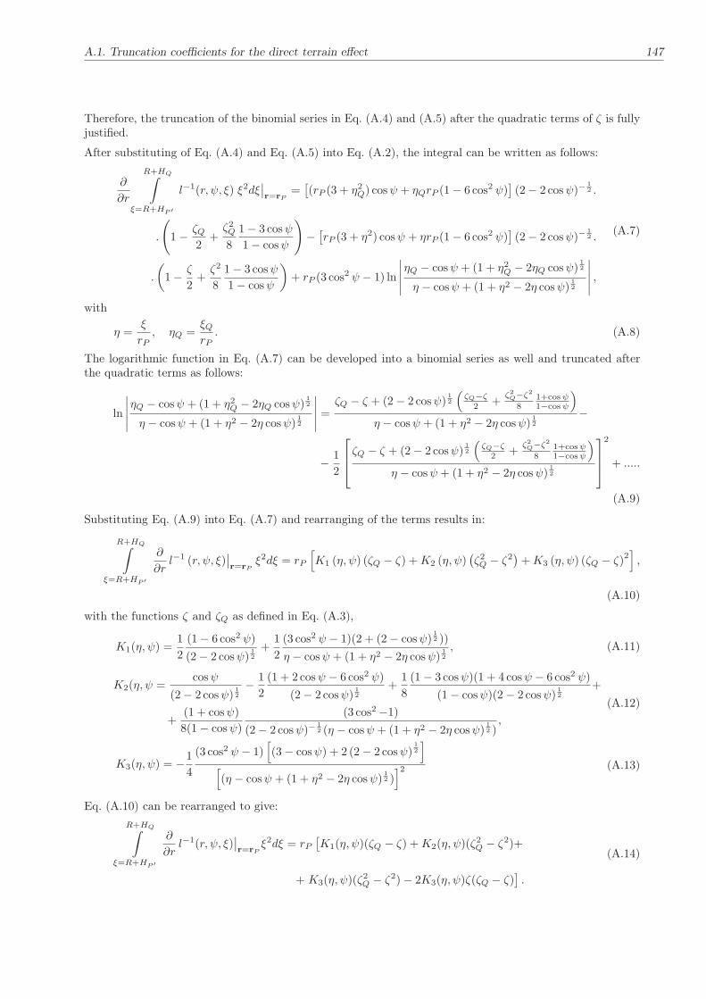
A.1. Truncation coefficients for the direct terrain effect 147
Therefore, the truncation of the binomial series in Eq. (A.4) and (A.5) after the quadratic terms of ζ is fullyjustified.
After substituting of Eq. (A.4) and Eq. (A.5) into Eq. (A.2), the integral can be written as follows:
∂
∂r
R+HQ∫
ξ=R+HP ′
l−1(r, ψ, ξ) ξ2dξ∣∣r=rP
=[(rP (3 + η2
Q) cosψ + ηQrP (1 − 6 cos2 ψ)](2 − 2 cosψ)−
12 .
.
(
1 − ζQ2
+ζ2Q
8
1 − 3 cosψ
1 − cosψ
)
−[rP (3 + η2) cosψ + ηrP (1 − 6 cos2 ψ)
](2 − 2 cosψ)−
12 .
.
(
1 − ζ
2+ζ2
8
1 − 3 cosψ
1 − cosψ
)
+ rP (3 cos2 ψ − 1) ln
∣∣∣∣∣
ηQ − cosψ + (1 + η2Q − 2ηQ cosψ)
12
η − cosψ + (1 + η2 − 2η cosψ)12
∣∣∣∣∣,
(A.7)
with
η =ξ
rP, ηQ =
ξQrP. (A.8)
The logarithmic function in Eq. (A.7) can be developed into a binomial series as well and truncated afterthe quadratic terms as follows:
ln
∣∣∣∣∣
ηQ − cosψ + (1 + η2Q − 2ηQ cosψ)
12
η − cosψ + (1 + η2 − 2η cosψ)12
∣∣∣∣∣=ζQ − ζ + (2 − 2 cosψ)
12
(ζQ−ζ
2 +ζ2Q−ζ2
81+cosψ1−cosψ
)
η − cosψ + (1 + η2 − 2η cosψ)12
−
− 1
2
ζQ − ζ + (2 − 2 cosψ)12
(ζQ−ζ
2 +ζ2Q−ζ2
81+cosψ1−cosψ
)
η − cosψ + (1 + η2 − 2η cosψ)12
2
+ .....
(A.9)
Substituting Eq. (A.9) into Eq. (A.7) and rearranging of the terms results in:
R+HQ∫
ξ=R+HP ′
∂
∂rl−1 (r, ψ, ξ)
∣∣r=rP
ξ2dξ = rP
[
K1 (η, ψ) (ζQ − ζ) +K2 (η, ψ)(ζ2Q − ζ2
)+K3 (η, ψ) (ζQ − ζ)
2]
,
(A.10)
with the functions ζ and ζQ as defined in Eq. (A.3),
K1(η, ψ) =1
2
(1 − 6 cos2 ψ)
(2 − 2 cosψ)12
+1
2
(3 cos2 ψ − 1)(2 + (2 − cosψ)12 ))
η − cosψ + (1 + η2 − 2η cosψ)12
, (A.11)
K2(η, ψ =cosψ
(2 − 2 cosψ)12
− 1
2
(1 + 2 cosψ − 6 cos2 ψ)
(2 − 2 cosψ)12
+1
8
(1 − 3 cosψ)(1 + 4 cosψ − 6 cos2 ψ)
(1 − cosψ)(2 − 2 cosψ)12
+
+(1 + cosψ)
8(1 − cosψ)
(3 cos2 −1)
(2 − 2 cosψ)−12 (η − cosψ + (1 + η2 − 2η cosψ)
12 ),
(A.12)
K3(η, ψ) = −1
4
(3 cos2 ψ − 1)[
(3 − cosψ) + 2 (2 − 2 cosψ)12
]
[
(η − cosψ + (1 + η2 − 2η cosψ)12 )]2 (A.13)
Eq. (A.10) can be rearranged to give:
R+HQ∫
ξ=R+HP ′
∂
∂rl−1(r, ψ, ξ)
∣∣r=rP
ξ2dξ = rP[K1(η, ψ)(ζQ − ζ) +K2(η, ψ)(ζ2
Q − ζ2)+
+ K3(η, ψ)(ζ2Q − ζ2) − 2K3(η, ψ)ζ(ζQ − ζ)
].
(A.14)

148 A. Appendix
The integration over the sphere σ in the first term of Eq. (A.1) can be performed by replacing the geocentriccoordinates ϕQ and λQ by the spherical polar coordinates with the pole in the computation point, ψ and α.Then the first term in Eq. (A.1) can be written as
Gρcr
∫∫
σ
R+HQ∫
ξ=R+HP ′
∂
∂rl−1(r, ψ, ξ)|r=rP
ξ2dξdσ = Gρ
π∫
ψ=0
{(HQ −HP ′)K1(η, ψ)+ .
+1
rP(H2
Q −H2P )(K2(η, ψ) +K3(η, ψ)) − 2HP
rP(HQ −HP ) [K2(η, ψ) +K3(η, ψ)]−
−2(HP ′ −HP )
rP(HQ −HP )K3(η, ψ)
}
sinψ dψ
2π∫
0
dα.
(A.15)
By using the technique introduced by Molodenskii el al. (1960), the terms in Eq. (A.15) can be developedinto a spectral form. If only the far zone has to be taken into account, then the kernels Ki(η, ψ), i=1, 2, 3,in Eq. (A.15) have to be redefined as
Ki(η, ψ) =
{0 0 ≤ ψ < ψ0
Ki(η, ψ) ψ0 ≤ ψ ≤ π. (A.16)
The function Ki(η, ψ), being piecewise continuous, may be expanded into a series of Legendre polynomials(zonal spherical harmonics). For example, it holds for the kernel
K1(η, ψ) =
∞∑
n=0
2n+ 1
2tn(η, ψ, ψ0)Pn(cosψ), (A.17)
with the Legendre polynomials Pn of degree n. The coefficients tn(η, ψ, ψ0) are given by Heiskanen andMoritz (1967) in Sec. 1-13 by,
2n+ 1
2tn(η, ψ, ψ0) =
2n+ 1
4π
2π∫
0
π∫
0
K1(η, ψ)Pn(cosψ) sinψdψdα. (A.18)
After integration with respect to α gives
tn(η, ψ, ψ0) =
π∫
ψ=0
K1(η, ψ)Pn(cosψ) sinψdψ. (A.19)
Introducing the definition of Eq. (A.16), tn(η, ψ, ψ0) can be written as
tn(η, ψ, ψ0) =
π∫
ψ=ψ0
K1(η, ψ)Pn(cosψ) sinψdψ. (A.20)
Because of
HQ(ψ, α) =
∞∑
n=0
HnPn(cosψ), (A.21)
with
Hn =2n+ 1
4π
2π∫
0
π∫
ψ=0
HQ(ψ, α)Pn(cosψ) sinψdψdα, (A.22)

A.1. Truncation coefficients for the direct terrain effect 149
the first term of Eq. (A.15) can be expressed as:
∫∫
σ
(HQ −HP ′)K1(η, ψ)dσ = 2π
Nmax∑
n=0
tn(η, ψ, ψ0)Hn(ϕ, λ) − 2πt0(η, ψ, ψ0)HP ′ , (A.23)
where the truncation coefficients tn(η, ψ, ψ0) are given by Eq. (A.20).
Applying this procedure (Eq. (A.16) to Eq. (A.23)) to the other terms in Eq. (A.15), we arrive at:
Gρcr
∫ ∫
σ→σF Z
R+HQ∫
ξ=R+HP ′
∂
∂rl−1(r, ψ, ξ)|r=rP
ξ2dξdσ = 2πGρcr
[Nmax∑
n=0
tn(η, ψ, ψ0)Hn(ϕ, λ)+
+1
rP
Nmax∑
n=0
un(η, ψ, ψ0)H2n(ϕ, λ) − 2HP
rP
Nmax∑
n=0
un(η, ψ, ψ0)Hn(ϕ, λ)−
−2(HP ′ −HP )
rP
Nmax∑
n=0
vn(η, ψ, ψ0)Hn(ϕ, λ)
]
+ C1,
(A.24)
where the truncation coefficients un(η, ψ, ψ0) and vn(η, ψ, ψ0) are given by:
un(ηψ, ψ0) =
π∫
ψ=ψ0
[K2(η, ψ) +K3(η, ψ)]Pn(cosψ)) sinψdψ, (A.25)
vn(η, ψ, ψ0) =
π∫
ψ=ψ0
K3(η, ψ)Pn(cosψ) sinψdψ, (A.26)
and C1 reads
C1 =2πGρcr[−t0(η, ψ, ψ0)HP ′ − u0(η, ψ, ψ0)H
2P ′/rP +
+ 2u0(η, ψ, ψ0)HPHP ′/rP + 2v0(η, ψ, ψ0)HP ′(HP ′ −HP )/rP ] .(A.27)
The truncation coefficients, given in Eqs. (A.20), (A.25) and (A.26), can be calculated numerically by theGauss-Legendre quadrature formula. It reads, e.g, in case of Eq. (A.20) if the integration ranges from 0 to π(ψ0 = 00),
tn(η, ψ, ψ0) =
π∫
ψ=ψ0
K1(ηψ)(Pn(cosψ)) sinψdψ
≈imax∑
i=1
(Pn(cosψi))K1(η, ψi)wi,
=
imax∑
i=1
F (η, ψi)wi.
(A.28)
The factor wi are the corresponding Gauss-Legendre quadrature weights,
wi =2
(1 − x2i )(P
′
imax(xi))2
, (A.29)
where xi = cosψi and P ′
imaxare the first derivatives of the Legendre polynomials with respect to x. The
values ψi are the zeros of the Legendre polynomials used for a specific Gauss-Legendre quadrature formula.

150 A. Appendix
In our case, the integration starts from ψ0 6= 00. Therefore, the zeros of the Legendre polynomials must betransformed as follows:
ψ′
i = a+ bψi, (A.30)
with
a =cosψ0 + cosπ
2, b =
cosψ0 − cosπ
2. (A.31)
Then the truncation coefficients tn(η, ψ, ψ0) are given by the quadratic formula
tn(η, ψ, ψ0) = b
imax∑
i=1
F (η, ψ′
i)wi. (A.32)
The second integral of Eq. (A.1) can be treated analogously as before resulting in
Gρcr
∫∫
σ
R+HQ∫
ξ=R+HP ′
ξ2dξ∂
∂rl−1(r, ψ, R)|r=rP
dσ = Gρcr
∫∫
σ
[ξ3
3
]R+HQ
R+Hp′
K4(R+HP , ψ,R) sinψ dψdα,
= Gρ
∫∫
σ
[1
3
((R+HQ)3 − (R+HP ′)3
)]
K4(R+HP , ψ,R) sinψdψdα,
= Gρ
∫∫
σ
R3
3
[3(HQ −HP ′)
R+
3(H2Q −H2
P ′)
R2+o
H3
R3
]
K4(R+HP , ψ,R) sinψ dψdα,
(A.33)
where the integral kernel K4(R+HP , ψ,R) is the radial derivative of the Newtonian kernel given by:
K4(R+HP , ψ,R) =R(cosψ − 1) −HP
l3. (A.34)
By inserting Eq. (A.34) in Eq. (A.33), the second integral of Eq. (A.1) can be finally written as
Gρcr
∫ ∫
σ→σF Z
R+HQ∫
ξ=R+HP ′
∂
∂rl−1(r, ψ, R)|r=rP
ξ2dξdσ = 2πGρcr
Nmax∑
n=0
wn(HP , ψ, ψ0)Hn(ϕ, λ)+
+1
R
Nmax∑
n=0
wn(HP , ψ, ψ0)H2n(ϕ, λ) + C2,
(A.35)
with
wn(HP , ψ, ψ0) = R2
π∫
ψ=ψ0
K4(R+HP , ψ,R)Pn(cosψ) sinψdψ, (A.36)
and
C2 = 2πGρcr[−w0(HP , ψ, ψ0)HP ′ − w0 (HP , ψ, ψ0)H
2P ′/rP
]. (A.37)
A.1.2 Helmert’s first or generalized method of condensation
The only difference between Helmert’s first and second condensation method is a different calculation ofthe truncation coefficients wn(HP , ψ, ψ0). The integral kernel K4(R + HP , ψ,R − D1) in Helmert’s firstcondensation method is given by:
K4(R+HP , ψ,R−D1) =:∂ (1/l(r, ψ,R−D1)
∂r
∣∣∣∣r=rP
=(R−D1) cosψ − (R+HP )
l3. (A.38)

A.1. Truncation coefficients for the direct terrain effect 151
A.1.3 Airy-Heiskanen model
In this model, the direct terrain effect of the topographic and isostatic masses is given by (Rummel et al.1988):
DTEter∣∣r=rP
=Gρ
∫∫
σ
R+HQ∫
ξ=R+HP ′
∂
∂rl−1(r, ψ, ξ)|r=rP
ξ2dξdσ+
+G∆ρ
∫∫
σ
R−T−tQ∫
ξ=R−T−tP
∂
∂rl−1(r, ψ, ξ)|r=rP
ξ2dξdσ.
(A.39)
The first integral of Eq. (A.39) is derived from Eq. (A.1) and given by Eq. (A.24). Following an analogousprocedure as used for treating Eq. (A.1), the second integral can be derived resulting in
G∆ρ
∫ ∫
σ→σF Z
R−T−tQ∫
ξ=R−T−tP
∂
∂rl−1(r, ψ , ξ)|r=rP
ξ2dξdσ = 2πG∆ρ
[
−Nmax∑
n=0
qn(η, ψ, ψ0)Hn(ϕ, λ)C+
+1
rP
Nmax∑
n=0
rn(η, ψ, ψ0)H2n(ϕ, λ)C2 +
2(HP + T )
rP
Nmax∑
n=0
rn(η, ψ, ψ0)Hn(ϕ, λ)C−
− 2(T + tP +HP )
rP
Nmax∑
n=0
Sn(η, ψ, ψ0)Hn(ϕ, λ)C
]
+ C3.
(A.40)
The coefficients qn(η, ψ, ψ0), rn(η, ψ, ψ0) and sn(η, ψ, ψ0) are calculated based on Eqs. (A.20), (A.25) and(A.26), respectively, with the parameter
η =R− T − tP
rP. (A.41)
The term C3 is given by:
C3 =2πG∆ρcr [Cq0(η, ψ, ψ0)HP ′ − 1
rPr0(η, ψ, ψ0)C
2H2P ′−
− 2(HP + T )
rPr0(η, ψ, ψ0)CHP ′ +
2(T + tP +HP )
rPs0(η, ψ, ψ0) CHP ′ ] .
(A.42)

152
List of Figures
2.1 Newton’s universal law of gravitation, here point mass m1 considered as attracting mass andm2 as attracted one . . . . . . . . . . . . . . . . . . . . . . . . . . . . . . . . . . . . . . . . . 11
2.2 The gravitational field of an extended mass body . . . . . . . . . . . . . . . . . . . . . . . . . 12
2.3 Spherical coordinates for computation and source point . . . . . . . . . . . . . . . . . . . . . 13
2.4 Potential of a material surface . . . . . . . . . . . . . . . . . . . . . . . . . . . . . . . . . . . . 15
2.5 Gravity field and normal field . . . . . . . . . . . . . . . . . . . . . . . . . . . . . . . . . . . . 17
2.6 Relation between the surface of the Earth, the geoid and the reference ellipsoid . . . . . . . . 19
2.7 Flow chart of the geoid determination procedure considering the various topographic-isostaticeffects . . . . . . . . . . . . . . . . . . . . . . . . . . . . . . . . . . . . . . . . . . . . . . . . . 21
2.8 Relation between the surface of the Earth, the telluroid and the reference ellipsoid . . . . . . 23
2.9 Flow chart of the telluroid determination procedure considering the various topographic-isostatic effects . . . . . . . . . . . . . . . . . . . . . . . . . . . . . . . . . . . . . . . . . . . . 25
2.10 Telluroid before and after the reduction of the topographic masses . . . . . . . . . . . . . . . 26
3.1 Approximation of the geoid by an ellipsoid (left) and a sphere (right) . . . . . . . . . . . . . . 35
3.2 Airy-Heiskanen model, left with constant density; several layers right . . . . . . . . . . . . . . 36
3.3 Ideal situation of the topography (left), three layers of topography (middle) and rock equivalenttopography (right) . . . . . . . . . . . . . . . . . . . . . . . . . . . . . . . . . . . . . . . . . . 37
3.4 Airy-Heiskanen isostatic model in planar approximation . . . . . . . . . . . . . . . . . . . . . 38
3.5 Pratt-Hayford compensating model in spherical approximation with constant density . . . . . 40
3.6 Pratt-Hayford compensating model in spherical approximation with laterally variable density 41
3.7 Pratt-Hayford compensating model (constant density) in planar approximation . . . . . . . . 42
3.8 Local and regional compensation . . . . . . . . . . . . . . . . . . . . . . . . . . . . . . . . . . 43
3.9 Bending of a floating plate . . . . . . . . . . . . . . . . . . . . . . . . . . . . . . . . . . . . . . 44
3.10 The indirect effect . . . . . . . . . . . . . . . . . . . . . . . . . . . . . . . . . . . . . . . . . . 44
4.1 Notation used for the definition of a prism . . . . . . . . . . . . . . . . . . . . . . . . . . . . . 49
4.2 Transformation between the edge system of the prism and the local vertical system at thecomputation point . . . . . . . . . . . . . . . . . . . . . . . . . . . . . . . . . . . . . . . . . . 52
4.3 Notation used for the definition of a condensed prism . . . . . . . . . . . . . . . . . . . . . . . 53
4.4 Geometry of the topography in spherical approximation . . . . . . . . . . . . . . . . . . . . . 56
4.5 Local coordinate system . . . . . . . . . . . . . . . . . . . . . . . . . . . . . . . . . . . . . . . 57

List of Figures 153
4.6 Spherical Airy-Heiskanen topographic-isostatic model . . . . . . . . . . . . . . . . . . . . . . . 61
4.7 Spherical Pratt-Hayford topographic-isostatic model . . . . . . . . . . . . . . . . . . . . . . . 62
4.8 Geometry of Helmert’s condensation models . . . . . . . . . . . . . . . . . . . . . . . . . . . . 63
5.1 GEBCO topography for Canadian Rocky Mountains (units in meter) . . . . . . . . . . . . . . 92
5.2 GEBCO topography for Himalaya (units in meter) . . . . . . . . . . . . . . . . . . . . . . . . 92
5.3 ETOPO5 topography for Asia (units in meter) . . . . . . . . . . . . . . . . . . . . . . . . . . 92
5.4 ETOPO5 topography for the Earth (units in meter) . . . . . . . . . . . . . . . . . . . . . . . 93
5.5 Differences between the numerical integration and the analytical computation of the potentialof a Bouguer shell with a thickness of 2500 m (units in m2/s2) . . . . . . . . . . . . . . . . . 94
5.6 Differences between the numerical integration and the analytical computation of the first radialderivative of the potential of a Bouguer shell with a thickness of 2500 m (units in mGal) . . . 95
5.7 Differences between the numerical integration and the analytical computation of the secondradial derivative of the potential of a Bouguer shell with a thickness of 2500 m (units in Eötvös) 95
5.8 Differences between the numerical integration and the analytical computation of the secondhorizontal (xx and yy) derivative of the potential of a Bouguer shell with a thickness 2500 m(units in Eötvös) . . . . . . . . . . . . . . . . . . . . . . . . . . . . . . . . . . . . . . . . . . . 97
5.9 Second derivatives of the potential of a Bouguer shell with a thickness of 2500 m (Eötvös)determined by numerical integration using different discretizations . . . . . . . . . . . . . . . 97
5.10 Geographical grid (red) and Gauss-Legendre grid (blue) . . . . . . . . . . . . . . . . . . . . . 99
5.11 Comparison between simple quadrature and Gauss Legendre quadrature methods (units inmeter) . . . . . . . . . . . . . . . . . . . . . . . . . . . . . . . . . . . . . . . . . . . . . . . . . 100
5.12 Separate contributions of hαnm, h2αnm and h3αnm to the computation of the uncompensatedpotential coefficients . . . . . . . . . . . . . . . . . . . . . . . . . . . . . . . . . . . . . . . . . 101
5.13 Degree variances of different topographic-isostatic models . . . . . . . . . . . . . . . . . . . . 102
5.14 Near-zone direct terrain effect on gravity of the area inside a cap size of ψ0 = 30 for differenttopographic-isostatic models at an altitude of 4 km (units in mGal) . . . . . . . . . . . . . . 104
5.15 Primary indirect effects of Bouguer shells of the topographic masses (units in mGal) . . . . . 105
5.16 Near-zone primary indirect terrain effect on geoid heights of the area inside a cap size ofψ0 = 30 for different topographic-compensation models (units in meter) . . . . . . . . . . . . 106
5.17 Near-zone secondary indirect terrain effect on gravity of the area inside a cap size of ψ0 = 30
for different topographic-isostatic models at the surface of the Earth (units in mGal) . . . . . 107
5.18 Effects of the near-zone terrain masses on the tensor component Vzz at an altitude of 10 kmfor the Airy-Heiskanen model for the Himalaya region (units in Eötvös) . . . . . . . . . . . . 108
5.19 RMS of direct topographical effects at an altitude of 4 km against the cap radius for differenttopographic-isostatic models . . . . . . . . . . . . . . . . . . . . . . . . . . . . . . . . . . . . . 109
5.20 Far-zone direct terrain effect along the 500 latitude for different topographic-isostatic modelsat an altitude of 4 km . . . . . . . . . . . . . . . . . . . . . . . . . . . . . . . . . . . . . . . . 112

154 List of Figures
5.21 Far-zone direct terrain effect along the 500 latitude for different spectral bands of the sphericalharmonic expansion . . . . . . . . . . . . . . . . . . . . . . . . . . . . . . . . . . . . . . . . . 113
5.22 Far-zone direct terrain effect on gravity of the area outside a cap size of ψ0 = 30 for differenttopographic-isostatic models at an aeroplane altitude of 4km (units in mGal) . . . . . . . . . 114
5.23 Far-zone direct terrain effect on gravity of the area outside a cap size of ψ0 = 30 in case ofgeneralized Helmert method (D1 = 32 km) at different altitudes of the computation point(units in mGal) . . . . . . . . . . . . . . . . . . . . . . . . . . . . . . . . . . . . . . . . . . . . 115
5.24 Far-zone primary indirect terrain effect on geoid heights of the area outside a cap size ofψ0 = 30 for different topographic-compensation models (units in meter) . . . . . . . . . . . . 116
5.25 Far-zone secondary indirect terrain effect on gravity of the area outside a cap size of ψ0 = 30
for different topographic-isostatic models at the surface of the Earth (units in mGal) . . . . . 117
5.26 Far-zone direct terrain effects in case of Helmert’s second method of condensation at thesurface of the Earth: (a) formulae in Novàk et al. (2001), (b) from Eq. (4.191), (c) differencesbetween the two methods (units in mGal) . . . . . . . . . . . . . . . . . . . . . . . . . . . . . 118
5.27 Effects of the far-zone terrain on the tensor components Vzz of the area outside a cap size ofψ0 = 30 at an altitude of 10 km for the Airy-Heiskanen model for the Himalaya region (unitsin Eötvös) . . . . . . . . . . . . . . . . . . . . . . . . . . . . . . . . . . . . . . . . . . . . . . . 119
5.28 Effects of the topographic-isostatic masses on the tensor component Vzz at an altitude of 250km for the Airy-Heiskanen model for the Himalaya region; units in Eötvös) . . . . . . . . . . 122
5.29 Direction derivation of the tensor component Vzz in north-south direction at an altitude of250 km (effect of the topographic-isostatic masses on the tensor component Vzz for the Airy-Heiskanen model for the Himalaya region; units in Eötvös/degree) . . . . . . . . . . . . . . . 123
5.30 Direction derivation of the tensor component Vzz in west-east direction at an altitude of 250 km(effect of the topographic-isostatic masses on the tensor component Vzz for the Airy-Heiskanenmodel for the Himalaya region; units in Eötvös/degree) . . . . . . . . . . . . . . . . . . . . . 123
5.31 Effects of the topographic-isostatic masses on the tensor component Vxx at an altitude of 250km for different topographic-isostatic models (units in Eötvös) . . . . . . . . . . . . . . . . . 124
5.32 Effects of the topographic-isostatic masses on the tensor component Vyyat an altitude of 250km for Helmert’s first method of condensation with different depths (units in Eötvös) . . . . 125
5.33 Effects of the topographic-isostatic masses on the tensor component Vzz at an altitude of 250km for different topographic-isostatic models (units in Eötvös) . . . . . . . . . . . . . . . . . 126
5.34 Effects of the topographic-isostatic masses on the tensor component Vzz at an altitude of 250km for generalized Helmert model of condensation with different depths (units in Eötvös) . . 128
5.35 Effects of the topographic-isostatic masses on the tensor component Vxx at an altitude of 250km for different topographic-isostatic models (units in Eötvös) . . . . . . . . . . . . . . . . . 129
5.36 Effects of the topographic-isostatic masses on the tensor component Vyy at an altitude of 250km for different topographic-isostatic models (units in Eötvös) . . . . . . . . . . . . . . . . . 130
5.37 Effects of the topographic-isostatic masses on the tensor component Vzz at an altitude of 250km for different topographic-isostatic models (units in Eötvös) . . . . . . . . . . . . . . . . . 131
5.38 Orbit deviations for different topographic isostatic models (altitude: ∼400 km) . . . . . . . . 133
5.39 SST ranges: EGM96 versus (EGM96-T/I-models) (altitude: ∼ 450 km) . . . . . . . . . . . . 134
5.40 SST range-rates: EGM96 versus (EGM96-T/I-models)(altitude: ∼ 450 km) . . . . . . . . . . 134

155
List of Tables
3.1 Polynomial coefficients of the bended curve . . . . . . . . . . . . . . . . . . . . . . . . . . . . 45
5.1 Differences between the numerical integration and the analytical computation of the potentialof a Bouguer shell with a thickness 2500 m (units in m2/s2) . . . . . . . . . . . . . . . . . . . 95
5.2 Near-zone terrain effects at an altitude of 4 km for Helmert’s first and generalized model ofcondensation with different depths in comparison with Airy-Heiskanen (units in mGal) . . . . 103
5.3 Near-zone direct terrain effects for different altitudes for Helmert’s methods of condensationand Airy-Heiskanen model (units in mGal) . . . . . . . . . . . . . . . . . . . . . . . . . . . . 109
5.4 Far-zone terrain effects at an altitude of 4 km for Helmert’s first and generalized model ofcondensation with different depths in comparison with Airy-Heiskanen (units in mGal) . . . . 109
5.5 Far-zone direct terrain effects for different cap size radii and different altitudes in case ofHelmert’s second method of condensation (units in mGal) . . . . . . . . . . . . . . . . . . . . 110
5.6 Far-zone direct terrain effects for different cap size radii and different altitudes in case of thegeneralized Helmert model of condensation (D1 = 32 km; units in mGal) . . . . . . . . . . . 110
5.7 Statistics of the differences between the numerical integration method and the spherical har-monic expansion on the tensor component at an altitude of 250 km for Airy-Heiskanen model(units in Eötvös) . . . . . . . . . . . . . . . . . . . . . . . . . . . . . . . . . . . . . . . . . . . 122
5.8 Effects of the topographic-isostatic masses on the tensor component at an altitude of 250 kmfor Helmert’s first or generalized method of condensation with different depths in comparisonwith Airy-Heiskanen and Pratt-Hayford models (units in Eötvös) . . . . . . . . . . . . . . . . 127

INFORMATION ABOUT THE AUTHOR
Atef Abdel-Hakeem Makhloof was born on 5 of January 1970 in El-Minia, Egypt. Between 1976 and 1982he visited the primary school in Edmo and from 1982 to 1985 he visited the preparatory school in Demshir.From 1985 till 1988 he visited the Secondary school in Minia. After five years and in 1993 he got his B.Sc.in Civil Engineering from the Faculty of Engineering at Minia, Minia University. From 1993 to 1997 he gothis M.Sc. in the field of civil engineering from the Faculty of Engineering at Minia, Minia University. Fromthe period of 1997 to 2002 he worked as assistant lecturer in the Faculty of Engineering at Minia, MiniaUniversity. From the period of 2002 to 2006 he is a Ph.D student in the institute of the theoretical geodesy,Bonn University, Germany. The address of the author isCivil Engineering departementFaculty of EngineeringMinia universityMiniaEgyptEmail address: [email protected]