the use of heuristics and exposure models in improving

TheUseofHeuristicsandExposureModelsinImprovingExposureJudgmentAccuracy

A Dissertation

SUBMITTED TO THE FACULTY OF

UNIVERSITY OF MINNESOTA

BY

Susan F. Arnold

IN PARTIAL FULFILLMENT OF THE REQUIREMENTS

FOR THE DEGREE OF

DOCTOR OF PHILOSOPHY

Gurumurthy Ramachandran, Ph.D.

September, 2015

i

ACKNOWLEDGEMENTS

My most sincere gratitude is extended to my advisor, Dr. Gurumurthy Ramachandran

whose curiosity, creative thinking and sense of humor were instrumental in bringing this

research to fruition and completion.

I am so grateful to my committee, Dr. Pete Raynor, whose constructive input made this

work more robust and to Dr. Sudipto Banerjee for his statistical guidance. My thanks are

also extended to Dr. Perry Logan for helping to brainstorm project ideas, offer helpful

feedback and recruit volunteers, a crucial step in this work.

Thanks to Mark Stenzel, whose heuristics and algorithms played a central role in this

work and for sharing his extensive knowledge relating to solvent exposures. Thanks to

Yuan Shao for his thoughtful questions and input and help in the lab.

Thank you to Dr. Bruce Alexander for his support and sage advice and to the staff who

helped me navigate my way as a new student and Minnesota resident. Special thanks go

out to Karen Brademeyer, Debb Grove, Khosi Nkosi, Frank Strahan and Simone Vuong.

My heartfelt thanks are also extended to my husband for his tactical assistance and loving

and unfailing support.

ii

Lastly, I am so grateful to the many volunteers who contributed to the development of

exposure scenarios, execution of expert elicitation workshops and the many study

participants whose exposure judgment data were essential to this learning.

iii

DEDICATION

This dissertation is dedicated to my family, especially my husband, Steve. It’s been an

incredible journey and so much more so because you were a part of it.

iv

TABLEOFCONTENTS

ContentsThe Use of Heuristics and Exposure Models in Improving ................................................. i

ACKNOWLEDGEMENTS ................................................................................................. i

DEDICATION ................................................................................................................... iii

TABLE OF CONTENTS ................................................................................................... iv

Contents ............................................................................................................................. iv

List of Tables .................................................................................................................... vii

List of Figures ..................................................................................................................... x

CHAPTER 1 INTRODUCTION – INVESTIGATING INPUTS TO ACCURATE DECISION MAKING .................................................................................................. 1

BACKGROUND AND SIGNIFICANCE ...................................................................... 1

Low accuracy of professional judgments relating to exposure: ...................................... 1

Exposure Heuristics: ..................................................................................................... 10

Aids to decision making: Use of algorithms (checklists) and models .......................... 12

Exposure Models: ......................................................................................................... 13

Selecting commonly used occupational exposure physical models ............................. 14

Box Models ............................................................................................................................ 15

Impacts on occupational exposure assessment and Research-to-Practice (R2P): ........ 19

Innovation: .................................................................................................................... 21

Specific Aims of this Research ..................................................................................... 21

CHAPTER 2. USING CHECKLISTS AND ALGORITHMS TO IMPROVE

QUALITATIVE EXPOSURE JUDGMENT ACCURACY ............................................ 28

INTRODUCTION ............................................................................................................ 28

v

METHODS ....................................................................................................................... 31

The Rule of 10 .............................................................................................................. 32

Vapor Hazard Ratio ...................................................................................................... 32

Particulate Hazard Ratio ............................................................................................... 32

The Checklist ................................................................................................................ 32

Eliciting IH exposure judgments using the Checklist ................................................... 34

Evaluating Exposure Judgments ................................................................................... 36

RESULTS ......................................................................................................................... 39

DISCUSSION ................................................................................................................... 42

CONCLUSIONS............................................................................................................... 48

ACKNOWLEDGMENTS ................................................................................................ 49

CHAPTER 2 EVALUATING WELL MIXED ROOM AND NEAR FIELD FAR FIELD MODEL PERFORMANCE UNDER HIGHLY CONTROLLED CONDITIONS ............................................................................................................. 50

INTRODUCTION ............................................................................................................ 50

METHODS ....................................................................................................................... 52

Chamber Design and Construction ............................................................................... 54

Chamber Study Design ................................................................................................. 55

Chamber Study Design for the NF-FF Model Evaluation ............................................ 62

Model Evaluation Criteria ............................................................................................. 64

RESULTS ......................................................................................................................... 69

Model Evaluation – WMR model ................................................................................. 69

Model Evaluation – NF-FF Model ............................................................................... 73

DISCUSSION ................................................................................................................... 78

CONCLUSION ................................................................................................................. 83

ACKNOWLEDGMENTS ................................................................................................ 83

CHAPTER 3 EVALUATION OF FUNDAMENTAL EXPOSURE MODELS IN OCCUPATIONAL SETTINGS ................................................................................. 84

INTRODUCTION ............................................................................................................ 84

vi

METHODS ....................................................................................................................... 85

Model Description ........................................................................................................ 85

The Models ................................................................................................................... 87

Model Evaluation Criteria ........................................................................................... 102

RESULTS ....................................................................................................................... 105

DISCUSSION ................................................................................................................. 113

CONCLUSION ............................................................................................................... 121

CHAPTER 4 SCENARIOS ...................................................................................... 123

Scenarios 3 and 4. Using physical chemical models to estimate respirable dust and silica from sanding drywall in new construction environment .................... 130

Scenario 5. And 6. Using physical chemical models to estimate cobalt exposure while weighing Lithium Cobalt Oxide powder, and mixing through cleaning tasks in a clean room area. .................................................................... 134

Scenario 7. Using physical chemical models to estimate exposure to methylene chloride: .................................................................................................. 140

Scenario 8. Using physical chemical models to estimate phenol exposure while making sand molds containing a phenolic resin .................................................. 143

Scenario 9. Using physical chemical models to estimate a salon professional’s exposure to acetone in a nail salon: ...................................................................... 146

Scenario 10. Using physical chemical models to estimate acetone exposure while cleaning the lid and blades of a Morehouse mixer ................................... 150

CHAPTER 5 CONCLUSIONS AND FUTURE DIRECTION ............................ 154

OVERALL CONCLUSIONS ......................................................................................... 154

Limitations of the Study and Future Directions .......................................................... 164

BIBLIOGRAPHY ........................................................................................................... 167

APPENDIX I .................................................................................................................. 172

APPENDIX II ................................................................................................................. 183

Well Mixed Room Model ........................................................................................... 183

Near Field Far Field Model ......................................................................................... 184

vii

ListofTables

Table 1-1 AIHA Exposure Category Rating Scheme ......................................................... 2

Table 2-1 Solvent Properties of the three solvents used in the chamber study ................. 55

Table 2-2Generation Rates and Ventilation Rate Ranges ................................................. 56

Table 2-3 Sampling locations in the chamber relative to the contaminant source for the

WMR tests ........................................................................................................................ 57

Table 2-4 Reported (Dräger Safety AG & Co. KGaA) and observed Response Factors . 59

Table 2-5 Framework showing AIHA Exposure Control Categories (ECC) and

recommended statistical interpretation ............................................................................. 67

Table 3-1 Model inputs and output for the WMR and (additional) inputs required for the

NF-FF model. .................................................................................................................... 90

Table 3-2 Summary Describing Field Scenario Tasks, Agents and Exposure Limits

included in the Model Evaluation. .................................................................................... 96

Table 3-3 Model inputs for each scenario, including distributions and ranges used to

apply models probabilistically. LN: Log normal distribution with (Geometric Mean, GM,

and Geometric Standard Deviation, GSD). U: Uniform distribution with (minimum,

maximum) values. ........................................................................................................... 101

Table 3-4 Framework showing AIHA Exposure Control Categories (ECC) and

recommended statistical interpretation for each category. Using this framework, model

performance was evaluated categorically. ...................................................................... 105

viii

Table 3-1 Performance evaluation criteria and scores in accordance with ASTM 5157

using time-varying measured and modeled exposure estimates from the WMR and NF FF

models, respectively for six scenarios. ........................................................................... 106

Table 4-1S Calculating the Near Field flow rate from the face velocity and area

measurements .................................................................................................................. 125

Table 4-2S Calculating an average G for each source from C measured at each source.

An overall average G is calculated from these average values. ...................................... 127

Table 4-3S An average G is calculated for each of the four sources, as well as an overall

average G. ....................................................................................................................... 127

Table 4-4S Calculating G for each test by back-calculating from the concentration

generated under highly controlled conditions. ................................................................ 131

Table 4-5S Calculating the Generation rate from the Near Field Concentration, the value

obtained directly over the source (G4) to estimate the upper bound G .......................... 135

Table 4-6S Estimating G from Source Sampling ......................................................... 137

Table 4-7S Calculating G from C for each manicure. ................................................... 147

Table 4-8S Back calculating from C to estimate G. The average generation rate was

1638.2 mg/min. ............................................................................................................... 151

Table 5-1 AIHA Exposure Control Categories (ECC) with criteria for interpretation ... 175

Table 5-2 Rule of 10 Engineering Control Matrix .......................................................... 176

Table 5-3 Vapor Hazard Ratio (VHR) Engineering Control Matrix .............................. 177

Table 5-4 Particulate Hazard Ratio (PHR) Engineering Control Matrix ....................... 178

Table 5-5 The Checklist - an ordered approach to applying the three heuristics ........... 179

ix

Table 5-6 Exposure Scenario Details, showing the Scenario number, agent of concern

(Chemical Agent), the relevant OEL , the primary task or work process from which the

exposure occurred (Process), the number of personal exposure samples collected, from

which the Reference ECC was calculated (Reference ECC data set) and the

corresponding Reference ECC. ....................................................................................... 179

Table 5-7a Results from novice IHs’ exposure judgments, showing bias (the difference

between the average predicted ECC and reference ECC), and Precision (standard

deviation) for each scenario (n = 8) ................................................................................ 181

Table 5-8 Exposure Scenario using the OEL as the benchmark, OEL = 10 ppm, GSD =

2.5.................................................................................................................................... 182

x

ListofFigures

Figure 1-1 Example qualitative exposure judgment chart illustrating an occupational

hygienist’s exposure judgment given the information and data available .......................... 4

Figure 1-2 (a) Percentage of all pre- and post-training quantitative task judgments above,

below and reference categories for (a) desktop study, N = 3834, (Logan et al., 2009) ...... 6

Figure 1-3 (a): Percentage of all pre- and post-training qualitative task judgments above,

below and reference categories for (a) desktop study, N = 552, (Logan et al., 2009) ........ 8

Figure 1-4 Schematic Diagram of the two-compartment or two-zone model .................. 17

Figure 2-1a Schematic of WMR model ............................................................................ 53

Figure 2-2 Measuring Q from concentration decay data .................................................. 58

Figure 2-3 Full size exposure chamber arrangement for WMR studies ........................... 61

Figure 2-4 Exposure Chamber – NF/FF Configuration showing arrangement in the

chamber for the NF-FF model. FF sampling locations correspond to WMR sampling

locations 4, 5 and 6, respectively. ..................................................................................... 64

Figure 3-1 Schematic of the WMR Model, with a non-point source generating an airborne

concentration and air that is well mixed so that the contaminant concentration in the air is

uniform throughout the room. ........................................................................................... 87

Figure 3-2 Schematic of the NF-FF Model with a point-source generating an airborne

contaminant concentration, resulting in a concentration that is greater immediately

surrounding the source. Air in each of the NF and FF are well mixed, but air moving

between the two boxes, denoted by ß is limited. .............................................................. 89

Figure 3-3 Measuring Q from concentration decay data .................................................. 93

xi

Figure 3-4 Application of the NF FF model to the slurry pot lid cleaning task defining the

NF as a hemisphere, encompassing the source and the technician’s breathing zone. ...... 99

Figure 3-1a and b Measured and modeled time varying acetone concentration from slurry

pot lid cleaning collected on day 4, using the WMR andNF FF models. ....................... 108

Figure 3-2 Comparison of Modeled and measured Cobalt (mg/m3) for weighing and

mixing tasks, respectively. .............................................................................................. 111

Figure 3-3 Categorical accuracy of each model relative to random chance. ................. 112

Figure 5-1 Bayesian Decision Chart, showing the IHs belief that the 95th percentile of the

exposure distribution for a given scenario most likely belongs to Exposure Control

Category (ECC) 4. .......................................................................................................... 172

Figure 5-2 Categorical Judgment Accuracy, showing accuracy attributable to random

chance pre-training (Baseline), post-training Checklist-guided judgment accuracy for

Novices and practicing IHs. ............................................................................................ 173

Figure 5-3Baseline and Checklist based judgment accuracy for Novice IHs ................. 174

1

CHAPTER1 INTRODUCTION–INVESTIGATINGINPUTSTOACCURATEDECISIONMAKING

BACKGROUND AND SIGNIFICANCE

Low accuracy of professional judgments relating to exposure:

Exposure assessments provide the foundation for determining whether occupational and

environmental exposure risks are efficiently and effectively managed. Most exposure

assessment strategies require the workforce to be categorized into similar exposure

groups or SEGs. The American Industrial Hygiene Association’s (AIHA) strategy is

well-known and provides a simple yet elegant framework for exposure assessments (Jahn

et al., 2015; Ignacio and Bullock, 2006; Mulhausen and Damiano, 1998). Judgments are

made by identifying the exposure control category in which the 95th percentile of the

exposure distribution is most likely located for a given job or task (Table 1-1).

Acceptability is commonly evaluated by comparing the true group 95th percentile to the

occupational exposure limit (OEL), and based on this comparison the exposure is

classified into one of four categories: “highly-controlled”, “well controlled”,

“controlled”, or “poorly controlled”. A judgment can be documented for each SEG,

which can represent a single task that may be short in duration or may represent a group

of tasks that comprise a full-shift exposure. Qualitative and quantitative exposure

assessments are performed after a thorough review of available information and data

related to the workforce, jobs, materials, worker interviews, exposure agents, exposure

limits, work practices, engineering controls and protective equipment.

2

Table1‐1AIHAExposureCategoryRatingScheme

A SEG is assigned an exposure rating by comparing the 95th percentile exposure distribution (X0.95) with the full-shift time-weighted average (TWA), Occupational Exposure Limit (OEL) or Short-Term Exposure Limit (STEL) to determine in which category it most likely falls.

AIHA

Exposure

Rating

Proposed

Control Zone

Description

General Description AIHA-Recommended

Statistical Interpretation

1

Highly

Controlled

(HC)

95th percentile of exposures rarely

exceeds 10% of the limit. X0.95 < 0.10 OEL

2

Well

Controlled

(WC)


exceeds 50% of the limit.

0.10 OEL < X0.95 <

0.5 OEL

3 Controlled

(C)


exceeds the limit.

0.5 OEL < X0.95 <

OEL

4

Poorly

Controlled

(PC)

95th percentile of exposures exceeds

the limit. OEL < X0.95

Exposure judgments are commonly used in a wide range of situations, including

retrospective exposure assessments for epidemiology studies (e.g. Esmen et al., 1999;

Ramachandran, 2001; Ramachandran et al., 2003; Friesen et al, 2003) and current and

prospective exposure assessments for managing exposures related to consumer use and

3

manufacturing operations, (e.g. Hawkins and Evans, 1989; Teschke et al., 1989;

Macaluso, 1993; Friesen et al., 2003; Ramachandran et al., 2003). When there are limited

sampling data, occupational hygienists (OHs) use a combination of professional

judgment, personal experience with a given operation, and review of exposures from

similar operations to assess the acceptability of exposures for managing engineering

controls, medical surveillance, hazard communication and personal protective equipment

programs (Teschke et al., 1989; de Cock et al., 1996; Burstyn & Teschke, 1999; Friesen,

2003; Kolstad, et al., 2005; Logan et al., 2009; 2011; Vadali et al., 2011; 2012). In the

context of this work, a decision is represented by a chart showing the hygienist’s

assessment of the probabilities that the 95th percentile lies in each of the four categories

(Figure 1-1).

4

Figure1‐1Examplequalitativeexposurejudgmentchartillustratinganoccupationalhygienist’sexposurejudgmentgiventheinformationanddataavailable

This chart shows that the hygienist is highly confident the 95th percentile falls into Category 4 – >100 of the OEL (Arnold and Ramachandran, 2015)

A number of studies have been published on the accuracy of professional judgments

(Kahneman et al., 1982; Kromhout, et al., 1987; Glaser & Chi, 1988; Teschke, et al.,

1989; Hawkins & Evans, 1989; Macaluso et al., 1993). Recent studies (Logan et al.,

2009; Logan et al., 2011; Vadali, et al. 2011; Vadali et al., 2012) involved both desktop

assessments (where participating OHs viewed videos of tasks, task information and

sampling data) and walkthrough assessments (where they directly observed the task). The

key findings relating to quantitative judgments (made using monitoring data) shown in

Figure 1-2a and 1-2b are:

Pro

babi

lity

of

the

95th

per

cent

ile

bein

g lo

cate

d in

an

expo

sure

con

trol

cat

egor

y

5

• The accuracy of exposure judgments made by hygienists when monitoring

data are available is low (<50% correct judgments) but still better than

random chance (25%).

• There is a significant underestimation bias in the exposure judgments, i.e.,

there is marked tendency to assign a lower exposure category than the

correct one, thus increasing occupational risk to workers.

• The low accuracy is likely due to cognitive biases in understanding skewed

lognormal distributions. A training focused on heuristics relating to

lognormal statistics significantly improves accuracy to ~70%.

• Several factors relating to cumulative professional experience, training,

certification, and educational level of the hygienists, as well as task-specific

experience were significant predictors of judgment accuracy.

6

Figure1‐2(a)Percentageofallpre‐andpost‐trainingquantitativetaskjudgmentsabove,belowandreferencecategoriesfor(a)desktopstudy,N=3834,(Loganetal.,2009)

7

Figure1‐2(b)Percentageofallpre‐andpost‐trainingquantitativetaskjudgmentsabove,belowandreferencecategoriesforwalkthroughstudy,N=2142

Thisfigureshowsthedeviationofparticipants’quantitativejudgmentspreandposttrainingfromrandomchance,(Vadalietal.,2012b).

The findings related to qualitative judgments (when no monitoring data are available)

shown in Figures 3a and 3b are:

• The accuracy of exposure judgments made by hygienists when monitoring data are not

available (30%) is not much different from random chance (25%).

• The underestimation bias is significant in this case as well.

8

Figure1‐3(a):Percentageofallpre‐andpost‐trainingqualitativetaskjudgmentsabove,belowandreferencecategoriesfor(a)desktopstudy,N=552,(Loganetal.,2009)

9

Figure1‐3(b)Percentageofallpre‐andpost‐trainingqualitativetaskjudgmentsabove,belowandreferencecategoriesforworkplacewalkthroughstudy,N=93.

Thisfigureshowsthedeviationofparticipantsqualitative’judgmentspre‐trainingfromrandomchance,(Vadalietal.,2012b).

It is this second set of findings relating to qualitative judgment accuracy (Figure 1-3a, b)

that motivated this research, although the quantitative accuracy findings (Figure 1-2a, b)

are related as well.

The vast majority of the exposure judgments made by practitioners are qualitative and in

many cases even determine if any measurements should be made. The low accuracy of

these judgments can therefore lead to incorrect follow-up activities, and is therefore a

cause for concern. These findings suggest that the understanding of how workplace

factors affect exposure needs to be significantly improved among practitioners (Burstyn

10

and Teschke, 1999; Hawkins & Evans, 1989). Statistical training, being unrelated to

decision-making when there are no data, did not improve accuracy. However, we

hypothesized that there are other types of training that may be relevant and could improve

accuracy, including Exposure Determinants Heuristics (EDH) and exposure modeling

training.

Exposure Heuristics:

Mental shortcuts, known as heuristics, are often used when information or data are

insufficient or absent, making the decision process efficient but can lead to errors in

judgment and introduce bias. Using these heuristics leads to a pattern that, when faced

with uncertain prospects, assigns weights to our decisions that differ from the true

probabilities of these outcomes. Improbable outcomes are over-weighted, while almost-

certain outcomes are under-weighted.

In their research on decision making, Kahneman et al., (1982) found these cognitive

biases could frequently be attributed to three heuristics: availability, representativeness,

and anchoring and adjustment. The availability heuristic reflects the tendency to equate

the probability of an event with the ease with which an occurrence can be retrieved from

our memory. The degree to which a person’s experiences and memory matches the true

frequency determines whether these judgments are accurate. Representativeness reflects

assignment of an object or event to a specific group or class of events. If the decision

maker lacks relevant experience, a surrogate (and less relevant) memory may be used,

leading to erroneous conclusions. The anchoring and adjustment heuristic is a strategy for

11

estimating uncertain quantities. When trying to determine the correct value, our minds

‘anchor’ on a value, and then adjust to accommodate additional information. The degree

to which our final answer is anchored to the initial value can be influenced by many

factors. For example, when tired or when our mental resources are spent, we tend to stay

closer to the initial value. Within the realm of industrial hygiene decision making, there

are many situations where these heuristics can be identified, such as judgments based

solely on the “available” information in one’s memory. The representativeness heuristic

might be invoked when “eyeballing” exposure data, making a judgment modeled on a

symmetrical (normal) distribution (which our minds more readily intuit) rather than the

skewed, lognormal distribution that more closely reflects most exposure profiles. By

modeling the data after a symmetrical, rather than a skewed distribution, the hygienist is

likely to underestimate the decision statistic, and consequently underestimate the true

exposure. Similarly, when a hygienist ‘anchors on a single piece of information’,

neglecting to take into consideration the most critical factors before making an exposure

judgment can lead to erroneous conclusions.

Objective, structured approaches, using simple algorithms and exposure modeling are

more resistant to these vulnerabilities, focusing the decision maker on the decision

making process, and on the critical inputs, while filtering out nonessential information.

These approaches have been shown to improve decision making across a broad range of

domains, including psychology (Kahneman, 2011 and Kahneman et al., 1982), drug

delivery and development (Lipinski et al., 2001); redicting transdermal delivery and

12

toxicity (Magnusson et al., 2004;) environmental exposure assessment ( Fristachi et al.,

2009); and aggregate exposure assessment (Cowan-Ellsberry and Robinson, 2009).

These same objective approaches can be applied to occupational exposure assessment. In

fact, decisions are most accurate in highly uncertain ‘low validity’ environments, i.e.

situations with little or no data, when the final decision is generated from algorithms. The

Apgar test is an excellent example. This algorithm, capturing a pattern of behaviors

recognized by obstetrical anesthesiologist Virginia Apgar, considers just five basic

inputs, with a score assigned to each. The sum of the scores corresponds to the baby’s

health prognosis. First reported in 1952, this algorithm was better able to predict when

medical assistance was needed than individual experts, (Apgar, 1958, Gawande, 2010)

and is the still the standard in assessing a newborn’s transition to life outside the womb.

Aids to decision making: Use of algorithms (checklists) and models

Algorithms consider critical and consistent inputs and are consistently better at making

accurate judgments, while experts try to out-finesse algorithms, thinking outside the box,

considering complex combinations of inputs (Meehl, 1954). Humans, however, are

inconsistent in making summary judgments of complex information and are therefore less

consistent, and less accurate. (Kahneman, 2010) The algorithms may not be optimal or

100% accurate, but are close enough to be informative and ensure limited resources are

used efficiently. Subjective intuitive qualitative judgments are, most of the time, no more

accurate than random chance (Arnold et al., 2015; Logan, et al., 2011; Vadali et al., 2011;

Vadali et al., 2012). Identifying and applying proven aids to decision making, is essential

13

to ensuring these exposure judgments are highly accurate and health conservative.

One of the characteristics of algorithms and models contributing to consistent decision

making is the consistent order in which information is processed. Checklists provide

guidance on the order in which inputs are considered. These simple tools have been the

cornerstone of safety excellence in the aviation industry for years. That is not to say that

checklists and models do not replace knowledge and expertise, and pilots go through

rigorous training before they are allowed to fly. The checklists ensure they follow the

critical steps at the right time to ensure theirs, and their passengers’ safety. Likewise,

checklists may help OHs focus on the critical inputs to decision making in the right order,

leading to consistent and accurate exposure judgments, protecting the health and safety of

those in their care.

Exposure Models:

Models have been applied across a broad range of fields to improve decision making,

from weather forecasting to medical diagnosis and treatment selections (Kahneman,

2011). Meehl (1954) asserted that models consistently produce significantly more

accurate judgments than subjective expert judgments. The nearly 200 studies conducted

since this evidence was first published support this assertion (Kahneman, 2011). The

range of predicted outcomes has expanded to include economic indicators, career

satisfaction of workers, questions of interest to government agencies and the future price

of Bordeaux wines. Pharmaceutical researchers use simple models based on readily

available inputs, identifying potential candidate compounds for transdermal drug

14

(Magnusson et al., 2004) and oral drug delivery (Lipinski et al., 2011). The Apgar test, a

simple model comprised of five critical determinates has been helping save the lives of

neonates since 1953 (Kahneman, 2011). These fields have in common a significant

degree of uncertainty and unpredictability, which Kahneman (2011) refers to as ‘low-

validity’. The application of models to the low-validity field of occupational hygiene

exposure risk assessment is a logical next step towards improving exposure judgments.

Exposure models have tremendous potential for improving the efficiency and

effectiveness of risk assessment and management programs. They can be used to predict

exposures for operations that have not yet been installed or to reconstruct exposures for

processes that have long disappeared, or when monitoring data are impossible or

expensive to generate. They can enrich and inform qualitative exposure judgments and

offer potential for increasing judgment accuracy. The physical models employed today in

occupational hygiene are typically based upon some simplifying assumptions about air-

flow and contaminant transport pattern (Hemeon, 1963; Nicas, 1996; Keil et al., 2009).

Predicting exposure in real settings is constrained by lack of quantitative knowledge of

exposure determinants (Keil and Murphy, 2006; Arnold et al., 2009; Cherrie et al., 1999;

Jones et al., 2011; Earnest and Corsi, 2013).

Selecting commonly used occupational exposure physical models

There are several deterministic models with varying levels of sophistication

(Ramachandran 2005; Arnold, et al., 2009) and correspondingly varying costs due to the

15

amount of information needed as model inputs. For example, the near field-far field

model requires knowledge of room ventilation and contaminant generation rates in

addition to a parameter known as the inter-zonal ventilation rate – involving a non-trivial

investment. A sophisticated eddy diffusion model, which accounts for concentration

gradients around pollution sources, requires even greater investments. While costs

increase with the level of sophistication, more complex models can also yield more

refined exposure estimates. Two commonly referenced physical models are briefly

outlined here – a more complete listing is provided in Keil et al. (2009). These models are

applicable to both gas/vapor as well as aerosol contaminants, by proper choice of some

model parameters.

Box Models

The one-compartment model

This model assumes that (a) a source is generating an airborne pollutant at a rate G

(mg/hour) in a room of volume V (m3) with a ventilation rate Q (m3/hour), and (b) the air

in the room is perfectly mixed creating a uniform contaminant concentration throughout

the room, irrespective of the distance from the source. A loss rate coefficient, kL, governs

mechanisms (other than ventilation) by which the pollutant is removed from the room.

Examples of such mechanisms include adsorption of gases and vapors onto various

surfaces (here kL is an adsorption rate for the particular vapor and surface type) and

particle deposition on surfaces by gravitational settling (kL is now a function of terminal

settling velocity for particles of a given diameter and density), impaction, and Brownian

16

diffusion. Thus, kL helps generalize this model to gaseous as well as particulate air

contaminants. The differential equation describing this model is:

, (1-1)

where CIN is the concentration in the incoming air. The steady state concentration for this

scenario is

(1-2)

in mg/m3.

Therefore, the input parameters required for this model are the generation and ventilation

rates, the room volume, and the loss rate parameter that is a function of contaminant

physical properties.

The two-compartment or two-zone model

The near field far field (or two-zone) model assumes that (a) a contamination source is

present in the workplace, (b) the region very near and around the source is one well-

mixed box, called the near field, while the rest of the room is another well-mixed box,

called the far field, which completely encloses the near field box, (c) there is air exchange

between the two boxes with airflow rate equal to β, (d) the contaminant’s total mass is

emitted at rate G, and (e) the supply and exhaust flow rates are both equal to Q. The kL

refers to contaminant loss by other mechanisms as described earlier.

17

Figure1‐4SchematicDiagramofthetwo‐compartmentortwo‐zonemodel

Figure 1-4 schematically depicts the system, where VN and VF denote the volumes at the

near and far field, respectively. In this context, the occupational hygienist seeks to model

the exposure concentrations at the near and far fields based upon observations collected

over a period of time. The mass balance for the two zones, ignoring kL since its

contribution is de minimis, is given by:

VNFdCNF = [Gdt + CFFdt] CNFdt (1-3)

VFFdCFF = CNFdt [CFFdt + QCFFdt] (1-4)

This gives a pair of coupled differential equations that can be solved to yield the near-

field and far-field concentrations as a function of time. The solutions are of the form

)exp()exp( 2211 ttCNF (1-5)

)exp()exp( 2413 ttCFF (1-6)

where αi is

18

(1-7)

And λi is

(1-8)

Traditionally, subjective judgments made with little transparency have driven most

exposure judgments, (Logan and Hewett, 2009), while direct measurements have played

a less conspicuous role. Recent studies (Logan et al., 2009; Vadali, et al. 2012; Vadali et

al., 2012) have shown that the accuracy of judgments made by occupational hygienists

(OHs), when small numbers of monitoring data are available is rather low (~40-45%).

Exposure modeling, which has been shown to improve decision making across a broad

range of domains, (Kahneman et al., 1982; Lipinski, et al., 2001; Magnusson et al.,, 2004;

Fristachi et al. 2009; Cowan-Ellsberry & Robison, 2009; Jones et al., 2011; Kahneman,

2011) provides a systematic and transparent approach for making exposure judgments but

has received little support from industry and government. Guidance directing OHs on

which model would produce the most accurate exposure estimate under a defined set of

conditions is needed – and for this, the models need to be systematically evaluated in

both chamber and field environments. OHs also lack training opportunities providing

immediate feedback on their judgment accuracy, allowing them to calibrate their

judgment based on these exposure models. Lacking this training experience, OHs may

undervalue models as tools for making accurate exposure judgments and therefore

19

underutilize them. However, this situation is changing dramatically with the advent of the

REACH regulations in the EU that requires assessing exposures in a variety of exposure

scenarios where monitoring may not be feasible.

Exposure models seek to capture the underlying physical processes generating chemical

concentrations in the workplace. An accurate representation will produce better

concentration estimates and facilitate decision-making in exposure management.

However, this is challenging because workplaces are notoriously complex and no

physical model is likely to provide a complete representation. Thus, characterizing model

parameters, and accounting for parameter and model uncertainty is crucial.

Impacts on occupational exposure assessment and Research-to-Practice (R2P):

The work conducted falls under the NIOSH Cross-Sectoral Program on Exposure

Assessment. In addition, the exposure scenarios evaluated were in four main industry

sectors –Manufacturing, Construction, Services and Pharmaceutical/Healthcare. Hence, it

is relevant to these four NIOSH Sector Programs. The completed work contributes to the

NIOSH r2p initiative in the following areas:

NIOSH has recently embarked on an initiative to update its Occupational Exposure

Sampling Strategies Manual (Ramachandran, 2008). The findings from this research will

be a very useful input to these efforts. There has been substantial interest in developing a

comprehensive exposure assessment strategy that evaluates health risks from all

substances for all workers for all days. Such a strategy would characterize exposure

variability and produce data that can be used for baseline monitoring, and surveillance,

20

deciding whether to start or discontinue specific exposure control measures and for

epidemiology. Accurate professional judgment with modeling input is a key ingredient of

any such strategy.

Occupational exposure data are often collected with minimal information about the

workplace which can limit the effective use of the data for exposure assessment.

Knowledge of these determinants of exposure can significantly improve our

understanding of the variability in exposure measurements. Though the profession has for

long been aware of the importance of a thorough knowledge of the determinants of

exposure on the part of the hygienist, most companies do not collect such information

routinely. Even basic data such as ventilation rates and pollutant generation rates are hard

to come by in most situations. However, if hygienists did document each exposure

judgment they made along with the rationale behind it, there would be a greater incentive

to systematically measure them routinely, leading to a better understanding of these

parameters.

Knowledge of exposure determinants can significantly improve our understanding of the

variability in exposure measurements. If OHs documented each exposure judgment they

made along with the rationale behind it, there would be a greater incentive to

systematically document the determinants of exposure and measure them routinely. This

will have two salutary effects: (a) it will improve the OHs understanding of their

workplace, and thereby their judgments, and (b) knowledge of model input parameters

will allow them to use readily available exposure models which, in turn, will also

improve subjective exposure judgments.

21

Innovation:

This research contains several innovative elements. Evaluation of models in occupational

settings is a challenge – not only do the model parameters need to be known, the models

also need to predict the output with some degree of accuracy. Till now, little research has

been conducted to evaluate the parameters used in physical models to assess model

performance. Currently no standardized approaches exist for evaluating models and

documenting results. In order for exposure models to reach their full potential, exposure

models must be validated in a manner that sets boundaries around their use and gives

confidence in their output. Model evaluation must be transparent, well documented, and

include criteria that define specific model application conditions and outcome

performance. Thus, there is a critical need to study the use of occupational exposure

models in terms of model accuracy, determining whether: (a) models lead to accurate

judgments under specific exposure conditions for various agents; (b) OHs select

appropriate models and use them to make accurate exposure judgments. This research

addressed, in part, this critical need to study these models. Finally, several tools and

templates were developed by me in collaboration with other AIHCE workshop volunteers

to facilitate consistent and transparent data collection that will be useful to OHs

conducting exposure assessment.

Specific Aims of this Research

The overall goal of this research was to evaluate whether the application of

22

environmental determinant heuristics, checklists and algorithms, and mathematical

models make exposure judgments more accurate. Three major aims were completed to

meet this objective.

Aim 1. Evaluate the impact of heuristics, checklists and algorithms on exposure judgment

accuracy

The impact of heuristics, checklist and algorithms, was evaluated using a

qualitative checklist tool (Checklist) that was developed for the study. The tool

provided a structured approach for applying and interpreting a collection of

heuristics that were developed from fundamental physical chemical principles

and refined, empirically. Exposure judgment accuracy of novice and practicing

OHs was evaluated before and after receiving training on the heuristics and the

tool.

The following hypotheses were tested in this work:

1. There is no statistically significant difference in exposure judgment accuracy of

novice hygienists before and after applying the Checklist to guide exposure

judgments.

2. There is no statistically significant difference in exposure judgment accuracy of

practicing hygienists before and after applying the Checklist to guide exposure

judgments.

To meet Aim 1, two main tasks were completed:

1. A dataset of 11 task-based and full shift exposure scenarios were developed from

a wide variety of occupational exposure settings, agents and across different

23

magnitudes of exposure.

2. A series of exposure judgments were elicited for these exposure scenarios from

OHs, capturing their decisions using a Bayesian Decision framework.

The details of this research are discussed in Chapter 2.

Aim 2. Evaluate model performance of the Well Mixed Room and Near Field Far Field

models under highly controlled conditions, in a chamber setting.

Model performance of two widely applicable models, the Well Mixed Room

(WMR) and Near Field Far Field (NF FF) were evaluated using two different

evaluation schemes, ASTM Standard 5157: Standard Guide for Evaluation of

Indoor Air Quality Models, and the AIHA Exposure Assessment Exposure

Control Categories (ECC). High quality model inputs were generated in a

controlled environment, generating more than 800 measured and modeled

exposure pairs against which model performance was measured.

The following hypotheses were tested:

1. Categorical model accuracy based on the WMR model and using the

Occupational Safety and Health Administration (OSHA) Permissible Exposure

Limit (PEL) or the American Conference of Governmental Industrial Hygienists

(ACGIH) TLV as the Occupational Exposure Limit (OEL) is no better than

random chance.

2. Categorical model accuracy based on the WMR model and using the Action Limit

(AL), as the Occupational Exposure Limit (OEL) is no better than random chance.

24

3. Categorical model accuracy based on the NF FF model modeling NF exposures

and using the OSHA PEL or ACGIH TLV as the OEL is no better than random

chance.


and using the AL as the OEL is no better than random chance.

5. Categorical model accuracy based on the NF FF model modeling FF exposures


chance.



7. The Well Mixed Room model meets all the ASTM Criteria for all the scenarios in

the chamber study.

8. The Near Field Far Field model meets all the ASTM Criteria for all the scenarios

in the chamber study.

To meet Aim 2, the following major tasks were completed:

1. A full size exposure chamber was constructed, providing an environment where

the generation and ventilation rates and contaminant concentrations could be

25

measured and controlled.

2. 162 chamber studies were completed, resulting in a rich database of exposure

scenarios containing exposure and exposure determinant data under controlled

(chamber) conditions.

3. Model evaluation of the Well Mixed Room and Near Field Far Field models was

completed using this study data.

Details of the chamber study are discussed in Chapter 3.

Aim 3. Evaluating model performance of the Well Mixed Room and Near Field Far Field

models under field (real workplace) conditions

Field studies comprised of 10 contaminant-scenarios from five diverse workplaces were

conducted, evaluating exposure scenarios similar to those used in the chamber studies,

characterizing exposure determinant data under real world (field) conditions, capturing

parameter variability and uncertainty. Model performance was evaluated using these

scenarios and applying the same criteria identified in Aim 2.

The following hypotheses were



Limit (PEL) as the Occupational Exposure Limit (OEL) is no better than random

chance.



26


and using the OSHA PEL as the OEL is no better than random chance.



5. The Well Mixed Room model meets all the ASTM Criteria for all the scenarios in

the field study.

6. The Near Field Far Field model meets all the ASTM Criteria for all the scenarios

in the field study.

The following tasks were completed to meet Aim 3:

1. Workplace tasks were identified across a broad range of industry types, tasks and

agents, and basic characterizations completed for each one, using the Industrial

Hygiene Exposure Scenario Tool (IHEST), developed for this research.

2. Measurements were made of the contaminant concentrations and model inputs

were either measured directly if possible, or estimated using a submodel or

guidance from a range of sources. Both models were used to model exposures for

each scenario.

3. Measured and modeled exposures were compared and model performance

evaluated using the same criteria that was applied in the chamber study.

27

Details of the Field Study are presented in Chapter 4.

28

CHAPTER2.USINGCHECKLISTSANDALGORITHMSTOIMPROVEQUALITATIVEEXPOSUREJUDGMENTACCURACY

INTRODUCTIONThe vast majority of assessments conducted within comprehensive exposure assessment

programs are qualitative, i.e., without monitoring data. This is by design and necessity, as

the number of exposure scenarios in a workplace may be in the tens or hundreds of

thousands, all of which will eventually be assessed under a comprehensive program, in

which conducting quantitative exposure assessments (i.e., using monitoring data with

sufficient samples to support valid decision making) for every scenario is not feasible.

The American Industrial Hygiene Association (AIHA) exposure assessment strategy calls

for initial, qualitative assessments of exposures, relative to a reference exposure level,

such as an Occupational Exposure Limit, (OEL), Emergency Planning Guideline (EPG)

or Interim Exposure Limit (IEL), based on a No-Observed Adverse Effect Level

(NOAEL), respectively. Industrial hygienists (IHs) assess these using a combination of

their formal and informal education, professional judgment, personal experience with a

given operation, and review of exposures from similar operations to determine the

acceptability of exposures for managing engineering controls, medical surveillance,

hazard communication and personal protective equipment programs. Since the type of

follow-up that occurs, if at all, is determined by these initial qualitative judgments, their

accuracy is essential.

Research suggests qualitative exposure judgment accuracy, based on subjective

professional judgment is low, not statistically different from random chance, and tends to

underestimate exposures (Logan et al., 2009; Vadali et al., 2012). These findings,

29

indicating qualitative exposure judgments are not only wrong much of the time, but tend

to underestimate true exposures are deeply concerning because they lead to ineffective

(failing to adequately protect workers) and inefficient (misdirecting resources) exposure

assessments, in turn leading to inefficient and ineffective comprehensive IH programs.

Despite the urgent need for better approaches, and a body of literature from psychology,

medicine, and aviation safety suggesting they may be helpful (Meehl, 1954; Billings et

al., 1984; Magnusson et al,, 2004; Lipinski et al., 2001; Gawande, 2010), the influence of

alternate, objective approaches to decision-making on exposure judgment accuracy has

not been systematically investigated, .

Simple algorithms, requiring just a few inputs have improved health outcomes of

neonates (Apgar, 1958), reduced infection rates (Pronovost et al., 2006), and increased

airline safety (Billings and Reynard, 1984; Gawande, 2010). These algorithms, especially

useful in low validity environments, i.e. situations with little or no data, and a high degree

of uncertainty, focus the decision maker on the most critical inputs, filtering out details

that would otherwise distract. In the field of industrial hygiene, simple rules or heuristics,

applied consistently, have been shown to improve quantitative judgment accuracy (Logan

et al., 2009).

We present a checklist (Checklist) that was developed to guide the application of a series

of algorithms or heuristics, aiding qualitative exposure assessment judgments, i.e.,

judgments for which personal exposure measurement data is not available, so the

assessment must be conducted using other inputs. The Checklist is applicable to vapor,

aerosol, fiber and particulate exposure scenarios, and requires only four readily available

30

pieces of information: the OEL, vapor pressure of the pure chemical (VP) in the case of a

vapor, the observed or reported workplace control measures (ObsLC) and the required

level of control (ReqLC ). While the OEL and VP are truly objective, characterizing the

ObsLC is more subjective and subject to interpretation by the IH. This tends to improve

with clearly defined criteria coupled with examples to reduce uncertainty, and is further

enhanced with diagrams and pictures of engineering controls. The ReqLC is determined

as a result of a heuristic, as described later. This paper discusses the application of the

checklist, and its influence on qualitative exposure judgment accuracy and inter-rater

reliability (IRR).

31

METHODS

A qualitative exposure assessment Checklist was developed to guide the application of a

set of heuristics developed from empirical observations that are based on physical-

chemical principles to systematically improve qualitative exposure judgment accuracy

and reliability. For this study, accuracy is defined as categorical agreement between the

reference Exposure Control Category (ECC) and the participant’s exposure judgment

regarding the ECC. The ECC is the category to which the 95th percentile of the exposure

distribution (X0.95) most likely falls (Hewett et al., 2006). The boundaries of the four

ECCs are presented in Table 2-1, found in Appendix I. Reliability is the probability that

two or more assessors, evaluating the same scenario, come to the same assessment, i.e.,

select the same ECC. The Checklist has broad applicability and can be administered

quickly, with minimal and readily available inputs. It includes three of the most widely

applicable heuristics; the first two, the Rule of 10 and the Vapor Hazard Ratio, apply to

scenarios involving pure or relatively pure volatile and semi-volatile compounds. The

Particulate Hazard Ratio applies to aerosol, particulate and fiber scenarios (Stenzel,

2015). IHs using the Checklist follow these heuristics in a specific order. Though not

included in this version of the tool, other heuristics addressing scenarios involving

mixtures of chemicals, considering frequency and duration of exposure, quantity of agent,

configuration of a vessel opening, system pressure, etc., have been developed and are

being added to the next version of the Checklist. The current version is available through

the Supplemental Materials which can be found online.

32

The Rule of 10

The Rule of 10 heuristic is premised on the incremental reduction in the maximum

potential airborne concentration of a volatile chemical resulting from incrementally

higher levels of control. For every step change in control (through the use of engineering

controls), the maximum concentration for a scenario is reduced by a factor of 10.

Engineering control types and their corresponding reduction of the airborne

concentrations, expressed as a fraction of the Saturated Vapor Concentration (SVC) are

presented in Table 2-2, in Appendix I. The SVC is calculated from the chemical’s pure

vapor pressure divided by the atmospheric pressure, in mm Hg, and multiplied by 106to

determine a saturation vapor concentration in parts per million (ppm) (Stenzel, 2015).

Vapor Hazard Ratio

The Vapor Hazard Ratio (VHR) heuristic is the ratio of the SVC, divided by the OEL. A

VHR Scale ranging from 1 to 6, reflecting ranges of increasing VHRs is used to identify

the ReqLC (Table 2-3 in Appendix I). This is the minimum level of control deemed

necessary to adequately control the exposure (Stenzel, 2015).

Particulate Hazard Ratio

The Particulate Hazard Ratio (PHR) heuristic, similar to the VHR, assigns a PHR Scale

value ranging from 1 to 6. The Scale value increases as the OEL value decreases as

shown in Table 2-4 in Appendix I (Stenzel, 2015).

The Checklist

33

The Checklist (Table 2-5 in Appendix I) provides a prescribed step-by-step process for

applying each heuristic. The first two heuristics are appropriate for scenarios involving

pure or relatively pure volatile or semi-volatile chemicals. When assessing a volatile or

semi-volatile, both heuristics are used independently. If the two heuristics predict ECCs

that are not consistent with one another, the highest predicted ECC is used. Using the

Rule of 10, the Cmax; the estimated concentration based on the saturation vapor

concentration and taking into account the type of engineering control in place acts as a

surrogate for the 95th percentile exposure and is compared directly to the OEL to identify

the appropriate ECC. With the VHR, a decision logic is applied whereby ObsLC is

compared to the ReqLC. If the ObsLC exceeds the ReqLC, then the exposure is most

likely a Category 1. If the ObsLC is equivalent to the ReqLC, then the exposure is most

likely a Category 2. If the ObsLC is less stringent than the ReqLC, the exposure is most

likely a Category 4 (note that these heuristics bypass Category 3). This finding was

validated both empirically over many years by Stenzel, and confirmed by the exposure

data corresponding to the scenarios used in our study.

The third heuristic applies to scenarios involving aerosols, (droplets, fibers and

particulates) and was derived from the performance based exposure limits used in the

pharmaceutical industry. The PHR heuristic is used in the same manner as the VHR, and

the same decision logic is used.

34

Eliciting IH exposure judgments using the Checklist

Practicing IHs (n = 39) were recruited for a study evaluating the influence of the

Checklist on exposure judgment accuracy. Personal determinants (experience, training

and education) were collected from this group. Novice IHs (n = 8 Master’s degree

students in Industrial Hygiene) were also recruited, and their personal determinants were

recorded. Each group was assigned several exposure scenarios and asked to assess

worker exposures, before and after receiving the Checklist training. Informed consent

was obtained from all participants and human subject research approval for the study

granted by the University of Minnesota Institutional Review Board (IRB Code

1212M25182).

Scenarios were developed from information and data voluntarily submitted by a number

of companies and organizations. A novel tool, the Industrial Hygiene Exposure Scenario

Tool (IHEST) was developed to facilitate consistent collection and reporting of exposure

scenario details, determinants and personal exposure data. The tool is available through

the Supplemental Materials. Each exposure scenario was described in a two-page

narrative, systematically presenting exposure related information and providing details

regarding the workplace, work tasks, chemical agent and OEL. An example of a scenario

narrative is available in the Supplemental Materials and in Appendix I. A list of the

scenarios developed for this study, the agent of interest, and ECC are presented in Table

2-6 in Appendix I. Quantitative personal exposure monitoring data were excluded from

the narratives, and were used only to determine the reference ECC, against which

exposures were compared. Reference ECCs were calculated from a minimum sample size

35

of six personal exposure measurements to ensure a reasonable degree of confidence in

these reference values. The measurements were used in the IHDA Lite software

(oesh.com) in which uniform priors were assumed and the ‘likelihood’ decision chart

produced by this Bayesian Decision Analysis software was used as the Reference ECC.

Specifically, the ECC with the highest probability was identified as the Reference ECC.

In two separate workshops, practicing IHs were randomly assigned four scenarios from a

database comprising 11 exposure scenarios: five vapor-related scenarios and six

involving aerosols, fibers and particulates. Each IH evaluated two scenarios at the

beginning of the study, before training was conducted, providing data on the participant’s

exposure assessment proficiency from which baseline accuracy was determined. Seven

very enthusiastic study participants assessed more than the two pre-training scenarios that

were assigned to them, providing additional baseline exposure judgments. These were

included in the baseline analysis. A one-hour training session was conducted, explaining

each of the three sections in the Checklist and providing instructions on how to apply

them. A case study (Scenario 7) was used to illustrate the application of the Excel-based

Checklist tool, developed specifically for the study. The Checklist tool is included in the

Supplementary Materials. Following training, in addition to reassessing the two baseline

scenarios, IHs evaluated two new scenarios. Judgments were expressed probabilistically,

with hygienists expressing their beliefs about the true group 95th percentile belonging to

each ECC, and assigning the highest probability to the ECC to which the true group 95th

percentile most likely belonged. A (hypothetical) example of this probabilistic expression

is illustrated in Figure 1. While participants gave their signed consent prior to

36

participating in the study, some participants were either not comfortable providing all of

their judgments or were unable to complete the four assigned scenarios in the time

provided. A total of 61 baseline judgments were collected (5 participants provided 1

judgment = 5 judgments; 17 participants provided 2 judgments = 34 judgments; 6

participants provided 3 judgments = 18 judgments; 1 participant provided 4 judgments =

4 judgments; for a total of 61 judgments from 29 participants).

Post-training judgments were provided by 30 participants and totaled 115 participant-

judgments. (1 x1 + 1 x 2 + 1 x 3 + 26 x 4 + 1 x 5 from 30 participants providing 115

post-training judgments).

Novice IHs were asked to assess three scenarios at the beginning of the study, prior to

training, providing 24 baseline judgments. Following Checklist training, they were

instructed to re-assess the same three scenarios, and assigned seven more new scenarios.

This group was allowed to take the materials home to complete their assessments,

submitting their judgments one week later. A total of 80 post-training exposure

judgments were submitted.

Evaluating Exposure Judgments

Exposure judgment accuracy was calculated by comparing the participant’s predicted

ECC (ECCPRED) to the reference ECC (ECCREF) for each scenario.

REFPRED ECCECCAccuracy (2-1)

37

For example, if the reference ECC indicated that the exposure most likely belonged to

category 2, and the hygienist assigned the highest probability to ECC 2, the judgment was

deemed categorically accurate. The difference between the proportion of accurate

baseline judgments and the number of accurate post-training judgments (of all

participants) was evaluated using χ2- analysis.

If the scenarios had been balanced such that there was an equal distribution of scenarios

belonging to each of the four ECCs, then the probability of a participant correctly making

a judgment by randomly picking a category would have been 25%, the probability of

under-predicting or over-predicting by one category would be 18.75%, by two categories

would be 12.5%, and by three categories would be 6.25%. If the scenarios are not equally

balanced among the four categories, the probabilities of being incorrect by one, two, or

three categories would be different (although the probability of being correct would still

be 25%). Since the scenarios were not equally distributed among the four categories, a

Monte Carlo simulation with 10,000 iterations where an ECC is selected randomly for

each of the ten scenarios, representing an exposure judgment for each of those scenarios.

The number of times the random selection turns out to be correct across all scenarios, i.e.,

matches the reference ECCs is calculated, along with the number of times the random

selection under- or over-predicts by one, two of three categories. Thus, the random

chance probability of being correct or incorrect by a specific number of categories was

calculated.

Judgment bias was calculated for baseline and Checklist judgments from the following

equation:

38

kkk ECCECCBias ReferenceAssessedAverage (2-2)

where the Average Assessed ECC = average of all predicted ECC judgments for the kth

scenario, and Reference ECCj = Reference ECC for the kth scenario

For the kth scenario, the standard deviation (SD) is defined as:

N

i

kkik N

ECCAssessedAverageECCSD

1

2,

1 (2-3)

where ECCi,k is the ith participant’s judgment about scenario k and N = number of

participants providing judgments, and Average Assessed ECCk is the Average of all

Assessed ECC judgments for the kth scenario.Pair-wise inter-rater reliability (IRR), a

measure of agreement between two assessors making judgments about the same scenario,

was calculated for each group, using Cohen’s κ (Cohen, 1960). Weighted and unweighted

κ were calculated, where weighted κ reflect scores generated by assigning differential

penalty weights accounting for the magnitude of disagreement between the two

judgments; larger weights reflect greater disagreement. Fleiss’ κ providing an aggregate κ

for novice IHs (n=8) assessing the same ten scenarios was also calculated (Fleiss, 1971).

A third IRR metric, G(q,k) (Putka et al., 2008) evaluating practicing IHs’ IRR was

calculated, taking into account the non-fully-crossed study design used to assign exposure

scenarios. Specifically the design produced some overlap between raters evaluating a

specific scenario, but not every practicing IH assessed every scenario. This alternate

measure of IRR explicitly models the variance components (Scenario main effect, Rater

main effect and Scenario-Rater interaction and residuals) and applies a multiplier, q to

39

scale the contribution of the Rater main effect to the observed score variance. The

expected value of the observed variance in judgments that have been scaled across k

raters per scenario is calculated using Brennan’s (1992) formulation:

kq eTR

RTY ˆ

2,222

(2-4)

where 2Y =Expected observed variance, 2

T = Scenario main effects, 2R = Raters main

effects, 2,eTR = combination of rater x rate interaction and residual effects, k =harmonic

mean number of rates per scenario, and q=multiplier

These values were then used to calculate the inter-rater reliability, G(q,k):

kq

kqGeTR

RT

T

ˆ

ˆˆˆ

ˆ),(

2,22

2

(2-5)

Statistical analysis was conducted using R, version 3.03. The package lmer was used to

calculate the variance components for G(q,k), and for Cohen’s kappa, the cohen.kappa

(psych) package was used.

RESULTS

A total 85 baseline exposure judgments (61 + 24),described above, in Methods, were

collected and analyzed. Baseline exposure judgment accuracy was low: 32.9% overall;

29.5% for practicing IHs, 41.7% for novice IHs, and not statistically significantly

different from random chance (25.1%). Baseline judgments collected from practicing IHs

were negatively biased, with 50.8% underestimating the ‘true’ exposure by one (34.4%),

40

two (9.8%) or three (6.6%) ECCs (Figure 2). Additional details are provided in the

Supplemental Material, Tables SIIIa and SIIIb in Appendix I.

The post-training evaluations reported here include both re- evaluation of scenarios and

evaluation of new scenarios. Since the accuracy rates are similar for the scenarios

evaluated twice and the scenarios evaluated only after training/checklist use, we report

only the results of the pooled evaluations. Judgment accuracy increased significantly, (χ2

(1) = 25.36, p < 0.001) when decisions were guided by the Checklist. The percent of

accurate judgments increased from pre-training baseline (28/85), to post-training

(123/195). Judgments that were categorically accurate are shown in the center columns of

the graph, labelled “Accurate”. The reduction in the number of exposure judgments

underestimating the true ECC for practicing IHs when their decisions were guided by the

Checklist can also be seen in Figure 2. Judgment accuracy based on random chance, for

baseline and Checklist judgments are presented in Figure 3. A detailed breakdown of

judgment accuracy for novice and practicing IHs is provided in the Supplemental

Materials (Tables SIa and SIb found in Appendix I).

The negative bias observed in the baseline judgments of practicing IHs was attenuated in

Checklist-guided judgments such that the absolute magnitude of bias was reduced.

Precision, measured using the standard deviation, also improved for both groups,

although not in all cases. The values for bias and precision are presented in Table 2-7a

Baseline and Checklist Judgment Bias and Precision: Novices and Table 2-7b practicing

IHs. These tables are in Appendix I.

41

Fleiss’ κ, measuring interrater agreement of novice assessors, evaluating the same 10

scenarios was κ = 0.39, p < 0.001. Fleiss’ κ represents an aggregate value for inter-rater

agreement indicating in this case, that the intra-novice IH group judgment agreement was

far greater than would be observed by chance alone (κ = 0). The pair-wise evaluation is

shown in Table SIIa in Appendix I. While there is no one widely accepted interpretation

of values for Fleiss’ κ, Landis and Koch (1977) suggest values of 0.2 to 0.4 represent fair

agreement and values of 0.4 to 0.6 represent moderate agreement. Cohen’s (1960)

weighted and unweighted κ, scores were calculated for the novice IH (0.77 and 0.81) and

practicing IHs (0.93 and 0.89). These values represent good to excellent agreement

(Landis and Koch, 1977). G(q,k), calculated for practicing IHs only, was 0.76 and would

similarly indicate good agreement. The pair-wise evaluation is shown in Table SIIb in

Appendix I.

42

DISCUSSION

In disciplines where increasing complexity has led to specialization, sub-specialization

and super specialization, expertise alone may not guarantee acceptable performance.

Many fields, including exposure assessment are too complex, with the amount of

information exceeding the capacity of the pre-frontal cortex (PFC), the area of the brain

where decision-making occurs. This overload makes the brain vulnerable to flaws of

memory, distraction and thoroughness, inviting bias and over-confidence in our decisions

(Kahneman, 2010; Gawande, 2010). It also leads to inconsistent summary judgments:

given the same scenario, experts, rarely come to the same conclusion twice, and two

experts may not come to the same conclusion (Kahneman, 2010).

Simple algorithms typically perform better than ‘expert professional judgment’.

Expressed as checklists, they ensure that the critical steps in a process are followed in

order every time. Effective checklists contain only the essential inputs or steps, so they

are not forgotten when the mind is occupied by multiple tasks. “Under conditions of

complexity, not only are checklists a help, they are required for success. There must

always be room for judgment, but judgment aided – and even enhanced – by procedure”

(Gawande, 2010). Checklists free the practitioner from having to focus cognitive energy

on the mundane but critically important tasks, maximizing the energy available for

innovation and for dealing with non-routine events (Meehl, 1954). First adopted by the

aviation safety industry, the use of checklists led to an impressive safety track record that

continues till today (Gawande, 2010). Checklists are also impacting medical performance

measures, reducing errors and health complications associated with its inherently

43

complex and uncertain environment (Apgar, 1958; Luby et al., 2005; Pronovost et al.,

2006).

Qualitative exposure judgments, like many of the decisions in aviation safety and

medicine, are inherently complex and frequently require decision-making under pressure,

with minimal data. The low baseline judgment accuracy observed in this study, consistent

with previously reported low subjective-intuitive qualitative exposure judgment accuracy

(Logan, 2009; Vadali, 2012) reflect these complexities and uncertainties, and the inability

of our cognitive systems to handle them. It is interesting that the novice IHs were more

accurate and less biased in their baseline judgments. Without prior experience in

conducting exposure assessments or collecting exposure measurements, this cohort could

not draw upon ‘professional judgment’ and instead, applied their academic training in IH,

as determined by follow-up conversations. The students had attended several lectures on

IH statistics, including characteristics of the (skewed) lognormal distribution that typifies

exposure measurement data, and two lectures on exposure modeling during the semester.

In contrast, ~ 70% of the practicing IH group reported limited expertise in IH statistics

and modeling, but >50% had extensive experience conducting exposure assessments and

had considerable expertise collecting exposure measurement data. Of this group, 70%

reported having conducted ≤10 exposure assessments following the AIHA Strategy. This

suggests, based on our understanding of the conventional approach to exposure

assessment, that the vast majority of data sets upon which the practicing IHs based their

decisions and calibrated their professional judgment were small, most likely n =0, 1 or 2.

44

Moreover, the data were probably not subjected to any statistical treatment, resulting in

erroneous feedback.

To illustrate why these behaviors might lead hygienists to underestimate the true

exposure, consider the following examples. In case study 1, three exposure measurements

are collected for a scenario in which the true exceedance fraction is 25%. From Table 2-8

we can see the percentage of time the measurements, collected based on N = 1, 2, 3, 4 or

5, will all fall below the OEL for a scenario in which the OEL = 10 ppm, for various

Exceedance Fractions when the Geometric Mean (GM) = 10, and the Geometric Standard

Deviation (GSD) = 2.5). With n = 3 samples collected, there is a 42% probability that the

three samples will all be below the OEL, meaning that the hygienist will not realize the

exposure is unacceptable, 25% of the time. Consequently, the hygienist’s professional

judgment may be miscalibrated by this erroneous feedback and further reinforced each

time only a few measurements are collected. In case study 2, the benchmark is the Action

Limit (AL). Using the same parameters as before, i.e., exceedance fraction = 0.25, n = 3

samples but using the AL as the benchmark, we can see from Table SIV there is a 10%

probability that these three samples would all be below the AL. The feedback loop, even

when using the more conservative AL may be faulty, reinforcing biased decision making.

Checklist based judgments improved qualitative judgment accuracy significantly,

increasing them by a factor of 2. Novice IHs produced judgments that were just as

accurate as their more experienced colleagues, suggesting that this objective approach is

equally helpful for hygienists of all experience levels. Further, the level of accuracy

observed in this study using the Qualitative Exposure Assessment Checklist tool was

45

comparable to the results observed in quantitative studies (Logan et al., 2009; Vadali et

al., 2012). For scenarios involving specialized engineering controls, such as the

glutaraldehyde in scenario 1 (using general mechanical and local exhaust ventilation),

and mannitol in scenario 2 (a clean room environment using primary and secondary

containment), IHs underestimated the true exposure by 1 ECC, possibly because most of

them were not familiar with this specialized work environment and engineering controls,

leading to a misclassification of the level of controls used (‘ObsLC’). The effectiveness

of the local exhaust ventilation (LEV) was highly dependent upon work practices in the

methylene chloride scenario (scenario 11), a fact that many practicing and almost all

novice IHs did not take into account (nor did the training provided by the investigators

suggest it). Most IHs overestimated the true exposure for bystander asbestos (scenario 7)

and acetone (scenario 8) by 1 ECC, which could reflect the fact that the agents were

present as mixtures, not pure or relatively pure chemicals. The algorithms in the current

version of the tool do not account for the lesser magnitude of exposure, and therefore

tend to overestimate in these cases. The next version of the Checklist tool will take

mixtures into account.

Judgments made by practicing IHs using the Checklist were also less biased compared to

when they did not use the Checklist. In fact, maximal accuracy for practicing IHs and

novice IHs was achieved when the exposure judgments were based on the Checklist

algorithms. This suggests that judgments guided by objective methods and based on only

the critical inputs produce exposure judgments that are superior (because they are more

accurate) to decisions based solely on subjective professional judgment. Intuition adds

46

value if, and only if, it follows disciplined collection of objective information with robust

scoring and analysis, i.e., if the judgment has been carefully calibrated with immediate,

clear and accurate feedback. Judgments reflect true expertise when the environment is

sufficiently regular to be predictable AND the expert has had time and the opportunity to

learn these regularities through practice AND the expert can express a judgment

accurately in probabilistic terms. Algorithms outperform experts because experts try to

think ‘outside the box’, considering complex combinations of inputs (Meehl, 1954;

Ashenfelter, 2008; Kahneman, 2010). This may help explain why baseline exposure

judgments made by novice IHs, lacking professional experience, did not exhibit the same

bias towards underestimating the true exposure as was observed by ‘expert’ practicing

hygienists. It may also explain why the novice IH group’s Checklist judgments were

more precise, as they were less likely to try to outsmart the algorithms.

IRR helps discriminate between variance in observed judgment accuracy due to variance

in the true accuracy (scores) after the variance due to measurement error between raters

has been removed (Hallgreen, 2012). Since each metric is based on different

assumptions, using several measures is recommended (Taylor and Watkinson, 2007).

Cohen’s κ (1960) tends to give lower estimates of reliability although in this study,

unweighted values for practicing IHs were relatively high. This may be due to the non-

fully crossed study design, resulting in rater pairs sometimes overlapping for only one or

two scenarios; if the two raters agreed in their judgments, κ = 1 so Cohen’s κ for the

practicing IHs may be somewhat artificially inflated. The value for G(q, k) = 0.80 is very

similar to the Cohen’s κ (unweighted) score observed with the novice IHs’ judgments

47

that were produced using a fully-crossed design. G (q, k) explicitly accounts for the rater

main effect component of the variance ( ). G (q, k) uses the q multiplier to scale the

contribution of to the observed judgment variance, based on the amount of overlap

between the sets of raters evaluating each scenario. Inter-rater agreement was consistently

good to excellent (Landis and Koch, 1977) and while the results should be interpreted

conservatively given the study size, they suggest that the Checklist contributes to greater

inter consistency in qualitative exposure judgments.

Checklist judgments may prove useful in a broader context. The Checklist provides one

approach to developing accurate, informative priors in Bayesian exposure assessments

which, used in conjunction with maximum likelihood estimates (calculated from

exposure measurements, for as few as n = 1), produce more confident or precise posterior

judgments, making Bayesian Decision Analysis more powerful. In other words, by

facilitating accurate, informative priors, exposure measurements can serve a validation

role, producing highly confident and accurate judgments with fewer measurements. This

could and should motivate a major shift in exposure assessment practice.

There are several important limitations to this study. One is that personal exposure data

were used to characterize the reference ECC, thereby suggesting quantitative

measurement data is the gold standard. We defined a minimum of six personal samples to

ensure a reasonably high level of confidence in these ECCs. However, when insufficient

samples are collected or the data are not analyzed appropriately, using relevant statistical

metrics, quantitative measurements, and conclusions drawn from such data can be highly

misleading. Secondly, a systematic approach was used in conducting the basic

48

characterization for each scenario, and the information collected was presented to

participants logically and consistently. This may have impacted the degree to which

Checklist guided judgments agreed with the reference ECCs. Lacking this kind of

systematic and thorough characterization, the IH may have come to different, less

accurate conclusions. Finally, as with any small study, selection bias may occur. The

decision by some participants to potentially refrain from submitting their judgments

which were likely less accurate, may have favorably biased the results.

CONCLUSIONS

Qualitative exposure judgments form the foundation upon which most comprehensive

exposure assessments are based. Their accuracy is critical to ensuring appropriate

exposure and risk assessment and risk management outcomes. The widely prevalent

practice of conducting qualitative assessments based on subjective professional judgment

not only fails to meet this imperative, it often leads to negatively biased exposure

judgments in which the true exposure and risk is underestimated.

Judgments aided by the Checklist, on the other hand, significantly improved judgment

accuracy, producing ~ 60% judgments categorically accurate, and ~ 70 - 74% accurate or

overestimating by one ECC. This approach, applying algorithms consistently through the

use of a checklist and other objective methods, offers a pathway to more accurate

decisions.

To maximize the Checklist’s value and impact, further evaluation against additional

scenarios is recommended. Scenarios should be developed for specific industry types and

task environments, and include sufficient personal sampling data to generate reasonably

49

confident reference ECCs . These additional studies, conducted across a broader

spectrum of exposure scenarios will further illuminate the bounds within which the tool

contributes to accurate exposure judgments, and the limits beyond which it will not.

Additional studies should also be conducted with novice assessors, to determine the

generalizability of the results reported here. Lastly, continuous feedback, provided

through additional research and from those using the tool is necessary to improve the

Checklist and identify other useful objective approaches to improving qualitative

exposure judgment accuracy.

ACKNOWLEDGMENTS This research was made possible by funding under NIOSH 1R01OH010093-01A2.

We thank the many individuals at several organizations who advocated for and collected

the information necessary to develop the scenarios and, of course, the IHs who

participated in the by assessing the scenarios.

50

CHAPTER2 EVALUATINGWELLMIXEDROOMANDNEARFIELDFARFIELDMODELPERFORMANCEUNDERHIGHLYCONTROLLEDCONDITIONS

INTRODUCTIONWhen decisions regarding the acceptability of occupational exposure are based on

professional judgment informed by subjective inputs, they are accurate ~30 % of the time

and tend to underestimate the true exposure. (Logan et al., 2009; Vadali et al., 2012,

Arnold et al., 2015). However when professional judgment is informed by structured,

objective inputs such as statistical analyses of exposure monitoring data (Logan et al.,

2009) or algorithms and checklists (Arnold et al., 2015), they tend to be significantly

more accurate.

Anecdotal reports suggest that the use of exposure models such as deterministic physical-

chemical models contribute to accurate decision making, but these models are not widely

used in practice. Possible reasons for this might be that these models have not been

systematically evaluated, scant guidance on how to select them, and a lack of model input

values to apply the models. Models tend to be under-valued and under-utilized, especially

in the practice of occupational hygiene. Models have been applied across a broad range

of fields to improve decision making, from weather forecasting to medical diagnosis and

treatment selections (Kahneman, 2011). Meehl (1954) asserted that models consistently

produce significantly more accurate judgments than subjective expert judgments. The

nearly 200 studies conducted since this evidence was first published support this assertion

(Kahneman, 2011). The range of predicted outcomes has expanded to include economic

51

indicators, career satisfaction of workers, questions of interest to government agencies

and the future price of Bordeaux wines. Pharmaceutical researchers use simple models

based on readily available inputs, identifying potential candidate compounds for

transdermal drug (Magnusson et al., 2004) and oral drug delivery (Lipinski et al., 2011).

The Apgar test, a simple model comprised of five critical determinates has been helping

save the lives of neonates since 1953 (Kahneman, 2011). These fields have in common a

significant degree of uncertainty and unpredictability, which Kahneman (2011) refers to

as ‘low-validity’. The application of models to the low-validity field of occupational

hygiene exposure risk assessment is a logical next step towards improving exposure

judgments.

There are several deterministic models with varying levels of sophistication

(Ramachandran 2005; Arnold, et al., 2009) and correspondingly varying costs due to the

amount of information needed as model inputs. For example, the near field-far field

model requires knowledge of room ventilation and contaminant generation rates in

addition to a parameter known as the inter-zonal ventilation rate – involving a non-trivial

investment. A sophisticated eddy diffusion model, which accounts for concentration

gradients around pollution sources, requires even greater investments. While costs

increase with the level of sophistication, more complex models can also yield more

refined exposure estimates.

52

Two models, the Well Mixed Room (WMR) and Two Zone or the Near Field-Far Field

(NF-FF) models, were evaluated in a series of studies conducted in a full-sized exposure

chamber using criteria defined in ASTM 5157 and using categorical criteria defined in

the AIHA Exposure Assessment Strategies framework (Mulhausen and Damiano, 1998;

Jahn, Ignacio and Bullock, 2015). More than 800 measured and modeled concentration

pairs (Cmeasured and Cmodeled) generated under highly controlled conditions and using three

organic solvents across a range of experimental condition were generated for the

evaluation.

METHODS A series of chamber studies were conducted to evaluate model performance under highly

controlled conditions. Experimental conditions in the chamber were changed

systematically so that model performance could be evaluated under a range of

environmental conditions. The highly controlled environment also facilitated evaluation

of different models under similar conditions, providing insight into whether one model

provides a more accurate exposure estimate for a given set of conditions. The WMR and

NF-FF models were selected for evaluation, having broad applicability in assessing both

occupational and non-occupational exposures. These models, described in detail

elsewhere (Nicas, 1996; Ramachandran, 2005; Keil et al., 2009) and briefly presented in

Appendix II, assume that the chemical released into the air is instantaneously well mixed

in one or two boxes. The WMR model, illustrated in Figure 3-1 assumes a one-box

geometry and is useful for estimating the average exposure when the emission is released

from a large or non-point source. It assumes that air entering the room (Qin) is

53

instantaneously well mixed, so that the contaminant concentration (CA) is uniformly

dispersed throughout the room. The model also assumes that the rate at which air enters

the room is the same as the rate at which it is exhausted, so that given sufficient time, the

contaminant concentration would reach steady state levels. The NF-FF model, shown in

Figure 3-2 assumes a box-within-a-box geometry, accounting for spatial differences in

magnitude of exposure associated with point source emissions. It assumes that the air and

contaminant concentration within each box is well mixed, with the same assumption

regarding the rate at which air enters and is exhausted from the room. The model is

premised on an additional assumption regarding the rate at which the contaminant

concentration in the NF moves to and from the FF. It is defined as the interzonal airflow

rate, ß. The chamber setup in this work was arranged to account for these fundamental

assumptions.

Figure2‐1aSchematicofWMRmodel

54

Figure2‐1bSchematicofNF‐FFmodel

Chamber Design and Construction

A full size exposure chamber (2.0 m x 2.8 m x 2.1 m) constructed of 80/20® framing and

black Omega-Lite aluminum-faced composite panels was used to conduct the chamber

studies. These materials were selected for their strength, durability and resistance to

corrosion and reactivity with a broad range of chemicals. The chamber was fitted with a

filter bank on the air-inlet side to filter incoming air. Inside the chamber, a mesh screen

was installed over the filter bank to reduce directional airflow and encourage eddy

currents. Air was exhausted through a 6 m (20 ft.) length of flexible duct that was

attached to a 0.15 m (6 inch) elbow duct located near the back corner of the chamber on

one of the long-walls. The flexible duct was perforated so that air could be removed from

multiple locations in the chamber, minimizing advective effects. The ventilation duct was

connected to the lab exhaust, which is in turn connected to the building general

mechanical ventilation system, exhausting air directly to the building exterior. With this

55

system, air exchange rates up to 5 ACH could be achieved. A glass panel was installed in

the chamber ceiling, allowing fluorescent lighting located above to illuminate the

chamber. A second glass panel was installed along one of the long walls so that activity

in the chamber could be viewed from outside.

Chamber Study Design

Three industrial solvents - toluene, 2-butanone and acetone - were selected due to their

widespread industrial application and range of vapor pressures.

Table2‐1SolventPropertiesofthethreesolventsusedinthechamberstudy

Solvents MW Vapor Pressure @ 25 degrees C

Density

Toluene 92.11 28 mm Hg 0.864 2-Butanone 84.93 71 mm Hg 0.805 Acetone 58.08 200 mm Hg 0.791

A factorial study design was used to evaluate the WMR model across a range of emission

and ventilation rates. Solvent injection rates (of 0.05 ml/min, 0.1 ml/min and 0.15

ml/min) were selected to accommodate instrument sensitivity, delivery capacity and time

required to approach steady state concentrations. Three ventilation rates (Q) of 0.3, 1.3

and 3 ACH corresponding to 0.059 m3/min, 0.258 m3/min and 0.595 m3/min,

respectively, representing ranges relevant to residential and industrial settings were used.

Each set of chamber studies was repeated 3 times. Thus for each solvent, 3 generation

rates x 3 ventilation rates x 3 repetitions = 27 studies were conducted. Generation and

ventilation rates are shown in Table II.

56

Table2‐2GenerationRatesandVentilationRateRanges

Generation rates corresponding to delivery volumes 0.05, 0.1 and 0.15 ml/min

Solvent Generation Rate, G (mg/min)

Ventilation Rate, Q (m3/min)

low med high Low med high

Toluene 43.18

86.36 129.54

0.04 - 0.07

0.23 - 0.27 0.47- 0.77 2-Butanone 40.2

5 80.5 120.75

Acetone 39.55

79.1 118.65

Precise generation rates G (mg/min), were achieved by releasing a solvent into the

chamber using a Harvard Apparatus® Pump, Series 11 Elite, (Harvard Apparatus,

Holliston, MA) equipped with a Becton Dickenson 30 ml or 50 ml glass syringe (East

Rutherford, NJ). Because of the relatively high vapor pressures, the solvents evaporated

almost immediately upon delivery, emitting the solvent vapor at a known and consistent

generation rate.

The chamber volume is 2.0 m x 2.8 m x 2.1 m = 11.9 m3. Ventilation rates, Q (m3/min),

were set by installing an orifice corresponding to the desired range of air changes per

hour (ACH) into the orifice housing located in the exhaust duct and adjusting a damper,

which is located between the orifice and the exhaust fan. Concentration decay data,

measuring the concentration in the chamber after the generation rate went to zero and as

the contaminated air was replaced with fresh air, was collected at the conclusion of every

test at each of the six sample locations, (Table III).

57

Table2‐3SamplinglocationsinthechamberrelativetothecontaminantsourcefortheWMRtests

Sampling Location

Position Relative to Source

Distance from Source, m

X direction Y direction Z direction1 Upstream

0.03 1.27 0.52

2 0.61 1.14 0.20 3 0.67 0.25 0.41

4 Downstream 0.03 0.2 0.41 5 0.00 0.74 0.39 6 0.06 1.3 0.58

The corresponding slope of the curve was obtained by plotting the rate of decay, . (Figure

3-2) and since V is known, an accurate estimate of Q can be determined:

ln (3-1)

Where

C is the concentration at time, t (mg/m3)

C0 is the initial concentration at start of decay period (mg/m3)

Q is the ventilation rate (m3/min)

V is the room volume (m3)

58

Figure2‐2MeasuringQfromconcentrationdecaydata

A Magnehelic® differential pressure gauge (Dwyer Instruments Inc., Michigan City, IN)

was used to measure the pressure differential across the orifice located in the ventilation

duct and thus ensure relatively consistent air exchange rates across tests.

To induce good mixing in the chamber, two Air King adjustable-height 3-speed fans

equipped with tilting heads (W.W. Grainger, Inc., www.grainger.com) were placed in

opposite corners of the chamber facing the corners and set on the lowest fan speed.

Solvent vapor concentrations, hereafter referred to as Cmeasured, were measured in real-

time using two Dräger X-am 7000 Multi-Gas Monitors (MGM) equipped with Smart

PID® sensors (Dräger Safety AG & Co. KGaA). Each instrument was calibrated

according to the manufacturer’s instructions using a standard calibration gas of 100 ppm

isobutylene (IBUT) (Dräger Safety AG & Co. KGaA). To ensure the most accurate

results, additional calibration studies were conducted with each MGM, verifying the

response factor for the three solvents. For toluene, in addition to the fresh air test in

which the zero baseline was set, two standard calibration gases of 20 ppm and 200 ppm

y = 0.0053x + 0.0072 R² = 0.99Q = .063 m3/min

0

0.5

1

1.5

2

2.5

0 100 200 300 400

-ln

(C/C

0)

Time, minutes

59

were used, following instructions found in the MGM Technical Manual. Since standard

calibration gases for the other two solvents were not readily available, area TWA air

samples were collected in the chamber as steady state conditions were reached using

sorbent tubes for a period of 20 minutes. The TWA 2-butanone concentrations were

compared to the 20-minute average concentrations reported as IBUT, using the MGMs.

These studies were conducted at three air exchange rates, ~ 0.059 m3/min , 0.258 m3/min,

and 0.595 m3/min to generate a calibration curve. TWA samples were collected following

NIOSH Method 2500 using Anasorb 747 sorbent tubes (SKC Model 226-81A, SKC, Inc.

Pittsburgh, PA). Sample analysis was conducted by an AIHA Accredited laboratory

following NIOSH Method 2500. Similarly, response factors for acetone were determined

following NIOSH Method 1300 using charcoal sorbent tubes (SKC model 226-01, SKC,

Inc. Pittsburgh, PA).

The Response Factor was calculated by comparing the desired concentration by the

observed concentration:

ResponseFactor Desiredconcentration

Observedconcentration (3-2)

Table2‐4Reported(DrägerSafetyAG&Co.KGaA)andobservedResponseFactors

Response Factors (RF) Reported RF Measured

RF

Toluene 0.7 0.7 2

Butanone 0.64 0.91

Acetone 1.15 1.3

(RF)

60

In the WMR studies, real-time contaminant measurements (Cmeasured) were collected at six

locations in the chamber (Table 3-3 and Figure 3-3) – three upstream and three

downstream. Two MGMs, both located outside the chamber were connected to a

multiplexer, an instrument fitted with switch valves and controlled using software to

control which valves are open at any given time, for how long and at with what

frequency. On the other side of the multiplexer six lengths of copper tubing were

connected, each one fed through a dedicated port in the chamber wall and positioned in

the chamber at various locations, (Figure 3-3). For the WMR studies, measurements

were collected concurrently at one location upstream and downstream of the source, with

each instrument capturing three 10-second average measurements before the valves

controlling those locations closed and a new set of valves opened, allowing the next

locations (one upstream and one downstream) to be sampled. Following this pattern, each

location was sampled every 1.5 minutes. The sampling distances from the source for each

location are shown in Table III.

61

Figure2‐3FullsizeexposurechamberarrangementforWMRstudies

The initial contaminant concentration (C0) and contaminant concentration in the

incoming air, Cin were also measured directly using the MGMs. Since the incoming air

was clean air, i.e. it did not contain detectable levels of the solvents used in this study, Cin

was set to zero. When the initial concentration was greater than zero, C0 was adjusted

accordingly.

The WMR model includes a loss term, kL, that is useful for accounting for sample loss

due to mechanisms such as sample degradation or adhesion to surfaces such as the

chamber walls or copper tubing surfaces. To determine whether any contaminant losses

occurred as the sample moved through the copper tubing and multiplexer on its way to

the MGM sensor, a series of tests were conducted across the 3 ventilation rates used in

62

the model performance tests. One MGM (MGM #1) was located inside the chamber next

to the source, and a second instrument (MGM #2) was connected remotely, sampling the

chamber air as described above with the copper tubing positioned beside MGM #1. The

concentration measured inside the chamber was regressed over the concentration

measured remotely, and using standard linear regression methods kL was determined to

be < 0.01 min-1.

Chamber Study Design for the NF-FF Model Evaluation

The NF-FF model assumes the Near Field (NF), the area encompassing the source is a

well-mixed box situated within a larger well mixed box, the Far Field (FF). While the NF

is typically a conceptual space and not necessarily defined by physical barriers, we

constructed a NF box from perforated wire mesh. Open on all six sides, this (.51 x .51 x

.41 m = .105 m3) box was sized to ensure the differences in the magnitude of exposure

were large enough to be detected by the MGM. The FF volume is the chamber volume

minus the NF volume = 11.79 m3. The NF with the source inside of it was placed 0.6 m

downstream of the air inlet with one of the MGM placed 0.2 m from the source inside the

NF box. Since the instrument was placed inside the chamber, only one sample was

collected in the NF for each test. FF measurements were collected in the same manner as

the WMR studies, at the same locations. Thus for the FF, three samples were collected

for each test (Figure 3-4).

The same ventilation rates used in the WMR studies were also used for the NF-FF model

evaluation. Decay data was collected following the same protocol to measure Q at each

sample location.

63

Air within the NF and FF is assumed to be instantaneously well mixed, but air movement

between the two zones is assumed to be limited. The rate at which air, and any

contaminant in the air, moves from the NF to the FF and vice versa is called the inter-

zonal airflow rate, ß. Unlike the other model inputs, cannot be measured directly and is

estimated by accounting for the effects of the NF geometry and local air speed.

= ½ FSA S (3-3)

where FSA is the Free Surface Area of the NF (m2), and S is the random local air speed (m/min)

Since the NF in these studies was a box with all six sides deemed open to air movement,

the free surface area was calculated by summing the area across the six sides of the box.

The FSA was 1.34 m2.

Local air speed measurements were collected every 30 seconds along the x and y-axes in

the chamber during each test and data-logged, using two TSI Velocicalc® model 9545

thermal anemometers (TSI Inc., Shoreview, MN). Data were downloaded at the end of

each test day. The standard deviations of the air speed measurements along each of the x-

and y-axes were taken to be the random air speeds along those axes (Jones, 2008). Since

the Velocicalc did not measure along the z-axis, the standard deviations along the x- and

y-axis were averaged to estimate the air speed along the z-axis. An overall average local

air speed was calculated from the square root of the summed squares of Sx, Sy and Sz.

, , (3-4)

Thus values for varied according to the variability in the local air speed for each test

and ranged from 0.24 to 1.24 m3/min.

64

Figure2‐4ExposureChamber–NF/FFConfigurationshowingarrangementinthechamberfortheNF‐FFmodel.FFsamplinglocationscorrespondtoWMRsamplinglocations4,5and6,respectively.

Model Evaluation Criteria

To compare model performance of each model under a range of conditions and compare

performance of the two models for a specific set of conditions, ASTM 5153-97 criteria

were used. General concordance between measured and modeled time-varying

concentrations for each model was evaluated using the correlation coefficient, r, and the

line of regression. The degree of concordance ranges from -1 to 1. A value of 1 indicates

a strong, direct relationship; a value of 0 indicates no relationship, and a value of -1

indicates a strong, inverse relationship.

65

∑

∑ ∑

(3-5)

where Coi is the Cobserved for the ith test, Cpi is the ith Cmodeled for the ith test, p

are averages, for example, ∑ , where n is the number of observed values.

A line of best fit, with slope b and intercept a, were calculated. Ideally, the measured and

modeled exposures will agree across all pairs of and , as indicated by a slope, b

equal to 1 and intercept, -a equal to 0. Intercepts were evaluated using t-tests to determine

if they were statistically significantly different from 0.

∑

∑ (3-6)

(3-7)

The degree of prediction error was quantified by the magnitude of the Normalized Mean

Square Error, NMSE. When there is perfect concordance, the NMSE will equal 0. Higher

values of NMSE indicate greater magnitudes of discordance between and .

(3-8)

Bias, assessed as the Normalized or Fractional Bias, FB, was calculated for each test as

the mean bias of all - pairs. The FB will ideally have a value of 0 when all pairs of

and match. The degree to which they do not agree will be evident by the magnitude

66

of departure of FB from zero . Temporal patterns of bias were investigated by plotting FB

against time for the duration of the study.

2 (3-9)

Model performance was also evaluated categorically, using the Exposure Control

Categories (ECC) defined in the AIHA Exposure Assessment Strategies framework

(Table 3-5) (Mulhausen and Damiano, 1998; Ignacio and Bullock, 2006; Jahn, Ignacio,

and Bullock 2015).

67

Table2‐5FrameworkshowingAIHAExposureControlCategories(ECC)andrecommendedstatisticalinterpretation

AIHA Exposure Control

Category (ECC)

Proposed Control Zone Description

General Description AIHA-Recommended Statistical Interpretation

1 Highly Controlled (HC)

95th percentile of exposures rarely exceeds 10% of the OEL

X0.95 ≤ 0.10 OEL

2

Well Controlled (WC)


0.10 OEL ≤ X0.95 ≤ 0.50 OEL

3

Controlled (C)

95th percentile of exposures rarely exceeds the OEL

0.50 OEL ≤ X0.95 ≤ OEL

4

Poorly Controlled (PC)

95th percentile of exposures exceeds the OEL

OEL ≤ X0.95

TWA exposures were calculated from the measured and modeled exposure data for each

test. Thus from each set of 3 replicate tests for each condition, two sets of assessments

were developed; one based on exposure measurement data and a parallel set of

assessments derived from modeled exposure data. For the WMR model evaluation, 27

scenarios were assessed based on measured and modeled concentrations with each

scenario comprised of 3 replicate tests x 6 sample locations generating scenarios with n =

18 measurements. For the NF-FF model, 27 scenarios were assessed; one location in the

NF was sampled so the NF assessments comprised 3 replicate tests x 1 location,

producing n = 3 measurements. The FF scenarios comprised 3 replicate tests x 3 sample

68

locations generating n = 9 measurements. The group 95th percentile for each scenario was

then calculated and compared against the selected Occupational Exposure Limit (OEL) to

determine the ECC to which it belonged. Two types of OELs were used in the analysis,

the Occupational Health and Safety Administration Time Weighted Average Permissible

Exposure Limit (OSHA PEL-TWA) and the Action Limit (AL) defined as ½ the OSHA

PEL. In some cases, companies use the AL instead of the PEL as the benchmark that

drives exposure and risk management actions, so it was included along with the PEL in

this analysis. The ECC to which the scenario belonged (based on the measurement data

alone) was deemed the Reference ECC. The ECC to which the scenario belonged based

on modeled exposures was then evaluated for concordance with the Reference ECC. If

they were the same, then categorical agreement was achieved. If the modeled ECC was

one category higher than the Reference ECC, it was identified by +1, indicating it

overestimated the correct ECC by 1 category.

Lastly, the scenarios and the ECCs to which they belonged were used to evaluate the

impact of using the wrong model. For example, to investigate model performance of the

NF-FF model in predicting exposures occurring in a well-mixed room environment, the

ECC corresponding to modeled NF was compared to the Reference ECC derived from

measurements in the WMR tests.

69

RESULTS Model Evaluation – WMR model

For each test and sampling location, a dataset of Cmeasured values and a corresponding set

of Cmodeled values were generated. For the WMR model evaluation, six pairs of Cmeasured

and Cmodeled comparisons were generated from each test replicate. The similarity in

Cmeasured values across the six locations was consistent with a well-mixed environment.

(Figure 3-5).

Figure 2-5 Measured and modeled toluene concentrations for the WMR model , corresponding to the six sampling locations in the chamber from which the concentrations were measured when G = 43.2 mg/min and Q = 0.05 m3/min.

70

WMR model performance was evaluated in accordance with ASTM 5157 using 486 pairs

of Cmeasured and Cmodeled exposures from three different solvents. Since samples were

collected at 6 locations in the chamber in each of the toluene and acetone studies, 162

pairs were obtained. During one of the 2-butanone tests however, one of the MGM failed

to collect the data, reducing the data recovered to 3 instead of 6 sampling locations.

Consequently the total number of 2-butanone pairs was 159. Results, showing the mean

values calculated across all pairs and the percent for each chemical group, i.e., based on

162 pairs, falling within the acceptable ranges are presented in Table VI.

Table2‐6EvaluationoftheWMRmodelusingASTM5157Criteria.

WMR Model Performance Evaluation

ASTM 5157 Criteria Results Correlation coefficient, r (≥ 0.9) Toluene 2

Butanone Acetone

Mean 0.99 1 1 % acceptable 100% 100% 100%

slope, b (0.75 - 1.25) Mean 1.01 1.15 0.94 % acceptable 99% 88% 97%

intercept, a (≤ 25% C average) Mean/C0.25 <0.07 <0.04 <0.001 Intercept p-value 0.28 .18 0.98 % acceptable 100% 100% 100%

NMSE (≤ 0.25) Mean 0.01 0.03 0.02 % acceptable 99% 100% 99%

FB (≤ 0.25) Mean 0.06 0.13 0.02 % acceptable 97% 95% 99%

Acceptable (all criteria) 97% 88% 97%

Acceptable values or ranges are shown in parenthesis. NMSE: Normalized Mean Square Error; FB: Fractional Bias

71

Model performance was deemed adequate when all criteria were met, in accordance with

ASTM 5157. The WMR model performance was adequate in, 96% of the toluene tests,

88% in the 2-butanone tests and 97% of the acetone tests. The intercepts were not

significantly different from zero. Since FB was calculated for Cmeasured and Cmodeled pairs

recorded every 1.5 minutes for the duration of each study, temporal patterns of bias were

also investigated for each set of replicate tests. In the case of FB, the greatest bias was

observed at the beginning of each test and may reflect less than instantaneous mixing in

the chamber when the contaminant generation first started, resulting in Cmodeled >

Cmeasured. FB decreased as the tests progressed and as steady state conditions were

approached (Figures 3-6 (a) – (c)).

72

Figure2‐6WMRFractionalBias(toluene)andshowingconvergenceatFB=0(a):LowQ,t=300minutes(0.06m3/min)b):MediumQ,t=120minutes(0.24m3/min)(c):HighQ,t=60minutes(0.52mg/m3)

Categorical accuracy was evaluated using two benchmarks, the OSHA PEL-TWA and

the AL. The decision statistic upon which the ECC classification is based is the 95th

percentile of the distribution of exposures, for each of SEGs of measured and modeled

exposures. Since each SEG was comprised of 18 measured or modeled exposure

estimates, 27 scenarios, rather than 162 pairs were evaluated. Using the PEL as the

benchmark, the WMR model was categorically accurate for 26/27 scenarios. When the

73

AL was used as the benchmark, the model was categorically accurate for 25/27 scenarios.

Results are presented in Table VII which shows the number of categorically accurate

tests by ECC, for each scenario. For example when the OSHA PEL was the benchmark

OEL, for the tests using toluene, there was one scenario that was a Category 1 exposure.

The WMR model correctly predicted a Category 1 exposure for that scenario and is

reported as 1/1.

Table2‐7CategoricalEvaluationofWMRModel

WMR Categorical Accuracy

Toluene 2-Butanone Acetone Toluene 2-Butanone Acetone ECC PEL = 200

ppm PEL =200

ppm PEL = 250

ppm AL = 100

ppm AL = 200

ppm AL = 125

ppm 1 1/1 1/1 1/1

2 5/5 4/6 4/4 4/4 3/4 4/4

3 2/2 1/1 2/2 2/2 1/3 1/1

4 1/1 1/1 2/2 3/3 2/2 4/4 Total 9/9 7/9 9/9 9/9 6/9 9/9 ECC: Exposure Control Category; PEL: OSHA Permissible Exposure Limit; AL: Action Limit Model Evaluation – NF-FF Model Measured and modeled NF and measured and modeled FF pairs were compared to

evaluate model performance. Generally good concordance was observed, as shown in

Figure 3-7. The modeled NF and FF concentrations were higher than the measured and

modeled concentrations.

74

Figure2‐8Measuredandmodeledtolueneconcentrationsshowingreasonableconcordancebetweenthemeasuredandmodeledpairs,inthechamberNearandFarField.

The NF-FF model was evaluated against the ASTM criteria using 81 pairs of NF and 243

pairs of FF exposures = 324 pairs of Cmeasured and Cmodeled exposures across three different

solvents. Reasonable to excellent concordance was observed for the slope, NMSE and

FB. However, since all criteria must be met for the model performance to be deemed

adequate, the NF-FF Model (Near Field) performance was deemed adequate in only 33%,

19% and 11% of tests across the 3 solvents. The NF-FF model (Far Field) performance

was deemed adequate for 69%, 91% and 97% of the tests.

Results are presented in Table VIII.

0

50

100

150

200

250

0 75 150 225 300

Tol

uen

e, p

pm

Time, minutes

Predicted Near Field

Near Field Location1

Predicted Far Field

Far Field Location 4

75

Table2‐8EvaluationoftheNF‐FFmodelusingASTM5157Criteria

NF-FF Model Performance Evaluation

ASTM 5157 Criteria Solvent

Toluene 2 Butanone Acetone Correlation coefficient, r (≥ 0.9) NF FF NF FF NF FF

Mean 0.95 0.99 0.91 0.91 0.93 0.91 % acceptable 81% 100% 67% 99% 99% 100%

Slope, b (0.75 - 1.25) Mean/C0.25 1.35 0.04 0.93 1.12 0.9 0.94 % acceptable 89% 69% 96% 91% 81% 97%

Intercept, a (≤ 25% C average) Mean 25.1 3.39 1.86 -0.12 2.04 0.02 % acceptable 44% 100% 19% 98% 11% 100%

NMSE (≤ 0.25) Mean 0.18 0.11 0.2 0.06 0.23 0.03 % acceptable 89% 99% 78% 94% 94% 96%

FB (≤ 0.25) mean 0.36 0.24 0.35 0.01 0.42 -0.06 % acceptable 33% 75% 26% 93% 15% 100%

Acceptable (all criteria) 33% 69% 19% 91% 11% 96%

. Acceptable values or ranges are shown in parentheses. NMSE: Normalized Mean Square Error; FB: Fractional Bias

Categorical analysis of the NF-FF model was used to evaluate performance using the

OSHA PEL or ACGIH TLV and AL as the benchmarks. The model predicted the correct

ECC for 21/27 NF scenarios and 20/27 NF scenarios when benchmarked against the PEL

and AL, respectively. These results were highly statistically significant (p < 0.001). For

Far Field exposures, the NF-FF model correctly predicted the ECC for 26/27 FF

scenarios for both benchmarks. These results were also highly statistically significant (p

< 0.001). Categorical analysis of the NF FF - NF model is presented in Table VIIIa by

76

chemical and benchmark and for the FF categorical analysis, results are shown in Table

VIIIb.

Table2‐9aCategoricalEvaluationofNF‐FFModel–NearField

NF-FF Categorical Accuracy – Near Field Toluene 2-Butanone Acetone Toluene 2-Butanone Acetone

ECC PEL = 200 ppm

PEL =200 ppm

TLV = 250 ppm

AL = 100 ppm

AL = 200 ppm

AL = 125 ppm

1

2 3/4 4/6 3/5 2/2 0/1 1/2

3 4/4 2/2 2/3 1/2 4/5 1/3

4 1/1 1/1 1/1 4/5 3/3 4/4 Total 8/9 7/9 6/9 7/9 7/9 6/9 ECC: Exposure Control Category; PEL: OSHA Permissible Exposure Limit; AL: Action Limit; TLV: ACGIH TLV Table9bCategoricalEvaluationofNF‐FFModel–FarField

NF-FF Categorical Accuracy – Far Field

Toluene 2-Butanone Acetone Toluene 2-Butanone

Acetone

ECC PEL = 200 ppm

PEL =200 ppm

TLV = 250 ppm

AL = 100 ppm

AL = 200 ppm

AL = 125 ppm

1 1/1 1/1

2 6/6 6/6 6/6 4/4 4/4 2/2

3 1/2 2/2 3/3 3/3 3/3 3/4

4 2/2 2/2 3/3 Total 8/9 9/9 9/9 9/9 9/9 8/9 ECC: Exposure Control Category; PEL: OSHA Permissible Exposure Limit; AL: Action Limit; TLV: ACGIH TLV

Thus far, model performance was evaluated by comparing modeled exposures propagated

from model inputs generated under conditions that were aligned to the model’s

assumptions with exposures measured in the chamber when chamber conditions were

77

similarly aligned to the model’s assumptions. To evaluate the impact of model selection,

measured and modeled exposures were compared under different conditions.

Specifically, for a given set of chamber conditions, the model whose assumptions did not

match was used to model the exposures, and these exposures were compared to the

measured exposures. The 95th percentile measured and modeled exposure data, was used

to identify the exposure control categories to which the measured and modeled

exposures, respectively, most likely belonged. Model selection evaluation was then

conducted using the categorical data. In the first case, the NF-FF model was used to

predict exposures occurring in a well-mixed environment. Specifically, the predicted NF

95th percentile concentration was compared to the measured 95th percentile FF

concentration, which is essentially equivalent to WMR conditions. The model

overestimated exposures in 25/27 scenarios, by up to 281%. Categorically, the model

overestimated exposures by one to two ECCs and the magnitude with which the model

overestimated exposure increased as the ventilation rate in the chamber increased.

Scenarios reflecting less than well mixed environmental conditions for which the WMR

model is used were also evaluated categorically. Measured NF exposures were compared

to modeled FF exposures, using the 95th percentile estimate in both cases. The model

underestimated exposures for 22/27 scenarios by as much as 71%. However, this

numerical underestimation had varying impacts: 13/27 were still categorically accurate,

while 8/27 exposures were underestimated by one ECC and 1/27 were underestimated by

two ECCs.

78

DISCUSSION Two sets of criteria were applied to evaluate model performance in this study. The

ASTM 5157 Standard provided a generic set of objective measures useful for gaining an

overall sense of model concordance and potential bias which are important for

understanding the bounds within which models are useful, as well as for comparing the

performance of two or more models. This was especially useful because the WMR and

NF FF models have not been systematically evaluated until now and this general

performance knowledge is important. More practically relevant to industrial hygiene is

the categorical criterion applied to measure model performance. Since the type of

exposure or risk management that occurs, if any, is highly influenced by the ECC to

which an exposure belongs, ensuring that the modeled exposure matches the measured

exposure categorically is critical to the model’s utility and value.

The WMR model performance using the ASTM 5157 criteria can be characterized as

excellent, with ≥ 88% of the 483 pairs of Cmeasured-Cmodeled pairs deemed adequate.

Categorically, the WMR model correctly predicted the correct ECC for 93% of the 27

scenarios. There were no observable trends associated with changing the generation or

ventilation rates across the three solvents, suggesting the model is stable within the

ranges of G and Q used in the study. Since the mechanism by which all three solvents

become airborne is the same, i.e. rapid evaporation, it is not surprising that changing the

solvent did not significantly impact the results.

Evaluating model performance under highly controlled conditions likely favors good

performance, given the ability to control environmental conditions, and measure all

model inputs with a reasonable degree of accuracy and precision. Thus these results

79

probably represent the best case. They strongly suggest that when conditions are likely to

meet the model’s fundamental assumptions, using the WMR model to guide decisions

about the magnitude and acceptability of exposure will increase the likelihood of making

accurate decisions.

Model performance of the NF-FF model, based on the ASTM standard was not as strong

as for the WMR model, with only 11 to 33% of the Cmeasured and Cmodeled NF pairs deemed

adequate. This seemingly poor performance is largely driven by the estimates of the

intercept and to a lesser degree, the fractional bias (FB) values that were outside the

acceptable ranges defined in ASTM Standard 5157. Indeed, model performance based on

the other three criteria was much higher and more consistent with the WMR model

performance. Despite sizing the NF to create spatial differences in the magnitude of

exposure, the size of the chamber was still a limiting factor for this study.

Model performance for the FF was stronger than the NF, with 163 of the 243 Cmeasured and

Cmodeled FF pairs (67 %) deemed adequate. When the intercept and FB are not included,

model performance is similar to the WMR model performance. Ideally, the FF should be

a perfectly mixed box but the size of the chamber and difficulties overcoming advection,

especially at the higher ventilation rates may have contributed to the higher intercept and

FB values.

Categorically, model performance of the NF-FF model was good to excellent for the NF

and FF scenarios, with the model predicting the correct ECC for 20/27 NF

(~74%)scenarios and 26/27 FF scenarios (~96%). The categorical differences in NF

ECCs are probably attributable to chamber conditions that reflect a WMR environment

80

rather than a NF-FF environment; modeled NF exposures consequently exceeded

measured NF exposures. Despite the limitations associated with the chamber size in

achieving the ideal air dispersion patterns, model performance results support the use of

the NF-FF model for guiding professional judgment when assessing scenarios for which

the NF-FF model’s fundamental assumptions are met and the following hypotheses were

rejected:


Occupational Safety and Health Administration (OSHA) Permissible

Exposure Limit (PEL) or the American Conference of Governmental

Industrial Hygienists (ACGIH) TLV as the Occupational Exposure Limit

(OEL) is no better than random chance.





chance.





81

chance.



While most of the scenarios met the ASTM criteria, some did not and therefore the

following hypotheses were also rejected:

7. The Well Mixed Room model meets all the ASTM Criteria for all the

scenarios in the chamber study.

8. The Near Field Far Field model meets all the ASTM Criteria for all the

scenarios in the chamber study.

Matching a model’s assumptions to the scenario is an important consideration in

modeling. When a model is selected that is based on assumptions that are inconsistent

with environmental conditions, modeled exposure estimates may not agree with the true

exposures. When environmental conditions differ only modestly from a model’s

assumptions, using the wrong model may not matter as much. Indeed, in industrial

hygiene, differences that do not result in categorical misclassification may be

inconsequential. The impact of selecting the wrong models was investigated under two

different sets of conditions. Using the NF from the NF-FF model to predict exposures

when the environment is well mixed resulted in the majority of modeled exposures

overestimating the true exposures. In 18/27 cases these differences did not result in

82

categorical misclassification, but in 8/27 scenarios exposures were overestimated by one

category. In one scenario, the modeled exposure overestimated the true exposure by two

exposure categories. Thus, using the NF-FF model to predict exposures in well-mixed

environments is likely to over-estimate the true exposure, leading to unnecessary follow-

up activities 33% of the time. Using the WMR model to predict exposures occurring in a

NF-FF environment leads to more serious errors. The WMR model underestimated the

true exposure for 22/27 scenarios, with differences between the measured and modeled

exposure sufficiently large to cause categorical misclassification for 10/27 of the

scenarios. In most cases, the model underestimated the true exposure by one category.

There was one scenario for which the true exposure was underestimated by two

categories. Thus, using the WMR model to assess NF FF scenarios could result in

insufficient follow up 33% of the time, based on the chamber study data. However, it is

likely that the impact will be even greater in real world environments, where there is

more variability in environmental conditions and more model input uncertainty. Since

this could lead to inappropriate decision making and follow-up, careful attention in

selecting the right model for a given scenario and set of conditions is essential. Thus,

model selection and use guidance will be a critical component of modeling occupational

and non-occupational exposures.

83

CONCLUSION The WMR and NF-FF model performance, evaluated across more than 800 Cmeasured and

Cmodeled pairs support their use for estimating the magnitude and acceptability of

occupational and non-occupational exposures to chemicals. However, the model selected

must be based on assumptions that are likely to be consistent with the exposure scenario

and for this, model selection and application guidance is needed. More research is needed

to develop databases of model input values and scenarios for these models to be fully

utilized and valued.

ACKNOWLEDGMENTSThis research was made possible by funding under NIOSH 1R010H010093-01A2.

84

CHAPTER3 EVALUATIONOFFUNDAMENTALEXPOSUREMODELSINOCCUPATIONALSETTINGS

INTRODUCTIONDecisions regarding the acceptability of occupational exposure impacts real people.

Making the right decision about a scenario for which the exposure is truly unacceptable

drives appropriate exposure and risk management, and protects the health and safety of

those people. When these decisions are based solely on professional judgment guided by

subjective inputs, they are more than likely wrong, and biased such that they

underestimate exposure (Logan et al., 2009; Vadali et al., 2012, Arnold et al., 2015).

Consequently, the exposures and risks are not managed, and the health and safety and

lives of people are placed at risk. Approaches and tools are needed to guide professional

judgment so that the vast majority of these decisions are accurate.

Models have been anecdotally reported to be useful tools, yet they are undervalued and

underutilized. This is likely due to several factors; previously, they had not been

systematically evaluated, there is a scarcity of model parameter data and lack of guidance

on how to select and apply models. Further, there is little guidance on how to interpret

results in any kind of formal framework, or in conjunction with other information or data,

such as personal exposure measurements.

This research builds upon a first phase of work of robust evaluation of the Well Mixed

Room (WMR) and Near Field Far Field (NF-FF) models under highly controlled

conditions in an exposure chamber, (Arnold and Ramachandran, 2015, Submitted for

publication) in which concordance between measured and modeled airborne

85

concentrations of three solvents under a range of conditions was excellent. Unlike the

chamber, conditions in real workplaces can be controlled to a very limited degree; and

factors possibly influencing exposures cannot be removed or known precisely or may be

very hard to measure, contributing to model uncertainty. In this second phase of a broader

systematic evaluation, the same two models were evaluated under field conditions in real

work places. The evaluation included ten diverse exposure scenarios at five workplaces

involving four different contaminants. A database of parameter values and measured and

modeled exposures was developed and will be useful for modeling similar scenarios in

the future.

METHODSModel Description

Two models commonly used to assess occupational and non-occupational exposures, the

Well Mixed Room (WMR) and Near Field Far Field NF-FF models, were evaluated

under real world conditions. Ten contaminant-scenario pairs from five diverse

workplaces were modeled. Whereas the chamber evaluation of model performance

allowed for direct measurement of almost all model inputs with a reasonable degree of

confidence, (Arnold and Ramachandran, 2015), the field evaluation takes into account

uncertainty arising from challenges in measuring the model inputs and the presence of

additional environmental factors not accounted for in the model but that may influence

exposures. To gain a full appreciation of how well models can help guide professional

judgment towards accurate decision making, both chamber and field evaluations are

necessary. Controlling the conditions in a chamber and varying them one at a time allows

86

a range of conditions to be evaluated, and facilitates capturing the time varying

concentration so that model performance can be evaluated as the concentration builds,

reaches steady state and declines. This allows us to gain a sense of the overall

performance of a model and understand how the model performance is impacted by

changes in conditions. However, this controlled environment also means that variability

and uncertainty are minimized, so model performance results likely represent a best case

assessment. In real world environments, the opportunity to control environmental

conditions is limited and measuring the model inputs directly can be challenging; in

many cases, model inputs must be estimated indirectly without measurement. These

circumstances contribute to increased model input uncertainty and consequent

uncertainty in the output. Field studies of model performance directly inform us about

how well models predict exposures given these practical limitations, and are, therefore,

an important component of model evaluation.

The WMR and NF-FF models were evaluated using information and exposure data from

ten contaminant-scenarios collected in five different workplaces and for a range of

physical and chemical agents. Model inputs were directly measured wherever possible,

and estimated by simulating the tasks under controlled conditions, or based on

professional judgment when measuring was not feasible. Monte Carlo sampling was used

to simulate the work tasks and the 95th percentile exposure obtained from the distribution

of modeled exposures. Personal time weighted average (TWA) exposure measurements

were collected from individuals performing tasks with the chemical agent. The 95th

87

percentile of the distribution of the TWA exposure measurements was used as the

decision metric against which modeled exposures were compared.

The Models

The Well Mixed Room and NF-FF models are described in detail elsewhere (Nicas,

1996; Ramachandran, 2005; Keil et al., 2009) and briefly discussed here.

The WMR model (Figure 4-1) assumes a one-box geometry and is useful for estimating

the average exposure when the emission is released from a large or non-point source. A

key assumption of this model is that air in the room is completely and instantaneously

well mixed; a physically unrealistic but useful construct for estimating the average

concentration when the contaminant is generated from a large or non-point source.

(Ramachandran, 2005) The constant source form of this model assumes that a

contaminant concentration builds from an initial concentration towards a steady state

concentration as the duration of contaminant generation increases.

Figure3‐1SchematicoftheWMRModel,withanon‐pointsourcegeneratinganairborneconcentrationandairthatiswellmixedsothatthecontaminantconcentrationintheairisuniformthroughouttheroom.

88

This model requires only a few inputs, most of which can be readily obtained. One

exception is the generation rate, which is especially challenging to characterize in field

environments and usually has to be estimated indirectly. Model inputs for the Well Mixed

Room model are listed in Table II

The time varying equation for the WMR model is expressed as:

1

0 (4-1)

(4-1)

Where

C(t) is the concentration at time, t (min)

G is the generation rate (mg/min)

Cin is the contaminant concentration in the incoming air (mg/m3)

Q is the ventilation rate (m3/min)

kL is the loss factor (min-1)

V is the room volume (m3)

The NF-FF model assumes a box-within-a-box geometry, accounting for spatial

differences in magnitude of exposure associated with point source emissions. This

model assumes a two box construct, with the air within each box well mixed. The area

close to and around the source is the Near Field (NF) and can be described using a

range of geometries, such as a box, sphere, hemisphere, etc. The geometry is defined

on a scenario by scenario basis. The rest of the room is the Far Field (FF). The supply

and exhaust flow rates are assumed to be the same, and denoted by Q (m3/min),

consistent with the WMR model. Air movement from one box to the other is called

89

the interzonal airflow rate and is denoted by the symbol (m3/min). Inputs for NF-FF

model, in addition to those required for the WMR model are shown in Table II.

Figure3‐2SchematicoftheNF‐FFModelwithapoint‐sourcegeneratinganairbornecontaminantconcentration,resultinginaconcentrationthatisgreaterimmediatelysurroundingthesource.AirineachoftheNFandFFarewellmixed,butairmovingbetweenthetwoboxes,denotedbyßislimited.

The time varying NF and FF equations are:

exp

exp (4-2)

exp

exp (4-3)

Where 0.5

4 (4-4)

and

90

0.5

4 (4-5)

Measurement of Model Inputs and Exposure Data

Table3‐1ModelinputsandoutputfortheWMRand(additional)inputsrequiredfortheNF‐FFmodel.

Model Model Input Description WMR Generation rate, G (mg/min) Characterizes the contaminant source emission of mass per

unit time Ventilation rate, Q (m3/min) Characterizes rate at which air moves through the room

using either natural or mechanical sources of energy Concentration in incoming air,

Cin (mg/m3) Characterizes contaminant mass per unit volume in the incoming airstream

Initial concentration, C0 (mg/m3)

Characterizes the contaminant concentration at time t = 0

Room Volume, V (m3) Volume of well mixed room Time, t (minutes) Duration of exposure which may or may not be the same as

the duration of source generation Loss factor, kL (%) Fraction of contaminant mass in air lost per minute due to

adsorption, absorption, decomposition or particle settling NF-FF Additional model inputs

Near Field Volume, NF vol, (m3)

Characterizes the area around the worker’s breathing zone

Far Field Volume, FF vol, (m3) The total room volume minus the NF volume Free Surface Area, FSA, (m2) Characterizes the NF surface area Local air velocity, s (m/min) Local velocity in the x,y,z planes at or near the Near and Far

field interface Interzonal airflow rate,

(m3/min) Characterizes the rate at which air moves from the NF to the FF, and vice-versa

Model Output Description Concentration, C (mg/m3) Contaminant concentration, can be a TWA or time-varying

C.

A detailed basic characterization of each scenario was conducted and information

recorded using the Industrial Hygiene Exposure Scenario Tool (IHEST). This tool was

developed specifically for this application and is freely available. It is included in the

91

online Supplemental Materials. Information collected included a general description of

the scenario, number of people involved in the task or tasks, a description of the physical

layout, room dimensions and details of the product(s) and agent of concern.

A range of methods were used to define model input values. A general explanation is

provided here, with more detail about how a specific approach was selected and applied

to each scenario in the Supplemental Materials.

Generation Rate

The generation rate was measured or estimated using several methods. The most

commonly used method for estimating G was solving for G using source sampling to

measure the contaminant concentration, after knowing or estimating the other model

inputs. For a WMR scenario under steady state conditions, this involves only three

parameters, C, G and Q.

(4-6)

where

is the concentration measured in the room is the airflow rate entering and exiting the room is the contaminant generation rate

Real time instrumentation and personal exposure measurements were used to measure the

time weighted average (TWA) contaminant concentration, C. The ventilation rate, Q was

measured or estimated using one of several methods, described below. Knowing C and Q,

the steady state equation for the WMR was used to solve for G. Using this approach in

the field, the contaminant concentration is measured at the source, essentially capturing

92

the contribution of all sources of G. Sometime the work environment is too complex or

dynamic, and in such cases the generation rate can be estimated by simulating the work

task under controlled conditions in a chamber. Both approaches were used in this study.

When generation rate was generated by point source, source sampling was conducted by

collecting concentration measurements in the NF and the total airflow accounted for in

solving for G.

Another method for estimating G was the “drum filling” model. This generation rate

model is useful for estimating generation rates involving liquid transfer of a volatile or

semi-volatile chemical. The rate at which a fluid enters or is transferred to a vessel is

proportional to the rate at which the vapors exit the vessel. It is especially useful for

estimating exposures resulting from fugitive headspace vapor emissions during sample

collection and from fugitive emissions while drum filling and similar types of scenarios.

The drum filling model is also very useful because the inputs needed to apply it typically

readily obtained or estimated.

G vol/time mmin headspaceconc n

mgm3 (4-7)

where

G is the Generation rate, mg/min

Vol is the volume of the drum

Several approaches were employed to characterize ventilation rates. The most common

approach was solving for Q by collecting concentration decay data using direct reading

93

instruments as described in Arnold et al., (2015). Briefly, by plotting the natural log of

the rate of concentration decay over time when there is no source emitting the

contaminant and knowing the room volume, Q can be estimated from the slope of the line

of best fit.

ln (4-8)

Figure3‐3MeasuringQfromconcentrationdecaydata

Q was estimated in some cases from local air velocity measurement data. Specifically,

multiple velocity measurements were made at the duct or hood face to obtain an average

velocity. The area of the hood or duct face was measured and Q estimated according to

the equation

-ln(

C/C

0)

t

94

(4-9)

where

is the average velocity measured at the duct or hood face

A is the area of the duct or hood face, e.g. for a round duct A = 2πr2

and r is the duct radius

Contaminant concentrations were measured using direct reading instruments for seven of

the ten scenarios.

Acetone was measured using two Dräger X-am 7000 Multi-Gas Monitors (MGM)

equipped with Smart PID® sensors (Dräger Safety AG & Co. KGaA). Respirable

particulate measurements were collected at the foundry using a TSI DustTrak (Model

8520) aerosol monitor with a respirable inlet and a Dorr-Oliver cyclone to collect

samples that were analyzed in accordance with NIOSH method 7500, providing real time

and time weighted average (TWA) area exposure data. Respirable dust measurements for

all other scenarios involving particulates were collected using a newer model of the TSI

DustTrak aerosol monitor (Model 8533), that does not require an external cyclone to

collect the respirable particulate fraction. All other aspects of sample collection for

respirable dusts were the same.

Personal time weighted average (TWA) exposure measurements were collected using

NIOSH validated methods, with sample analysis conducted at AIHA accredited

laboratories. Respirable dust and silica samples were analyzed using NIOSH method

7500. Cobalt samples were collected and analyzed using NIOSH method 7027. Acetone

samples were collected and analyzed using NIOSH method 1300. To measure phenol,

95

samples were collected and analyzed in accordance with NIOSH method 2546.

Methylene chloride personal exposure measurements were collected following NIOSH

method 1005. Personal exposure data sets were comprised of at least six personal

measurements to ensure the 95th percentiles from the distributions of the SEGs and

corresponding Reference Exposure Control Categories (Reference ECCs) could be

calculated with a reasonable degree of confidence.

Local air dispersion patterns and random air speed were characterized using a TSI

Velocicalc thermal anemometer (TSI, Inc., Shoreview, MN). Details surrounding

measurements collected for each scenario and the application of this information to

define model input values are provided in the scenario narratives in the online

Supplemental Materials.

Scenarios

Ten scenarios involving four contaminants were used for this evaluation. Briefly,

scenarios ranged from tasks conducted during medical parts manufacturing in a clean

area to sanding drywall in a hospital under construction. Exposures to acetone, methylene

chloride, respirable dust and respirable silica (quartz) were measured and modeled. The

scenarios are summarized in Table I.

96

Table3‐2SummaryDescribingFieldScenarioTasks,AgentsandExposureLimitsincludedintheModelEvaluation.

Scenario 1. Removing iron parts from sand molds in an iron foundry – Respirable Dust Description: Foundry molds, containing iron parts are lifted by crane pulley and placed on a vibrating platform called a shaker, where the iron part

and sand are knocked onto the platform. The sand mixture is removed by the shake-out conveyor. The iron parts move to the back end of the shake-out area, where they are manually broken into individual pieces. A layout of the area and pictures are included in the Supplemental Materials.

Tasks: The operator in the front end of shake-out moves the mold (cope and drag) to the shaker using a crane pulley. After transferring the

mold onto the conveyor, the vibrating shaker removes and separates the sand mixture and casting parts from the cope and drag by shaking the mold apart. The sand gradually falls off the conveyor, where it is removed from the area by another, open conveyor system. A second operator works at a station on the back end of shake-out, breaking the molded parts into individual pieces by picking and dropping them onto table, then tosses them into a bin.

Agents: ACGIH TLV for 8 hour TWA respirable dust = 3 mg/m3 Scenario 2. Removing iron parts from sand molds in an iron foundry –Respirable Silica (Quartz) Description: Foundry molds, containing iron parts are lifted by crane pulley and placed on a vibrating platform called a shaker, where the iron part

and sand are knocked onto the platform. The sand mixture is removed by the shake-out conveyor. The iron parts move to the back end of the shake-out area, where they are manually broken into individual pieces. A layout of the area and pictures are included in the Supplemental Materials.

Tasks: The operator in the front end of shake-out moves the mold (cope and drag) to the shaker using a crane pulley. After transferring the

mold onto the conveyor, the vibrating shaker removes and separates the sand mixture and casting parts from the cope and drag by shaking the mold apart. The sand gradually falls off the conveyor, where it is removed from the area by another, open conveyor system. A second operator works at a station on the back end of shake-out, breaking the molded parts into individual pieces by picking and dropping them onto table, then tosses them into a bin.

Agents: ACGIH TLV 8 hour TWA for quartz = 0.025 mg/m3 (Quartz is present at 5 – 20% respirable dust). Scenario 3. Dry wall finishing in a new construction environment - Respirable Dust Description: Five dry wall finishers sand dry wall during construction of a new hospital suite. Drywall dust is generated. Respirable dust is comprised

of, among other things, 1 -2 % respirable silica (quartz). Tasks: Drywall finishers use pole and block (hand) sanding methods to sand drywall in a large hospital suite. Multiple finishers work in the

same area, sometimes standing on stilts and sanding above another finisher. This is a full shift task.

97

Agent: Respirable Dust and Quartz (present at 5 – 20% respirable dust). ACGIH TLV 8 hour TWA for respirable dust = 3 mg/m3

Scenario 4. Dry wall finishing in a new construction environment - Respirable Silica (Quartz) Description: Five dry wall finishers sand dry wall during construction of a new hospital suite. Drywall dust is generated. Respirable dust is comprised

of, among other things, 1 -2 % respirable silica (quartz). Tasks: Drywall finishers use pole and block (hand) sanding methods to sand drywall in a large hospital suite. Multiple finishers work in the

same area, sometimes standing on stilts and sanding above another finisher. This is a full shift task. Agent: ACGIH TLV 8 hour TWA for Quartz = 0.025 mg/m3 Scenario 5. Weighing Lithium Cobalt Oxide powder from a bulk container Description: Powders and liquids are mixed under highly controlled conditions in a clean room area of a medical device manufacturing facility. The

area is cleaned after mixing is completed. Tasks: A technician scoops Lithium Cobalt Oxide (LiCo) powder from a bag inside a pail to a tray positioned on a scale. The pan is set to the

side, and a lid is placed on it. After all ingredients are weighed and ready to be mixed, the LiCo is transferred to a v-blender located in an enclosed hood.

Agent: Cobalt. ACGIH TLV 8 hour TWA: 0.02 mg/m3 Scenario 6. Mixing and cleaning in clean room environment Description: Powders and liquids are mixed under highly controlled conditions in a clean room area of a medical device manufacturing facility. The

area is cleaned after mixing is completed. Tasks: A technician scoops Lithium Cobalt Oxide (LiCo) powder from a bag inside a pail to a tray positioned on a scale. The pan is set to the

side, and a lid is placed on it. After all ingredients are weighed and ready to be mixed, the LiCo is transferred to a v-blender located in an enclosed hood.

Agent: Cobalt. ACGIH TLV 8 hour TWA: 0.02 mg/m3 Scenario 7. Making sand mold in iron foundry using a phenolic resin Description: Phenolic resins are combined with a sand mixture under pressure to make a sand mold that will be used to shape metal parts in a foundry

operation. Phenol is released from the hot molds. Tasks: The operator fills the molds with the sands/phenolic resin, which are heated to form the shell core. After a few minutes, he takes the

shell core out and modifies its shape, as necessary; changing the mold or repairing as necessary, by holding the shell core in one hand, and using the other hand, files it with a hand file. This task is repeated for the entire 8 hour shift

Agent: Phenol. ACGIH TLV 8 hour TWA 5 ppm Scenario 8. Removing nail polish and cleaning nails with acetone in a nail salon

98

Description: A Salon professional manicures her clients’ nails, cleaning, shaping and forming the nails and applying nail polish in a professional salon.

Tasks: Acetone is used as a nail polish remover and non-aqueous cleaner as part of the manicure process. The Salon professional wets a cotton

pad with acetone from a squirt bottle before applying it to the client’s nails. The cotton pad is then disposed of in a trash can, and the trash can lid is closed

Agent: Acetone. ACGIH TLV 8 hour TWA: 250 ppm Scenario 9 Collecting a liquid methylene chloride sample from manufacturing vessel Description: Manufacturing technicians remove a batch sample through a sampling port located on top of an 800 liter reactor on the second floor of

the manufacturing suite. The chemical of interest is methylene chloride. This facility is well maintained and has an effective housekeeping program in place.

Tasks: Technicians collect a sample by removing the liquid methylene chloride from a vessel through a sampling port, using a sampling device

called a Colowasa sampler and place the liquid into a graduated cylinder. This process is repeated three or four times until approximately 120 - 150 ml is collected. The sample is then covered and carried to the lab for testing. This task takes ~ 15 minutes.

Agent: Methylene chloride. OSHA PEL STEL: 125 ppm Scenario 10 Cleaning Morehouse mixer in clean room environment Description: A slurry pot is cleaned using solvents to remove slurry residue. The lid and blades are cleaned first, followed by the pot and lastly the

lines are flushed with solvent. For this scenario, cleaning the slurry pot lid is modeled. Tasks: The slurry pot lid and blades are cleaned by alternately applying acetone, from a squirt bottle and wiping the blades and lid with a paper

wipe. Some of the acetone evaporates immediately; some falls or drips from the blades into the slurry pot and the remainder is wiped off using the paper wipes, which are then deposited in an uncovered trash can.

Agent: Acetone. ACGIH TLV STEL: 500 ppm

99

Figure3‐4ApplicationoftheNFFFmodeltotheslurrypotlidcleaningtaskdefiningtheNFasahemisphere,encompassingthesourceandthetechnician’sbreathingzone.

Variability and uncertainty associated with the measured or estimated model inputs were

accounted for by characterizing the model inputs as ranges or distributions and utilizing

Monte Carlo simulations to produce a distribution of modeled exposures. For the

generation rates, multiple contaminant concentration measurements were made, from

which multiple generation rates were estimated so that a mean and standard deviation,

geometric mean (GM) and geometric standard deviation (GSD) were calculated,

capturing the variability in the generation rate. The probability distributions assigned to

the generation rate for eight of the scenarios were characterized in this manner including

the slurry pot lid cleaning task, shown in Figure 4-4. For this scenario, real time

contaminant concentration data were collected on four separate occasions from which

four generation rates were estimated, and a GM and GSD calculated from this data set of

100

generation rates. When estimating generation rates for scenarios involving respirable

silica (quartz), since these were generally identified as a weight fraction of the respirable

dust in the safety data sheet or from bulk analysis, the generation rate for quartz was

estimated by calculating the product of the respirable dust generation rate multiplied by a

uniform distribution for quartz, spanning the plausible range of weight percent values. An

underlying assumption of log normality was tested using the Filliben’s (improved)

goodness of fit test. If the assumption was deemed reasonable with the Filliben’s test

score exceeding the critical R value, a log normal distribution was used to characterize

the generation rate. When there was insufficient data or information to identify a

parametric distribution, ranges of values, expressed as a uniform distribution were used.

In such cases, professional judgment, informed by input from hygienists or the

technicians performing the tasks was applied to identify the lower and upper bound

values.

Simulations of 10,000 iterations were run with each model and a 95th percentile exposure

was obtained from the distribution of modeled exposure estimates. Cmeasured and Cmodeled

pairs obtained for each scenario were compared, where Cmeasured was the 95th percentile

value calculated from a lognormal distribution fit to a data set of six or more personal

exposure measurements. Model inputs are presented in Table III. Detailed explanations

for each of the model inputs are provided in the Supplemental Materials

101

Table3‐3Modelinputsforeachscenario,includingdistributionsandrangesusedtoapplymodelsprobabilistically.LN:Lognormaldistributionwith(GeometricMean,GM,andGeometricStandardDeviation,GSD).U:Uniformdistributionwith(minimum,maximum)values.

Sce

nar

io

Des

crip

tion

Gen

erat

ion

R

ate,

G

(mg/

min

)

Ven

tila

tion

R

ate,

Q

(m3/

min

)

Ran

dom

A

ir S

pee

d, S

(m

/min

)

Roo

m

Vol

um

e (m

3)

NF

Vol

um

e (m

3)

FF

Vol

um

e (m

3)

Bet

a (m

3/m

in)

1 Iron foundry RD LN(82.1, 1.67) 80 to 100 0.45 1200 4.2 1196 LN(34, 1.5)2 Iron foundry RS LN(82.1,

1.67)*U(0.5, 15) 80 to 100 0.45 1200 4.2 1196 LN(34, 1.5)

3 Drywall finishing RD LN (2.13, 1.58)*U(3,5)

U(1.4 to 4.3) 5.6 860 4.2 855.8 LN(5.0, 1.6)

4 Drywall finishing RS LN (2.13, 1.58)*U(3, 5) *

U(1.2, 2.4)

U(1.4 to 4.3) 2.13 860 4.2 855.8 LN(5.0, 1.6)

5 Weighing and transferring powder

U(.002, 1.77) U(2.68 to 4.02) 7.7 126 1.1 124.4 LN(7.8, 2.1)

6 Mixing powder and clean up

U(.002, 006) U(70.5 to 105.7) 7.7 126 1.1 124.4 LN(7.8, 2.1)

7 Collecting sample from vessel

LN(220, 4) U(94-136) 3 to 6 379 0.9 379 U(3.5 to 7.1)

8 Iron foundry Shell Core phenol

LN(13.6, 2) U(8.33 - 10.4) 30 125 4.2 120.8 LN(94, 1.1)

9 Salon manicure using acetone

LN(16.3, 2.68) U(6.2, 7.7) 15 31 1.0 29.97 LN(23, 1.1)

10 Cleaning mixer using acetone

LN(1600, 1.37) U(10.8, 15.1) 7.7 126 1.1 124.4 LN(15, 1.5)

102

Model Evaluation Criteria

Time varying measured and modeled time exposure estimates were compared and model

performance evaluated using ASTM 5157 (ASTM D5157-97(2014)) for six of the ten

scenarios for which time-varying measurements were made. Measured and modeled TWA

exposure estimates were evaluated categorically, comparing the 95th percentiles using the

AIHA Exposure Assessment Exposure Control Categories (ECC) framework. The ASTM

standard is intended to help assess the overall performance of indoor air quality models

and identify areas of model deficiency. This standard applies a set of strict criteria,

providing insight to the general concordance between measured and modeled exposures

and the potential for systematic bias. Categorical model evaluation reveals the practical

value of these models for assessing occupational exposures by identifying when the

modeled exposure estimates are likely to accurately predict the ECC and consequently

drive the same kind of exposure and risk management as would be recommended based on

a robust set of personal exposure measurements.

General concordance between measured and modeled concentrations for each model was

evaluated using the correlation coefficient, r between observed and model-predicted

values. The degree of concordance ranges from -1 to 1. A value of 1 indicates a strong,

direct relationship; a value of 0 indicates no relationship, and a value of -1 indicates a

strong, inverse relationship.

∑

∑ ∑ (4-10)

103

where Coi is the Cobserved for the ith test, Cpi is the ith Cmodeled for the ith test,

are averages, for example, ∑ , where n is the number of observed values.

A line of best fit between observed and modeled values, with slope, b and intercept a,

were calculated. Ideally, the measured and modeled exposures will agree across all pairs

of and , as indicated by a slope, b equal to 1 and intercept, -a equal to 0. A t-test

evaluated whether non-zero intercepts differed statistically from zero.

∑

∑ (4-11)

(4-12)

The degree of prediction error was quantified by the magnitude of the Normalized Mean

Square Error, NMSE. When there is perfect concordance, the NMSE will equal 0. Higher

values of NMSE indicate greater magnitudes of discordance between and .

(4-13)

Bias, assessed as the Normalized or Fractional Bias, FB, was calculated for each test as

the mean bias of all - pairs. The FB will ideally have a value of 0 when all pairs of

and match. The degree to which they do not agree will be evident by the trend of

FB away from zero, depending on the magnitude of and , respectively. Temporal

patterns of bias were investigated by plotting FB against time for the duration of the study.

104

2 (4-14)

Model performance was also evaluated categorically, using the Exposure Control

Categories (ECC) defined in the AIHA Exposure Assessment Strategies framework

(Mulhausen and Damiano, 1998; Ignacio and Bullock, 2006; Jahn, 2015). Reference

ECCs were identified by determining the category to which the 95th percentile of the

measured exposure distribution most likely belonged (calculated from personal exposure

measurements assuming a lognormal distribution). The ECC corresponding to 95th

percentile modeled exposure was identified and compared to the Reference ECC. If the

two ECCs matched, then categorical accuracy was achieved.

105

Table3‐4FrameworkshowingAIHAExposureControlCategories(ECC)andrecommendedstatisticalinterpretationforeachcategory.Usingthisframework,modelperformancewasevaluatedcategorically.

AIHA Exposure Control

Category (ECC)

Proposed Control

Category Description

General Description AIHA-Recommended Statistical

Interpretation

1 Highly Controlled (HC)


X0.95 ≤ 0.10 OEL

2

Well Controlled (WC)


0.10 OEL ≤ X0.95 ≤ 0.50 OEL

3

Controlled (C)

95th percentile of exposures rarely exceeds the OEL

0.50 OEL ≤ X0.95 ≤ OEL

4

Poorly Controlled (PC)

95th percentile of exposures exceeds the OEL

OEL ≥ X0.95

RESULTSScenarios for which time-varying exposure data was collected were evaluated, comparing

concordance with both models, using the ASTM Standard 5157 criteria. For scenarios 3

and 4, real time data was collected for a single work shift. Time varying measurements

were made for six salon manicures (scenario 8) and on multiple days for scenarios 5, 6,

and 10 and for these scenarios, results shown in Table IV reflect the average performance.

106

Table 3-1 Performance evaluation criteria and scores in accordance with ASTM 5157 using time-varying measured and modeled

exposure estimates from the WMR and NF FF models, respectively for six scenarios.

Acceptable Criteria Scenario-contaminant

3. Respirable dust

4. Quartz 5. Cobalt 6. Cobalt 8. Acetone 10. Acetone

WMR NF FF

WMR NF FF

WMR NF FF

WMR NF FF

WMR NF FF

WMR NF FF

r (≥ 0.9) -0.11 -0.10 -0.11 -0.10

0.25 0.11 0.33 0.25 0.10 0.14 0.68 0.35

b (0.75 - 1.25) -0.03 -0.05 -0.08 -0.09

0.01 0.01 0.001 0.01 1.16 0.04 0.35 0.13

a (≤ 25% C average)

2.99 3.99 0.07 0.10 0.01 0.0003

0.0005 0.01 9.88 1.74 45.97 68.38

NMSE (≤ 0.25) 0.4 0.35 0.62 1.06 16.23 10.52 568.9 16.23

324.6 5.35 2.47 0.84

FB (≤ 0.25) -0.02 0.04 0.61 0.68 0.91 -1.28 -0.94 0.91 1.66 1.75 0.01 0.44 Acceptable (all criteria)

0 0 0 0 0 0 0 0 0 0 0 0

107

Collecting measurements several months apart for some scenarios provided insight into

day-to-day and inter-worker variability. For example, in the slurry pot cleaning scenario,

slight differences in work practices were observed and reflected in the contaminant

concentration dispersion patterns. Consequently, concordance between measured and

modeled exposures was better on some days than on others. Concordance between

measured and modeled exposure estimates for the WMR and NF FF models from day 4

are shown in Figures 4-5a and b.

108

Figure3‐1aandbMeasuredandmodeledtimevaryingacetoneconcentrationfromslurrypotlidcleaningcollectedonday4,usingtheWMRandNFFFmodels.

Performance criteria for the Day 4 measured and modeled exposure estimates, displayed

in Figure 4-6 are shown in Table V.

109

Table 4-6 ASTM 5157 criteria and scores for model performance for Day 4 showing

scores closer to, but still outside the acceptable ranges.

Day 4 WMR NF FF

r (≥ 0.9) 0.78 0.71

b (0.75 - 1.25) 0.11 0.13

a (≤ 25% C average) 8.98 43.37

NMSE (≤ 0.25) 4.79 0.87

FB (≤ 0.25) -0.67 0.01

Categorical analysis of each scenario was also conducted, comparing model performance

for both the WMR and NF FF models from TWA 95th percentile exposures. Results are

presented in Table VI.

TableVII.Evaluatingcategoricalaccuracyforeachmodelbyscenarioandcontaminantshowingcategoricalaccuracyfor8/10scenarioswhentheWMRmodelwasused,andcategoricalaccuracyfor9/10scenarioswhentheNF‐FFmodelwasused.CmeasuredandCWMR,CNF‐FFare95thpercentilevalues.aShortTermExposureLimit(STEL)

110

Scenario-contaminant OEL (mg/m3)

Cobserved

(mg/m3)Reference ECC CWMR

(mg/m3)CWMR ECC

CNF-FF (mg/m3)

CNF-FF ECC

1. Respirable dust 3 3.27 4 2.13 3 8.98 4 2. Quartz 0.025 0.38 4 0.23 4 0.96 4 3. Respirable dust 3 6.35 4 8.06 4 8.67 4

4. Quartz 0.025 0.15 4 0.16 4 0.17 4 5. Cobalt 0.02 0.42 4 0.53 4 0.78 4

6. Cobalt 0.02 0.09 4 0.02 4 0.03 4 7. Methylene Chloride 434 674 4 18.41 1 452 4 8. Phenol 19 2.27 1 1.70 1 1.90 1 9. Acetone 595 0.62 1 11.88 1 15.68 1 10.Acetone 1190.5a 731 3 503 3 1043 4

Categorical accuracy 8/10 p <0.001

9/10 p <0.001

111

Figure3‐2ComparisonofModeledandmeasuredCobalt(mg/m3)forweighingandmixingtasks,respectively.

Cwmr_WeighistheweighingtaskexposureestimatebasedonWMRmodel.Cnf_WeighistheNFweighingtaskexposureestimatebasedontheNFFFmodelandCTWA_weighistheTWACobaltexposurecalculatedfrompersonalexposuremeasurements,n=6.Cwmr_MixingisthemixingtaskexposureestimatebasedonWMRmodel.Cnf_MixingistheNFmixingtaskexposureestimatebasedontheNFFFmodelandCTWA_mixingistheTWACobaltexposurecalculatedfrompersonalexposuremeasurements,n=6.

Categorical accuracy was compared to random chance by first calculating the probability,

given this set of 10 scenarios that the model would correctly predict the category that

matched the reference ECC, underestimated it by 1, 2 or 3 categories, or overestimated

the ECC by 1,2,or 3 categories. For each of the ten scenarios, a simulation of 10,000

iterations was conducted, randomly selecting one of the four categories and for each

iteration, the random number represented an exposure category. That exposure category

was compared to the reference ECC. If the correct category was selected by random

chance, i.e., the difference between the reference ECC and random chance predicted ECC

was zero. If the random chance ECC underestimated the ECC by one category, it was -1

and if it overestimated the ECC, the difference was +1and so on. For each simulation,

112

these values were summed and divided by 10,000, Thus, the random chance probability

of being correct or incorrect by a specific number of categories was calculated for each

scenario and then summed for the ten scenarios.

Categorical accuracy for each model, relative to model accuracy based on random chance alone is presented in Figure 4-8.

Figure3‐3Categoricalaccuracyofeachmodelrelativetorandomchance.

“0” represents categorically accurate predicted exposures. “-1” indicates the exposure was underestimated by 1 category; “-2” indicates it was underestimated by 2 categories and “ -3” indicates it was underestimated by 3 categories. “+1” represents the exposure was overestimated by 1 category; “+2” indicated it was overestimated by 2 categories and “+3” indicates it was overestimated by 3 categories.

113

DISCUSSIONModeling real-world exposures requires a full understanding of the underlying model

assumptions and mathematical constructs so that the models can be applied appropriately.

When scenarios differed from these underlying model assumptions, a significant effort

was required to account for them. To better explain some of the challenges encountered

in this study, selected scenarios and their nuances are discussed in more detail.

In seven of the ten scenarios, when the generation rate could not be determined directly,

source sampling was used to back-calculate from C to solve for G. Since these scenarios

all involved point sources, the NF-FF model was deemed the more appropriate candidate,

thus solving for G required first estimating the ventilation rate near the source. In the

phenol scenario, TWA measurements captured near the source were used to estimate C,

with the total near-source ventilation rate estimated using professional judgment based on

the experience of several IHs measuring ventilation rates in similar workplaces and

recommended ventilation rates stated in the Industrial Ventilation Manual (ACGIH,

1995). Specifically, the phenolic resin in this scenario was used in an area where there

was a relatively constant flow of air due to two area fans directed towards the shell core

work area and the presence of an exterior door next to the work area that was opened on a

regular basis, providing an influx of fresh air. In the foundry respirable dust and quartz

scenarios, the total near-source ventilation was estimated by measuring the face velocity

of the ducts and measuring the area of each duct. This ventilation rate was the product of

the face velocity and area. The ventilation rates and source sampling measurements were

used to solve for G at each source location. A generation rate for each source was then

114

estimated from the source sampling data and estimated ventilation rates, and an overall G

calculated by aggregating the four generation rates.

For the weighing and mixing and cleaning tasks involving cobalt, a similar approach was

used to estimate the total near-source ventilation rate, measuring the face velocity for

each slot and its respective area. In this case, however, since the slots collectively

removed contaminant generated from one source, a total ventilation rate was calculated

from the sum contribution of each slot. G was estimated from the source sampling

concentration data and ventilation rate.

Assessing exposures under such dynamic conditions encountered in a new construction

environment is inherently challenging, but this is especially true when attempting to

model them. The use of direct reading instruments providing a record of the time varying

contaminant concentration was valuable for selecting the model that best represented

work place contaminant dispersion patterns. In this case, the environment was found to

be relatively well mixed, thus the WMR model was the model applied. Characterizing the

generation rate in the field was deemed infeasible, so a simulated dry wall finishing study

was conducted in an exposure chamber, under much less complex and much more

controlled conditions. Eleven tests were conducted, measured the time varying

contaminant concentration with direct reading instruments and controlling the chamber

ventilation rate. Similar to the source sampling approach, G was estimated for each test

from C and Q, and an overall average G calculated. A bulk sample of drywall dust was

collected and submitted for quartz analysis, providing the weight percent fraction of

quartz. Thus the generation rate for quartz was estimates as the product of the respirable

115

dust g and the weight percent quartz. These generation rates, representing the

contribution from one source-worker were then used to estimate the respirable dust and

quartz exposures, respectively, in the real drywall finishing environment. A scaler was

applied to each G, accounting for multiple drywall finishers sanding drywall when the

personal and direct reading measurements were collected. In the Monte Carlo analysis, a

range of 3 to 5 workers was applied to account for movement of workers, breaks, etc.

The ventilation rate at the hospital was estimated in consultation with the construction

foreman and safety personnel, indicating the mechanical ventilation system was shut off

during drywall sanding activities to prevent dust entrainment that could compromise

patient well-being. Thus a range of plausible ventilation rates, based on this knowledge

and supported by ventilation rates reported in the publicly available literature for ambient

air flow rates (Hanzawa et al., 1987) was developed.

Direct reading MGMs were used to measure the rate of contaminant concentration decay

for the acetone scenarios. Knowing the room volume, Q could be estimated from the

slope of the decay curve. This was a very practical approach providing a reasonably

accurate estimation of Q without requiring specialized tracer gases or expensive

analytical equipment. Using these estimates of Q, the source sampling data collected

from the same instruments was used to solve for G. Since source sampling was conducted

on multiple occasions for these scenarios, multiple values for G were estimated, from

which a mean G, standard deviation, GM and GSD were calculated. The variability and

distribution characteristics were used to estimate the distribution and values for G in the

Monte Carlo analysis. In the salon scenario, a small amount of acetone was placed in an

116

open container on a work surface the day before the exposure data was collected. One of

the MGMs was placed in the NF and set to data log the concentration of acetone. In the

clean room area, the rate of decay was measured as the residual acetone concentration

was removed from the area following completion of the cleaning tasks.

In the methylene chloride scenario, the contaminant generation was similar in behavior to

that of a drum filling scenario, where the rate at which the contaminant was emitted from

the vessel is roughly equivalent to the rate at which the sampler is lowered into it. Site

personnel confirmed that the contents were at ambient temperatures and the vessel was

not pressurized; both are important assumptions as these would impact the generation

rate. The site hygienist and area supervisor provided details and relevant data regarding

the sampling rates, general mechanical ventilation rates and local exhaust ventilation

(LEV) rates as well as the specific type and dimensions of the LEV. Room volume and

vessel capacity and dimensions were also provided. The sampling rates and ventilation

rates were provided as ranges which were then used in the Monte Carlo analysis.

Model performance was evaluated using two different types of criteria. Performance

measured against the ASTM Standard criteria, evaluating concordance between the time-

varying measured and modeled exposure estimates was outside the acceptable range;

none of the six scenarios for which these criteria were applied met the definition of

acceptability. This is not surprising given that applying the WMR and NF-FF models to

non-ideal scenarios are more likely to provide a reasonable estimate of the average

concentration, not necessarily represent minute by minute changes in contaminant

concentrations. Indeed, the contaminant concentrations in the study scenarios tended to

117

exhibit peak exposures followed by steep declines, sometimes falling to zero before

peaking again whereas the model assumes a constant increase in contaminant

concentration, approaching steady state concentrations. In some cases, exposures did

trend upward temporally, as in the example shown in Figure 4-6, and on these occasions

the models tracked more closely with the measured exposures. Performance scores were

accordingly better than on average (Table V).

Despite the predominant lack of close concordance between time-varying measured and

modeled exposures, the models were sufficiently accurate to achieve categorical

concordance, most of the time. Categorically, the WMR model-predicted exposures

matched the measured exposures for 8/10 scenarios. The NF-FF model-predicted

exposures categorically matched the measured exposures for 9/10 scenarios.

Concordance between the measured and modeled TWA exposures for the cobalt

weighing and mixing tasks, (scenarios five and six) are presented in Figure 4-7. These

findings can be interpreted as indicating the models are sufficiently accurate from a

practical perspective, correctly predicting the ECC to which the exposures belong and

therefore guiding decision making that would drive the correct type and level of exposure

and risk management. More simply stated, these two models, when used appropriately

will be helpful for improving exposure judgment accuracy.

In this nascent science, the effort required to characterize model inputs, especially the

generation and ventilation rates is not trivial, but once these inputs are known or

reasonably estimated, they can be applied to other, similar types of scenarios. In this

sense, they can become very portable. This is also true for model inputs generated from

118

simulations, with these inputs being useful across a wide range of other scenarios under

similar conditions. The use of real-time instruments to conduct source sampling in the

field proved useful in estimating generation rates that were sufficiently accurate for

achieving categorical accuracy.

The results of this study suggest that the source sampling approach is sufficient to guide

industrial hygiene decision-making regarding conclusions of exposure acceptability that

drive appropriate follow up, but when a more precise exposure estimate is needed, more

refined methods may be needed. Scenarios for which a greater level of accuracy and

precision are needed may require model inputs characterized under more controlled

conditions in an exposure chamber.

The majority of the scenarios used in this study were Category 4 exposures, reducing the

possibility of over-estimating the exposure to just three of the ten scenarios. Nevertheless,

categorical accuracy of both models was highly statistically significantly better than

random chance, (p< 0.001) regardless of which OEL was used. Random chance reflected

the probability of selecting the correct ECC given four possible choices, i.e. Category 1 -

4, for any given scenario, and a total of 27 scenarios assessed. So based on random

chance alone, the models would predict the correct ECC for 6.25/27 scenarios. As

reported earlier, accuracy for both models was much higher and thus the following test

hypotheses were all rejected.



Limit (PEL) as the Occupational Exposure Limit (OEL) is no better than random

119

chance.




and using the OSHA PEL as the OEL is no better than random chance.



Since the ASTM criteria were met for only some of the scenarios in this study, the

following hypotheses were rejected:

5. The Well Mixed Room model meets all the ASTM Criteria for all the

scenarios in the field study.

6. The Near Field Far Field model meets all the ASTM Criteria for all the

scenarios in the field study.

The NF-FF model over-estimated the exposure in one scenario, with the predicted

exposure exceeding measured exposure by a factor of 1.3. Categorically, the NF-FF

model predicted an ECC that was one category higher than the reference ECC for this

scenario. In practical terms, this kind of categorical error could cause resources to be

directed to an exposure scenario where they are not truly needed.

120

Conversely, in a true NF-FF scenario, and especially where ß is small such that the

concentration in the FF is much lower than the NF concentration, the consequence of

erroneously using the WMR model would result in a predicted exposure that

underestimates the true exposure. The practical significance is that exposures that are

underestimated fail to get the resources needed to mitigate the exposure and health risk.

In this study, this effect is seen with the methylene chloride sample scenario. The WMR

model-predicted exposure underestimated the measured exposure by a factor of 36, and

categorically characterized the exposure three ECCs below the Reference ECC. These

findings suggest that model selection is essential for ensuring modeled exposure

estimates guide professional judgment towards improving exposure judgment accuracy.

This work produced a dataset of model inputs for a broad range of scenarios useful for

modeling exposures with similar environmental conditions. Several important points

regarding model selection and used guidance can also be gleaned from this analysis.

Model selection is a very important factor in achieving categorical accuracy, even though

the two models appear to be rather robust most of the time, selecting the best candidate

impacts the exposure estimate both directly and indirectly. For example, when using

source sampling to solve for G, the model selected dictates the how ventilation rate is

estimated that in turn determines the value for G. Source sampling using real time

instruments is a useful and relatively robust approach that is applicable across a wide

range of contaminant generation types. Similarly, using real time instruments to estimate

decay rates in the work environment provide a reasonably accurate estimate of the

average airflow rate.

121

One implication of this work is that ASTM Standard 5157 applies criteria that is too strict

and is not especially useful for evaluating models intended for assessing occupational

exposures. Therefore it is not recommended for this purpose.

Several areas that require additional research were identified from this work. Selecting

and applying the models consistently will require guidance in the form of a structured

checklist. This checklist will need to be evaluated using the same approach that was

employed to evaluate the qualitative exposure assessment checklist and for this, more

exposure scenarios need to be developed. The database model input values represents a

significant contribution to the field and needs to be expanded so that the models can be

applied across a broader range of tasks and work environments.

CONCLUSIONThis research provides objective evidence that the WMR and NF FF models, when

selected and applied appropriately, accurately predict occupational exposures with

sufficient precision to drive appropriate exposure and risk management decision making.

There is also a non-trivial learning curve to becoming proficient in selecting and applying

these models that will be facilitated as additional guidance is developed. A range of

approaches for measuring or estimating model inputs are provided with contextual details

to support modeling of other scenarios under similar conditions. More research is needed

to identify additional practical and flexible approaches to estimating the generation rate,

and to develop more robust databases providing model input values for a broad range of

scenarios.

122

Acknowledgments

This research was made possible by funding under NIOSH 1R010H010093-01A2.

123

CHAPTER4 SCENARIOS Scenarios 1 and 2: Using physical chemical models to estimate respirable dust and silica in an iron foundry

Operatormovescopeanddragtoconveyor,aidedbyapulleysystem

Partsunloadedfromcopeanddragareconveyedtotheback

Foundry molds containing iron parts are lifted by crane pulley and placed on a vibrating

platform called a shaker, where the iron part and sand are knocked onto the platform. The

sand mixture is removed by the shake-out conveyor. The iron parts move to the back end

of the shake-out area, where they are manually broken into individual pieces. Mold and

parts from the Continumatic area (a casting area with an auto conveyor, following the

“BP machine”) move under the walkway to the conveyor, and are moved to the back end,

Moving onto Shaker

124

as well. Operators work in the front and back end of the shake-out area. The operator in

the front end of shake-out moves the mold (cope and drag) to the shaker using a crane

pulley. After transferring the mold onto the conveyor, the vibrating shaker removes and

separates the sand mixture and casting parts from the cope and drag by shaking the mold

apart. The sand gradually falls off the conveyor, where it is removed by a second (open)

conveyor system. A second operator works at a station on the back end of shake-out,

breaking the molded parts into individual pieces by picking and dropping them onto

table, tossing them into a bin.

1. Ventilation rate:

a. The Near Field ventilation rate, ß(m3/min) was estimated for each emission source

b. Local air velocity was measured at each source, measuring the face velocity at nine points to calculate an average velocity. Three replicate sets of measurements were collected.

c. The area of each source was calculated by measuring the diameter of each circular source and for rectangular sources, the width (m) and length (m)

d. The area of a rectangle is length m width m e. The area of a circle is

f. ⁄

125

Table4‐1SCalculatingtheNearFieldflowratefromthefacevelocityandareameasurements

G1 (round) G2 (round) G3 (rectangular) G4 (round)

Sample 1 2 3 1 2 3 1 2 3 1 2 3

Dimensions 1.04 1.04 1.04 1.04 1.04 1.04 2.24 *1.65

2.24 *1.65 2.24 *1.65 1.27 1.27 1.27

Area (m2) 0.85 0.85 0.85 0.85 0.85 0.85 3.70 3.70 3.70 1.27 1.27 1.27

velocity (m/s) 0.29 0.40 0.80 0.38 0.31 0.32 0.29 0.19 0.25 0.74 0.46 0.31ß, flowrate (m3/min)

27.4 37.7 75.4 35.8 29.2 30.1 27.3 17.9 23.6 69.7 43/3 29.2

2. Generation rate:

a. Respirable Dust: i. Four sources contributed to the respirable dust and silica exposures in this area. These were

1. Front end: a. unloading the cope and drag using a pulley b. moving them onto the shaker which vibrated, causing the sand mold and metal part to separate c. Transport of parts from another area onto a conveyor located under the walkway.

2. Back end: a. Operator breaks molded iron pieces into individual parts. Pieces are picked up and dropped onto table,

then tossed into bins as parts moved up the line onto the shaker table b. The generation rate was estimated by solving for G, using the average respirable dust concentrations measured using direct-

reading instruments at 4 locations. The relationship between C and G is:

i. Where

is the Generation rate (mg/min)

126

is the concentration (mg/m3)

is the interzonal air flow rate (m3/min)

127

Table4‐2SCalculatinganaverageGforeachsourcefromCmeasuredateachsource.AnoverallaverageGiscalculatedfromtheseaveragevalues.

Generation rate G1 (round) G2 (round) G3 (rectangular) G4 (round)

Sample 1 2 3 1 2 3 1 2 3 1 2 3

Dimensions 1.04 1.04 1.04 1.04 1.04 1.04 2.24 *1.65 2.24 *1.65 2.24 *1.65 1.27 1.27 1.27

Area (m2) 0.85 0.85 0.85 0.85 0.85 0.85 3.70 3.70 3.70 1.27 1.27 1.27

velocity (m/s) 0.29 0.40 0.80 0.38 0.31 0.32 0.29 0.19 0.25 0.74 0.46 0.31

ß, flowrate (m3/min)

27.4 37.7 75.4 35.8 29.2 30.1 27.3 17.9 23.6 69.7 43.3 29.2

C_Respirable (mg/m3)

0.78 3.31 0.32 1.12 1.71 1.48 2.15 6.16 2.29 0.67 1.75 1.39

G_Respirable (mg/min)

11.52 67.37 12.96 21.68 26.97 24.13 138.40 259.63 126.90 37.50 61.29 32.66

Table4‐3SAnaverageGiscalculatedforeachofthefoursources,aswellasanoverallaverageG.

Average G (mg/min) G1 G2 G3 G4

G_Respirable 61.2 48.5 174.9 43.8

(b) Average Respirable Dust G = 82.1 mg/min

128

(c) To facilitate Monte Carlo analysis, the generation rate is characterized using

a lognormal distribution with a geometric mean (GM) and a geometric standard deviation (GSD): (i) G = LN(82.1, 1.67)

(d) Generation rate for Silica (Quartz)

(i) Silica is a component in the respirable dust, present at 0.5 to 15% according to the msds.

(ii) The generation rate is estimated by multiplying the Respirable Dust G by this fraction 1. / 82.1 .05 4.1 / 2. / 82.1 .15 12.3 / 3. For Monte Carlo analysis, G is described as a lognormal distribution:

a. LN(82.1,1.67)*U(min =0.05, max=0.15)

(2) Room volume : (i) Comprised of Shake Out front and back end (ii) Dimensions 2 5 12 10 1200

(3) The Near Field Volume is calculated from the volume of a hemisphere,

Where (a) Volume of a hemisphere: 2/3πr3

(i) Radius, r = 0.8 m, representing arms’ length between the operator and the respective source.

(ii) NF volume = 4.2 m3

(4) The Far Field Volume is the total room volume – NF volume (a) FF volume = 1200 m3 – 4.2 m3 = 1196 m3

(5) Time

(a) This was a full shift activity. Time = 480 minutes.

Applying a Monte Carlo approach, the 95th percentile CNF exposure =8.98 mg/m3.

The ACGIH TLV for Respirable Dust (3 mg/m3) is used as the exposure benchmark. Using the AIHA Exposure Control Categories, the predicted NF concentration falls into Category 4.

The 95th percentile exposure based on 8 personal samples was 3.27 mg/m3. The reference exposure category is Category 4.

129

The 95th percentile CNF for Silica (Quartz) exposure based on Monte Carlo analysis = 0.96 mg/m3.

The ACGIH TLV for Quartz (0.05 mg/m3) is used as the exposure benchmark. Using the AIHA Exposure Control Categories, the predicted NF concentration falls into Category 4.

The 95th percentile exposure based on 8 personal samples was 0.38 mg/m3. The reference exposure category is Category 4.

130

Scenarios 3 and 4. Using physical chemical models to estimate

respirable dust and silica from sanding drywall in new

construction environment

Dryall finishers sanding new drywall using pole (Left) and Block (right) methods and in Chamber

Drywall sanding generates a lot of dust, some of which is in the respirable range. Drywall also contains crystalline silica (quartz) which can cause lung function impairment, silicosis and cancer. Drywall finishers use a range of methods to sand drywall in a large hospital suite under construction. To characterize the generation rate for this scenario, a series of simulations were conducted under highly controlled conditions, in an exposure chamber. Measuring C and Q relatively accurately, a reasonably accurate generation rate was calculated.

3. Ventilation rate (Chamber):

a. The ventilation rate in the chamber was set to 0.26 ACH for each test. The chamber volume is 11.9 m3 corresponding to a ventilation rate = 0.05 m3/min.

4. Generation rate (Chamber): a. Respirable Dust:

i. Real time instruments were used to measure the respirable dust concentration in the exposure chamber, where drywall sanding was simulated under well mixed conditions.

b. The generation rate was estimated by solving for G, knowing C and Q. The relationship between C and G is:

i. Where

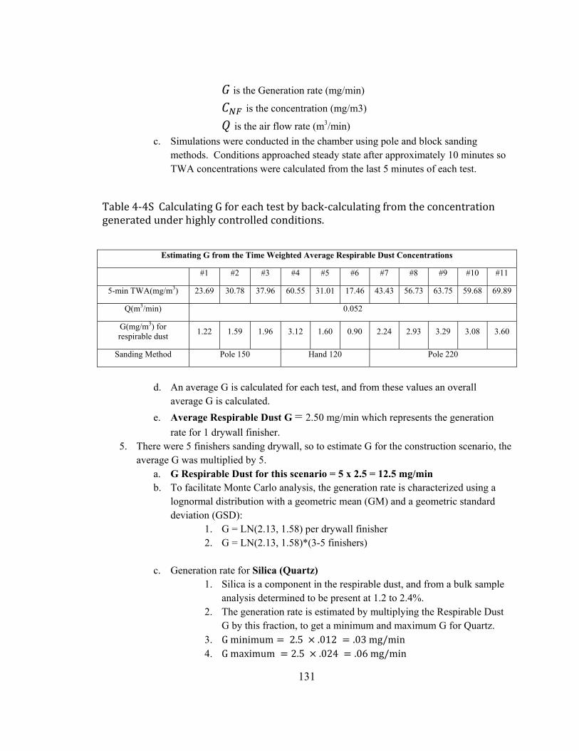
131


is the concentration (mg/m3)

is the air flow rate (m3/min)

c. Simulations were conducted in the chamber using pole and block sanding methods. Conditions approached steady state after approximately 10 minutes so TWA concentrations were calculated from the last 5 minutes of each test.

Table4‐4SCalculatingGforeachtestbyback‐calculatingfromtheconcentrationgeneratedunderhighlycontrolledconditions.

Estimating G from the Time Weighted Average Respirable Dust Concentrations

#1 #2 #3 #4 #5 #6 #7 #8 #9 #10 #11

5-min TWA(mg/m3) 23.69 30.78 37.96 60.55 31.01 17.46 43.43 56.73 63.75 59.68 69.89

Q(m3/min) 0.052

G(mg/m3) for respirable dust

1.22 1.59 1.96 3.12 1.60 0.90 2.24 2.93 3.29 3.08 3.60

Sanding Method Pole 150 Hand 120 Pole 220

d. An average G is calculated for each test, and from these values an overall

average G is calculated.

e. Average Respirable Dust G = 2.50 mg/min which represents the generation

rate for 1 drywall finisher. 5. There were 5 finishers sanding drywall, so to estimate G for the construction scenario, the

average G was multiplied by 5. a. G Respirable Dust for this scenario = 5 x 2.5 = 12.5 mg/min b. To facilitate Monte Carlo analysis, the generation rate is characterized using a

lognormal distribution with a geometric mean (GM) and a geometric standard deviation (GSD):

1. G = LN(2.13, 1.58) per drywall finisher 2. G = LN(2.13, 1.58)*(3-5 finishers)

c. Generation rate for Silica (Quartz)

1. Silica is a component in the respirable dust, and from a bulk sample analysis determined to be present at 1.2 to 2.4%.

2. The generation rate is estimated by multiplying the Respirable Dust G by this fraction, to get a minimum and maximum G for Quartz.

3. Gminimum 2.5 .012 .03mg/min 4. Gmaximum 2.5 .024 .06mg/min

132

5. For Monte Carlo analysis, G is described as a lognormal distribution: 6. LN(2.13,1.58)*U(min =0.012, max=0.24)

6. Ventilation rate (Construction environment):

a. The ventilation rate in the hospital suite was estimated, knowing that the mechanical ventilation system was turned off and covered to prevent entrainment of construction dust.

b. Q is estimated to be between 0.1 and 0.3 ACH = 1.4 to 4.3 m3/min c. For the Monte Carlo analysis, a uniform distribution was defined using these

estimates as the lower and upper bound, respectively.

7. Interzonal airflow rate: a. Local air velocity measurements were taken approximately every 3 m across the

suite at the beginning and midway through the work shift. Six 10-second samples were measured at each location, producing 88 sets of velocity measurements. The average velocity at each location was calculated and then used to calculate an overall average velocity for the suite.

b. The average local velocity, s = 5.6 m/min c. Using a hemispherical geometry with a radius of 0.8 m, the Free Surface Area

(FSA) = 2πr2 = 4.02 m2

5. 4.02 5.6 11.3

6. Room volume : (i) Calculated from measurements of each room and hallways (ii) Room volume = 860 m3

7. The Near Field Volume is calculated from the volume of a hemisphere, Where

a. Volume of a hemisphere: 2/3πr3 (i) Radius, r = 0.8 m, representing arms’ length between the operator and

the respective source. (ii) NF volume = 4.2 m3

8. The Far Field Volume is the total room volume – NF volume

a. FF volume = 860 m3 – 4.2 m3 = 875.8 m3

(6) Time: (a) This was a full shift activity. Time = 480 minutes

(7) Background respirable dust and silica:

(a) Real time measurements were used to quantify background levels in this very dusty environment, attributable to multiple days of sanding, a variety of work tasks going on concurrently, real time data. Background was quantified during the lunch break when all sanding stopped for approximately 30 minutes.

133

(b) The ambient respirable dust = 1.78 mg/m3

(c) In the model, this was accounted for by setting CIN = 1.78

Applying a Monte Carlo approach, the modeled C WMR 95th percentile exposure =8.06 mg/m3.

The ACGIH TLV for Respirable Dust (3 mg/m3) is used as the exposure benchmark. The 95th percentile respirable dust exposure, based on the real time data is 6.35 mg/m3. The reference ECC is also a Category 4.

For quartz, the 95th percentile modeled C WMR exposure based on Monte Carlo analysis = 0.16 mg/m3.

The ACGIH TLV for Quartz (0.05 mg/m3) is used as the exposure benchmark. The 95th percentile quartz exposure, based on the real time data is 0.15 mg/m3. The reference ECC is also a Category 4.

Lunch Time

134

Scenario 5. And 6. Using physical chemical models to estimate cobalt

exposure while weighing Lithium Cobalt Oxide powder, and mixing

through cleaning tasks in a clean room area.

Ingredients are weighed before being transferred to a blender for mixing. After mixing, the slurry

is transferred to another pan and moved to the staging area for the next step in the manufacturing

process. The blender and surrounding areas are cleaned using a HEPA vacuum.

Weighing was treated as a separate task and modeled separately. Mixing and cleanup tasks were

treated as one SEG for personal monitoring and modeling purposes.

1. Weighing Lithium Cobalt Oxide: a. Generation rate:

i. The Near Field acetone concentration was measured during weighing and mixing through cleaning tasks. The time weighted average

Technician weighs Lithium Cobalt Oxide powder into a pan placed on a scale

Technician adds powder to a blender to be mixed.

135

concentration used to solve for the generation rate. This relationship between C and G is:

ii. 1. Where

2. is the Generation rate (mg/min)

3. is the Near Field concentration (mg/m3)

4. is the near field ventilation rate (m3/min)

(d) A generation rate was estimated from measurements collected in the near

field on multiple occasions using a TSI DustTrak. The mean and standard deviation were calculated, and producing an overall average generation rate. On one occasion, measurements were collected directly above the source. This data was used to estimate an upper bound generation rate. The average generation rate is .044 mg/min.

Table4‐5SCalculatingtheGenerationratefromtheNearFieldConcentration,thevalueobtaineddirectlyoverthesource(G4)toestimatetheupperboundG

G1 G2 G3 G4

Concentration ppm .002 .002 .001 1.36

Q (m3/min) 3.35

G (mg/min) .007 .006 .004 4.56

Correction Factor = CTWA/CDustTrak 0.39

G (mg/min) .003 .003 .002 1.77

(e) To facilitate Monte Carlo analysis, the generation rate is characterized using

a uniform distribution. (i) G = U(minimum = .002, maximum = 1.77)

(3) Room volume :

(b) The room dimensions were measured, and the volume calculated. (i) Width = 7.9 m; Length = 5.5 m; Height = 2.9 m (ii) Volume = 7.9 x 5.5 x 2.9 = 125.9 m3



(i) Radius, r = 0.8 m, reflecting the close proximity of the salon professional to the source

136

(ii) NF volume = 1.07 m

(6) The Far Field Volume is the total room volume – NF volume (a) FF volume = 125.9 m3 – 1.07 m3 = 124.4 m3

(7) Ventilation rate:

a) Weighing and mixing tasks were conducted in a clean room area where contaminants were removed by a large slot hood. The velocity was measured at several points across the face of each of the five slots in the slot hood. The area of each slot was also measured. The distance from the scale to the hood was approximately .1 m.

Where

(i) Q (m3/min) is the ventilation rate (ii) v (m/min) is the velocity

(iii) A is the area of the slot (m2). (iv) The average ventilation rate is 3.35 m3/min

(v) For Monte Carlo Analysis, a uniform distribution was used to characterize Q. The area is a clean room area where a high degree of control over the process and environment are required, thus minimum and maximum are set ± 20% of the average Q. 1. Qminimum = 2.68 m3/min

2. Qmaximum = 4.02 m3/min

(8) Interzonal airflow rate:

(a) The interzonal airflow rate (ß) is estimated using the following formula:

i. ß

(b) where 2 . The FSA is estimated using a hemisphere to describe the near field, with a radius r = 0.8 m, reflecting the less-than arms’ length distance between the source and the salon professional.

(c) ½ free surface area = 2.01 m2 (d) where s = local air velocity and is estimated at 15 m/minute.

(e) 2.01 3.9 /min 7.8

(f) For Monte Carlo analysis, ß is characterized by a lognormal distribution. The GSD is based on the variability observed in local velocity measurements.

(g) ß = LN(7.8, 2.1)

(9) Time

137

(a) The average time to weigh the Lithium Cobalt Oxide powder was 17 minutes.

Applying a Monte Carlo approach and incorporating the upper bound estimate of G, the 95th percentile exposure for the weighing task = 0.78 mg/m3.

The measured 95th percentile exposure for the weighing task is 0.42 mg/m3, based on 7 personal exposure measurements. The OEL is 0.02 mg/m3, thus the reference ECC is Category 4.

Mixing and Cleaning:

8. Generation rate:

a. The same approach was used as for the weighing task. The Near Field acetone concentration was measured during mixing through cleaning tasks. The time weighted average concentration used to solve for the generation rate. This relationship between C and G is:

i. Where


is the Near Field concentration (mg/m3)

is the near field ventilation rate (m3/min)

(c) A generation rate was estimated from measurements collected in the near

field on multiple occasions. Cleaning tasks including vacuuming were captured on two occasions, and these values were used to characterize the distribution for G, providing minimum and maximum values for G. The average G is 4.5 mg/min.

Table4‐6SEstimatingGfromSourceSampling

G1 G2

Concentration ppm .002 .004

Q (m3/min) 3.35

G (mg/min) .08 .14

Correction Factor = CTWA/CDustTrak

0.39

G (mg/min) .03 .06

138

(d) To facilitate Monte Carlo analysis, the generation rate is characterized using a uniform distribution. (i) G = U(minimum = .03, maximum = 0.06)

(4) Room volume :

(b) The room dimensions were measured, and the volume calculated. (i) Width = 7.9 m; Length = 5.5 m; Height = 2.9 m (ii) Volume = 7.9 x 5.5 x 2.9 = 125.9 m3



(i) Radius, r = 0.8 m, reflecting the close proximity of the salon professional to the source

(ii) NF volume = 1.07 m3

(9) The Far Field Volume is the total room volume – NF volume (a) FF volume = 125.9 m3 – 1.07 m3 = 124.8 m3

(10) Ventilation rate:

The velocity was measured at several points across the face of each of the five slots in the slot hood. The area of each slot was also measured. The distance from the scale to the hood was approximately .1 m.

Where (i) Q (m3/min) is the ventilation rate (ii) v (m/min) is the velocity

(iii) A is the area of the slot (m2). (iv) The average ventilation rate is 3.35 m3/min

(v) For Monte Carlo Analysis, a uniform distribution was used to characterize Q. The area is clean room areas where a high degree of control over the process and environment are required, thus minimum and maximum are set ± 20% of the average Q. 3. Qminimum = 2.68 m3/min

4. Qmaximum = 4.02 m3/min

(10) Interzonal airflow rate:

(a) The interzonal airflow rate (ß) is estimated using the following formula:

ii. ß

139

(b) where 2 . The FSA is estimated using a hemisphere to describe the near field, with a radius r = 0.8 m, reflecting the less-than arms’ length distance between the source and the salon professional.

(c) ½ free surface area = 2.01 m2 (d) where s = local air velocity and is estimated at 15 m/minute.

(e) 2.01 3.9 /min 7.8

(f) For Monte Carlo analysis, ß is characterized by a lognormal distribution. The GSD is based on the variability observed in local velocity measurements.

(g) ß = LN(7.8, 2.1)

(11) Time (a) The average time for mixing, including cleanup is approximately 120

minutes.

Applying a Monte Carlo approach, the 95th percentile CNF exposure = .027 mg/m3.

The measured 95th percentile exposure for the mixing and cleaning tasks is 0.09 mg/m3, based on 7 personal exposure measurements. The OEL is 0.02 mg/m3, thus the reference ECC is Category 4.

140

Scenario 7. Using physical chemical models to estimate

exposure to methylene chloride:

DiagramofaColowasasampler Stainlesssteelvessel

The Near Field Far Field model is a good candidate model for this scenario, since the operator is standing

close to the vessel portal when collecting the sample.

1. Generation rate: The Colowasa sampler resembles a large ladle. Dipping the sampler through

the portal, into the vessel is analogous to drum filling, where air containing the chemical vapor is

displaced into the workplace air, and the rate of displacement is proportional to the rate at

which the sampler is lowered into the vessel. This is useful for estimating the Generation rate, G.

The following information is needed to use this approach:

a. Volumetric fill (and displacement) rate:

i. The sampler has a volumetric capacity of 460 ml. This volume of air is displaced

when the sampler is lowered into the vessel over ~ 2 minute period. The

volumetric fill rate is the volume/unit time:

1.

230

0.00023

b. Headspace (methylene chloride) concentration

i. Using the vapor pressure of methylene chloride, we can calculate the saturated

vapor concentration expected to occupy the headspace of the vessel.

141

1. VP methylene chloride = 350 mm Hg

2. Saturated vapor concentration =

10

3. Headspace concentration = saturated vapor conc’n = 460526.32 ppm

ii. Converting from ppm to mg/m3 so units are compatible with IHMOD:

1. 460525.32 . /

. / = 1.6 x 106 mg/m3

c. Generation rate:

i. Combining a and b to estimate the Generation rate, G, in mg/min:

1. / 3

2. 0.00023 1.6 10 367.93

3. The range stated in the scenario, (304 – 457 mg/min) reflects

uncertainty around the rate at which the sampler is lowered into the

vessel by the operator.

4. For Monte Carlo analysis, G is defined using a lognormal distribution,

with GM = 220 and GSD = 4.

2. Room volume

a. As stated in the scenario, = 379.4 m3


a. The general ventilation rate, calculated from the room volume and stated ACH, = 118

m3/min.

b. LEV is also used, and in the near field will contribute to the rate at which vapors are

removed. Q LEV is calculated using the ventilation rate information and area of the duct:

i. Q = VA

ii. 100 6.2 628 0.0283

17.8

c. The total ventilation rate is the sum of the general and local ventilation rates.

i. 118 17.8 136.03

ii. For Monte Carlo analysis, Q is defined using a uniform distribution, minimum =

(0.8 x 118 m3/min = 94 m3/min), maximum = (1.2 x 118 m3/min = 140 m3/min)

4. Interzonal airflow rate:

a. The interzonal airflow rate (ß is estimated using the following formula:

i. ß

1. free surface area = 1.2 m2

2. where s = local air velocity and is estimated at 3 – 6 m/minute

3. ß 3.5 7.1

4. For Monte Carlo analysis, a uniform distribution is defined using these

values the upper and lower bound estimates.

The modeled CNF 95th percentile exposure based on Monte Carlo analysis = 194.1 ppm.

142

The OEL = 125 ppm so the predicted ECC = category 4.

The reference exposure control category is category 4, with 69% probability, based on n = 10 and using the IH Data Analyzer software.

143

Scenario 8. Using physical chemical models to estimate phenol

exposure while making sand molds containing a phenolic resin

Operatorfilesroughedges Operatorfillsmold

offmold

In this scenario, the operator fills the molds with the sands/phenolic resin, which are heated in the

mold press to form the shell core. After a few minutes, he takes the shell core out and modifies its

shape, as necessary; changing the mold or repairing as necessary, by holding the shell core in one

hand, and using the other hand, files it with a hand file. This task is repeated for the entire 8 hour

shift. The 2 Zone model is a good candidate reflecting the close proximity of the operator to the

source while making the molds.

1. Interzonal airflow rate: a. The interzonal airflow rate (ß) is estimated using the following formula:

b. ß

Where i. 2

ii. The FSA is estimated using a hemisphere to describe the near field, with a radius r = 1 m, reflecting the less-than arms’ length distance between the source and the salon professional.

iii. ½ free surface area = 3.14m2 iv. where s = local air velocity and is estimated at 30 m/minute, based on

local air velocity measurements. Two fans ensure constant and relatively consistent air movement in this area.

144

v. 3.14 30 /min 94

vi. For Monte Carlo analysis, ß is characterized by a lognormal distribution. The GSD reflects the relatively moderate variability in local air velocity.

vii. ß = LN(94, 1.8)

2. Generation rate: a. An average Near Field concentration was calculated from personal TWA phenol

measurements collected over a five day period. This average was used to solve for the generation rate. This relationship between C and G is:

b. Where

i. is the Generation rate (mg/min)

ii. is the Near Field concentration (mg/m3)

iii. is the interzonal air flow rate (m3/min)

iv. From the TWA data C average = 0.196

v. = 94 m3/min

vi. Average G (mg/min) = 18.4

vii. To facilitate Monte Carlo analysis, the generation rate is characterized

using a lognormal distribution with a geometric mean (GM) and a geometric standard deviation (GSD):

viii. G = LN(13.1, 2.3)

3. Room volume : a. The shell core area is approximately 5 x 5 x 5 m (125 m3)

4. The Near Field Volume is calculated from the volume of a hemisphere,

Where a. Volume of a hemisphere: 2/3πr3 b. Radius, r = 0.8 m, reflecting the close proximity of the salon professional to the

source c. NF volume = 4.2 m

5. The Far Field Volume is the total room volume minus the NF volume

a. FF volume = 125.9 m3 – 1.07 m3 = 120.8 m3

6. Ventilation rate: a. The ventilation rate was estimated using professional judgment, informed by the

knowledge that an exterior door located next to the middle shell core machine

145

opens and closes repeatedly throughout the day. The building is in general very old and not well sealed, further promoting air movement. Based on this information, the ventilation rate is estimated to be 4 to 5 ACH.

b. 125 460 8.33

c. 125 560 10.4

d. For Monte Carlo Analysis, a uniform distribution was used to characterize Q using these estimates as the minimum and maximum values.

e. Q = U(8.33, 10.4)

7. Time a. This was a full shift activity. Time = 480 minutes.

Converting from mg/m3 to ppm, and applying a Monte Carlo approach, the modeled 95th percentile CNF exposure = 0.8 ppm.

The ACGIH TLV (5 ppm) is used as the exposure benchmark. Using the AIHA Exposure Control Categories, the predicted NF concentration falls into Category 2.

The reference exposure category is Category 2, with a 100% probability based on 8 personal samples.

146

Scenario 9. Using physical chemical models to estimate a salon

professional’s exposure to acetone in a nail salon:

Waterless manicures were given to five clients throughout the day using acetone to clean nail

surfaces. The services were offered in a new building with large, well ventilated suites in a

commercial loft setting.

The 2 Zone model is a good candidate reflecting the close proximity to which the salon professional works with acetone while giving the client a manicure.

1) Generation rate: The salon professional works across the table from the client and uses a squirt bottle to wet a cotton pad with acetone, which is then used to clean the client’s nails as part of a waterless manicure. Acetone on the nails evaporates quickly, providing a clean, dry nail surface. Some of the acetone evaporates when the cotton pad is wetted and continues to evaporate from the cotton pad until it is disposed of in a trash can and the trash can lid closed. Typically, the cotton pad is placed in the trash can as soon as this task is completed. This is the first and only source of acetone exposure unless the client chooses to have nail polish applied. When nail polish is being applied, the nails are wiped with acetone again after the bond aid, or dehydrator is applied and before the base coat is applied. For some manicures in which only buffing and shaping were done, acetone was not used and thus the generation rate for these manicures was equal to zero.

Salon Professional (right) gives client a waterless manicure using acetone to clean nails

Products used during manicure and nail painting. Acetone is used as a polish remover and non-aqueous cleaner.

147

a) The Near Field acetone concentration was measured during each manicure and used to

back-calculate, solving for the generation rate. This relationship between C and G is:

Where


is the Near Field concentration (mg/m3)

is the interzonal air flow rate (m3/min)

b) A generation rate was estimated for each manicure, from which the mean and standard deviation were calculated, producing an overall generation rate. The average generation rate was 21 mg/min.

Table4‐7SCalculatingGfromCforeachmanicure.

G1 G2 G3 G4 G5

Concentration ppm 0 0.58 0.47 0 0.10

Concentration mg/m3 1.38 1.11 0.23

Beta (m3/min) 23.10 23.10 23.10

G (mg/min) 31.98 25.75 5.25

c) To facilitate Monte Carlo analysis, the generation rate is characterized using a lognormal

distribution with a geometric mean (GM). i) G = LN(16.3, 2.68)

2) Room volume :

a) The room dimensions were measured, and the volume calculated. i) Width = 2.7 m; Length = 3.0 m; Height = 3.8 m ii) Volume = 2.7 x 3. 0 x 3.8 = 31 m3

3) The Near Field Volume is calculated from the volume of a hemisphere,

Where i) Volume of a hemisphere: 2/3πr3 ii) Radius, r = 0.7 m, reflecting the close proximity of the salon professional to the

source, (less than arm’s length) iii) NF volume = 1.03 m

4) The Far Field Volume is the total room volume minus NF volume

a) FF volume = 31 m3 – 1.03 m3 = 29.9 m3

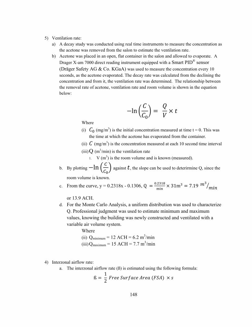
148

5) Ventilation rate: a) A decay study was conducted using real time instruments to measure the concentration as

the acetone was removed from the salon to estimate the ventilation rate. b) Acetone was placed in an open, flat container in the salon and allowed to evaporate. A

Drager X-am 7000 direct reading instrument equipped with a Smart PID® sensor (Dräger Safety AG & Co. KGaA) was used to measure the concentration every 10 seconds, as the acetone evaporated. The decay rate was calculated from the declining the concentration and from it, the ventilation rate was determined. The relationship between the removal rate of acetone, ventilation rate and room volume is shown in the equation below:

ln

Where

(i) (mg/m3) is the initial concentration measured at time t = 0. This was

the time at which the acetone has evaporated from the container.

(ii) (mg/m3) is the concentration measured at each 10 second time interval

(iii) Q (m3/min) is the ventilation rate

1. V (m3) is the room volume and is known (measured).

b. By plotting ln against , the slope can be used to deterirmine Q, since the

room volume is known.

c. From the curve, y = 0.2318x - 0.1306, Q.

31m 7.19

or 13.9 ACH. d. For the Monte Carlo Analysis, a uniform distribution was used to characterize

Q. Professional judgment was used to estimate minimum and maximum values, knowing the building was newly constructed and ventilated with a variable air volume system.

Where (ii) Qminimum = 12 ACH = 6.2 m3/min

(iii) Qmaximum = 15 ACH = 7.7 m3/min

4) Interzonal airflow rate:

a. The interzonal airflow rate (ß) is estimated using the following formula:

ß 1

2

149

Where

(i) 2 . The FSA is estimated using a hemisphere to describe the near field, with a radius r = 0.7 m, reflecting the less-than arms’ length distance between the source and the salon professional.

(ii) ½ free surface area = 1.54 m2 (iii) where s = local air velocity and is estimated at 15 m/minute.

(iv) 1.54 15 /min 23.1

b. For Monte Carlo analysis, ß is characterized by a lognormal distribution. The GSD is based on professional judgment and represents low variability.

c. ß = LN(23.1, 1.1) 5) Time

a. While the time varied from client to client depending on the service provided, the average time for a manicure was 35 minutes.

From the Monte Carlo approach, the 95th percentile exposure = 11.9 ppm for a single manicure. A time weighted average concentration is calculated assuming each manicure lasts 35 minutes, there are five manicures and there are no other exposures to acetone for the remaining work shift.

5 11.9 35

4804.33

.

The ACGIH TLV (8 hour TWA = 250 ppm) is used as the exposure benchmark. Using the AIHA Exposure Control Categories, the predicted NF concentration falls into Category 1.

The measured TWA 95th percentile exposure to acetone = 9.75 ppm. The reference exposure category is Category 1, with a 100% probability based on 10 personal samples.

150

Scenario 10. Using physical chemical models to estimate

acetone exposure while cleaning the lid and blades of a

Morehouse mixer

Technicianscleaningslurrypotlidandblades,alternatelysquirtingthesurfaceswithacetoneandwipingthemoffwithpaperwipes

The slurry pot lid and blades are cleaned by alternately applying acetone, from a squirt bottle and wiping the blades and lid with a paper wipe. Some of the acetone evaporates immediately; some falls or drips from the blades into the slurry pot and the remainder is wiped off using the paper wipes, which are then deposited in an uncovered trash can. The 2 Zone model is a good candidate given the close proximity of the technician to the source while cleaning the mixer.

1. Generation rate: a. The Near Field acetone concentration was measured while the lid and blades

were cleaned and the time weighted average concentration used to solve for the generation rate. This relationship between C and G is:

i. Where

151

ii. is the Generation rate (mg/min)

iii. is the Near Field concentration (mg/m3)

iv. is the interzonal air flow rate (m3/min)

b. Near Field concentration measurements were made on several days, from which the mean and standard deviation were calculated, producing an overall generation rate.

Table4‐8SBackcalculatingfromCtoestimateG.Theaveragegenerationratewas1638.2mg/min.

G1 G2 G3 G4

Concentration ppm

62.7 127.8 96.8 72.7

Concentration mg/m3

149.3 289.9 229.8 173.1

Beta (m3/min) 7.8

G (mg/min) 1161.7 2367.4 1788.0 1346.7

c. To facilitate Monte Carlo analysis, the generation rate is characterized using a lognormal distribution with a geometric mean (GM).

d. G = LN(1600, 1.37)

2. Room volume : a. The room dimensions were measured, and the volume calculated. b. Width = 7.9 m; Length = 5.5 m; Height = 2.9 m c. Volume = 7.9 x 5.5 x 2.9 = 125.9 m3

3. The Near Field Volume is calculated from the volume of a hemisphere, Where a. Volume of a hemisphere: 2/3πr3 b. Radius, r = 0.8 m, reflecting the close proximity of the salon professional to the

source c. NF volume = 1.07 m

4. The Far Field Volume is the total room volume – NF volume

a. FF volume = 125.9 m3 – 1.07 m3 = 124.8 m3


a. A Drager X-am 7000 direct reading instrument equipped with a Smart PID® sensor (Dräger Safety AG & Co. KGaA) was used to measure the concentration every 10 seconds, as the acetone evaporated after all cleaning tasks were finished. The decay rate was calculated from the declining the

152

concentration and from it, the ventilation rate was determined. The relationship between the removal rate of acetone, ventilation rate and room volume is shown in the equation below:

ln

Where

(mg/m3) is the initial concentration measured at time t = 0. This was the time at which the

acetone has evaporated from the container.

(mg/m3) is the concentration measured at each 10 second time interval

Q (m3/min) is the ventilation rate

V (m3) is the room volume and is known (measured).

By plotting ln against , the slope can be used to deterirmine Q, since the room

volume is known.

From the curve, y = 0.1025x + 1.194, .

126m 12.8 or 6.2 ACH.

For Monte Carlo Analysis, a uniform distribution was used to characterize Q. The area is a clean room area where a high degree of control over the process and environment are required, thus minimum and maximum values corresponding to 5 and 7 ACH respectively represent a conservative estimate of the expected variability in the system. Qminimum = 10.1 m3/min

Qmaximum = 15.1 m3/min Interzonal airflow rate:

The interzonal airflow rate (ß) is estimated using the following formula:

ß 1

2

where 2 . The FSA is estimated using a hemisphere to describe the near field, with a radius r = 0.8 m, reflecting the less-than arms’ length distance between the source and the salon professional.

½ free surface area = 2.01 m2

where s = local air velocity and is estimated at 15 m/minute.

153

2.01 15 /min 15.6

For Monte Carlo analysis, ß is characterized by a lognormal distribution. The GSD is based on professional judgment and represents low variability.

ß = LN(15, 1.1)

Time

The average time to clean the lid and blades was 20 minutes.

Applying a Monte Carlo approach, the 95th percentile modeled CNF exposure = 439 ppm.

The ACGIH TLV (STEL = 500 ppm) is used as the exposure benchmark. Using the AIHA Exposure Control Categories, the predicted NF concentration falls into Category 3.

The reference exposure category is Category 3, with a 100% probability based on 6 personal samples.

154

CHAPTER5 CONCLUSIONSANDFUTUREDIRECTION

OVERALLCONCLUSIONS Exposure judgments are used in a wide range of situations, including retrospective

exposure assessments for epidemiology studies (e.g. Esmen, 1979; Ramachandran 2001;

Ramachandran et al., 2003; Friesen, 2003) and current as well as prospective exposure

assessments for managing exposures related to consumer use and manufacturing

operations (e.g. Hawkins and Evans 1989; Teschke et al. 1989; Macaluso et al., 1993;

Friesen et al., 2003; Ramachandran et al., 2003; Jones et al., 2014). When there are

limited or no sampling data available, hygienists use a combination of professional

judgment, personal experience with a given operation, and review of exposures from

similar operations to assess the acceptability of exposures for managing engineering

controls, medical surveillance, hazard communication and personal protective equipment

programs (Teschke et al., 1989; de Cock et al., 1996; Burstyn & Teschke, 1999; Friesen,

2003; Kolstad, et al., 2005; Logan et al., 2009; Logan, et al., 2011; Vadali et al., 2012a;

Vadali et al., 2012b). In many cases, there is not an opportunity to collect quantitative

measurements prior to making an exposure assessment judgment. For example, hazard

communications triggered by an exposure assessment must be made prior to the

introduction of the agent into the workplaces similarly; a theoretical technical basis is

often the only thing available to define adequate engineering controls related to the

introduction of new processes or changes in existing processes. The term “qualitative”

refers to judgments or decisions made in the absence of quantitative personal exposure

data. This term can be further subdivided according to the type of inputs from which the

155

judgments are synthesized; subjective qualitative judgments are based on intuition or

‘personal experience’ that is derived from unstructured inputs and is not overtly defined.

Objective qualitative judgments are produced using structured, more transparent

approaches.

Research has shown that subjective, unstructured qualitative exposure judgments tend to

be no more accurate than random chance, with a significant underestimation bias, i.e.,

there is marked tendency to assign a lower exposure category than the correct one, thus

increasing occupational risk to workers (Logan et al. 2009; Vadali et al., 2012; Arnold et

al., 2015). The low accuracy could be due to several factors. OHs receive little, if any

formal training on how to conduct a basic characterization. If this step of the exposure

assessment is not conducted in a systematic way, using physical and chemical principles,

and collecting the relevant exposure determinant information, the hygienist may not

investigate the exposure that presents the highest exposure potential with sufficient detail,

leading to low judgment accuracy. Another factor may be cognitive biases in

understanding skewed lognormal distributions (Logan, 2009). Mental shortcuts, known as

heuristics, are often used, making the decision process efficient but can lead to errors in

judgment and introduce bias. Using these heuristics leads to a pattern that, when faced

with uncertain prospects, assigns weights to our decisions that differ from the true

probabilities of these outcomes. Improbable outcomes are over-weighted, while almost-

certain outcomes are under-weighted.

Objective, structured approaches, using simple algorithms and exposure modeling are

more resistant to these vulnerabilities, focusing the decision maker on the decision

156

making process, and on the critical inputs, while filtering out nonessential information.

These approaches have been shown to improve decision making across a broad range of

domains, including psychology (Kahneman, 2011 and Kahneman et al.,, 1982), drug

delivery and development (Lipinski, et al., 2001); predicting transdermal delivery and

toxicity (Magnusson et al., 2004;) environmental exposure assessment ( Fristachi, et al.,

2009); and aggregate exposure assessment (Cowan-Ellsberry & Robison, 2009). These

same objective approaches can be applied to occupational exposure assessment. In fact,

decisions are most accurate in highly uncertain ‘low validity’ environments, i.e. situations

with little or no data, when the final decision is generated from algorithms.

One of the characteristics of algorithms and models contributing to consistent decision

making is the consistent order in which information is processed. Checklists provide

guidance on the order in which inputs are considered. These simple tools have been the

cornerstone of safety excellence in the aviation industry for years. To be sure, checklists

and models do not replace knowledge and expertise, and pilots go through rigorous

training before they are allowed to fly. The checklists ensure they follow the critical

steps at the right time to ensure theirs, and their passengers’, safety. Likewise, checklists

help hygienists focus on the critical inputs to decision making in the right order, leading

to consistent and accurate exposure judgments (Arnold et al., 2015), protecting the health

and safety of those in their care.

Exposure models seek to capture the underlying physical processes generating chemical

concentrations in the workplace. An accurate representation will produce better

concentration estimates and facilitate decision-making in exposure management.

157

However, this is challenging because workplaces are notoriously complex and no

physical model is likely to provide a complete representation. Thus, characterizing model

parameters, and accounting for parameter and model uncertainty is crucial. Guidance on

selecting and applying the models appropriately is also essential. Without these,

hygienists may select the wrong model or use model input values that are inappropriate

and misleading. Further, without guidance on how to interpret the model output relative

to making decisions about the acceptability of an exposure, the hygienist may draw

conclusions that are not consistent with the ‘true’ magnitude of exposure.

This research was conducted to evaluate the use of several structured, objective

approaches, namely the use of checklists and heuristics and exposure models in

improving qualitative exposure judgment accuracy. Three major studies were

investigated to meet this objective, with each study generating a manuscript. Chapter 2

discusses the development and application of a foolproof checklist for using heuristics

and algorithms. It has already been accepted for publication (JOEH, 2015). Chapter 3 and

4 discuss evaluation of the Well Mixed Room (WMR) and Near Field Far Field (NF FF)

models, conducted in a way that is analogous to the way in which a NIOSH method is

validated, identifying the bounds within which the models are useful, as well as their

limitations. Specifically, Chapter 3 discusses model evaluation under highly controlled

conditions, in which model parameters are known and well controlled, providing near-

ideal model conditions. In Chapter 4, model evaluation under less controlled conditions,

using scenarios from real workplaces is discussed. The impact of selecting the wrong

158

model is also discussed in Chapter 4. Chapters 3 and 4 will be submitted to the Annals of

Occupational Hygiene in the near future.

The primary conclusions of these papers are:

1. Previously published research suggested that when hygienists make decisions

regarding the acceptability of exposure based on professional judgment guided by

unstructured, subjective inputs, their exposure judgment accuracy is low, and not

statistically significantly different from random chance. Moreover, the data

indicated a negative bias in these decisions, resulting in a tendency to

underestimate exposures, with a consequent risk of inadequately managing

unacceptable exposures and risks.

A study was conducted in which a database of exposure scenarios were

developed, capturing reasonably well defined model input values and including a

minimum dataset of six personal exposure measurements. The personal exposure

data was used to characterize the reference exposure control category (ECC),

representing the ‘true’ exposure and against which qualitative exposure judgment

accuracy was measured. A new tool, the Qualitative Exposure Assessment

Checklist was constructed for this research, comprised of heuristics and

algorithms that were developed from physical and chemical principles but refined

empirically, over many years. These heuristics were presented in a structured

format; a checklist requiring only a few inputs that guided the hygienist through

the selection, application and interpretation of the results. Using this tool,

exposure judgment accuracy was evaluated by collecting exposure judgments

159

from novice and practicing hygienists that were made with and without guidance

from the tool.

2. Exposure judgment accuracy of exposure judgments made by practicing

hygienists without the benefit of personal exposure measurement data and based

on professional judgment guided by subjective inputs were ~ 30% accurate, no

better than random chance and tended to underestimate the true exposure. These

results were consistent with the study results reported by previous investigators

(Logan et al., 2009; Logan et al., 2011; Vadali, et al. 2011; Vadali et al., 2012).

Exposure judgment accuracy made by novice hygienists in the absence of

personal exposure data was slightly higher than those of their more experienced

colleagues but not statistically significantly different from random chance.

However, the novices’ judgments did not exhibit the same negative bias; they

were equally balanced between over and underestimating the true exposure. When

exposure judgments were guided by the Checklist, a statistically significant

increase in judgment accuracy was observed with both practicing and novice

hygienists. In fact, exposure judgment accuracy increased by a factor of 2 to ~

65% and was highly statistically significant (p <0.001). Moreover, the negative

bias observed in judgments made by practicing hygienists was reduced. Thus the

main conclusions of this research is that exposure judgments made in the absence

of robust personal exposure measurement data, but based on professional

judgment that is guided by structured, objective inputs are likely to be more

accurate than random chance and significantly more accurate than judgments

160

guided by unstructured, subjective inputs. The checklist format for applying the

heuristics is essential to improving exposure judgment accuracy as it ensures the

heuristics are applied in consistently and appropriately and that the output is

interpreted correctly. Exposure models, such as the Well Mixed Room (WMR)

and Near Field Far Field (NF FF) models have been found to be useful for

estimating exposures to chemicals across a range of situations. The literature is

scattered (Esman et al., 1999; Ramachandran 2001; Ramachandran et al., 2003; Friesen,

2003, Hawkins and Evans 1989; Teschke et al. 1989; Macaluso 1993) anecdotal case

study reports indicating these models are useful for predicting exposures in

retrospective epidemiological studies to facilitate dose reconstruction, for guiding

product stewardship recommendations for best work practices aimed at

minimizing exposure, when it is not feasible to collect a robust dataset of personal

exposure measurements and in prospective exposure studies to guide scale up

from pilot to manufacturing activities. However, models tend to be undervalued

and underutilized by hygienists. Several factors may influence this trend,

including a lack of model selection and application guidance and the scarcity of

model input values needed to use the models. Another possible reason they have

not been more readily adopted in practice is that their performance relative to

accurately predicting exposure had not been systematically evaluated.

A study was conducted to test whether these models works well under controlled

conditions where the models’ underlying assumptions are met. These tests were

conducted in an exposure chamber in which three chemicals were used to evaluate

161

model performance of the WMR and NF FF models across a range of conditions.

The chamber allowed conditions to be controlled so that they could be changed

one at a time and measured with a reasonable degree of confidence. This

generated high quality model inputs and measured contaminant concentration data

and consequently produced over 800 modeled and measured exposure pairs,

against which model performance was measured. Two sets of criteria, the ASTM

Standard 5157, providing insight regarding general concordance across the time-

varying spectrum of exposures and identifying potential for systematic bias, and

the AIHA Exposure Assessment categorical criteria providing insight the model’s

ability to predict the TWA exposure and thus predict the correct ECC.

Model performance of the WMR model across all three chemicals and chamber

conditions was excellent, with ≥ 82% of the 483 of Cmeasured-Cmodeled pairs deemed

adequate, meeting all ASTM performance criteria. Categorically, the WMR

model predicted the correct ECC for 93% of the 27 scenarios. In comparing

categorical accuracy of the WMR model to accuracy attributable to random

chance alone, the WMR model accuracy was highly statistically significant (p <

0.001). Model performance for the NF FF model was impacted by the physical

limitations of the chamber in generating a true NF FF environment, so model

performance of the NF modeled exposures relative to the ASTM 5157

performance criteria was low, with only 11 to 33% of the Cmeasured and Cmodeled NF

pairs deemed adequate. Categorically, and more relevant to their use to hygienists,

model performance was much higher and highly statistically significant (p

162

<0.001), with the model predicting the correct ECC for 20/27 NF scenarios

(~74%). Model performance of the FF modeled exposures stronger than the NF

based on the ASTM 5157 performance criteria, with 163 of the 243 Cmeasured and

Cmodeled FF pairs deemed adequate (~ 67 %) and categorically, producing excellent

concordance, with 26/27 FF scenarios (~96%) predicting the correct ECC. These

results, relative to model accuracy based on random chance alone were highly

statistically significant (p <0.001).

There are several important implications of this study:

1. The models are designed to provide a reasonable estimation of the average

concentration in a room, and when environmental conditions parallel the

underlying assumptions of the model, model performance of both models is

strong. Moreover, when the contaminant concentration is generated by a source

whose behavior parallels the assumptions of the model in its relevant form, e.g.,

time-varying, model performance is excellent.

2. The AIHA categorical criterion is a better performance metric that the very strict

ASTM 5157 for models that will be used to assess occupational exposures.

3. Characterizing the generation rate with a reasonable degree of certainty was

instrumental in achieving the observed performance levels.

Model performance under field (work place) conditions may differ from performance

evaluated under highly controlled conditions. Two types of uncertainty will come into

163

play in such studies; (1) parameter uncertainty, when we do not know the parameter

values under these field conditions precisely, and (2) model uncertainty, when it is not

abundantly clear which model should be used. Selecting the best candidate model likely

is an important component of generating accurate estimates of the exposure, but the

choice is not always obvious and selecting the wrong model can result in categorical ly

misclassifying the exposure. For all these reasons, it is important to understand model

performance under real work place conditions.

A study was conducted under these less than ideal conditions to evaluate model

performance by evaluating ten scenarios from a diverse range of workplaces and tasks,

involving four chemical agents. Personal exposure measurements were collected

following a similar protocol to the approach used in the chamber study and were used to

define the reference ECC for each scenario. Model input values were measured directly

whenever possible, and estimated using submodels or professional judgment guided by

input from site hygienists and work area experts. Time varying measurements, necessary

for applying the ASTM 5157 criteria were collected for six of the scenarios. Categorical

performance criteria were applied to all ten scenarios, based on the 95th percentile

measured and modeled exposures.

Model performance based on the ASTM criteria was low, with none of the six scenarios

achieving scores within the defined ranges for all parameters using the WMR or NF FF

models. Categorically, however, performance was excellent, with the WMR model

predicting the correct ECC in 8/10 scenarios, and the NF FF model predicting the correct

164

ECC in 9/10 scenarios. Model performance accuracy for both models, relative to random

chance was both highly statistically significant (p < 0.001).

Implications of this research are three-fold:

1. Model performance was heavily influenced by the ability to generate reasonably

high quality generation rates. The efforts invested were not trivial but are valuable

beyond the specific scenarios for which they were developed. These generation

rates will be useful in assessing other scenarios involving the same agent under

similar conditions, thus the generation rates have portability.

2. Categorical model performance was highly statistically significant, even when

model performance as defined by ASTM Standard 5157 was poor. Thus, this

standard, with its strict criteria is not recommended for evaluating performance of

models intended to be used to guide decisions regarding the acceptability of

occupational exposure.

3. Selection and application of the models also required a significant intellectual

investment and required judicious professional judgment. Thus a checklist is

needed to provide guidance for the systematic selection and application of the

models.

Limitations of the Study and Future Directions

This research produced several novel tools, evidence to support the use of models in

guiding exposure judgments, especially when personal exposure data are not available or

insufficient. A data base of model input values was generated under highly controlled

165

(chamber) conditions and less controlled, (field) conditions that was previously were not

available. Several practical field methods for characterizing model inputs were applied

that were found to produce reasonably accurate estimates. Future research, expanding on

this foundation could include:

Chamber Studies:

1. Expanding the chamber study conditions to further explore the bounds in which

the models are useful to hygienists

2. Evaluating different types of exposure scenarios, including exposures resulting

from the use of consumer products

3. Expanding the chamber studies to evaluate the impact of aerosols on model

performance

4. Evaluating additional models, such as the turbulent eddy diffusion model

Field Studies:

1. Developing a checklist to guide hygienists in selecting and applying the models

and interpreting model output appropriately and consistently.

2. Developing a library of generation rates for standard industrial tasks, e.g. sanding,

cutting, drum filling of solvents, etc.

Model Application Studies

1. Validating the modeling checklist, demonstrating that hygienists can select and

apply the best model candidate and interpret the model output appropriately when

guided by the checklist.

166

2. In conjunction with validating the modeling checklist, a database of exposure

scenarios needs to be developed to support model checklist validation workshops.

167

BIBLIOGRAPHY ACGIH. (1995). Industrial Ventilation: A Manual of Recommended Practice. Cincinatti: ACGIH.

Apgar, V., Holaday, D., James, L., Weisbrot, I., & Berrien, C. (1958). Evaluation of the newborn

infant ‐ second report. JAMA, 168(15) 1985‐1988.

Arnold, S., Ramachandran, G., & Jayjock, M. (2009). Model Selection. In Mathematical Models

for Estimating Occupational Exposure to Chemicals, 2nd Edition. Fairfax: AIHA Press.

Arnold, S., Stenzel, M., & Ramachandran, G. (2015). Approaches to Improving Professional

Judgment Accuracy. In S. Jahn, J. Ignacio, & W. Bullock, A Strategy for Assessing and

Managing Occupational Exposures (pp. 90‐ 110). Fairfax: AIHA Press.

Arnold, S., Stenzel, M., Drolet, D., & Ramachandran, G. (2015). Using Checklists and Algorithms

to Improve Qualitative Exposure Judgment Accuracy. JOEH.

Ashenfelter, O. (2008). Predicting the quality and prices of bordeaux wine. The Economic

Journal, 118 (529) F174 ‐ F184.

ASTM. (2014). Standard Guide for Statistical Evaluation of Indoor Air Quality. West

Conshohocken: ASTM International.

Billings, C., & Reynard, W. (1984). Human factors in aircraft incidents: results of a 7‐year study.

Aviat Space Environ Med, 55 (10) 960 ‐ 965.

Brennan, R. (1992). Generalizabiliy Theory. An Instruction Module. New York: Springer‐Verlag.

Burstyn, I., & Teschke, K. (1999). Studying the Determinants of Exposure: A Review of Methods.

AIHA J, 60:57‐72.

Cherrie, J. (1999). The effect of room size and general ventilation on relationship between near

and far field concentration. App Occup and Env Hygiene J, 14, 539‐546.

Cohen, J. (1960). A coefficient of agreement for nominal scales. Psychological Measurement, Vol

20 (1) 37‐46.

Cowan‐Ellsberry, C. E., & Robinson, S. H. (2009). Refining Aggregate Exposure: Example using

Parabens. Regulatory Toxicology and Pharmacology, 321‐329.

de Cock, J., Kromhout, H., Heederik, D., & Burema, J. (1996). Experts' subjective assessment of

pesticide exposure in fruit growing. Scand J Work Environ Health, 22:425‐32.

168

Earnest, C., & Corsi, R. L. (2013). Inhalation Exposure to Cleaning Products: Application of a Two‐

Zone Model. JOEH, 10:6 328‐335.

Esman, N., Hall, T., Stone, R., Marsh, G., Gula, M., & Gause, C. (1999). An Investigation of

Secondary Exposure Missclassification Effects of Lifelong Occupational History in

Exposure Estimation. AIHA J, 60:175‐181.

Fleiss, J. (1971). Measuring nominal scale agreement among many raters. Psychological Bulletin,

Vol 76 (5) 378 ‐ 382.

Friesen, M., Demers, P., Spinelli, J., & Le, N. (2003). Validation of a Semi‐Quantitative Job

Exposure Matrix at Soderberg Aluminum Smelter. Ann of Occup Hygiene, 47 477‐484.

Fristachi, A., Xu, Y., Rice, G., Impellitteri, C. A., Carlson‐Lynch, H., & Little, J. C. (2009). Using

Probabilistic Modeling to Evaluate Human Exposure to Organotin in Drinking Water

Transported by Polyvinyl Chloride Pipe. Risk Analysis, 1615‐1628.

Gawande, A. (2010). The Checklist Manifesto: How to Get Things Right. New York: Metropolitan

Books.

Glaser, R., & Chi, M. T. (1988). Overview. In M. T. Chi, R. Glaser, & M. J. Farr, The Nature of

Expertise. Hillsdale: Lawrence Erlbaum Associates, Inc.

Hallgreen, K. (2012). Computing Inter‐Rater Reliability for Observational Data: An Overview and

Tutorial. Tuto Quant Methods Psychol, 8 (1) 23‐24.

Hanzawa, H., Melikow, A., & Fanger, P. (1987). Airflow Characteristics in the Occupied Zone of

Ventilated Spaces. ASHRAE transactions, 524‐539.

Hawkins, N. C., & Evans, J. S. (1989). Subjective estimation of toluene exposures: a calibration

study of industrial hygienists. App Ind Hyg J, 4 61‐68.

Hemeon, W. (1963). Plant and Process Ventilation, 2nd Edition. New York: Industrial Press.

Hewett, P., Logan, P., Mulhausen, J., Ramachandran, G., & Banerjee, S. (2006). Rating Exposure

Control Using Bayesian Decision Analysis. Journal of Occupational and Environmental

Hygiene, 3:10 568 ‐ 581.

Ignacio, J., & Bullock, B. (2006). A Strategy for Assessing and Managing Occupational Exposures,

3rd Edition. Fairfax: AIHA Press.

Jones, R. (2008). Experimental evaluation of a Markov model of contaminant transport in indoor

environments with applicaiton to tuberculosis transmission in commercial passenger

aircraft. Berkely: University of California.

169

Jones, R. M., Simmons, C., & Boelter, F. (2011). Development and Evaluation of a Semi‐Empirical

Two‐Zone Dust Exposure Model for a Dusty Construction Trade. JOEH, 8:337‐348.

Kahneman, D. (2011). Thinking, Fast and Slow. Straus and Giroux.

Kahneman, D., Slovic, P., & Tversky, A. (1982). Judgment under uncertainty: Heuristics and

biases. Cambridge: Cambridge University Press.

Keil, C., & Murphy, R. (2006). An Application of Expsoure Modeling in Exposure Assessments for a

University Chemistry Teaching Laboratory. JOEH.

Keil, C., Simmons, C., & Anthony, T. (2009). Mathematical Models for Estimating Occupational

Exposures to Chemicals, 2nd Edition. Fairfax: AIHA Press.

Kolstad, H. A., Sonderskov, J., & Burstyn, I. (2005). Company‐Level, Semi‐Quantitiative

Assessment of Occupational Styrene Exposure when Individual Data are not Available.

Ann. occup Hyg., 155‐165.

Kromhout, H., Oostendorp, Y., Heederik, D., & Boleij, J. (1987). Agreement between qualitative

exposure estimates and quantitative exposure measurements. Am. J. Ind. Med., 2:551‐

562.

Landis, J., & Koch, G. (1977). The measurement of observer agreement for categorical data.

Biometrics, 33 (1) 159‐174.

Lipinski, C., Lombardo, F., Dominy, B., & Feeney, P. (2001). Experimental and computational

approaches to estimate solubility and permeabiliyt in drug delivery and development

settings. Adv. Drug Del. Rev., 46:3‐26.

Logan, P. R., & Hewett, P. (2009). Occupational Exposure Decisions: Can Limited Data

Interpretation Training Help Improve Accuracy? Am. Occup. Hyg., 1‐14.

Logan, P., Ramachandran, G., & Mulhausen, J. (2011). Desktop Study of Occupational Exposure

Judgments: Do Education and Experience Influence Accuracy. JOEH, 746‐758.

Luby, S., Agboatwalla, M., Feiken, D., Painter, J., Billhimer, W., Altaf, A., & Hoekstra, R. (2005).

Effects of handwashing on child health: a randomized control trial. The Lancet, Vol 366

(9481) 225 ‐ 233.

Magnusson, B. M., Pugh, W. J., & Robers, M. S. (2004). Simple Rules Defining the Potential of

Compounds for Transdermal Delivery or Toxicity. Pharmaceutical Research, 1047‐1054.

Malacuso, M. (1993). Inter‐rater agreement in the assessment of solvent exposure at a car

assembly plant. American Industrial Hygiene Association Journal, 54 351‐359.

170

Meehl, P. (1954). Clinical Versus Statistical Prediction: A Theoretical Analysis and a Review of the

Evidence. Minneapolis: University of Minnesota Press.

Mulhausen, J., & Damiano, J. (1998). A Strategy for Assessing and Managing Occupational

Exposures, 2nd Edition. Fairfax: AIHA Press.

Nicas, M. (1996). Estimating exposure intensity in an imperfectly mixed room. American

Industrial Hygiene Association Journal, 18 200‐210.

Pronovost, P., Needham, D., Berenholtz, S., Sinopoli, D., Chu, H., Cosgrove, S., . . . Goeschel, C.

(2006). An Intervention to Decrease Catheter‐Related Bloodstream Infections in the ICU.

N. Engl J Med, 355 2725 ‐ 2732.

Putka, D., McCloy, R., & Diaz, T. (2008). Ill‐Structured Measurement Designs in Organizational

Research: Implications for Estimating Interrater Reliability. Journal of Applied

Psychology, Vol. 91 (5) 959 ‐ 981.

Ramachandran, G. (2001). Retrospective Exposure Assessment using Bayesian Methods. Ann

Occup Hyg, 45(8) 651‐667.

Ramachandran, G. (2005). Occupational Exposure Assessment of Air Contaminants. CRC.

Ramachandran, G. (2008). Toward Better Exposure Assessment Strategies ‐ The New NIOSH

Initiative. Annals of Occupational Hygiene, 52, 297‐301.

Ramachandran, G., & Banerjee, S. (2003). Expert Judgment and Occupational Hygiene:

Application to Aerosol Speciation in the Nickel Primary Production Industry. Ann Occup.

Hyg, 47(6) 461 ‐ 475.

Stenzel, M., & Arnold, S. (2015). Rules and Guidelines to Facilitate Professional Judgment. In S.

Jahn, J. Ignacio, & W. Bullock, A Strategy for Assessing and Managing Occupational

Exposures (pp. 150 ‐ 160). Fairfax: AIHA.

Taylor, J., & Watkins, D. (2007). Indexing Reliability for Condition Survey Data. The Conservator,

Vol. 30 49 ‐ 61.

Teschke, K., Hertzman, C., Dimich‐Ward, H., Ostry, A., Blair, J., & Hershler, R. (1989a). A

comparison of exposure estimates by worker raters and industrial hygienists. Scand J

Work Environ Health, 15:424‐429.

Vadali, M., Ramachandran, G., & Banerjee, S. (2011). Effect of Training, Education, Professional

Experience and Need for Cognition on Accuracy of Exposure Assessment Decision‐

Making. Ann Occup Hyg, 56(3) 292‐304.

171

Vadali, M., Ramachandran, G., Mulhausen, J., & Banerjee, S. (2012). Effect of Training on

Exposure Judgment Accuracy of Industrial Hygienists. JOEH, 242‐256.

172

APPENDIX I

Figure5‐1BayesianDecisionChart,showingtheIHsbeliefthatthe95thpercentileoftheexposuredistributionforagivenscenariomostlikelybelongstoExposureControlCategory(ECC)4.

1%

9%

30%

60%

0%

20%

40%

60%

80%

100%

1 2 3 4

Exposure Control Category

Pro

babi

lity

of

the

95th

per

cent

ile

bein

g lo

cate

d in

an

expo

sure

con

trol

cat

egor

y

173

Figure5‐2CategoricalJudgmentAccuracy,showingaccuracyattributabletorandomchancepre‐training(Baseline),post‐trainingChecklist‐guidedjudgmentaccuracyforNovicesandpracticingIHs.

0%

20%

40%

60%

80%

100%

‐3 ‐2 ‐1 Accurate +1 +2 +3

Per

cent

Acc

urac

y

Categorical AccuracyRandom ChanceNovice baselineNovice ChecklistPracticing IH baseline

174

Figure5‐3BaselineandChecklistbasedjudgmentaccuracyforNoviceIHs

and practicing IHs respectively, broken out by scenario

0%

20%

40%

60%

80%

100%

1 2 3 4 5 6 7 8 9 10 11

Percent Accuracy

Scenario

Random chance Novice IH Baseline Novice IH Checklist

Practicing IH Baseline Practicing IH Checklist

175

Table5‐1AIHAExposureControlCategories(ECC)withcriteriaforinterpretation

Exposure Control Category (ECC)

Criteria for Statistical Interpretation

1 X0.95 ≤ 0.1 × OEL

2 0.1 × OEL < X0.95 ≤ 0.5 × OEL

3 0.5 × OEL < X0.95 ≤ OEL

4 X0.95 > OEL

176

Table5‐2Ruleof10EngineeringControlMatrix

Level of Control Fraction of the Saturation Vapor Concentration (SVC)

Confined Space – Virtually no circulation

1/10th of Saturation

Poor – Limited Circulation 1/100th of Saturation

Good – General ~ 6 Air Changes/Hour 1/1,000th of Saturation

Capture 1/10,000th of Saturation

Containment 1/100,000th of Saturation

177

Table5‐3VaporHazardRatio(VHR)EngineeringControlMatrix

Vapor Hazard Ratio (VHR)

VHR

Scale

Required Level of Control

(ReqLC)

< 0.05 1 General Ventilation

~ 3 to 6 air changes /hr.

0.05 to < 1 2 Good general ventilation

~ 6 to 12 air changes/hr. (GGV)

1 to < 25 3 GGV with capture at emission points

25 to < 500 4 Capture at points of emission with containment wherever practical

500 to < 3000 5 Containment

> 3000 6 Primary and Secondary Containment

178

Table5‐4ParticulateHazardRatio(PHR)EngineeringControlMatrix

OEL Range

(mg/m3)

PHR Scale Required Level of Control

(ReqLC)

5 1 General ventilation

~ 2 to 4 air changes/hr.

≤ 5 to 1 2 Good – General + fans


≤ 1 to 0.1 3 Good – General + fans


≤ 0.1 to 0.01 4 Capture

≤ 0.01 to 0.001 5 Containment

≤ 0.001 6 Secondary containment

179

Table5‐5TheChecklist‐anorderedapproachtoapplyingthethreeheuristics

Rule of 10 1. Select the appropriate Occupational Exposure Limit (OEL)

2. Determine the Vapor Pressure & Saturated Vapor Concentration (SVC)

3. Identify the Observed Or Reported Level of Control (ObsLC)

4. Estimate the fraction of the SVC

5. Calculate the maximum concentration ( Cmax)

6. Compare the Cmax to the OEL

7. Determine the predicted Exposure Control Category (ECC)

Vapor Hazard Ratio (VHR) 1. Divide VP/OEL to determine VHR Score 2. Identify Required Level of Control (ReqLC) from VHR matrix 3. Compare ReqLC with ObsLC 4. Determine ECC: If ObsLC > ReqLC= 1

If ObsLC = ReqLC = 2 If ObsLC < ReqLC = 4

5. If the ECC’s based on Rule of 10 & VHR differ, use the highest ECC

Particulate Hazard Ratio

(PHR)

1. Identify OEL 2. Identify ReqLC from PHR matrix 3. Compare ReqLC with ObsLC 4. Determine ECC: If ObsLC > ReqLC = 1

If ObsLC = ReqLC = 2 If ObsLC < ReqLC = 4

Table5‐6ExposureScenarioDetails,showingtheScenarionumber,agentofconcern(ChemicalAgent),therelevantOEL,theprimarytaskorworkprocessfrom

180

whichtheexposureoccurred(Process),thenumberofpersonalexposuresamplescollected,fromwhichtheReferenceECCwascalculated(ReferenceECCdataset)andthecorrespondingReferenceECC.

Scenario Chemical Agent OEL Process Number of measureme

nts in Reference ECC data set

(n)

ECC

1 Glutaraldehyde Cal OSHA ceiling: 0.05 ppm

Neutralizing, dumping and pouring liquid

6 2

2 Mannitol NIOSH REL: 8 hour TWA: 0.25 μg/m3

Potent compound transfer

6 2

3 Trichloro‐ethylene

ACGIH TLV TWA: 5 ppm

Spray cleaning degreaser

11 4

4 Asbestos OSHA PEL: 8 hour TWA: 0.1 f/cc

Locomotive steamline repair

9 2

5 Isopropanol OSHA PEL: 8 hour TWA 400 ppm

Cleaning printing presses

8 2

6 Hexavalent chromium

OSHA PEL: 8 hr. TWA: 0.5 mg/m3

Repair – welding railroad frog

8 4

7 Asbestos OSHA PEL: 30 min. excursion limit: 1

f/cc

Bystander exposure in locomotive repair

shop

29 1

8 Acetone OSHA PEL: 8 hour TWA: 1000 ppm

Cleaning printing presses

8 1

9 Phenol ACGIH TLV: TWA: 5 ppm

Foundry shell core – mold making

8 1

10 Quartz ACGIH TLV TWA for α‐quartz = 0.025

mg/m3

Foundry shake out – breaking molded

parts

8 4

11 Methylene chloride

OSHA PEL: 15 min. STEL: 125 ppm

Collecting a sample from a vessel

10 4

181

Table5‐7aResultsfromnoviceIHs’exposurejudgments,showingbias(thedifferencebetweentheaveragepredictedECCandreferenceECC),andPrecision(standarddeviation)foreachscenario(n=8)

Scenario Bias Precision Baseline Checklist Baseline Checklist

1 0.5 -.13 0.84 0.98 2 0.3 -.25 0.64 0.46 3 -0.5 0 0.76 0 4 -3 0 0 0 5 0.3 0.8 0.64 1.04 6 -1 0 0 0 7 0.5 1.6 0.84 0.92 8 1.3 1.3 1.2 1.16 9 -1 0 1.19 0 10 -1 -1.6 1.19 1.06

182

Table2‐7bResultsfrompracticingIHexposurejudgments,showingbias,(thedifferencebetweentheaveragepredictedECCandreferenceECC),andPrecision(standarddeviation)foreachscenarioby.

Scenario n Bias Precision Baseline

Checklist Baseline Checklist Baseline Checklist

1 2 10 0 -0.7 NA 0.48 2 3 10 1 -0.6 1.00 0.52 3 30 29 -1.1 -0.1 0.94 0.33 4 2 10 -0.5 -0.3 0.71 .95 5 7 9 -0.7 0.3 0.57 0.87 6 4 11 -1.5 -0.5 1.0 1.00 7 4 3 1.2 1.2 0.5 1.17 8 6 6 1.5 1.7 1.0 1.32 9 2 9 0 0 0 0 10 2 9 -2 1.4 NA 1.01

Table5‐8ExposureScenariousingtheOELasthebenchmark,OEL=10ppm,GSD=2.5

EF GM 95th % (ppm)

Distribution < AL

Probability (%) that All Indicated Measurements of Dataset Size N (N = 1,2,3, 4 or 5) Will Fall

Below the OEL

N = 1 N = 2 N = 3 N = 4 N = 5

0.5 10 45.15 0.5 50 25 12.5 6.25 3.13

0.25 5.39 24.32 0.75 75 56.3 42.2 31.6 23.7

0.1 3.09 13.95 0.9 90 81 72.9 65.6 59.1

0.05 2.22 10 0.95 95 90.3 85.7 81.5 77.4

0.02 1.52 6.87 0.98 98 96 94.1 92.2 90.4

183

APPENDIX II Well Mixed Room Model

The Well Mixed Room (WMR) model considers exposures as a factor of air movement

into, through and out of a room and the generation rate of a contaminant within the room.

A key assumption of this model is that air in the room is completely and instantaneously

well mixed; a physically unrealistic but useful construct for estimating the average

concentration when the contaminant is generated from a large or non-point source.

(Ramachandran, 2005)

While there are various forms of the model depending on the contaminant source, the

constant emission source will be described here since it is the form used in this study.

Several terms are invoked to apply the conservation of mass principle, accounting for the

movement of contaminant mass. . In a room of volume, V (e.g. m3) with a constant

ventilation rate, Q (m3/min), air entering the room has a contaminant concentration of Cin

(mg/m3), and a contaminant source in the room, C (mg/m3) generating an airborne

concentration at a constant generation rate, G (mg/min). Thus, as air enters the room and

the source contributes contaminant to the room air the contaminant concentration in the

room increases.

Air enters and exits the room, either actively, via mechanical ventilation systems or

passively, through doors and windows or cracks and spaces around them. We assume that

the rate at which air enters is the same as when air exists the room, i.e., Qin = Qout and

thus drop the subscripts.

When air leaves the room, it removes some of the contaminant. Contaminant mass may

also be removed by other mechanisms, for example, vapor and gases may adsorb onto

184

surfaces in the room and aerosols of certain size ranges may be lost due to gravitational

settling. These loss mechanisms are summed up into one loss term, denoted by kL. Thus,

the contaminant concentration in the room is reduced as these mechanisms remove the

contaminants from the room air.

The general equation for the WMR model as a function of time is expressed as:

1

0

(A-1)

At steady state, the expression compresses to

(A-2)

Near Field Far Field Model

When a person is located close to a contaminant source, the WMR model will

underestimate that person’s exposure. The Near Field Far Field (NF FF) model is

designed to account for this deficiency, but at a cost of added complexity, and the non-

trivial investment in acquiring data to characterize the additional model inputs.

This model assumes a two box construct, with the air within each box well mixed. The

area close to and around the source is the Near Field (NF) and can be described using a

range of geometries, such as a box, sphere, hemisphere, etc. The geometry is defined

on a scenario by scenario basis. The rest of the room is the Far Field (FF).

The supply and exhaust flow rates are the same, and denoted by Q (m3/min),

consistent with the WMR model. Air movement from one box to the other is called the

interzonal airflow rate and is denoted by the symbol ß (m3/min). Q can be measured

185

directly in many cases, but quantifying ß is more complicated. The most common

approach to estimate ß is to determine the product of the random air speed at the NF

FF boundary and one half the free surface area (FSA) of the NF.(Ramachandran,

2005). Thus, ß is somewhat dependent on the geometry used to define the NF.

(A-3)

The ½ accounts for the fact that as ß flows into the NF through one half the FSA, ß

flows out of the NF through the other half of the FSA.

The NF and FF equations are

exp

exp (A-4)

exp

exp (A-5)

Where 0.5

4 (A-6)

And 0.5

4 (A-7)

186

At Steady State, these equations shrink considerably to:

(A-8)

(A-9)

the use of heuristics and exposure models in improving

Documents