the use of fuzzy spaces in signal detection final draft
TRANSCRIPT
The Use of Fuzzy Spaces in Signal Detection
S. W. Leung and James W. Minett
Department of Electronic Engineering, City University of Hong Kong
Correspondence to:
Dr. Peter S. W. Leung
Department of Electronic Engineering
City University of Hong Kong
Tat Chee Avenue
Kowloon Tong
Kowloon
Hong Kong

2
The Use of Fuzzy Spaces in Signal Detection
S. W. Leung and James W. Minett
Abstract: The Fuzzy CFAR (Constant False Alarm Rate) detector, which is based on the M-
out-of-N binary detector, is characterized and compared with the optimal Neyman-Pearson
detector. It replaces the crisp M-out-of-N binary threshold with a soft, continuous threshold,
implemented as a membership function. This function is chosen so that the output is equal to
the false alarm rate of the binary detector, and therefore maps the observation set to a False
Alarm Space corresponding to the false alarm rate, PFA. An analogous membership function
is also developed mapping observations to a Detection Space which corresponds to the
detection rate, PD. These two spaces allow different detectors to be compared directly with
respect to the two important detection performance indices, PFA and PD. Comparison of the
False Alarm Space and Detection Space indicates that the Fuzzy CFAR detector and
Neyman-Pearson detector detect signals in a different manner and have different detection
properties. Nevertheless, performance results illustrate that the Fuzzy CFAR detector
achieves detection performance comparable to the optimal Neyman-Pearson detector.
Keywords: Decision Making; Signal Detection
1. Introduction
Constant False Alarm Rate (CFAR) detectors [4, 8-10] and other threshold-based detectors
[7, 12] form the basis of many decision making systems such as in radar detection and digital
communication. Detection algorithms are generally optimized with respect to a particular set
of cost functions chosen for the specific application. In this paper we present the Fuzzy
3
CFAR detector [5-6] and compare it to the Neyman-Pearson detector [1, 12-13], which
provides optimal detection in many situations in which cost is too vague for meaningful
assignment of cost functions [13]. We describe the underlying principles and detection
criteria for each detector, and also show how the Fuzzy CFAR detector is adapted from the
classic M-out-of-N binary detector [10]. We go on to discuss the use of Fuzzy Spaces [6],
explaining how they allow analysis and direct comparison of the detection properties of
detectors.
2. Detection Criteria
In signal detection, we are often interested in determining the presence of a weak signal,
corrupted by noise. CFAR detectors generally implement decision rules based on a crisp
threshold producing binary output, either 0 or 1 [10]. Often, such discontinuous decision
rules give rise to a significant loss of information, producing far from optimal detection
performance. The Fuzzy CFAR detector replaces the binary threshold with a soft, continuous
threshold producing smooth output in order to reduce information loss. The following
sections compare the detection criteria of this detector with the optimal Neyman-Pearson
detector, and the classic M-out-of-N detector which it adapts.
Noise can be modeled as a random process, reducing the detection problem to a statistical
hypothesis test. An appropriate hypothesis test for detection of a signal in a noisy channel is
"":"":
1
0
TargetnMyHTargetNonyH
+==
, (2.1)
where y represents an observation of the channel, n the observed noise, and M the signal
which may be present in the channel. In this study, we consider only the basic case of a
constant signal in zero-mean white Gaussian noise, with observations assumed independent
and, therefore, uncorrelated [1]. Although simple, this model allows us to introduce the
4
concepts required to characterize the Fuzzy CFAR detector, and to compare it to the
Neyman-Pearson and M-out-of-N detectors. We now present a brief review of each detector,
including the derivation of the Fuzzy CFAR detector from the M-out-of-N detector.
2.1 Neyman-Pearson Criterion
The Neyman-Pearson criterion specifies the optimal decision rule for a hypothesis test with
constrained rate of false alarm and is often used when the cost functions associated with
hypotheses are unknown. The Neyman-Pearson detector is implemented as shown in Figure
1. For each observation set, N independent measurements of the detection channel are made.
The mean value is then thresholded to provide the target decision.
For our chosen noise/signal model with N independent observations, the Neyman-Pearson
threshold, THX, is given implicitly by [1]
( ), ∑
=
=≥=N
iiX
FA YN
XHTHXP1
01
:Pr:, (2.2)
where PFA is the chosen false alarm rate; hypothesis “Target” is accepted when X ≥ THX .
This produces the Neyman-Pearson decision rule
( )FAX
Target
PN
THX −Φ=<≥ − 1: 1σ
Target No
, (2.3)
where Φ-1 is the inverse cumulative distribution function of the standard Gaussian
distribution, and σ2 is the noise mean power. The detection rate is given by [1]
( )1Pr: HTHXP XD ≥= , (2.4)
which for Gaussian noise is
( )
−−ΦΦ−= −
σ11 11 MNPP FAD , (2.5)
where Φ is the cumulative distribution function of the standard Gaussian distribution.

5
2.2 M−out−of−N Criterion
The M-out-of-N or Binary detector found widespread application in the early years of radar
when operators were still using head-phones to listen to the detection channel [10]. Although
now little used as a detector, it forms the basis for the new class of fuzzy detectors introduced
by the authors in [5-6]. The M-out-of-N detector is shown in Figure 2 as used for radar
detection. At each range bin, N observations are made, as for the Neyman-Pearson detector.
However, each observation, yi, is thresholded independently, producing binary output, µ(yi),
≥<
NYi
NYi
iTHyTHy
y:1:0
: aµ . (2.6)
These binary outputs are then summed and a “Target” is declared when the sum is greater
than or equal to M, i.e.
( ) My
TargetN
ii
Target No<≥
∑=1
µ . (2.7)
The threshold, THYN, is defined implicitly by
( ){ }∏=
≥=Mj
ji
NYi
FA HTHYP1
0Pr: , (2.8)
or equivalently
( )
MjjiN
YiM FA YYYHTHYP ,,allforPr:
10 …=≥=, (2.9)
reflecting the fact that at least M of the N observations should exceed the chosen threshold
with constrained false alarm rate.
The detection rate is given by
( ){ }∏=
≥=Mj
ji
NYi
D HTHYP1
1Pr , (2.10)
which for Gaussian noise is

6
( ) NN FAD MPP
−−ΦΦ−= −
σ11 11 . (2.11)
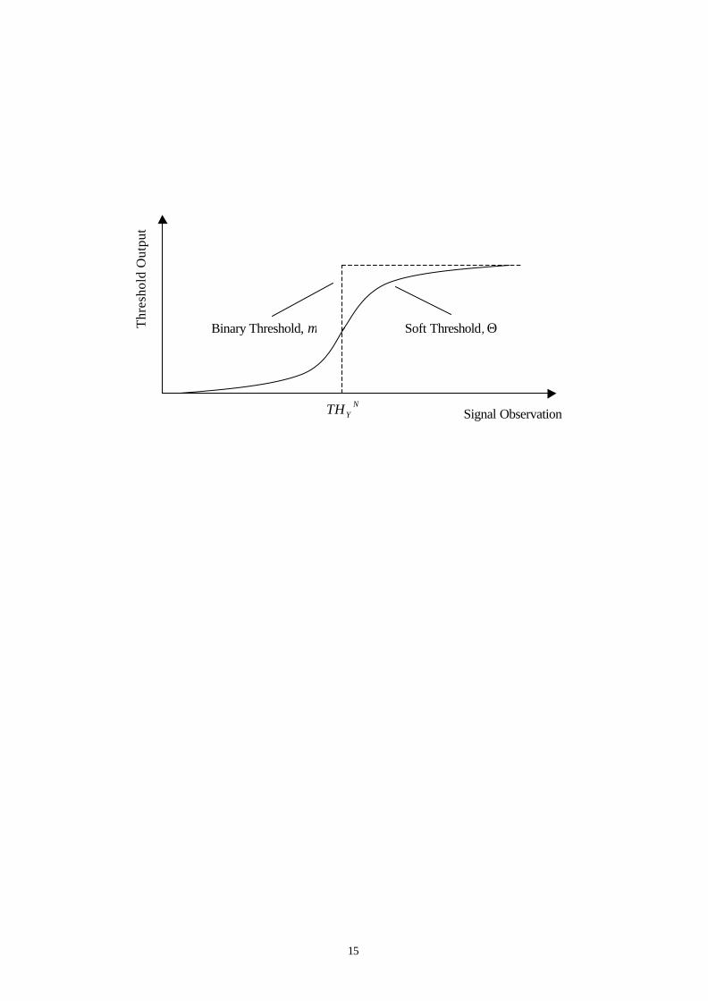
2.3 Fuzzy Criterion
The Fuzzy CFAR detector adapts the M-out-of-N detector by replacing the binary threshold
of Equation 2.6 with a soft threshold, shown in Figure 3. The reason for adapting the M-out-
of-N detector in this way is to deal with the uncertainty in selecting a fixed value of the
binary threshold, THYN; this new fuzzy threshold provides soft decisions with a smooth
transition from certain acceptance to certain rejection of a hypothesis. In this way the
detector retains more information than the binary detector.
The soft threshold is implemented as a fuzzy membership function [3, 14], Θ (yi), assigning
membership to hypothesis H0, “No Target”. Furthermore, it is defined so that membership
values are distributed uniformly on [0,1] under H0,
( )0~Pr: Hyy ii ζζ ≥Θ a , (2.12)
so that Θ(yi) is the probability that an observation exceeds threshold yi under the “No Target”
hypothesis. The reason for this particular definition is two-fold:
• The membership function is monotone decreasing, guaranteeing that stronger
observations are assigned smaller membership to the “No Target” hypothesis,
i.e. ( ) ( )jiji yyyy Θ≤Θ⇔≥ ; (2.13)
• The M-out-of-N criterion, as interpreted in equation (2.9), requires that the false alarm
rate associated with at least M individual observations be smaller than some threshold for
a “Target” to be declared. With our choice of membership function, the M-out-of-N
decision rule can be written as
( )Mjji
M FA
Target
i yyyPy ,,1
…=∀≥<
ΘTarget No
, (2.14)

7
hence presenting the threshold explicitly in terms of false alarm rate.
The Fuzzy CFAR criterion adapts this decision rule by declaring “Target” when the false
alarm rate associated with the entire observation set is small enough. Since observations are
independent, the Fuzzy CFAR decision rule for N observations is given by
( ) FA
etNoT
TargetN
ii Py
arg1 ≥
<Θ∏
=
, (2.15)
where threshold, PFA, is just the false alarm rate of the associated M-out-of-N detector,
allowing the False Alarm Space concept to be developed in Section 3. The block diagram of
the Fuzzy CFAR detector is shown in Figure 4. With this detector, if even a single
observation suggests “Target” with sufficient certainty (Θ(yi) << 1), the detector outputs
“Target.” This will be discussed further in Section 3.2.
In our simple example, the membership function is
Φ−Θ σ
yy 1: a , (2.16)
the complement of the cumulative distribution function under H0, and has the form shown in
Figure 3. The false alarm rate of the N scan detector is
( ) ( )∑−
=
−=1
1 !ln
1N
i
iiFA
N iP
αα , (2.17)
while the detection rate is given by the integral
( )
∫∏
=
=Θ
N
i iy
ND
N dydyP
1
1
α
… . (2.18)
3. Fuzzy Spaces
A standard method for comparing the performance of detectors is to consider the detection
rate achieved at chosen false alarm rates. It may often be instructive to consider which
observations give rise to the differences in the quoted detection and false alarm rates. In this

8
section, we look into this by defining two new spaces, the False Alarm Space and the
Detection Space, which make the comparison of such differences trivial.
3.1 False Alarm Space
The “No Target” membership function, Θ, defined in equation (2.12) maps the observation
space, S := ℜN, into a fuzzy hyper-cube [4], ℑN := [0,1]N. The threshold of each detector
forms an N – 1 dimensional subspace of ℑN, partitioning it into a False Alarm Region, ℑ1,
and a Rejection Region, ℑ0. Under H0, observations which map to a point in ℑ1 result in an
incorrect acceptance of H1, i.e. a false alarm. Observations which map to a point in ℑ0 result
in a correct rejection of H1. Due to the choice of membership function, Θ, and the
independence of observations, the false alarm rate of a detector is simply the hyper-volume of
its associated False Alarm Region, ℑ1 [6]. We therefore call ℑN the False Alarm Space.
Figure 5 shows the threshold and False Alarm Region for each detector projected into the
False Alarm Space. In order to clearly illustrate the form of each threshold, we show the
False Alarm Space at 10% false alarm rate in two dimensions only. However, the thresholds
have the same general form at higher dimensions. The False Alarm Regions differ
considerably, highlighting how different observations generate false alarms for each detector:
• The Neyman-Pearson detector favors selecting the “Target” hypothesis, H1 when Θ(yi) for
both observations is sufficiently small – the False Alarm Region has non-linear bound;
• The M-out-of-N binary detector with 2-out-of-2 decision rule selects H1, whenever Θ(yi)
for both observations is smaller than the threshold, and with 1-out-of-2 decision rule
selects H1 whenever Θ(yi) for either observation is smaller than the threshold
FAFA PP =1
– the False Alarm Region is bounded by a square;
9
• The Fuzzy CFAR detector favors selecting H1 when Θ(yi) for either observation is
sufficiently small – the False Alarm Region is bounded by a hyperbola.
It is these differences in the False Alarm Regions of each detector that give rise to differences
in detection performance, discussed in the following section.
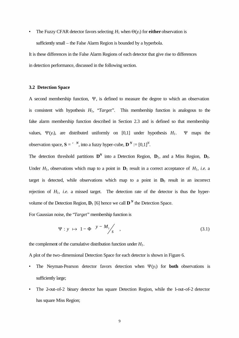
3.2 Detection Space
A second membership function, Ψ, is defined to measure the degree to which an observation
is consistent with hypothesis H1, “Target”. This membership function is analogous to the
false alarm membership function described in Section 2.3 and is defined so that membership
values, Ψ(yi), are distributed uniformly on [0,1] under hypothesis H1. Ψ maps the
observation space, S = ℜN, into a fuzzy hyper-cube, ∆ N := [0,1]N.
The detection threshold partitions ∆N into a Detection Region, ∆1, and a Miss Region, ∆0.
Under H1, observations which map to a point in ∆1 result in a correct acceptance of H1, i.e. a
target is detected, while observations which map to a point in ∆0 result in an incorrect
rejection of H1, i.e. a missed target. The detection rate of the detector is thus the hyper-
volume of the Detection Region, ∆1 [6] hence we call ∆ N the Detection Space.
For Gaussian noise, the “Target” membership function is
−Φ−Ψ σ
11: Myy a , (3.1)
the complement of the cumulative distribution function under H1.
A plot of the two-dimensional Detection Space for each detector is shown in Figure 6.
• The Neyman-Pearson detector favors detection when Ψ(yi) for both observations is
sufficiently large;
• The 2-out-of-2 binary detector has square Detection Region, while the 1-out-of-2 detector
has square Miss Region;

10
• The Fuzzy CFAR detector favors detection when Ψ(yi) for either observation is
sufficiently large.
Without calculating the actual detection rates of the detectors, it is apparent that the Fuzzy
CFAR detector generates fewer detections than the Neyman-Pearson detector when
observations are approximately equal (region D1–), but more detections when observations
are significantly different (region D1+). For a general N scan, the Neyman-Pearson detector
selects “Target” when all observations are sufficiently large, whereas the Fuzzy CFAR
detectors also allows the “Target” hypothesis to be selected when even a single observation is
sufficiently large.
These differences in the Detection Regions of the Neyman-Pearson and Fuzzy Detectors may
be significant in certain applications, such as in radar detection of Swerling 2 & 4 fluctuating
targets [11] when signal observations may vary more rapidly than expected.
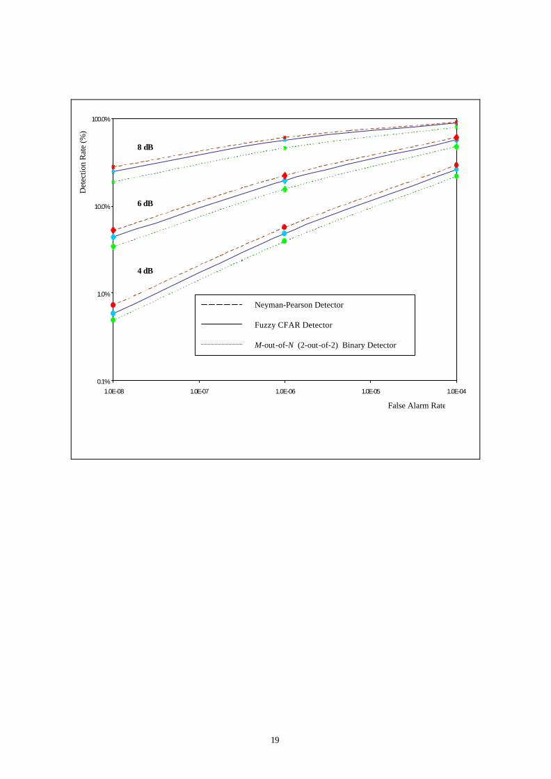
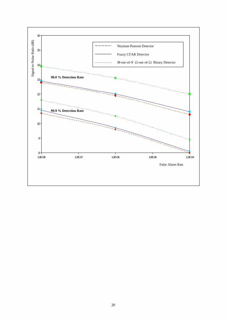
4. Performance
The performance characteristics of each detector are summarized in Figures 7 & 8. Figure 7
plots the detection rate for each detector at several practical false alarm rates, while Figure 8
shows the signal-to-noise ratio (SNR) required for each detector to achieve the specified
detection performance.
The M-out-of-N detector provides poorer detection performance than either the Neyman-
Pearson detector or the Fuzzy CFAR detector, due mainly to its use of a binary threshold. It
is also evident that for a two scan scheme, the performance of the Fuzzy CFAR detector
differs by no more than 0.2 dB from that of the optimal Neyman-Pearson detector. As
discussed in Section 3.2, the Fuzzy CFAR detector may also be less susceptible to
degradation of detection performance when, due to uncertain knowledge of target
fluctuations, signal observations fluctuate more rapidly than expected.
11
5. Conclusion
This paper has reviewed the principles of signal detection using both binary and fuzzy
thresholds to implement decision rules. The Fuzzy CFAR detector has been shown to out-
perform the classic M-out-of-N binary detector, which it extends, and to have performance
comparable to that of the optimal Neyman-Pearson detector. By particular choice of the
threshold membership function, the threshold of the Fuzzy CFAR detector is related directly
to the false alarm rate.
A method for analyzing the performance of a detector by projecting its threshold into two
fuzzy spaces, the False Alarm Space and the Detection Space, has been demonstrated. The
false alarm rate and detection rate of the detector can be calculated from the hyper-volume of
the False Alarm Region and Detection Region, respectively. Moreover, detectors can be
characterized and compared in terms of these spaces by examining which observations give
rise to false alarms and valid detections.
References
[1] M. H. DeGroot, Probability and Statistics, 2nd. Ed., (Addison-Wesley, Reading MA,
1989) 437-452.
[2] H. M. Finn & R. S. Johnson, Adaptive Detection Mode with Threshold Control as a
Function of Spatially Sampled Clutter-Level Estimates, in: RCA Review 29 (1968) 414-
464.
[3] G. J. Klir and T. A. Folger, Fuzzy Sets, Uncertainty and Information, (Prentice Hall,
Englewood Cliffs, 1992) 1-32.
[4] B. Kosko, Neural Networks and Fuzzy Systems, (Prentice Hall, Englewood Cliffs, 1992)
262-295.
12
[5] S.W. Leung, Signal Detection by Fuzzy Logic, in: Proc. of FUZZ-IEEE/IFES ‘95,
Yokohama, Japan (Mar. 20-24, 1995) 199-202.
[6] S.W. Leung and James W. Minett, Signal Detection Using Fuzzy Membership
Functions, in: Proc. SYS’95 International AMSE Conference, Brno, Czech Rep. (July 3-
5, 1995) pp. 89-92 .
[7] J. Minkoff, Signals, Noise & Active Sensors - Radar, Sonar, Laser Radar, (John Wiley &
Sons, New York, 1992) 87-96 .
[8] D. T. Nagle and J. Saniie, Performance Analysis of Linearly Combined Order Statistic
CFAR Detectors, in: IEEE Trans. Aerospace & Electronic Systems 31 (1995) 522-533.
[9] Raghavan, Qiu and McLaughlin, CFAR Detection In Clutter With Unknown Correlation
Properties, in: IEEE Trans. Aerospace & Electronic Systems 31 (1995) 647-656.
[10] M. Skolnik, Radar Handbook, 2nd Ed., (McGraw-Hill, New York, 1990).
[11] R. Swerling, Probability of Detection for Fluctuating Targets, in: IRE Trans. IT-6 (April,
1960) 269-308.
[12] H. L. Van Trees, Detection, Estimation and Modulation Theory, Vol. 1, (John Wiley &
Sons, New York, 1968) 19-4.
[13] P. K. Varshney, Distributed Detection and Data Fusion, (Springer-Verlag, New York,
1997).
[14] L.A. Zadeh, Fuzzy Sets, in: Information & Control, Vol. 8, (1965) 338-353.
13
Figure 1 Block diagram of the Neyman-Pearson Detector
Average Scans
Square LawDetector
W Bins
NScans per Bin
Target Decisionfor each Bin
Bin
Average
Threshold each BinNeyman-Pearson
Threshold
Choose FalseAlarm Rate
TestBins
1 W
14
Square LawDetector
threshold each bin to producebinary output
sum binary output
Target Decisionfor each Bin
W Bins
Nscans per bin
TestBin
M-out-of-Nthreshold
Choose FalseAlarm Rate
compare summed output with M
TestBin
15
Binary Threshold, µ Soft Threshold, Θ
Signal Observation N
YTH
Thr
esho
ld O
utpu
t

16
Square LawDetector
apply membership functionto each bin
Multiply Scans
MembershipFunction
Target Decisionfor each Bin
BinProduct
threshold each binFuzzy CFAR
Threshold
Choose FalseAlarm Rate
W Bins
NScans per Bin
TestBins
1 W

17
Membership, Θ (y1) 1.0
Mem
bers
hip,
Θ (y
2)
0.0
1.0
Neyman-Pearson Threshold
Fuzzy CFAR Threshold
0.0
M-out-of-N Threshold
18
Membership, Ψ (y1) 1.0
Mem
bers
hip,
Ψ (y
2)
0.0
1.0
0.0
D1+
D1+
D1-
Neyman-Pearson Threshold
Fuzzy CFAR Threshold
M-out-of-N Threshold
19
0.1%
1.0%
10.0%
100.0%
1.0E-08 1.0E-07 1.0E-06 1.0E-05 1.0E-04
Neyman-Pearson Detector
Fuzzy CFAR Detector
M-out-of-N (2-out-of-2) Binary Detector
8 dB
6 dB
4 dB
False Alarm Rate
Det
ectio
n R
ate
(%)
20
8
9
10
11
12
13
14
15
16
1.0E-08 1.0E-07 1.0E-06 1.0E-05 1.0E-04
99.9 % Detection Rate
Neyman-Pearson Detector
Fuzzy CFAR Detector
M-out-of-N (2-out-of-2) Binary Detector
90.0 % Detection Rate Sign
al-to
-Noi
se R
atio
(dB
)
False Alarm Rate

21
Figure Captions
Figure 1. Block Diagram of the Neyman-Pearson Detector
Figure 2. Block Diagram of the M-out-of-N Binary Detector
Figure3. Comparison of Binary and Soft Threshold
Figure 4. Block Diagram of the Fuzzy CFAR Detector
Figure 5. Threshold and False Alarm Region of the Fuzzy CFAR, Neyman-Pearson and M-out-of-N Detector.
(Signal-to-Noise Ratio = 0 dB, False Alarm Rate = 10%)
Figure 6. Threshold and Detection Region of the Fuzzy CFAR, Neyman-Pearson and M-out-of-N Detector.
(Signal-to-Noise Ratio = 0 dB, False Alarm Rate = 10%)
Figure 7. Plot of Detection Rate against False Alarm Rate
(Signal-to-Noise Ratio 4 dB, 6 dB, and 8 dB)
Figure 8. Signal-to-Noise Ratio against False Alarm Rate
(Detection Rate 90.0 % and 99.9 %)