the use of actual or forecast depreciation in energy ...€¦ · the use of actual or forecast...
TRANSCRIPT
999
The use of actual or forecast depreciation in energy network regulation
Report prepared for Australian Energy Market Commission
31 May 2012
Denis Lawrence and John Kain
Economic Insights Pty Ltd 6 Kurundi Place, Hawker, ACT 2614, AUSTRALIA Ph +61 2 6278 3628 Fax +61 2 6278 5358 Email [email protected] WEB www.economicinsights.com.au ABN 52 060 723 631
Actual vs Forecast Depreciation
CONTENTS
Executive Summary ...............................................................................................................ii
1 Introduction....................................................................................................................1
2 Building Blocks Regulation and the NER .....................................................................2
2.1 Building blocks regulation and the opening RAB.................................................2
2.2 Relevant provisions of the NER ............................................................................3
2.3 The AER’s rule change proposal for depreciation in the roll–forward .................5
3 Theoretical Incentive Effects .........................................................................................7
3.1 General incentive considerations ...........................................................................7
3.2 Financial capital maintenance and depreciation–related incentives......................9
4. Quantifying the Incentive Effects ................................................................................14
4.1 Incentive power results using modified AER model ...........................................14
4.2 Incentive power modelling results presented in submissions..............................22
5 Recent Regulatory Practice and Experience................................................................24
5.1 Australian Energy Regulator ...............................................................................24
5.2 IPART..................................................................................................................26
5.3 Essential Services Commission ...........................................................................27
5.4 Victorian Minister’s Appeal ................................................................................28
5.5 United Kingdom...................................................................................................29
5.6 United States ........................................................................................................32
5.7 New Zealand ........................................................................................................32
5.8 Summary ..............................................................................................................33
6 Stakeholders’ Views ....................................................................................................34
7 Conclusions..................................................................................................................39
References............................................................................................................................44
i
Actual vs Forecast Depreciation
EXECUTIVE SUMMARY
Background
The AEMC has asked Economic Insights to provide advice on the incentive effects of using actual versus forecast depreciation when rolling forward the regulatory asset base from the start of the current regulatory period to the start of the next regulatory period. This topic forms part of the capex incentive arrangements component of the rule changes proposed by the AER relating to the economic regulation of electricity network services.
The AER rule change proposes to require the regulator to specify the use of either actual or forecast depreciation for the RAB roll–forward for transmission NSPs so that the treatment of transmission in the rules becomes consistent with that of distribution. Currently the rules require the use of actual depreciation in the RAB roll–forward for transmission.
In this report we review the incentive effects of using actual and forecast depreciation in rolling forward the RAB. We then quantify the incentive power of the two options using a modified version of the AER (2012a) model, examine recent regulatory practice across a range of jurisdictions and consider guidelines for the exercise of the regulator’s discretion.
Incentive effects
The use of actual depreciation can generally be expected to provide higher powered incentives for constraining capex growth. This arises because if the NSP underspends its forecast capex during a regulatory period, it keeps the benefit of the higher forecast depreciation allowance within period while also having a smaller write–down of the opening RAB for the next regulatory period than would be the case if the RAB roll–forward was done on the basis of the higher forecast depreciation (where the forecast was set at the start of the preceding regulatory period). The NSP is then able to obtain a return on a higher RAB in subsequent regulatory periods than would be the case had forecast depreciation been used.
Conversely, if the NSP overspends its capex forecast then it has a lower depreciation allowance within the regulatory period than its actual depreciation and also has its rolled–forward RAB for the start of the next regulatory period written–down more when actual depreciation is used in the roll–forward than when the original forecast depreciation is used.
As a result, the use of actual depreciation in the roll–forward provides more incentive for the NSP to underspend its forecast capex and/or to contain the size of any overspend than does the use of forecast capex, all else equal.
However, higher powered incentives associated with using actual depreciation have to be offset against a number of potential distortionary effects. These include an incentive for NSPs to overinflate their capex forecasts at the start of the regulatory period. Since the NSP will obtain a benefit from underspending its forecast capex if actual depreciation is subsequently used as the basis of the RAB roll–forward, it will be in the NSP’s interests to exploit its information asymmetry and persuade the regulator that its capex requirements for the coming period will be higher than they really are. This would lead to consumers paying more than they need to. Conversely, if the originally forecast depreciation is used in the roll–forward then the NSP has an incentive, compared to using actual depreciation, to ensure its capex forecasts at the start of the period are relatively accurate so that the asset stays on the
ii
Actual vs Forecast Depreciation
regulatory accounts for a similar period of time as on its statutory accounts (which should ideally be similar to the asset’s physical life).
Another potential source of distortion arising from the use of actual depreciation relates to the incentive powers afforded assets with different lengths of life. The use of actual depreciation leads to NSPs retaining a higher share of the benefits from underspending capex on assets with shorter lifetimes (eg information technology) compared to those with longer lifetimes (eg poles and wires). This arises because capex will generally be a higher proportion of RAB for short life assets compared to long life assets – as asset life shortens, spending on the asset becomes more akin to being fully expensed and a higher proportion of the RAB will have to be spent each year to simply maintain the size of the RAB. This means that underspending on a very short life asset compared to a very long life asset will lead to a relatively larger increase in the rolled forward RAB if actual depreciation is used in the roll–forward compared to if forecast depreciation is used. There is hence an incentive to concentrate capex reductions on the shortest life assets and, conversely, not to increase capex on short life assets, all else equal.
Quantifying the incentive effects
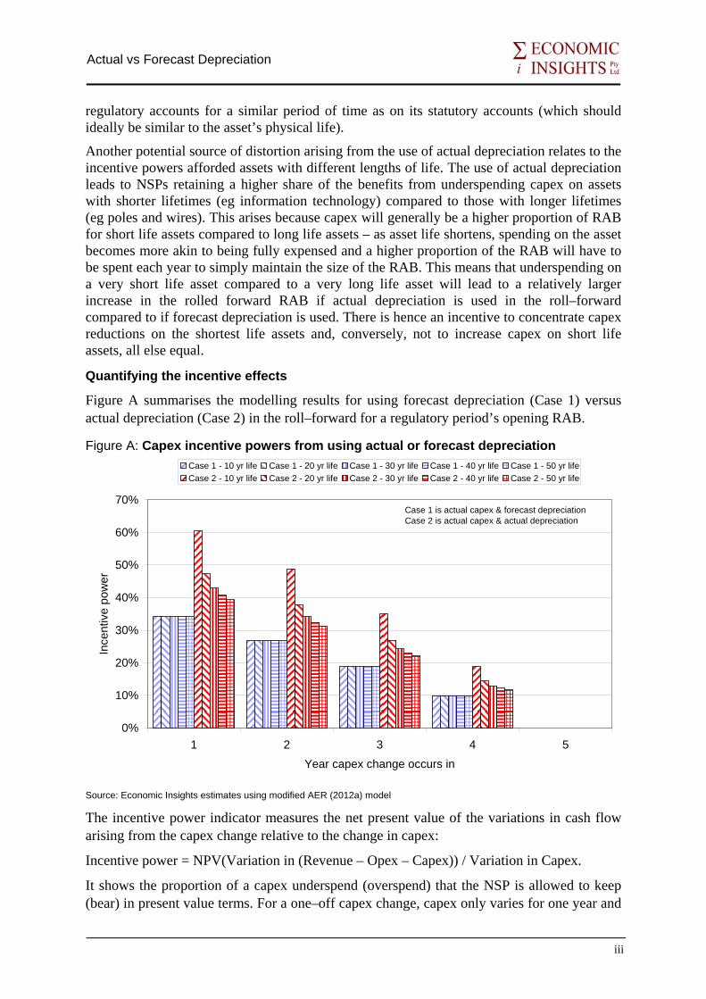
Figure A summarises the modelling results for using forecast depreciation (Case 1) versus actual depreciation (Case 2) in the roll–forward for a regulatory period’s opening RAB.
Figure A: Capex incentive powers from using actual or forecast depreciation
0%
10%
20%
30%
40%
50%
60%
70%
1 2 3 4 5Year capex change occurs in
Ince
ntiv
e po
wer
Case 1 - 10 yr life Case 1 - 20 yr life Case 1 - 30 yr life Case 1 - 40 yr life Case 1 - 50 yr lifeCase 2 - 10 yr life Case 2 - 20 yr life Case 2 - 30 yr life Case 2 - 40 yr life Case 2 - 50 yr life
Case 1 is actual capex & forecast depreciationCase 2 is actual capex & actual depreciation
Source: Economic Insights estimates using modified AER (2012a) model
The incentive power indicator measures the net present value of the variations in cash flow arising from the capex change relative to the change in capex:
Incentive power = NPV(Variation in (Revenue – Opex – Capex)) / Variation in Capex.
It shows the proportion of a capex underspend (overspend) that the NSP is allowed to keep (bear) in present value terms. For a one–off capex change, capex only varies for one year and
iii

Actual vs Forecast Depreciation
revenue will be unchanged in the current regulatory period (leading to a cash flow increase within the period for a capex reduction). But cash flow will also change in future periods when actual capex is used in the RAB roll–forward and further again when depreciation based on actual capex is used in the roll–forward as both lead to changes in the return of and return on capital components of future period revenues.
Figure A highlights the higher incentive power from using actual depreciation compared to forecast depreciation but the incentive using actual depreciation provides to concentrate capex reductions on shorter life assets. This incentive increases more than proportionally as the asset life reduces. Using forecast depreciation is lower powered but the incentive power does not vary with asset life. In both cases there is a higher incentive to defer capex in the early years of the regulatory period compared to the later years (in the absence of an EBSS).
One of the main arguments put forward in favour of using actual depreciation in the RAB roll–forward is that the current regulatory treatment of capex provides relatively weak incentives compared to opex leading to incentives being ‘unbalanced’ (eg AER 2010, p.461). However, the quantitative modelling shows that, in the absence of an EBSS, the incentive power for a one–off opex reduction is 100 per cent compared to an incentive power of between 30 and 40 per cent for a long life asset using either actual or forecast depreciation.
A comparison with a recurrent opex reduction is, however, likely to be more relevant as, unlike opex, a one–off reduction in capex will reduce the available capital stock in future years as well as the current year. In the first year of the regulatory period, the incentive power of a recurrent reduction in opex is 41 per cent which is little different from the incentive power of using either actual or forecast depreciation for long life assets. It is, however, less than the incentive power of 61 per cent for short life assets using actual depreciation.
Guidelines for exercising discretion
Whether the use of actual or forecast depreciation in the RAB roll–forward is more appropriate depends on a large number of factors and there is unlikely to be a ‘one size fits all’ answer. As a result it would be desirable to afford the AER flexibility in making the choice in transmission as well as in distribution. All stakeholders supported the AER having this flexibility and the analysis presented here concurs with that outcome. Similarly, it would be undesirable to prescribe the use of one method or the other in the rules.
Views differed, however, on whether the AER should be given additional guidance in making the choice between the two methods. To date the AER has used actual depreciation in all its electricity distribution reviews. This has been justified on the grounds of providing stronger capex incentives to redress imbalances relative to opex and to achieve consistency with transmission where actual depreciation was mandated.
The analysis in this report suggests that using forecast depreciation may be a preferable default as the use of actual depreciation is a second best substitute for having a capex EBSS, creates an incentive to substitute away from short life assets at a time when they may be becoming increasingly important to achieving efficient energy market outcomes and creates an incentive for NSPs to over–inflate their capex forecasts. This suggests that actual depreciation–based roll–forwards should be used sparingly and in response to special
iv

Actual vs Forecast Depreciation
circumstances where higher powered incentives are warranted but are not likely to create significant distortions in NSP input use.
Guidelines for the use of actual depreciation in the RAB roll–forward would take the following form:
• no capex EBSS in place
• demonstrated imbalance between opex and capex incentive powers
• demonstrated scope to substitute between opex and capex
• strong and effective service quality incentive scheme in place
• limited scope to substitute between new short and long life assets
• short life assets are a small part of capex requirements and of limited strategic importance, and
• regulator is able to adequately assess merits of proposed capex projects.
If these guidelines are not met then there is likely to be a strong case for forecast depreciation rather than actual depreciation being used in the RAB roll–forward.
v
Actual vs Forecast Depreciation
1 INTRODUCTION
The Australian Energy Market Commission (AEMC) is currently processing rule change requests from the Australian Energy Regulator (AER) and the Energy Users Rule Change Committee relating to the economic regulation of electricity network services. The rule changes sought by the AER include changes to:
• the capital and operating expenditure frameworks;
• the capital expenditure (capex) incentive arrangements; and
• the cost of capital (weighted average cost of capital - WACC) framework for determining the rate of return for network service providers.
The AEMC has asked Economic Insights Pty Ltd (‘Economic Insights’) to provide advice on the incentive effects of using actual versus forecast depreciation when rolling forward the regulated asset base (RAB) in energy network price regulation. This topic forms part of the capex incentive arrangements component of the proposed rule changes.
Specifically, the AEMC has asked Economic Insights to provide advice on:
• the impact on the incentives of a network service provider (NSP) of using actual or forecast depreciation to establish the NSP’s RAB;
• factors that should be considered in determining whether actual or forecast depreciation should be used to establish an NSP’s RAB; and
• the advantages and disadvantages of prescribing the use of actual or forecast depreciation in the National Electricity Rules (NER) and those of leaving it to the regulator’s discretion.
The AEMC has asked Economic Insights to consider:
• the theoretical/in–principle incentives created by using either actual or forecast depreciation to establish the opening RAB, including the impacts of using actual depreciation on incentives between short lived and long lived assets;
• approaches of Australian and international regulators in using actual or forecast depreciation and to comment on outcomes under different approaches; and
• whether there is a clearly superior approach and, if not, to explain the circumstances in which each approach works best.
In the following section we briefly review the process of building blocks price regulation and the part the opening RAB plays in it before reviewing relevant sections of the NER and the AER’s rule change proposal. In section 3 we analyse the theoretical incentive effects of the use of actual or forecast depreciation in forming the opening RAB before quantifying these incentive effects in section 4 using a range of regulatory models.
In section 5 we review recent regulatory practice and experience in Australia and overseas before examining stakeholders’ views presented in response to the current rule change proposal in section 6. Finally, we draw conclusions in section 7 and discuss conditions that might be placed on the use of one method or the other.
1

Actual vs Forecast Depreciation
2 BUILDING BLOCKS REGULATION AND THE NER
2.1 Building blocks regulation and the opening RAB
The building blocks approach to price regulation involves calculating an annual ‘revenue requirement’ for each NSP based on the costs it would incur if it was acting prudently. The costs are made up of opex, capital costs and a benchmark tax liability (which usually takes account of the differences between regulatory and taxation parameters and allowances). Capital costs are, in turn, made up of the return of capital and the return on capital. The return of capital is typically calculated as straight–line depreciation on the NSP’s opening RAB calculated over its estimated remaining life plus straight–line depreciation of assets added during the period calculated over their estimated total lives. The return on capital is the opening RAB multiplied by an opportunity cost rate. The opportunity cost rate is the weighted average cost of capital (WACC) which takes account of the different costs of the nominated debt and equity components of the RAB.
Financial capital maintenance (FCM) is a key principle in the building blocks approach. FCM means that a regulated business is compensated for prudent expenditure and prudent investments such that, on an ex–ante basis, its financial capital is at least maintained in present value terms.
Since the building blocks method involves setting the price cap for each NSP at the start of the regulatory period, forecasts have to be made of the annual revenue requirement stream over the coming regulatory period and of the quantities of outputs that will be sold over that period. Since the opening RAB for the regulatory period will be (largely) known, the annual revenue requirements for the upcoming regulatory period can be forecast based on forecasts of opex and capex.
Once the forecasts of annual revenue requirements and output quantities have been made, the P0 and X factors are set so that the net present value of the forecast operating revenue stream over the upcoming regulatory period is equated with the net present value of the forecast annual revenue requirement stream.
Regulators in different jurisdictions have applied slightly different variants of the building blocks method. The main differences are timing assumptions regarding capex (ie when assets added each year actually come into service), whether a real WACC is used or, alternatively, a nominal WACC is used but revaluation gains are then deducted so that inflation is not allowed for twice and how the opening RAB for the subsequent regulatory period is formed.
In energy network industries the market value of assets at any one time is not well defined. A large part of the asset base comprises sunk assets that are not regularly traded between competitors. In principle their value is the present value of their future services, but this is a matter partly determined by the regulator. In this context, asset values can be updated over time using a number of different methods including periodic revaluations and more mechanical ‘roll forward’ mechanisms. Periodic revaluations are typically done using the depreciated optimised replacement cost (DORC) method but can introduce a degree of volatility and uncertainty due to the partly subjective nature of DORC valuation decisions.
2
Actual vs Forecast Depreciation
The term ‘roll-forward’ refers to how the asset base is adjusted over time to reflect new investment in the business and changes in the productive capability and value of the existing asset base (IPART 1999). It usually involves adding capital expenditure (capex) and subtracting depreciation from an original RAB valuation to roll it forward from year to year. This process improves the predictability and certainty of forming the opening RAB for future regulatory periods and reduces the scope for windfall gains and losses resulting from subjective valuation decisions. However, a number of decisions still have to be made.
Forecast capex and depreciation at review time will inevitably deviate from subsequently realised capex and depreciation patterns through the regulatory period. In principle, either the originally forecast series or the subsequently realised or actual capex and depreciation series could be used in the roll forward. Which combination of actual and forecast capex and depreciation is used has important implications for the incentive properties of the regulatory regime as will be demonstrated in sections 3 and 4.
By way of example, under the AER’s (2008b) Roll Forward Model (RFM) actual capex and depreciation for a regulatory period are recognised at the time of the next review and incorporated in the opening RAB for the next regulatory period. That is, if NSPs end up spending less capex than forecast at the start of the regulatory period then their opening RAB for the next regulatory period will be correspondingly higher if actual depreciation is used in the roll forward compared to using forecast depreciation for the preceding regulatory period (given that actual capex is required to be used in the roll–forward). Conversely, if NSPs spend more capex than forecast at the start of the regulatory period then their opening RAB for the next regulatory period will be correspondingly lower if actual depreciation is used in the roll forward compared to using forecast depreciation for the preceding regulatory period.
When making a distribution determination, the AER can decide whether, when rolling forward the RAB from the date of the determination to the commencement of the following regulatory control period, depreciation on actual or forecast capital expenditure should be used. The AER is seeking a similar discretion with respect to electricity transmission.
2.2 Relevant provisions of the NER
Chapter 6 of the NER covers the economic regulation of distribution services, while Chapter 6A covers transmission services. The NER requires the AER to produce a roll-forward model (cl.6.5.1) and specifies the essential elements of the roll–forward to establish the value of the RAB at the beginning of the first year of a regulatory period.1 The NER maps out the perpetual inventory model in current value terms:
(1)
where At is the asset value at the beginning of period t; π is the rate of inflation; NI is net investment (ie capex less asset disposals); and DA is depreciation. Specifically:
1 The RAB for the ‘distribution system’ of an NSP is the value of only those assets used to provide standard control services. Quantities of capex and depreciation likewise only refer to assets properly allocated to standard control services (S6.2.1(f)).
3
Actual vs Forecast Depreciation
• The RAB determined at the beginning of the previous regulatory period: if there was any estimated capital expenditure in the previous value of the RAB (relating to part of the period before the preceding regulatory period), then it must be replaced by the actual capex for the same period. The adjustment must also remove any benefit or penalty associated with any difference between the estimated and actual capex (S6.2.1(e)(3)). This will result in an adjusted starting value of the RAB for the roll–forward.
• The roll–forward is calculated on a yearly basis over each of the years of the preceding regulatory period (6.5.1(e)(2)).
• Each year the RAB is adjusted for actual inflation, consistent with the indexation for the control mechanism in the previous control period (eg CPI, if CPI–X is used) (6.5.1(e)(3)). By implication the assets cannot be revalued in another way.
• NI is the actual capex, less the disposal value of any asset sold, for that part of the preceding regulatory period for which actual capex data is available. Where actual capex data is not available, the amount of capex previously approved by the AER for that period must be used in the roll forward. (S6.2.1(e)(1)&(2))
• DA is the amount of depreciation during the previous regulatory control period, ‘calculated according to the distribution determination for that period’. (S6.2.1(e)(5)).
For distribution the discretionary element in this formula relates to depreciation via the requirement that depreciation be ‘calculated according to the distribution determination for that period’. Two different aspects of the NER govern the determination of depreciation:
a) When making a determination, the AER must decide whether the depreciation to be used when rolling forward the RAB from the date of the determination to the commencement of the following regulatory control period, should be the depreciation on actual or forecast capital expenditure. (6.12.1(18))2
b) The AER must approve the depreciation schedules proposed by a utility if they comply with the following requirements:
i. use a depreciation profile that reflects the nature of the assets or category of assets
ii. the depreciation charges (in real terms) add up to the original investment over the life of the asset
iii. once set, the depreciation schedule should remain consistent over subsequent regulatory reviews. (6.5.5)
If the AER were to elect, under (a), to use the depreciation on forecast capex in the RAB roll–forward, then for that capex it would likely have difficulty complying with either (b)(ii) or (iii). That is, having departed from the originally approved depreciation profile, the regulator would need to either amend that profile in subsequent periods in order to ensure that it adds up to the original investment over the life of the asset or, if not, accept that total depreciation charges over the life of the asset would not add up to the original investment. 2 Total depreciation over the previous control period includes: (a) the depreciation on the previous value of the RAB over that period; and (b) depreciation on the capex during that period. The AER’s discretion to choose the forecast depreciation for the roll forward only relates to (b) – depreciation associated with the capex during the period.
4
Actual vs Forecast Depreciation
These two options broadly conform with FCM on an ex–post basis and an ex–ante basis, respectively. It should be noted that under the first approach there would not be any affect on the NSP of using forecast depreciation in place of actual depreciation (on a present value basis), consistent with the following observation from the ACCC (2001, p.10):
‘… as depreciation is intended to represent the return of capital expenditures over the life of the asset, accumulated depreciation should not exceed the initial actual capital cost of the infrastructure. Apart from this requirement not to double count, the time path for depreciation can be viewed as arbitrary. As long as the rate of return on the residual RAB value at any point in time is expected to be achieved, the NPV of expected cash flows will equate to the RAB.’
The framework for electricity transmission in Chapter 6A differs by requiring actual depreciation to be used.
Some of the issues raised in relation to the roll–forward formula in the AER’s rule change proposal and submissions to the AEMC relate to the incentives of NSPs to submit reasonable forecasts of capex requirements. The rules pertaining to the submission and approval of these forecasts are, therefore, relevant.
The NER require the AER to approve a producer’s capex forecast if it meets the criteria of being:
• an economically efficient investment
• prudent, and
• based on reasonable assumptions (eg input prices and demand forecasts).
The AER is required to reject the NSP’s capex forecast unless it is satisfied that the forecast meets the above capex criteria (cl. 6.5.6(d) & 6.5.7(d)). The Australian Competition Tribunal (2010, paras 69–71) has previously ruled on this as follows (in the context of comparable opex criteria):
‘… the very nature of forecasting means that there can be no one absolute or perfect figure. ... Simply because there is a range of forecasts and a DNSP’s forecast falls within the range does not mean it must be accepted when … the AER has sound reason for rejecting the forecast. … cl 6.5.6(c) of the Rules does not require the AER to identify a range of forecasts and determine whether a DNSP’s figure falls within that range. Nor is there anything in the legislation under consideration here that requires the AER to accept a figure advanced by a DNSP simply because it may be within a range of figures the DNSP may point to as reasonable. … what cl 6.5.6(c) requires is the AER to accept a forecast if it is satisfied that the forecast reasonably reflects the opex criteria.’
2.3 The AER’s rule change proposal for depreciation in the roll–forward
Chapter 6A of the NER currently requires the AER to use actual depreciation for TNSPs:
‘The previous value of the regulatory asset base must be reduced by the amount of actual depreciation of the regulatory asset base during the previous control
5

Actual vs Forecast Depreciation
period, calculated in accordance with the rates and methodologies allowed in the transmission determination (if any) for that period.’ (S6A.2.1(f)(5))
The AER rule change proposal proposes to delete the word ‘actual’ from this section and require the regulator to specify the use of either actual or forecast depreciation for the RAB roll–forward so that the treatment of transmission in the rules becomes consistent with that of distribution.
The AER (2011, p.44) argues that it should be given the flexibility to adopt either a high powered or a lower powered depreciation incentive to achieve a balanced capex incentive framework. The AER goes on to note that where forecast depreciation is used the amount of depreciation included in the RAB roll–forward does not vary with actual capex outcomes during the period and the calculation of depreciation does not add to the strength of the capex incentive framework. The AER also noted that the current framework relies predominantly on the use of actual depreciation to strengthen otherwise very low powered capex incentives.
The AER (2011, p.45) noted the following potential problems with the current framework based on actual depreciation:
‘An important consideration in the choice between the use of actual or forecast depreciation is whether any differences between the actual and forecast outcomes are likely to be driven by permanent efficiency improvements or whether they reflect uncontrollable factors or the temporary deferral of investments. If the differences are likely to result from uncontrollable factors, the temporary deferral of investments or the systematic over–forecasting of capex, then the use of actual depreciation will result in higher windfall gains/losses than if forecast depreciation is adopted.
‘The AEMC considered that a relatively low powered capex incentive paired with a higher powered opex incentive may distort TNSPs use of inputs, thereby creating productive inefficiencies. In contrast, MCE determined it was appropriate for the AER to have the discretion in relation to distribution determinations to adopt either forecast or actual depreciation.’
Allowing flexibility in the use of actual or forecast depreciation for transmission services also was argued to have the following benefits (AER 2011, p.46):
‘… when a significant proportion of the forecast capex reflects uncontrollable factors, forecast depreciation could apply, reducing the prospect of windfall gains and losses. This would ensure that the TNSP is not rewarded for cost reductions which do not reflect cost efficiencies, or unduly penalised for circumstances outside its control.’
6
Actual vs Forecast Depreciation
3 THEORETICAL INCENTIVE EFFECTS
3.1 General incentive considerations A limitation of the incentives provided under the building blocks framework is that the regulator will base its assessment largely on the cost outturns of the regulated business. Knowing this, when the regulated firm chooses its cost level it will have regard not only to its immediate profits, but also the influence its cost choice will have on its regulatory cost proposal at the next round. For example, if the regulated firm were to achieve full opex efficiency in the short term, this would undermine its future regulatory proposal and diminish surplus profits attainable in the next period. But if it never reduced opex, it would never achieve those extra profits. Hence cost efficiency incentives are weakened only, not removed altogether.
The incentives relating to capex are quite different. If a firm reduces its capex in the short term, it may strengthen its case for a higher capex allowance in the next period. This may occur if the reduced capex in the short term is not due to superior cost management in capital projects, but due to deferral of projects, which increasingly become bunched into the next regulatory period. To the extent these projects are necessary to maintain supply quality standards, the regulator may feel compelled to allow them at the next review. This could potentially become a process of ‘double dipping’.
There are thus two important issues with respect to capex incentives: the incentive to submit reasonable forecasts and the incentive to carry out efficient levels of investment. The two are related because future regulatory decisions will be influenced by current capex activity, just as they will be influenced by forecasts submitted at future price reviews. However, they are also quite distinct in another respect. As the previous section highlights, the AER has considerable capacity to manage the risk associated with unreasonable capex forecasts being presented to it. However, once the determination is made, the AER has no direct influence on the capex activity of the business, and must rely entirely on the incentives within the framework to produce outcomes consistent with the objectives.
The general approach to incentives, like performance measurement, may be outcome–oriented or input–oriented. An outcome–based incentive framework for investment efficiency would be related to indicators of reliability, supply security (ie capacity) and other network performance attributes. If rewards and penalties are appropriately structured, and there is a sufficiently close relationship between investment activity and the outcome indicators, then such an incentive framework might be relied on to ensure there would be sufficient capex. Conventional cost efficiency incentives would then be relied on to minimise the amount of capex subject to achieving acceptable outcomes for reliability and security of supply.
Input–based incentive mechanisms attempt to identify the appropriate levels of inputs that the regulated business should use and then provide incentives for the firm that encourage it to use those amounts of inputs.
There are likely to be two general regulatory aims with regard to capex. Firstly, that the quantity of capital inputs will be adequate to ensure that the reliability, safety and quality of network services meet the standards expected by the regulator or consumers. Secondly, that the cost of that capex be minimised through appropriate choices of projects, inputs and technologies, and using appropriate organisational, project and risk management. Given these
7
Actual vs Forecast Depreciation
two broad targets, there will need to be at least two effective incentive mechanisms directed toward achieving them. The first mechanisms might be derived from a suitable ‘service quality’ incentive mechanism, in which regulated businesses are rewarded or penalised for performance against clearly defined standards of network reliability, safety and supply security. The effectiveness of a mechanism of this kind would depend on a clear relationship between capex and standards of service.
The AER’s choice of actual or forecast depreciation in the RAB roll–forward will influence the incentives for NSPs to undertake capex. However, those incentives need to be considered within the context of the overall incentives provided by all elements of the regulation framework for capex. For example, in the absence of an efficiency benefit sharing scheme (EBSS) for capex, NSPs will have an incentive to underspend capex in the early years of a regulatory period compared to the later years because they can retain the benefits of the underspend for longer. An EBSS will be the first best way of addressing this distortion. Capex incentives resulting from different treatments of depreciation in the RAB roll–forward could have the effect of exacerbating the incentive to underspend in the early years of the regulatory period. It is therefore important to assess incentives arising from the overall regulatory regime when deciding on the appropriate treatment of depreciation in the roll–forward. However, these broader issues are beyond the scope of this project which focuses specifically on the treatment of depreciation.
The use of actual depreciation can generally be expected to provide higher powered incentives for constraining capex growth. This arises because if the NSP underspends its forecast capex during a regulatory period, it keeps the benefit of the higher forecast depreciation allowance within period while also having a smaller write–down of the opening RAB for the next regulatory period than would be the case if the RAB roll–forward was done on the basis of the forecast depreciation (where the forecast was set at the start of the preceding regulatory period). The NSP is then able to obtain a return on a higher RAB in subsequent regulatory periods than would be the case had forecast depreciation been used.
Conversely, if the NSP overspends its capex forecast then it has a lower depreciation allowance within the regulatory period than its actual depreciation and also has its rolled–forward RAB for the start of the next regulatory period written–down more when actual depreciation is used in the roll–forward than when the original forecast depreciation is used.
As a result, the use of actual depreciation in the roll–forward provides more incentive for the NSP to underspend its forecast capex and/or to contain the size of any overspend than does the use of forecast capex, all else equal.
However, higher powered incentives associated with using actual depreciation have to be offset against a number of potential distortionary effects. These include an incentive for NSPs to overinflate their capex forecasts at the start of the regulatory period. Since the NSP will obtain a benefit from underspending its forecast capex if actual depreciation is subsequently used as the basis of the RAB roll–forward, it will be in the NSP’s interests to exploit its information asymmetry and persuade the regulator that its capex requirements for the coming period will be higher than they really are. This would lead to consumers paying more than they need to. Conversely, if the originally forecast depreciation is used in the roll–forward then the NSP has an incentive, compared to using actual depreciation, to ensure its capex forecasts at the start of the period are relatively accurate so that the asset stays on the regulatory accounts for a similar period of time as on its statutory accounts (which should ideally be similar to the asset’s physical life).
8
Actual vs Forecast Depreciation
Another potential source of distortion arising from the use of actual depreciation can relate to the powers of incentive afforded assets with different lengths of life. The use of actual depreciation is likely to lead to NSPs retaining a higher share of the benefits from underspending capex on assets with shorter lifetimes (such as information technology and general items) compared to those with longer lifetimes (such as poles and wires). This arises because capex will generally be a higher proportion of RAB for short–lived assets (taken in isolation) compared to long–lived assets (also taken in isolation) – as asset life shortens, spending on the asset becomes more akin to being fully expensed and a higher proportion of its RAB will have to be spent each year to simply maintain the size of its RAB. For example, assuming an even distribution of asset ages, an asset with a 5 year life would require annual real capex equivalent to 20 per cent of its RAB to maintain a constant real RAB for that asset. An asset with a 50 year life, on the other hand, would only require annual real capex equivalent to 2 per cent of its RAB to maintain a constant real RAB for that asset.
This means that underspending on a very short life asset compared to a very long life asset will lead to a relatively larger increase in the rolled forward RAB for that asset if actual depreciation is used in the roll–forward compared to if forecast depreciation is used. Continuing with the example above, a 10 per cent reduction in real capex for the 5 year life asset would have a 2 per cent impact on the RAB for that asset (from the depreciation side) but a 10 per cent reduction in real capex for the 50 year life asset would only have a 0.2 per cent impact on the RAB for that asset. There is hence an incentive to concentrate capex reductions on the shortest life assets and, conversely, not to increase capex on short life assets, all else equal.
3.2 Financial capital maintenance and depreciation–related incentives
As noted in section 2.1, FCM is a key principle embedded in the building blocks approach. FCM means that a regulated business is compensated for prudent expenditure and prudent investments such that its financial capital is at least maintained in present value terms. However, there are a variety of ways in which FCM can be interpreted and implemented and these have important implications for the incentive power of the regulatory regime.
In its purest form, FCM can be implemented on an ex–post basis so that the NSP is fully compensated at all times for its actual expenditure. However, the NSP would then face no incentive to provide services of a given quality or to reduce its opex and capex. This would be equivalent to an extreme form of rate of return regulation. Incentive regulation, on the other hand, is predicated on deviation from the principal of ex–post FCM to reward or penalise the NSP as a means of promoting specified objectives. The incentive properties of a regime then depend on how much the NSP’s revenue stream deviates from that required for ex–post FCM.
While departure from ex–post FCM in practice could be considered a windfall gain (or loss) to the NSP, it is precisely such windfall gains and losses that are required if incentives are to be provided to achieve desired outcomes. However, conversely, the regulator needs to ensure that departures from ex–post FCM do in fact yield the required incentives. In practice, the regulator tries to achieve this by the use of ex–ante FCM. That is, the regulator provides regulatory opex and capex allowances and opening RABs based on its estimates of likely efficient costs and the NSP then has an incentive to better these allowances. If the NSP can
9
Actual vs Forecast Depreciation
achieve lower opex and capex costs then it keeps the benefits for a specified period. Conversely, if it exceeds the ex–ante allowances then it bears the cost of the excess expenditure for a specified period. This process provides an incentive for the NSP to reveal its true efficient costs over time and, in principle, reduces the degree of information asymmetry between the NSP and the regulator.
At the start of a regulatory period the regulator forecasts the NSP’s capex over the coming period and gives the NSP a depreciation allowance, usually based on the straight–line method. This allows the regulator to set the return on and return of capital building block components for the upcoming period. Under the RAB roll–forward approach, at the start of the next regulatory period, the regulator observes the actual capex from the last period and decides on how much capex and depreciation will be rolled into the opening RAB for the next period using the formula:
(2) Opening RAB next period = Opening RAB last period + Capex allowance last period – Depreciation allowance last period.
Biggar (2004, p.3) noted that the incentive properties emanating from the RAB roll–forward depend on how the capex and depreciation allowances included in the roll–forward depend on actual versus forecast capex and depreciation, respectively. It is instructive to examine the four key combinations as follows: actual capex and forecast depreciation; actual capex and actual depreciation; forecast capex and forecast depreciation; forecast capex and actual depreciation.
Case 1: Roll–forward using actual capex and forecast depreciation
Using a stylised model, Biggar (2004, p.16) shows that using actual capex and forecast depreciation in the roll–forward is equivalent to imposing ex–post FCM and thus has low powered incentive properties.
Suppose that Kt–1 is the opening RAB, It and Ot are actual capex and opex, respectively, and IFt and OFt are forecast capex and opex, respectively. Furthermore, let forecast depreciation be a function of forecast capex so that DFt = f(IFt). The allowed revenue stream is then RFt = rKt–1 + OFt – f(IFt) where r is the allowed cost of capital.
Ex–post FCM will apply when:
(3) Kt = (1 + r)Kt + Ot + It – RFt = Kt–1 + It – f(IFt) + (Ot – OFt)
That is, ex–post FCM applies when the opening RAB for the next period is equal to the opening RAB for the previous regulatory period plus actual capex less forecast depreciation plus the difference between actual and forecast opex for the last regulatory period.
In this case the NSP faces no incentive to reduce its capex but also receives no benefit from increasing its capex forecast.
Case 2: Roll–forward using actual capex and actual depreciation
Using the actual capex and actual depreciation combination is equivalent to ‘partial’ ex–ante FCM where the NSP is allowed to keep some of the benefits of reducing actual capex relative to that originally forecast.
10
Actual vs Forecast Depreciation
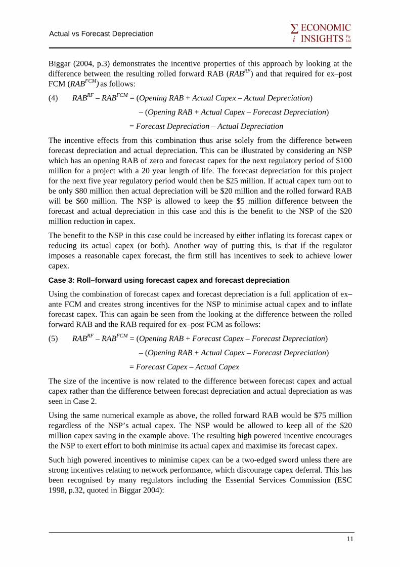
Biggar (2004, p.3) demonstrates the incentive properties of this approach by looking at the difference between the resulting rolled forward RAB (RABRF) and that required for ex–post FCM (RABFCM) as follows:
(4) RABRF – RABFCM = (Opening RAB + Actual Capex – Actual Depreciation)
– (Opening RAB + Actual Capex – Forecast Depreciation)
= Forecast Depreciation – Actual Depreciation
The incentive effects from this combination thus arise solely from the difference between forecast depreciation and actual depreciation. This can be illustrated by considering an NSP which has an opening RAB of zero and forecast capex for the next regulatory period of $100 million for a project with a 20 year length of life. The forecast depreciation for this project for the next five year regulatory period would then be $25 million. If actual capex turn out to be only $80 million then actual depreciation will be $20 million and the rolled forward RAB will be $60 million. The NSP is allowed to keep the $5 million difference between the forecast and actual depreciation in this case and this is the benefit to the NSP of the $20 million reduction in capex.
The benefit to the NSP in this case could be increased by either inflating its forecast capex or reducing its actual capex (or both). Another way of putting this, is that if the regulator imposes a reasonable capex forecast, the firm still has incentives to seek to achieve lower capex.
Case 3: Roll–forward using forecast capex and forecast depreciation
Using the combination of forecast capex and forecast depreciation is a full application of ex–ante FCM and creates strong incentives for the NSP to minimise actual capex and to inflate forecast capex. This can again be seen from the looking at the difference between the rolled forward RAB and the RAB required for ex–post FCM as follows:
(5) RABRF – RABFCM = (Opening RAB + Forecast Capex – Forecast Depreciation)
– (Opening RAB + Actual Capex – Forecast Depreciation)
= Forecast Capex – Actual Capex
The size of the incentive is now related to the difference between forecast capex and actual capex rather than the difference between forecast depreciation and actual depreciation as was seen in Case 2.
Using the same numerical example as above, the rolled forward RAB would be $75 million regardless of the NSP’s actual capex. The NSP would be allowed to keep all of the $20 million capex saving in the example above. The resulting high powered incentive encourages the NSP to exert effort to both minimise its actual capex and maximise its forecast capex.
Such high powered incentives to minimise capex can be a two-edged sword unless there are strong incentives relating to network performance, which discourage capex deferral. This has been recognised by many regulators including the Essential Services Commission (ESC 1998, p.32, quoted in Biggar 2004):
11
Actual vs Forecast Depreciation
‘One alternative would be to roll forward the projected capital expenditure for the current period. … The difficulty with this approach is that it would provide a strong incentive for licensees to inflate their future projections of necessary capital expenditure. It may also encourage under-spending on network maintenance and replacement programmes, risking a deterioration in service performance which may only manifest itself after a long time lag.’
Similarly, when reviewing the first five–year period of UK electricity distribution regulation, Ofgem (1999, p.11, quoted in Biggar 2004) expressed concern that high powered incentives for cost efficiency induced firms to sacrifice longer run service quality as follows:
‘The focus [of regulated NSPs] appears to be on beating the projections on which the price control was based rather than on meeting objective standards at minimum cost and having a continuous incentive to outperform peers in the cost and quality of outputs.’
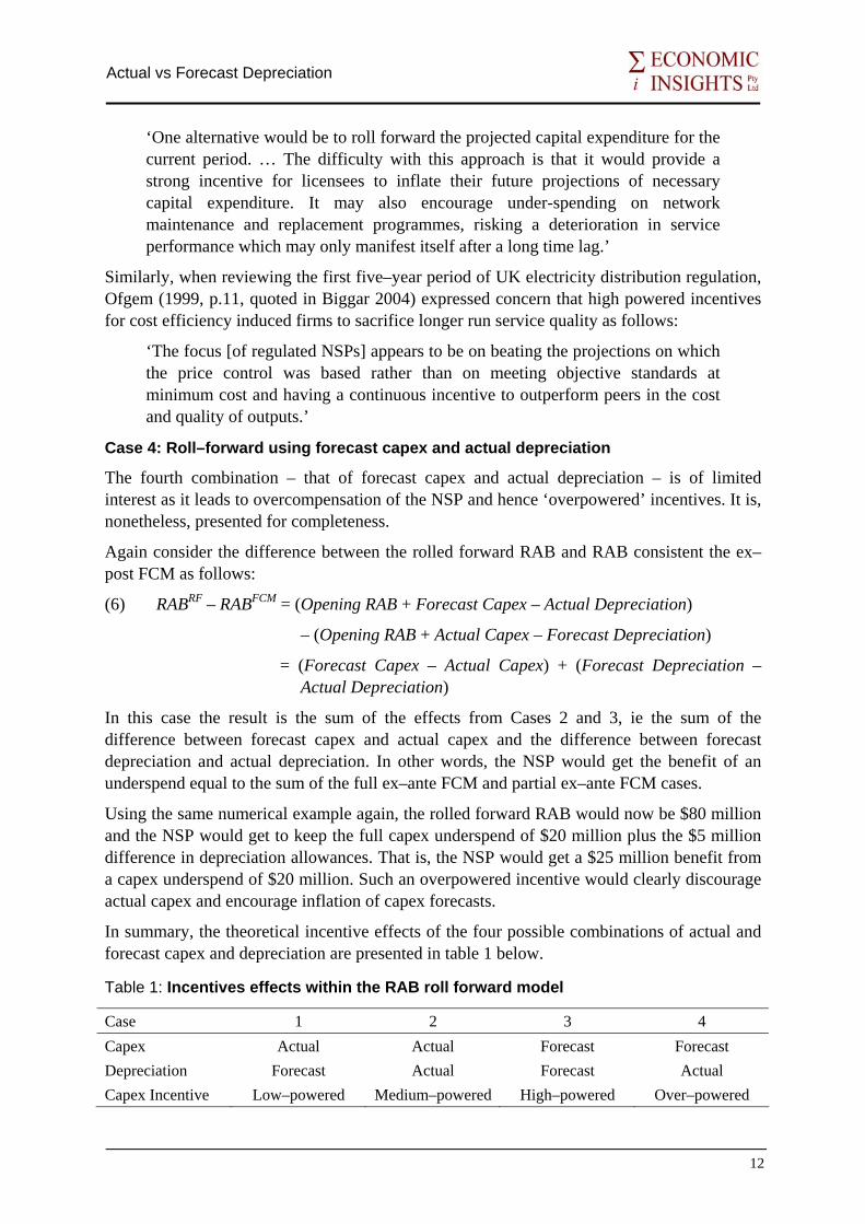
Case 4: Roll–forward using forecast capex and actual depreciation
The fourth combination – that of forecast capex and actual depreciation – is of limited interest as it leads to overcompensation of the NSP and hence ‘overpowered’ incentives. It is, nonetheless, presented for completeness.
Again consider the difference between the rolled forward RAB and RAB consistent the ex–post FCM as follows:
(6) RABRF – RABFCM = (Opening RAB + Forecast Capex – Actual Depreciation)
– (Opening RAB + Actual Capex – Forecast Depreciation)
= (Forecast Capex – Actual Capex) + (Forecast Depreciation – Actual Depreciation)
In this case the result is the sum of the effects from Cases 2 and 3, ie the sum of the difference between forecast capex and actual capex and the difference between forecast depreciation and actual depreciation. In other words, the NSP would get the benefit of an underspend equal to the sum of the full ex–ante FCM and partial ex–ante FCM cases.
Using the same numerical example again, the rolled forward RAB would now be $80 million and the NSP would get to keep the full capex underspend of $20 million plus the $5 million difference in depreciation allowances. That is, the NSP would get a $25 million benefit from a capex underspend of $20 million. Such an overpowered incentive would clearly discourage actual capex and encourage inflation of capex forecasts.
In summary, the theoretical incentive effects of the four possible combinations of actual and forecast capex and depreciation are presented in table 1 below.
Table 1: Incentives effects within the RAB roll forward model
Case 1 2 3 4 Capex Actual Actual Forecast Forecast Depreciation Forecast Actual Forecast Actual Capex Incentive Low–powered Medium–powered High–powered Over–powered
12

Actual vs Forecast Depreciation
This analysis suggests that a move from the use of actual capex and actual depreciation to using actual capex and forecast depreciation in the RAB roll–forward would reduce the incentive for NSPs to inflate their capex forecasts but would weaken capex efficiency incentives and effectively impose ex–post FCM which is commonly associated with rate of return regulation.
We turn now to quantitative estimates of the incentive effects of the different options.
13
Actual vs Forecast Depreciation
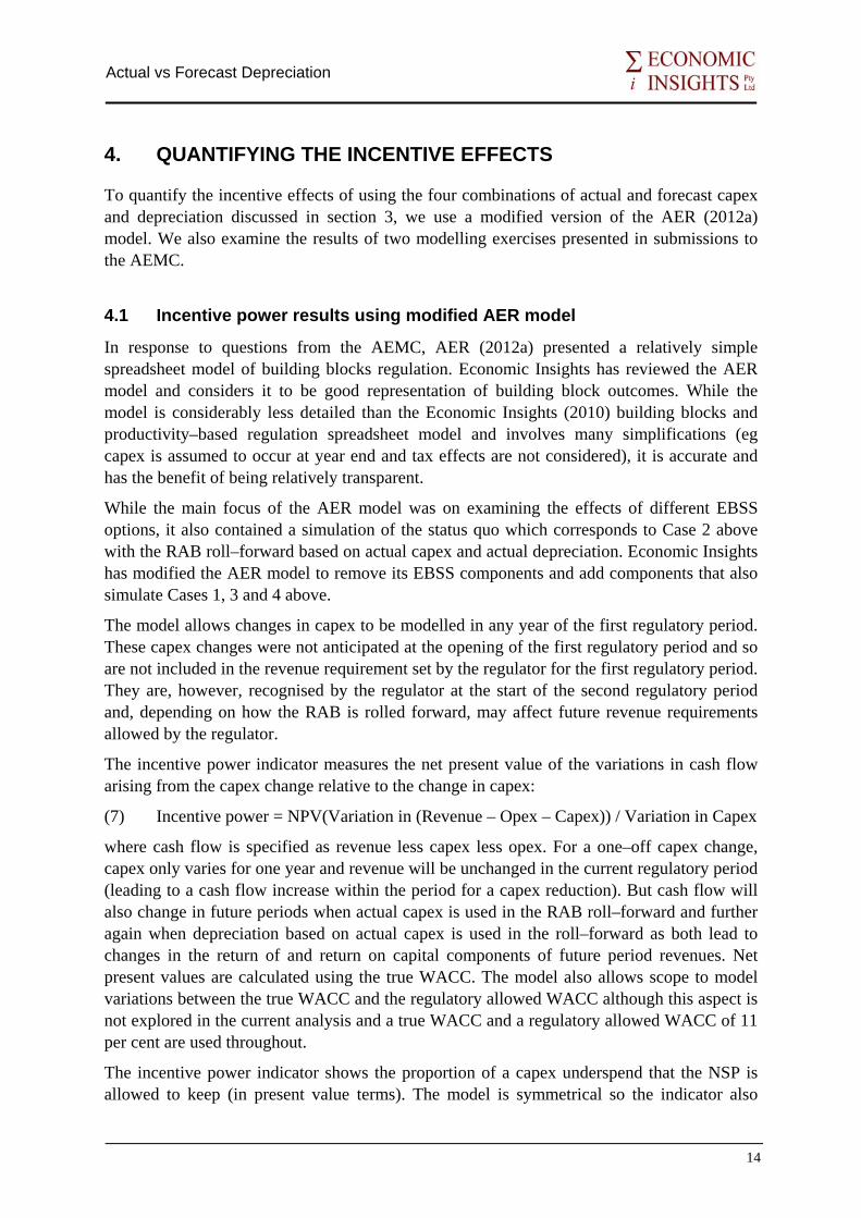
4. QUANTIFYING THE INCENTIVE EFFECTS
To quantify the incentive effects of using the four combinations of actual and forecast capex and depreciation discussed in section 3, we use a modified version of the AER (2012a) model. We also examine the results of two modelling exercises presented in submissions to the AEMC.
4.1 Incentive power results using modified AER model
In response to questions from the AEMC, AER (2012a) presented a relatively simple spreadsheet model of building blocks regulation. Economic Insights has reviewed the AER model and considers it to be good representation of building block outcomes. While the model is considerably less detailed than the Economic Insights (2010) building blocks and productivity–based regulation spreadsheet model and involves many simplifications (eg capex is assumed to occur at year end and tax effects are not considered), it is accurate and has the benefit of being relatively transparent.
While the main focus of the AER model was on examining the effects of different EBSS options, it also contained a simulation of the status quo which corresponds to Case 2 above with the RAB roll–forward based on actual capex and actual depreciation. Economic Insights has modified the AER model to remove its EBSS components and add components that also simulate Cases 1, 3 and 4 above.
The model allows changes in capex to be modelled in any year of the first regulatory period. These capex changes were not anticipated at the opening of the first regulatory period and so are not included in the revenue requirement set by the regulator for the first regulatory period. They are, however, recognised by the regulator at the start of the second regulatory period and, depending on how the RAB is rolled forward, may affect future revenue requirements allowed by the regulator.
The incentive power indicator measures the net present value of the variations in cash flow arising from the capex change relative to the change in capex:
(7) Incentive power = NPV(Variation in (Revenue – Opex – Capex)) / Variation in Capex
where cash flow is specified as revenue less capex less opex. For a one–off capex change, capex only varies for one year and revenue will be unchanged in the current regulatory period (leading to a cash flow increase within the period for a capex reduction). But cash flow will also change in future periods when actual capex is used in the RAB roll–forward and further again when depreciation based on actual capex is used in the roll–forward as both lead to changes in the return of and return on capital components of future period revenues. Net present values are calculated using the true WACC. The model also allows scope to model variations between the true WACC and the regulatory allowed WACC although this aspect is not explored in the current analysis and a true WACC and a regulatory allowed WACC of 11 per cent are used throughout.
The incentive power indicator shows the proportion of a capex underspend that the NSP is allowed to keep (in present value terms). The model is symmetrical so the indicator also
14
Actual vs Forecast Depreciation
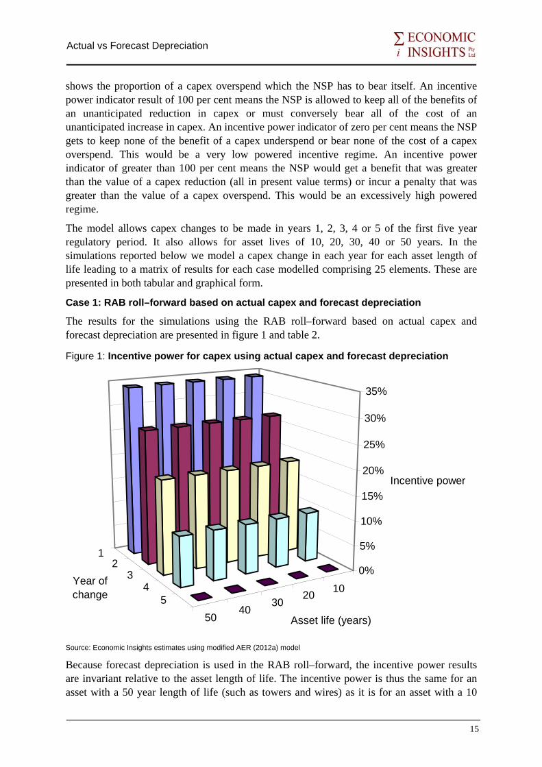
shows the proportion of a capex overspend which the NSP has to bear itself. An incentive power indicator result of 100 per cent means the NSP is allowed to keep all of the benefits of an unanticipated reduction in capex or must conversely bear all of the cost of an unanticipated increase in capex. An incentive power indicator of zero per cent means the NSP gets to keep none of the benefit of a capex underspend or bear none of the cost of a capex overspend. This would be a very low powered incentive regime. An incentive power indicator of greater than 100 per cent means the NSP would get a benefit that was greater than the value of a capex reduction (all in present value terms) or incur a penalty that was greater than the value of a capex overspend. This would be an excessively high powered regime.
The model allows capex changes to be made in years 1, 2, 3, 4 or 5 of the first five year regulatory period. It also allows for asset lives of 10, 20, 30, 40 or 50 years. In the simulations reported below we model a capex change in each year for each asset length of life leading to a matrix of results for each case modelled comprising 25 elements. These are presented in both tabular and graphical form.
Case 1: RAB roll–forward based on actual capex and forecast depreciation
The results for the simulations using the RAB roll–forward based on actual capex and forecast depreciation are presented in figure 1 and table 2.
Figure 1: Incentive power for capex using actual capex and forecast depreciation
102030
4050
12
34
5
0%
5%
10%
15%
20%
25%
30%
35%
Incentive power
Asset life (years)
Year of change
Source: Economic Insights estimates using modified AER (2012a) model
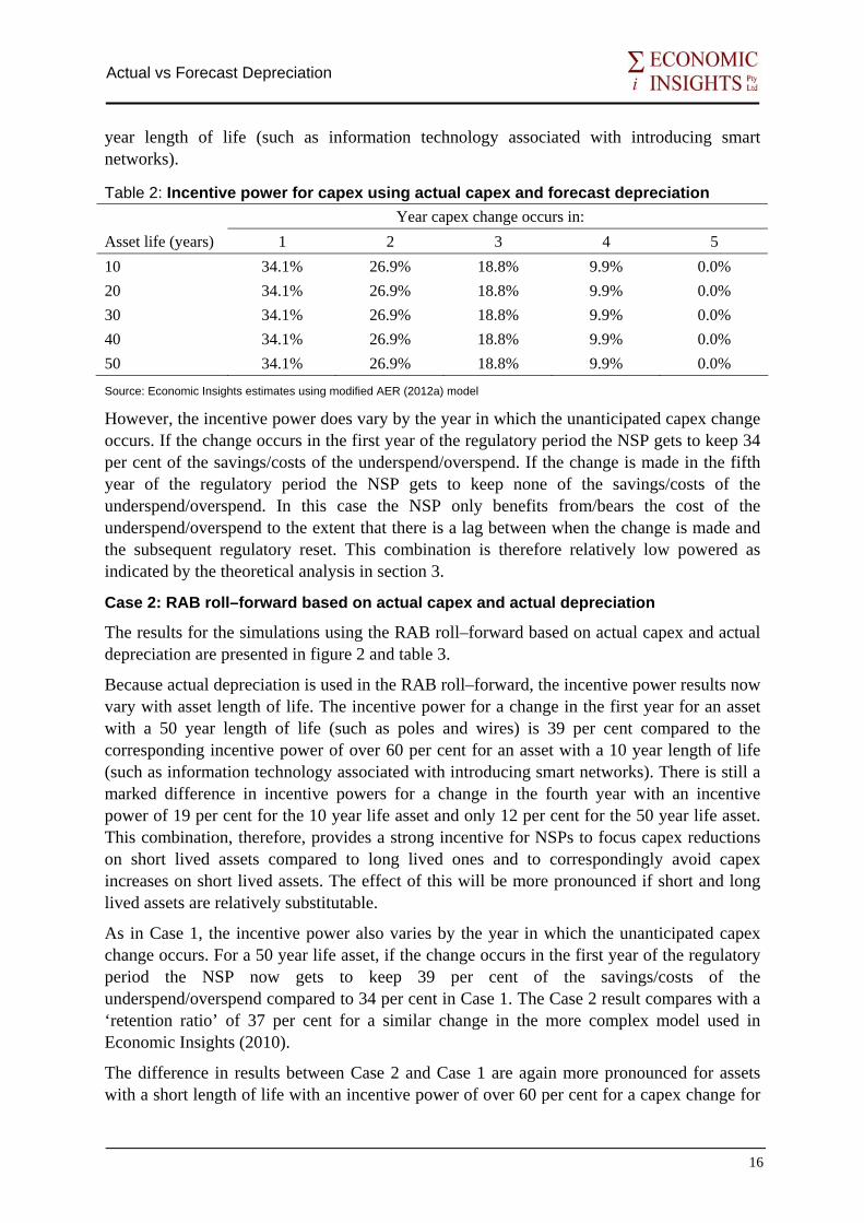
Because forecast depreciation is used in the RAB roll–forward, the incentive power results are invariant relative to the asset length of life. The incentive power is thus the same for an asset with a 50 year length of life (such as towers and wires) as it is for an asset with a 10
15
Actual vs Forecast Depreciation
year length of life (such as information technology associated with introducing smart networks).
Table 2: Incentive power for capex using actual capex and forecast depreciation Year capex change occurs in: Asset life (years) 1 2 3 4 5 10 34.1% 26.9% 18.8% 9.9% 0.0% 20 34.1% 26.9% 18.8% 9.9% 0.0% 30 34.1% 26.9% 18.8% 9.9% 0.0% 40 34.1% 26.9% 18.8% 9.9% 0.0% 50 34.1% 26.9% 18.8% 9.9% 0.0%
Source: Economic Insights estimates using modified AER (2012a) model
However, the incentive power does vary by the year in which the unanticipated capex change occurs. If the change occurs in the first year of the regulatory period the NSP gets to keep 34 per cent of the savings/costs of the underspend/overspend. If the change is made in the fifth year of the regulatory period the NSP gets to keep none of the savings/costs of the underspend/overspend. In this case the NSP only benefits from/bears the cost of the underspend/overspend to the extent that there is a lag between when the change is made and the subsequent regulatory reset. This combination is therefore relatively low powered as indicated by the theoretical analysis in section 3.
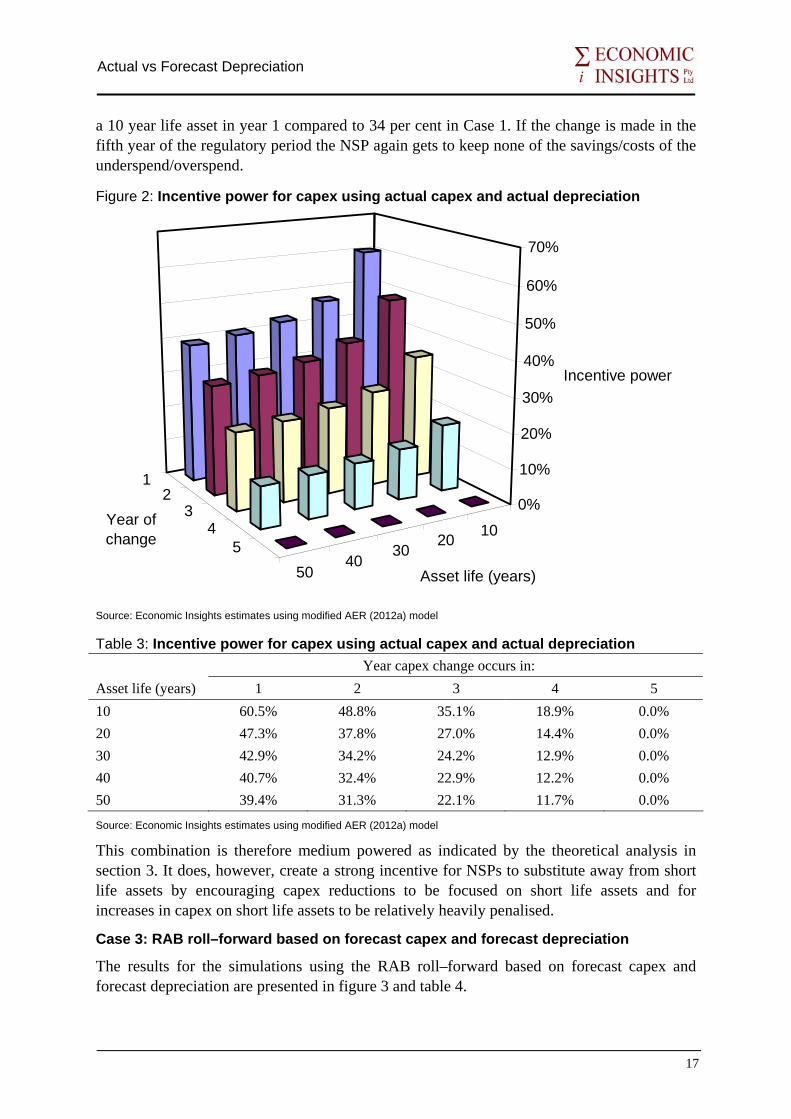
Case 2: RAB roll–forward based on actual capex and actual depreciation
The results for the simulations using the RAB roll–forward based on actual capex and actual depreciation are presented in figure 2 and table 3.
Because actual depreciation is used in the RAB roll–forward, the incentive power results now vary with asset length of life. The incentive power for a change in the first year for an asset with a 50 year length of life (such as poles and wires) is 39 per cent compared to the corresponding incentive power of over 60 per cent for an asset with a 10 year length of life (such as information technology associated with introducing smart networks). There is still a marked difference in incentive powers for a change in the fourth year with an incentive power of 19 per cent for the 10 year life asset and only 12 per cent for the 50 year life asset. This combination, therefore, provides a strong incentive for NSPs to focus capex reductions on short lived assets compared to long lived ones and to correspondingly avoid capex increases on short lived assets. The effect of this will be more pronounced if short and long lived assets are relatively substitutable.
As in Case 1, the incentive power also varies by the year in which the unanticipated capex change occurs. For a 50 year life asset, if the change occurs in the first year of the regulatory period the NSP now gets to keep 39 per cent of the savings/costs of the underspend/overspend compared to 34 per cent in Case 1. The Case 2 result compares with a ‘retention ratio’ of 37 per cent for a similar change in the more complex model used in Economic Insights (2010).
The difference in results between Case 2 and Case 1 are again more pronounced for assets with a short length of life with an incentive power of over 60 per cent for a capex change for
16
Actual vs Forecast Depreciation
a 10 year life asset in year 1 compared to 34 per cent in Case 1. If the change is made in the fifth year of the regulatory period the NSP again gets to keep none of the savings/costs of the underspend/overspend.
Figure 2: Incentive power for capex using actual capex and actual depreciation
102030
4050
12
34
5
0%
10%
20%
30%
40%
50%
60%
70%
Incentive power
Asset life (years)
Year of change
Source: Economic Insights estimates using modified AER (2012a) model
Table 3: Incentive power for capex using actual capex and actual depreciation Year capex change occurs in: Asset life (years) 1 2 3 4 5 10 60.5% 48.8% 35.1% 18.9% 0.0% 20 47.3% 37.8% 27.0% 14.4% 0.0% 30 42.9% 34.2% 24.2% 12.9% 0.0% 40 40.7% 32.4% 22.9% 12.2% 0.0% 50 39.4% 31.3% 22.1% 11.7% 0.0%
Source: Economic Insights estimates using modified AER (2012a) model
This combination is therefore medium powered as indicated by the theoretical analysis in section 3. It does, however, create a strong incentive for NSPs to substitute away from short life assets by encouraging capex reductions to be focused on short life assets and for increases in capex on short life assets to be relatively heavily penalised.
Case 3: RAB roll–forward based on forecast capex and forecast depreciation
The results for the simulations using the RAB roll–forward based on forecast capex and forecast depreciation are presented in figure 3 and table 4.
17

Actual vs Forecast Depreciation
Because both forecast capex and forecast depreciation are now used in the RAB roll–forward, the regulator’s reset of the revenue requirement and correspondingly of allowed maximum revenue are not affected by unanticipated capex changes. As a result, the NSP now gets to keep all of its capex underspend but must correspondingly bear the full cost of any capex overspends. As was the case in Case 1, the incentive power results do not vary with asset length of life. But they also now do not vary with the year in which the unanticipated change occurs. The incentive power for a change in any year for an asset of any length of life is now 100 per cent.
Table 4: Incentive power for capex using forecast capex and forecast depreciation Year capex change occurs in: Asset life (years) 1 2 3 4 5 10 100% 100% 100% 100% 100% 20 100% 100% 100% 100% 100% 30 100% 100% 100% 100% 100% 40 100% 100% 100% 100% 100% 50 100% 100% 100% 100% 100%
Source: Economic Insights estimates using modified AER (2012a) model
Figure 3: Incentive power for capex using forecast capex and forecast depreciation
10203040
50
12
34
5
0%10%20%30%40%50%60%70%
80%
90%
100%
Incentive power
Asset life (years)
Year of change
Source: Economic Insights estimates using modified AER (2012a) model
This combination provides a high powered incentive to reduce capex where possible and to contain capex increases. It does this without creating an incentive to focus reductions (or increases) on any one particular type of asset. It thus does not introduce a distortion between
18
Actual vs Forecast Depreciation
long length of life assets (such as poles and wires) short length of life assets (such as information technology associated with introducing smart networks). It similarly does not encourage NSPs to concentrate capex reductions in the early years of a regulatory period and focus capex increases in the latter years of the period. This Case corresponds to relatively pure incentive regulation based on ex–ante FCM.
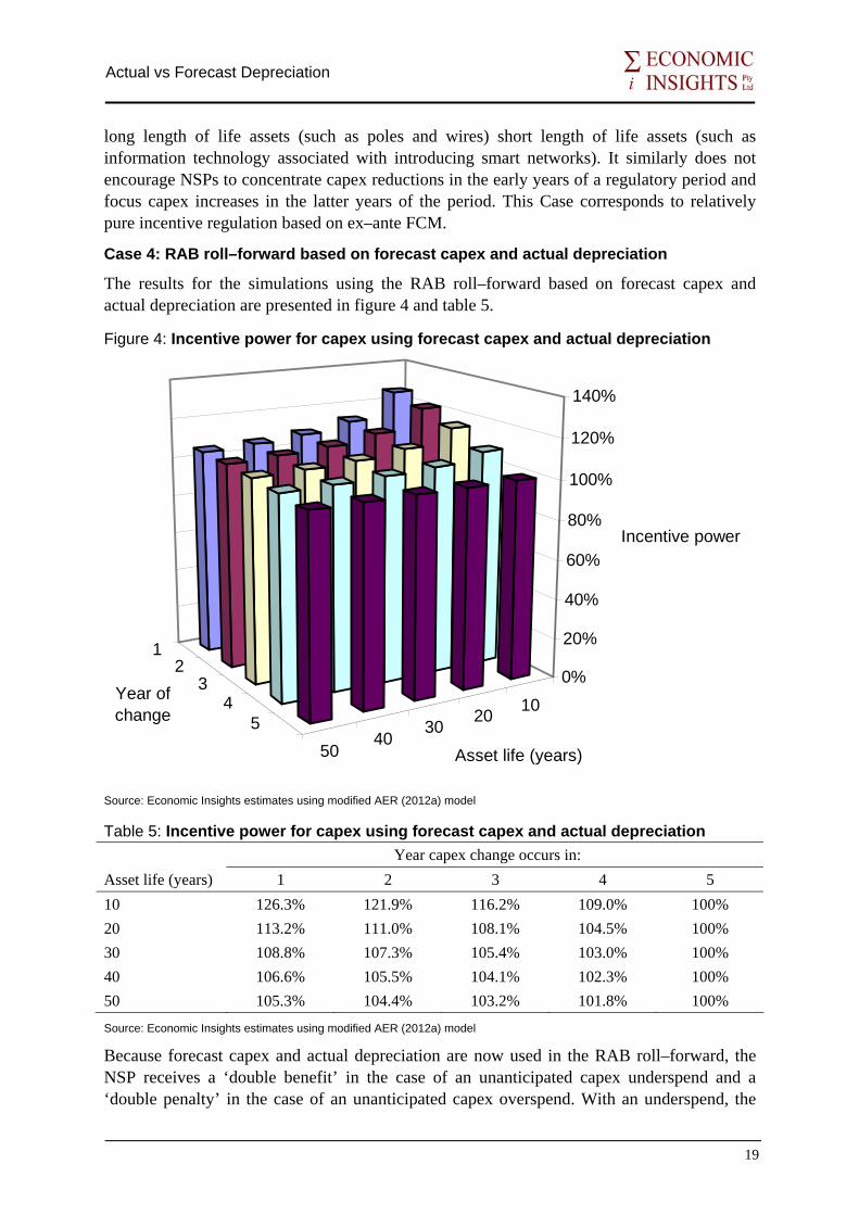
Case 4: RAB roll–forward based on forecast capex and actual depreciation
The results for the simulations using the RAB roll–forward based on forecast capex and actual depreciation are presented in figure 4 and table 5.
Figure 4: Incentive power for capex using forecast capex and actual depreciation
10203040
50
12
34
5
0%
20%
40%
60%
80%
100%
120%
140%
Incentive power
Asset life (years)
Year of change
Source: Economic Insights estimates using modified AER (2012a) model
Table 5: Incentive power for capex using forecast capex and actual depreciation Year capex change occurs in: Asset life (years) 1 2 3 4 5 10 126.3% 121.9% 116.2% 109.0% 100% 20 113.2% 111.0% 108.1% 104.5% 100% 30 108.8% 107.3% 105.4% 103.0% 100% 40 106.6% 105.5% 104.1% 102.3% 100% 50 105.3% 104.4% 103.2% 101.8% 100%
Source: Economic Insights estimates using modified AER (2012a) model
Because forecast capex and actual depreciation are now used in the RAB roll–forward, the NSP receives a ‘double benefit’ in the case of an unanticipated capex underspend and a ‘double penalty’ in the case of an unanticipated capex overspend. With an underspend, the
19
Actual vs Forecast Depreciation
NSP’s RAB is rolled forward on the basis of the higher capex originally anticipated and the lower actual depreciation recognising the underspend. The power of the incentive now exceeds 100 per cent as the NSP is overcompensated for the unanticipated capex reduction. Conversely, in the case of an unanticipated overspend the RAB is rolled forward on the basis of the lower originally anticipated capex and the higher originally anticipated depreciation leading to the NSP being out of pocket by more than the unanticipated capex increase.
As noted in section 3, this combination is essentially an amalgam of Cases 2 and 3 and, consequently, provides excessive incentives for capex reductions and containment of potentially necessary unanticipated capex increases. As with Case 2, it tends to distort investment decisions away from short life assets with a change in capex in year 1 for a 10 year life asset subject to an incentive power of 126 per cent compared to 105 per cent for a corresponding change in a 50 year life asset. As with Case 2, the power of the incentive varies by year, being highest in the first year of the regulatory period and decreasing as the regulatory period progresses. Because this combination provides an excessive incentive to reduce capex and to contain capex increases, it is not considered further.
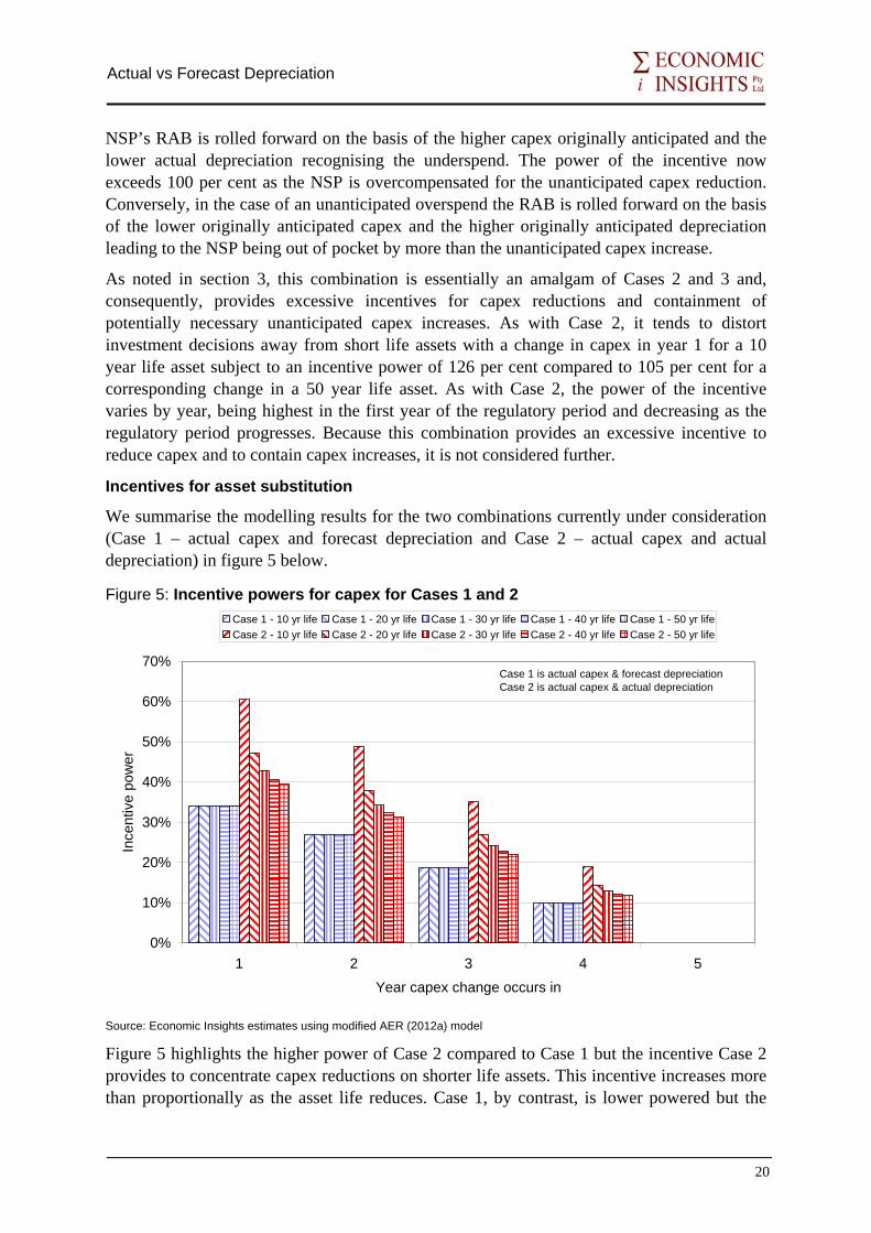
Incentives for asset substitution
We summarise the modelling results for the two combinations currently under consideration (Case 1 – actual capex and forecast depreciation and Case 2 – actual capex and actual depreciation) in figure 5 below.
Figure 5: Incentive powers for capex for Cases 1 and 2
0%
10%
20%
30%
40%
50%
60%
70%
1 2 3 4 5Year capex change occurs in
Ince
ntiv
e po
wer
Case 1 - 10 yr life Case 1 - 20 yr life Case 1 - 30 yr life Case 1 - 40 yr life Case 1 - 50 yr lifeCase 2 - 10 yr life Case 2 - 20 yr life Case 2 - 30 yr life Case 2 - 40 yr life Case 2 - 50 yr life
Case 1 is actual capex & forecast depreciationCase 2 is actual capex & actual depreciation
Source: Economic Insights estimates using modified AER (2012a) model
Figure 5 highlights the higher power of Case 2 compared to Case 1 but the incentive Case 2 provides to concentrate capex reductions on shorter life assets. This incentive increases more than proportionally as the asset life reduces. Case 1, by contrast, is lower powered but the
20

Actual vs Forecast Depreciation
incentive power does not vary with asset life. In both cases there is a higher incentive to defer capex in the early years of the regulatory period compared to the later years (in the absence of an EBSS) and zero incentive in year 5.
It is also useful to compare the above capex incentive powers with the incentive powers for opex reductions. The modified AER (2012a) model returns an incentive power of 100 per cent for a one–off opex reduction in any year of the first regulatory period, in the absence of an EBSS. For a recurrent opex change occurring in the first year of the regulatory period the modified model returns an incentive power of 41 per cent. This is similar in magnitude to the corresponding result presented in Economic Insights (2010) using a more detailed building blocks model. Cases 1 and 2 thus both provide considerably less incentive for a one–off capex change compared to a one–off opex change. The incentive for a one–off capex change in year 1 for medium to long life assets in Case 1 is similar to that for a recurrent change in opex but the incentive for a one–off change in capex for short life assets is considerably higher. For later years of the regulatory period the incentive power for a recurrent opex change is generally higher than that for a one–off capex change, except for the case of short life assets in Case 1 where the incentive is broadly similar.
Summary
The incentive properties of the four cases examined in this section are summarised in table 6.
Table 6: Capex incentives effects
Case 1 2 3 4 Capex Actual Actual Forecast Forecast Depreciation Forecast Actual Forecast Actual Incentive power Low Medium High Excessive Incentive to inflate forecasts Low High Low High Bias against short life assets Low High Low Medium Incentive to defer within period Medium High Low Medium
Cases 1 to 4 have increasing capex incentive powers ranging from low for Case 1 which is equivalent to applying ex–post FCM through to high for Case 3 which is equivalent to applying ex–ante FCM to excessive for Case 4 where the incentive power exceeds 100 per cent. Cases 2 and 4 which use actual depreciation provide NSPs with a high incentive to inflate their capex forecasts compared to Cases 1 and 3 which use forecast capex in the roll–forward. Case 2 provides the largest bias against capex spent on short life assets.
Case 2 also provides the highest incentive to defer capex within the regulatory period with this incentive being highest for short life assets. The effect of introducing an EBSS for capex in all cases would be for the incentive rates applying in the first year of the regulatory period to also apply in the remaining four years of the period. Thus, while introduction of an EBSS would remove the incentive to defer capex within the period, it would not affect the relative incentives to inflate forecasts and relative biases against short life assets.
While Case 2 (actual capex and actual depreciation) provides a medium capex incentive power compared to a lower incentive power for Case 1 (actual capex and forecast
21
Actual vs Forecast Depreciation
depreciation), table 6 highlights the higher incentives Case 2 provides to inflate forecasts, to not invest in shorter life assets and to defer capex within the regulatory period (in the absence of an EBSS) compared to the less distortionary but somewhat lower powered Case 1.
4.2 Incentive power modelling results presented in submissions
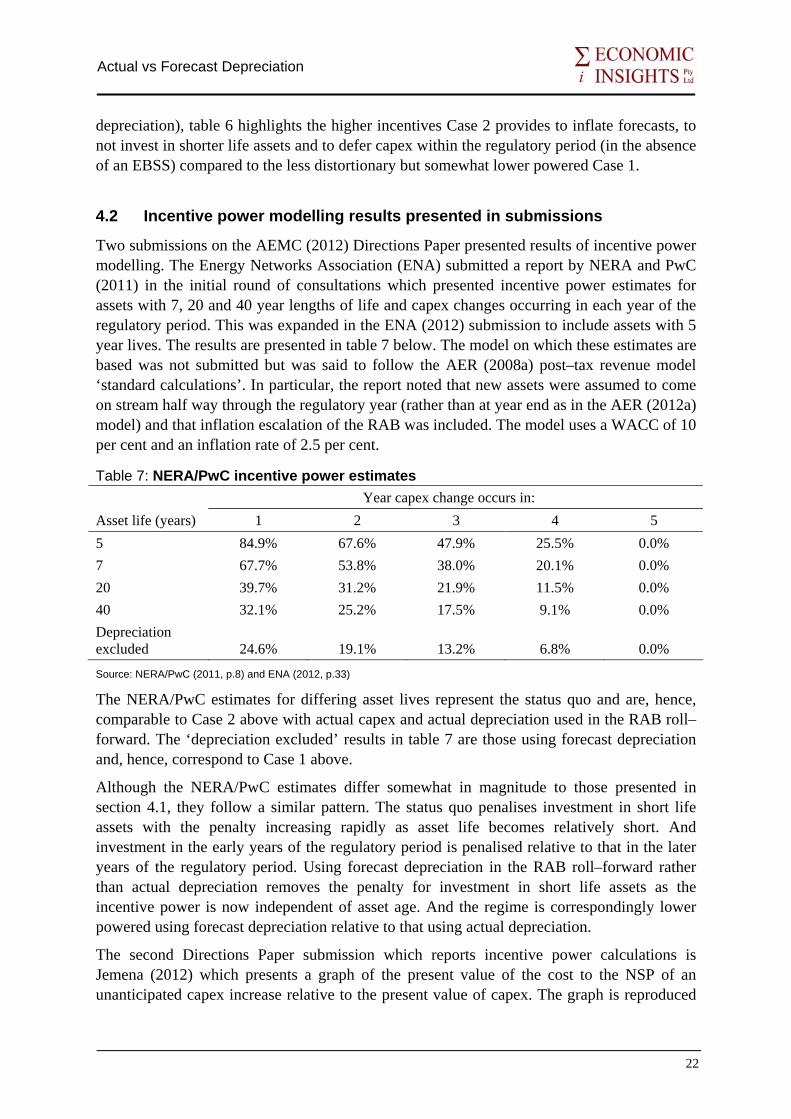
Two submissions on the AEMC (2012) Directions Paper presented results of incentive power modelling. The Energy Networks Association (ENA) submitted a report by NERA and PwC (2011) in the initial round of consultations which presented incentive power estimates for assets with 7, 20 and 40 year lengths of life and capex changes occurring in each year of the regulatory period. This was expanded in the ENA (2012) submission to include assets with 5 year lives. The results are presented in table 7 below. The model on which these estimates are based was not submitted but was said to follow the AER (2008a) post–tax revenue model ‘standard calculations’. In particular, the report noted that new assets were assumed to come on stream half way through the regulatory year (rather than at year end as in the AER (2012a) model) and that inflation escalation of the RAB was included. The model uses a WACC of 10 per cent and an inflation rate of 2.5 per cent.
Table 7: NERA/PwC incentive power estimates Year capex change occurs in: Asset life (years) 1 2 3 4 5 5 84.9% 67.6% 47.9% 25.5% 0.0% 7 67.7% 53.8% 38.0% 20.1% 0.0% 20 39.7% 31.2% 21.9% 11.5% 0.0% 40 32.1% 25.2% 17.5% 9.1% 0.0% Depreciation excluded 24.6% 19.1% 13.2% 6.8% 0.0%
Source: NERA/PwC (2011, p.8) and ENA (2012, p.33)
The NERA/PwC estimates for differing asset lives represent the status quo and are, hence, comparable to Case 2 above with actual capex and actual depreciation used in the RAB roll–forward. The ‘depreciation excluded’ results in table 7 are those using forecast depreciation and, hence, correspond to Case 1 above.
Although the NERA/PwC estimates differ somewhat in magnitude to those presented in section 4.1, they follow a similar pattern. The status quo penalises investment in short life assets with the penalty increasing rapidly as asset life becomes relatively short. And investment in the early years of the regulatory period is penalised relative to that in the later years of the regulatory period. Using forecast depreciation in the RAB roll–forward rather than actual depreciation removes the penalty for investment in short life assets as the incentive power is now independent of asset age. And the regime is correspondingly lower powered using forecast depreciation relative to that using actual depreciation.
The second Directions Paper submission which reports incentive power calculations is Jemena (2012) which presents a graph of the present value of the cost to the NSP of an unanticipated capex increase relative to the present value of capex. The graph is reproduced
22
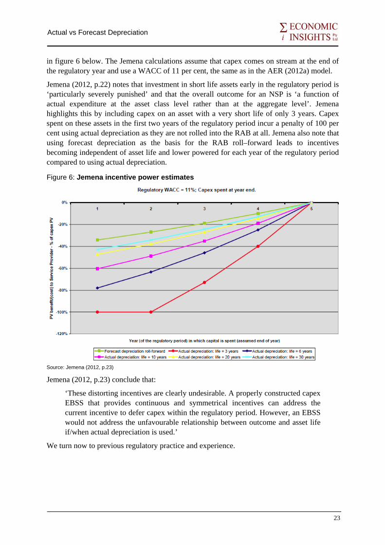
Actual vs Forecast Depreciation
in figure 6 below. The Jemena calculations assume that capex comes on stream at the end of the regulatory year and use a WACC of 11 per cent, the same as in the AER (2012a) model.
Jemena (2012, p.22) notes that investment in short life assets early in the regulatory period is ‘particularly severely punished’ and that the overall outcome for an NSP is ‘a function of actual expenditure at the asset class level rather than at the aggregate level’. Jemena highlights this by including capex on an asset with a very short life of only 3 years. Capex spent on these assets in the first two years of the regulatory period incur a penalty of 100 per cent using actual depreciation as they are not rolled into the RAB at all. Jemena also note that using forecast depreciation as the basis for the RAB roll–forward leads to incentives becoming independent of asset life and lower powered for each year of the regulatory period compared to using actual depreciation.
Figure 6: Jemena incentive power estimates
Source: Jemena (2012, p.23)
Jemena (2012, p.23) conclude that:
‘These distorting incentives are clearly undesirable. A properly constructed capex EBSS that provides continuous and symmetrical incentives can address the current incentive to defer capex within the regulatory period. However, an EBSS would not address the unfavourable relationship between outcome and asset life if/when actual depreciation is used.’
We turn now to previous regulatory practice and experience.
23
Actual vs Forecast Depreciation
5 RECENT REGULATORY PRACTICE AND EXPERIENCE
5.1 Australian Energy Regulator
The AER has now undertaken electricity transmission revenue reviews for TNSPs in Victoria, South Australia, NSW, Tasmania and Queensland. As required under Chapter 6A of the NER, actual depreciation has been used in the RAB roll–forward in these reviews.
In 2008 the AER released its final report on the RAB roll–forward model (RFM) it proposed to use in electricity distribution price reviews. AER (2008b, pp.5–6) noted:
‘The AER considers clause S6.2.1(e)(5) of the NER provides for the possibility of actual and forecast depreciation to be part of the capex incentive framework. … The use of forecast depreciation involves using the amount of depreciation specified in the regulatory determination (which is based on forecast capex and forecast inflation) and adjusting this for actual inflation during the relevant regulatory control period. The RFM does not accommodate this approach … The AER notes the general support for utilising actual depreciation in the RFM and has maintained this in the final model. The AER will further consider views … having regard to any specific circumstances raised, during the process of making a distribution determination for each DNSP.’
In practice the AER has used actual depreciation in the RAB roll–forward in all its electricity distribution reviews to date. In its review of the Victorian DNSPs, AER (2010, p.461) stated its views on the need to have strong capex incentives in place as follows:
‘the AER’s view is that the incentive framework which applies to forecast capex under Chapter 6 is relatively weak and the general incentives on capex and opex are unbalanced, particularly under the arrangements put in place by the ESCV where depreciation does not form part of the incentive framework…. the AER is of the view that it is required to provide effective incentives or to strengthen the incentives for Victorian DNSPs to seek out efficiencies wherever possible in its capex programs.’
In the context of the choice between actual and forecast (or ‘regulatory’) depreciation, AER (2010, p.462) also noted the objective of achieving consistency of treatment as follows:
‘Clause 6.12.1(18) of the NER provides the AER with discretion on whether depreciation for establishing the RAB is to be based on actual or forecast capital expenditure. While the AER does not view consistency as an end itself, it is an underlying rationale for the establishment of national regulatory arrangements, and as noted above, its view on the desirability of the use of actual depreciation reflects that capex incentives are relatively weak if depreciation is not included in the incentive framework.’
The AER also noted concerns expressed by the Victorian Minister for Energy and Resources and the Victorian Department of Primary Industries (DPI) that the Victorian DNSPs had previously underspent their regulatory capex allowances. The AER observed that the main
24
Actual vs Forecast Depreciation
period of capex underspend had occurred at the same time that a capex EBSS applied in Victoria. AER (2010, p.462) went on to note that ‘the revealed cost approach, whereby actual expenditures provide a good indicator of efficient costs in the future, relies on an effective incentive framework’. The Victorian Minister subsequently appealed the AER’s decision to use actual rather than forecast capex in the RAB roll–forward but the appeal was rejected by the Australian Competition Tribunal as it considered the AER had followed required procedures in reaching its decision. This will be covered further later in this section.
In its submission in response to the AEMC Directions Paper, AER (2012b, p.24) argued that it should have ‘the flexibility to adopt either a high powered or a lower powered depreciation incentive for TNSPs to achieve a balanced capex incentive framework, consistent with the approach currently allowed for DNSPs under chapter 6’.
In the case of gas distribution NSPs, the National Gas Rules (NGR) also provide for a choice to be made between the use of actual and forecast depreciation in rolling forward the RAB to the start of the next regulatory period (Division 6, Clause 90(2)). However, in its gas DNSP decisions to date, the AER has chosen to use forecast depreciation rather than actual depreciation as it has done in the case of electricity DNSPs. AER (2011b, p.27) noted:
‘The AER’s primary reasons for deciding on a forecast depreciation approach included the dynamics of the gas industry (including a gas distributor’s ability to defer investment), the service quality incentives facing gas distributors and consistency with other gas access arrangements.’
AER (2011a, pp.47–8) earlier explained the difference in approaches adopted for electricity and gas distribution NSPs as follows:
‘An actual depreciation approach is typically used for electricity distribution. The AER considers that the actual depreciation approach is appropriate for electricity distribution given the dynamics of that industry and the service quality incentives facing those businesses. Electricity distributors generally operate in a relatively more dynamic environment than gas distributors, where growing demand can apply significant pressure to increase spending. In such circumstances, the AER is concerned that such spending be efficient, while deferral of expenditure is relatively less likely given the pressing demands. To prevent electricity distributors compromising on service quality, service quality incentive schemes exist that penalise poor performance. In contrast, gas distributors generally operate in a less dynamic market, which can give them scope to defer expenditure as the situation allows. Gas distributors are also not subject to any service quality incentive scheme.’
AER (2011b, p.27) expanded on the AER’s concerns regarding what it saw as greater scope for capex deferral in gas distribution as follows:
‘In electricity distribution, service can be completely cut by relatively minor equipment failures. However, gas service is unlikely to be interrupted through an increase in UAG [unaccounted for gas], unless a major breach occurs. This provides gas distributors with relatively greater flexibility in the timing of replacement capex than electricity distributors.’
25
Actual vs Forecast Depreciation
The AER also noted that forecast depreciation has been used in all gas distribution access arrangements to date and it considered this to be a relevant consideration in arriving at the preferred approach.
In response to NSP concerns that the use of forecast depreciation could lead to some rolled forward asset values becoming negative, AER (2011b, p.28) observed:
‘The AER considers the possible occurrence of a negative asset value at the end of the access arrangement period for one or more asset classes does not invalidate a forecast depreciation approach. … Negative asset values will only emerge in the present context in circumstances where Envestra received a forecast depreciation allowance which subsequently proves to be greater than the capex Envestra actually spent on the assets in question. While this is an unlikely outcome, it could occur. If it does occur the negative asset value represents funds received from tariff revenues for which no costs were incurred. This money should then be returned to customers as a negative asset. Thus the overall effect is neutral for both Envestra and its customers.’
5.2 IPART
The NSW regulator, IPART, currently uses the building blocks model to regulate the prices of water services (metropolitan water and bulk water) and passenger transport services (rail and buses). Until energy network regulation was transferred to the AER, IPART also regulated NSW electricity and gas distribution NSPs using the building blocks model.
IPART may use either actual or forecast depreciation in the RAB roll forward, but since 2004 it has usually used forecast rather than actual depreciation (IPART 2009, p.9). Its decision to use forecast depreciation in the RAB roll–forward in its 2004 electricity distribution determination was made in the context of NSW DNSPs having overspent their capex allowances during the previous regulatory period. IPART (2004, p.209) stated:
‘The Tribunal is concerned about providing a regulatory framework that is transparent and limits uncertainty for DNSPs. It has therefore decided to allow DNSPs to recover foregone depreciation on the capital overspend – that is, to conduct the roll forward of the RAB on the basis of regulatory rather than actual depreciation.
‘The Tribunal’s decision means that when the RAB is rolled forward at future regulatory resets it will be on the basis of regulatory rather than actual depreciation, regardless of whether actual capital expenditure is higher or lower than regulatory allowances.’
IPART also decided not to alter the 1998 opening RAB or alter the depreciation profile of assets implying that the difference between forecast and actual depreciation in the previous regulatory period would be a one-off gain (or loss if it is negative) to the firm.
Some years earlier, IPART (1999) had consulted on whether to use of forecast or actual capex in the roll–forward, but did not explicitly discuss the use of forecast or actual depreciation. IPART also considered the option of reversing the RAB adjustment at the end
26
Actual vs Forecast Depreciation
of the next period. Thus, in the roll–forward the NSP would receive as a benefit, the difference between forecast and actual capex, but the corresponding adjustment made in the previous period would be reversed (IPART 1999, p.23).
5.3 Essential Services Commission
In its 2005 electricity distribution price review for the regulatory period 2006–10, the Essential Services Commission (ESC) used the roll–forward formula specified in the Victorian Tariff Order. The ESC (2005b, p.323) applied the following formula with all quantities expressed in real dollars:
There was no capex prudency test because the ESC (2005a, p.278) preferred to ‘rely on the incentive properties of the price capping regime’. Where actual data was not available the ESC used estimates from the previous review, consistent with the method detailed in the NER. The resulting asset value series (in real terms) was then adjusted to current prices using the CPI. The Victorian Tariff Order did not provide for the revaluing of existing assets.
ESC (2005b, p.268) expressed concern about the information asymmetry faced by the regulator when it came to capex and the incentive for NSPs to underspend their capex allowances as follows:
‘The balance between overcompensating and undercompensating the distributors for their expenditure requirements is made more complex for the regulator given the information asymmetry that exists between the regulator and the distributors. Investment in the distribution network involves a large number of relatively small projects. This contrasts with investment in the transmission network which involves a small number of relatively large projects, which may more readily be assessed on a project–by–project basis.
As demonstrated in this price review, when requested to provide supporting information, the distributors are able to produce a large amount of material to support individual projects. However, this material does not constitute a commitment to execute those projects nor an assessment of their capacity to execute them within the regulatory period. This requires that the distributors’ proposals for future expenditure must be subject to careful scrutiny.
However, the Commission does not have the information necessary to develop the counterfactual at this project by project level.’
These concerns and the associated case for using forecast depreciation in the RAB roll–forward were further stated by DPI (2012, pp.9–10) in its submission on the AEMC Directions Paper:
‘The privately owned Victorian businesses have strong incentives to over–forecast capex to secure higher regulatory allowances. … Regulatory depreciation has a disincentive effect on over–forecasting capex. If capex is consistently over–
27
Actual vs Forecast Depreciation
forecast under a regulatory depreciation regime, the RAB will be written down more quickly than indicated by the physical assets. At this extreme, the RAB could be written down to a very low value which would decrease the business’s building block revenue (the return on assets and depreciation would be based on a smaller asset base) and could therefore have an impact on the business’s cash flow position.’
In its final Gas Access Arrangement Review, ESC (2008, p.425) calculated the RAB roll–forward to the start of the new regulatory period in accordance with s.8.9 of the Gas Code. The opening RAB at the commencement of previous regulatory period was updated for actual net capex (excluding capital contributions and disposals) deducting forecast/regulatory depreciation. ESC (2008, pp.435–6) noted:
‘the Commission’s approach … was to infer that distributors take the assumed regulatory depreciation amount as a return of capital, irrespective of actual capital expenditure in the 2003 to 2007 period.
‘No comments were received on this approach in response to the draft decision and the Commission has maintained this approach in this final decision.’
5.4 Victorian Minister’s Appeal
In February 2011 the Victorian Minister for Energy and Resources appealed against some aspects of the AER (2010) electricity distribution price review for Victoria. One aspect was the AER’s use of actual rather than forecast depreciation in the RAB roll–forward, contrary to the approach adopted by the ESC (2005b) in the previous review and contrary to the Minister’s submissions to the AER.
The Minister (2011a,b) argued in the appeal that the AER had placed too much weight on achieving jurisdictional consistency without adequately recognising the different circumstances applying in Victoria. In particular, the Minister argued that privately–owned NSPs in Victoria had a history of underspending capex and would have more incentive to over-inflate their capex forecasts if actual depreciation were used compared to some other jurisdictions where largely government–owned NSPs had a history of overspending capex and were likely to be less responsive to financial incentives. The Minister also noted that Victorian consumers had already paid for regulatory depreciation in the previous period and would effectively be paying twice if actual depreciation were then adopted.
The Minister also questioned the accuracy of what he saw as the AER’s implication that previous capex underspends in Victoria resulted from the capex EBSS then applying and that stronger incentives were necessary if revealed costs were to provide a good indicator of future efficient costs. The Minister argued revealed costs were more relevant for forecast efficient opex but capex requirements will change due to external drivers such as changes in peak demand.
The Minister argued the effective constraint on over–inflating capex forecasts which the use of forecast depreciation provides is consistent with the NEO, in particular the promotion of ‘efficient investment in, and efficient operation and use of, electricity services for the long term interests of consumers of electricity with respect to … price’.
28
Actual vs Forecast Depreciation
The Australian Competition Tribunal (2012, para 336)) rejected the Minister’s appeal as follows:
‘In our judgment, the Minister has fallen well short of demonstrating either of the grounds of review upon which he relied. The AER applied the appropriate principles and the decision to which it came was perfectly open to it on the material before it. The mere fact that it may also have been open to the AER to choose the other available option does not render the choice which it actually made erroneous.’
That is, being a judicial review body, the Tribunal considered the AER had followed required procedures in reaching its decision.
5.5 United Kingdom
The UK has had a varied practice in relation to the calculation of the regulatory asset base (referred to as the ‘RAV’ by Ofgem and ‘RCV’ by Ofwat), largely because many of the regulated businesses were privatised before the regulatory framework was introduced and the initial regulatory capital base was calculated from market values. Certain legacy arrangements have influenced depreciation levels and regulators have allowed depreciation profiles to adjust to industry cash–flow needs.
Electricity
The approach to calculating the RAV adopted by Ofgem, the UK energy regulator, has differed in several key respects to the approach to calculating the RAB for building blocks regulation in Australia. And the UK approach is currently undergoing a major revision as part of the move to the RIIO (Revenue = Incentives + Innovation + Outputs) regulation model.
In the past Ofgem has rolled–forward the opening RAV for new regulatory periods on the basis of actual capex and actual depreciation but all capex has been lumped together and been subject to an accelerated regulatory depreciation rate of 20 per cent. When asked by Economic Insights whether the use of actual depreciation had created incentives to reduce capex on short life assets relative to long life assets, Ofgem replied that its use of a weighted average asset life for all capex for depreciation purposes removed the incentive that would otherwise exist.
Ex–ante allowances have been set on the basis of forecasts at the beginning of the price control and Ofgem has used a sharing factor to split the benefits or the costs of the difference from forecast to actual between consumers and the NSP. Up until 2010 Ofgem applied all of costs and benefits of variations from the opex allowance to the NSP and shared capex variation costs using a ‘roller’ mechanism which rolled up gains and losses during one price control and trued them up in the next.
Ofgem is currently undertaking a review of electricity transmission price controls for an eight–year period from 1 April 2013 to 31 March 2021. This will be the first transmission price control to reflect the new RIIO regulatory model. An important change in this review will be the adoption of an economic asset life for all new capex of 45 years. The accelerated depreciation life of 20 years will remain in place for existing assets and some renewable
29
Actual vs Forecast Depreciation
energy related capex already commenced. Ofgem (2011a, p.47) noted that it has allowed for the expected increasing importance of shorter asset lives in choosing the 45 year figure as follows:
‘We have taken into account several factors in determining the appropriate economic asset life. These include … the technical life of the assets (54–60 years), which were not disputed by companies, and the clear expectation of increased electricity usage in the plausible scenarios of future energy demand. In determining the economic asset life we have also allowed for a reasonable increase in shorter life assets as networks become smarter and for some early retirement of assets as generation locations change.’
Ofgem has provided incentives for NSPs to reduce their capex and to contain their forecast capex for the next regulatory period. An incentive rate has been applied to individual NSPs under Ofgem’s Information Quality Incentive (IQI) scheme under which NSPs are presented a menu of choices from which they can nominate their capex forecast. The lower the NSP’s capex forecast is compared to Ofgem’s baseline, the higher the incentive rate that applies. The aim is to structure choices so that NSPs achieve the best result by putting in their most accurate forecast of achievable expenditure.
The bounds of the incentive rate have been set to provide sufficient incentive at the lower end for NSPs not to spend unnecessarily and with regard to risks faced by the NSPs and the risk of windfall profits at the upper end.
In its fifth electricity distribution price control review in 2010 Ofgem made a further significant change in its incentive regime. In an effort to equalise incentives applying to opex and capex, Ofgem now takes a set percentage of ‘totex’ (total expenditure comprising opex plus capex less some minor exemptions) as the RAV addition while the balance of totex is allowed to be expensed in the year it is incurred (ie treated as opex). Ofgem (2011b, p.57) indicated the capex–equivalent percentage would be set as follows:
‘The percentage that we will add to the RAV will be set at the price control review to strike a fair balance between existing and future consumers, in light of the proportion of capex–like costs expected during the price control period. Our approach will be consistent with our objective to equalise incentives between opex and capex in the overall control.’
Ofgem (2011b, p.59) goes on to explain the capex incentive regime as follows:
‘The calculation of the net additions to the RAV will reflect two parameters which will be set at the price control review:
• first, the efficiency incentive rate. The higher the efficiency incentive rate, the smaller the proportion of any overspend that is passed on to consumers, including through net additions to the RAV
• second, the fixed percentage of totex to be added to the RAV. This … effectively determines the extent to which adjustments made in light of actual totex are split between fast and slow money.’
30
Actual vs Forecast Depreciation
The other important change Ofgem is implementing as part of the RIIO process is an annual updating of the RAV for reporting purposes and to form the basis for the opening RAV in the next regulatory period. Ofgem (2011b, p.118) describes this process as follows:
‘At the end of each year of a price control, we will publish an indicative updated RAV for each network company with a view to confirming the effective RAV at the end of the period (March 2021). In ascertaining these values it is important that the treatment of expenditure that network companies incur in this period is consistent with the principles and specific issues set out in the final proposals – that is, the same constituents of costs are added to the RAV (ie as the slow money). We add all costs on a normal accruals basis.’
Ofgem indicated it saw this process as a means of reducing uncertainty for NSPs regarding what the allowed opening RAB for the next regulatory period would be. Ofgem will also be truing up totex variations from allowances on a rolling, two years in arrears basis, rather than during the subsequent price control.
Water
Ofwat uses an RCV roll–forward method in which:
‘Capital expenditure to enhance and maintain the network, which is assumed in setting price limits, is added to the RCV. Any capital grants or contributions towards the cost of the new assets are deducted. Current cost depreciation (based on the MEA value of the assets), which is assumed in setting price limits, is deducted from the RCV each year.’ (Ofwat 2010, p.2).
This suggests that forecast depreciation is used in the roll–forward. The method differs from Australian regulatory treatment because capex is separated into two components. Capex to maintain and replace infrastructure assets (infrastructure renewals expenditure) is not directly added to the RCV. Rather, it is compared with the infrastructure renewals charge (IRC), and the difference is added to or deducted from the RCV each year.
This reflects the extent to which more (or less) money has been spent on maintaining the infrastructure asset base than assumed in price limits, thus increasing (or decreasing) the value of the capital base to be remunerated.
There are other elements to the RCV roll–forward including ‘logging up/down’ and output shortfalls. When there are changes to specific legal obligations placed on a regulated business since the price limits were last set – and there has been no interim determination to pass these costs through – the RCV may be ‘logged up’ to reflect the reasonable net additional costs. Where a company has failed to meet the outputs required and allowed for in the previous review, the RCV is also reduced to take account of such ‘shortfalls’.
Ofwat (2010, p.4) has recently introduced capex incentives as follows:
‘At the 2009 price review, we introduced the capital expenditure incentive scheme (CIS). It provides strong incentives for the companies to put forward challenging and efficient business plans and to strive to beat our price limit assumptions after them.
31
Actual vs Forecast Depreciation
‘Under the CIS, each company recovers its actual capital expenditure plus or minus an incentive allowance that depends on its forecast of capital expenditure and its actual expenditure in 2010–15. At the next price review, we will reconcile the rewards or penalties due under CIS, taking account of actual capital expenditure along with the expenditure assumptions and additional income allowed in price limits. We will also adjust each company’s regulatory capital value (RCV) to reflect actual 2010–15 capital expenditure.’
5.6 United States
In the USA, each time a rate case is conducted, the asset base is assessed in order to determine a fair return on the investment by the utility. Assets are valued at historical cost net book value and depreciation is calculated accordingly. Hence, a version of actual depreciation is used in the roll–forward. However, the rate base is subject to two tests:
• Capex that has been undertaken is subject to a prudency test. For each investment, the test is whether a reasonable person would have undertaken that investment with the information available at the time. This avoids consumers paying for unwise or extravagant investments.
• Assets are subject to a ‘used and required to be used’ test. This tests whether an asset is no longer in service or contributing to the operating capacity of the business. Such assets are considered redundant and are ‘written off’ in the rate base.
5.7 New Zealand
Around 60 per cent of New Zealand energy distribution NSPs are currently subject to default CPI–X price path regulation based on projected productivity and input price growth for the relevant distribution industry relative to the economy as a whole. The regulator is the Commerce Commission. The other 40 per cent of NSPs are exempt from regulation. Under changes made to the Commerce Act in 2008, regulated NSPs can apply to move from the default price path to a customised price path. In submitting such an application, the NSP must undertake a building blocks calculation. Before this process becomes operational, the Commerce Commission is required to develop ‘input methodologies’ that specify how a building blocks review would be undertaken and the information required.
Commerce Commission (2010) presented the proposed methodologies to be used but these are currently subject to appeal. The input methodologies report’s treatment of the depreciation component of the RAB concentrated on the depreciation method and asset lives to be considered. New Zealand operates a well established Information Disclosure Data reporting regime for all energy NSPs and this would form the basis of information used to update the RAB from year to year for all NSPs (both regulated and exempt). Annual updating of the RAB for reporting purposes would therefore be on the basis of actual capex and actual depreciation. Similarly, the opening RAB for each regulatory period for NSPs subject to ongoing building blocks regulation would be the NSP’s Information Disclosure Data RAB and, hence, the roll–forward would effectively be based on actual capex and actual
32
Actual vs Forecast Depreciation
depreciation. It is important to note, however, that the building blocks method has not as yet been applied to the regulation of an energy NSP in New Zealand.
5.8 Summary
Australian regulatory practice with regard to the use of actual or forecast depreciation in the RAB roll–forward has varied across jurisdictions and within jurisdictions, even at the same time. The two largest States have used and advocated the use of forecast depreciation although their stated reasons have differed somewhat. Victoria has been mainly concerned with the incentive that actual depreciation would give its privately–owned NSPs to underspend capex and exploit information asymmetries in inflating capex forecasts that the regulator would then find difficult to adequately assess. New South Wales, on the other hand, has favoured forecast depreciation as a means of providing a higher level of certainty to its government–owned NSPs which have generally overspent their capex allowances in recent years.
At the federal level, the AER has favoured the use of actual depreciation for electricity distribution NSPs to provide consistency with the mandated use of actual depreciation for electricity transmission NSPs, to address what it sees as an imbalance with opex incentives and because it believes there is less scope for electricity distribution NSPs to defer capex in a growing and dynamic market (AER 2011a, pp.47–8). However, in the case of gas distribution NSPs, the AER has used forecast depreciation in the RAB roll–forward because it believes the nature of gas distribution provides greater scope for NSPs to defer capex without obvious immediate adverse consequences for customers compared to electricity distribution and given the absence of a countervailing service quality incentive scheme for gas distribution NSPs.
The use of actual depreciation in the RAB roll–forward has been the norm in the overseas jurisdictions examined although this has occurred in different circumstances to those found in Australia. In the UK Ofgem has used actual depreciation but has also used a common length of life assumption for all capex, the effect of which has been to reduce the bias against capex on short life assets which would otherwise exist. In the US rate of return regulation based on historic net book value has been used but with capex included being subject to ex–post prudency and used and useful tests.
New Zealand plans to use actual capex in the RAB roll–forward (should building blocks customised price paths be implemented) but this is closely linked to its longer history of mandating annual information disclosure data for all NSPs and the fact that only some NSPs are subject to price controls. Ofgem in the UK is also moving to annual updating of the RAB using actual depreciation as a means, among other things, of reducing uncertainty for NSPs.
The review of recent regulatory practice highlights the importance of jurisdiction–specific circumstances in the choice of using actual or forecast depreciation in the RAB roll–forward. It has not been a case of ‘one size fits all’ and the approach used in each jurisdiction reflects the relative issues and concerns that have evolved in that jurisdiction. None of the regulatory regimes examined are without a number of shortcomings.
33
Actual vs Forecast Depreciation
6 STAKEHOLDERS’ VIEWS
Support for discretion
Submissions to the AEMC on its Directions Paper generally supported the AER’s proposed rule change regarding the use of actual or forecast depreciation in the RAB roll–forward. For example, CitiPower/Powercor/ETSA Utilities (2012, p.30) stated:
‘the Businesses strongly support the Rules providing for discretion on the part of the AER to apply forecast or actual depreciation.’
DPI (2012, p.10) noted the importance of the AER having discretion as follows:
‘The Victorian Government strongly supports the use of forecast depreciation for the Victorian DNSPs to appropriately balance the capex efficiency incentive to not over–forecast capex as part of the regulatory determination process. However, the Victorian Government recognizes that actual depreciation may be more appropriate with the circumstances that apply in other jurisdictions. The AER therefore requires the discretion to use either forecast depreciation or actual depreciation, depending on the circumstances.’
And Jemena (2012, p.24) stated its support for discretion as follows:
‘Jemena supports a change to the rules to give the AER guided discretion to choose between using forecast and actual deprecation in the roll-forward calculation but with a presumption in favour of using forecast depreciation if there is a capex EBSS.
However, while nearly all stakeholders supported the AER having discretion, some expressed a strong view as to which of actual or forecast depreciation was appropriate. For instance, SP AusNet (2012, p.4) observed:
‘There is no reasonable justification for allowing actual depreciation as an option in the regulatory regime’.
Balance of incentives
While many submissions acknowledged that there is currently an imbalance in incentives between opex and capex, views differed on what an appropriate response to this would be. For example, CitiPower/Powercor/ETSA Utilities (2012, p.30) supported the use of actual capex in providing a better balance of incentives:
‘where no EBSS is applied to capex but is applied to opex …the efficiency incentives will be imbalanced. This imbalance in the efficiency incentives for opex and capex can be mitigated by the use of an actual depreciation approach in preference to a forecast depreciation approach. This is because … the use of an actual depreciation approach creates additional capex efficiency incentives not present under a forecast depreciation approach.’
However, other submissions noted that the introduction of an EBSS for capex was the first best response to current imbalances. Grid Australia (2012, p.8) noted:
34
Actual vs Forecast Depreciation
‘A well designed capital expenditure incentive scheme should be the first preference to providing capital expenditure incentives. Grid Australia considers that this is best achieved by applying an EBSS to capital expenditure and requiring that the AER apply forecast depreciation to the roll–forward of the RAB.’
Similarly, the ENA (2012, p.34) stated:
‘ENA reiterates its support for the application of the EBSS to capital expenditure as the preferred approach to providing well calibrated incentives.’
In a report prepared for the ENA, NERA/PwC (2012, p.v) argued the use of actual depreciation was very much a second best approach:
‘we considered the application of actual depreciation to be a second best approach to providing strengthened incentives for capital expenditure efficiency. Moreover, given the perverse incentives that the use of actual depreciation may create, its use may not be appropriate even if an EBSS for capital expenditure is not introduced.’
Inflation of capex forecasts
Views differed on whether the use of actual depreciation would provide an incentive for NSPs to over–inflate their capex forecasts and, if so, whether this was a readily manageable problem. DPI (2012, p.8) thought this was a potentially significant problem that would be hard to manage;
‘The Victoria Government is concerned that any capital expenditure incentive benefits associated with applying actual depreciation are likely to be more than offset by the privately–owned Victorian businesses over–forecasting their capital expenditure requirements for the next regulatory control period and obtaining higher regulatory allowances (such as allowed costs of financing higher forecast capex).
‘The AER is subject to information asymmetries …’.
DPI went on to quote the ESC’s experience and the difficulty it had encountered in trying to assess the relative large number of capex projects a distribution NSP is able to put forward as being justifiable.
Some of the NSPs argued that the AER should be able to readily manage the problem. CitiPower/Powercor/ETSA Utilities (2012, p.29), for instance, argued:
‘The AER has the power to reject a DNSP's forecast capex where it does not reasonably reflect the capex criteria and substitute forecasts that reflect those criteria. Indeed, the Businesses observe that the AER has substituted its own forecast capex in every distribution and transmission determination under the Rules to date.’
The AER (2012b, p.4) was relatively sanguine about the problems it faces:
35
Actual vs Forecast Depreciation
‘While it is not possible to precisely identify the extent to which the use of actual depreciation reinforces the incentive for a NSP to overstate its forecast capex requirements, the AER considers that:
• as previously discussed, there is always an incentive for an NSP to overstate its forecast capex. This is irrespective of the depreciation method adopted
• the issue of incentives for an NSP to overstate its forecast should be addressed separately
• to the extent that an NSP responds to the incentives where actual depreciation is adopted, the AER will be able to have regard to past expenditure out-turns in setting an NSP's forecast capex allowance.’
Asset length of life distortions
Nearly all NSPs making submissions on the Directions Paper noted that the use of actual depreciation creates a disincentive to undertake capex on short life assets. In the case of transmission, Grid Australia (2012, p.8) argued:
‘applying actual depreciation as an incentive mechanism delivers a disproportionally large incentive against additional expenditure on short lived assets. … Smart network technologies are expected to increasingly be used for the delivery of network services over the coming years. Given many of the innovative technologies associated with smart networks would be expected to have relatively short economic lives compared to traditional network assets, the application of actual depreciation may create disincentives for NSPs to implement these technologies. Efficient transmission services already rely heavily on investment in short lived assets such as protection, control and communications systems. Requiring forecast depreciation to be applied overcomes this issue and avoids this potential bias.’
Similarly, in the case of distribution the ENA (2012, p.33) notes:
‘the penalty from spending more on assets with a short economic life is inappropriately large compared to longer lived assets. This is because the “penalty” from one extra unit of expenditure increases as the asset age falls.
‘The impact of this penalty is to create a relative disincentive for NSPs to incur additional expenditure on assets with a short economic life relative to those with a longer economic life. This incentive particularly affects investments in IT infrastructure and other ‘smarter’ technologies; which would be expected to become more pronounced in future years given the developments of smart meters and smart grids. While these assets may make up only a small proportion of the total asset base for an NSP, they have the capability of being used as a substitute for longer lived network assets, or at least provide an NSP with additional information that allows it to make a better decision about when network augmentation or asset replacement is required. It follows that the application of actual depreciation is likely to lead [to] sub–optimal investments in innovative
36
Actual vs Forecast Depreciation
technologies and potentially an increased reliance on network solutions with a long asset life.’
SP AusNet (2012, pp.4–5) expanded on the problems it saw with the AER’s current practice of using actual depreciation as follows:
‘In practice, SP AusNet has found that the incentive regime distorts the investment decision process in extreme ways.
The IT allowance provided for under the Rules is a maintain case only, therefore, any increase in IT expenditure to materially increase functionality or introduce new functionality can only be justified by savings generated to capital or operating costs or benefits from service standard improvements. However, the assessment of such expenditure starts with a massive disadvantage when being ranked against alternative investment opportunities, particularly at the start of a regulatory period.
For example, in the first year of SP AusNet’s current electricity distribution regulatory control period a $10M IT project will need to generate an NPV efficiency/service standard benefit of around $8.5M before it becomes NPV positive on a stand alone basis whereas a $10M network investment need only generate a NPV saving of $3M. Therefore, all things being equal, IT projects are artificially pushed down the priority list of capex projects in the investment optimisation processes. Given many of these projects would generate net benefits for customers, the current approach detracts from the achievement of the NEO.
This is particularly perverse given that potential solutions to mitigate future network costs require substantial investments in IT systems (for example, dynamic monitoring, selfhealing networks, smart meter enabled TOU [time–of–use] tariffs and DSM [demand–side management] to address peaky load).
The AER (2012b, p.23), on the other hand, argued that using actual depreciation was less likely to cause asset length of distortion in practice:
‘in practice, it is likely that any differences in incentives between short and long lived assets may not distort investment decision as the potential for an NSP to substitute between short and long lived assets may be limited. For example, network assets are generally not substitutable: a long lived distribution system asset (e.g. transformer) is not a substitute for a short lived asset (e.g. IT equipment). In addition, short lived assets only account for a small proportion of a NSP’s RAB …
‘The AER’s experience is that the decision to use a long instead of a short lived asset is driven by reasons relating to technical requirements, planning restrictions, and supply constraints, etc, rather than a deliberate attempt to gain that extra depreciation. Accordingly, the AER does not consider any potential distortion to be significant enough to warrant the exclusion of actual depreciation from the capex incentive framework.’
37
Actual vs Forecast Depreciation
The need for criteria for exercising discretion
Views differed on whether it would be desirable to provide additional criteria in the rules to guide the AER’s exercise of discretion in the choice between actual and forecast depreciation. In its report prepared for the ENA, NERA/PwC (2012, p.v) was of the view that:
‘To the extent that there is seen to be a continued role for the application of actual depreciation, we consider that this should be optional and guided by criteria in the Rules which might require the AER to:
• not apply actual depreciation if there is an EBSS for capital expenditure;
• before applying actual depreciation have regard to, amongst other things, the impact of its use on matters such as:
• the balance of incentives between operating and capital expenditure;
• the balance of incentives with service performance schemes; and
• the relative incentive for expenditure on assets with differing economic lives.’
As noted above, Jemena (2012, p.24) was also of the view that the AER’s exercise of discretion between actual and forecast depreciation should be ‘guided’.
The AER (2012b, p.5), on the other hand, thought its existing guidance on exercising discretion was adequate:
‘The AER does not consider it is necessary to provide further guidance in the Rules in the exercise of discretion in the decision to use actual or forecast depreciation. The NEL already governs the exercise of discretion in this context, namely by requiring that the AER must take into account the RPP and that it must make its decisions in a manner that will or is likely to contribute to the achievement of the NEO.
‘Alternatively, if further guidance is desirable, the AER considers that it is appropriate that any principles should be at a high level and direct the AER to consider the interactions with the overall capex incentive framework in the decision to use actual or forecast depreciation.’
38
Actual vs Forecast Depreciation
7 CONCLUSIONS
In this report we have reviewed the theoretical incentive effects of using actual and forecast depreciation in rolling forward the RAB from the start of the current regulatory period to the start of the next regulatory period. We have then quantified the incentive power of the two options using a modified version of the AER (2012a) model, examined recent regulatory practice and experience across a range of jurisdictions and considered stakeholders’ views.
Using actual capex and forecast depreciation in the RAB roll–forward is equivalent to applying ex–post FCM (all else equal) and produces a relatively low capex incentive power. That is, NSPs retain a relatively low proportion of the gains from reducing capex below the forecast allowance and, similarly, bear a relatively low proportion of the additional costs associated with increasing capex above the forecast allowance. The NSP retains the benefit of reducing capex below forecast within the regulatory period but any additional benefit in future regulatory periods is removed because the opening RAB is adjusted downwards by the higher forecast depreciation than the lower actual depreciation (and conversely for capex overspends). This option does, however, have the advantages of providing the same incentive power for assets of differing lengths of life and it does not provide an incentive for NSPs to (unduly) inflate their capex forecasts.
Using actual capex and actual depreciation in the RAB roll–forward produces a medium incentive power for capex. NSPs now not only keep the benefit of capex underspends within the regulatory period but have an additional benefit in future regulatory periods because the opening RAB is reduced by the lower actual depreciation rather than the higher forecast depreciation (and conversely for capex overspends). However, this method produces a considerably higher incentive power for short life assets than for longer life assets encouraging NSPs to reduce spending (or not increase spending) on the shortest life assets in preference to longer life assets. And it encourages NSPs to over–inflate their capex forecasts and exploit their information advantage because the size of the benefit they obtain is directly influenced by the gap between forecast and subsequent actual capex.
To fully incentivise capex requires the use of both forecast capex and forecast depreciation in the RAB roll–forward. This is equivalent to ex–ante FCM and means the NSP keeps the full benefit/bears the full cost of capex underspends/overspends. It has the advantage of removing the distortion of providing a higher incentive power for short life assets found in the actual capex, actual depreciation option. However, it provides a strong incentive for NSPs to defer capex – the effects of which may not become apparent for an extended period. Such an option would need to be accompanied by strong service quality incentives and other side constraints. Because the use of forecast capex in the RAB roll–forward is not currently permitted in the NER and NGR we will not consider this option further.
The quantitative modelling reported in section 4 confirms the theoretical analysis. In the absence of an EBSS for capex, there is an incentive to defer capex in the early years of the regulatory period when either actual or forecast depreciation are combined with actual capex in the RAB roll–forward. The incentive power falls as each year of the regulatory period passes in both cases. The difference in the incentive power of using actual versus forecast depreciation is relatively small for long life assets – eg for a 50 year asset (such as towers and
39
Actual vs Forecast Depreciation
wires) the capex incentive power using actual depreciation is 39 per cent in the first year and 34 per cent using forecast depreciation. But for short life assets the difference is quite large – eg for a 10 year asset (such as smart network–related software) the incentive power using actual depreciation is 61 per cent in the first year but only 34 per cent using forecast depreciation.
One of the main arguments put forward in favour of using actual depreciation in the RAB roll–forward is that the current regulatory treatment of capex provides relatively weak incentives compared to opex leading to incentives being ‘unbalanced’ (eg AER 2010, p.461). In this context using actual depreciation in the RAB roll–forward is seen as being one way of redressing this imbalance. However, the quantitative modelling in section 4 indicated that, in the absence of an EBSS, the incentive power for a one–off opex reduction (ie occurring in one year only and then reverting to its former level) is 100 per cent compared to a capex incentive power of between 30 and 40 per cent for a long life asset using either actual or forecast depreciation.
A comparison with a recurrent opex reduction is, however, likely to be more relevant as, unlike opex, a one–off reduction in capex will reduce the available capital stock in future years as well as the current year. In the first year of the regulatory period, the incentive power of a recurrent reduction in opex is 41 per cent which is little different from the capex incentive power for long life assets using either actual or forecast depreciation. It is, however, less than the incentive power of 61 per cent for short life assets using actual depreciation indicating that the use of actual depreciation may create distortions not only between capex for assets with differing lengths of life but also between opex and capex spent on short life assets.
The other potential imbalance between opex and capex incentives is that an EBSS currently applies to opex but not to capex. The first best response to this would be to introduce an EBSS for capex. While the use of actual depreciation may be seen as a second best way of strengthening capex incentives given there is currently no EBSS for capex, the quantitative analysis shows that it introduces a strong incentive for NSPs to reduce capex on short life assets early in the regulatory period compared to using forecast capex while only having a marginal impact on capex incentives for long life assets.
Introducing an effective EBSS for capex would remove the current distortion that provides a higher incentive power for capex of all types in the first year of the regulatory period compared to the last. The use of forecast depreciation with an EBSS would provide a common incentive power of 34 per cent for assets of all types and purchased in any year. While the use of actual capex with an EBSS would lead to the incentive power being invariant to the year of purchase, it would still lead to short life assets receiving a considerably higher incentive power than long life assets. In fact, the incentive powers applying to assets of different lengths of life would then be the same in all years as those applying in the first year in figure 5 above. This can be seen from the results in AER (2012a) where implementing an EBSS and bringing assets into the RAB on a depreciated basis corresponds to the use of actual depreciation in the RAB roll–forward (without an EBSS) considered here. And implementing an EBSS and bringing assets into the RAB on an undepreciated basis corresponds to the use of forecast depreciation in the RAB roll–forward
40
Actual vs Forecast Depreciation
considered here. That is, using actual depreciation with an EBSS would maintain the higher incentive power for short life assets.
The extent to which having widely varying incentive powers for assets of differing lengths of life is a problem will depend on the extent of asset substitutability. If assets have to be used in strictly fixed proportions then there will be little substitution between assets and the high and low powers will simply form a weighted average incentive power for capital as a whole. However, if one asset type can be substituted with another or there is little relationship between asset types then having widely differing incentive powers for assets of differing lengths of life will lead NSPs to focus reductions on the shortest life assets first – or discourage NSPs from overspending on short life assets even though it may be desirable.
AER (2012b) argues that short life assets are a very small proportion of the overall asset base and there is limited scope to substitute away from the core long life poles and wire assets. However, others such as SP AusNet (2012) highlight the growing importance of moves towards smart networks and other information technology intensive solutions. A reduction in economic efficiency could result from a playing field tilted against investment in these shorter life assets. Clearly, the degree of substitutability between asset types should be an important consideration in choosing between actual and forecast depreciation. The importance of this issue is likely to vary between transmission NSPs and distribution NSPs. The potential importance of short life assets and the development of smart networks may be greater for distribution going forward than for transmission.
An argument presented by DPI (2012) for using forecast depreciation in preference to actual depreciation was that privately owned NSPs will have an incentive to exploit their information advantage relative to the regulator and over–inflate their capex forecasts. But DPI acknowledged that the stronger incentives for efficiency improvement associated with using actual depreciation may be desirable in other jurisdictions. One implication here could be that government–owned NSPs may benefit from stronger incentives to improve their efficiency and this would help them catch up with more efficient privately–owned NSPs. However, another consideration is the extent to which government–owned NSPs respond to financial incentives in a similar way to privately–owned NSPs. It may be that government–owned NSPs are less responsive to financial incentives compared to other forms of reward or penalty such as ‘naming and shaming’ in response to service failures. It may also be easier for distribution NSPs to exploit information asymmetries than transmission NSPs given the larger number of projects that have to be assessed by the regulator for distribution NSPs.
AER (2011c) also notes that the cause of capex underspends and overspends are a relevant consideration in choosing between the use of actual and forecast capex. If capex underspends are mainly the result of efficiency improvements by the NSP then there would be a stronger case for allowing the NSP to keep more of the benefits as would occur using actual capex. But if the main causes of underspends and overspends are largely fortuitous and not closely related to actions by the NSP then it is likely to be more appropriate to share those benefits and costs with consumers as would occur with the use of forecast depreciation.
It can be seen from the foregoing analysis and considerations that whether the use of actual or forecast depreciation in the RAB roll–forward is more appropriate depends on a large number of factors and there is unlikely to be a ‘one size fits all’ answer. As a result it would be
41
Actual vs Forecast Depreciation
desirable to afford the AER flexibility in making the choice. It currently has this flexibility in distribution but not in transmission. The rule change requests that the AER be afforded the same flexibility in transmission. Nearly all stakeholders supported the AER having this flexibility and the analysis presented here concurs with that outcome. Similarly, it would be undesirable to prescribe the use of one method or the other in the rules.
Views differed, however, on whether the AER should be given additional guidance in making the choice between the two methods. AER (2012b, p.25) argued this was unnecessary as it already has to make a choice which contributes to achieving the National Electricity Objectives taking the Regulatory Pricing Principles into account. NERA/PwC (2011), on the other hand, argued that some high level guidance was appropriate due to potential distortions associated with using actual depreciation.
To date the AER has used actual depreciation in all its electricity distribution reviews. This has been justified on the grounds of providing stronger capex incentives to redress imbalances relative to opex and to achieve consistency with transmission where actual depreciation was mandated. The analysis presented above suggests that using forecast depreciation may be a preferable default as the use of actual depreciation is a second best substitute for having a capex EBSS, creates an incentive to substitute away from short life assets at a time when they may be becoming increasingly important to achieving efficient energy market outcomes and creates an incentive for NSPs to over–inflate their capex forecasts. This suggests that actual depreciation–based roll–forwards should be used sparingly and in response to special circumstances where higher powered incentives are warranted but are not likely to create significant distortions in NSP input use.
Guidelines for the use of actual depreciation in the RAB roll–forward would take the following form:
• no capex EBSS in place
• demonstrated imbalance between opex and capex incentive powers
• demonstrated scope to substitute between opex and capex
• strong and effective service quality incentive scheme in place
• limited scope to substitute between new short and long life assets
• short life assets are a small part of capex requirements and of limited strategic importance, and
• regulator is able to adequately assess merits of proposed capex projects.
If these guidelines are not met then there is a strong case for forecast depreciation rather than actual depreciation being used in the RAB roll–forward.
Some participants at the AEMC’s Melbourne workshop on 2 April 2012 suggested that a higher degree of flexibility was appropriate and the AER should be able to opt for forecast depreciation for some asset types and actual depreciation for others. For instance, forecast depreciation could be used for short life assets to reduce the current incentive to focus capex reductions in this area while allowing higher incentive powers to apply for other assets where inefficiencies were thought to exist. While this should not be precluded at this time, practical
42

Actual vs Forecast Depreciation
considerations may limit its applicability, particularly seeing that there is a smaller incentive power gap for long life assets between using forecast and actual depreciation.
43
Actual vs Forecast Depreciation
REFERENCES
Australian Competition and Consumer Commission (ACCC) (2001), Post–tax revenue handbook, Melbourne, October.
Australian Competition Tribunal (ACompT) (2010), Application by Ergon Energy Corporation Limited (Labour Cost Escalators) [2010] ACompT 11, 24 December.
Australian Competition Tribunal (ACompT) (2012), Application by United Energy Distribution Pty Limited [2012] ACompT 1, 6 January.
Australian Energy Market Commission (AEMC) (2012), National Electricity Amendment (Economic Regulation of Network Service Providers) Rule 2012 – National Gas Amendment (Price and Revenue Regulation of Gas Services) Rule 2012, Directions Paper, Sydney, 2 March.
Australian Energy Regulator (AER) (2008a), Electricity distribution network service providers, Post–tax revenue model, Final Decision, Melbourne, 26 June.
Australian Energy Regulator (AER) (2008b), Electricity distribution network service providers, Roll forward model, Final Decision, Melbourne, 26 June.
Australian Energy Regulator (AER) (2010), Victorian electricity distribution network service providers – Distribution determination 2011–2015, Final Decision, Melbourne, October.
Australian Energy Regulator (AER) (2011a), Envestra Ltd – Access arrangement proposal for the SA gas network, 1 July 2011 – 30 June 2016, Draft Decision, Melbourne, February.
Australian Energy Regulator (AER) (2011b), Envestra Ltd – Access arrangement proposal for the SA gas network, 1 July 2011 – 30 June 2016, Final Decision, Melbourne, June.
Australian Energy Regulator (AER) (2011c), Economic regulation of transmission and distribution network service providers – AER’s proposed changes to the National Electricity Rules, Rule change proposal, Melbourne, September.
Australian Energy Regulator (AER) (2012a), Response to AEMC queries on AER network regulation rule change proposals, Attachment A, Melbourne, 2 February.
Australian Energy Regulator (AER) (2012b), Submission AEMC Directions Paper – Economic regulation of network service providers, Submission to Australian Energy Market Commission, Melbourne, April.
Biggar, D. (2004), Updating the regulatory asset base: Revaluation, roll forward and incentive regulation, Paper prepared for DRP Forum, 1 April.
CitiPower, Powercor and ETSA Utilities (2012), Joint response to AEMC Directions Paper (ERC0134 / ERC0135), 13 April.
Commerce Commission (2010), Commerce Act (Electricity Distribution Services Input Methodologies) Determination 2010, Wellington, December.
44
Actual vs Forecast Depreciation
Department of Primary Industries (DPI) (2012), Submission to the AEMC’s Directions Paper (ERC0134), Submission to Australian Energy Market Commission, Melbourne, April.
Economic Insights (2010), A Model of Building Blocks and Total Factor Productivity–based Regulatory Approaches and Outcomes, Report by Denis Lawrence and John Kain to the Australian Energy Market Commission, Canberra, 29 June.
Energy Networks Association (ENA) (2012), Response to Directions Paper – Proposed Energy Rules Changes: Economic Regulation of Network Service Providers – Calculation of Return on Debt for Electricity Network Businesses, AEMC Reference: ERC0134, Canberra, 16 April.
Essential Services Commission (ESC) (2005a), Electricity Distribution Price Review 2006–10, Draft Decision, Melbourne, June.
Essential Services Commission (ESC) (2005b), Electricity Distribution Price Review 2006–10, Final Decision Volume 1, Statement of Purpose and Reasons, Melbourne, October.
Essential Services Commission (ESC) (2008), Gas Access Arrangement Review 2008-2012, Final Decision, Melbourne, 7 March.
Grid Australia (2012), Consolidated Rule Request – National Electricity Amendment (Economic Regulation of Network Service Providers) Rule 2011, Response to AEMC Directions Paper, Sydney, 16 April.
Independent Pricing and Regulatory Tribunal of New South Wales (IPART) (1999), Rolling Forward the Regulatory Asset Bases of the Electricity and Gas Industries, Discussion Paper, Sydney, January.
Independent Pricing and Regulatory Tribunal of New South Wales (IPART) (2004), NSW Electricity Distribution Pricing 2004/05 to 2008/09: Draft Report, Other Paper OP-18, Sydney, January.
Independent Pricing and Regulatory Tribunal of New South Wales (IPART) (2009), Comparison of financial models – IPART and Australian Energy Regulator, Research Paper, Sydney, November.
Jemena Ltd (2012), Rule Change Requests Relating to Economic Regulation of Network Service Providers – Directions Paper ERC0134, Submission to Australian Energy Market Commission, Sydney, 16 April.
Minister for Energy and Resources, Victoria (The Minister) (2011a), Submissions of Minister for Energy and Resources for the State of Victoria in the Australian Competition Tribunal, File No. Act 6, 7, 8, 9 and 10 of 2010.
Minister for Energy and Resources, Victoria (The Minister) (2011b), Submissions of Minister for Energy and Resources for the State of Victoria in Response to Reply Submissions of Applicants and AER in relation to RAB Depreciation in the Australian Competition Tribunal, File No. Act 6, 7, 8, 9 and 10 of 2010.
NERA Economic Consulting, PricewaterhouseCoopers and Gilbert and Tobin (NERA/PwC) (2011), Design of capital expenditure incentive arrangements – A joint report for the
45

Actual vs Forecast Depreciation
Energy Networks Association, 8 December.
Ofgem (2011a), Decision on strategy for the next transmission price control – RIIO–T1, London, 31 March.
Ofgem (2011b), Decision on strategy for the next transmission and gas distribution price controls – RIIO–T1 and GD1 Financial issues, London, 31 March.
SP AusNet (2012), Directions Paper on AER/EURCC Rule Change Proposals – SPA Response, Melbourne, 16 April.
46