the usda high-resolution uv radiation network:...

The USDA high-resolution UV radiation network: maintenance,

calibration, and data tools

Mark Beauharnois*, Piotr Kiedron and Lee Harrison Atmospheric Sciences Research Center, State University of New York at Albany, Albany NY

251 Fuller Road, Albany, NY 12203, USA

ABSTRACT The USDA UV radiation network currently consists of four high resolution spectroradiometers located at Table Mountain, Colorado (deployed 11/1998); the Atmospheric Radiation Measurement testbed site at Southern Great Plains, Oklahoma (deployed 10/1999); Beltsville, Maryland (deployed 11/1999); and Fort Collins, Colorado (deployed 10/2002). These spectroradiometers contain Jobin Yvon’s one meter asymmetric Czerny-Turner double additive spectrometer. The instruments measure total horizontal radiation in the 290nm to 360nm range, once every 30 minutes, with a nominal full-width at half-maximum (FWHM) of 0.1nm. We describe data quality control techniques as well as the data processing required to convert the raw data into calibrated irradiances. The radiometric calibration strategies using NIST FEL lamps, portable field calibrators, and vicarious calibrations using UVMFRSR data are discussed and a statistical summary of network performance is presented. All results are presented in the context of data processing and analysis tools including software and database systems. Keywords: atmospheric radiation, ultraviolet, spectral radiometry, spectroradiometer

1. INTRODUCTION

All four USDA UV instruments are operational and perform measurements of total horizontal irradiance according to the same schedule: one scan from 290nm to 360nm at steps of ∆λ

=0.1nm once every 30 minutes during daylight hours. The spectroradiometer specifications such as resolution, out-of-band rejection and Poisson signal precision were verified during the 1997 intercomparison of ultraviolet spectroradiometers where the prototype of the first instrument was presented.1 The slit function, cosine response, wavelength equation, and details on the auxiliary measurements consisting of dark scans, internal mercury lamps scans and internal incandescent calibration lamps (C1, C2) were discussed by Harrison (2002).2 U111, the instrument located at Table Mountain, Colorado was operated during the 2003 intercomparison of ultraviolet spectroradiometers.3 In section two we present a brief statistical summary of network performance and data quality control. We describe data processing procedures in section three with an emphasis on wavelength calibration. In section four several approaches to radiometric calibration are presented. In section five we discuss current and planned data products. Since initial deployment, the instruments have gone through a series of fixes and upgrades. We discovered, and resolved unanticipated problems and have derived initial estimates of mean time between failures (MTBF) for various parts and subsystems. We describe the upgrades and maintenance in section six.

* [email protected]; phone 1 518 437 8750; fax 1 518 437 8711; www.asrc.cestm.albany.edu

M. Beauharnois, P. Kiedron, and L. Harrison., Proceedings of SPIE, Vol. 5545, pp. 90-101, (2004) 1

mailto:*[email protected]

2. DATA QUALITY CONTROL

In the normal mode of operation, each of the UV instruments performs the same repeating sequence of scans as follows; a dark scan with the fore optic shutter closed, followed by a solar scan at half hour intervals from 290nm to 360nm at steps of ∆λ=0.1nm, followed by another dark scan followed by a wavelength calibration scan using the internal mercury lamp scan to measure λ=276.728nm. At night, one multi-line mercury scan is performed at wavelengths 289.359nm, 296.728nm, 312.566nm, 334.148nm, 365.0146nm, 404.6561nm, 407.781nm, and the internal incandescent calibration lamp C1 is burned and measured in the 280nm to 408nm range. Every 10 days, during the nighttime scan schedule, the internal incandescent calibration lamp C2 is burned and measured in the 280nm to 408nm range. The multi-line mercury scan is used in the calculation of the slope wavelength coefficient ‘M’ which is used in the wavelength conversion formula:

λi = M * (Step Count0 – Centroid) + 296.728 + (i * M * ∆Step)

In the early morning hours, prior to the start of the daytime sequence of dark/solar/dark/mercury scans, the data stream is closed and a new daily file is created. The previous day raw file is then automatically transferred to the ASRC data server where it is parsed and processed by a series of data processing software programs.

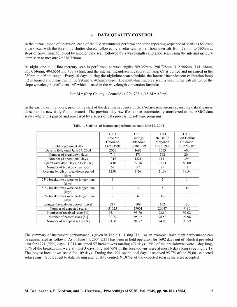
Table 1. Statistics of instrument performance until June 14, 2004

U111 Table Mt. Colorado

U211 Billings

Oklahoma

U311 Beltsville Maryland

U411 Fort Collins

Colorado Field deployment date 11/23/1998 10/28/1999 11/25/1999 10/22/2002

Days in field until June 14, 2004 2056 1692 1653 600 Number of breakdown days 740 471 542 204 Number of operational days 1316 1221 1111 396

Operational days/Days in field [%] 64.01 72.16 67.21 66.00 Number of breakdown periods 57 57 25 11

Average length of breakdown period [days]

12.98 8.26 21.68 18.54

25% breakdowns were no longer than [days]

1 1 2 1


2 3 5 6


7 6 16 17

Longest breakdown period [days] 217 109 162 130 Number of expected scans 31025 29001 26047 9180

Number of received scans [%] 93.14 95.70 98.60 97.02 Number of parsed scans [%] 92.72 95.27 98.53 96.96

Number of accepted scans [%] 91.31 91.87 94.06 93.59 The summary of instrument performance is given in Table 1. Using U211 as an example, instrument performance can be summarized as follows. As of June 14, 2004 U211 has been in field operation for 1692 days out of which it provided data for 1221 (72%) days. U211 sustained 57 breakdowns totaling 471 days. 25% of the breakdowns were 1 day long, 50% of the breakdowns were at most 3 days long and 75% of the breakdowns were at most 6 days long (See Figure 1). The longest breakdown lasted for 109 days. During the 1221 operational days it received 95.7% of the 29,001 expected solar scans. Subsequent to data parsing and quality control, 91.87% of the expected solar scans were accepted.


100

80

60

40

20

0

1/1/99 9/1/99 5/1/00 1/1/01 9/1/01 5/1/02 1/1/03 9/1/03 5/1/04Date [mm/dd/yy]

30

28

26

24

22

20

18

100

80

60

40

20

0

30

28

26

24

22

20

18

100

80

60

40

20

30

28

26

24

22

20

18

100

80

60

40

20

30

28

26

24

22

20

18

rhs axis: Number of expected scans lfs axis: Parsed scans to expected scans U-411: Fort Collins, CO

U-311: Beltsville, MA

U-211: Billings, OK

U-111: Table Mountain, CO

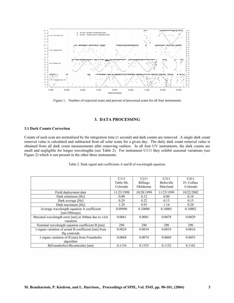
Figure 1. Number of expected scans and percent of processed scans for all four instruments

3. DATA PROCESSING 3.1 Dark Counts Correction Counts of each scan are normalized by the integration time (1 second) and dark counts are removed. A single dark count removal value is calculated and subtracted from all solar scans for a given day. The daily dark count removal value is obtained from all dark count measurements after removing outliers. In all four UV instruments, the dark counts are small and negligible for longer wavelengths (see Table 2). For instrument U111 they exhibit seasonal variations (see Figure 2) which is not present in the other three instruments.

Table 2. Dark signal and coefficients A and B of wavelength equation.

U111

Table Mt. Colorado

U211 Billings

Oklahoma

U311 Beltsville Maryland

U411 Ft. Collins Colorado

Field deployment date 11/23/1998 10/28/1999 11/25/1999 10/22/2002 Dark minimum [Hz] 0.00 0.12 0.00 0.10 Dark average [Hz] 0.29 0.22 0.13 0.15

Dark maximum [Hz] 1.29 0.93 1.14 0.28 Average wavelength equation A coefficient

[nm/200steps] 0.09996 0.10000 0.10001 0.10002

Maximal wavelength error [nm] at 360nm due to ±∆A variation

0.0061 0.0081 0.0078 0.0029

Nominal wavelength equation coefficient B [nm] 290 290 290 290 1-sigma variation of actual B coefficient [nm] from

Hg centroids 0.0024 0.0034 0.0019 0.0016

1-sigma variation of B [nm] from Fraunhofer algorithm

0.0068 0.0074 0.0069 0.0053

B(Fraunhofer)-B(centroids) [nm] 0.1154 0.1355 0.1152 0.1101


3.2 Wavelength Equation The solar spectrum is measured at p=0,…,700 grating positions nominally every 0.1nm (200 steps of stepper motor). A slight, though detectable (±0.001nm), nonlinearity in steps-to-wavelength equation can be neglected. The linear wavelength equation is used:

λp=Ap+B p=0,…,700

where A = M∆Step for ∆Step = 200. The wavelength equation coefficients A and B are obtained through two separate methods. The coefficient A is obtained from a linear fit between centroids and wavelengths of the mercury lines at 289.359nm, 296.728nm, 312.566nm, 334.148nm, 365.015nm, 404.656nm and 407.781nm. The centroids are obtained from the once-a-day multi-line mercury scan that is performed at night. The slope M is accepted if at least 3 “good” centroids are obtained. Then A is smoothed with an RC filter (see Figure 2). In Table 2 the average values of A vary from 0.09996 to 0.10002 between the four instruments (all 5 digits are significant). The instantaneous values of A are very stable. The error in A has the largest impact at 360nm (p=700). If A were not measured at all, but rather the average value were used instead for the duration of deployment, the wavelength errors at 360nm would be less than ±0.0061nm (see U111 in Table 2). The wavelength coefficient B is obtained from processing the centroids of the 296.278nm mercury line that is scanned once for each solar scan. The centroid is estimated using the first moment and dual slope methods, and the resolution (FWHM) of this line is calculated. The data is rejected if the centroids from the two methods differ by more than 0.0025nm or if the FWHM departs from the nominal value by more than 0.004nm. Then the remaining first moments are interpolated to generate the B coefficient for every solar scan in the daily file. In cases where all centroids are rejected, the centroid that violates the rejection criterion the least is used for the entire daily data.

1.2

0.8

0.4

0.0

3/1/99 9/1/99 3/1/00 9/1/00 3/1/01 9/1/01 3/1/02 9/1/02 3/1/03 9/1/03 3/1/04Date [mm/dd/yy]

99.98

99.97

99.96

99.95

99.94

x10

-3

290.4

290.2

290.0

289.8

289.6

Starting scan wavelength (B-coefficient) [nm] From Hg 296.728nm line [nm in air] From Fraunhofer algorithm [nm in vacuum]

Daily dark signal values [Hz]

A-Coefficient [nm/200steps] Daily from Hg scan Filtered and smoothed

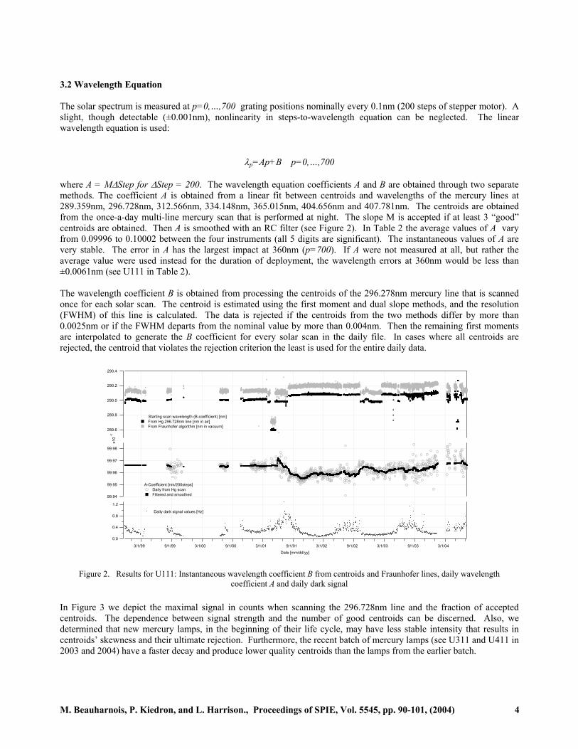
Figure 2. Results for U111: Instantaneous wavelength coefficient B from centroids and Fraunhofer lines, daily wavelength coefficient A and daily dark signal

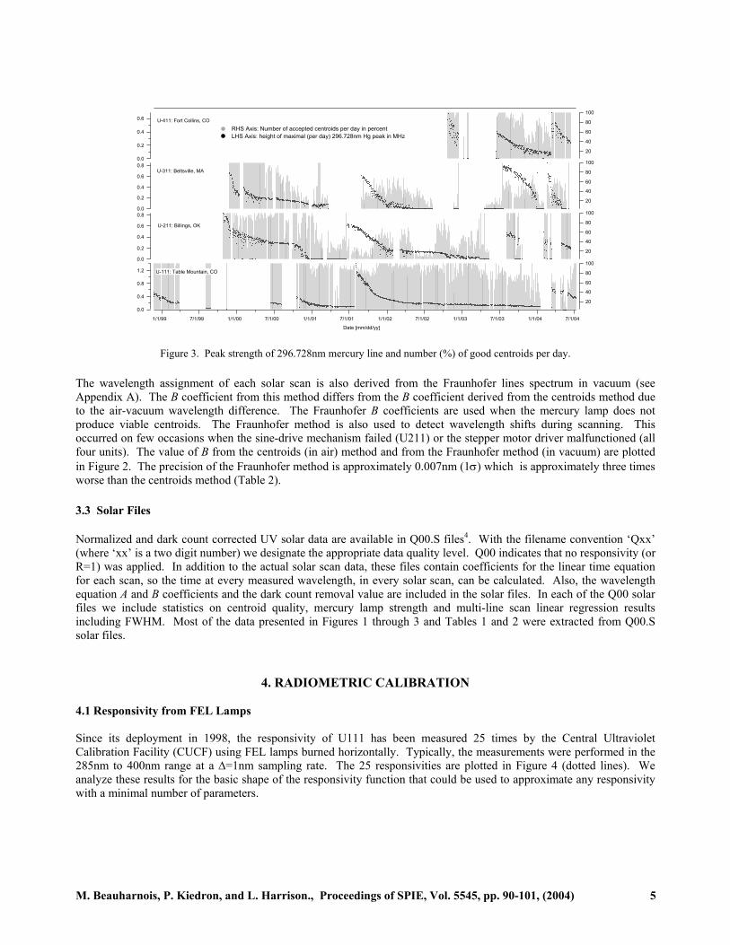
In Figure 3 we depict the maximal signal in counts when scanning the 296.728nm line and the fraction of accepted centroids. The dependence between signal strength and the number of good centroids can be discerned. Also, we determined that new mercury lamps, in the beginning of their life cycle, may have less stable intensity that results in centroids’ skewness and their ultimate rejection. Furthermore, the recent batch of mercury lamps (see U311 and U411 in 2003 and 2004) have a faster decay and produce lower quality centroids than the lamps from the earlier batch.


100

80

60

40

20

1/1/99 7/1/99 1/1/00 7/1/00 1/1/01 7/1/01 1/1/02 7/1/02 1/1/03 7/1/03 1/1/04 7/1/04

Date [mm/dd/yy]

0.8

0.6

0.4

0.2

0.0

100

80

60

40

20

0.8

0.6

0.4

0.2

0.0

100

80

60

40

20

0.6

0.4

0.2

0.0

100

80

60

40

20

1.2

0.8

0.4

0.0

U-411: Fort Collins, CO

U-311: Beltsville, MA

U-211: Billings, OK

U-111: Table Mountain, CO

RHS Axis: Number of accepted centroids per day in percent LHS Axis: height of maximal (per day) 296.728nm Hg peak in MHz

Figure 3. Peak strength of 296.728nm mercury line and number (%) of good centroids per day. The wavelength assignment of each solar scan is also derived from the Fraunhofer lines spectrum in vacuum (see Appendix A). The B coefficient from this method differs from the B coefficient derived from the centroids method due to the air-vacuum wavelength difference. The Fraunhofer B coefficients are used when the mercury lamp does not produce viable centroids. The Fraunhofer method is also used to detect wavelength shifts during scanning. This occurred on few occasions when the sine-drive mechanism failed (U211) or the stepper motor driver malfunctioned (all four units). The value of B from the centroids (in air) method and from the Fraunhofer method (in vacuum) are plotted in Figure 2. The precision of the Fraunhofer method is approximately 0.007nm (1σ) which is approximately three times worse than the centroids method (Table 2).

3.3 Solar Files Normalized and dark count corrected UV solar data are available in Q00.S files4. With the filename convention ‘Qxx’ (where ‘xx’ is a two digit number) we designate the appropriate data quality level. Q00 indicates that no responsivity (or R=1) was applied. In addition to the actual solar scan data, these files contain coefficients for the linear time equation for each scan, so the time at every measured wavelength, in every solar scan, can be calculated. Also, the wavelength equation A and B coefficients and the dark count removal value are included in the solar files. In each of the Q00 solar files we include statistics on centroid quality, mercury lamp strength and multi-line scan linear regression results including FWHM. Most of the data presented in Figures 1 through 3 and Tables 1 and 2 were extracted from Q00.S solar files.

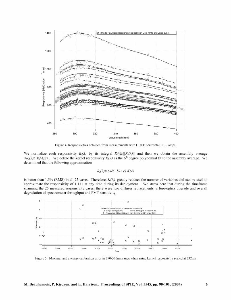
4. RADIOMETRIC CALIBRATION 4.1 Responsivity from FEL Lamps Since its deployment in 1998, the responsivity of U111 has been measured 25 times by the Central Ultraviolet Calibration Facility (CUCF) using FEL lamps burned horizontally. Typically, the measurements were performed in the 285nm to 400nm range at a ∆=1nm sampling rate. The 25 responsivities are plotted in Figure 4 (dotted lines). We analyze these results for the basic shape of the responsivity function that could be used to approximate any responsivity with a minimal number of parameters.


1400

1200

1000

800

600

400

Res

pons

ivity

[Hz/

(mW

/m2/n

m)]

400380360340320300280Wavelength [nm]

U-111: 25 FEL based responsivities between Dec. 1998 and June 2004

Figure 4. Responsivities obtained from measurements with CUCF horizontal FEL lamps.

We normalize each responsivity Ri(λ) by its integral Ri(λ)/||Ri(λ)|| and then we obtain the assembly average <Ri(λ)/||Ri(λ)||>. We define the kernel responsivity K(λ) as the 6th degree polynomial fit to the assembly average. We determined that the following approximation

Ri(λ)≈ (aλ2+bλ+c) K(λ)

is better than 1.5% (RMS) in all 25 cases. Therefore, K(λ) greatly reduces the number of variables and can be used to approximate the responsivity of U111 at any time during its deployment. We stress here that during the timeframe spanning the 25 measured responsivity cases, there were two diffuser replacements, a fore-optics upgrade and overall degradation of spectrometer throughput and PMT sensitivity.

5

4

3

2

1

0

Diff

eren

ce [%

}

1/1/99 7/1/99 1/1/00 7/1/00 1/1/01 7/1/01 1/1/02 7/1/02 1/1/03 7/1/03 1/1/04Date

Maximum difference [%] in 290nm-360nm interval Single point [332nm] min=0.24<avg=1.75<max=4.88 Two points [300nm,322nm] min=0.04<avg=0.51<max=1.69

Figure 5. Maximal and average calibration error in 290-370nm range when using kernel responsivity scaled at 332nm


In the narrower solar scan spectral range of 290nm to 360nm, we tested whether even simpler approximations using two parameters: (bλ+c)K(λ) and one parameter: cK(λ) are feasible. In Figure 5 the maximal error for two such approximations is depicted. In the two parameter case the estimate is forced to be equal to the estimated responsivity at wavelengths 300nm and 332nm. Within the assembly of 25 responsivity cases the maximal error is on average 0.5% and greater than 1% in only two cases. In the one parameter case the estimate and the estimated responsivity are forced to be equal at only 332nm. On average, the error is 1.75% and in three cases it is more than 3%. This demonstrates that if the responsivity is known at one or two wavelengths, as is the case when doing a vicarious calibration from a collocated UVMFRSR, the calibration of U111, with acceptable accuracy, is feasible.

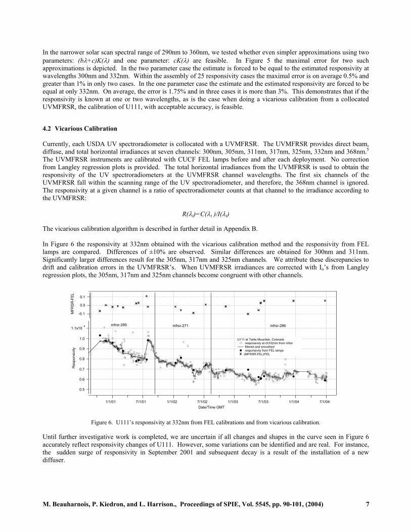
4.2 Vicarious Calibration Currently, each USDA UV spectroradiometer is collocated with a UVMFRSR. The UVMFRSR provides direct beam, diffuse, and total horizontal irradiances at seven channels: 300nm, 305nm, 311nm, 317nm, 325nm, 332nm and 368nm.5 The UVMFRSR instruments are calibrated with CUCF FEL lamps before and after each deployment. No correction from Langley regression plots is provided. The total horizontal irradiances from the UVMFRSR is used to obtain the responsivity of the UV spectroradiometers at the UVMFRSR channel wavelengths. The first six channels of the UVMFRSR fall within the scanning range of the UV spectroradiometer, and therefore, the 368nm channel is ignored. The responsivity at a given channel is a ratio of spectroradiometer counts at that channel to the irradiance according to the UVMFRSR:

R(λi)=C(λi )/I(λi) The vicarious calibration algorithm is described in further detail in Appendix B. In Figure 6 the responsivity at 332nm obtained with the vicarious calibration method and the responsivity from FEL lamps are compared. Differences of ±10% are observed. Similar differences are obtained for 300nm and 311nm. Significantly larger differences result for the 305nm, 317nm and 325nm channels. We attribute these discrepancies to drift and calibration errors in the UVMFRSR’s. When UVMFRSR irradiances are corrected with Io’s from Langley regression plots, the 305nm, 317nm and 325nm channels become congruent with other channels.

1.1x10 6

1.0

0.9

0.8

0.7

0.6

0.5

Res

pons

ivity

1/1/01 7/1/01 1/1/02 7/1/02 1/1/03 7/1/03 1/1/04 7/1/04Date/Time GMT

-0.1

0.0

0.1

MFR

SR-F

EL

mfrsr-286mfrsr-271mfrsr-289

U111 at Table Mountain, Colorado responsivity at ch332nm from mfrsr filtered and smoothed responsivity from FEL lamps(MFRSR-FEL)/FEL

Figure 6. U111’s responsivity at 332nm from FEL calibrations and from vicarious calibration. Until further investigative work is completed, we are uncertain if all changes and shapes in the curve seen in Figure 6 accurately reflect responsivity changes of U111. However, some variations can be identified and are real. For instance, the sudden surge of responsivity in September 2001 and subsequent decay is a result of the installation of a new diffuser.


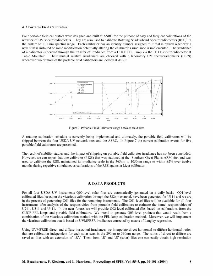
4. 3 Portable Field Calibrators

Four portable field calibrators were designed and built at ASRC for the purpose of easy and frequent calibrations of the network of UV spectroradiometers. They are also used to calibrate Rotating Shadowband Spectroradiometers (RSS)7 in the 360nm to 1100nm spectral range. Each calibrator has an identity number assigned to it that is retired whenever a new bulb is installed or some modification potentially altering the calibrator’s irradiance is implemented. The irradiance of a calibrator is derived through the transfer of irradiance from a CUCF FEL lamp via the U111 spectroradiometer at Table Mountain. Their mutual relative irradiances are checked with a laboratory UV spectroradiometer (U369) whenever two or more of the portable field calibrators are located at ASRC.

U-111

U-211

U-311

U-411

10/1/01 1/1/02 4/1/02 7/1/02 10/1/02 1/1/03 4/1/03 7/1/03 10/1/03 1/1/04 4/1/04Date

Calibration eventswith Portable Calibrators

P128 P130 P131 P132 P133

Figure 7. Portable Field Calibrator usage between field sites

A rotating calibration schedule is currently being implemented and ultimately, the portable field calibrators will be shipped between the four USDA UV network sites and the ASRC. In Figure 7 the current calibration events for five portable field calibrators are presented.

The result of stability studies and the impact of shipping on portable field calibrator irradiance has not been concluded. However, we can report that one calibrator (P128) that was stationed at the Southern Great Plains ARM site, and was used to calibrate the RSS, maintained its irradiance scale in the 365nm to 1050nm range to within ±2% over twelve months during repetitive simultaneous calibrations of the RSS against a Licor calibrator.

5. DATA PRODUCTS

For all four USDA UV instruments Q00-level solar files are automatically generated on a daily basis. Q01-level calibrated files, based on the vicarious calibration through the 332nm channel, have been generated for U111 and we are in the process of generating Q01 files for the remaining instruments. The Q01-level files will be available for all four instruments after analysis of the responsivities from portable field calibrators to estimate the kernel responsivities of U211, U311 and U411. In the near future, we will provide Q02-level calibrated files based on calibrations from the CUCF FEL lamps and portable field calibrators. We intend to generate Q03-level products that would result from a combination of the vicarious calibration method with the FEL lamp calibration method. Moreover, we will implement the vicarious calibration that is based on UVMFRSR irradiances corrected by means of Langley regression.

Using UVMFRSR direct and diffuse horizontal irradiances we interpolate direct horizontal to diffuse horizontal ratios that are calibration independent for each solar scan in the 290nm to 360nm range. The ratios of direct to diffuse are saved as files with an extension of ‘.R’.4 Then, from ‘.R’ and ‘.S’ (solar) files one can easily obtain high resolution


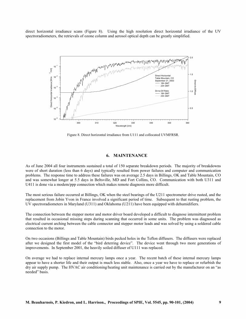
direct horizontal irradiance scans (Figure 8). Using the high resolution direct horizontal irradiance of the UV spectroradiometers, the retrievals of ozone column and aerosol optical depth can be greatly simplified.

10 -6

10 -5

10 -4

10 -3

10 -2

10 -1

Dire

ct H

oriz

onta

l Irra

dian

ce [W

/m2/n

m]

360350340330320310300Wavelength [nm]

2.0

1.5

1.0

0.5

Direct-to-D

iffuse

Direct HorizontalTable Mountain, COSeptember 21, 2003

18h GMT 23h GMT

Dir-to-Dif Ratio

18h GMT 23h GMT

Figure 8. Direct horizontal irradiance from U111 and collocated UVMFRSR.

6. MAINTENANCE

As of June 2004 all four instruments sustained a total of 150 separate breakdown periods. The majority of breakdowns were of short duration (less than 6 days) and typically resulted from power failures and computer and communication problems. The response time to address these failures was on average 2.5 days in Billings, OK and Table Mountain, CO and was somewhat longer at 5.5 days in Beltsville, MD and Fort Collins, CO. Communication with both U311 and U411 is done via a modem/ppp connection which makes remote diagnosis more difficult.

The most serious failure occurred at Billings, OK when the steel bearings of the U211 spectrometer drive rusted, and the replacement from Jobin Yvon in France involved a significant period of time. Subsequent to that rusting problem, the UV spectroradiometers in Maryland (U311) and Oklahoma (U211) have been equipped with dehumidifiers.

The connection between the stepper motor and motor driver board developed a difficult to diagnose intermittent problem that resulted in occasional missing steps during scanning that occurred in some units. The problem was diagnosed as electrical current arching between the cable connector and stepper motor leads and was solved by using a soldered cable connection to the motor.

On two occasions (Billings and Table Mountain) birds pecked holes in the Teflon diffusers. The diffusers were replaced after we designed the first model of the “bird deterring device”. The device went through two more generations of improvements. In September 2001, the heavily soiled diffuser of U111 was replaced.

On average we had to replace internal mercury lamps once a year. The recent batch of these internal mercury lamps appear to have a shorter life and their output is much less stable. Also, once a year we have to replace or refurbish the dry air supply pump. The HVAC air conditioning/heating unit maintenance is carried out by the manufacturer on an “as needed” basis.


Firmware upgrades have been made to all four UV instruments to facilitate the automatic operation of the portable field calibrators. With the exception of the field engineer having to place the portable calibrator over the diffuser and plug in the calibrator, these calibrations are intervention free. The general scanning schedule was not changed as a result of the firmware upgrades.

We also developed a web based system called “UV-CMATS” (“UV-Calibration, Maintenance and Tracking System”) to facilitate the logging of calibration, maintenance and upgrade events and also to track the location of the portable field calibrators.8

APPENDIX A: Wavelength Assignment from Fraunhofer lines

The SUSIM Atlas-3 extraterrestrial spectrum was used to provide the wavelength (in vacuum) registration for one selected clear sky spectrum of U111. This spectrum is denoted by M(p) where p=0,…700, and is referred to as a master spectrum. The resolution of the U111 spectrum was downgraded to match the resolution of the SUSIM spectrum and the low frequency components were removed from both SUSIM and M(p) to reduce the effects of varying sky irradiance when M(p) was measured. Then we determine a smooth and monotonically increasing mapping nmM(p)_—›_p that minimizes error residuals |SUSIM[nmM(p)]-M(p)|. Subsequently, all solar scans of U111 are compared against the master spectrum M(p) in its SUSIM based wavelength grid nmM(p).

To obtain the wavelength registration of any solar scan C(p), p=0,…700, the correlation method is used. First, both C(p) and M(p) have lower frequency components removed and are scaled to equalize amplitudes of Fraunhofer lines across the spectrum. The following assignment is used:

f_‹—_(f - smth(f))/smth(f)

Then the peak of the correlation function C M is located at ∆. The ∆ is the global wavelength shift between C and M in units of p. To detect finer nonlinear shifts (like rubber band effect) the same procedure is performed on shorter segments. First, to eliminate the effect of the global shift on the accuracy the following assignment is made:

C(p)=C(p-∆)

Then the correlation is performed on segments [64*i, 128+64*I] for i=0,..,10. Each correlation results in a shift ∆i. Results for some segments contain spurious noise and are gross outliers. They are rejected by using a linear fit ∆i=b+a*p, where p=64+64*i. Finally, a new wavelength assignment for scan C is obtained by interpolating nmM into a new grid b+a*p:

nmM(b+a*p)_—›_p=nmC(p)

APPENDIX B: Responsivity from Collocated UVMFRSR

Using the UVMFRSR filter function fn and uncalibrated counts C from the spectroradiometer the weighted averages Sn are calculated as follows:

Sn (tk ) = fn (λ i )Ck (λ i )∆λi

∑ n th − filter k th − scan


The responsivity is obtained as a ratio of Sn to irradiance In from the UVMFRSR. To take into account a possible asynchronization between the two collocated instruments and the effects of smoothing of the UVMFRSR signal, the ratios are calculated for different time offsets δ :

Rkn (δ) = Sn (tk ) / I n (tk −δ) δ = 0,±0.5' ,±1' ...± 5'

In principle, this method of calibration could be used with any fragment of the daily data. However, to minimize the effect of different angular responses (and/or cosine corrections) of the two collocated sensors the ratios in the vicinity of the solar noon are used (seven ratios within ±1.5 hours of solar noon):

Rn (δ) = Rkn (δ) / 7

Noon−tk <1.5h∑

ε(δ) = Rk

n (δ) − Rn (δ)( )2

Noon−tk <1.5h∑

The offset δ that minimizes the standard deviation ε(δ) is selected:

δ <5'minε(δ) ⇒ δ opt ⇒ Rn = Rn (δopt )

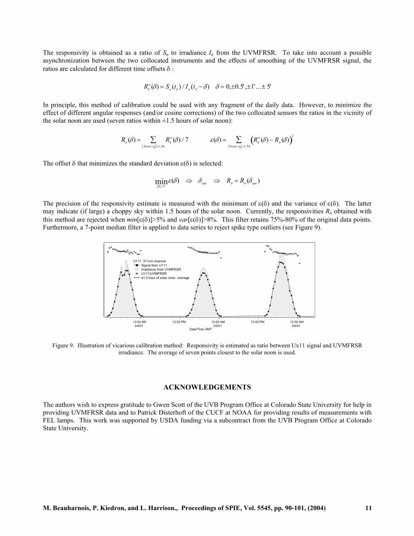
The precision of the responsivity estimate is measured with the minimum of ε(δ) and the variance of ε(δ). The latter may indicate (if large) a choppy sky within 1.5 hours of the solar noon. Currently, the responsivities Rn obtained with this method are rejected when min[ε(δ)]>5% and var[ε(δ)]>8%. This filter retains 75%-80% of the original data points. Furthermore, a 7-point median filter is applied to data series to reject spike type outliers (see Figure 9).

12:00 AM3/4/01

12:00 PM 12:00 AM3/5/01

12:00 PM 12:00 AM3/6/01

Date/Time GMT

x103

U111: 311nm channel Signal from U111 Irradiance from UVMFRSR U111/UVMFRSR ±1.5 hour of solar noon average

Figure 9. Illustration of vicarious calibration method: Responsivity is estimated as ratio between Ux11 signal and UVMFRSR irradiance. The average of seven points closest to the solar noon is used.

ACKNOWLEDGEMENTS

The authors wish to express gratitude to Gwen Scott of the UVB Program Office at Colorado State University for help in providing UVMFRSR data and to Patrick Disterhoft of the CUCF at NOAA for providing results of measurements with FEL lamps. This work was supported by USDA funding via a subcontract from the UVB Program Office at Colorado State University.



REFERENCES

1. K. Lantz, P. Disterhoft, E. Early, A. Thompson, J. DeLuisi, P. Kiedron, L. Harrison, J. Berndt, W. Mou, T.J. Ehramjian, L. Cabausua, J. Robertson, D. Hayes, J. Slusser, D. Bigelow, G. Janson, A. Beaubian, and M. Beaubian, “The 1997 North American interagency intercomparison of ultraviolet monitoring spectroradiometers”, J. Res. Natl. Inst. Stand. Technol., 107, 19-62, (2002).

2. L. Harrison, J. Berndt, P. Kiedron and P. Disterhoft, “United States Department of Agriculture reference ultraviolet spectroradiometer: current performance and operational experience at Table Mountain”, Colorado, Opt. Eng. 41(12), 3096-3103, (2002).

3. K. Lantz, P. Disterhoft, J. Slusser, J. Berndt, G. Bernhard, R. Booth, J. Ehramjian, W. Gao, L. Harrison, G. Janson, P. Johnston, P. Kiedron, R. McKenzie, M. Kimlin , J. Michalsky, P. Neale, M. O’Neill, V. Quang, G. Seckmeyer, T. Taylor, S. Wuttke, “The 2003 North American Interagency Intercomparison of Ultraviolet Spectroradiometers. PART A: Scanning and spectrograph instruments” (in preparation)

4. Solar files are available at: ftp://oink.asrc.cestm.albany.edu/pub/UX11/calibrated/ where X=1,2,3,4.

5. W. Gao, J. Slusser, J. Gobson, G. Scott, D. Bigelow, J. Kerr, B. McArthur, “Direct-Sun column ozone retrieval by the ultraviolet multifilter rotating shadow-band radiometer and comparison with those from Brewer and Dobson spectrophotometers, Appl. Opt. 40, 3149-3155, (2001).

6. Calibration files are available at ftp://oink.asrc.cestm.albany.edu/pub/UX11/lampscans/ where X=1,2,3,4.

7. L. Harrison , M. Beauharnois, J. Berndt, P. Kiedron, J. Michalsky, and Q. Min, The rotating shadowband spectroradiometer (RSS) at SGP, Geophys. Res. Lett., 26, 1,715-1,718, 1999.

8. UV-Calibration, Maintenance and Tracking System: http://hpc1.asrc.cestm.albany.edu/~cmats/cmats.php

ftp://oink.asrc.cestm.albany.edu/pub/UX11/calibrated/

ftp://oink.asrc.cestm.albany.edu/pub/UX11/lampscans/

the usda high-resolution uv radiation network:...

Documents