The University of Bradford Institutional Repository

http://bradscholars.brad.ac.uk

This work is made available online in accordance with publisher policies. Please refer to the

repository record for this item and our Policy Document available from the repository home

page for further information.

To see the final version of this work please visit the publisher’s website. Access to the

published online version may require a subscription.

Link to publisher’s version: http://dx.doi.org/10.1016/j.neucom.2016.07.050

Citation: Tehlah N, Kaewpradit P and Mujtaba IM (2016) Artificial neural network based

modelling and optimization of refined palm oil process. Neurocomputing. 216: 489-501.

Copyright statement: © 2016 Elsevier B.V. Reproduced in accordance with the publisher's self-

archiving policy. This manuscript version is made available under the CC-BY-NC-ND 4.0 license.

1

Artificial Neural Network based Modelling and Optimization of Refined Palm Oil

Process

N. Tehlaha, P. Kaewpradit

a, I.M. Mujtaba

b,*

aDepartment of Chemical Engineering, Prince of Songkla University, Songkhla 90112 THAILAND

bSchool of Engineering, University of Bradford, West Yorkshire BD7 1DP, UK

*Corresponding author.E-mail address: I.M.Mujtaba@bradford.ac.uk (I.M. Mujtaba)

Abstract

The content and concentration of beta-carotene, tocopherol and free fatty acid is one

of the important parameters that affect the quality of edible oil. In simulation based studies

for refined palm oil process, three variables are usually used as input parameters which are

feed flow rate (F), column temperature (T) and pressure (P). These parameters influence the

output concentration of beta-carotene, tocopherol and free fatty acid. In this work, we

develop 2 different ANN models; the first ANN model based on 3 inputs (F, T, P) and the

second model based on 2 inputs (T and P). Artificial neural network (ANN) models are set up

to describe the simulation. Feed forward back propagation neural networks are designed

using different architecture in MATLAB toolbox. The effects of numbers for neurons and

layers are examined. The correlation coefficient for this study is greater than 0.99; it is in

good agreement during training and testing the models. Moreover, it is found that ANN can

model the process accurately, and is able to predict the model outputs very close to those

predicted by ASPEN HYSYS simulator for refined palm oil process. Optimization of the

refined palm oil process is performed using ANN based model to maximize the concentration

of beta-carotene and tocopherol at residue and free fatty acid at distillate.

Keywords: Artificial Neural network; Refined palm oil process, Falling film molecular

distillation; Modelling; Optimization

1. Introduction

Molecular distillation (MD) is a special separation technique [1], and it is widely

used in various process such as in pharmaceutical, waste water treatment, food and biological

processes [2]. MD operates under vacuum pressure and lower temperature than conventional

process, which can prevent decomposition of materials and enhance the quality of product [3,

4]. Moreover, the MD is normally applied for thermally sensitive materials. Three

parameters are important which add value to the palm oil and these are tocopherol and beta-

2

carotene in the bottom stream and contaminant of free fatty acid in the distillate stream. In

conventional deodorization of palm oil process, the high temperature operation not only

eliminates the free fatty acid from oil but also destroy some of the phytonutrients such as

beta-carotene and tecopherol due to their thermal sensitive nature. However, the

deodorization of palm oil by MD can overcome the problem. The purpose of this work is to

obtain the optimum process parameters in order to recovery high concentration of beta-

carotene and tocopherol at residue and free fatty acid at the distillate stream. In previous

studies [5-8] the operating variables that affect to quality of oil in molecular distillation are

feed flow rate, column temperature, pressure, rolling speed and etc. However, only feed flow

rate, pressure and temperature affect the quality of oil in falling film molecular distillation.

Moreover, other inputs such as condenser temperature and ambient temperature

insignificantly affect to the quality of the oil.

In the absence of a real palm oil MD process, the input-output data for the process

(required for developing NN based model) is generated via ASPEN HYSYS simulator. The

development of MD in ASPEN HYSYS follows similar procedure of literature work where

an MD model for palm oil process was developed using ASPEN PLUS (one flash vessel) and

validated the results with DISMOL [9]. In their study binary equimolar mixture of Dibutyl

phthalate (DBP) and Dibutyl sebacate (DBS) were fed at 50 kg/hr and 0.133 Pa. Temperature

was manipulated to accomplish identical distillation mass ratio (0.2120) with DISMOL. The

operating temperature for DISMOL and ASPEN PLUS to achieve the same distillate mass

ratio were reported to be 369 K and 336 K [9] respectively and with ASPEN HYSYS[10] it

was found to be 335.66 K which is close to that obtained by ASPEN PLUS. The results from

DISMOL, ASPEN PLUS and ASPEN HYSYS are shown in (Fig.1).

Fig. 1: The simulation results for DISMOL, ASPEN PLUS and Developed ASPEN HYSYS

0

0.2

0.4

0.6

0.8

1

0 1 2 3

Mss

ra

tio

, m

ola

r fr

act

ion

DISMOL

ASPEN PLUS

ASPEN HYSYS

Distillate mass ratio Residue DBP

molar fration Distillate DBP

molar fraction

3

It is clear that the results of ASPEN HYSYS simulation are comparable to those

DISMOL and ASPEN PLUS in term of distillation mass ratio, distillate DBP molar fraction

and residue DBP molar fraction. Hence, the ASPEN HYSYS simulator can be applied to any

process related with MD such as MD for palm oil considered in this work.

The deodorization of refined palm oil process is simulated via ASPEN HYSYS model

developed following the procedure outlined in [9] and validated with patent of Refining of

edible oil rich in natural carotenes [11]. The results were found to be in good agreement for

each simulation results which efficiency errors are less than 3% [10].

In the past, ANN based models have been considered as possible alternatives to

predict process behaviors with molecular distillation and crude oil distillation [7, 12-14]. In

this work ANN models based on 3 inputs and 2 inputs are constructed to facilitate operational

optimization of MD in deodorization of refined palm oil process. The architectures of neural

networks (NN) are investigated by studying the effect of layers, hidden layers and number of

neurons in each layer. Transfer function for NN performance is also examined to give the

best predictions for NN architecture. The resulting model is then incorporated in optimization

to determine the operating conditions in MD column that maximize the quality of palm oil.

Note, ASPEN HYSYS model is used to generate input-out data of the process to be used in

ANN model.

Finally, the contribution and the novelty of this work have been highlighted as:

Falling film molecular distillation (MD) model for refined palm oil process has been

developed from the single flash vessel in ASPEN HYSYS simulator. Since, there is

no module available in the ASPEN HYSYS simulator, developed MD simulation has

been validated with patent’s data of refining of edible oil rich in natural carotene. The

simulation results are in good agreement with those of the patent.

The required data for developing ANN model is generated via simulation of the

developed MD model using ASPEN HYSYS simulator. Even though, there are many

literatures ton the simulation of MD, the MD model for deodorization of palm oil

process has not been carried out before.

4

2. MD Process for the Palm Oil

Fig. 2: Schematic Diagram of a Molecular distillation process

A process for production of palm oil consists of 3 main parts, which are degumming,

bleaching and deodorization. Degumming is a process of removing phospatide from crude

oil, and then the degummed oil is treated by bleaching earth before entering the deodorization

column. Schematic diagram of MD is shown in (fig. 2). The MD column mainly consists of

evaporator and internal condenser. In the MD column, high vacuum is achieved by vacuum

booster pump. The liquid from feed stream is degassed by degasser unit and then enter the

heated evaporator [15]. The heated liquid enters the MD as vapor phase. Each molecule has

different moving distance; light molecule has longer mean free path than the heavy molecule.

The longer mean free path provides more capability for molecule to reach the condenser

board. The lighter molecule will condense and leave the column through the distillate stream.

However, the heavy molecule will leave via the residue stream. In this work, beta-carotene

and tocopherol are heavy substances; they will leave the MD column through the residue

stream, whereas free fatty acid is lighter and leaves the MD column through the distillate

stream. Usually feed flow rate (F), column temperature (T) and pressure (P) influence the

output concentration of beta-carotene, tocopherol and free fatty acid. The product quality

Residue

Feed stream

Cooling water Cooling water

Con

den

ser

Vacuum

Distillate

Hea

ting

boar

d

Hea

ting

boar

d

5

(beta-carotene and tocopherol concentration at residue) increases with decreasing

temperature, on the other hand with increasing pressure, according to (equation 1.)

𝜆 =𝑅𝑇

√2𝜋𝑑2𝑁𝐴𝑃 (1)

Where 𝜆 is the mean free path, R is gas constant, T is temperature, P is the pressure, NA is

Avogadro’s number and d is molecular diameter.

Mean free path is function of both temperature and pressure. Increasing temperature increases

the mean free path; thus the heavy molecules (beta-carotene and tocopherol) can more easily

reach the condenser. Consequently, they leave the column through the distillate stream;

hence, the quality of edible oil is decreased. But the effect of pressure is opposite; the heavy

molecules cannot more easily reach the condenser, therefore product quality is increased.

With the increasing feed flow rate, the product quality decline. Increasing feed flow rate

results in shorter residence time. The lighter molecule (FFA) could not evaporate timely, and

therefore, it remains in the residue. Consequently, the quality of edible oil decreases because

the FFA contaminates the residue stream.

3. ANN modeling

Artificial neural network (ANN) is widely accepted as alternative technique to capture

and represent the complicated input and output relationship of processes [16]. It is an

information processing system that does not have to be programmed and non-algorithmic.

ANN models are applied in various applications such as process control, system

identification, business, modeling, pattern recognition and simulation. It performs intellectual

tasks similar to human brain by acquires knowledge during learning and stores within inner

neuron. The significance of using neural network is in its easy to perform feature for

developing a process model. Since the process is nonlinear, so it is difficult to solve

manually. Conversely, the first principle modeling requires knowledge to calculate physical

properties for developing model. In addition, neural network model is less computationally

expensive than 1st principle model. The neural network consists of neurons in different layers

within the network, which are input layer, one or more hidden layers and output layer. The

neuron network essentially receives input data (signal), train and processes then sends outputs

signal. Each input is weighted, and its weight (w) is relying on the particular input. The

weights and biases (b) are the connection among input, neurons and outputs of the neural

6

network. The weights and biases are then summed and added up by a transfer function into

one or more outputs depending on the process.

3.1 Neural network architecture and training

In this study, feed forward network is used to solve the approximation fitting problem.

Multi-layer perception (MLP) network is the most common and famous type of feed forward

network. Feed forward network is a straight forward network that travel only one way (no

feedback loop), and it is a supervisory network that requires outputs in order to learn. The

architecture of neural network for multi-input and multi- output is shown in Fig. 3, where i is

number of elements in input, and j is number of neurons in layer. The summation of weight

inputs (wx) with biases (b) are the argument of transfer function (f); hyperbolic tangent

sigmoid transfer function (tansig) and linear transfer function (purelin), which produces the

output (y). In addition, the outputs of each transitional layer are the input of the subsequent

layer.

Back propagation algorithm based on Levenberg-Marquardt (trainlm) is the training

function used in order to train the network [17]. This algorithm is the most commonly used

procedure to determine the error derivative of the weight. Before starting the network design,

it is important to ensure that the training data cover the range of input space. It is because the

neural network is skillful in interpolation rather that extrapolation of data [18, 19].

Fig. 3: Neural network architecture for 1st ANN model

The output variables of the 1st ANN model can be calculated and written as:

𝑦𝑘 𝑠𝑐𝑎𝑙𝑒𝑢𝑝 = 𝑓2(𝑎𝑘2) (2)

7

𝑎𝑘2 = (∑ 𝑤2

𝑗𝑘 × 𝑓1(𝑎𝑗1)) + 𝑏2

𝑘20𝑗=1 (3)

𝑎𝑗1 = (∑ 𝑤1

𝑖𝑗 × 𝑥𝑖) + 𝑏1𝑗

3𝑖=1 (4)

Where

i is the number of input variables.

j is the number of neurons.

k is the number of output variables.

𝑎1 and 𝑎2 are linear combiner outputs of 1st hidden layer and outputs layer

respectively.

𝑏1and 𝑏2 are the bias of 1st hidden layer and output layer respectively.

𝑤1and 𝑤2 are the synaptic weight of neuron for 1st hidden layer and output

layer respectively.

𝑓1 is transfer function for hidden layer.

𝑓2 is transfer function for output layer.

Lastly, the output values are calculated or de-normalized to the original units

by equation

𝑦𝑘 = (𝑦𝑘 𝑠𝑐𝑎𝑙𝑒𝑢𝑝 x 𝑦𝑘 𝑠𝑡𝑑) + 𝑦𝑘 𝑚𝑒𝑎𝑛 (5)

Where 𝑦𝑘 = output variables

𝑦𝑘 𝑠𝑐𝑎𝑙𝑒𝑢𝑝 = scaleup output variables

𝑦𝑘 𝑠𝑡𝑑 = standard deviation of scaleup output variables

𝑦𝑘 𝑚𝑒𝑎𝑛 = average of scaleup output variables

An effective ANN model can be developed if the design variables and its responses

are normalized. The input variables and output variable are normalized before training in

order to avoid the over fitting. The input data are normalized and scaled up as follows

x1 scaleup Feed flow rate scaleup

x2scaleup = Temperature scaleup

x3scaleup Pressure scaleup

Where i is number of input variables

The normalized output variables in the neural network correlation are as follows:

8

y1 scaleup Beta-carotene scaleup

y2 scaleup = Tocopherol scaleup

y3 scaleup Free fatty acid scaleup

𝑥𝑖 𝑠𝑐𝑎𝑙𝑒𝑢𝑝 =𝑥𝑖−𝑥𝑖 𝑚𝑒𝑎𝑛

𝑥𝑖 𝑠𝑡𝑑 (6)

Where ximean, is the average of input variables.

xistd is the standard deviation of input variables,

The standard deviation of each input variable is calculated as follows:

𝑥𝑖𝑠𝑡𝑑 = √(∑(𝑥𝑖−𝑥𝑖𝑚𝑒𝑎𝑛

)2

𝑛−1) (7)

Where n is total number of data

i is input variables

The normalization of data accelerates the training process, and also improves capabilities of

the network [20].

Sensitivity analysis or input variable analysis is used and applied in this part as a

technique to eliminate the least impact on the process. It is a technique that assists by

focusing only on significant effect of input variables to the process. In this part, a partial

modeling is applied to estimate the sensitivity of predicted responses. Varying pressure and

temperature have largest effects on the outputs; nevertheless, feed flow rate has less effect on

any of outputs. It can be concluded that x2 and x3 are significant variables, whereas x1 is

insignificant variable.

Later, in this work, we develop 2 difference models; the first ANN model (1st ANN)

based on 3 inputs (x1, x2, x3) and 3 outputs: concentration of beta-carotene and tocopherol at

residue and free fatty acid at distillated stream (y1 , y2, y3) and the second ANN model (2nd

ANN) based on 2 inputs (x2, x3) without considering insignificant variable and 3 outputs (y1 ,

y2, y3). The ANN model is developed and the effects of numbers of neuron and hidden layer

are discussed. In this study different inputs are generated from the ASPEN HYSYS

simulation of refined palm oil process to be used to develop the artificial neural network

(ANN) models. The 70% of input data are used for training (bold), 15% data are used for

9

testing (normal) and the remaining 15% data (italic) are used for validation (Table C,

Appendix). The training, testing, and validation is executed to estimate the performance of

neural network [21] for forecasting the concentration of beta-carotene (y1), tocopherol (y2),

and free fatty acid(y3), in order to estimate the quality of edible oil, in terms of value added

and contaminant. The input variables and its statistics for the first ANN model and second

ANN model are shown in Table 1 and 2 respectively. The feed flow rate for first model is in

the range of 1000-2000 kg/hr, for both models, temperature and pressure are in the range of

100-200oC and 0.00000-0.001 kPa respectively.

Table1

Statistical data for input variables and its output for 1st ANN model.

MEAN STD Variables range

Scaleup

range

Feed flow rate (kg/hr) 1500 409.49 1000-2000 -1.221-1.221

Column Temperature (oC) 150 35.46 100-200 -1.410-1.410

Column Pressure (kPa) 0.0005 0.000317 0-0.001 -1.576-1.576

Beta-carotene in residue (mass fraction) 3.88x10-4

0.000208 1.166x10-6

-5.6x10-4

-1.850-0.848

Tocopherol in residue (mass fraction) 6.27x10-4

0.000343 1.53x10-6

-9.10x10-4

-1.82-0.0826

Free fatty acid in distillate (mass fraction) 6.54x10-1

0.384413 0.061-1.00 -1.54-0.901

Table 2

Statistical data for input variables and its outputs for 2nd

ANN model.*

MEAN STD Variable

s range

Scaleup

range

Column Temperature (oC) 150 35.68 100-200 -1.410-1.410

Column Pressure (kPa) 0.0005 0.000319 0-0.001 -1.576-1.576

Beta-carotene in residue (mass fraction) 3.88 x10-4

0.000209 1.166x10-6

-5.6x10-4

-1.850-0.848

Tocopherol in residue (mass fraction) 6.27 x10-4

0.000345 1.53x10-6

-9.10x10-4

-1.82-0.0826

Free fatty acid in distillate (mass fraction) 6.54 x10-4

0.386778 0.061-1.00 -1.54-0.901

*without considering feed flow rate

4. Results and discussion

The number of neurons and layer are varied as shown in Table 3-4. The Mean square

error (MSE) is the measure of performance for the network, and the best ANN model is based

on the least mean square error. The network is trained, validated and tested by neural network

tool (nntool) in Matlab toolbox.

4.1 The effect of number of layers

The number of layer for 1st ANN and 2

nd ANN model is investigated with fixed 10

neurons. The effect of number of layers is shown in Tables 3-4. Increasing number of layers

from 3 to 10 with fixed number of neurons results in inaccuracy. The training is terminated at

10

sufficiently small value of the mean square error (MSE). They show that 2 and 3 layers

network has smaller MSE compared to others. The smallest MSE is for 2 layers network, it

gives very good values of the correlation data, and the training is stopped after 15 iteration

(epoch) and 12 iteration for 1st ANN and 2

nd ANN models respectively. However, increasing

the number of layers results in inaccurate predictions.

Table 3

Effect of number of layers on the network performance (1st ANN model)

2 layers 3 layers 10 layers

MSE 0.0125 0.4230 4.3700

Epoch 15 17 6

Table 4

Effect of number of layers on the network performance (2nd

ANN model)

2 layers 3 layers 10 layers

MSE 0.0287 0.0445 1.5138

Epoch 12 21 23

4.2 The effect of number of neurons

Having found out that the 2 layer network is the best, the effect of number of neurons

is investigated for this network (1 hidden layer and 1 output layer). The number of neurons is

varied from 1 to 25 neurons. The transfer functions used in this work are tansig (hyperbolic

tangent sigmoid transfer function) for the first layer and purelin (a linear transfer function)

for the second layer. The results for 1st and 2

nd ANN model are summarized in Figs 4-5. The

optimum number of neurons for 2 layers network are 20 neurons for both models.

Fig. 4: Validation MSE response for 1st ANN model with 2 layers

0.00

0.02

0.04

0.06

0.08

0.10

0.12

1 2 3 4 5 6 7 8 9 10 11 12 13 14 15 16 17 18 19 20 21 22 23 24 25

Mea

n s

qu

are

erro

r

Number of neurons

Mean square error

11

Fig. 5: Validation MSE response for 2nd

ANN model with 2 layers (without considering feed

flow rate)

Figs. 6-7 show the optimum regression plot of training, validation and testing for 1st

ANN model and 2nd

ANN model respectively. They show the relationship between the

network target and the output. It can be seen that, the regression is nearly equal to 1, which is

desirable. However, the performance evaluation of 20 neurons configuration is the best

although the 20 neurons network take longer iteration time to reach a target. The optimum

weight and bias for the 1st ANN model with 2 layers for 20 neurons are shown in Tables A,

and Tables B in appendix shows weight and bias for the 2nd

ANN model with 2 layers and 20

neurons.

Fig. 6:.The regression plot of training, validate, testing and the overall regression for 20

neurons (1st ANN model)

0.00

0.05

0.10

0.15

0.20

1 2 3 4 5 6 7 8 9 10 11 12 13 14 15 16 17 18 19 20 21 22 23 24 25

Mea

n squ

are e

rror

Number of neurons

Mean square error

12

Fig. 7: The regression plot of training, validate, testing and the overall regression for 20

neurons (2nd

ANN model)

4.2 ANN generalization

Neural networks with 2 layers (1 hidden layer and 1 output layer) and 20 neurons are

used to predict the outputs of beta-carotene and tocopherol at residue and free fatty acid at

distillate stream. The input data to predict the outputs are the data that have not been used

before for training, validation and testing. The 1st ANN model predicts the outputs

concentration at different F, T and P values that are outward the training, testing and

validation data, which are at 1100 kg/hr, 140oC and 0.00055 kPa respectively. The 2

nd ANN

model is also investigated at different T and P of 140oC and 0.00055 kPa respectively (T and

P values are same those used in the 1st ANN model). The results based on ANN are compared

with ASPEN HYSYS simulator as shown in Figs 8-22.

At constant F and T (Figs. 8-10), predicted outputs of 1st

ANN model are found to be

close to those predicted by ASPEN HYSYS simulator. The criteria used for evaluation is R-

square (R2) as follows:

𝑅2 = 1 −∑ (𝑦𝑝,𝑖−𝑦𝑜,𝑖)𝑛

𝑖=12

∑ (𝑦𝑜,𝑖−𝑦𝑜̅̅̅̅ )𝑛𝑖=1

2 (8)

Where yp,i is correlated value; yo,i is observed value; 𝑦𝑜̅̅̅ is average observed value and

R2 is a statistical measure used to measure the linear correlation between correlated and

measured value. The R2 of predicted outputs is 0.9. Also, prediction outputs of 2

nd ANN

model at constant T (Figs. 11-13) is found to be close to those predicted by ASPEN HYSYS

13

simulator but with R2

equal to 0.99 for all outputs. According to these (Figs. 8-13), elevated

pressure results in improved prediction of the outputs by both 1st and 2

nd ANN models. It is

important to note that the high pressure in MD column influences to shorter mean free path of

molecules (equation 1). The shorter mean free path offers less capability for molecules to

travel or reach the condensation board, therefore, less vaporization occurs. Consequently, it

increases the quality of edible oil.

At constant F and P (Figs. 14-16), the 1st ANN model displays accurate prediction

with R2 equal to 0.99 for all outputs. Also, at constant P, the 2

nd ANN model also predicts

precise outputs with R2 equal to 1 as shown in (Figs 17-19). These figures clearly show that

the predicted outputs decrease with increasing temperature. The increasing T unfortunately

reduces the concentration of beta-carotene and tocopherol and they are vaporized to distillate

stream. It is necessary to note that high temperature operation not only reduces the

concentration of beta-carotene and tocopherol but also destroys them due to temperature

sensitivity. Thus, high temperature reduces palm oil quality.

Figs. 20-22 depict the predicted outputs of 1st ANN model and ASPEN HYSYS

simulator at constant T and P. The concentrations of beta- carotene and tocopherol at residual

stream and free fatty acid at distillate show no significant difference. The R2 of 1

st ANN

model prediction and that with ASPEN HYSYS simulator are both equal to 1. However,

varying feed flow rates (different residence time) shows no significant differences (observed

by both ANN model and ASPEN HYSYS simulator).

The predictions by 2 different ANN models follow the expected prediction of ASPEN

HYSYS simulator. Lastly, these studies reveal that the proposed artificial neural networks

with 2 layer (1 hidden layer and 1 output layer) and 20 neurons in hidden layer are able to

predict the concentration of beta-carotene, tocopherol at residue and free fatty acid at

distillate accurately.

Moreover, it can be clearly seen that the prediction output of 1st ANN model is more

accurate than 2nd

ANN model. The next section focuses on the optimization of process design

based on optimum model.

14

Fig. 8: Predicted outputs of beta-carotene for 1st ANN model at constant feed flow rate (1100

kg/hr) and temperature (140 oC).

Fig. 9: Predicted outputs of tocopherol for 1st ANN model at constant feed flow rate (1100

kg/hr) and temperature (140 oC).

Fig. 10: Predicted outputs of free fatty acid for 1st ANN model at constant feed flow rate

(1100 kg/hr) and temperature (140 oC).

-1.500 -1.000 -0.500 0.000 0.500 1.000 1.500 2.000

0

0.1

0.2

0.3

0.4

0.5

0.6

0.7

0.8

0.9

1

0

0.1

0.2

0.3

0.4

0.5

0.6

0.7

0.8

0.9

1

-1.500 -1.000 -0.500 0.000 0.500 1.000 1.500 2.000

Sca

led

up

co

nce

ntr

ati

on

Bet

a-c

aro

ten

e

Scaledup pressure

ANN

ASPEN HYSYS

-1.500 -1.000 -0.500 0.000 0.500 1.000 1.500 2.000

00.10.20.30.40.50.60.70.80.91

00.10.20.30.40.50.60.70.80.9

1

-1.500 -1.000 -0.500 0.000 0.500 1.000 1.500 2.000

Sca

led

up

co

nce

ntr

ait

on

To

cop

her

ol

Scaleup pressure

ANN

ASPEN HYSYS

-1.500 -1.000 -0.500 0.000 0.500 1.000 1.500 2.000

0

0.1

0.2

0.3

0.4

0.5

0.6

0.7

0.8

0.9

1

0

0.1

0.2

0.3

0.4

0.5

0.6

0.7

0.8

0.9

1

-1.500 -1.000 -0.500 0.000 0.500 1.000 1.500 2.000

Sca

leu

p c

on

cen

tra

tio

n

Fre

e fa

tty

aci

d

Scaledup Pressure

ANN

ASPEN HYSYS

15

Fig. 11: Predicted outputs of beta-carotene for 2nd

ANN model at constant temperature

(140 oC).

Fig. 12: Predicted outputs of tocopherol for 2nd

ANN model at constant temperature (140 oC).

Fig. 13: Predicted outputs of free fatty acid for 2nd

ANN model at constant temperature

(140 oC).

-1.500 -1.000 -0.500 0.000 0.500 1.000 1.500 2.000

0

0.1

0.2

0.3

0.4

0.5

0.6

0.7

0.8

0.9

1

-0.2

0

0.2

0.4

0.6

0.8

1

-1.500 -1.000 -0.500 0.000 0.500 1.000 1.500 2.000

Sca

leu

p c

on

cen

tra

tio

n o

f

Bet

a-c

aro

ten

e

Scaleup pressure

ANN

ASPEN HYSYS

-1.500 -1.000 -0.500 0.000 0.500 1.000 1.500 2.000

0

0.1

0.2

0.3

0.4

0.5

0.6

0.7

0.8

0.9

1

0

0.1

0.2

0.3

0.4

0.5

0.6

0.7

0.8

0.9

1

-1.500 -1.000 -0.500 0.000 0.500 1.000 1.500 2.000

Sca

leu

p c

on

cen

tra

tio

n o

f

To

cop

her

ol

Scaleup pressure

ANN

ASPEN HYSYS

-1.500 -1.000 -0.500 0.000 0.500 1.000 1.500 2.000

0

0.2

0.4

0.6

0.8

1

1.2

0

0.2

0.4

0.6

0.8

1

1.2

-1.500 -1.000 -0.500 0.000 0.500 1.000 1.500 2.000

Sca

leu

p c

on

cen

tra

tio

n o

f

Fre

e fa

tty

aci

d

Scaleup pressure

ANN

ASPEN HYSYS

16

Fig. 14: Predicted outputs of beta-carotene for 1

st ANN model at constant feed flow rate

(1100 kg/hr) and pressure (0.00055 kPa)

Fig. 15: Predicted outputs of tocopherol for 1st ANN model at constant feed flow rate (1100

kg/hr) and pressure (0.00055 kPa)

Fig. 16: Predicted outputs of free fatty acid for 1st ANN model at constant feed flow rate

(1100 kg/hr) and pressure (0.00055 kPa)

-2 -1.5 -1 -0.5 0 0.5 1 1.5 2

-2

-1.5

-1

-0.5

0

0.5

1

-2

-1.5

-1

-0.5

0

0.5

1

-2 -1.5 -1 -0.5 0 0.5 1 1.5 2

Scaleup temperaute

Sca

leu

p

con

cen

tra

tio

n

Bet

a-

caro

ten

e

ANN

ASPEN HYSYS

-2 -1.5 -1 -0.5 0 0.5 1 1.5 2

-2

-1.5

-1

-0.5

0

0.5

1

-2

-1.5

-1

-0.5

0

0.5

1

-2 -1.5 -1 -0.5 0 0.5 1 1.5 2

Sca

leu

p

con

cen

tra

tio

n

To

cop

her

ol

Scaleup temperature

ANN

ASPEN HSYSY

-2 -1.5 -1 -0.5 0 0.5 1 1.5 2

-2

-1.5

-1

-0.5

0

0.5

1

1.5

-2

-1.5

-1

-0.5

0

0.5

1

1.5

-2 -1.5 -1 -0.5 0 0.5 1 1.5 2

Sca

leu

p c

on

cen

tra

tio

n

Fre

e fa

tty

aci

d

Scaleup temperature

ANN

ASPEN HYSYS

17

Fig. 17: Predicted outputs of beta-carotene for 2nd

ANN model

at constant pressure (0.00055 kPa)

Fig. 18: Predicted outputs of tocopherol for 2nd

ANN model

at constant pressure (0.00055 kPa)

Fig. 19: Predicted outputs of free fatty acid for 2nd

ANN model

at constant pressure (0.00055 kPa)

-2 -1.5 -1 -0.5 0 0.5 1 1.5 2

-2

-1.5

-1

-0.5

0

0.5

1

-2

-1.5

-1

-0.5

0

0.5

1

-2 -1.5 -1 -0.5 0 0.5 1 1.5 2S

cale

up

co

nce

ntr

ati

on

of

Bet

a-c

aro

ten

e

Scaleup Temperature

ANN

ASPEN HYSYS

-2 -1.5 -1 -0.5 0 0.5 1 1.5 2

-2

-1.5

-1

-0.5

0

0.5

1

-2

-1.5

-1

-0.5

0

0.5

1

-2 -1.5 -1 -0.5 0 0.5 1 1.5 2

Sca

leu

p c

on

cen

tra

tio

n o

f

Bet

a-c

aro

ten

e

Scaleup Temperature

ANN

ASPEN HYSYS

-2 -1.5 -1 -0.5 0 0.5 1 1.5 2

-2

-1.5

-1

-0.5

0

0.5

1

-2

-1.5

-1

-0.5

0

0.5

1

-2 -1.5 -1 -0.5 0 0.5 1 1.5 2

Sca

leu

p c

on

cen

tra

tio

n o

f

Bet

a-c

aro

ten

e

Scaleup Temperature

ANN

ASPEN HYSYS

18

Fig. 20: Predicted outputs of beta-carotene for 1st ANN model at constant

temperature (140 oC)and pressure (0.00055 kPa)

Fig. 21: Predicted outputs of free fatty acid for 1st ANN model at constant

temperature (140 oC)and pressure (0.00055 kPa)

Fig. 22: Predicted outputs of free fatty acid for 1st ANN model at constant

temperature (140 oC)and pressure (0.00055 kPa)

-1.5 -1 -0.5 0 0.5 1 1.5

0

0.2

0.4

0.6

0.8

1

1.2

1.4

0

0.2

0.4

0.6

0.8

1

1.2

1.4

-1.5 -1 -0.5 0 0.5 1 1.5Scaleup feed flow rate

Sca

leu

p c

on

cen

tra

tio

n

Bet

a-c

aro

ten

e

ANN

ASPEN HYSYS

-1.5 -1 -0.5 0 0.5 1 1.5

0

0.2

0.4

0.6

0.8

1

1.2

1.4

0

0.2

0.4

0.6

0.8

1

1.2

1.4

-1.5 -1 -0.5 0 0.5 1 1.5

Scaleup feed flow rate

Sca

leu

p c

on

cen

tra

tio

n

To

cop

her

ol

ANN

ASPEN HYSYS

-1.5 -1 -0.5 0 0.5 1 1.5

0

0.2

0.4

0.6

0.8

1

1.2

1.4

0

0.2

0.4

0.6

0.8

1

1.2

1.4

-1.5 -1 -0.5 0 0.5 1 1.5

Sca

leu

p c

on

cen

tra

tio

n

Fre

e fa

tty

aci

d

ANN

ASPEN HYSYS

19

4.3 Optimization of MD for refined palm oil process based on optimum ANN model

In this section, the aim is to find the optimum parameters of feed flow rate (x1),

column temperature (x2) and column pressure (x3) that maximize the quality of edible oil,

which depends on the recovery of beta-carotene (y1) and tocopherol (y2) in the residue and

contaminant removal of free fatty acid (y3) in the distillate. Maximization of the summation

of these (Equation 9) maximizes the quality of the oil. The mathematical model of the process

(Equation 9) is based on scaled-up ANN model. The upper bound and lower bound of

variables are specified based on values in Table 1.

Maximize: 𝑓(𝑦) = 𝑦1 𝑠𝑐𝑎𝑙𝑒𝑢𝑝 + 𝑦2 𝑠𝑐𝑎𝑙𝑒𝑢𝑝 + 𝑦3 𝑠𝑐𝑎𝑙𝑒𝑢𝑝 (9)

Subject to 𝑦𝑘 𝑠𝑐𝑎𝑙𝑒𝑢𝑝 = 𝑃𝑢𝑟𝑒𝑙𝑖𝑛(𝑎𝑘2)

𝑎𝑘2 = (∑ 𝑤2

𝑗𝑘 × 𝑡𝑎𝑛𝑠𝑖𝑔(𝑎𝑗1)) + 𝑏2

𝑘20𝑗=1 ; 𝑘 = 1 − 3

𝑎𝑗1 = (∑ 𝑤1

𝑖𝑗 × 𝑥𝑖𝑠𝑐𝑎𝑙𝑒𝑢𝑝) + 𝑏1𝑗

3𝑖=1 ; 𝑗 = 1 − 20

−1.221 ≤ 𝑥1𝑠𝑐𝑎𝑙𝑒𝑢𝑝 ≤ 1.221

−1.4099 ≤ 𝑥2𝑠𝑐𝑎𝑙𝑒𝑢𝑝 ≤ 1.4099

−1.5763 ≤ 𝑥3𝑠𝑐𝑎𝑙𝑒𝑢𝑝 ≤ 1.5763

Where

i is the number of input variables.

j is the number of neurons.

k is the number of output variables.

𝑎1 and 𝑎2 are linear combiner outputs of 1st hidden layer and outputs layer

respectively.

𝑏1and 𝑏2 are the bias of 1st hidden layer and output layer respectively.

𝑤1and 𝑤2 are the synaptic weight of neuron for 1st hidden layer and output

layer respectively.

𝑡𝑎𝑛𝑠𝑖𝑔 is Tansig transfer function.

Purelin is Purelin transfer function.

𝑦𝑘 𝑠𝑐𝑎𝑙𝑒𝑢𝑝 is scaleup of output variables in output layer.

𝑦1 𝑠𝑐𝑎𝑙𝑒𝑢𝑝 = Beta carotene concentration scaleup

𝑦𝑘 𝑠𝑐𝑎𝑙𝑒𝑢𝑝 = 𝑦2 𝑠𝑐𝑎𝑙𝑒𝑢𝑝 = Tocopherol concentration scaleup

𝑦3 𝑠𝑐𝑎𝑙𝑒𝑢𝑝 = FFA concentration scaleup

20

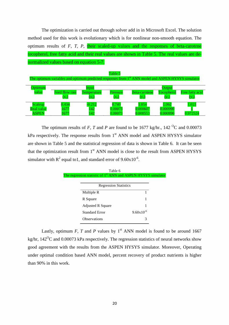
The optimization is carried out through solver add in in Microsoft Excel. The solution

method used for this work is evolutionary which is for nonlinear non-smooth equation. The

optimum results of F, T, P, their scaled-up values and the responses of beta-carotene

tocopherol, free fatty acid and their real values are shown in Table 5. The real values are de-

normalized values based on equation 5-7.

Table 5

The optimum variables and optimum predicted responses from 1st ANN model and ASPEN HYSYS simulator

Optimum

value

Input Output

Feed flow rate

(x1)

Temperature

(x2)

Pressure

(x3)

Beta-carotene

(y1)

Tocopherol

(y2)

Free fatty acid

(y3)

Scaleup 0.434 -0.212 0.749 1.054 1.062 1.023

Real value 1677 142 0.00073 0.000607 0.000990 1

ASPEN 1677 142 0.00073 0.000553 0.000896 0.972524

The optimum results of F, T and P are found to be 1677 kg/hr., 142 OC and 0.00073

kPa respectively. The response results from 1st ANN model and ASPEN HYSYS simulator

are shown in Table 5 and the statistical regression of data is shown in Table 6. It can be seen

that the optimization result from 1st ANN model is close to the result from ASPEN HYSYS

simulator with R2 equal to1, and standard error of 9.60x10

-6.

Table 6

The regression statistic of 1st ANN and ASPEN HYSYS simulator

Regression Statistics

Multiple R 1

R Square 1

Adjusted R Square 1

Standard Error 9.60x10-6

Observations 3

Lastly, optimum F, T and P values by 1st ANN model is found to be around 1667

kg/hr, 142OC and 0.00073 kPa respectively. The regression statistics of neural networks show

good agreement with the results from the ASPEN HYSYS simulator. Moreover, Operating

under optimal condition based ANN model, percent recovery of product nutrients is higher

than 90% in this work.

21

5. Conclusion

Two Neural networks based correlations for refined palm oil process to predict the

concentration of beta-carotene, tocopherol and FFA are developed. Feed forward back

propagation is used to determine the optimum architecture for the 1st ANN model (based on 3

inputs: F, T and P) and the 2nd

ANN model (based on 2 inputs: T and P). The effect of

number of layers and neurons are studied for both models. It is found that 2 layers and 20

neurons are optimum of ANN structures for both ANN models. Tansig and purelin are the

best predicted transfer function for these neural network architectures. The proposed ANN

models are capable of predicting the concentrations of beta-carotene, tocopherol and free

fatty acid very close to those obtained by ASPEN HYSYS simulator. It is found that

increasing temperature leads to decrease quality of edible oil however, increasing pressure

leads to increase the quality of edible oil.

In addition, optimizations based on optimum ANN model is performed, and the

results show that the optimum F, T and P are at 1677 kg/hr., 142OC and 0.00073 kPa

respectively. Lastly it can be concluded that ANN can be successfully applied for refined

palm oil process with a very good accuracy.

Acknowledgement

The authors would like to acknowledge the Prince of Songkla Universit, Songkhla,

Thailand for providing financial support to Mrs. Noree Tehlah for carrying out this research

abroad and the School of Engineering, University of Bradford, UK for providing research

facilities and facilitators, which make this complete and successful study.

22

References

1. Li, Y. and S.-L. Xu, DSMC simulation of vapor flow in molecular distillation. Vacuum, 2014.

110: p. 40-46.

2. Jung, J., et al., Optimal operation strategy of batch vacuum distillation for sulfuric acid

recycling process. Computers & Chemical Engineering, 2014. 71: p. 104-115.

3. Huang, H.-J., et al., A review of separation technologies in current and future biorefineries.

Separation and Purification Technology, 2008. 62(1): p. 1-21.

4. Casilio, D., N. T. Dunford. Nutritionally enhanced edible oil and oilseed processing. 178-192

Canada, AOCS Press., 2004.

5. Wang, A., et al., Process optimization for vacuum distillation of Snโ€“Sb alloy by response

surface methodology. Vacuum, 2014. 109: p. 127-134.

6. Chen, F., et al., Optimizing conditions for the purification of crude octacosanol extract from

rice bran wax by molecular distillation analyzed using response surface methodology. Journal

of Food Engineering, 2005. 70(1): p. 47-53.

7. Shao, P., S.T. Jiang, and Y.J. Ying, Optimization of Molecular Distillation for Recovery of

Tocopherol from Rapeseed Oil Deodorizer Distillate Using Response Surface and Artificial

Neural Network Models. Food and Bioproducts Processing, 2007. 85(2): p. 85-92.

8. Wu, W., C. Wang, and J. Zheng, Optimization of deacidification of low-calorie cocoa butter

by molecular distillation. LWT - Food Science and Technology, 2012. 46(2): p. 563-570.

9. Mallmann, E.S., et al., Development of a Computational Tool for Simulating Falling Film

Molecular Design. Computer Aided Chemical Engineering, 2009. 26: p. 743-748.

10. Tehlah.N, Simulation of Refined Palm Oil Process by ASPEN HYSYS, Technical Report.,

Prince of Songkla University, 2015.

11. Unnikrishnan, R., Refining of edible oil rich in natural carotenes and vitamin E., in United

State Patent 2001.

12. Motlaghi, S., F. Jalali, and M.N. Ahmadabadi, An expert system design for a crude oil

distillation column with the neural networks model and the process optimization using genetic

algorithm framework. Expert Systems with Applications, 2008. 35(4): p. 1540-1545.

13. Lluvia M., O.-E., M. Jobson, and R. Smith, Operational optimization of crude oil distillation

systems using artificial neural networks. Computer & Chemical Engineering 2013. 59: p.

178-185.

14. Osuolale, F.N., et al., Multi-objective Optimisation of Atmospheric Crude Distillation System

Operations Based on Bootstrap Aggregated Neural Network Models. Computer Aided

Chemical Engineering, 2015. Volume 37: p. 671-676.

15. Zereshki, S., Distialltion - Advances from Modeling to Application. 2012: InTech.

16. Mujtaba, I.M., A. Hussain, Application of Neural Networks and Other Learning Technologies

in Process Engineering: Imperial College Press, 2001.

17. Hagan, M.T., H.B. Demuth, and M.H. Beale, Neural Network Design. 1996: PWS Publishing

Company of international Thomson Publishing Inc., Boston.

18. Tanvir, M.S. and I.M. Mujtaba, Neural network based correlations for estimating

temperature elevation for seawater in MSF desalination process. Desalination, 2006. 195: p.

251-272.

19. Barello, M., et al., Neural network based correlation for estimating water permeability

constant in RO desalination process under fouling. Desalination, 2014. 345: p. 101-111.

20. Mashaly, A.F., et al., Predictive model for assessing and optimizing solar still performance

using artificial neural network under hyper arid environment. Solar Energy, 2015. 118: p. 41-

58.

21. Khayet, M. and C. Cojocaru, Artificial neural network modeling and optimization of

desalination by air gap membrane distillation. Separation and Purification Technology, 2012.

86: p. 171-182.

23

1. Li, Y. and S.-L. Xu, DSMC simulation of vapor flow in molecular distillation. Vacuum, 2014.

110: p. 40-46.

2. Jung, J., et al., Optimal operation strategy of batch vacuum distillation for sulfuric acid

recycling process. Computers & Chemical Engineering, 2014. 71: p. 104-115.

3. Huang, H.-J., et al., A review of separation technologies in current and future biorefineries.

Separation and Purification Technology, 2008. 62(1): p. 1-21.

4. Casilio, D., N. T. Dunford. Nutritionally enhanced edible oil and oilseed processing. 178-192

Canada, AOCS Press., 2004.

5. Wang, A., et al., Process optimization for vacuum distillation of Snโ€“Sb alloy by response

surface methodology. Vacuum, 2014. 109: p. 127-134.

6. Chen, F., et al., Optimizing conditions for the purification of crude octacosanol extract from

rice bran wax by molecular distillation analyzed using response surface methodology. Journal

of Food Engineering, 2005. 70(1): p. 47-53.

7. Shao, P., S.T. Jiang, and Y.J. Ying, Optimization of Molecular Distillation for Recovery of

Tocopherol from Rapeseed Oil Deodorizer Distillate Using Response Surface and Artificial

Neural Network Models. Food and Bioproducts Processing, 2007. 85(2): p. 85-92.

8. Wu, W., C. Wang, and J. Zheng, Optimization of deacidification of low-calorie cocoa butter

by molecular distillation. LWT - Food Science and Technology, 2012. 46(2): p. 563-570.

9. Mallmann, E.S., et al., Development of a Computational Tool for Simulating Falling Film

Molecular Design. Computer Aided Chemical Engineering, 2009. 26: p. 743-748.

10. Tehlah.N, Simulation of Refined Palm Oil Process by ASPEN HYSYS, Technical Report.,

Prince of Songkla University, 2015.

11. Unnikrishnan, R., Refining of edible oil rich in natural carotenes and vitamin E., in United

State Patent 2001.

12. Motlaghi, S., F. Jalali, and M.N. Ahmadabadi, An expert system design for a crude oil

distillation column with the neural networks model and the process optimization using genetic

algorithm framework. Expert Systems with Applications, 2008. 35(4): p. 1540-1545.

13. Lluvia M., O.-E., M. Jobson, and R. Smith, Operational optimization of crude oil distillation

systems using artificial neural networks. Computer & Chemical Engineering 2013. 59: p.

178-185.

14. Osuolale, F.N., et al., Multi-objective Optimisation of Atmospheric Crude Distillation System

Operations Based on Bootstrap Aggregated Neural Network Models. Computer Aided

Chemical Engineering, 2015. Volume 37: p. 671-676.

15. Zereshki, S., Distialltion - Advances from Modeling to Application. 2012: InTech.

16. Mujtaba, I.M., A. Hussain, Application of Neural Networks and Other Learning Technologies

in Process Engineering: Imperial College Press, 2001.

17. Hagan, M.T., H.B. Demuth, and M.H. Beale, Neural Network Design. 1996: PWS Publishing

Company of international Thomson Publishing Inc., Boston.

18. Tanvir, M.S. and I.M. Mujtaba, Neural network based correlations for estimating

temperature elevation for seawater in MSF desalination process. Desalination, 2006. 195: p.

251-272.

19. Barello, M., et al., Neural network based correlation for estimating water permeability

constant in RO desalination process under fouling. Desalination, 2014. 345: p. 101-111.

20. Mashaly, A.F., et al., Predictive model for assessing and optimizing solar still performance

using artificial neural network under hyper arid environment. Solar Energy, 2015. 118: p. 41-

58.

21. Khayet, M. and C. Cojocaru, Artificial neural network modeling and optimization of

desalination by air gap membrane distillation. Separation and Purification Technology, 2012.

86: p. 171-182.

24

Noree Tehlah received the B.Sc. degree in chemical engineering from

Universiti Teknologi Petronas (UTP), in Perak Malaysia in 2010. She is

currently studying for combined degree of Master and PhD in chemical

engineering at Prince of Songkla University (PSU), Thailand. Her current

research interests include simulation, neural network and process control.

Pornsiri Kaewpradit, Asst. Prof. Dr. is Lecturer in Department of

Chemical Engineering at Prince of Songkla University, Songkhla

THAILAND. She got her Doctoral degrees in Chemical Engineering from

Chulalongkorn University, financial supported by Royal Golden Jubilee

(RGJ), The Thailand Research Fund (TRF). Her research area is on

MODEL PREDICTIVE CONTROL (MPC) design, Mathematical and

ANN modeling, Optimization and Process simulation through MATLAB

and ASPEN/HYSYS, especially in Rubber and Energy Industries.

Iqbal M. Mujtaba is a Professor of Computational Process Engineering in the School of

Engineering, at the University of Bradford. He obtained his BSc Eng and MSc Eng degrees in

Chemical Engineering from Bangladesh University of Engineering & Technology (BUET) in 1983

and 1984 respectively and obtained his PhD from Imperial College London in 1989. He is a Fellow of

the IChemE, a Chartered Chemical Engineer, and the Chair of the IChemE's Computer Aided Process

Engineering Subject Group. Professor Mujtaba leads research into dynamic modelling, simulation,

optimisation and control of batch and continuous chemical processes with specific interests in

distillation, industrial reactors, refinery processes, desalination and crude oil hydrotreating focusing

on energy and water. He has managed several research collaborations and consultancy projects with

industry and academic institutions in the UK, Italy, Hungary, Libya, Malaysia, Thailand, Iraq and

Saudi Arabia. He has published over 230 technical papers and has delivered more than 60 invited

keynotes/lectures/seminars/short courses around the world. He has supervised 24 PhD students to

completion and is currently supervising 10 PhD students. He is the author of 'Batch Distillation:

Design & Operation' (text book) published by the Imperial College Press, London, 2004 which is

based on his 18 years of research in Batch Distillation.

25

26

APPENDIX

Table A

Weights, bias and transfer function of neural network (20 neurons) (1st ANN model)

Weights

1st layer

Weight size for 1st layer [20x3] Bias size [20x1]

Transfer

function

𝑤1,11 = -2.340 𝑤21

1 = 7.202 𝑤3,11 = 8.285 𝐵1

1 -12.892 𝑓11 = 𝑡𝑎𝑛ℎ

𝑤1,21 = 3.119 𝑤2,2

1 = 6.517 𝑤3,21 = -1.800 𝐵2

1 -5.737 𝑓21 = 𝑡𝑎𝑛ℎ

𝑤1,31 = -0.109 𝑤2,3

1 = 1.819 𝑤3,31 = -5.171 𝐵3

1 -2.627 𝑓31 = 𝑡𝑎𝑛ℎ

𝑤1,41 = 0.091 𝑤2,4

1 = -2.655 𝑤3,41 = 3.740 𝐵4

1 2.952 𝑓41 = 𝑡𝑎𝑛ℎ

𝑤1,51 = 1.240 𝑤2,5

1 = 0.462 𝑤3,51 = -0.086 𝐵5

1 -0.398 𝑓51 = 𝑡𝑎𝑛ℎ

𝑤1,61 = 7.711 𝑤2,6

1 = -4.299 𝑤3,61 = 9.855 𝐵6

1 -4.618 𝑓61 = 𝑡𝑎𝑛ℎ

𝑤1,71 = 4.056 𝑤2,7

1 = -2.964 𝑤3,71 = -4.874 𝐵7

1 0.646 𝑓71 = 𝑡𝑎𝑛ℎ

𝑤1,81 = 1.124 𝑤2,8

1 = 1.893 𝑤3,81 = 0.971 𝐵8

1 0.003 𝑓81 = 𝑡𝑎𝑛ℎ

𝑤1,91 = -0.058 𝑤2,9

1 = 2.534 𝑤3,91 = -1.215 𝐵9

1 -0.370 𝑓91 = 𝑡𝑎𝑛ℎ

𝑤1,101 = -4.128 𝑤2,10

1 = -0.295 𝑤3,101 = -0.149 𝐵10

1 -0.444 𝑓101 = 𝑡𝑎𝑛ℎ

𝑤1,111 = -6.671 𝑤2,11

1 = 2.649 𝑤3,111 = -5.390 𝐵11

1 -0.840 𝑓111 = 𝑡𝑎𝑛ℎ

𝑤1,121 = 0.022 𝑤2,12

1 = 0.867 𝑤3,121 = -3.115 𝐵12

1 -0.201 𝑓121 = 𝑡𝑎𝑛ℎ

𝑤1,131 = -0.061 𝑤2,13

1 = 2.029 𝑤3,131 = 0.009 𝐵13

1 -0.054 𝑓131 = 𝑡𝑎𝑛ℎ

𝑤1,141 = -3.183 𝑤2,14

1 = -8.906 𝑤3,141 = -1.264 𝐵14

1 -0.553 𝑓141 = 𝑡𝑎𝑛ℎ

𝑤1,151 = 3.911 𝑤2,15

1 = -1.955 𝑤3,151 = -4.045 𝐵15

1 1.653 𝑓151 = 𝑡𝑎𝑛ℎ

𝑤1,161 = -0.055 𝑤2,16

1 = 0.330 𝑤3,161 = -0.629 𝐵16

1 -1.598 𝑓161 = 𝑡𝑎𝑛ℎ

𝑤1,171 = 0.003 𝑤2,17

1 = -0.644 𝑤3,171 = -1.888 𝐵17

1 -2.442 𝑓171 = 𝑡𝑎𝑛ℎ

𝑤1,181 = 3.208 𝑤2,18

1 = 1.796 𝑤3,181 = -2.444 𝐵18

1 4.337 𝑓181 = 𝑡𝑎𝑛ℎ

𝑤1,191 = -0.087 𝑤2,19

1 = 3.662 𝑤3,191 = -1.591 𝐵19

1 -0.335 𝑓191 = 𝑡𝑎𝑛ℎ

𝑤1,201 = 0.126 𝑤2,20

1 = 1.734 𝑤3,201 = 1.405 𝐵20

1 -1.695 𝑓201 = 𝑡𝑎𝑛ℎ

Weight

2nd

layer Weight size for 2

nd layer [20x3] Bias size [3x1]

Transfer

function

𝑤1,12 = 0.070 𝑤1,2

2 = 0.040 𝑤1,32 = 0.008 𝐵1

2 -1.618 𝑓13 = 1

𝑤2,12 = 0.027 𝑤2,2

2 = 0.017 𝑤2,32 = 0.012 𝐵2

2 -1.487

𝑤3,12 = 0.347 𝑤3,2

2 = 0.417 𝑤3,32 = 0.347 𝐵3

3 -0.503

𝑤4,12 = 0.761 𝑤4,2

2 = 0.849 𝑤4,32 = 0.744

𝑤5,12 = 0.039 𝑤5,2

2 = 0.039 𝑤5,32 = 0.042

𝑤6,12 = -0.003 𝑤6,2

2 = -0.007 𝑤6,32 = -0.035

𝑤7,12 = -0.037 𝑤7,2

2 = -0.039 𝑤7,32 = -0.048

𝑤8,12 = -0.042 𝑤8,2

2 = -0.017 𝑤8,32 = 0.025

𝑤9,12 = -2.309 𝑤9,2

2 = -2.383 𝑤9,32 = -1.982

𝑤10,12 = 0.030 𝑤10,2

2 = 0.041 𝑤10,32 = 0.043

𝑤11,12 = 0.006 𝑤11,2

2 = -0.002 𝑤11,32 = -0.021

𝑤12,12 = 0.198 𝑤12,2

2 = 0.191 𝑤12,32 = 0.153

𝑤13,12 = 0.399 𝑤13,2

2 = 0.410 𝑤13,32 = 0.197

𝑤14,12 = -0.045 𝑤14,2

2 = -0.038 𝑤14,32 = -0.006

𝑤15,12 = 0.028 𝑤15,2

1 = 0.031 𝑤15,31 = 0.030

𝑤16,12 = -0.692 𝑤16,2

2 = -0.467 𝑤16,32 = 0.755

𝑤17,12 = -0.780 𝑤17,2

2 = -0.767 𝑤17,32 = -0.816

𝑤18,12 = 0.041 𝑤18,2

2 = 0.041 𝑤18,32 = 0.046

𝑤19,12 = 1.296 𝑤19,2

2 = 1.350 𝑤19,32 = 0.922

𝑤20,12 = -0.424 𝑤20,2

2 = -0.457 𝑤20,32 = -0.373

27

Table B

Weights, bias and transfer function of neural network (20 neurons) (2nd ANN model)*.

Weights

1st layer

Weight size for 1st layer [20x2] Bias size [20x1]

Transfer

function

𝑤1,11 = 3.641 𝑤21

1 = 4.651 𝐵11 -6.061 𝑓1

1 = 𝑡𝑎𝑛ℎ

𝑤1,21 = -3.367 𝑤2,2

1 = 6.123 𝐵21 5.411 𝑓2

1 = 𝑡𝑎𝑛ℎ

𝑤1,31 = -2.667 𝑤2,3

1 = 5.405 𝐵31 4.263 𝑓3

1 = 𝑡𝑎𝑛ℎ

𝑤1,41 = -2.598 𝑤2,4

1 = -5.587 𝐵41 3.939 𝑓4

1 = 𝑡𝑎𝑛ℎ

𝑤1,51 = 5.967 𝑤2,5

1 = -1.332 𝐵51 -3.678 𝑓5

1 = 𝑡𝑎𝑛ℎ

𝑤1,61 = -3.770 𝑤2,6

1 = -5.178 𝐵61 3.533 𝑓6

1 = 𝑡𝑎𝑛ℎ

𝑤1,71 = 8.412 𝑤2,7

1 = -3.426 𝐵71 -2.545 𝑓7

1 = 𝑡𝑎𝑛ℎ

𝑤1,81 = -3.650 𝑤2,8

1 = -6.020 𝐵81 1.169 𝑓8

1 = 𝑡𝑎𝑛ℎ

𝑤1,91 = 0.532 𝑤2,9

1 = -6.467 𝐵91 0.997 𝑓9

1 = 𝑡𝑎𝑛ℎ

𝑤1,101 = 5.699 𝑤2,10

1 = 1.136 𝐵101 -1.574 𝑓10

1 = 𝑡𝑎𝑛ℎ

𝑤1,111 = 3.181 𝑤2,11

1 = 4.802 𝐵111 1.013 𝑓11

1 = 𝑡𝑎𝑛ℎ

𝑤1,121 = -7.066 𝑤2,12

1 = -0.221 𝐵121 -0.206 𝑓12

1 = 𝑡𝑎𝑛ℎ

𝑤1,131 = 6.416 𝑤2,13

1 = 0.618 𝐵131 0.412 𝑓13

1 = 𝑡𝑎𝑛ℎ

𝑤1,141 = -5.754 𝑤2,14

1 = 3.587 𝐵141 -3.039 𝑓14

1 = 𝑡𝑎𝑛ℎ

𝑤1,151 = 4.747 𝑤2,15

1 = 2.643 𝐵151 3.083 𝑓15

1 = 𝑡𝑎𝑛ℎ

𝑤1,161 = 5.735 𝑤2,16

1 = -0.069 𝐵161 4.800 𝑓16

1 = 𝑡𝑎𝑛ℎ

𝑤1,171 = -0.280 𝑤2,17

1 = 6.017 𝐵171 5.153 𝑓17

1 = 𝑡𝑎𝑛ℎ

𝑤1,181 = 1.990 𝑤2,18

1 = -5.681 𝐵181 4.090 𝑓18

1 = 𝑡𝑎𝑛ℎ

𝑤1,191 = 3.572 𝑤2,19

1 = 2.182 𝐵191 5.249 𝑓19

1 = 𝑡𝑎𝑛ℎ

𝑤1,201 = -5.481 𝑤2,20

1 = -2.805 𝐵201 -7.229 𝑓20

1 = 𝑡𝑎𝑛ℎ

Weight

2nd

layer Weight size for 2

nd layer [20x3] Bias size [3x1]

Transfer

function

𝑤1,12 = 0.056 𝑤1,2

2 = 0.038 𝑤1,32 = -0.008 𝐵1

2 0.050 𝑓13 = 1

𝑤2,12 = -0.702 𝑤2,2

2 = -0.482 𝑤2,32 = -0.703 𝐵2

2 0.018

𝑤3,12 = 0.900 𝑤3,2

2 = 0.651 𝑤3,32 = 0.725 𝐵3

3 0.075

𝑤4,12 = -0.034 𝑤4,2

2 = -0.001 𝑤4,32 = -0.018

𝑤5,12 = -0.610 𝑤5,2

2 = -0.660 𝑤5,32 = -0.409

𝑤6,12 = 0.110 𝑤6,2

2 = 0.062 𝑤6,32 = 0.012

𝑤7,12 = -0.050 𝑤7,2

2 = -0.030 𝑤7,32 = -0.227

𝑤8,12 = 0.012 𝑤8,2

2 = 0.004 𝑤8,32 = 0.000

𝑤9,12 = 0.000 𝑤9,2

2 = 0.013 𝑤9,32 = 0.007

𝑤10,12 = -0.255 𝑤10,2

2 = 0.015 𝑤10,32 = -0.133

𝑤11,12 = -0.027 𝑤11,2

2 = 0.011 𝑤11,32 = 0.040

𝑤12,12 = -1.343 𝑤12,2

2 = 0.294 𝑤12,32 = 0.330

𝑤13,12 = -1.132 𝑤13,2

2 = 0.180 𝑤13,32 = 0.155

𝑤14,12 = 0.061 𝑤14,2

2 = 0.020 𝑤14,32 = 0.020

𝑤15,12 = -0.019 𝑤15,2

1 = -0.020 𝑤15,31 = -0.058

𝑤16,12 = 0.027 𝑤16,2

2 = 0.027 𝑤16,32 = -0.023

𝑤17,12 = 0.071 𝑤17,2

2 = 0.025 𝑤17,32 = -0.020

𝑤18,12 = -0.015 𝑤18,2

2 = -0.002 𝑤18,32 = 0.008

𝑤19,12 = 0.775 𝑤19,2

2 = 0.382 𝑤19,32 = 1.184

𝑤20,12 = 0.850 𝑤20,2

2 = 0.437 𝑤20,32 = 1.191

*without considering feed flow rate

28

Table C

Data used in the 1st ANN Model

No. F

(kg/hr)

T

(oC)

P

(kPa) Y1 Y2 Y3 No.

F

(kg/hr)

T

(oC)

P

(kPa) Y1 Y2 Y3

1 1000 100 0.00000 0.00052 0.00088 0.98 71 1500 125 0.00040 0.00056 0.00091 0.99

2 1000 100 0.00010 0.00056 0.00091 1.00 72 1500 125 0.00050 0.00056 0.00091 0.99

3 1000 100 0.00020 0.00056 0.00091 1.00 73 1500 125 0.00060 0.00056 0.00091 0.99

4 1000 100 0.00030 0.00056 0.00090 1.00 74 1500 125 0.00070 0.00056 0.00091 1.00

5 1000 100 0.00040 0.00056 0.00090 1.00 75 1500 125 0.00080 0.00056 0.00091 1.00 6 1000 100 0.00050 0.00056 0.00090 1.00 76 1500 125 0.00090 0.00056 0.00091 1.00

7 1000 100 0.00060 0.00055 0.00089 1.00 77 1500 125 0.00100 0.00056 0.00091 1.00

8 1000 100 0.00070 0.00055 0.00089 1.00 78 1500 150 0.00000 0.00003 0.00005 0.09

9 1000 100 0.00080 0.00055 0.00089 1.00 79 1500 150 0.00010 0.00038 0.00067 0.65

10 1000 100 0.00090 0.00055 0.00089 1.00 80 1500 150 0.00020 0.00047 0.00078 0.80

11 1000 100 0.00100 0.00055 0.00089 1.00 81 1500 150 0.00030 0.00050 0.00083 0.86

12 1000 125 0.00000 0.00031 0.00062 0.73 82 1500 150 0.00040 0.00052 0.00085 0.89

13 1000 125 0.00010 0.00053 0.00088 0.97 83 1500 150 0.00050 0.00053 0.00086 0.91

14 1000 125 0.00020 0.00055 0.00090 0.98 84 1500 150 0.00060 0.00053 0.00087 0.93

15 1000 125 0.00030 0.00056 0.00090 0.99 85 1500 150 0.00070 0.00054 0.00088 0.94

16 1000 125 0.00040 0.00056 0.00091 0.99 86 1500 150 0.00080 0.00054 0.00088 0.95

17 1000 125 0.00050 0.00056 0.00091 0.99 87 1500 150 0.00090 0.00055 0.00089 0.95

18 1000 125 0.00060 0.00056 0.00091 0.99 88 1500 150 0.00100 0.00055 0.00089 0.96

19 1000 125 0.00070 0.00056 0.00091 1.00 89 1500 175 0.00000 0.00000 0.00001 0.07

20 1000 125 0.00080 0.00056 0.00091 1.00 90 1500 175 0.00010 0.00000 0.00001 0.07

21 1000 125 0.00090 0.00056 0.00091 1.00 91 1500 175 0.00020 0.00017 0.00027 0.18

22 1000 125 0.00100 0.00056 0.00091 1.00 92 1500 175 0.00030 0.00027 0.00043 0.29

23 1000 150 0.00000 0.00003 0.00005 0.09 93 1500 175 0.00040 0.00033 0.00054 0.38

24 1000 150 0.00010 0.00038 0.00067 0.65 94 1500 175 0.00050 0.00038 0.00061 0.46

25 1000 150 0.00020 0.00047 0.00078 0.80 95 1500 175 0.00060 0.00041 0.00065 0.52

26 1000 150 0.00030 0.00050 0.00083 0.86 96 1500 175 0.00070 0.00043 0.00069 0.56

27 1000 150 0.00040 0.00052 0.00085 0.89 97 1500 175 0.00080 0.00045 0.00072 0.60

28 1000 150 0.00050 0.00053 0.00086 0.91 98 1500 175 0.00090 0.00046 0.00074 0.64 29 1000 150 0.00060 0.00053 0.00087 0.93 99 1500 175 0.00100 0.00047 0.00076 0.66

30 1000 150 0.00070 0.00054 0.00088 0.94 100 1500 200 0.00000 0.00000 0.00000 0.06

31 1000 150 0.00080 0.00054 0.00088 0.95 101 1500 200 0.00010 0.00001 0.00002 0.07

32 1000 150 0.00090 0.00055 0.00089 0.95 102 1500 200 0.00020 0.00003 0.00003 0.07

33 1000 150 0.00100 0.00055 0.00089 0.96 103 1500 200 0.00030 0.00004 0.00005 0.08

34 1000 175 0.00000 0.00000 0.00001 0.07 104 1500 200 0.00040 0.00006 0.00007 0.08

35 1000 175 0.00010 0.00000 0.00001 0.07 105 1500 200 0.00050 0.00007 0.00010 0.08

36 1000 175 0.00020 0.00017 0.00027 0.18 106 1500 200 0.00060 0.00009 0.00012 0.09

37 1000 175 0.00030 0.00027 0.00043 0.29 107 1500 200 0.00070 0.00011 0.00014 0.10 38 1000 175 0.00040 0.00033 0.00054 0.38 108 1500 200 0.00080 0.00013 0.00017 0.10

39 1000 175 0.00050 0.00038 0.00061 0.46 109 1500 200 0.00090 0.00015 0.00020 0.11

40 1000 175 0.00060 0.00041 0.00065 0.52 110 1500 200 0.00100 0.00017 0.00023 0.12 41 1000 175 0.00070 0.00043 0.00069 0.56 111 2000 100 0.00000 0.00052 0.00088 0.98

42 1000 175 0.00080 0.00045 0.00072 0.60 112 2000 100 0.00010 0.00056 0.00091 1.00

43 1000 175 0.00090 0.00046 0.00074 0.64 113 2000 100 0.00020 0.00056 0.00091 1.00

44 1000 175 0.00100 0.00047 0.00076 0.66 114 2000 100 0.00030 0.00056 0.00090 1.00

45 1000 200 0.00000 0.00000 0.00000 0.06 115 2000 100 0.00040 0.00056 0.00090 1.00

46 1000 200 0.00010 0.00001 0.00002 0.07 116 2000 100 0.00050 0.00056 0.00090 1.00

47 1000 200 0.00020 0.00003 0.00003 0.07 117 2000 100 0.00060 0.00055 0.00089 1.00

48 1000 200 0.00030 0.00004 0.00005 0.08 118 2000 100 0.00070 0.00055 0.00089 1.00

49 1000 200 0.00040 0.00006 0.00007 0.08 119 2000 100 0.00080 0.00055 0.00089 1.00 50 1000 200 0.00050 0.00007 0.00010 0.08 120 2000 100 0.00090 0.00055 0.00089 1.00

51 1000 200 0.00060 0.00009 0.00012 0.09 121 2000 100 0.00100 0.00055 0.00089 1.00

52 1000 200 0.00070 0.00011 0.00014 0.10 122 2000 125 0.00000 0.00031 0.00062 0.73

53 1000 200 0.00080 0.00013 0.00017 0.10 123 2000 125 0.00010 0.00053 0.00088 0.97

54 1000 200 0.00090 0.00015 0.00020 0.11 124 2000 125 0.00020 0.00055 0.00090 0.98

55 1000 200 0.00100 0.00017 0.00023 0.12 125 2000 125 0.00030 0.00056 0.00090 0.99

56 1500 100 0.00000 0.00052 0.00088 0.98 126 2000 125 0.00040 0.00056 0.00091 0.99

57 1500 100 0.00010 0.00056 0.00091 1.00 127 2000 125 0.00050 0.00056 0.00091 0.99

58 1500 100 0.00020 0.00056 0.00091 1.00 128 2000 125 0.00060 0.00056 0.00091 0.99

59 1500 100 0.00030 0.00056 0.00090 1.00 129 2000 125 0.00070 0.00056 0.00091 1.00

60 1500 100 0.00040 0.00056 0.00090 1.00 130 2000 125 0.00080 0.00056 0.00091 1.00

61 1500 100 0.00050 0.00056 0.00090 1.00 131 2000 125 0.00090 0.00056 0.00091 1.00 62 1500 100 0.00060 0.00055 0.00089 1.00 132 2000 125 0.00100 0.00056 0.00091 1.00

63 1500 100 0.00070 0.00055 0.00089 1.00 133 2000 150 0.00000 0.00003 0.00005 0.09

64 1500 100 0.00080 0.00055 0.00089 1.00 134 2000 150 0.00010 0.00038 0.00067 0.65

65 1500 100 0.00090 0.00055 0.00089 1.00 135 2000 150 0.00020 0.00047 0.00078 0.80

66 1500 100 0.00100 0.00055 0.00089 1.00 136 2000 150 0.00030 0.00050 0.00083 0.86

67 1500 125 0.00000 0.00031 0.00062 0.73 137 2000 150 0.00040 0.00052 0.00085 0.89

68 1500 125 0.00010 0.00053 0.00088 0.97 138 2000 150 0.00050 0.00053 0.00086 0.91

69 1500 125 0.00020 0.00055 0.00090 0.98 139 2000 150 0.00060 0.00053 0.00087 0.93

70 1500 125 0.00030 0.00056 0.00090 0.99 140 2000 150 0.00070 0.00054 0.00088 0.94

29

Table 1 cont’d

No. F

(kg/hr) T (oC)

P (kPa)

Y1 Y2 Y3 No. F

(kg/hr) T

(oC) P

(kPa) Y1 Y2 Y3

141 2000 150 0.00080 0.00054 0.00088 0.95 154 2000 175 0.00100 0.00046 0.00074 0.64 142 2000 150 0.00090 0.00055 0.00089 0.95 155 2000 200 0.00000 0.00047 0.00076 0.66 143 2000 150 0.00100 0.00055 0.00089 0.96 156 2000 200 0.00010 0.00000 0.00000 0.06 144 2000 175 0.00000 0.00000 0.00001 0.07 157 2000 200 0.00020 0.00001 0.00002 0.07 145 2000 175 0.00010 0.00000 0.00001 0.07 158 2000 200 0.00030 0.00003 0.00003 0.07 146 2000 175 0.00020 0.00017 0.00027 0.18 159 2000 200 0.00040 0.00004 0.00005 0.08 147 2000 175 0.00030 0.00027 0.00043 0.29 160 2000 200 0.00050 0.00006 0.00007 0.08 148 2000 175 0.00040 0.00033 0.00054 0.38 161 2000 200 0.00060 0.00007 0.00010 0.08 149 2000 175 0.00050 0.00038 0.00061 0.46 162 2000 200 0.00070 0.00009 0.00012 0.09 150 2000 175 0.00060 0.00041 0.00065 0.52 163 2000 200 0.00080 0.00011 0.00014 0.10 151 2000 175 0.00070 0.00043 0.00069 0.56 164 2000 200 0.00090 0.00013 0.00017 0.10 152 2000 175 0.00080 0.00045 0.00072 0.60 165 2000 200 0.00100 0.00015 0.00020 0.11

153 2000 175 0.00090 0.00054 0.00088 0.95

Note: Bold data for Training, Italic data for Validation, Plain data in Test.