The Two-dimensional Navier-Stokes Equationsand the Oseen Vortex

C. E. Wayne

March 18, 2014

IMPA Vortices, L.1

Abstract

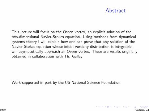
This lecture will focus on the Oseen vortex, an explicit solution of thetwo-dimensional Navier-Stokes equation. Using methods from dynamicalsystems theory I will explain how one can prove that any solution of theNavier-Stokes equation whose initial vorticity distribution is integrablewill asymptotically approach an Oseen vortex. These are results originallyobtained in collaboration with Th. Gallay

Work supported in part by the US National Science Foundation.

IMPA Vortices, L.1

Introduction

1 Understanding the long-time evolution of fluid motion is oftenfacilitated by studying the coherent structures of the flow.

2 In physical flows, these structures are often vortices.

3 From a mathematical point of view these structures may beinvariant manifolds in the phase space of the system.

IMPA Vortices, L.1

Two-dimensional fluids

1 Although we live in a three dimensional world, many fluid flowsbehave in an essentially two-dimensional way.

(a) In many physical circumstances (e.g. the ocean or theatmosphere), one dimensional of the domain is much smallerthan either the other two dimensions, or the dimensions oftypical features of interest.

(b) This effect is compounded by the effects of stratification androtation.

2 There are fascinating physical and mathematical differences betweentwo and three dimensional flows.

IMPA Vortices, L.1

Two-dimensional fluids

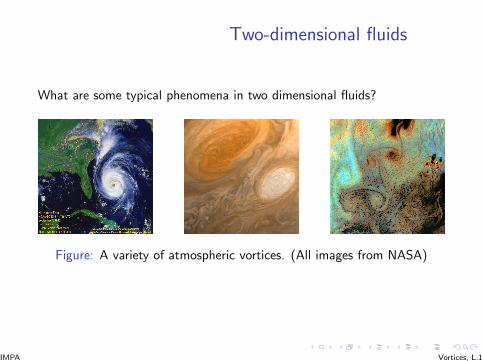
What are some typical phenomena in two dimensional fluids?

Figure: A variety of atmospheric vortices. (All images from NASA)

IMPA Vortices, L.1

Two-dimensional vortices

One of the characteristic features of two-dimensional flows is thetendency of large vortices to form regardless of the initial state of thefluid.

• This is in marked contrast to three-dimensional fluids where energyflows from large scales to small scales.

• This is an example of the “inverse cascade” of energy intwo-dimensional fluids.

How do we characterize vortices?

IMPA Vortices, L.1

The Navier-Stokes Equations

A system of nonlinear partial differential equations which describe themotion of a viscous, incompressible fluid.

If u(x , t) describes the velocity of the fluid at the point x and time t thenthe evolution of u is described by:

∂u

∂t+ (u · ∇)u = ν∆u−∇p , ∇ · u = 0 ,

The first of these equations is basically Newton’s Law; F = ma while thesecond just enforces the fact that the fluid is incompressible.

IMPA Vortices, L.1

Vorticity

The velocity of the fluid is not the best way to visualize or characterizevortices, however, for that it is better to use the vorticity!

Roughly speaking, the vorticity describes how much “swirl” there is inthe fluid.

ω(x , t) = ∇× u(x , t)

Note that for two-dimensional fluid flows, u(x , t) = (u1(x , y), u2(x , y), 0),so

ω = ∇× u = (0, 0, ∂xu2 − ∂yu1) .

Note that in two dimensions we can treat the vorticity as a scalar!

IMPA Vortices, L.1

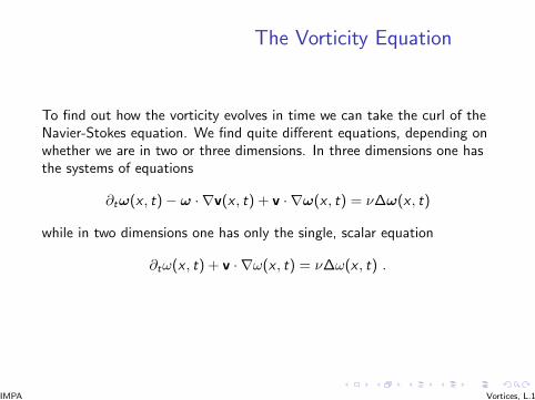
The Vorticity Equation

To find out how the vorticity evolves in time we can take the curl of theNavier-Stokes equation. We find quite different equations, depending onwhether we are in two or three dimensions. In three dimensions one hasthe systems of equations

∂tω(x , t)− ω · ∇v(x , t) + v · ∇ω(x , t) = ν∆ω(x , t)

while in two dimensions one has only the single, scalar equation

∂tω(x , t) + v · ∇ω(x , t) = ν∆ω(x , t) .

IMPA Vortices, L.1

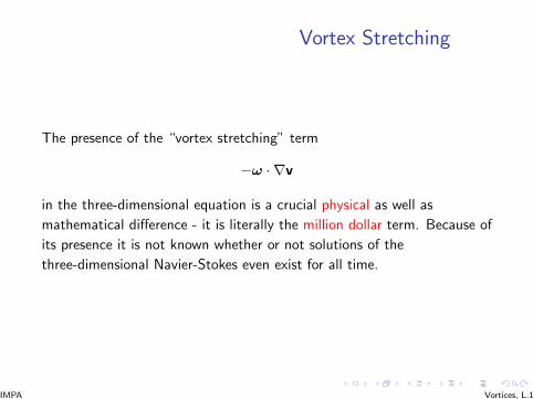
Vortex Stretching

The presence of the “vortex stretching” term

−ω · ∇v

in the three-dimensional equation is a crucial physical as well as

mathematical difference - it is literally the million dollar term. Because of

its presence it is not known whether or not solutions of the

three-dimensional Navier-Stokes even exist for all time.

IMPA Vortices, L.1

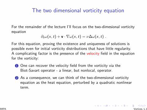
The two dimensional vorticity equation

For the remainder of the lecture I’ll focus on the two-dimesional vorticityequation

∂tω(x , t) + v · ∇ω(x , t) = ν∆ω(x , t) .

For this equation, proving the existence and uniqueness of solutions ispossible even for initial vorticity distributions that have little regularity.A complicating factor is the presence of the velocity field in the equationfor the vorticity:

1 One can recover the velocity field from the vorticity via theBiot-Savart operator - a linear, but nonlocal, operator.

2 As a consequence, we can think of the two-dimensional vorticityequation as the heat equation, perturbed by a quadratic nonlinearterm.

IMPA Vortices, L.1

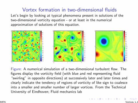
Vortex formation in two-dimensional fluidsLet’s begin by looking at typical phenomena present in solutions of thetwo-dimensional vorticity equation - or at least in the numericalapproximation of solutions of this equation.

Figure: A numerical simulation of a two-dimensional turbulent flow. Thefigures display the vorticity field (with blue and red representing fluid“swirling” in opposite directions) at successively later and later times andclearly indicate the tendency of regions of vorticity of like sign to coalesceinto a smaller and smaller number of larger vortices. From the TechnicalUniversity of Eindhoven; Fluid mechanics lab

IMPA Vortices, L.1

Emergence of Vortices

Our goal will be to try and understand the emergence and stability ofthese large vortices from very general initial conditions fortwo-dimensional flows – – or more poetically,

When little whirls meet little whirls,they show a strong affection;elope, or form a bigger whirl,and so on by advection.

This is quoted without attribution onhttp://www.fluid.tue.nl/WDY/vort/2Dturb/2Dturb.html

IMPA Vortices, L.1

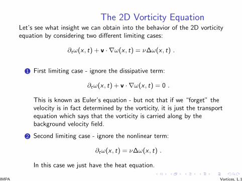
The 2D Vorticity EquationLet’s see what insight we can obtain into the behavior of the 2D vorticityequation by considering two different limiting cases:

∂tω(x , t) + v · ∇ω(x , t) = ν∆ω(x , t) .

1 First limiting case - ignore the dissipative term:

∂tω(x , t) + v · ∇ω(x , t) = 0 .

This is known as Euler’s equation - but not that if we “forget” thevelocity is in fact determined by the vorticity, it is just the transportequation which says that the vorticity is carried along by thebackground velocity field.

2 Second limiting case - ignore the nonlinear term:

∂tω(x , t) = ν∆ω(x , t) .

In this case we just have the heat equation.

IMPA Vortices, L.1

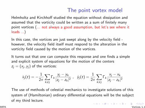
The point vortex modelHelmholtz and Kirchhoff studied the equation without dissipation andassumed that the vorticity could be written as a sum of finitely manypoint vortices (... not always a good assumption, but let’s see where itleads ...)

In this case, the vortices are just swept along by the velocity field -however, the velocity field itself must respond to the alteration in thevorticity field caused by the motion of the vortices.

It turns out that one can compute this response and one finds a simpleand explicit system of equations for the motion of the centerszj = (xj , yj) of the vortices:

xj(t) = − 1

2π

∑k 6=j

Γkyj − yk|zj − zk |2

, yj(t) =1

2π

∑k 6=j

Γkxj − xk|zj − zk |2

The use of methods of celestial mechanics to investigate solutions of this

system of (Hamiltonian) ordinary differential equations will be the subject

of my third lecture.

IMPA Vortices, L.1

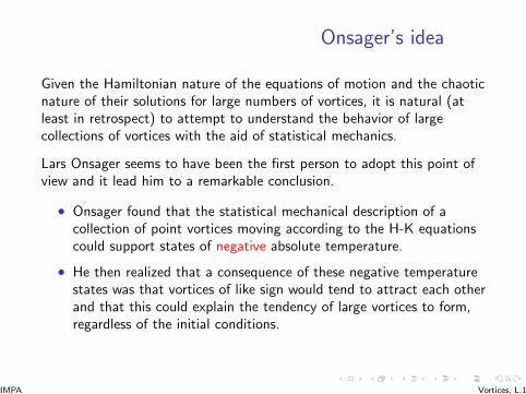
Onsager’s idea

Given the Hamiltonian nature of the equations of motion and the chaoticnature of their solutions for large numbers of vortices, it is natural (atleast in retrospect) to attempt to understand the behavior of largecollections of vortices with the aid of statistical mechanics.

Lars Onsager seems to have been the first person to adopt this point ofview and it lead him to a remarkable conclusion.

• Onsager found that the statistical mechanical description of acollection of point vortices moving according to the H-K equationscould support states of negative absolute temperature.

• He then realized that a consequence of these negative temperaturestates was that vortices of like sign would tend to attract each otherand that this could explain the tendency of large vortices to form,regardless of the initial conditions.

IMPA Vortices, L.1

Drawbacks

The limitation of Onsager’s idea is that even now, sixty years afterOnsager first proposed this method of explaining the formation of largevortices, we have no idea of whether or not the hypotheses that underlythe theory of statistical mechanics are actually satisfied by the dynamicalsystem defined by the H-K equations.

IMPA Vortices, L.1

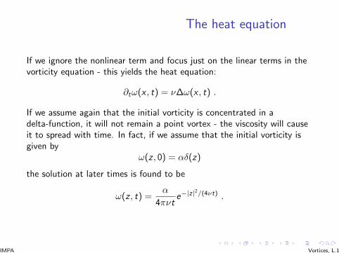
The heat equation

If we ignore the nonlinear term and focus just on the linear terms in thevorticity equation - this yields the heat equation:

∂tω(x , t) = ν∆ω(x , t) .

If we assume again that the initial vorticity is concentrated in adelta-function, it will not remain a point vortex - the viscosity will causeit to spread with time. In fact, if we assume that the initial vorticity isgiven by

ω(z , 0) = αδ(z)

the solution at later times is found to be

ω(z , t) =α

4πνte−|z|

2/(4νt) .

IMPA Vortices, L.1

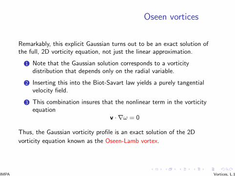
Oseen vortices

Remarkably, this explicit Gaussian turns out to be an exact solution ofthe full, 2D vorticity equation, not just the linear approximation.

1 Note that the Gaussian solution corresponds to a vorticitydistribution that depends only on the radial variable.

2 Inserting this into the Biot-Savart law yields a purely tangentialvelocity field.

3 This combination insures that the nonlinear term in the vorticityequation

v · ∇ω = 0

Thus, the Gaussian vorticity profile is an exact solution of the 2D

vorticity equation known as the Oseen-Lamb vortex.

IMPA Vortices, L.1

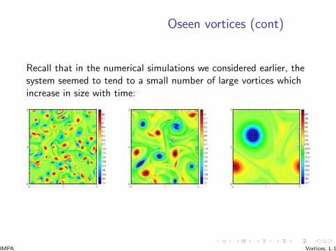
Oseen vortices (cont)

Recall that in the numerical simulations we considered earlier, thesystem seemed to tend to a small number of large vortices whichincrease in size with time:

IMPA Vortices, L.1

Scaling variables

Note that the formula for the Oseen vortices shows that the size of thevortex increases with time (like

√t ). This is consistent with the

simulations we looked at above and suggests that the analysis of thesevortices may be more natural in rescaled coordinates. With this in mindwe introduce “scaling variables” or “similarity variables”:

ξ =x√

1 + t, τ = log(1 + t) .

IMPA Vortices, L.1

Scaling variables (cont.)

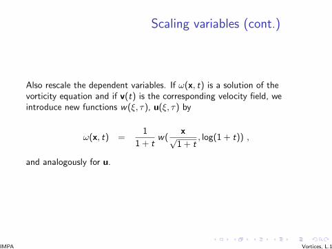
Also rescale the dependent variables. If ω(x, t) is a solution of thevorticity equation and if v(t) is the corresponding velocity field, weintroduce new functions w(ξ, τ), u(ξ, τ) by

ω(x, t) =1

1 + tw(

x√1 + t

, log(1 + t)) ,

and analogously for u.

IMPA Vortices, L.1

Scaling variables (cont.)

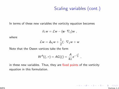
In terms of these new variables the vorticity equation becomes

∂τw = Lw − (u · ∇ξ)w ,

where

Lw = ∆ξw +1

2ξ · ∇ξw + w

Note that the Oseen vortices take the form

W A(ξ, τ) = AG (ξ) =A

4πe−

ξ2

4 ,

in these new variables. Thus, they are fixed points of the vorticity

equation in this formulation.

IMPA Vortices, L.1

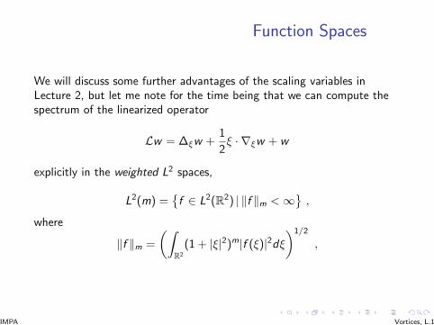
Function Spaces

We will discuss some further advantages of the scaling variables inLecture 2, but let me note for the time being that we can compute thespectrum of the linearized operator

Lw = ∆ξw +1

2ξ · ∇ξw + w

explicitly in the weighted L2 spaces,

L2(m) ={f ∈ L2(R2) | ‖f ‖m <∞

},

where

‖f ‖m =

(∫R2

(1 + |ξ|2)m|f (ξ)|2dξ)1/2

,

IMPA Vortices, L.1

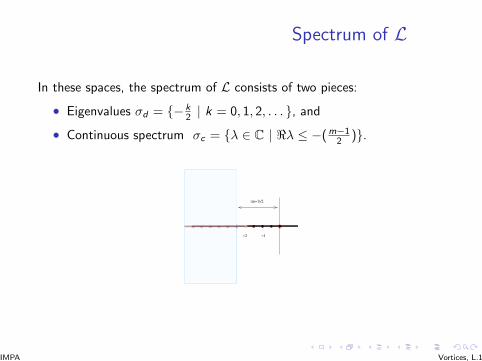
Spectrum of L

In these spaces, the spectrum of L consists of two pieces:

• Eigenvalues σd = {− k2 | k = 0, 1, 2, . . . }, and

• Continuous spectrum σc = {λ ∈ C | <λ ≤ −(m−12 )}.

� �� �� �� ����

�����

� �� �� �� ���

����

� �� �� �� � � �

� �� �� � � �

� �� �� � �

���

� � � � � � � � � � � �� � � � � � � � � � � �(m−1)/2

−1−2

IMPA Vortices, L.1

Spectrum of L

In these spaces, the spectrum of L consists of two pieces:

• Eigenvalues σd = {− k2 | k = 0, 1, 2, . . . }, and

• Continuous spectrum σc = {λ ∈ C | <λ ≤ −(m−12 )}.

� �� �� �� ���������� �� �

� �� ������� � �� �� �� � � �� �

� �� � � �� �� �� � ����

� � � � � � � � � � � �� � � � � � � � � � � �(m−1)/2

−1−2

IMPA Vortices, L.1

Dynamical Systems

It is natural to inquire whether or not these fixed points are stable. Itturns out (somewhat remarkably) that they are actually globally stable.Any solution of the two-dimensional vorticity equation whose initialvelocity is integrable will approach one of these Oseen vortices.

There are (at least) two approaches that we could use to study thestability of these vortex solutions:

• A local approach, based linearization about the fixed point.

• A global approach based on Lyapunov functionals.

IMPA Vortices, L.1

Global Stability

Recall that a Lyapunov function is a function that decreases alongsolutions of our dynamical system. In the present case it will be afunctional of the vorticity field w(ξ, τ) which is monotonic non-increasingas a function of time.

We’ll look for the ω-limit set of solutions of the 2D vorticity equation.

1 Describes the long-time behavior of solutions.

2 Can be a fixed point, periodic orbit, or even a chaotic attractor.

3 Always exists provided the system satisfies certain compactnessproperties.

IMPA Vortices, L.1

ω-limit set

Definition: Given a semi flow Φt on a Banach space X , consider theforward orbit of a point w0 - i.e. the set {Φt(w0)}{t>0}. Then w is in theω-limit set of w0 if for every ε > 0 and every T > 0 there exists t > Tsuch that

‖Φt(w0)− w‖ < ε .

Note that it is possible that the ω-limit set is empty. However, if theforward orbit is compact in X , then the ω-limit set will be non-empty.

IMPA Vortices, L.1

LaSalle Invariance Principle

A key tool in determining the ω-limit set is the LaSalle InvariancePrinciple. - i.e. the ω-limit set of a trajectory must lie in the set on whichthe Lyapunov function is constant (when evaluated along an orbit). Moreprecisely, if the points in the phase space of the dynamical system aredenoted by w , if the flow, or semi-flow defined by the dyanamical systemis denoted by Φt and if the our Lyapunov functional is denoted by H(w)(and it is differentiable), then the ω-limit set must lie in the set of points

E = {w | d

dtH(Φt(w))|t=0 = 0} (1)

IMPA Vortices, L.1

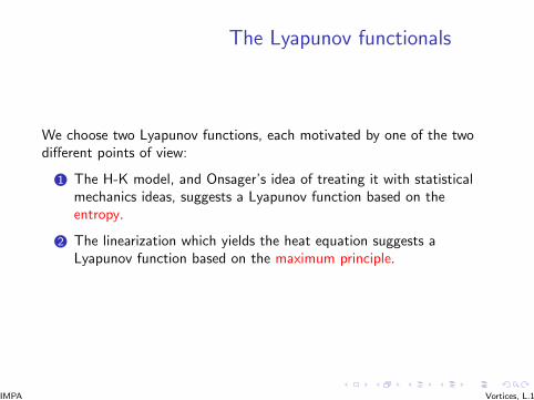
The Lyapunov functionals

We choose two Lyapunov functions, each motivated by one of the twodifferent points of view:

1 The H-K model, and Onsager’s idea of treating it with statisticalmechanics ideas, suggests a Lyapunov function based on theentropy.

2 The linearization which yields the heat equation suggests aLyapunov function based on the maximum principle.

IMPA Vortices, L.1

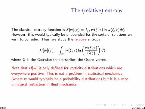
The (relative) entropy

The classical entropy function is S [w ](τ) =∫R2 w(ξ, τ) lnw(ξ, τ)dξ.

However, this would typically be unbounded for the sorts of solutions wewish to consider. Thus, we study the relative entropy

H[w ](τ) =

∫R2

w(ξ, τ) ln

(w(ξ, τ)

G (ξ)

)dξ

where G is the Gaussian that describes the Oseen vortex.

Note that H[w ] is only defined for vorticity distributions which are

everywhere positive. This is not a problem in statistical mechanics

(where w would typically be a probability distribution) but it is a very

unnatural restriction in fluid mechanics.

IMPA Vortices, L.1

The relative entropy (cont)

We need to show first that H[w ] is defined and continuous:

• Define Σ+ = {w ∈ L2(R2) | w(x) ≥ 0 almost everywhere.}. ThenH[w ] is well-defined, continuous and bounded from below onΣ+ ∩ L2(m), if m > 3.

• Also, the forward orbit of initial conditions in Σ+ ∩ L2(m) arerelatively compact (so that the ω-limit set is well defined.) Thisdepends on two facts:

• Smoothing properties of the semi-group.• Localization of the solution - one can show by estimating the

integral equation satisfied by solutions that if w0 ∈ L2(m),then w(t) consists of a piece that is in L2(m + 1) and a piecethat goes to zero in H1(m).

IMPA Vortices, L.1

The relative entropy (cont)

We need to show first that H[w ] is defined and continuous:

• Define Σ+ = {w ∈ L2(R2) | w(x) ≥ 0 almost everywhere.}. ThenH[w ] is well-defined, continuous and bounded from below onΣ+ ∩ L2(m), if m > 3.

• Also, the forward orbit of initial conditions in Σ+ ∩ L2(m) arerelatively compact (so that the ω-limit set is well defined.) Thisdepends on two facts:

• Smoothing properties of the semi-group.• Localization of the solution - one can show by estimating the

integral equation satisfied by solutions that if w0 ∈ L2(m),then w(t) consists of a piece that is in L2(m + 1) and a piecethat goes to zero in H1(m).

IMPA Vortices, L.1

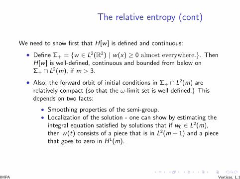
The relative entropy (cont)

We need to show first that H[w ] is defined and continuous:

• Define Σ+ = {w ∈ L2(R2) | w(x) ≥ 0 almost everywhere.}. ThenH[w ] is well-defined, continuous and bounded from below onΣ+ ∩ L2(m), if m > 3.

• Also, the forward orbit of initial conditions in Σ+ ∩ L2(m) arerelatively compact (so that the ω-limit set is well defined.) Thisdepends on two facts:

• Smoothing properties of the semi-group.• Localization of the solution - one can show by estimating the

integral equation satisfied by solutions that if w0 ∈ L2(m),then w(t) consists of a piece that is in L2(m + 1) and a piecethat goes to zero in H1(m).

IMPA Vortices, L.1

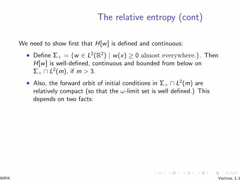
The relative entropy (cont)

We need to show first that H[w ] is defined and continuous:

• Define Σ+ = {w ∈ L2(R2) | w(x) ≥ 0 almost everywhere.}. ThenH[w ] is well-defined, continuous and bounded from below onΣ+ ∩ L2(m), if m > 3.

• Also, the forward orbit of initial conditions in Σ+ ∩ L2(m) arerelatively compact (so that the ω-limit set is well defined.) Thisdepends on two facts:

• Smoothing properties of the semi-group.

• Localization of the solution - one can show by estimating theintegral equation satisfied by solutions that if w0 ∈ L2(m),then w(t) consists of a piece that is in L2(m + 1) and a piecethat goes to zero in H1(m).

IMPA Vortices, L.1

The relative entropy (cont)

We need to show first that H[w ] is defined and continuous:

• Define Σ+ = {w ∈ L2(R2) | w(x) ≥ 0 almost everywhere.}. ThenH[w ] is well-defined, continuous and bounded from below onΣ+ ∩ L2(m), if m > 3.

• Also, the forward orbit of initial conditions in Σ+ ∩ L2(m) arerelatively compact (so that the ω-limit set is well defined.) Thisdepends on two facts:

• Smoothing properties of the semi-group.• Localization of the solution - one can show by estimating the

integral equation satisfied by solutions that if w0 ∈ L2(m),then w(t) consists of a piece that is in L2(m + 1) and a piecethat goes to zero in H1(m).

IMPA Vortices, L.1

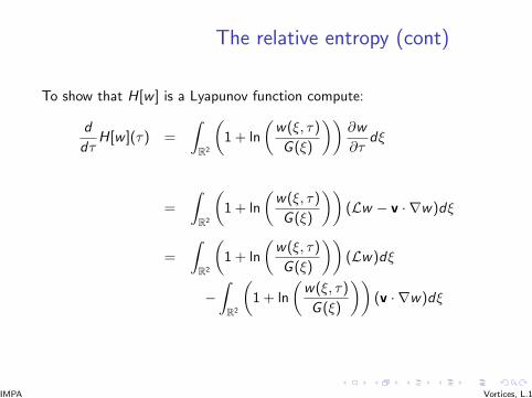
The relative entropy (cont)

To show that H[w ] is a Lyapunov function compute:

d

dτH[w ](τ) =

∫R2

(1 + ln

(w(ξ, τ)

G (ξ)

))∂w

∂τdξ

=

∫R2

(1 + ln

(w(ξ, τ)

G (ξ)

))(Lw − v · ∇w)dξ

=

∫R2

(1 + ln

(w(ξ, τ)

G (ξ)

))(Lw)dξ

−∫R2

(1 + ln

(w(ξ, τ)

G (ξ)

))(v · ∇w)dξ

IMPA Vortices, L.1

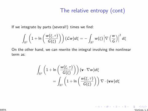
The relative entropy (cont)

If we integrate by parts (several!) times we find:∫R2

(1 + ln

(w(ξ, τ)

G (ξ)

))(Lw)dξ = −

∫R2

w(ξ)∣∣∣∇(w

G

)∣∣∣2 dξOn the other hand, we can rewrite the integral involving the nonlinearterm as:

∫R2

(1 + ln

(w(ξ, τ)

G (ξ)

))(v · ∇w)dξ

=

∫R2

(1 + ln

(w(ξ, τ)

G (ξ)

))∇ · (vw)dξ

IMPA Vortices, L.1

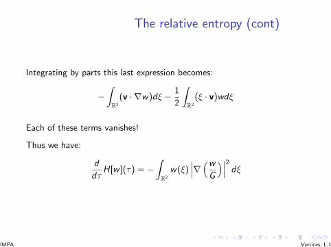
The relative entropy (cont)

Integrating by parts this last expression becomes:

−∫R2

(v · ∇w)dξ − 1

2

∫R2

(ξ · v)wdξ

Each of these terms vanishes!

Thus we have:

d

dτH[w ](τ) = −

∫R2

w(ξ)∣∣∣∇(w

G

)∣∣∣2 dξ

IMPA Vortices, L.1

The relative entropy (cont)

Integrating by parts this last expression becomes:

−∫R2

(v · ∇w)dξ − 1

2

∫R2

(ξ · v)wdξ

Each of these terms vanishes!

Thus we have:

d

dτH[w ](τ) = −

∫R2

w(ξ)∣∣∣∇(w

G

)∣∣∣2 dξ

IMPA Vortices, L.1

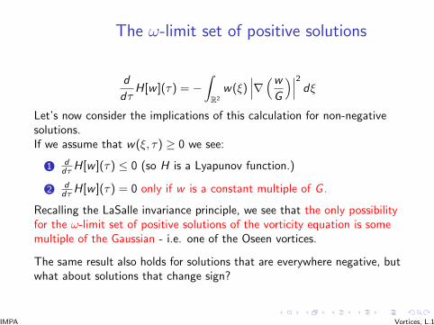
The ω-limit set of positive solutions

d

dτH[w ](τ) = −

∫R2

w(ξ)∣∣∣∇(w

G

)∣∣∣2 dξLet’s now consider the implications of this calculation for non-negativesolutions.If we assume that w(ξ, τ) ≥ 0 we see:

1 ddτH[w ](τ) ≤ 0 (so H is a Lyapunov function.)

2 ddτH[w ](τ) = 0 only if w is a constant multiple of G .

Recalling the LaSalle invariance principle, we see that the only possibilityfor the ω-limit set of positive solutions of the vorticity equation is somemultiple of the Gaussian - i.e. one of the Oseen vortices.

The same result also holds for solutions that are everywhere negative, butwhat about solutions that change sign?

IMPA Vortices, L.1

The maximum principle for the vorticityequation

One of the most powerful qualitative properties of solutions of the heatequation is the maximum principle. Closer inspection shows that just likethe heat equation, solutions of the 2D vorticity equation also satisfy amaximum principle. In particular:

• A solution that is positive for some time t0 will remain positive forany later time t > t0, and

• If the initial condition for the vorticity equation satisfies ω(z , 0) ≥ 0then the solution will be strictly positive for all times t > 0.

Note that these remarks also hold for solutions of the rescaled vorticityequation. As a consequence of these two observations, we find a second,surprisingly simple, Lyapunov functional, namely the L1(R2)-norm of thesolution!

IMPA Vortices, L.1

The L1 norm as a Lyapunov function

To show that the L1 norm is a Lyapunov function one splits a solutionthat changes sign into two pieces t

w(τ) = w1(τ)− w2(τ)

where w1,2 solve:

∂τw1 + v · ∇w1 = Lw1

∂τw2 + v · ∇w2 = Lw2

where the initial conditions for are given by

w1,0 = max(w0(ξ), 0) , w2,0 = −min(w0(ξ), 0) .

Note that both initial conditions are non-negative.

IMPA Vortices, L.1

The L1 norm as a Lyapunov function(cont)

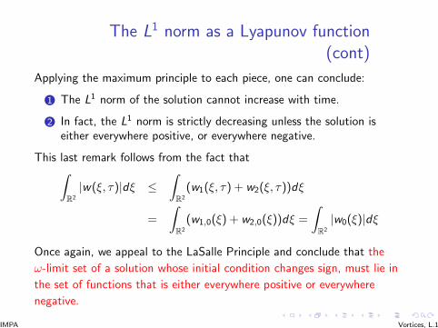
Applying the maximum principle to each piece, one can conclude:

1 The L1 norm of the solution cannot increase with time.

2 In fact, the L1 norm is strictly decreasing unless the solution iseither everywhere positive, or everywhere negative.

This last remark follows from the fact that∫R2

|w(ξ, τ)|dξ ≤∫R2

(w1(ξ, τ) + w2(ξ, τ))dξ

=

∫R2

(w1,0(ξ) + w2,0(ξ))dξ =

∫R2

|w0(ξ)|dξ

Once again, we appeal to the LaSalle Principle and conclude that the

ω-limit set of a solution whose initial condition changes sign, must lie in

the set of functions that is either everywhere positive or everywhere

negative.

IMPA Vortices, L.1

Putting the pieces together

Putting together our two Lyapunov functionals we have the followingconclusion,

1 For general solutions the ω-limit set must lie in the set of solutionsthat are everywhere positive or everywhere negative.

2 However, for such solutions, the relative entropy function impliesthat the ω-limit set must be a multiple of the Oseen vortex.

However, so far, we can only conclude that solutions for which the initialconditions are decaying relatively rapidly at infinity (i.e. solutions forwhich w0 ∈ L2(m), with m > 3) converge to an Oseen vortex.

IMPA Vortices, L.1

Extending this solution to all of L1

• We begin by proving that the forward orbit of an initial condition inL1 is relatively compact:

• Using decay estimates that go back to Carlen and Loss, one showsthat any point in the ω-limit set is actually in L2(m).

• We then apply the argument above to conclude that this point mustbe a multiple of the Oseen vortex

Thus, we conclude:

Theorem (Th. Gallay and CEW) Any solution of the two-dimensionalvorticity equation whose initial vorticity is in L1(R2) and whose totalvorticity

∫R2 ω(z , 0)dz 6= 0 will tend, as time tends to infinity, to the

Oseen vortex with parameter α =∫R2 ω(z , 0)dz .

IMPA Vortices, L.1

Extending this solution to all of L1

• We begin by proving that the forward orbit of an initial condition inL1 is relatively compact:

• Using decay estimates that go back to Carlen and Loss, one showsthat any point in the ω-limit set is actually in L2(m).

• We then apply the argument above to conclude that this point mustbe a multiple of the Oseen vortex

Thus, we conclude:

Theorem (Th. Gallay and CEW) Any solution of the two-dimensionalvorticity equation whose initial vorticity is in L1(R2) and whose totalvorticity

∫R2 ω(z , 0)dz 6= 0 will tend, as time tends to infinity, to the

Oseen vortex with parameter α =∫R2 ω(z , 0)dz .

IMPA Vortices, L.1

Extending this solution to all of L1

• We begin by proving that the forward orbit of an initial condition inL1 is relatively compact:

• Using decay estimates that go back to Carlen and Loss, one showsthat any point in the ω-limit set is actually in L2(m).

• We then apply the argument above to conclude that this point mustbe a multiple of the Oseen vortex

Thus, we conclude:

Theorem (Th. Gallay and CEW) Any solution of the two-dimensionalvorticity equation whose initial vorticity is in L1(R2) and whose totalvorticity

∫R2 ω(z , 0)dz 6= 0 will tend, as time tends to infinity, to the

Oseen vortex with parameter α =∫R2 ω(z , 0)dz .

IMPA Vortices, L.1

Extending this solution to all of L1

• We begin by proving that the forward orbit of an initial condition inL1 is relatively compact:

• Using decay estimates that go back to Carlen and Loss, one showsthat any point in the ω-limit set is actually in L2(m).

• We then apply the argument above to conclude that this point mustbe a multiple of the Oseen vortex

Thus, we conclude:

Theorem (Th. Gallay and CEW) Any solution of the two-dimensionalvorticity equation whose initial vorticity is in L1(R2) and whose totalvorticity

∫R2 ω(z , 0)dz 6= 0 will tend, as time tends to infinity, to the

Oseen vortex with parameter α =∫R2 ω(z , 0)dz .

IMPA Vortices, L.1

Extensions and Conclusions

This theorem implies that with even the slightest amount of viscositypresent, two-dimensional fluid flows will eventually approach a single,large vortex.

1 However, if the viscosity is small, this convergence may take a verylong time. (Much longer than observed in the numericalexperiments, for example.)

2 Furthermore, Onsager’s original calculations of vortex coalescencewere for an inviscid fluid model which suggests that some sort ofcoalescence should occur independent of the viscosity

Thus, while Gallay’s and my theorem says that eventually, all

two-dimensional viscous flows will approach an Oseen vortex, there

should be a variety of interesting and important behaviors that manifest

themselves in the fluid prior to reaching the asymptotic state described in

the theorem.

IMPA Vortices, L.1

Vortex Merger

One of the most important physical effects, and one of the hardest tounderstand from a mathematical point of view concerns the merger oftwo or more vortices. Clearly such mergers must take place in order forthe multitude of small vortices present in an initially turbulent flow tocoalesce into the small number of large vortices observed in numerics andexperiments.

While the Oseen vortex which characterizes the long-time asymptotics of

the flow has the property that the effects of the nonlinear terms in the

vorticity equation vanish, both numerical and experimental studies show

that the merger process is highly nonlinear and involves the filamentation

and inter-penetration of the two vortices into one another.

IMPA Vortices, L.1

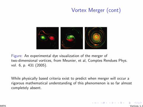
Vortex Merger (cont)

Figure: An experimental dye visualization of the merger oftwo-dimensional vortices, from Meunier, et al, Comptes Rendues Phys.vol. 6, p. 431 (2005).

While physically based criteria exist to predict when merger will occur arigorous mathematical understanding of this phenomenon is so far almostcompletely absent.

IMPA Vortices, L.1

Metastability

A second interesting phenomenon that is particularly noticeable in thenumerical simulations of two-dimensional flows on bounded domains isthe creation and persistence of metastable structures.

The origin and properties of these states in the two-dimensionalNavier-Stokes equation is still not understood but statistical mechanicalideas have again been used to propose an explanation associated with thedifferent time scales on which energy and entropy are dissipated.

IMPA Vortices, L.1

Metastability in Burgers Equation

Similar metastable phenomena also occur in the weakly viscous Burgersequation which is often used as a simplified testing ground forunderstanding the Navier-Stokes equations. Because of the simplernature of Burgers equation, one can show that the metastable statesform a one-dimensional attractive invariant manifold in the phase spaceof the equation and one can speculate that a similar dynamical systemsexplanation might account for the metastable behavior observed in thetwo-dimensional Navier-Stokes equation, as it has for the long-timeasymptotics of solutions. (Joint work with Margaret Beck at BU.)

IMPA Vortices, L.1

Summary

A distinctive feature of two-dimensional flows is the “inverse cascade” of

energy from small scales to large ones. Lars Onsager first sought to

explain this phenomenon by studying the statistical mechanics of large

collections of inviscid point vortices. While Onsager’s observation about

inviscid flows remains unexplained, dynamical systems ideas - in this case

Lyapunov functionals inspired by kinetic theory - have been used to show

that in the presence of an arbitrarily small amount of viscosity, essentially

any two-dimensional flow whose initial vorticity field is absolutely

integrable will evolve as time goes to infinity toward a single, explicitly

computable vortex.

IMPA Vortices, L.1