the topology of probability distributions on …the topology of probability distributions on...

The Topology of Probability Distributions on

ManifoldsOMER BOBROWSKI∗, and SAYAN MUKHERJEE†

Department of Mathematics,Duke University, Durham NC 27708E-mail: [email protected]

Departments of Statistical Science,Computer Science, and MathematicsInstitute for Genome Sciences & PolicyDuke University, Durham NC 27708E-mail: [email protected]

Let P be a set of n random points in Rd, generated from a probability measure on a m-dimensional manifold M ⊂ Rd. In this paper we study the homology of U(P, r) – the union ofd-dimensional balls of radius r around P, as n→∞, and r → 0. In addition we study the criticalpoints of dP – the distance function from the set P. These two objects are known to be related viaMorse theory. We present limit theorems for the Betti numbers of U(P, r), as well as for numberof critical points of index k for dP . Depending on how fast r decays to zero as n grows, thesetwo objects exhibit different types of limiting behavior. In one particular case (nrm ≥ C logn),we show that the Betti numbers of U(P, r) perfectly recover the Betti numbers of the originalmanifold M, a result which is of significant interest in topological manifold learning.

AMS 2000 subject classifications: Primary 60D05, 60F15, 60G55; secondary 55U10.Keywords: Random complexes, Point process, Random Betti numbers, Stochastic topology.

1. Introduction

The incorporation of geometric and topological concepts for statistical inference is at theheart of spatial point process models, manifold learning, and topological data analysis.The motivating principle behind manifold learning is using low dimensional geometricsummaries of the data for statistical inference [4, 10, 21, 31, 50]. In topological data anal-ysis, topological summaries of data are used to infer or extract underlying structure inthe data [19, 22, 40, 49, 52]. In the analysis of spatial point processes, limiting distribu-tions of integral-geometric quantities such as area and boundary length [24, 42, 48, 36],Euler characteristic of patterns of discs centered at random points [36, 51], and the Palm

∗OB was supported by DARPA: N66001-11-1-4002Sub#8†SM is pleased to acknowledge the support of NIH (Systems Biology): 5P50-GM081883, AFOSR:

FA9550-10-1-0436, NSF CCF-1049290, and NSF DMS-1209155.

1

arX

iv:1

307.

1123

v2 [

mat

h.PR

] 1

Mar

201

4

mailto:[email protected]

mailto:[email protected]

2 Bobrowski and Mukherjee

mean (the mean number of pairs of points within a radius r) [24, 42, 51, 48] have beenused to characterize parameters of point processes, see [36] for a short review.

A basic research topic in both manifold learning and topological data analysis isunderstanding the distribution of geometric and topological quantities generated by astochastic process. In this paper we consider the standard model in topological dataanalysis and manifold learning – the stochastic process is a random sample of pointsP drawn from a distribution supported on a compact m-dimensional manifold M, em-bedded in Rd. In both geometric and topological data analysis, understanding the localneighborhood structure of the data is important. Thus, a central parameter in any anal-ysis is the size r (radius) of a local neighborhood and how this radius scales with thenumber of observations.

We study two different, yet related, objects. The first object is the union of the r-ballsaround the random sample, denoted by U(P, r). For this object, we wish to study itshomology, and in particular its Betti numbers. Briefly, the Betti numbers are topologicalinvariants measuring the number of components and holes of different dimensions. Equiv-alently, all the results in this paper can be phrased in terms of the Cech complex C(P, r).A simplicial complex is a collection of vertices, edges, triangles, and higher dimensionalfaces, and can be thought of as a generalization of a graph. The Cech complex C(P, r) issimplicial complex where each k-dimensional face corresponds to an intersection of k+ 1balls in U(P, r) (see Definition 2.4). By the famous ‘Nerve Lemma’ (cf. [15]), U(P, r)has the same homology as C(P, r). The second object of study is the distance functionfrom the set P, denoted by dP , and its critical points. The connection between thesetwo objects is given by Morse theory, which will be reviewed later. In a nutshell, Morsetheory describes how critical points of a given function either create or destroy homologyelements (connected components and holes) of sublevel sets of that function.

We characterize the limit distribution of the number of critical points of dP , as wellas the Betti numbers of U(P, r). Similarly to many phenomena in random geometricgraphs as well as random geometric complexes in Euclidean spaces [29, 30, 33, 46], thequalitative behavior of these distributions falls into three main categories based on howthe radius r scales with the number of samples n. This behavior is determined by theterm nrm, where m is the intrinsic dimension of the manifold. This term can be thoughtof as the expected number of points in a ball of radius r. We call the different categories– the sub-critical (nrm → 0), critical (nrm → λ) and super-critical (nrm →∞) regimes.The union U(P, r) exhibits very different limiting behavior in each of these three regimes.In the sub-critical regime, U(P, r) is very sparse and consists of many small particles,with very few holes. In the critical regime, U(P, r) has O(n) components as well as holesof any dimension k < m. From the manifold learning perspective, the most interestingregime would be the super-critical. One of the main result in this paper (see Theorem4.9) states that if we properly choose the radius r within the super-critical regime, thehomology of the random space U(P, r) perfectly recovers the homology of the originalmanifold M. This result extends the work in [44] for a large family of distributions onM, requires much weaker assumptions on the geometry of the manifold, and is provedto happen almost surely.

The study of critical points for the distance function provides additional insights on

The Topology of Probability Distributions on Manifolds 3

the behavior of U(P, r) via Morse theory, we return to this later in the paper. WhileBetti numbers deal with ‘holes’ which are typically determined by global phenomena, thestructure of critical points is mostly local in nature. Thus, we are able to derive preciseresults for critical points even in cases where we do not have precise analysis of Bettinumbers. One of the most interesting consequence of the critical point analysis in thispaper relates to the Euler characteristic of U(P, r). One way to think about the Eulercharacteristic of a topological spaces S is as integer “summary” of the Betti numbersgiven by χ(S) =

∑k(−1)kβk(S). Morse theory enables us to compute χ(U(P, r)) using

the critical points of the distance function dP (see Section 4.2). This computation mayprovide important insights on the behavior of the Betti numbers in the critical regime.We note that the equivalent result for Euclidean spaces appeared in [13].

In topological data analysis there has been work on understanding properties of ran-dom abstract simplicial complexes generated from stochastic processes [1, 2, 5, 13, 28, 29,30, 32, 46, 47] and non-asymptotic bounds on the convergence or consistency of topolog-ical summaries as the number of points increase [11, 17, 18, 20, 23, 44, 45]. The centralidea in these papers has been to study statistical properties of topological summaries ofpoint cloud data. There has also been an effort to characterize the topology of a distri-bution (for example a noise model) [1, 2, 30]. Specifically, the results in our paper adaptthe results in [13, 29, 30] from the setting of a distribution in Euclidean space to onesupported on a manifold.

There is a natural connection of the results in this paper with results in point processes,specifically random set models such as the Poisson-Boolean model [37]. The stochasticprocess we study in this paper is an example of a random set model – stochastic modelsthat place probability distributions on regions or geometric objects [34, 41]. Classically,people have studied limiting distributions of quantities such as volume, surface area, in-tegral of mean curvature and Euler characteristic generated from the random set model.Initial studies examined second order statistics, summaries of observations that measureposition or interaction among points, such as the distribution function of nearest neigh-bors, the spherical contact distribution function, and a variety of other summaries such asRipley’s K-function, the L-function and the pair correlation function, see [24, 42, 48, 51].It is known that there are limitations in only using second order statistics since onecan state different point processes that have the same second order statistics [8]. In thespatial statistics literature our work is related to the use of morphological functions forpoint processes where a ball of radius r is placed around each point sampled from thepoint process and the topology or morphology of the union of these balls is studied.Our results are also related to ideas in the statistics and statistical physics of randomfields, see [3, 7, 14, 53, 54], a random process on a manifold can be thought of as anapproximation of excursion sets of Gaussian random fields or energy landscapes.

The paper is structured as follows. In Section 2 we give a brief introduction to thetopological objects we study in this paper. In Section 3 we state the probability modeland define the relevant topological and geometric quantities of study. In sections 4 and5 we state our main results and proofs, respectively.


2. Topological Ingredients

In this paper we study two topological objects generated from a finite random pointcloud P ⊂ Rd (a set of points in Rd).

1. Given the set P we defineU(P, ε) :=

⋃p∈P

Bε(p), (2.1)

where Bε(p) is a d-dimensional ball of radius ε centered at p. Our interest in thispaper is in characterizing the homology – in particular the Betti numbers of thisspace, i.e. the number of components, holes, and other types of voids in the space.

2. We define the distance function from P as

dP(x) := minp∈P‖x− p‖ , x ∈ Rd. (2.2)

As a real valued function, dP : Rd → R might have critical points of different types(i.e. minimum, maximum and saddle points). We would like to study the amountand type of these points.

In this section we give a brief introduction to the topological concepts behind thesetwo objects. Observe that the sublevel sets of the distance function are

d−1P ((−∞, r]) :={x ∈ Rd : dP(x) ≤ r

}= U(P, r).

Morse theory, discussed later in this section, describes the interplay between criticalpoints of a function and the homology of its sublevel sets, and hence provides the linkbetween our two objects of study.

2.1. Homology and Betti Numbers

Let X be a topological space. The k-th Betti number of X, denoted by βk(X) is the rankof Hk(X) – the k-th homology group of X. This definition assumes that the reader has abasic grounding in algebraic topology. Otherwise, the reader should be willing to accepta definition of βk(X) as the number of k-dimensional ‘cycles’ or ‘holes’ in X, where ak-dimensional hole can be thought of as anything that can be continuously transformedinto the boundary of a (k + 1)-dimensional shape. The zeroth Betti number, β0(X), ismerely the number of connected components in X. For example, the 2-dimensional torusT 2 has a single connected component, two non-trivial 1-cycles, and a 2-dimensional void.Thus, we have that β0(T 2) = 1, β1(T 2) = 2, and β2(T 2) = 1. Formal definitions ofhomology groups and Betti numbers can be found in [27, 43].

2.2. Critical Points of the Distance Function

The classical definition of critical points using calculus is as follows. Let f : Rd → R bea C2 function. A point c ∈ R is called a critical point of f if ∇f(c) = 0, and the real


number f(c) is called a critical value of f . A critical point c is called non-degenerate if theHessian matrix Hf (c) is non-singular. In that case, the Morse index of f at c, denoted byµ(c) is the number of negative eigenvalues of Hf (c). A C2 function f is a Morse functionif all its critical points are non-degenerate, and its critical levels are distinct.

Note, the distance function dP is not everywhere differentiable, therefore the defi-nition above does not apply. However, following [26], one can still define a notion ofnon-degenerate critical points for the distance function, as well as their Morse index. Ex-tending Morse theory to functions that are non-smooth has been developed for a varietyof applications [9, 16, 26, 35]. The class of functions studied in these papers have beenthe minima (or maxima) of a functional and called ‘min-type’ functions. In this section,we specialize those results to the case of the distance function.

We start with the local (and global) minima of dP , the points of P where dP = 0, andcall these critical points with index 0. For higher indices, we have the following definition.

Definition 2.1. A point c ∈ Rd is a critical point of index k of dP , where 1 ≤ k ≤ d,if there exists a subset Y of k + 1 points in P such that:

1. ∀y ∈ Y : dP(c) = ‖c− y‖, and, ∀p ∈ P\Y we have ‖c− p‖ > dP(p).2. The points in Y are in general position (i.e. the k + 1 points of Y do not lie in a

(k − 1)-dimensional affine space).3. c ∈ conv◦(Y), where conv◦(Y) is the interior of the convex hull of Y (an open

k-simplex in this case).

The first condition implies that dP ≡ dY in a small neighborhood of c. The secondcondition implies that the points in Y lie on a unique (k − 1)- dimensional sphere. Weshall use the following notation:

S(Y) = The unique (k − 1)-dimensional sphere containing Y, (2.3)

C(Y) = The center of S(Y) in Rd, (2.4)

R(Y) = The radius of S(Y), (2.5)

B(Y) = The open ball in Rd with radius R(Y) centered at C(Y). (2.6)

Note that S(Y) is a (k − 1)-dimensional sphere, whereas B(Y) is a d-dimensional ball.Obviously, S(Y) ⊂ B(Y), but unless k = d, S is not the boundary of B. Since the criticalpoint c in Definition 2.1 is equidistant from all the points in Y, we have that c = C(Y).Thus, we say that c is the unique index k critical point generated by the k + 1 points inY. The last statement can be rephrased as follows:

Lemma 2.2. A subset Y ⊂ P of k + 1 points in general position generates an index kcritical point if, and only if, the following two conditions hold:

CP1 C(Y) ∈ conv◦(Y),CP2 P ∩B(Y) = ∅.

Furthermore, the critical point is C(Y) and the critical value is R(Y).


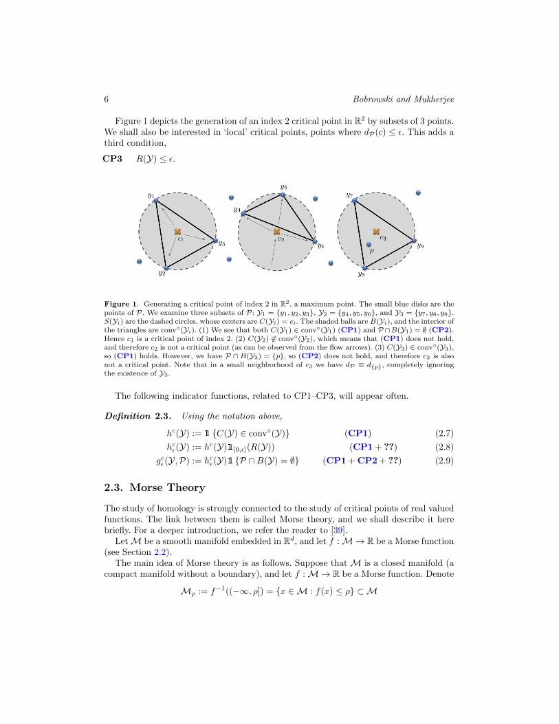
Figure 1 depicts the generation of an index 2 critical point in R2 by subsets of 3 points.We shall also be interested in ‘local’ critical points, points where dP(c) ≤ ε. This adds athird condition,

CP3 R(Y) ≤ ε.

Figure 1. Generating a critical point of index 2 in R2, a maximum point. The small blue disks are thepoints of P. We examine three subsets of P: Y1 = {y1, y2, y3}, Y2 = {y4, y5, y6}, and Y3 = {y7, y8, y9}.S(Yi) are the dashed circles, whose centers are C(Yi) = ci. The shaded balls are B(Yi), and the interior ofthe triangles are conv◦(Yi). (1) We see that both C(Y1) ∈ conv◦(Y1) (CP1) and P ∩B(Y1) = ∅ (CP2).Hence c1 is a critical point of index 2. (2) C(Y2) 6∈ conv◦(Y2), which means that (CP1) does not hold,and therefore c2 is not a critical point (as can be observed from the flow arrows). (3) C(Y3) ∈ conv◦(Y3),so (CP1) holds. However, we have P ∩ B(Y3) = {p}, so (CP2) does not hold, and therefore c3 is alsonot a critical point. Note that in a small neighborhood of c3 we have dP ≡ d{p}, completely ignoringthe existence of Y3.

The following indicator functions, related to CP1–CP3, will appear often.

Definition 2.3. Using the notation above,

hc(Y) := 1 {C(Y) ∈ conv◦(Y)} (CP1) (2.7)

hcε(Y) := hc(Y)1[0,ε](R(Y)) (CP1 + ??) (2.8)

gcε(Y,P) := hcε(Y)1 {P ∩B(Y) = ∅} (CP1 + CP2 + ??) (2.9)

2.3. Morse Theory

The study of homology is strongly connected to the study of critical points of real valuedfunctions. The link between them is called Morse theory, and we shall describe it herebriefly. For a deeper introduction, we refer the reader to [39].

LetM be a smooth manifold embedded in Rd, and let f :M→ R be a Morse function(see Section 2.2).

The main idea of Morse theory is as follows. Suppose that M is a closed manifold (acompact manifold without a boundary), and let f :M→ R be a Morse function. Denote

Mρ := f−1((−∞, ρ]) = {x ∈M : f(x) ≤ ρ} ⊂ M


(sublevel sets of f). If there are no critical levels in (a, b], thenMa andMb are homotopyequivalent, and in particular have the same homology. Next, suppose that c is a criticalpoint of f with Morse index k, and let v = f(c) be the critical value at c. Then thehomology of Mρ changes at v in the following way. For a small enough ε we have thatthe homology of Mv+ε is obtained from the homology of Mv−ε by either adding agenerator to Hk (increasing βk by one) or terminating a generator of Hk−1 (decreasingβk−1 by one). In other words, as we pass a critical level, either a new k-dimensional holeis formed, or an existing (k − 1)-dimensional hole is terminated (filled up).

Note, that while classical Morse theory deals with Morse functions (and in particular,C2) on compact manifolds, its extension for min-type functions presented in [26] enablesus to apply these concepts to the distance function dP as well.

2.4. Cech Complexes and the Nerve Lemma

The Cech complex generated by a set of points P is a simplicial complex, made up ofvertices, edges, triangles and higher dimensional faces. While its general definition isquite broad, and uses intersections of arbitrary nice sets, the following special case usingintersection of Euclidean balls will be sufficient for our analysis.

Definition 2.4 (Cech complex). Let P = {x1, x2, . . .} be a collection of points in Rd,and let ε > 0. The Cech complex C(P, ε) is constructed as follows:

1. The 0-simplices (vertices) are the points in P.2. An n-simplex [xi0 , . . . , xin ] is in C(P, ε) if

⋂nk=0Bε(xik) 6= ∅.

Figure 2 depicts a simple example of a Cech complex in R2. An important result,

Figure 2. The Cech complex C(P, ε), for P = {x1, . . . , x6} ⊂ R2, and some ε. The complex contains 6vertices, 7 edges, and a single 2-dimensional face.

known as the ‘Nerve Lemma’, links the Cech complex C(P, ε) and the neighborhood setU(P, ε), and states that they are homotopy equivalent, and in particular they have thesame homology groups (cf. [15]). Thus, for example, they have the same Betti numbers.


Our interest in the Cech complex is twofold. Firstly, the Cech complex is a high-dimensional analogue of a geometric graph. The study of random geometric graphs iswell established (cf. [46]). However, the study of higher dimensional geometric complexesis at its early stages. Secondly, many of the proofs in this paper are combinatorial innature. Hence, it is usually easier to examine the Cech complex C(P, ε), rather than thegeometric structure U(P, ε).

3. Model Specification and Relevant Definitions

In this section we specify the stochastic process on a manifold that generates the pointsample and topological summaries we will characterize.

The point processes we examine in this paper live in Rd and are supported on a m-dimensional manifold M ⊂ Rd (m < d). Throughout this paper we assume that M isclosed (i.e. compact and without a boundary) and smooth.

Let M be such a manifold, and let f : M→ R be a probability density function onM, which we assume to be bounded and measurable. If X is a random variable in Rdwith density f , then for every A ⊂ Rd

F (A) := P (X ∈ A) =

∫A∩M

f(x) dx,

where dx is the volume form on M.We consider two models for generating point clouds on the manifold M:

(1) Random sample: n points are drawn Xn = {X1, X2, . . . , Xn}iid∼ f ,

(2) Poisson process: the points are drawn from a spatial Poisson process with intensityfunction λn := nf . The spatial Poisson process has the following two properties:

(a) For every region A ⊂ M, the number of points in the region NA := |Pn ∩A|is distributed as a Poisson random variable

NA ∼ Poisson (nF (A)) ;

(b) For every A,B ⊂M such that A ∩B = ∅, the random variables NA and NBare independent.

These two models behave very similarly. The main difference is that the number ofpoints in Xn is exactly n, while the number of points in Pn is distributed Poisson (n).Since the Poisson process has computational advantages, we will present all the resultsand proofs in this paper in terms of Pn. However, the reader should keep in mind thatthe results also apply to samples generated by the first model (Xn), with some minoradjustments. For a full analysis of the critical points in the Euclidean case for bothmodels, see [12].


The stochastic objects we study in this paper are the union U(Pn, ε) (defined in (2.1)),and the distance function dPn (defined in (2.2)). The random variables we examine arethe following. Let rn be a sequence of positive numbers, and define

βk,n := βk(U(Pn, rn)), (3.1)

to be the k-th Betti number of U(Pn, rn), for 0 ≤ k ≤ d− 1. The values βk,n form a setof well defined integer random variables.

For 0 ≤ k ≤ d, denote by Ck,n the set of critical points with index k of the distancefunction dPn . Let rn be positive , and define the set of ‘local’ critical points as

CLk,n := {c ∈ Ck,n : dPn(c) < rn} = Ck,n ∩ U(Pn, rn); (3.2)

and its size asNk,n :=

∣∣CLk,n∣∣ . (3.3)

The values Nk,n also form a set of integer valued random variables. From the discussion in

Section 2.3 we know that there is a strong connection between the set of values {βk,n}d−1k=0

and {Nk,n}dk=0. We are interested in studying the limiting behavior of these two sets ofrandom variables, as n→∞, and rn → 0.

4. Results

In this section we present limit theorems for the random variables βk,n and Nk,n, asn→∞, and rn → 0. Similarly to the results presented in [13, 29], the limiting behaviorsplits into three main regimes. In [13, 29] the term controlling the behavior is nrdn, whered is the ambient dimension. This value can be thought of as representing the expectednumber of points occupying a ball of radius rn. Generating samples from a m-dimensionalmanifold (rather than the entire d-dimensional space) changes the controlling term to benrmn . This new term can be thought of as the expected number of points occupying ageodesic ball of radius rn on the manifold. We name the different regimes the sub-critical(nrmn → 0), the critical (nrmn → λ), and the super-critical (nrmn → ∞). In this sectionwe will present limit theorems for each of these regimes separately. First, however, wepresent a few statements common to all regimes.

The index 0 critical points (minima) of dPn are merely the points in Pn. Therefore,N0,n = |Pn| ∼ Poisson (n), so our focus is on the higher indexes critical points.

Next, note that if the radius rn is small enough, one can show that U(Pn, rn) canbe continuously transformed into a subset M′ of M (by a ‘deformation retract’), andthis implies that U(Pn, rn) has the same homology as M′. Since M is m-dimensional,βk(M) = 0 for every k > m, and the same goes for every subset ofM. In addition, exceptfor the coverage regime (see Section 4.3),M′ is a union of strict subsets of the connectedcomponents ofM, and thus must have βm(M′) = 0 as well. Therefore, we have that βk,n= 0 for every k ≥ m. By Morse theory, this also implies that Nk,n = 0 for every k > m.The results we present in the following sections therefore focus on β0,n, . . . , βm−1,n andN1,n, . . . , Nm,n only.


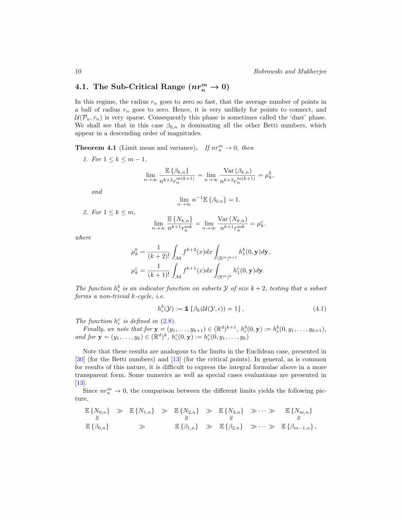
4.1. The Sub-Critical Range (nrmn → 0)

In this regime, the radius rn goes to zero so fast, that the average number of points ina ball of radius rn goes to zero. Hence, it is very unlikely for points to connect, andU(Pn, rn) is very sparse. Consequently this phase is sometimes called the ‘dust’ phase.We shall see that in this case β0,n is dominating all the other Betti numbers, whichappear in a descending order of magnitudes.

Theorem 4.1 (Limit mean and variance). If nrmn → 0, then

1. For 1 ≤ k ≤ m− 1,

limn→∞

E {βk,n}nk+2r

m(k+1)n

= limn→∞

Var (βk,n)

nk+2rm(k+1)n

= µbk,

andlimn→∞

n−1E {β0,n} = 1.

2. For 1 ≤ k ≤ m,

limn→∞

E {Nk,n}nk+1rmkn

= limn→∞

Var (Nk,n)

nk+1rmkn= µck.

where

µbk =1

(k + 2)!

∫Mfk+2(x)dx

∫(Rm)k+1

hb1(0,y)dy,

µck =1

(k + 1)!

∫Mfk+1(x)dx

∫(Rm)k

hc1(0,y)dy.

The function hbε is an indicator function on subsets Y of size k+ 2, testing that a subsetforms a non-trivial k-cycle, i.e.

hbε(Y) := 1 {βk(U(Y, ε)) = 1} , (4.1)

The function hcε is defined in (2.8).Finally, we note that for y = (y1, . . . , yk+1) ∈ (Rd)k+1, hbε(0,y) := hbε(0, y1, . . . , yk+1),

and for y = (y1, . . . , yk) ∈ (Rd)k, hcε(0,y) := hcε(0, y1, . . . , yk)

Note that these results are analogous to the limits in the Euclidean case, presented in[30] (for the Betti numbers) and [13] (for the critical points). In general, as is commonfor results of this nature, it is difficult to express the integral formulae above in a moretransparent form. Some numerics as well as special cases evaluations are presented in[13].

Since nrmn → 0, the comparison between the different limits yields the following pic-ture,

E {N0,n} � E {N1,n} � E {N2,n} � E {N3,n} � · · · � E {Nm,n}

≈ ≈ ≈ ≈

E {β0,n} � E {β1,n} � E {β2,n} � · · · � E {βm−1,n} ,


where by an ≈ bn we mean that an/bn → c ∈ (0,∞) and by an � bn we mean thatan/bn → ∞. This diagram implies that in the sub-critical phase the dominating Bettinumber is β0. It is significantly less likely to observe any cycle, and it becomes less likelyas the cycle dimension increases. In other words, U(Pn, rn) consists mostly of smalldisconnected particles, with relatively few holes.

Note that the limit of the term nk+1rmkn can be either zero, infinity, or anything inbetween. For each of these cases, the limiting distribution of either βk−1,n or Nk,n iscompletely different. The results for the number of critical points are as follows.

Theorem 4.2 (Limit distribution). Let nrmn → 0, and 1 ≤ k ≤ m,

1. If limn→∞ nk+1rkn = 0, then

Nk,nL2

−−→ 0.

If, in addition,∑∞n=1 n

k+1rmkn <∞, then

Nk,na.s.−−→ 0.

2. If limn→∞ nk+1rmkn = α ∈ (0,∞), then

Nk,nL−→ Poisson (αµck) .

3. If limn→∞ nk+1rmkn =∞, then

Nk,n − E {Nk,n}(nk+1rmkn )1/2

L−→ N (0, µck).

For βk,n the theorem above needs two adjustments. Firstly, we need to replace the

term nk+1rmkn with nk+2rm(k+1)n , and µck with µbk (similarly to Theorem 4.1). Secondly,

the proof of the central limit theorem in part 3 is more delicate, and requires an additionalassumption that nrmn ≤ n−ε for some ε > 0.

4.2. The Critical Range (nrmn → λ ∈ (0,∞))

In the dust phase, β0,n was O(n), while the other Betti numbers of U(Pn, rn) were ofa much lower magnitude. In the critical regime, this behavior changes significantly, andwe observe that all the Betti numbers (as well as counts of all critical points) are O(n).In other words, the behavior of U(Pn, rn) is much more complex, in the sense that itconsists of many cycles of any dimension 1 ≤ k ≤ m− 1.

Unfortunately, in the critical regime, the combinatorics of cycle counting becomeshighly complicated. However, we can still prove the following qualitative result, whichshows that E {βk,n} = O(n).

Theorem 4.3. If nrmn → λ ∈ (0,∞), then for 1 ≤ k ≤ m− 1,

0 < lim infn→∞

n−1E {βk,n} ≤ lim supn→∞

n−1E {βk,n} <∞.


Fortunately, the situation with the critical points is much better. A critical point ofindex k is always generated by subsets Y of exactly k + 1 points. Therefore, nothingessentially changes in our methods when we turn to examine the limits of Nk,n. We canprove the following limit theorems.

Theorem 4.4. If nrmn → λ ∈ (0,∞), then for 1 ≤ k ≤ m,

limn→∞

E {Nk,n}n

= γk(λ),

limn→∞

Var (Nk,n)

n= σ2

k(λ),

Nk,n − E {Nk,n}√n

L−→ N (0, σ2k(λ)).

where

γk(λ) :=λk

(k + 1)!

∫M

∫(Rm)k

fk+1(x)hc1(0,y)e−λωmRm(0,y)f(x)dydx,

R, hcε, are defined in (2.5), (2.8), respectively. The expression defining σ2k(λ) is rather

complicated, and will be discussed in the proof.

The term ωm stands for the volume of the unit ball in Rm. As mentioned above, ingeneral it is difficult to present a more explicit formula for γk(λ). However, for m ≤ 3 andf ≡ 1 (the uniform distribution) it is possible to evaluate γk(λ) (using tedious calculusarguments which we omit here). For m = 3 these computations yield -

γ1(λ) = 4(1− e− 43πλ),

γ2(λ) = (1 +π2

16)(3− 3e−

43πλ − 4πλe−

43πλ),

γ3(λ) =π2

48(9− 9e−

43πλ − 12πλe−

43πλ − 8π2λ2e−

43πλ),

and

d

dλγ1(λ) =

16

3πe−

43πλ,

d

dλγ2(λ) = (16 + π2)

π2

3λe−

43πλ,

d

dλγ3(λ) =

2

9π5λ2e−

43πλ,

where ddλγk(λ) can be thought of as the rate at which critical points appear. Figures 3(a)

and 3(b) are the graphs of these curves.As mentioned earlier, in this regime we cannot get exact limits for the Betti numbers.

However, we can use the limits of the critical points to compute the limit of another


Figure 3. The graphs of the γk functions for the case where m = 3, and f ≡ 1. (a) The graphs forthe limiting number of critical points γk(λ). (b) The graphs for the rate of appearance of critical pointsgiven by d

dλγk(λ). (c) The limiting (normalized) Euler characteristic given by 1− γ1(λ) + γ2(λ)− γ3(λ).

important topological invariant of U(Pn, rn) – its Euler characteristic. The Euler char-acteristic χn of U(Pn, rn) (or, equivalently, of C(Pn, rn)) has a number of equivalentdefinitions. One of the definitions, via Betti numbers, is

χn =

m∑k=0

(−1)kβk,n. (4.2)

In other words, the Euler characteristic “summarizes” the information contained in Bettinumbers to a single integer. Using Morse theory, we can also compute χn from the criticalpoints of the distance function by

χn =

m∑k=0

(−1)kNk,n.

Thus, using Theorem 4.4 we have the following result.

Corollary 4.5. If nrmn → λ ∈ (0,∞), then

limn→∞

n−1E {χn} = 1 +

m∑k=1

(−1)kγk(λ).

This limit provides us with partial, yet important, topological information about thecomplex U(Pn, rn) in the critical regime. While we are not able to derive the preciselimits for each of the Betti numbers individually, we can provide the asymptotic resultfor their “summary”. In addition, numerical experiments (cf. [30]) seem to suggest thatat different ranges of radii there is at most a single degree of homology which dominatesthe others. This implies that χn ≈ (−1)kβk,n for the appropriate range. If this heuristiccould be proved in the future, the result above could be used to approximate βk,n in


the critical regime. In Figure 3(c) we present the curve of the limit Euler characteristic(normalized) for m = 3 and f ≡ 1. Finally, we note that while we presented the limitfor the first moment of the Euler characteristic, using Theorem 4.4 one should be ableto prove stronger limit results as well.

4.3. The Super-Critical Range (nrmn → ∞)

Once we move from the critical range into the super-critical, the complex U(Pn, rn)becomes more and more connected, and less porous. The “noisy” behavior (in the sensethat there are many holes of any possible dimension) we observed in the critical regimevanishes. This, however does not happen immediately. The scale at which major changesoccur is when nrmn ∝ log n.

The main difference between this regime and the previous two, is that while the numberof critical points is still O(n), the Betti numbers are of a much lower magnitude. In fact,for rn big enough, we observe that βk,n ∼ βk(M), which implies that these values areO(1).

For the super-critical phase we have to assume that fmin := infx∈M f(x) > 0. Thiscondition is required for the proofs, but is not a technical issue only. Having a pointx ∈M where f(x) = 0 implies that in the vicinity of x we expect to have relatively fewpoints in Pn. Since the radius of the balls generating U(Pn, rn) goes to zero, this areamight become highly porous or disconnected , and look more similar to other regimes.However, we postpone this study for future work.

We start by describing the limit behavior of the critical points, which is very similarto that of the critical regime.

Theorem 4.6. If rn → 0, and nrmn →∞, then for 1 ≤ k ≤ m,

limn→∞

E {Nk,n}n

= γk(∞),

limn→∞

Var (Nk,n)

n= σ2

k(∞),

Nk,n − E {Nk,n}√n

L−→ N (0, σ2k(∞)).

where

γk(∞) = limλ→∞

γk(λ) =1

(k + 1)!

∫(Rm)k

hc(0,y)e−ωmRm(0,y) dy,

R, hc, are defined in (2.5), (2.7), respectively.

ωm is the volume of the unit ball in Rm The combinatorial analysis of the Bettinumbers βk,n in the super-critical regime suffers from the same difficulties described inthe critical regime. However, in the special case that rn is big enough so that U(Pn, rn)covers M, we can use a different set of methods to derive limit results for βk,n.


The Coverage Regime

In [46](Section 13.2), it is shown that for samples generated on a m-dimensional torus,the complex U(Pn, rn) becomes connected when nrmn ≈ (ωmfmin2m)−1 log n. This resultcould be easily extended to the general class of manifolds studied in this paper (althoughwe will not pursue that here). While the complex is reaching a finite number of compo-nents (β0,n → β0(M)), it is still possible for it to have very large Betti numbers for k ≥ 1.In this paper we are interested in a threshold for which we have βk,n = βk(M) for all k(and not just β0). We will show that this threshold is when nrmn = (ωmfmin)−1 log n, sothat rn is twice than the radius required for connectivity.

To prove this result we need two ingredients. The first one is a coverage statement,presented in the following proposition.

Proposition 4.7 (Coverage). If nrmn ≥ C log n, then:

1. If C > (ωmfmin)−1, then

limn→∞

P (M⊂ U(Pn, rn)) = 1.

2. If C > 2(ωmfmin)−1, then almost surely there exists M > 0 (possibly random), suchthat for every n > M we have M⊂ U(Pn, rn).

The second ingredient is a statement about the critical points of the distance function,unique to the coverage regime. Let rn be any sequence of positive numbers such that (a)

rn → 0, and (b) rn > rn for every n. Define Nk,n to be the number of critical points of

dPn with critical value bounded by rn. Obviously, Nk,n ≥ Nk,n, but we will prove thatchoosing rn properly, these two quantities are asymptotically equal.

Proposition 4.8. If nrmn ≥ C log n, then:


limn→∞

P(Nk,n = Nk,n, ∀1 ≤ k ≤ m

)= 1.

2. If C > 2(ωmfmin)−1, then almost surely there exists M > 0 (possibly random), suchthat for n > M

Nk,n = Nk,n, ∀1 ≤ k ≤ m.

In other words, if rn is chosen properly, then U(Pn, rn) contains all the ‘local’ (smallvalued) critical points of dPn .

Combining the fact that M is covered, the deformation retract argument in [44], andthe fact that there are no local critical points outside U(Pn, rn), using Morse theory, wehave the desired statement about the Betti numbers.

Theorem 4.9 (Convergence of the Betti Numbers). If rn → 0, and nrmn ≥ C log n,then:



limn→∞

P (βk,n = βk(M), ∀0 ≤ k ≤ m) = 1.

2. If C > 2(ωmfmin)−1, then almost surely there exists M > 0, such that for n > M

βk,n = βk(M), ∀0 ≤ k ≤ m.

Note that M (the exact point of convergence) is random.

A common problem in topological manifold learning is the following:Given a set of random points P, sampled from an unknown manifold M, how can oneinfer the topological features of M?The last theorem provides a possible solution. Draw balls around P, with a radius rsatisfying the condition in Theorem 4.9. As the sample size grows it is guaranteed thatthe Betti numbers computed from the union of the balls will recover those of the originalmanifold M. This solution is in the spirit of the result in [44], where a bound on therecovery probability is given as a function of the sample size and the condition numberof the manifold, for a uniform measure onM. The result in 4.9 applies for a larger classof probability measures onM, require much weaker assumptions on the geometry of themanifold (the result in [44] requires the knowledge of the condition number, or the reach,of the manifold), and convergence is shown to occur almost surely.

5. Proofs

In this section we provide proofs for the statements in this paper. We note that the proofsof theorems 4.1 - 4.6 are similar to the proofs of the equivalent statements in [29, 30] (forthe Betti numbers), and in [13] (for the critical points). There are, however, significantdifferences when dealing with samples on a closed manifold. We provide detailed proofsfor the limits of the first moments, demonstrating these differences, and refer the readerto [13, 29, 30] for the rest of the details.

5.1. Some Notation and Elementary Considerations

This section is devoted to prove the results in Section 4, and is organized according tosituations: sub-critical (dust), critical, and super-critical. In this section we list somecommon notation and note some simple facts that will be used in the proofs.

• Henceforth, k will be fixed, and whenever we use Y,Y ′ or Yi we implicitly assume(unless stated otherwise) that either |Y| = |Y ′| = |Yi| = k + 2 for k-cycles, or |Y| =|Y ′| = |Yi| = k + 1 for index k critical points.

• Usually, finite subsets of Rd will be denoted calligraphically (X ,Y). However insideintegrals we use boldfacing and lower case (x,y).


• For every x ∈ M we denote by TxM the tangent space of M at x, and define expx :TxM→M to be the exponential map at x. Briefly, this means that for every v ∈ TxM,the point expx(v) is the point on the unique geodesic leaving x in the direction of v,after traveling a geodesic distance equal to ‖v‖.

• For x ∈ Rd, x ∈Mk+1 and y ∈ (Rm)k, we use the shorthand

f(x) := f(x1)f(x2) · · · f(xk+1),

f(x, expx(v)) := f(x)f(expx(v1)) · · · f(expx(vk)),

h(0,y) := h(0, y1, . . . , yk).

Throughout the proofs we will use the following notation. Let x ∈M, and let v ∈ TxMbe a tangent vector. We define

∇ε(x, v) =expx(εv)− x

ε.

By definition, it follows thatlimε→0∇ε(x, v) = v.

The following lemmas will be useful when we will be required to approximate geodesicdistances and volumes by Euclidean ones.

Lemma 5.1. Let δ > 0. If ‖∇ε(x, v)‖ ≤ C for all ε > 0, and for some C > 0. Thenthere exists a small enough ε > 0 such that for every ε < ε

‖v‖ ≤ C(1 + δ).

Proof. If ‖∇ε(x, v)‖ ≤ C, then the (Cε)-tube around M, contains the line segmentconnecting x and expx(εv). Therefore, using Theorem 5 in [38] we have that

‖εv‖‖x− expx(εv)‖

≤ 1 + C ′√ε.

This implies that‖v‖ ≤ (1 + C ′

√ε) ‖∇ε(x, v)‖ ,

for some C ′ > 0. Therefore, if ε is small enough we have that

‖v‖ ≤ C(1 + δ),

which completes the proof.

Throughout the proofs we will repeatedly use two different occupancy probabilities,defined as follows,

pb(Y, ε) :=

∫U(Y,ε)∩M

f(ξ)dξ (5.1)

pc(Y) :=

∫B(Y)∩M

f(ξ)dξ, (5.2)


where B(Y) is defined in (2.6). The next lemma is a version of Lebesgue differentiationtheorem, which we will be using.

Lemma 5.2. For every x ∈M and y ∈ (Tx(M))k, if rn → 0, then

1.

limn→∞

pb((x, expx(rny)), rn)

rmn V (0,y)= f(x),

where V (Y) = Vol(U(Y, 1)).2.

limn→∞

pc(x, expx(rny))

rmn ωmRm(0,y)

= f(x),

where ωm is the volume of a unit ball in Rm.

Proof. We start with the proof for pc. Set Bn := B(x, expx(rny)) ⊂ Rd. Then

pc(x, expx(rny)) =

∫Bn∩M

f(ξ)dξ.

Next, use the change of variables ξ → expx(rnv), for v ∈ TxM' Rm. Then,

pc(x, expx(rny)) = rmn

∫Rm

f(expx(rnv))1 {expx(rnv) ∈ Bn} Jx(rnv)dv, (5.3)

where Jx(v) = ∂ expx∂v .

We would like to apply the Dominated Convergence Theorem (DCT) to this integral,to find its limit. First, assuming that the DCT condition holds, we find the limit.

• By definition, expx(rnv)→ x, and therefore,

limn→∞

f(expx(rnv)) = f(x).

• Note that the function H(v,y) := 1 {v ∈ B(0,y))} is almost everywhere continuousin Rd × (Rd)k, and also that

1 {expx(rnv) ∈ Bn} = H(∇rn(x, v),∇rn(x,y)).

Since ∇rn(x, v)→ v, and ∇rn(x,y)→ y (when n→∞), we have that for almostevery v,y,

limn→∞

1 {expx(rnv) ∈ Bn} = H(v,y) = 1 {v ∈ B(0,y)} .

• By definition,limn→∞

Jx(rnv) = 1.


Putting it all together, we have that

limn→∞

r−mn pc(x, expx(rny)) = f(x) Volm(B(0,y)) = f(x)ωmRm(0,y),

which is the limit we are seeking.To conclude the proof we have to show that the DCT condition holds for the integrand

in (5.3). For a fixed y, for every v for which the integrand is nonzero, we have thatexpx(rnv) ∈ Bn which implies that

‖∇rn(x, v)‖ ≤ 2R(0,∇rn(x,y)).

Since R(0,∇rn(x,y))→ R(0,y), we have that n for large enough

‖∇rn(x, v)‖ ≤ 3R(0,y),

Using Lemma 5.1 we then have that

‖v‖ ≤ 3(1 + δ)R(0,y),

for some δ > 0. This means that the support of the integrand in (5.3) is bounded. Sincef is bounded, and Jx is continuous, we deduce that the integrand is well bounded, andwe can safely apply the DCT to it.

The proof for pb follows the same line of arguments, replacing Bn with

Un := U((x, expx(rny)), rn).

To bound the integrand we use the fact that if expx(rnv) ∈ Un, then

‖∇rn(x, v)‖ ≤ diam(U(0,∇rn(x,y), 1)),

and as n→∞, we have diam(U(0,∇rn(x,y), 1))→ diam(U(0,y), 1).

In [13, 29, 30] full proofs are presented for statements similar to those in this pa-per, only for sampling in Euclidean spaces rather than compact manifolds. The generalmethod of proving statements on compact manifold is quite similar, but important ad-justments are required. We are going to present those adjustments for proving the basicclaims, and refer the reader to the proofs in [13, 29, 30] taking into consideration thenecessary adjustments.

5.2. The Sub-Critical Range (nrmn → 0)

Proof of Theorem 4.1. We give a full proof for the limit expectations for both theBetti numbers and critical points, and then discuss the limit of the variances.The expected number of critical points:From the definition of Nk,n (see (3.3)), using the fact that index-k critical points are


generated by subsets of size k+ 1 (see Definition 2.1), we can compute Nk,n by iteratingover all possible subsets of Pn of size k + 1 in the following way,

Nk,n =∑Y⊂Pn

gcrn(Y,Pn),

where gε is defined in (2.9). Using Palm theory (Theorem A.1), we have that

E {Nk,n} =nk+1

(k + 1)!E{gcrn(Y ′,Y ′ ∪ Pn)

}, (5.4)

where Y ′ is a set of i.i.d. random variables, with density f , independent of Pn. Using thedefinition of grn , we have that

E{gcrn(Y ′,Y ′ ∪ Pn)

}= E

{E{gcrn(Y ′,Y ′ ∪ Pn) | Y ′

}}= E

{hcrn(Y ′)e−npc(Y

′)},

where pc is defined in (5.2). Thus,


}=

∫Mk+1

f(x)hcrn(x)e−npc(x)dx.

To evaluate this integral, recall that x = (x0, . . . , xk) ∈ Mk+1 and use the followingchange of variables

x0 → x ∈M, xi → expx(vi), vi ∈ TxM' Rm,

then,


}=

∫M

∫(TxM)k

f(x, expx(v))hcrn(x, expx(v))e−npc(x,expx(v))Jx(v)dvdx.

where v = (v1, . . . , vk), expx(v) = (expx(v1), . . . , expx(vk)), and Jx(v) = ∂expx∂v . From

now on we will think of vi as vectors in Rm. Thus, the change of variables vi → rnyiyields,


}= rmkn

∫M

∫(Rm)k

f(x, expx(rny))hcrn(x, expx(rny))e−npc(x,expx(rny))Jx(rny)dydx.

(5.5)

The integrand above admits the DCT conditions, and therefore we can take a point-wiselimit. We compute the limit now, and postpone showing that the integrand is boundedto the end of the proof.

Taking the limit term by term, we have that:


• f is continuous almost everywhere in M, therefore

limn→∞

f(expx(rnyi)) = f(x)

for almost every x ∈M.• The discontinuities of the function hc1 : (Rd)k+1 → {0, 1} are either subsets x for

which C(x) is on the boundary of conv(x), or where R(x) = 1. This entire set hasa Lebesgue measure zero in (Rd)k+1. Therefore, we have

limn→∞

hcrn(x, expx(rny)) = limn→∞

hc1(0,∇rn(x,y)) = h1(0,y),

for almost every x,y.• Using Lemma 5.2, and the fact that nrmn → 0, we have that

limn→∞

e−npc(x,expx(rny)) = 1.

• Finally, limn→∞ Jx(rnyi) = Jx(0) = 1.

Putting all the pieces together (rolling back to (5.4) and (5.5)), we have that

limn→∞

(nk+1rmkn )−1E {Nk,n} = µck.

Finally, to justify the use of the DCT, we need to find an integrable bound for theintegrand in (5.5).

The main step would be to show that the integration over (y1, . . . , yk) is done over abounded region in (Rm)k. First, note that if hcrn(x, expx(rny)) = hc1(0,∇rn(x,y)) = 1,then necessarily R(0,∇rn(x,y)) < 1. This implies that ‖∇rn(x, yi)‖ < 2. Using Lemma5.1, and the fact that rn → 0, we can choose n large enough so that ‖yi‖ < 3 for everyi. In other words, we can assume that the integration dyi is over B3(0) ⊂ Rm only.

Next, we will bound each of the terms in the integrand in (5.5).

• The density function f is bounded, therefore,

f(x, expx(rny)) = f(x)f(expx(rny)) ≤ f(x)fkmax,

where fmax := supx∈M f(x).• The term hcrn(x, expx(rny))e−npc(x,expx(rny)) is bounded from above by 1.• The function Jx(v) is continuous in x, v. Therefore, it is bounded in the compact

subspaceM×B3(0), by some constant C. Since we know that yi ∈ B3(0), then forn large enough (such that rn < 1 we have that Jx(rny) ≤ Ck.

Putting it all together, we have that the integrand in (5.5) is bounded by f(x)×const,and since we proved that the yi-s are bounded, we are done.

The expected Betti numbers:As mentioned in Section 2.4, most of the results for βk,n will be proved using the Cech


complex C(Pn, rn) rather than the union U(Pn, rn). From the Nerve theorem, the Bettinumbers of these spaces are equal.

The smallest simplicial complex forming a non-trivial k-cycle is the boundary of a(k + 1)-simplex which consists of k + 2 vertices. Recall that for Y ∈ (Rd)k+2, hbε(Y) isan indicator function testing whether C(Y, ε) forms a non-trivial k-cycle (see (4.1)), anddefine

gbε(Y,P) := hbε(Y)1{C(Y, ε) is a connected component of C(P, ε)

}.

Then iterating over all possible subsets Y of size k + 2 we have that

Sk,n :=∑Y⊂Pn

gbrn(Y,Pn), (5.6)

is the number of minimal isolated cycles in C(Pn, rn). Next, define Fk,n to be the numberof k dimensional faces in C(Pn, rn) that belong to a component with at least k+3 vertices.Then

Sk,n ≤ βk,n ≤ Sk,n + Fk,n. (5.7)

This stems from three main facts:

1. Every cycle which is not accounted for by Sk,n belongs to a components with atleast k + 3 vertices.

2. If C1, C2, · · · , Cm are the different connected components of a space X, then

βk(X) =

m∑i=1

βk(Ci).

3. For every simplicial complex C it is true that βk(C) ≤ Fk(C), where Fk is thenumber of k-dimensional simplices.

For more details regarding the inequality in (5.7), see the proof of the analogous theoremin [30].

Next, we should find the limits of Sk,n and Fk,n. For Sk,n, from (5.6) using Palmtheory (Theorem A.1) we have that

E {Sk,n} =nk+2

(k + 2)!E{gbrn(Y ′,Y ′ ∪ Pn)

},

where Y ′ is a set of k+2 i.i.d. random variables with density f , independent of Pn. Usingthe definition of gbrn we have that

E{gbrn(Y ′,Y ′ ∪ Pn)

}= E

{E{gbrn(Y ′,Y ′ ∪ Pn) | Y

}}= E

{hbrn(Y ′)e−npb(Y

′,2rn)},

where pb is defined in (5.1). Following the same steps as in the proof for the number ofcritical points, leads to

limn→∞

(nk+2rm(k+1)n )−1E {Sk,n} = µbk.


Thus, to complete the proof we need to show that (nk+2rm(k+1)n )−1E {Fk,n} → 0. To do

that, we consider sets Y of k + 3 vertices, and define

hfε (Y) := 1{C(Y, ε) is connected and contains a k-simplex

}.

Then,

Fk,n ≤(k + 3

k + 1

) ∑Y⊂Pn

hfrn(Y).

Using Palm Theory, we have that

E {Fk,n} ≤nk+3

2(k + 1)!E{hfrn(Y)

}.

Since hfrn requires that C(Y, rn) is connected, similar localizing arguments to the onesused previously in this proof show that

limn→∞

(nk+3rm(k+2)n )−1E {Fk,n} <∞.

Thus, since nrmn → 0, we have that

limn→∞

(nk+2rm(k+1)n )−1E {Fk,n} = 0,

which completes the proof.For β0,n, using Morse theory we have that N0,n−N1,n ≤ β0,n ≤ N0,n. Since E {N0,n} =

n, and n−1E {N1,n} → 0, we have that limn→∞ n−1E {β0,n} = 1.

The limit variance:To prove the limit variance result, the computations are similar to the ones in [13, 30].The only adjustment required is to change the domain of integration to be M insteadof Rd, the same way we did in proving the limit expectations. We refer the reader toAppendix C for an outline of these proofs.

Proof of Theorem 4.2. We start with the case when nk+1rmkn → 0. In this case, theL2 convergence is a direct result of the fact that

limn→∞

E {Nk,n} = limn→∞

Var (Nk,n) = 0.

Next, observe thatP (Nk,n > 0) ≤ E {Nk,n} ,

and since (nk+1rmkn )−1E {Nk,n} → 0, there exists a constant C such that

P (Nk,n > 0) ≤ Cnk+1rmkn .

Thus, if∑∞n=1 n

k+1rmkn < ∞, we can use the Borel-Cantelli Lemma, to conclude thata.s. there exists M > 0 such that for every n > M we have Nk,n = 0. This completes theproof for the first case.


For the other cases, we refer the reader to [13, 30]. The proofs in these papers useStein’s method (see Appendix B), and mostly rely on moments evaluation (up to the forthmoment). We observed in the previous proof that moment computation in the manifoldcase is essentially the same as in the Euclidean case, and therefore all that is needed area few minor adjustments.

5.3. The Critical Range (nrmn → λ)

We prove the result for the number of critical points first.

Proof of Theorem 4.4. For the critical phase, we start the same way as in the proofof Theorem 4.6. All the steps and bounds are exactly the same, the only difference is inthe limit of the exponential term inside the integral in (5.5). Using Lemma (5.2), andthe fact that nrmn → λ we conclude that,

limn→∞

e−npc(x,expx(rny)) = e−λωmRm(0,y)f(x).

Thus, we have

limn→∞

(nk+1rmkn )−1E {Nk,n}

=1

(k + 1)!

∫M

∫(Rm)k

fk+1(x)hc1(0,y)e−λωmRm(0,y)f(x)dydx,

and using the fact that nk+1rmkn ∼ nλk completes the proof.For the proofs for the variance and the CLT we refer the reader to Appendix C and

[13].

Proof of Theorem 4.3. From the proof of Theorem 4.1 we know that

Sk,n ≤ βk,n ≤ Sk,n + Fk,n.

Similar methods to the ones we used above, can be used to show that

limn→∞

(nk+2rm(k+1)n )−1E {Sk,n}

=1

(k + 2)!

∫M

∫(Rm)k+1

fk+2(x)hb1(0,y)e−λ2mV (0,y)f(x)dydx,

where V (Y) = Vol(U(Y, 1)) (see Lemma 5.2), and also that

limn→∞

(nk+3rm(k+2)n )−1E {Fk,n} <∞.

Since nrmn → λ, we have that nk+2rm(k+1)n ∼ nλk+1. Thus we have shown that

An ≤ E {βk,n} ≤ Bn,

for some positive constants A,B, which completes the proof.


5.4. The Super-Critical Range (nrmn → ∞)

Proof of Theorem 4.6. For the super-critical regime, we repeat the steps we took inthe other phases, with the main difference being that instead of using the change ofvariables xi → expx(rnyi), we now use xi → expx(snyi) where sn = n−1/m. Thus,instead of the formula in (5.5) we now have

E{hrn(Y)e−npc(Y)

}=

n−k∫M

∫(Rm)k

f(x, expx(sny))hcrn(x, expx(sny))e−npc(x,expx(sny))Jx(sny)dydx.

(5.8)

As we did before, we wish to apply the DCT to the integral in (5.8). We will computethe limit first, and show that the integrand is bounded at the end.

• As before we havelimn→∞

f(x, expx(sny)) = fk+1(x).

• The limit of the indicator function is now a bit different.

hcrn(x, expx(sny)) = hc1(0, r−1n sn∇sn(x,y))

= hc(0,∇sn(x,y))1{r−1n snR(0,∇sn(x,y)) < 1

}.

Now, since R(0,∇sn(x,y))→ R(0,y) and r−1n sn → 0, we have that

limn→∞

hcrn(x, expx(sny)) = hc(0,y).

• Using Lemma 5.2 we have that

limn→∞

pc(x, expx(sny))

smn ωmRm(0,y)

= f(x).

This implies that

limn→∞

e−npc(x,expx(sny)) = e−ωmRm(0,y)f(x).

These computations yield,

limn→∞

n−1E {Nk,n} =1

(k + 1)!

∫M

∫(Rm)k

fk+1(x)hc(0,y)e−ωmRm(0,y)f(x)dydx.

Finally, for the inner integral, use the following change of variables - yi → (f(x))−1/mvi,so that dy = f−k(x)dv. This yields,

limn→∞

n−1E {Nk,n} =1

(k + 1)!

∫M

∫(Rm)k

f(x)hc(0,v)e−ωmRm(0,v)dvdx.


Using the fact that∫M f(x)dx = 1 completes the proof.

It remains to show that the DCT condition applies to the integral in (5.8). The maindifficulty in this case stems from the fact that the variables yi are no longer bounded.Nevertheless, we can still bound the integrand, taking advantage of the exponential term.

• As before, we have f(x, expx(sn,y)) ≤ f(x)fkmax.• Being an indicator function, it is obvious that hcrn(x, expx(sny)) ≤ 1.• To bound the exponential term from above, we will find a lower bound to pc(x, expx(sny)).

Define a function G :M× (Rm)k × [0, 1]→ R as follows,

G(x,v, ρ) =

{pc(x,expx(ρv))ωmRm(0,ρv)f(x) ρ > 0,

1 ρ = 0.

From Lemma 5.2 we know that G is continuous in the compact subspace M×(B3(0))k × [0, 1], and thus uniformly continuous. Therefore, for every α > 0, x ∈M,v ∈ (B3(0))k, there exists ρ > 0 such that for every ρ < ρ we have

G(x,v, ρ) ≥ 1− α.

Now, consider v = snrny, then as we proved in the sub-critical phase, v ∈ (B3(0))k.

Thus, for n large enough (such that rn < ρ), we have that for every x,y

pc(x, expx(sny))

ωmRm(0, sny)f(x)≥ 1− α,

which implies that

pc(x, expx(sny)) ≥ (1− α)n−1ωmRm(0,y)f(x).

Therefore, we have

e−npc(x,expx(sny)) ≤ e−(1−α)ωmRm(0,y)fmin . (5.9)

Finally, note that R(0,y) ≥ ‖yi‖ /2 for every i. Thus,

Rm(0,y) ≥ 1

2mk

k∑i=1

‖yi‖m .

Overall, we have that the integrand in (5.8) is bounded by

fkmaxf(x)e−(1−α)ωmfmin

2mk

∑ki=1‖yi‖

m

.

This function is integrable in M× (Rm)k, and therefore we are done. For the proof ofthe limit variance and CLT, see Appendix C and [13].


Proof of Proposition 4.7. Since M is m-dimensional, it can be shown that thereexists D > 0 such that for every ε we can find a (deterministic) set of points S ⊂ Msuch that (a) M⊂ U(S, ε), i.e.S is ε-dense in M, and (b) |S| ≤ Dε−m (cf. [25]).

If M is not covered by U(Pn, rn), then there exists x ∈ M, such that ‖x−X‖ > rnfor every X ∈ Pn. For α > 0, let Sn be a (αrn)-dense set in M, and let s ∈ Sn be theclosest point to x in Sn. Then,

‖x−X‖ ≤ ‖x− s‖+ ‖s−X‖ .

Since ‖x− s‖ ≤ αrn, then necessarily ‖s−X‖ > (1− α)rn. Thus,

P (M 6⊂ U(Pn, rn)) ≤∑s∈Sn

P(B(1−α)rn(s) ∩ Pn = ∅

)=∑s∈Sn

e−nF (B(1−α)rn (s)),

where

F (B(1−α)rn(s)) =

∫B(1−α)rn (s)∩M

f(x)dx.

Similarly to Lemma 5.2 we can show that for every x ∈M

limn→∞

F (B(1−α)rn(x))

ωm(1− α)mrmn= f(x).

Denoting

G(x, ρ) =

{F (B(1−α)ρ)

ωm(1−α)mρf(x) ρ > 0,

1 ρ = 0,

then G : M× [0, 1] → R is continuous on a compact space, and therefore uniformlycontinuous. Thus, for every β > 0 there exists ρ > 0 such that for all ρ < ˜rho we haveG(x, ρ) ≥ 1− β for every x ∈M. In other words, for n large enough, we have that

F (B(1−α)rn(x)) ≥ (1− β)(1− α)mrmn ωmf(x),

for every x ∈M. Since f(x) ≥ fmin > 0, we have that,

P (M 6⊂ U(Pn, rn)) ≤ D(αrn)−me−(1−α)m(1−β)fminωmnr

mn .

We can now prove the two parts of the proposition.

1. If we take nrmn ≥ C log n with C ≥ 1(1−α)m(1−β)fminωm

, then we have

P (M 6⊂ U(Pn, rn)) ≤ D 1

log n→ 0.

Since we can choose α, β to be arbitrarily small, this statement holds for everyC > 1

fminωm.


2. Similarly, if we take nrmn ≥ C log n with C ≥ 2+ε(1−α)m(1−β)fminωm

, then we have

P (M 6⊂ U(Pn, rn)) ≤ D 1

n(1+ε) log n.

Therefore, we have that

∞∑n=1

P (M 6⊂ U(Pn, rn))) <∞,

and from the Borel-Cantelli Lemma, we conclude that a.s. there exists M > 0 suchthat for every n > M we have M⊂ U(Pn, rn).

To prove the result on Nk,n, we first prove the following lemma.

Lemma 5.3. For every ε > 0, if C > 1+εfminωm

, and nrmn ≥ C log n, then there existsD ≥ 0, such that

E{Nk,n −Nk,n

}≤ Dn−ε.

Proof. Similarly to the computation of Nk,n, we have that

E{Nk,n

}=

nk+1

(k + 1)!E{hcrn(Y)e−pc(Y)

}.

Thus,

E{Nk,n −Nk,n

}=

n

(k + 1)!

∫M

∫(Rm)k

f(x, expx(sny))

× (hcrn(x, expx(sny))− hcrn(x, expx(sny)))e−npc(x,expx(sny))dydx.

Next, using Lemma 5.2 we have that

limn→∞

pc(x, expx(sny))

ωmRm(x, expx(sny))= limn→∞

pc(x, expx(sny))

ωmsmn R(0,y)= f(x).

We can use similar uniform continuity arguments to the ones used in the proof of Theorem4.4, to show that for a large enough n we have that both

pc(x, expx(sny)) ≥ (1− α)ωmRm(x, expx(sny))f(x), (5.10)

andpc(x, expx(sny)) ≥ (1− α)ωms

mn R

m(0,y)f(x), (5.11)

for any α > 0. Now, if

hcrn(x, expx(sny))− hcrn(x, expx(sny)) 6= 0,


then necessarily R(x, expx(sny)) ≥ rn, and from (5.10) we have that

pc(x, expx(sny)) ≥ (1− α)fminωmrmn .

Combining that with (5.11), for every β ∈ (0, 1) we have that

npc(x, expx(sny)) ≥ β(1− α)fminωmRm(0,y) + (1− β)(1− α)fminωmnr

mn .

Thus, we have that

E{Nk,n −Nk,n

}≤ ne−(1−α)(1−β)ωmfminnr

mn

(k + 1)!

∫M

∫(Rm)k

fkminf(x)e−β(1−α)fminωmRm(0,y)dydx.

The integral on the RHS is bounded. Thus, for any ε > 0, if C ≥ 1(1−α)(1−β)

1+εfminωm

, and

nrmn ≥ C log n, then

E{Nk,n −Nk,n

}≤ Dn−ε.

This is true for any α, β > 0. Therefore, the statement holds for any C > 1+εfminωm

.

Proof of Proposition 4.8. 1. For every 1 ≤ k ≤ m,

P(Nk,n 6= Nk,n

)≤ E

{Nk,n −Nk,n

}.

From Lemma 5.3 we have that if nrdn ≥ C log n with C > (fminωm)−1 then

limn→∞

P(Nk,n 6= Nk,n

)= 0.

Since

P(∃k : Nk,n 6= Nk,n

)≤

m∑k=1

P(Nk,n 6= Nk,n

)→ 0,

we have thatlimn→∞

P(Nk,n = Nk,n, ∀1 ≤ k ≤ m

)= 1.

2. Next, if C > 2(fminωm)−1, then there exists ε > 0 such that 2C > 2+εfminωm

. UsingLemma 5.3 we have that for 1 ≤ k ≤ d there exists Dk > 0 such that

P(Nk,n 6= Nk,n

)≤ Dkn

−(1+ε),

Thus,∞∑n=1

P(Nk,n 6= Nk,n

)≤ Dk

∞∑n=1

n−(1+ε) <∞.


Using the Borel-Cantelli Lemma, we deduce that almost surely there exists Mk > 0(possibly random) such that for every n > Mk we have

Nk,n = Nk,n.

Taking M = max1≤k≤mMk, yields that for every n > M

Nk,n = Nk,n, ∀1 ≤ k ≤ m,

which completes the proof.

Proof of Theorem 4.9. If nrmn ≥ C log n, and C > (ωmfmin)−1, then from Proposition4.7 we have that

limn→∞

P (M⊂ U(Pn, rn)) = 1.

The deformation retract argument in [44] (Proposition 3.1) states that ifM⊂ U(Pn, rn),then U(Pn, 2rn) deformation retracts toM, and in particular - βk(U(Pn, 2rn)) = βk(M)for all k. Thus, we have that

limn→∞

P (βk(U(Pn, 2rn)) = βk(M)) = 1. (5.12)

Next,from Proposition 4.8 we have that

limn→∞

P(Nk,n = Nk,n,∀1 ≤ k ≤ m

)= 1.

By Morse theory, ifNk,n = Nk,n for every k, then necessarily βk(U(Pn, rn)) = βk(U(Pn, rn))for every 0 ≤ k ≤ m (no critical points between rn and rn implies no changes in thehomology). Choosing rn = 2rn, we have that

limn→∞

P (βk(U(Pn, rn)) = βk(U(Pn, 2rn))) = 1. (5.13)

Combining (5.12) with (5.13) yields

limn→∞

P (βk,n = βk(M), ∀0 ≤ k ≤ m) = 1,

which completes the proof of the first part. For the second part of the theorem , repeatthe same arguments using the second part of propositions 4.7 and 4.8.

Acknowledgements

The authors would like to thank: Robert Adler, Shmuel Weinberger, John Harer, PaulBendich, Guillermo Sapiro, Matthew Kahle, Matthew Strom Borman, and Alan Gelfandfor many useful discussions. We would also like to thank the anonymous referee.


Appendix A: Palm Theory for Poisson Processes

This appendix contains a collection of definitions and theorems which are used in theproofs of this paper. Most of the results are cited from [46], although they may notnecessarily have originated there. However, for notational reasons we refer the readerto [46], while other resources include [6, 51]. The following theorem is very useful whencomputing expectations related to Poisson processes.

Theorem A.1 (Palm theory for Poisson processes, [46] Theorem 1.6). Let f be aprobability density on Rd, and let Pn be a Poisson process on Rd with intensity λn = nf .Let h(Y,X ) be a measurable function defined for all finite subsets Y ⊂ X ⊂ Rd with|Y| = k. Then

E{ ∑Y⊂Pn

h(Y,Pn)}

=nk

k!E {h(Y ′,Y ′ ∪ Pn)}

where Y ′ is a set of k iid points in Rd with density f , independent of Pn.

We shall also need the following corollary, which treats second moments:

Corollary A.2. With the notation above, assuming |Y1| = |Y2| = k,

E{ ∑Y1,Y2⊂Pn|Y1∩Y2|=j

h(Y1,Pn)h(Y2,Pn)}

=n2k−j

j!((k − j)!)2E {h(Y ′1,Y ′12 ∪ Pn)h(Y ′2,Y ′12 ∪ Pn)}

where Y ′12 = Y ′1 ∪Y ′2 is a set of 2k− j iid points in Rd with density f(x), independent ofPn, and |Y ′1 ∩ Y ′2| = j.

Appendix B: Stein’s Method

In this paper we omitted the proofs for the limit distributions in Theorems 4.2, 4.4, and4.6, referring the reader to [13], where these results were proved for point processes in aEuclidean space. These proof mainly rely on moment computations similar to the onespresented in this paper, but technically more complicated. In this section we wish tointroduce the main theorems used in these proofs.

The theorems below are two instances of Stein’s method, used to prove limit distribu-tion for sums of weakly dependent variables. To adapt these method to the statementsin this paper, one can think of the random variables ξi as some version of the Bernoullivariables gbrn(Y,Pn), gcrn(Y,Pn) used in this paper.

Definition B.1. Let (I, E) be a graph. For i, j ∈ I we denote i ∼ j if (i, j) ∈ E. Let{ξi}i∈I be a set of random variables. We say that (I,∼) is a dependency graph for {ξi}if for every I1 ∩ I2 = ∅, with no edges between I1 and I2, the set of variables {ξi}i∈I1 isindependent of {ξi}i∈I2 . We also define the neighborhood of i as Ni := {i}∪{j ∈ I j ∼ i}.


Theorem B.2 (Stein-Chen Method for Bernoulli Variables, Theorem 2.1 in [46]). Let{ξi}i∈I be a set of Bernoulli random variables, with dependency graph (I,∼). Let

pi := E {ξi} , pi,j := E {ξiξj} , λ :=∑i∈I

pi, W :=∑i∈I

ξi, Z ∼ Poisson (λ) .

Then,

dTV (W,Z) ≤ min(3, λ−1)(∑i∈I

∑j∈Ni\{i}

pij +∑i∈I

∑j∈Ni

pipj

).

Theorem B.3 (CLT for sums of weakly dependent variables, Theorem 2.4 in [46]).Let (ξi)i∈I be a finite collection of random variables, with E {ξi} = 0. Let (I,∼) be thedependency graph of (ξi)i∈I , and assume that its maximal degree is D − 1. Set W :=∑i∈I ξi, and suppose that E

{W 2}

= 1. Then for all w ∈ R,

|FW (w)− Φ(w)| ≤ 2(2π)−1/4√D2∑i∈I

E{|ξi|3

}+ 6

√D3∑i∈I

E{|ξi|4

},

where FW is the distribution function of W and Φ that of a standard Gaussian.

Appendix C: Second Moment Computations

In this section we briefly review the steps required to evaluate the second moment ofeither βk,n or Nk,n in order to compute the limit variance in Theorems 4.2, 4.4, and 4.6.Similar computations are required to evaluate higher moments, which are needed in orderto apply Stein’s method for the limit distributions. The proofs follow the same steps asthe proofs in both [29] and [13]. These proofs are long and technically complicated, andsince repeating them again for the manifold case should add no insight, we refer thereader to these papers for the complete proofs.

We present the statements in terms of Nk,n, but the same line of arguments can beapplied to Sk,n as well (defined in 5.6).

The variance of Nk,n is

Var (Nk,n) = E{N2k,n} − (E {Nk})2. (C.1)

The first term on the right hand side can be written as

E{N2k,n

}= E

{ ∑Y1⊂Pn

∑Y2⊂Pn

grn(Y1,Pn)grn(Y2,Pn)

}

=

k+1∑j=0

E

{ ∑Y1⊂Pn

∑Y2⊂Pn

grn(Y1,Pn)grn(Y2,Pn)1 {|Y1 ∩ Y2| = j}

}

:=

k+1∑j=0

E {Ij} . (C.2)


Note thatIk+1 =

∑Y1⊂Pn

grn(Y1,Pn) = Nk,n, (C.3)

and we know the limit of the expectation of this term in each of the regimes.Next, for 0 ≤ j < k + 1, using Corollary A.2 we have

E {Ij} =n2k+2−j

j!((k + 1− j)!)2E {grn(Y ′1,Y ′12 ∪ Pn)grn(Y ′2,Y ′12 ∪ Pn)} , (C.4)

where Y ′12 = Y ′1∪Y ′2 is a set of (2k−j) iid points in Rd with density f(x), independent ofPn, |Y ′1| = |Y ′2| = k, and |Y ′1 ∩ Y ′2| = j. For j > 0, the functional inside the expectationis nonzero for subsets Y ′1,2 contained in a ball of radius 4rn. Thus, a change of variablessimilar to the ones used in the proof of Theorems 4.2, 4.4 and 4.6, can be used to show

that this expectation on the right hand side of (C.4) is O(rm(2k+1−j)n ). If j = 0 the sets

are disjoint, and given Y ′1 and Y ′2 we have two options: If B(Y ′1) ∩ B(Y ′2) 6= ∅, then asimilar bound to the on above applies. Otherwise, the two balls are disjoint, and thereforethe processes B(Y ′1) ∩ Pn and B(Y ′1) ∩ Pn are independent. In this case it can be showthat the expected value cancels with E{N2

k,n} in (C.1).In the subcritical regime, the dominated term in (C.2) would be E {Ik+1}, and from

(C.3) we have that Var (Nk) ≈ E {Nk}. In the other regimes, all the terms in (C.2) areO(n), and thus the limit variance is O(n) as well.

References

[1] Robert J. Adler, Omer Bobrowski, Matthew S. Borman, Eliran Subag, and ShmuelWeinberger. Persistent homology for random fields and complexes. Institute ofMathematical Statistics Collections, 6:124–143, 2010.

[2] Robert J. Adler, Omer Bobrowski, and Shmuel Weinberger. Crackle: The persistenthomology of noise, 2013. http://arxiv.org/abs/1301.1466.

[3] Robert J. Adler and Jonathan E. Taylor. Random fields and geometry. SpringerMonographs in Mathematics. Springer, New York, 2007.

[4] Peter Bickel Anil Aswani and Claire Tomlin. Regression on manifolds: Estimationof the exterior derivative. Annals of Statistics, 39(1):48–81, 2011.

[5] Lior Aronshtam, Nathan Linial, Tomasz Luczak, and Roy Meshulam. Vanishing ofthe top homology of a random complex. Arxiv preprint arXiv:1010.1400, 2010.

[6] Richard Arratia, Larry Goldstein, and Louis Gordon. Two moments suffice forpoisson approximations: the Chen-Stein method. The Annals of Probability, 17(1):9–25, 1989.

[7] Antonio Auffinger and Gerard Ben Arous. Complexity of random smooth functionsof many variables. Annals of Probability, 2013.

[8] A.J. Baddeley and B.W. Silverman. A cautionary example on the use of second-ordermethods for analyzing point patterns. Biometrics, 40:1089–1094, 1984.


[9] Yuliy Baryshnikov, Peter Bubenik, and Matthew Kahle. Min-type morse theory forconfiguration spaces of hard spheres. International Mathematics Research Notices,page rnt012, 2013.

[10] Mikhail Belkin and Partha Niyogi. Towards a theoretical foundation for laplacian-based manifold methods. In Peter Auer and Ron Meir, editors, Learning Theory,volume 3559 of Lecture Notes in Computer Science, pages 486–500. Springer BerlinHeidelberg, 2005.

[11] P. Bendich, S. Mukherjee, and B. Wang. Local homology transfer and stratificationlearning. ACM-SIAM Symposium on Discrete Algorithms, 2012.

[12] Omer Bobrowski. Algebraic topology of random fields and complexes. PhD Thesis,2012.

[13] Omer Bobrowski and Robert J. Adler. Distance functions, critical points, and topol-ogy for some random complexes. arXiv:1107.4775, July 2011.

[14] Omer Bobrowski and Matthew Strom Borman. Euler integration of Gaussian ran-dom fields and persistent homology. Journal of Topology and Analysis, 4(01):49–70,2012.

[15] Karol Borsuk. On the imbedding of systems of compacta in simplicial complexes.Fund. Math, 35(217-234):5, 1948.

[16] L.N. Bryzgalova. The maximum functions of a family of functions that depend onparameters. Funktsional. Anal. i Prilozhen, 12(1):66–67, 1978.

[17] Peter Bubenik, Gunnar Carlsson, Peter T. Kim, and Zhiming Luo. Statistical topol-ogy via Morse theory, persistence and nonparametric estimation. 0908.3668, August2009. Contemporary Mathematics, Vol. 516 (2010), pp. 75-92.

[18] Peter Bubenik and Peter T. Kim. A statistical approach to persistent homology.Homology, Homotopy and Applications, 9(2):337–362, 2007.

[19] N. Chamandy, K.J. Worsley, J.E. Taylor, and F. Gosselin. Tilted Euler characteristicdensities for central limit random fields, with applications to ”bubbles”. Annals ofStatistics, 36(5):2471–2507, 2008.

[20] F. Chazal, D. Cohen-Steiner, and A. Lieutier. A sampling theory for compact setsin Euclidean space. Discrete and Computational Geometry, 41:461–479, 2009.

[21] Dong Chen and Hans-Georg Muller. Nonlinear manifold representations for func-tional data. Annals of Statistics, 40(1):1–29, 2012.

[22] Isabella Verdinelli Christopher R. Genovese, Marco Perone-Pacifico and LarryWasserman. On the path density of a gradient field. Annals of Statistics,37(6A):3236–3271, 2009.

[23] Moo K. Chung, Peter Bubenik, and Peter T. Kim. Persistence diagrams of corticalsurface data. In Information Processing in Medical Imaging, page 386397, 2009.

[24] Peter J. Diggle. Statistical Analysis of Spatial Point Patterns. Academic Press,2003.

[25] Leopold Flatto and Donald J Newman. Random coverings. Acta Mathematica,138(1):241–264, 1977.

[26] Vladimir Gershkovich and Hyam Rubinstein. Morse theory for min-type functions.The Asian Journal of Mathematics, 1(4):696–715, 1997.

[27] Allen Hatcher. Algebraic topology. Cambridge University Press, Cambridge, 2002.


[28] Matthew Kahle. Topology of random clique complexes. Discrete Mathematics,309(6):1658–1671, 2009.

[29] Matthew Kahle. Random geometric complexes. Discrete & Computational Geome-try. An International Journal of Mathematics and Computer Science, 45(3):553–573,2011.

[30] Matthew Kahle, Elizabeth Meckes, et al. Limit the theorems for Betti numbers ofrandom simplicial complexes. Homology, Homotopy and Applications, 15(1):343–374, 2013.

[31] Sourav Chatterjee Karl Rohe and Bin Yu. Spectral clustering and the high-dimensional stochastic blockmodel. Annals of Statistics, 39(4):1878–1915, 2011.

[32] Nathan Linial and Roy Meshulam. Homological connectivity of random 2-complexes.Combinatorica, 26(4):475–487, 2006.

[33] S. Lunagomez, S. Mukherjee, and Robert L. Wolpert. Geometric represen-tations of hypergraphs for prior specification and posterior sampling, 2009.http://arxiv.org/abs/0912.3648.

[34] G. Matheron. Random sets and integral geometry. John Wiley & Sons, New York-London-Sydney, 1975. With a foreword by Geoffrey S. Watson, Wiley Series inProbability and Mathematical Statistics.

[35] V.I. Matov. Topological classication of the germs of functions of the maximumand minimax of families of functions in general position. Uspekhi Mat. Nauk,37(4(226)):167–168, 1982.

[36] Klaus R. Mecke and Dietrich Stoyan. Morphological characterization of point pat-terns. Biometrical Journal, 47(5):473–488, 2005.

[37] R. Meester and R. Roy. Continuum percolation. Cambridge University Press, 1996.[38] Facundo Memoli and Guillermo Sapiro. Distance functions and geodesics on subman-

ifolds of Rd and point clouds. SIAM Journal on Applied Mathematics, 65(4):1227–1260, 2005.

[39] John W. Milnor. Morse theory. Based on lecture notes by M. Spivak and R. Wells.Annals of Mathematics Studies, No. 51. Princeton University Press, Princeton, N.J.,1963.

[40] Konstantin Mischaikow and Thomas Wanner. Probabilistic validation of homologycomputations for nodal domains. Annals of Applied Probability, 17(3):980–1018,2007.

[41] I. Molchanov. Theory of random sets. Springer., 2005.[42] J. Moller and R. Waagepetersen. Statistical Inference for Spatial Point Processes.

Chapman & Hall, 2003.[43] James R Munkres. Elements of algebraic topology, volume 2. Addison-Wesley Read-

ing, 1984.[44] Partha Niyogi, Stephen Smale, and Shmuel Weinberger. Finding the homology of

submanifolds with high confidence from random samples. Discrete & ComputationalGeometry. An International Journal of Mathematics and Computer Science, 39(1-3):419–441, 2008.

[45] Partha Niyogi, Stephen Smale, and Shmuel Weinberger. A topological view of un-supervised learning from noisy data. SIAM Journal on Computing, 40(3):646, 2011.


[46] Mathew D. Penrose. Random geometric graphs, volume 5 of Oxford Studies inProbability. Oxford University Press, Oxford, 2003.

[47] Mathew D. Penrose and Joseph E. Yukich. Limit theory for point processes inmanifolds. 1104.0914, April 2011.

[48] B. D. Ripley. The second-order analysis of stationary point processes. Annals ofApplied Probability, 13(2):255–266, 1976.

[49] Eliran Subag Robert J. Adler and Jonathan E. Taylor. Rotation and scale spacerandom fields and the gaussian kinematic formula. Annals of Statistics, 40(6):2910–2942, 2012.

[50] Qiang Wu Sayan Mukherjee and Ding-Xuan Zhou. Learning gradients on manifolds.Bernoulli, 16(1):181–207, 2010.

[51] Dietrich Stoyan, Wilfried S. Kendall, and Joseph Mecke. Stochastic geometry and itsapplications. Wiley Series in Probability and Mathematical Statistics: Applied Prob-ability and Statistics. John Wiley & Sons Ltd., Chichester, 1987. With a forewordby D. G. Kendall.

[52] J.E. Taylor and K.J. Worsley. Random fields of multivariate test statistics, withapplications to shape analysis. Annals of Statistics, 36(1):1–27, 2008.

[53] Keith J. Worsley. Boundary corrections for the expected euler characteristic ofexcursion sets of random fields, with an application to astrophysics. Advances inApplied Probability, pages 943–959, 1995.

[54] Keith J. Worsley. Estimating the number of peaks in a random field using the Had-wiger characteristic of excursion sets, with applications to medical images. TheAnnals of Statistics, 23(2):640–669, April 1995. Mathematical Reviews number(MathSciNet): MR1332586; Zentralblatt MATH identifier: 0898.62120.

the topology of probability distributions on …the topology of probability distributions on...

Documents