the thurston norm, fibered manifolds - rice university
TRANSCRIPT
THE THURSTON NORM, FIBERED MANIFOLDS AND TWISTEDALEXANDER POLYNOMIALS
STEFAN FRIEDL AND TAEHEE KIM
Abstract. Every element in the first cohomology group of a 3–manifold is dual toembedded surfaces. The Thurston norm measures the minimal ‘complexity’ of suchsurfaces. For instance the Thurston norm of a knot complement determines thegenus of the knot in the 3–sphere. We show that the degrees of twisted Alexanderpolynomials give lower bounds on the Thurston norm, generalizing work of Mc-Mullen and Turaev. Our bounds attain their most elegant form when interpretedas the degrees of the Reidemeister torsion of a certain twisted chain complex. Thebounds are very powerful and can be easily implemented with a computer. Weshow that these lower bounds determine the genus of all knots with 12 crossingsor less, including the Conway knot and the Kinoshita–Terasaka knot which havetrivial Alexander polynomial. We also give many examples of closed manifolds andlink complements where twisted Alexander polynomials detect the correct Thurstonnorm.
We also give obstructions to fibering 3–manifolds using twisted Alexander poly-nomials and detect all knots with 12 crossings or less that are not fibered. For someof these it was unknown whether or not they are fibered. Our obstructions alsoextend work of Cha to the case of closed manifolds.
Contents
1. Introduction 22. The Thurston norm and twisted Alexander polynomials 83. Main Theorem 1: Lower bounds on the Thurston norm 114. Proof of Main Theorem 1 165. The case of vanishing Alexander polynomials 266. Main theorem 2: Obstructions to fiberedness 277. Non–commutative versions of the Main Theorems 318. Computing twisted Alexander polynomials 329. Examples 3410. Conjectures 44References 49
Date: September 12, 2005.2000 Mathematics Subject Classification. Primary 57M27; Secondary 57N10.Key words and phrases. Thurston norm, Twisted Alexander polynomials, 3-manifolds, Knot
genus, Fibered knots.1
2 STEFAN FRIEDL AND TAEHEE KIM
1. Introduction
1.1. Definitions and history. Let M be a 3–manifold. Throughout the paperwe will assume that all 3–manifolds are compact, orientable and connected. Letφ ∈ H1(M) (integral coefficients are understood). The Thurston norm of φ is definedas
||φ||T := min{∑k
i=1 max{−χ(Si), 0}| S1 ∪ · · · ∪ Sk ⊂M properly embedded,dual to φ, Si connected for i = 1, . . . , k}.
Thurston [Th86] showed that this defines a seminorm on H1(M) which can be ex-tended to a seminorm on H1(M ; R). As an example consider X(K) := S3 \ νK,where K ⊂ S3 is a knot and νK denotes an open tubular neighborhood of K in S3.Let φ ∈ H1(X(K)) be a generator, then ||φ||T = 2 genus(K)− 1 (cf. Lemma 2.2).
It is an important problem to find methods for computing the Thurston norm.Such methods have many applications even outside of topology. For example usingwork of Freedman and He [FH91] bounds on the Thurston norm translate into lowerbounds for the ropelength [CKS02] (cf. Section 9.5). Furthermore bounds on theThurston norm also have applications in electrodynamics [CK02, Ko04].
Kronheimer and Mrowka [KM97] showed that Seiberg–Witten monopole homologydetermines the Thurston norm. Similarly Oszvath and Szabo [OS04a] proved that theThurston norm is determined by Heegaard Floer homology, at least in the case thatM is closed. But both homologies are non–combinatorial and therefore impractical tocompute in most cases. We refer to [Kr98, Kr99] for more on the connection betweenthe Thurston norm, Seiberg–Witten theory and 4–dimensional geometry.
Methods from algebraic topology can also be used to give lower bounds on theThurston norm. For example it is a classical result of Alexander that
2genus(K) ≥ deg(∆K(t)),
where ∆K(t) denotes the Alexander polynomial of K. In recent years this was greatlygeneralized. Let M be a 3–manifold whose boundary is empty or consists of tori. Letφ ∈ H1(M) ∼= Hom(H1(M),Z) be primitive, i.e., the corresponding homomorphismφ : H1(M) → Z is surjective. Then McMullen [Mc02] showed that if the Alexanderpolynomial ∆1(t) ∈ Q[t±1] of (M,φ) is non–zero, then
||φ||T ≥ deg (∆1(t))− (1 + b3(M)).
This result has been reproved for closed manifolds by Vidussi [Vi99, Vi03] usingSeiberg–Witten theory.
Cochran [Co04] in the knot complement case and Harvey [Ha05] and Turaev [Tu02a,Tu02b] in the general case generalized McMullen’s inequality. They studied mapsZ[π1(M)] → K[t±1] where K is a skew field and K[t±1] is a skew Laurent polynomialring. The resulting lower bounds are very powerful and in general much strongerthan McMullen’s lower bounds. Unfortunately the algebra is difficult and the lowerbounds are hard to compute in a given specific situation.
THURSTON NORM, FIBERED MANIFOLDS AND TWISTED ALEXANDER POLYNOMIALS 3
We will show how the degrees of twisted Alexander polynomials give lower boundson the Thurston norm. These bounds are easy to compute and remarkably strong.
1.2. Twisted Alexander polynomials and Reidemeister torsion. In the fol-lowing let F be a commutative field. Let φ ∈ H1(M) and α : π1(M) → GL(F, k) arepresentation. Then α ⊗ φ induces an action of π1(M) on Fk ⊗F F[t±1] =: Fk[t±1]and we can therefore consider the twisted homology F[t±1]–module Hα
i (M ; Fk[t±1]).We define ∆α
i (t) ∈ F[t±1] to its order; it is called the i-th twisted Alexander polyno-mial of (M,φ, α) and well–defined up to multiplication by a unit in F[t±1]. We pointout that ∆α
i (t) 6= 0 if and only if Hαi (M ; Fk[t±1]) is F[t±1]–torsion, and in that case
deg (∆αi (t)) = dimF
(Hαi (M ; Fk[t±1])
). We refer to Section 2.2 for more details. If K
is a knot in S3, φ is a generator of H1(X(K)) and α : π1(X(K)) → GL(Q, 1) is thetrivial representation, then ∆α
1 (t) ∈ Q[t±1] equals the usual Alexander polynomial∆K(t) of K.
The twisted Alexander polynomial of a knot was introduced by Lin [Lin01] in1990 who used it to distinguish knots with the same Alexander polynomial. TwistedAlexander polynomials have been successfully used in many situations to providemore information than can be extracted from the untwisted Alexander polynomial[JW93, Wa94, Kit96, KL99a, KL99b, Ch03, HLN04]. In particular we note that Kirkand Livingston [KL99a] first introduced the above homological definition of twistedAlexander polynomials for a finite complex. We refer to [KL99a, Section 4] for therelationship between our definition and the other definitions of twisted Alexanderpolynomials.
If ∂M is empty or consists of tori and if ∆α1 (t) 6= 0, then ∆α
i (t) 6= 0 for all i and∆α
3 (t) = 1 (see Corollary 4.3). This implies that Hαi (M ; Fk[t±1] ⊗F[t±1] F(t)) = 0 for
all i . Therefore the Reidemeister torsion τ(M,φ, α) ∈ F(t) is defined (cf. [Tu01] fora definition) and (cf. [Tu01, p. 20])
τ(M,φ, α) =2∏i=0
∆αi (t)
(−1)i+1 ∈ F(t).
The equality holds up to multiplication by a unit in F[t±1]. We will use this equalityas a definition for τ(M,φ, α) and will not make use of the fact that τ(M,φ, α) hasin general a smaller indeterminacy. For f(t)/g(t) ∈ F(t) we define deg(f(t)/g(t)) :=deg(f(t))−deg(g(t)) for f(t), g(t) ∈ F[t±1]. This allows us to consider deg(τ(M,φ, α)).
1.3. Lower bounds on the Thurston norm. The following is one of our mainresults.
Theorem 3.1 (Main Theorem 1). Let M be a 3–manifold whose boundary isempty or consists of tori. Let φ ∈ H1(M) be non–trivial and α : π1(M) → GL(F, k)a representation such that ∆α
1 (t) 6= 0. Then
||φ||T ≥1
kdeg(τ(M,φ, α)).
4 STEFAN FRIEDL AND TAEHEE KIM
Equivalently,
||φ||T ≥1
k
(deg (∆α
1 (t))− deg (∆α0 (t))− deg (∆α
2 (t))).
The proof of Theorem 3.1 is partly based on ideas of McMullen [Mc02] and Turaev[Tu02b]. In Section 3 we will show that Theorem 3.1 generalizes McMullen’s theorem[Mc02] and Turaev’s abelian invariants in [Tu02a]. In Section 8 we will see that ∆α
1 (t)and ∆α
0 (t) can easily be computed given a presentation of π1(M). Furthermore by
duality ∆α2 (t) equals ∆β
0 (t) for a certain representation β, and hence can be computedthe same way as ∆α
0 (t) (cf. Proposition 3.2 for details).In Theorem 5.1 we show that the condition ∆α
1 (t) 6= 0 can sometimes be droppedand in Section 7 we state a version of Theorem 3.1 over skew fields, which combinesour lower bounds from Theorem 3.1 with the lower bounds of Cochran, Harvey andTuraev [Co04, Ha05, Tu02b]. We concentrate on proving Theorem 3.1, i.e., the casefor the modules over a commutative ring, and we only point out the changes tothe proof of Theorem 3.1 which have to be made to prove the non–commutativegeneralization.
An important source of representations is given by homomorphisms α : π1(M) →G, G a finite group. This induces a representation α : π1(M) → G → GL(F, |G|)where the map G → GL(F, |G|) is the regular representation of G. (Note thatGL(F, |G|) is isomorphic to GL(F[G]).) In Section 3.4 we give an elegant short proofof Theorem 3.1 in the case of a representation π1(M) → G→ GL(F, |G|), using onlyMcMullen’s theorem and well–known properties of finite covers.
1.4. Fibered manifolds. Let φ ∈ H1(M) be non–trivial. We say (M,φ) fibers overS1 if the homotopy class of maps M → S1 induced by φ : π1(M) → H1(M ; Z) → Zcontains a representative that is a fiber bundle over S1. If K is a fibered knot, i.e.,if X(K) fibers, then it is a classical result that 2genus(K) = deg(∆K(t)) and that∆K(t) ∈ Z[t±1] is monic, i.e., its top coefficient is +1 or −1.
Theorem 6.1 (Main Theorem 2). Assume that (M,φ) fibers over S1 and thatM 6= S1 ×D2,M 6= S1 × S2. Let α : π1(M) → GL(F, k) be a representation. Then∆α
1 (t) 6= 0 and
||φ||T =1
kdeg(τ(M,φ, α)).
This theorem has been known for a long time for the untwisted Alexander polyno-mial of fibered knots. McMullen, Cochran, Harvey and Turaev prove correspondingtheorems in their respective papers [Mc02, Co04, Ha05, Tu02b]. This result clearlygeneralizes the first classical condition on fibered knots.
Let R be a Noetherian unique factorization domain (henceforth UFD), for exampleR = Z or a field. Given a representation π1(M) → GL(R, k) Cha [Ch03] defineda twisted Alexander polynomial ∆α
1 (t) ∈ R[t±1], which is well–defined up to multi-plication by a unit in R[t±1]. This is a generalization of the Alexander polynomial
THURSTON NORM, FIBERED MANIFOLDS AND TWISTED ALEXANDER POLYNOMIALS 5
∆K(t) ∈ Z[t±1] and coincides with the first twisted Alexander polynomial defined inSection 2.2 in the case that R is a field. We say a polynomial ∆α
1 (t) ∈ R[t±1] is monic,if its top coefficient is a unit in R. Using Theorem 6.1 we get the following theorem.
Theorem 6.4. Let M be a 3–manifold. Let φ ∈ H1(M) be non–trivial such that(M,φ) fibers over S1 and such that M 6= S1×D2,M 6= S1×S2. Let R be a NoetherianUFD and let α : π1(M) → GL(R, k) be a representation. Then ∆α
1 (t) ∈ R[t±1] ismonic and
||φ||T =1
kdeg(τ(M,φ, α)).
In fact in Proposition 6.3 we show that if the fibering obstruction of Theorem 6.1vanishes, then the conclusion of Theorem 6.4 holds. In particular this shows that ourfibering obstruction of Theorem 6.1 also contains the second classical condition on afibered knot K that ∆K(t) is monic. Theorem 6.4 also shows that the fibering ob-struction of Theorem 6.1 contains Cha’s [Ch03] obstruction for fibered knots. Goda,Kitano and Morifuji [GKM05] use the Reidemeister torsion corresponding to repre-sentations π1(X(K)) → SL(F, k), F a field, to give fibering obstructions for knots.The precise relationship to our obstructions is not known.
We point out that the before mentioned fibering obstructions of McMullen, Cochran,Harvey and Turaev do not detect this monicness, and therefore they are only of limiteduse as fiberedness obstructions. The idea of using monicness of the twisted Alexanderpolynomial originated from Cha [Ch03] and our work generalizes Cha’s work to thecase of closed 3–manifolds.
The significance of Theorem 6.1 lies in the fact that it gives a fibering obstructionfor a wide class of representations and for any 3–manifold M , whereas the argumentsof [Ch03] and [GKM05] relied on the fact that ∂M 6= ∅. Note that our obstructionsonly require the computation of twisted Alexander polynomials over principal idealdomains F[t±1] (see Corollary 6.2). This can be done efficiently, whereas the compu-tation of determinants over rings like Z[t±1] as in [Ch03] can be time consuming sincethe size of the integers during the computation can become very large.
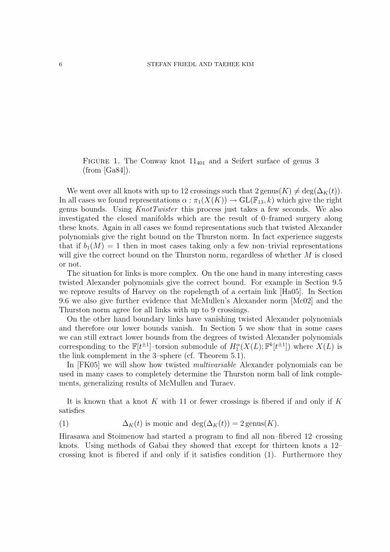
1.5. Examples. Consider the Conway knotK = 11401 (knotscape notation, cf. [HT]).The diagram is given in Figure 1. For this knot ∆K(t) = 1, therefore the genusbounds of McMullen, Turaev, Cochran and Harvey vanish. We found a representationα : π1(X(K)) → GL(F13, 4) such that deg (τ(M,φ, α)) = 14. These computationsand all the following computations were done using the program KnotTwister [F05].It follows from Theorem 3.1 that
2 genus(K)− 1 = ||φ||T ≥14
4.
Hence genus(K) ≥ 188
= 2.25. Since genus(K) is an integer we get genus(K) ≥ 3.Since there exists a Seifert surface of genus 3 for K (cf. Figure 1) it follows that thegenus of the Conway knot is 3. Gabai [Ga84] proved the same result using geometricmethods.
6 STEFAN FRIEDL AND TAEHEE KIM
Figure 1. The Conway knot 11401 and a Seifert surface of genus 3(from [Ga84]).
We went over all knots with up to 12 crossings such that 2 genus(K) 6= deg(∆K(t)).In all cases we found representations α : π1(X(K)) → GL(F13, k) which give the rightgenus bounds. Using KnotTwister this process just takes a few seconds. We alsoinvestigated the closed manifolds which are the result of 0–framed surgery alongthese knots. Again in all cases we found representations such that twisted Alexanderpolynomials give the right bound on the Thurston norm. In fact experience suggeststhat if b1(M) = 1 then in most cases taking only a few non–trivial representationswill give the correct bound on the Thurston norm, regardless of whether M is closedor not.
The situation for links is more complex. On the one hand in many interesting casestwisted Alexander polynomials give the correct bound. For example in Section 9.5we reprove results of Harvey on the ropelength of a certain link [Ha05]. In Section9.6 we also give further evidence that McMullen’s Alexander norm [Mc02] and theThurston norm agree for all links with up to 9 crossings.
On the other hand boundary links have vanishing twisted Alexander polynomialsand therefore our lower bounds vanish. In Section 5 we show that in some caseswe can still extract lower bounds from the degrees of twisted Alexander polynomialscorresponding to the F[t±1]–torsion submodule of Hα
1 (X(L); Fk[t±1]) where X(L) isthe link complement in the 3–sphere (cf. Theorem 5.1).
In [FK05] we will show how twisted multivariable Alexander polynomials can beused in many cases to completely determine the Thurston norm ball of link comple-ments, generalizing results of McMullen and Turaev.
It is known that a knot K with 11 or fewer crossings is fibered if and only if Ksatisfies
(1) ∆K(t) is monic and deg(∆K(t)) = 2 genus(K).
Hirasawa and Stoimenow had started a program to find all non–fibered 12–crossingknots. Using methods of Gabai they showed that except for thirteen knots a 12–crossing knot is fibered if and only if it satisfies condition (1). Furthermore they
THURSTON NORM, FIBERED MANIFOLDS AND TWISTED ALEXANDER POLYNOMIALS 7
showed that among these 13 knots the knots 121498, 121502, 121546 and 121752 are notfibered even though they satisfy condition (1).
Using Theorem 6.1 we confirmed the non–fiberedness of these 4 knots and weshowed that the remaining 9 knots are not fibered either. These 9 knots are:
121345, 121567, 121670, 121682, 121771, 121823, 121938, 122089, 122103.
This result completes the classification of all fibered 12–crossing knots. Jacob Ras-mussen confirmed our results using knot Floer homology which gives a fibering ob-struction as well (cf. [OS02, Section 3]).
As we pointed out our fibering obstructions work for closed manifolds as well. IfK is one of the 13 12–crossing knots in the previous paragraph, then we can easilyshow using Theorem 6.1 and KnotTwister that the zero surgery on K in S3 is notfibered. (See Section 9.2.)
1.6. Conjectures and symplectic manifolds. We propose the following conjec-ture.
Conjecture 10.1. Let M be a 3–manifold and φ ∈ H1(M) non–trivial. Then (M,φ)fibers over S1 if and only if for all epimorphisms α : π1(M) → G, G a finite group,the twisted Alexander polynomial ∆α
1 (t) ∈ Z[t±1] is monic and
||φ||T =1
|G|deg(τ(M,φ, α)).
We discuss this conjecture in detail in Section 10.6. We show that it holds in animportant case of satellite knots. We also show that it would follow from the ge-ometrization conjecture and the following conjecture.
Conjecture 10.5. Let S be an incompressible surface in M and let N be M cutalong S. Let i : S → N be one of the two canonical inclusions of S into N . Ifi∗ : Hα
1 (S; Z[G]) → Hα1 (N ; Z[G]) is surjective for every homomorphism π1(M) → G,
G a finite group, then i∗ : π1(S) → π1(N) is surjective.
Note that the inclusion induced homomorphisms π1(S) → π1(M) and π1(N) →π1(M) are clearly injections. Therefore Conjecture 10.5 becomes a conjecture in thetheory of 3–manifold groups.
Let M be a closed 3–manifold. Taubes conjectured that if S1 ×M is symplecticthen (M,φ) fibers over S1 for some φ ∈ H1(M). Vidussi [Vi99, Vi03] and Fintusheland Stern [FS98, p. 398] showed using work of Taubes [Ta94, Ta95] that if S1×M issymplectic then there exists φ ∈ H1(M) such that all abelian invariants of (M,φ) looklike invariants of fibered manifolds. In [FV05] the first author and Stefano Vidussiwill show that if S1×M is symplectic then there exists φ ∈ H1(M) such that (M,φ)satisfies the assumptions of Conjecture 10.1. This gives very strong evidence forTaubes’ conjecture and shows that Conjecture 10.1 implies Taubes’ conjecture.
8 STEFAN FRIEDL AND TAEHEE KIM
In Conjecture 10.6 we conjecture that twisted Alexander polynomials detect thegenus of hyperbolic knots. We show that this can also be reduced to a group theoreticproblem as in Conjecture 10.5.
1.7. Outline of the paper. In Section 2 we state some properties of the Thurstonnorm and give a definition of twisted Alexander polynomials. In Section 3 we stateTheorem 3.1 (Main Theorem 1) and discuss related theorems. We give a proof ofTheorem 3.1 in Section 4. In Section 5 we show how in many important cases we candrop the assumption that ∆α
1 (t) 6= 0 in Theorem 3.1 and still get lower bounds onthe Thurston norm. In Section 6 we consider fibered manifolds and give a proof ofTheorems 6.1 (Main Theorem 2) and 6.4. We formulate non–commutative versionsof Theorem 3.1 and Theorem 6.1 in Section 7. After showing in Section 8 how Foxcalculus can be used to efficiently compute twisted Alexander polynomials we discussa wealth of examples in Section 9. Finally in Section 10 we discuss and give furtherevidence for Conjectures 10.1 and related conjectures.
Notations and conventions: We assume that all 3–manifolds are compact, ori-ented and connected. All homology groups and all cohomology groups are with re-spect to Z–coefficients, unless it specifically says otherwise. For a knot K in S3, wedenote the result of zero framed surgery along K by MK . For a link L in S3, X(L)denotes the exterior of L in S3. (That is, X(L) = S3 \ νL where νL is an opentubular neighborhood of L in S3). An arbitrary (commutative) field is denoted byF. We identify the group ring F[Z] with F[t±1]. We denote the permutation groupof order k by Sk. For a 3–manifold M we use the canonical isomorphisms to iden-tify H1(M) = Hom(H1(M),Z) = Hom(π1(M),Z). Hence sometimes φ ∈ H1(M) isregarded as a homomorphism φ : π1(M) → Z (or φ : H1(M) → Z) depending on thecontext.
Acknowledgments: The authors would like to thank Alexander Stoimenow forproviding braid descriptions for the examples and Stefano Vidussi for pointing out theadvantages of using Reidemeister torsion. The first author would also like to thankJerry Levine for helpful discussions and he is indebted to Alexander Stoimenow forimportant feedback on the program KnotTwister.
2. The Thurston norm and twisted Alexander polynomials
2.1. The Thurston norm. For a connected CW complex X denote by χ(X) theEuler characteristic of X. We define χ−(X) := max{−χ(X), 0}. For a non-connectedCW complex X define χ−(X) =
∑χ−(Xi) where we sum over the connected com-
ponents of X. This is called the complexity of X. Now let M be a 3–manifold and

THURSTON NORM, FIBERED MANIFOLDS AND TWISTED ALEXANDER POLYNOMIALS 9
φ ∈ H1(M). Then we define
||φ||T,M := min{χ−(S)},where we take the minimum with respect to all properly embedded surfaces S whichare dual to φ. Note that we take the minimum over a non–empty set since any φ isdual to a properly embedded surface (cf. [Th86]). If the manifold M is clear we willjust write ||φ||T .Thurston [Th86] introduced || − ||T,M in a preprint in 1976 and proved the followingtheorem (cf. [Oe86] [Kr98]) which justifies the name Thurston norm.
Theorem 2.1. (1) For φ, φ1, φ2 ∈ H1(M) and k ∈ N we have the following:
||kφ||T = k||φ||T ,||φ1 + φ2||T ≤ ||φ1||T + ||φ2||T .
(2) There exists a seminorm || − ||T on H1(M ; R) which equals || − ||T on theintegral lattice H1(M).
(3) If no element in H1(M) is dual to an embedded surface of non–negative Eulercharacteristic, then ||− ||T is in fact a norm. In particular if M is hyperbolic,then || − ||T is a norm.
(4) The unit ball of the Thurston norm is a finite, convex, possibly non–compactpolyhedron.
Proof. (1) We refer to [Th86].(2) It is now easy to see that the convex function ||−||T onH1(M) can be extended
to a seminorm || − ||T on H1(M ; R) (cf. [Th86, p. 104] for details).(3) This follows immediately from the definition and from Thurston’s hyperbol-
icity theorem (cf. [Th82]).(4) We refer to [Th86, Theorem 2].
�
As an illustration we outline the proof of the following lemma. At several lateroccasions we will make use of the arguments in this proof.
Lemma 2.2. Let K ⊂ S3 be a non–trivial knot and φ ∈ H1(X(K)) a generator.Then ||φ||T = 2 genus(K)− 1.
Proof. Clearly a Seifert surface for K is dual to φ, hence ||φ||T ≤ 2 genus(K) − 1.Denote the longitude of K by λ. If S is dual to φ with minimal complexity, then∂S = [λ] ∈ H1(K×S1) (we identify ∂X(K) with K×S1). Note that every boundarycomponent of S is essential in K × S1. Otherwise we can find an innermost circlewhich bounds a disk, which can then be attached to find a dual surface of lowercomplexity.
Therefore each component of ∂S is non–trivial in H1(K × S1). Since at least onecomponent of ∂S represents [λ] ∈ H1(K × S1) it follows that in fact each componentof ∂S represents ±[λ] since the components are disjoint. In particular it follows
10 STEFAN FRIEDL AND TAEHEE KIM
that ∂S has an odd number of components. If ∂S has 2k + 1 components, then totwo adjacent components of ∂S with opposite orientations we can attach an annulusand push this part off the boundary of X(K). Note that adding an annulus doesnot change the complexity. Repeating this process gives a possibly disconnectedsurface. One component is a Seifert surface F for K, and the remaining componentsare closed. Since we can throw away the closed components it now follows that||φ||T = b1(F )− 1 ≥ 2 genus(K)− 1. �
Strictly speaking the Thurston norm is not a norm, but only a seminorm. Forexample if M = S1×S1×S1, then clearly every element in H2(M) is represented bya disjoint union of tori, hence the Thurston norm vanishes completely on H1(M).
2.2. Alexander polynomials. Let M be a 3–manifold and φ ∈ H1(M). Let α :π1(M) → GL(F, k) be a representation. We can now define a left Z[π1(M)]–modulestructure on Fk ⊗F F[t±1] =: Fk[t±1] via α⊗ φ as follows:
g · (v ⊗ p) := (α(g) · v)⊗ (φ(g) · p) = (α(g) · v)⊗ (tφ(g)p)
where g ∈ π1(M), v ⊗ p ∈ Fk ⊗F F[t±1] = Fk[t±1].Denote by M the universal cover of M . Then the chain groups C∗(M) are in
a natural way right Z[π1(M)]–modules. Therefore we can form the tensor productC∗(M)⊗Z[π1(M)]Fk[t±1]. Now we define the i–th twisted Alexander module of (M,φ, α)to be
Hα⊗φ∗ (M ; Fk[t±1]) := H∗(C∗(M)⊗Z[π1(M)] Fk[t±1]).
Usually we drop the notation φ and write Hα∗ (M ; Fk[t±1]). Note that Hα
i (M ; Fk[t±1])is a finitely generated module over the PID F[t±1]. Therefore there exists an isomor-phism
Hαi (M ; Fk[t±1]) ∼= F[t±1]f ⊕
k⊕i=1
F[t±1]/(pi(t))
for p1(t), . . . , pk(t) ∈ F[t±1]. We define
∆αM,φ,i :=
{ ∏ki=1 pi(t), if f = 0
0, if f > 0.
This is called the i–th twisted Alexander polynomial of (M,φ, α). We furthermore
define ∆αM,φ,i :=
∏ki=1 pi(t) regardless of f . In most cases we drop the notations M
and φ and write ∆αi (t) and ∆α
i (t). It follows from the structure theorem of finitelygenerated modules over a PID that these polynomials are well–defined up to multi-plication by a unit in F[t±1]. In Section 8 we will see that ∆α
i (t) and ∆αi (t) can be
computed easily for i = 0, 1 given a presentation of π1(M).
Remark. The first twisted Alexander polynomial for a knot was originally defined byLin in 1990 using a presentation of the fundamental group [Lin01]. This was general-ized by Jiang and Wang [JW93] and the multivariable twisted Alexander polynomial
THURSTON NORM, FIBERED MANIFOLDS AND TWISTED ALEXANDER POLYNOMIALS 11
was first introduced by Wada [Wa94] given only a presentation of a group and arepresentation to GL(R, k) where R is a UFD. Wada’s definition differs slightly fromour definition even in the case that it is associated to a representation to Z. Ourhomological definition of twisted Alexander polynomials in the above was originallyintroduced by Kirk and Livingston in [KL99a].
For an oriented knotK we always assume that φ denotes the generator ofH1(X(K))given by the orientation. If α : π1(X(K)) → GL(Q, 1) is the trivial representa-tion then the Alexander polynomial ∆α
1 (t) equals the classical Alexander polynomial∆K(t) ∈ Q[t±] of the knot K.
Remark. When K is a knot, then the untwisted homology H1(X(K); F[t±1]) is F[t±1]–torsion. But even for a knot complement it can happen that in the twisted caseHα
1 (X(K); Fk[t±1]) is not F[t±1]–torsion (cf. e.g. [KL99a]).
If f = 0 then we write deg(f) = ∞, otherwise, for f =∑n
i=m aiti ∈ F[t±1] with
am 6= 0, an 6= 0 we define deg(f) = n−m. Note that deg (∆αi (t)) is well–defined. The
following observation follows immediately from the classification theorem of finitelygenerated modules over a PID.
Lemma 2.3. Hαi (M ; Fk[t±1]) is a finite–dimensional F–vector space if and only if
∆αi (t) 6= 0. If ∆α
i (t) 6= 0, then
deg (∆αi (t)) = dimF
(Hαi (M ; Fk[t±1])
).
Furthermore deg(∆αi (t)) = dimF
(TorF[t±1](H
αi (M ; Fk[t±1]))
).
If ∂M is empty or consists of tori and if ∆α1 (t) 6= 0, then ∆α
i (t) 6= 0 for all i andhence Hα
i (M ; Fk[t±1] ⊗F[t±1] F(t)) = 0 for all i (see Corollary 4.3). Therefore theReidemeister torsion τ(M,φ, α) ∈ F(t) is defined. We refer to [Tu01] for an excellentintroduction into the theory of Reidemeister torsion. τ(M,φ, α) ∈ F(t) is well–defined
up to multiplication by an element of the form rtk, r ∈ Im{π1(M)α−→ GL(F, k) det−→ F}.
We will not make use of this, and mostly use τ(M,φ, α) as a convenient way to storeinformation.
Lemma 2.4. (cf. [Tu01, p. 20]) If ∆α1 (t) 6= 0, then τ(M,φ, α) is defined and
τ(M,φ, α) =3∏i=0
∆αi (t)
(−1)i+1 ∈ F(t).
3. Main Theorem 1: Lower bounds on the Thurston norm
3.1. Statement of Main Theorem 1. Our main theorem gives a lower bound forthe Thurston norm of a non–trivial element φ ∈ H1(M).

12 STEFAN FRIEDL AND TAEHEE KIM
Theorem 3.1 (Main Theorem 1). Let M be a 3–manifold whose boundary is emptyor consists of tori. Let φ ∈ H1(M) be non–trivial and let α : π1(M) → GL(F, k) be arepresentation such that ∆α
1 (t) 6= 0. Then
||φ||T ≥ 1k
deg(τ(M,φ, α))
= 1k
(deg (∆α
1 (t))− deg (∆α0 (t))− deg (∆α
2 (t))).
The proof of the above theorem is given in Section 4. In Section 8 we will show howto compute ∆α
1 (t) and ∆α0 (t) using a presentation of π1(M). In Section 4.4 we will
also give a proof of the following proposition which allows us to compute ∆α2 (t) using
the algorithm for computing the 0-th twisted Alexander polynomial.Assume that F has a (possibly trivial) involution. Let 〈 , 〉 be the canonical her-
mitian inner product on Fk. Then there exists a unique representation α : π1(M) →GL(F, k) such that
〈α(g−1)v, w〉 = 〈v, α(g)w〉for all g ∈ π1(M) and v, w ∈ Fk.Proposition 3.2. Let M be a 3–manifold whose boundary is empty or consists of toriand let φ ∈ H1(M) be non–trivial. Let α : π1(M) → GL(F, k) be a representationsuch that ∆α
1 (t) 6= 0.
(1) If M is closed, then∆α
2 (t) = ∆α0 (t−1).
(2) If M has non–empty boundary, then ∆α2 (t) = 1.
In particulardeg (∆α
2 (t)) = b3(M) deg(∆α
0 (t)).
For a unitary representation we have α = α, therefore we get the following impor-tant special case of Theorem 3.1:
Theorem 3.3. Let M be a 3–manifold whose boundary is empty or consists of tori.Let φ ∈ H1(M) be non–trivial and let α : π1(M) → GL(F, k) be a unitary represen-tation such that ∆α
1 (t) 6= 0. Then
||φ||T ≥1
k
(deg (∆α
1 (t))−(1 + b3(M)
)deg (∆α
0 (t))).
Remark. (1) Our restriction to closed manifolds or manifolds whose boundaryconsists of tori is not a significant restriction. Indeed, if ∂M has a sphericalboundary component, then gluing in a 3–ball does not change the Thurstonnorm. Furthermore manifolds with a boundary component of genus greaterthan 1 have in most cases vanishing twisted Alexander polynomials.
(2) We point out that a slightly different proof of Theorem 3.1 shows that in fact
Theorem 3.3 holds for all 3–manifolds if we replace b3(M) by b3(M) where
we define b3(M) = 1 if M is closed or if the boundary of M consists only of
spheres, and b3(M) = 0 otherwise.
THURSTON NORM, FIBERED MANIFOLDS AND TWISTED ALEXANDER POLYNOMIALS 13
The following lemma shows that in most cases we can determine for a given φ ∈H1(M) whether ||φ||T is even or odd. This means that we can ‘round up’ the lowerbounds from Theorem 3.1 to an even or odd number, depending on the parity of ||φ||T .Recall that for a non–trivial φ ∈ H1(M) the divisibility of φ equals the maximumnatural number n such that 1
nφ ∈ H1(M).
Lemma 3.4. Let φ ∈ H1(M) be primitive. If M is closed, then ||φ||T is even. Assumethat ∂M consists of a non–empty collection of tori N1 ∪ · · · ∪Ns. If φ|H1(Ni) = 0 thenlet ni := 0, otherwise define ni to be the divisibility of φ|H1(Ni). Then
||φ||T ≡( s∑
i=1
ni
)mod 2.
Proof. Let S be a properly embedded surface dual to φ with minimal complexity. IfM is closed then S is closed, hence χ(S) is even. Now assume that ∂M is a collectionof tori. Then
χ−(S) ≡ b0(∂S) mod 2.
This follows from the observation that adding a 2–disk to each component of ∂Sgives a closed surface, which has even Euler characteristic. Now consider Ni. ClearlyS ∩ Ni is Poincare dual to φ|H1(Ni). It follows from an argument as in Lemma 2.2that, modulo 2, ∂S ∩Ni has ni components. �
In Section 9.2 we will see that Theorem 3.1 can be very successfully used to deter-mine the genus of knots and the Thurston norm of closed manifolds. In particular wegive many examples of triples (M,φ ∈ H1(M), α : π1(M) → GL(F, k)) for which
b(M,φ, α) := 1k
(deg (∆α
1 (t))− deg (∆α0 (t))− deg (∆α
2 (t)))
> b(M,φ) := deg(∆1(t))− deg(∆0(t))− deg(∆2(t)),
i.e., we have many examples where the degrees of twisted Alexander polynomials givebetter bounds on the Thurston norm than the degree of the untwisted Alexanderpolynomial. In most cases we have b(M,φ, α) ≥ b(M,φ). But if we take K to be theknot 94, φ a generator of H1(X(K)), then there exists a map α : π1(X(K)) � S3 →GL(Q, |S3|) with deg (∆α
0 (t)) = 2, and such that
∆α1 (t) = 9− 13t2 − 8t4 + 24t6 − 8t8 − 13t10 + 9t12 ∈ Q[t±1].
Since ∆1(t) = 3− 5t+ 5t2 − 5t3 + 3t4 it follows that
b(M,φ, α) =5
3< 3 = b(M,φ).
This example shows that twisted Alexander polynomials give at times bounds onthe Thurston norm that are worse than the bounds from the ordinary Alexanderpolynomials. This should be compared to the situation of [Co04] (cf. also [Ha06]) :Cochran’s sequence of higher order Alexander polynomials gives a never decreasing
14 STEFAN FRIEDL AND TAEHEE KIM
sequence of lower bounds on the genus of a knot.
In the following sections we discuss several interesting types of representationswhich allow us to recover work of McMullen [Mc02] and Turaev [Tu02b].
3.2. The trivial representation: McMullen’s theorem. If we let α : π1(M) →GL(F, 1) be the trivial representation then given any primitive φ ∈ H1(M) we have
Hα0 (M ; F[t±1]) ∼= F[t±1]/{tif − f |i ∈ Z, f ∈ F[t±1]} ∼= F[t±1]/(t− 1).
Therefore ∆0(t) = t − 1. Since the trivial representation is unitary we immediatelyget McMullen’s theorem from Theorem 3.3:
Theorem 3.5. [Mc02, Proposition 6.1] Let M be a 3–manifold whose boundary isempty or consists of tori and φ ∈ H1(M) primitive. If ∆1(t) 6= 0, then for any fieldF
||φ||T ≥ deg(∆1(t))−(1 + b3(M)
).
In fact McMullen showed more: he introduced a norm || − ||A on H1(M ; R), calledthe Alexander norm, and showed that if b1(M) > 1 then
||φ||T ≥ ||φ||A
for all φ ∈ H1(M ; R). Furthermore ||φ||A ≥ deg(∆1(t))−1−b3(M) for all φ ∈ H1(M),and equality holds for almost all φ ∈ H1(M). In [FK05] the authors will introducetwisted Alexander norms which give lower bounds on the Thurston norm, extendingthe work of McMullen and Turaev [Tu02a].
3.3. Abelian representations: Turaev’s theorem. The following was first shownby Turaev [Tu02a].
Theorem 3.6. Let M be a 3–manifold whose boundary is empty or consists of tori,φ ∈ H1(M) primitive, and α : π1(M) → H1(M) → GL(F, 1) a one–dimensionalrepresentation which is non–trivial on Ker(φ). If ∆α
1 (t) 6= 0, then
||φ||T ≥ deg (∆α1 (t)) .
Proof. Let β : π1(M) → GL(F, 1) be a representation. Using that φ : π1(M) → Z issurjective one can easily show that
Hβ0 (M ; F[t±1]) ∼= F[t±1]/{β(g)tφ(g)f − f | g ∈ π1(M), f ∈ F[t±1]} ∼= F
if β is trivial on Ker(φ), and Hβ0 (M ; F[t±1]) = 0 otherwise. We apply this to
Hα0 (M ; F[t±1]) and Hα
0 (M ; F[t±1]). Turaev’s theorem now follows from Theorem 3.1and Proposition 3.2. �
THURSTON NORM, FIBERED MANIFOLDS AND TWISTED ALEXANDER POLYNOMIALS 15
This simple abelian version of Theorem 3.1 can already be very useful. Using resultsof [FK05] one can show that for primitive φ ∈ H1(M)
||φ||A = max{deg (∆α1 (t)) |α : π1(M) → H1(M)/Tor(H1(M)) → GL(C, 1)
non–trivial on Ker(φ)},where ||φ||A denotes McMullen’s Alexander norm. Harvey [Ha05, Proposition 3.12]showed that the invariant δ0(φ) in [Ha05] equals ||φ||A. This shows that Alexan-der polynomials corresponding to one–dimensional representations contain all knownlower bounds on the Thurston norm coming from abelian covers.
3.4. Finite covers. LetM be a 3–manifold, φ ∈ H1(M) non–trivial and α : π1(M) →G a homomorphism to a finite group. Then we get a representation α : π1(M) →G → GL(F, |G|) via the regular representation of G. In Section 9.1 we will see thatthis gives an abundant supply of representations. We denote the resulting Alexanderpolynomials by ∆G
i (t), suppressing the homomorphism α in the notation.
Theorem 3.7. Let M be a 3–manifold whose boundary is empty or consists of tori,φ ∈ H1(M) primitive, and α : π1(M) → G an epimorphism to a finite group. If∆G
1 (t) 6= 0 then
||φ||T ≥1
|G|(deg
(∆G
1 (t))−
(1 + b3(M)
)deg
(∆G
0 (t))).
Since the representation α : π1(M) → G → GL(F, |G|) is unitary, Theorem 3.7follows from Theorem 3.3. We outline an illuminating alternative proof of Theorem3.7, using only McMullen’s Theorem 3.5. Let M be a 3–manifold and α : π1(M) → Ga homomorphism to a finite group G. We denote the induced G–cover of M by MG.For φ : H1(M) → Z we denote the induced map H1(MG) → H1(M) → Z by φG.Note that if φ : H1(M) → Z is non–trivial, then φG is non–trivial as well.
Lemma 3.8.|G| · ||φ||T,M = ||φG||T,MG
∆GM,φ,i(t) = ∆MG,φG,i(t), for all i
.
For the second part we refer to [FV05]. The first part was shown by Gabai [Ga83]. Infact we will only need the inequality |G|·||φ||T,M ≥ ||φG||T,MG
which can easily be seendirectly using the fact that if SG is the G–cover of a surface S, then χ(SG) = |G|χ(S).
Alternative proof of Theorem 3.7. It is easy to see that φ(Ker(α)) 6= 0. Thereforewe can define n ∈ N to be the divisibility of φ restricted to Ker(α). Recall that
φG is given by H1(MG) ∼= H1(Ker(α)) → H1(M)φ−→ Z. It follows that the element
1nφG ∈ H1(MG) is defined and primitive. Since α is an epimorphism, MG is connected
and we can apply Theorem 3.5 to conclude that∣∣∣∣ 1nφG
∣∣∣∣T,MG
≥ deg(∆MG,
1nφG,1
(t))−
(1 + b3(M)
)= deg
(∆MG,
1nφG,1
(t))−
(1 + b3(M)
)deg
(∆MG,
1nφG,0
(t)).
16 STEFAN FRIEDL AND TAEHEE KIM
The second equality follows from the observation that ∆MG,1nφG,0
(t) = t − 1. By
Lemma 3.8 and the homogeneity of the Thurston norm we get
|G| · ||φ||T,M = ||φG||T,MG
= n∣∣∣∣ 1nφG
∣∣∣∣T,MG
≥ n(deg
(∆MG,
1nφG,1
(t))−
(1 + b3(M)
)deg
(∆MG,
1nφG,0
(t))).
Clearly ∆MG,φG,i(t) = ∆MG,1nφG,i
(tn). Therefore n deg(∆MG,
1nφG,i
(t))
= deg(∆MG,φG,i(t)
).
The theorem now follows immediately from Lemma 3.8. and the observation thatb3(MG) = b3(M). �
4. Proof of Main Theorem 1
4.1. Twisted Alexander polynomials of (M,φ).
Lemma 4.1. Let φ ∈ H1(M) be non–trivial and α : π1(M) → GL(F, k) a repre-sentation. Then Hα
3 (M ; Fk[t±1]) = 0 and Hα0 (M ; Fk[t±1]) is finite dimensional as a
F–vector space.
Proof. First assume that M is closed. We make use of an argument in the proof of[Mc02, Theorem 5.1]. Choose a triangulation τ of M . Let T be a maximal tree inthe 1-skeleton of τ and let T ′ be a maximal tree in the dual 1-skeleton. We collapseT to form a single 0-cell and join the 3-simplices of T ′ to form a single 3-cell. Denotethe number of 1-cells by n. It follows from M closed that χ(M) = 0, hence there aren 2-cells.
Write π := π1(M). From the CW structure we obtain a chain complex C∗ := C∗(M)
0 → C13
∂3−→ Cn2
∂2−→ Cn1
∂1−→ C10 → 0
where the Ci are free Z[π]-right modules. In fact Cki∼= Z[π]k. Let Ai, i = 0, . . . , 3, be
the matrices with entries in Z[π] corresponding to the boundary maps ∂i : Ci → Ci−1
with respect to the bases given by the lifts of the cells of M to M . Then we canarrange the lifts such that
A3 = (1− g1, 1− g2, . . . , 1− gn)t,
A1 = (1− h1, 1− h2, . . . , 1− hn),
where {g1, . . . , gn} and {h1, . . . , hn} are generating sets for π1(M). Consider the chaincomplex C∗ ⊗Z[π] Fk[t±1]
0 → C13⊗Z[π]Fk[t±1]
∂3⊗id−−−→ Cn2⊗Z[π]Fk[t±1]
∂2⊗id−−−→ Cn1⊗Z[π]Fk[t±1]
∂1⊗id−−−→ C10⊗Z[π]Fk[t±1] → 0.
Let B = (brs) be a p × q matrix with entries in Z[π]. We write brs =∑bgrsg for
bgrs ∈ Z, g ∈ π. We define (α⊗φ)(B) to be the p×q matrix with entries∑bgrsα(g)tφ(g).
Since each∑bgrsα(g)tφ(g) is a k × k matrix with entries in F[t±1] we can think of
(α⊗ φ)(B) as a pk × qk matrix with entries in F[t±1].
THURSTON NORM, FIBERED MANIFOLDS AND TWISTED ALEXANDER POLYNOMIALS 17
Note that ∂i ⊗ id is represented by (α ⊗ φ)(Ai). Since φ is non-trivial there existk, l such that φ(gk) 6= 0 and φ(hl) 6= 0. It follows that (α ⊗ φ)(A1) and (α ⊗ φ)(A3)have full rank over F[t±1]. The lemma now follows immediately in the case that Mis closed.
IfM has boundary, then clearlyHα3 (M ; Fk[t±1]) = 0. The argument thatHα
0 (M ; Fk[t±1])is finite dimensional is exactly the same as in the closed case. �
We note that the fact that Hα0 (M ; Fk[t±1]) is finite–dimensional was first proved
by Kirk and Livingston in [KL99a, Proposition 3.5].
Lemma 4.2. Assume that ∂M is empty or consists of tori and φ ∈ H1(M) isnon–trivial. Let α : π1(M) → GL(F, k) be a representation. If ∆α
1 (t) 6= 0, thenHα
2 (M ; Fk[t±1]) is F[t±1]–torsion. In particular ∆α2 (t) 6= 0.
Proof. We know that ∆αi (t) 6= 0 for i = 0, 1, 3 by assumption and by Lemma 4.1. It
follows from the long exact homology sequence for (M,∂M) and from duality thatχ(M) = 1
2χ(∂M). Hence χ(M) = 0 in our case. It follows from Lemma 4.14 (applied
to the field F(t)) that
3∑i=0
(−1)idimF(t)
(Hαi (M ; Fk[t±1]⊗F[t±1] F(t))
)= k · χ(M) = 0.
Note that Hαi (M ; Fk[t±1] ⊗F[t±1] F(t)) = Hα
i (M ; Fk[t±1]) ⊗F[t±1] F(t) since F(t) isflat over F[t±1]. By assumption Hα
i (M ; Fk[t±1]) ⊗F[t±1] F(t) = 0 for i 6= 2, henceHα
2 (M ; Fk[t±1])⊗F[t±1] F(t) = 0 by Lemma 4.14. �
We get the following corollary immediately from Lemmas 4.1 and 4.2.
Corollary 4.3. Let M be a 3–manifold whose boundary is empty or consists of tori.Let φ ∈ H1(M) be non–trivial and α : π1(M) → GL(F, k) a representation. If∆α
1 (t) 6= 0 then ∆αi (t) 6= 0 for all i, and ∆α
3 (t) = 1.
4.2. Main argument. In this section we prove Theorem 3.1. Before beginning theproof we give relevant propositions and lemmas. In an attempt to make the proofeasier to read we prove several technical lemmas separately in Section 4.3. We alsoneed one delicate duality argument which we explain in detail in Section 4.4
Let M be a 3–manifold and α : π1(M) → GL(F, k) a representation. We will endow
any subset X ⊂ M with the representation given by π1(X) → π1(M)α−→ GL(F, k).
Note that because of base point issues this induced homomorphism is only defined upto conjugacy. But the homology groups Hα
∗ (X; Fk) are isomorphic, and their dimen-sions over F are well-defined. We will therefore suppress base points and the choiceof paths connecting base points in our notation. Let bαn(X) := dimF(H
αn (X; Fk)) for
n ≥ 0.
18 STEFAN FRIEDL AND TAEHEE KIM
Proposition 4.4. Let φ ∈ H1(M) and S a properly embedded surface dual to φ.Then
bα1 (S) ≥ dimF(TorF[t±1]
(Hα
1 (M ; Fk[t±1]))).
In particular if ∆α1 (t) 6= 0, then bα1 (S) ≥ deg (∆α
1 (t)).
Proof. Denote the components of S by S1, . . . , Sl. Denote by N the result of cuttingM along S. Denote by i+ and i− the two inclusions of S into ∂N induced by takingthe positive and the negative inclusions of S into N . We use the same notations i+and i− for the induced homomorphisms on homology groups. Note that φ vanisheson π1(N) and on every π1(Si). Indeed, every curve in Si can be pushed off intoN , where φ vanishes. It follows that Hα
i (N ; Fk[t±1]) ∼= Hαi (N ; Fk) ⊗F F[t±1] and
Hαi (S; Fk[t±1]) ∼= Hα
i (S; Fk) ⊗F F[t±1]. Therefore we have a commutative diagram ifexact sequences(2)
→ Hαi (S; Fk[t±1])
ti−−i+−−−−→ Hαi (N ; Fk[t±1]) → Hα
i (M ; Fk[t±1]) →↓∼= ↓∼= ↓= →
→ Hαi (S; Fk)⊗F F[t±1]
ti−−i+−−−−→ Hαi (N ; Fk)⊗F F[t±1] → Hα
i (M ; Fk[t±1]). →
Note that Ker{Hα0 (S; Fk[t±1]) → Hα
0 (N ; Fk[t±1])} ⊂ Hα0 (S; Fk)⊗FF[t±1] is a (possibly
trivial) free F[t±1]–module F . Therefore we get an exact sequence
Hα1 (S; Fk)⊗F F[t±1]
ti−−i+−−−−→ Hα1 (N ; Fk)⊗F F[t±1] → Hα
1 (M ; Fk[t±1])∂−→ F → 0.
Since F[t±1] is a PID the map ∂ splits, i.e., Hα1 (M ; Fk[t±1]) ∼= Ker(∂) ⊕ F . Using
appropriate bases the map ti−− i+, which represents the module Ker(∂), is presentedby a matrix of size dimF
(Hα
1 (N ; Fk))× dimF
(Hα
1 (S; Fk))
of the form At + B, A,Bmatrices over F. It follows from Lemma 4.10 that
bα1 (S) = dimF(Hα
1 (S; Fk))≥ dimF
(TorF[t±1](H
α1 (M ; Fk[t±1]))
).
The last part of this proposition is obvious by Lemma 2.3. �
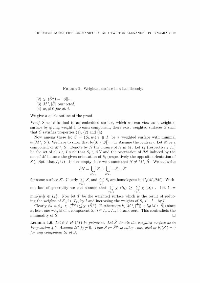
A weighted surface S in M is a collection of pairs (Si, wi), i = 1, . . . , k whereSi ⊂ M are properly embedded, oriented, disjoint surfaces in M and wi are non–negative integers. We denote the union
⋃i,wi 6=0 Si ⊂M by |S|.
Every weighted surface S defines an element φS :=∑k
i=1wi · PD([Si]) ∈ H1(M)where PD(f) ∈ H1(M) denotes the Poincare dual of an element f ∈ H2(M,∂M).By taking wi parallel copies of Si we get an (unweighted) properly embedded orientedsurface S# such that φS = PD(S#). An example of a the surface S# for a weighted
surface S is given in Figure 2.We need the following proposition proved by Turaev in [Tu02b].
Proposition 4.5. Let φ ∈ H1(M). Then there exists a weighted surface S with
(1) φS = φ,
THURSTON NORM, FIBERED MANIFOLDS AND TWISTED ALEXANDER POLYNOMIALS 19
Figure 2. Weighted surface in a handlebody.
(2) χ−(S#) = ||φ||T ,(3) M \ |S| connected,(4) wi 6= 0 for all i.
We give a quick outline of the proof.
Proof. Since φ is dual to an embedded surface, which we can view as a weightedsurface by giving weight 1 to each component, there exist weighted surfaces S suchthat S satisfies properties (1), (2) and (4).
Now among these let S = (Si, wi), i ∈ I, be a weighted surface with minimalb0(M \ |S|). We have to show that b0(M \ |S|) = 1. Assume the contrary. Let N be acomponent of M \ |S|. Denote by N the closure of N in M . Let I+ (respectively I−)be the set of all i ∈ I such that Si ⊂ ∂N and the orientation of ∂N induced by theone of M induces the given orientation of Si (respectively the opposite orientation ofSi). Note that I+∪I− is non–empty since we assume that N 6= M \ |S|. We can write
∂N =⋃i∈I+
Si ∪⋃i∈I−
−Si ∪ S ′
for some surface S ′. Clearly∑i∈I+
Si and∑i∈I−
Si are homologous in C2(M,∂M). With-
out loss of generality we can assume that∑i∈I+
χ−(Si) ≥∑i∈I−
χ−(Si) . Let l :=
min{wi|i ∈ I+}. Now let T be the weighted surface which is the result of reduc-ing the weights of Si, i ∈ I+, by l and increasing the weights of Si, i ∈ I−, by l.
Clearly φT = φS, χ−(T#) ≤ χ−(S#). Furthermore b0(M \ |T |) < b0(M \ |S|) sinceat least one weight of a component Si, i ∈ I+∪ I−, became zero. This contradicts theminimality of S. �
Lemma 4.6. Let φ ∈ H1(M) be primitive. Let S denote the weighted surface as inProposition 4.5. Assume ∆α
1 (t) 6= 0. Then S := S# is either connected or bα0 (Si) = 0for any component Si of S.

20 STEFAN FRIEDL AND TAEHEE KIM
Proof. Denote by N the result of cutting M along S. Consider the Mayer–Vietorissequence (2) in Proposition 4.4
→ Hα1 (M ; Fk[t±1])
→ Hα0 (S; Fk)⊗F F[t±1]
ti−−i+−−−−→ Hα0 (N ; Fk)⊗F F[t±1] → Hα
0 (M ; Fk[t±1]) → 0.
From ∆α1 (t) 6= 0 it follows that Hα
1 (M ; Fk[t±1]) is F[t±1]–torsion. By Lemma 4.1Hα
0 (M ; Fk[t±1]) is a finite–dimensional F–vector space, hence F[t±1]–torsion. If wenow consider the above exact sequence with F(t)–coefficients it follows that
(3) H0(S; Fk) ∼= H0(N ; Fk).Since we can arrange wi parallel copies of Si inside ν(Si) in M , we see that N ∼=
(M \ ν|S|) ∪l⋃
i=1
wi−1⋃j=1
Si × [−1, 1]. Therefore we have the following isomorphisms
(4)Hα
0 (S; Fk) ∼=l⊕
i=1
Hα0 (Si; Fk) ⊕
l⊕i=1
Hα0 (Si; Fk)wi−1
Hα0 (N ; Fk) ∼= Hα
0 (M \ ν|S|; Fk) ⊕l⊕
i=1
Hα0 (Si; Fk)wi−1
where Hα0 (Si; Fk)wi−1 :=
wi−1⊕Hα
0 (Si; Fk). Note that the maps i+, i− : π1(Si) →π1(M)
α−→ GL(F, k) factor through π1(M \ ν|S|). Therefore
(5) bα0 (Si) ≥ bα0 (M \ ν|S|), i = 1, . . . , l
by Lemma 4.13.First consider the case bα0 (M \ ν|S|) = 0. In that case it follows from the isomor-
phisms in (3) and (4) thatl⊕
i=1
H0(Si; Fk) = 0, hence bα0 (Si) = 0 for all i = 1, . . . , l.
Now assume that bα0 (M \ ν|S|) > 0. It follows immediately from the isomorphismsin (3) and (4) and from the inequality (5) that l = 1. But since φ is primitive it alsofollows that w1 = 1, i.e., S is connected. �
Lemma 4.7. Let φ ∈ H1(M) be primitive and ∆α1 (t) 6= 0. Let S := S# denote the
same surface as in Proposition 4.5. Then
bα0 (S) = deg (∆α0 (t)) .
Proof. Let N be M cut along S. Since ∆α1 (t) 6= 0, we have Hα
0 (S; Fk) ∼= Hα0 (N ; Fk)
as F–vector spaces (see (2) in the proof of Lemma 4.6). First assume that bα0 (Si) = 0for every component Si of S. Then Hα
0 (S; Fk) = Hα0 (N ; Fk) = 0. This implies that
Hα0 (M ; Fk[t±1]) = 0 from the exact sequence (2) in the proof of Proposition 4.4, hence
∆α0 (t) = 1.Now assume that bα0 (Si) 6= 0 for some i. By Lemma 4.6 S is connected. Hence
N is connected. It follows from Lemma 4.13 that the maps i+, i− : Hα0 (S; Fk) →
THURSTON NORM, FIBERED MANIFOLDS AND TWISTED ALEXANDER POLYNOMIALS 21
Hα0 (N ; Fk) are surjective. Since Hα
0 (S; Fk) ∼= Hα0 (N ; Fk) it follows that i+ and i−
induce isomorphisms on Hα0 (S; Fk). Note that this argument uses that S is connected.
Let b := bα0 (S) = bα0 (N). Picking appropriate bases for Hα0 (S; Fk) and Hα
0 (N ; Fk)the sequence (2) becomes
Fb ⊗F F[t±1]t·Id−J−−−−→ Fb ⊗F F[t±1] → Hα
0 (M ; Fk[t±1]) → 0,
where J : Fb → Fb is an isomorphism. It follows that Hα0 (M ; Fk[t±1]) ∼= Fb ∼=
Hα0 (S; Fk). The lemma now follows from Lemma 2.3. �
We note that from Lemmas 4.6 and 4.7 we immediately get the following usefulcorollary:
Corollary 4.8. If ∆α0 (t) 6= 1 and ∆α
1 (t) 6= 0, then there exists a surface of minimalcomplexity dual to φ which is connected.
Lemma 4.9. Assume that ∂M is empty or consists of tori. Let φ ∈ H1(M) beprimitive and ∆α
1 (t) 6= 0. Let S := S# denote the same surface as in Proposition 4.5.Then
bα2 (S) = deg (∆α2 (t)) .
Proof. Let S = (Si, wi)i=1,...,l be the weighted surface with wi 6= 0 for all i from
Proposition 4.5. Let N be M cut along S = S#. Let I ′ := {i ∈ {1, . . . , l}|Si closed}and I ′′ := {i ∈ {1, . . . , l}|Si has non–empty boundary}. Denote the union of wiparallel copies of Si, i ∈ I ′, by S ′ ⊂ S. Clearly bα2 (S) = bα2 (S ′).
Note that we can write ∂N = S ′+ ∪ S ′
− ∪ W for some surface W where S ′− and
S ′+ are the images of the two canonical inclusion maps of S ′ → N . It follows from
Lemmas 4.1 and 4.2 that the long exact sequence (2) becomes
0 → Hα2 (S ′; Fk)⊗F F[t±1]
ti−−i+−−−−→ Hα2 (N ; Fk)⊗F F[t±1] → Hα
2 (M ; Fk[t±1]) → 0.
Clearly we are done once we show that i−, i+ : Hα2 (S ′; Fk) → Hα
2 (N ; Fk) are isomor-phisms. Considering the sequence with F(t)–coefficients it follows thatHα
2 (S ′; Fk) andHα
2 (N ; Fk) have the same dimension as F-vector spaces. It is therefore enough to showthat i− and i+ are injections, or equivalently that the maps Hα
2 (S ′±; Fk) → Hα
2 (N ; Fk)are injections.
Consider the short exact sequence
Hα3 (N,S+; Fk) → Hα
2 (S ′+; Fk) → Hα
2 (N ; Fk).
By Poincare duality and by Lemma 4.15 we have
Hα3 (N,S ′
+; Fk) ∼= H0α(N,S
′− ∪W ; Fk) ∼= HomF(H
α0 (N,S ′
− ∪W ; Fk),F).
Claim.
Hα0 (N,S ′
− ∪W ; Fk) = 0.
22 STEFAN FRIEDL AND TAEHEE KIM
Recall that
N ∼= M \ ν|S| ∪⋃i∈I′
wi−1⋃j=1
Si × [0, 1] ∪⋃i∈I′′
wi−1⋃j=1
Si × [0, 1]
which equals the decomposition of N into connected components. Clearly there existsa surjective map
ϕ : {components of S ′− ∪W} → {components of N},
such that S0 ⊂ ∂(ϕ(S0)) for every component S0 of S ′−∪W . Therefore it follows from
Lemma 4.13 that Hα0 (S ′
−∪W ; Fk[t±1]) → Hα0 (N ; Fk[t±1]) is surjective. The claim now
follows from the long exact homology sequence. �
Now we can conclude the proof of Theorem 3.1.
Proof of Theorem 3.1. Without loss of generality we can assume that φ is primi-tive since the Thurston norm and the degrees of twisted Alexander polynomials arehomogeneous. Let S be the weighted surface from Proposition 4.5. Let S := S#. ByLemma 4.14 we have
||φ||T = max{0, b1(S)− (b0(S) + b2(S))}≥ b1(S)− (b0(S) + b2(S))
= 1k
(bα1 (S)− (bα0 (S) + bα2 (S))) .
The Theorem now follows immediately from Proposition 4.4 and Lemmas 4.1, 4.7,4.9 and 2.4.
�
4.3. Lemmas used in the proof of Main Theorem 1.
Lemma 4.10. Let A,B be p× q–matrices over a field F. Let H be a F[t±1]–modulewith the presentation matrix At+B. Then dimF(TorF[t±1](H)) ≤ min(p, q).
Proof. This lemma is well–known, and a proof in the much harder non–commutativecase is given by Harvey [Ha05, Proposition 9.1]. Therefore we give just an outline forthe proof. Let C = At + B. Using row and column operations over the PID F[t±1]we can transform C into a matrix of the form
f1(t) 0 . . . 0 00 f2(t) . . . 0 0
0 0. . . 0 0
0 0 . . . fl(t) 00 0 . . . 0 (0)p−l×q−l
for some fi(t) ∈ F[t±1] \ {0}. Clearly dimF(TorF[t±1](H)) =
∑li=1 deg(fi(t)). Since
row and column operations do not change the ideals of F[t±1] generated by minors(cf. [CF77, p. 101]), and since any k × k minor of At + B has degree at most k, it
follows that∑l
i=1 deg(fi(t)) ≤ min(p, q). �
THURSTON NORM, FIBERED MANIFOLDS AND TWISTED ALEXANDER POLYNOMIALS 23
Lemma 4.11. Let X be a CW–complex and let A be a left Z[π1(X)]–module. ThenHi(X;A) ∼= Hi(π1(X);A) for i = 0, 1.
The above lemma is immediate from the observation that adding cells of dimensiongreater than or equal to 3 to X gives the Eilenberg–Maclane space K(π1(X), 1), butdoes not change the two lowest homology groups.The following lemma was proved by Kirk and Livingston in [KL99a, Theorem 2.1].
Lemma 4.12. Let φ ∈ H1(M) be primitive. Denote the cover of M correspondingto φ by Mφ, i.e., π1(Mφ) = Ker(φ). Then
Hαi (M ; Fk[t±1]) ∼= Hα
i (Mφ; Fk),
for all i and
Hαi (M ; Fk[t±1]) ∼= Hi(Ker(φ); Fk)
for i = 0, 1.
Proof. Let µ ∈ π1(M) such that φ(µ) = 1. Then the chain map
C∗(M)⊗Z[π1(M)] Fk[t±1] → C∗(M)⊗Z[ker(φ)] Fks⊗ (v ⊗ tk) 7→ sµk ⊗ α(µ)−kv
defines a chain homotopy which shows that Hα∗ (M ; Fk[t±1]) ∼= Hα
∗ (Mφ; Fk). Further-more Hα
i (Mφ; Fk[t±1]) ∼= Hαi (Ker(φ); Fk[t±1]) for i = 0, 1 by Lemma 4.11. �
Lemma 4.13. Let V be an F–vector space. Let A be a group and α : A→ GL(V ) arepresentation. If ϕ : B → A is a homomorphism, then Hα◦ϕ
0 (B;V ) → Hα0 (A;V ) is
surjective.
Proof. The lemma follows immediately from the commutative diagram of exact se-quences
0 → {α(ϕ(b))v − v|b ∈ B, v ∈ V } → V → H0(B;V ) → 0↓ ↓ ↓
0 → {α(a)v − v|a ∈ A, v ∈ V } → V → H0(A;V ) → 0
and the observation that the vertical map on the left is injective. �
Lemma 4.14. Let X be an n–manifold, K a field, and α : π1(X) → GL(K, k) arepresentation. Then
n∑i=0
(−1)ndimK(Hα∗ (X; Kk)) = kχ(X).
Proof. Write π := π1(X) and denote the universal cover of X by X. Pick a finite celldecomposition of X and pick an π–equivariant lifting of the cell decomposition to a
24 STEFAN FRIEDL AND TAEHEE KIM
cell decomposition of X. Then we get the following equalities for Euler characteristicsof K–complexes:∑n
i=0(−1)ndimK(Hα∗ (X; Kk)) = χ(Hα
∗ (X; Kk))
= χ(H∗(C∗(X; Z)⊗Z[π] Kk))
= χ(C∗(X; Z)⊗Z[π] Kk)
= χ(C∗(X; Z)⊗Z Z[π]⊗Z[π] Kk)
= χ(C∗(X; K)⊗K Kk)
= kχ(C∗(X; K))
= kχ(H∗(X; K))
= kχ(X).
�
4.4. Duality arguments. In this section we clarify a delicate duality argument.Since this is perhaps of independent interest, and since we need it in [F05b] we willexplain this in the non–commutative setting.
In this section let R be a (possibly non–commutative) ring with involution r 7→ rsuch that ab = b · a. Let V be a left R–module together with a map β : π1(M) →GL(V,R). This representation β can be used to define a left Z[π1(M)]–module struc-ture on V which commutes with the R–module structure. Pick a non–singular R–sesquilinear inner product 〈 , 〉 : V × V → R. This means that for all v, w ∈ V andr ∈ R we have
〈vr, w〉 = 〈v, w〉r, 〈v, wr〉 = r〈v, w〉and 〈 , 〉 induces via v 7→ (w 7→ 〈v, w〉) an R–module isomorphism V ∼= HomR(V,R).Here we view HomR(V,R) as right R–module homomorphisms where R gets the rightR–module structure given by involuted left multiplication. Furthermore considerHomR(V,R) as a right R–module via right multiplication in the target R.
There exists a unique representation β : π1(M) → GL(V,R) such that
〈β(g−1)v, w〉 = 〈v, β(g)w〉for all v, w ∈ V, g ∈ π1(M). Note that β induces a left Z[π1(M)]–module structure onV (which is possibly different from that induced from β) which commutes with the R–module structure. To clarify which Z[π1(M)]–module structure we use, we sometimesdenote V with the Z[π1(M)]–module structure induced from β (respectively β) byV (β) (respectively V (β)). Note that they are the same viewed as R–modules.
Lemma 4.15. [KL99a, p. 638] Let X be an n–manifold, V an R–module and β :π1(X) → GL(V ) a representation. Let 〈 , 〉 : V ×V → R be a non–singular sesquilin-ear inner product as above. If R is a PID then
Hβn−i(X;V (β)) ∼= HomR(Hβ
i (X, ∂X;V (β)), R)⊕ ExtR(Hβi−1(X, ∂X;V (β)), R)
as R–modules.
THURSTON NORM, FIBERED MANIFOLDS AND TWISTED ALEXANDER POLYNOMIALS 25
Here we equip H∗(−, V ), H∗(−, V ) with the right R–module structures given on V .Also for a right R–module H we view HomR(H,R) as a right R–module homomor-phisms where R gets the right R–module structure given by involuted left multipli-cation. We consider HomR(H,R) as a right R–module via right multiplication in thetarget R.
Proof. Let π := π1(X). Let V (β)′ = V (β) as R–modules equipped with the rightZ[π1(M)]–module structure given by v · g := β(g−1)v for v ∈ V (β) and g ∈ π. ByPoincare duality
Hβn−i(X;V (β)) ∼= H i(X, ∂X;V (β)′) := Hi
(HomZ[π](C∗(X, ∂X), V (β)′)
),
where X denotes the universal cover of X. Using the inner product we get a map
HomZ[π](C∗(X, ∂X), V (β)′) → HomR
(C∗(X, ∂X)⊗Z[π] V (β), R
)f 7→ ((c⊗ w) 7→ 〈f(c), w〉) .
Note that this map is well–defined since 〈β(g−1)v, w〉 = 〈v, β(g)w〉. It is now easy tosee that this defines in fact an isomorphism of right R–module chain complexes.
Now we can apply the universal coefficient theorem for chain complexes over thePID R to C∗(X, ∂X)⊗Z[π] V (β). The lemma is now immediate. �
Now assume that the field F has a (possibly trivial) involution. We equip Fk witha hermitian inner product, denoted by 〈 , 〉.
Proof of Proposition 3.2. We extend the involution on F to F[t±1] by taking t 7→ t−1.Now equip Fk[t±1] with the hermitian inner product defined by 〈vti, wtj〉 := 〈v, w〉tit−jfor all v, w ∈ Fk. To simplify the notation we denote Fk[t±1](α⊗φ) and Fk[t±1](α⊗ φ)just by Fk[t±1]. The Z[π1(M)]–module structure on Fk[t±1] will always be clear fromthe context.
Note that F[t±1] is a PID. We apply Lemma 4.15 with R = F[t±1], V = Fk[t±1] andβ = α⊗ φ, and get
Hα⊗φ2 (M ; Fk[t±1]) ∼= HomF[t±1]
(Hα⊗φ
1 (M,∂M ; Fk[t±1]),F[t±1])
⊕ ExtF[t±1]
(Hα⊗φ
0 (M,∂M ; Fk[t±1]),F[t±1])
as F[t±1]–modules. Since ∆α1 (t) 6= 0, Hα⊗φ
2 (M ; Fk[t±1]) is F[t±1]–torsion by Lemma4.2. Hence the first summand on the right hand side is zero.
By Lemma 4.1 Hα⊗φ0 (M ; Fk[t±1]) is F[t±1]–torsion. From the long exact homology
sequence of the pair (M,∂M) it follows that Hα⊗φ0 (M,∂M ; Fk[t±1]) is also F[t±1]–
torsion. Since Hα⊗φ0 (M,∂M ; Fk[t±1]) is a finitely generated F[t±1]–torsion module and
F[t±1] is a PID, ExtF[t±1](Hα⊗φ0 (M,∂M ; Fk[t±1]),F[t±1]) ∼= Hα⊗φ
0 (M,∂M ; Fk[t±1]).
If M is closed then we get Hα2 (M ; Fk[t±1]) ∼= Hα⊗φ
0 (M ; Fk[t±1]). Note that α⊗ φ =α⊗ (−φ). Therefore we deduce that ∆α
2 (t) = ∆α0 (t−1).
26 STEFAN FRIEDL AND TAEHEE KIM
If ∂M 6= 0, then by Lemma 4.13 the map Hα⊗φ0 (∂M ; Fk[t±1]) → Hα⊗φ
0 (M ; Fk[t±1])
is surjective, hence Hα⊗φ0 (M,∂M ; Fk[t±1]) = 0. This shows that Hα
2 (M ; Fk[t±1]) = 0and hence ∆α
2 (t) = 1. �
5. The case of vanishing Alexander polynomials
Let L be a boundary link (for example a split link). It is well–known that themultivariable Alexander polynomial of L has to vanish (cf. [Hi02]). With a littleextra care it is not hard to show that the twisted multivariable and twisted one–variable Alexander polynomials vanish as well. (See [FK05] for the definition oftwisted multivariable Alexander polynomials.) Therefore Theorem 3.1 can not beapplied to get lower bounds on the Thurston norm.
It follows clearly from Proposition 4.4 and Lemma 4.9 that the condition ∆α1 (t) 6=
0 is only needed to ensure that there exists a surface S dual to φ with bα0 (S) =deg (∆α
0 (t)) and bα2 (S) = deg (∆α2 (t)). Sometimes upper bounds on bα0 (S) and bα2 (S)
can be obtained using alternative arguments.
Theorem 5.1. Let M be a 3–manifold such that H1(M)i∗−→ H1(∂M) is an injection
where i∗ is the inclusion–induced homomorphism. Let N be a torus component of∂M and φ ∈ H1(N) ∩ Im(i∗) primitive, and α : π1(M) → GL(F, k) a representation.Then
||(i∗)−1(φ)||T,M ≥ 1
kdeg(∆α
1 (t))− 1.
Proof. Let us consider the following commutative diagram
H1(M) ↪→ H1(∂M)↓ ↓
H2(M,∂M) ↪→ H1(∂M),
where the vertical maps are given by Poincare duality. An embedded surface S in Mis dual to (i∗)−1(φ) if and only if ∂S is dual to φ. It follows that
||(i∗)−1(φ)||T,M = min{χ−(S)|S properly embedded, ∂S Poincare dual to φ ∈ H1(∂M)}.Let c ⊂ N be a simple closed curve Poincare dual to φ. Since N is a torus we canuse an argument as in the proof of Lemma 2.2 and it follows that
||(i∗)−1(φ)||T,M = min{χ−(S)|S properly embedded and ∂S = c}.Let S be a (possibly disconnected) surface with minimal complexity such that ∂S = c.By throwing away the components of S which do not contain c, we can assume that Sis connected. Hence b0(S) = 1 and b2(S) = 0. In particular bα0 (S) ≤ k and bα2 (S) = 0.Therefore using Proposition 4.4 and Lemmas 2.3 and 4.14 we obtain that
||φ||T ≥ b1(S)− b0(S)− b2(S)= 1
k(bα1 (S)− bα0 (S)− bα2 (S))
≥ 1k
deg(∆α1 (t))− 1.
THURSTON NORM, FIBERED MANIFOLDS AND TWISTED ALEXANDER POLYNOMIALS 27
�
We will apply this theorem later to the complement of a link L = L1∪· · ·∪Lm ⊂ S3.In this case we can take φ to be dual to the meridian of the ith component Li. Thenit follows from the proof of Theorem 5.1 and an argument as in the proof of Lemma2.2 that ||(i∗)−1(φ)||T = 2 genus(Li)− 1, where genus(Li) denotes the minimal genusof a surface in X(L) bounding a parallel copy of Li. Similar results were obtained byTuraev [Tu02b, p. 14] and Harvey [Ha05, Corollary 10.4].
The following observation will show that in more complicated cases there is noimmediate way to determine b0(S): if L = L1 ∪ L2 is a split oriented link, andφ : H1(X(L)) → Z given by sending the meridians to 1, then the surface of minimalcomplexity dual to φ is the disjoint union of the Seifert surfaces of L1 and L2. Thisfollows immediately from the proof that the genus is additive, i.e., genus(L1#L2) =genus(L1) + genus(L2) (cf. [Lic97, p. 18]). In particular b0(S) = 2. On the otherhand if L1 and L2 are parallel copies of a knot with opposite orientations and φ :H1(X(L)) → Z is again given by sending the meridians to 1, then the annulus Sbetween L1 and L2 is dual to φ with complexity zero. In particular it is connected,hence b0(S) = 1.
6. Main theorem 2: Obstructions to fiberedness
Let M be a 3–manifold and φ ∈ H1(M). We say (M,φ) fibers over S1 if thehomotopy class of maps M → S1 induced by φ : π1(M) → H1(M) → Z contains arepresentative that is a fiber bundle over S1.
Theorem 6.1 (Main Theorem 2). Let M be a 3–manifold and φ ∈ H1(M) suchthat (M,φ) fibers over S1 and such that M 6= S1×D2,M 6= S1×S2. If α : π1(M) →GL(F, k) is a representation, then ∆α
1 (t) 6= 0 and
||φ||T = 1k
deg(τ(M,φ, α))
= 1k
(deg (∆α
1 (t))− deg (∆α0 (t))− deg (∆α
2 (t))).
If α is unitary, then also
||φ||T =1
k
(deg (∆α
1 (t))−(1 + b3(M)
)deg (∆α
0 (t))).
Proof. Let S be a fiber of the fiber bundle M → S1. Clearly S is dual to φ ∈ H1(M)and it is well–known that S is Thurston norm minimizing. Note thatHα
i (M ; Fk[t±1]) ∼=
28 STEFAN FRIEDL AND TAEHEE KIM
Hαi (S; Fk) by Lemma 4.12. By assumption S 6= D2 and S 6= S2. Therefore by Lem-
mas 4.14, 4.12 and 2.3 we get
||φ||T = χ−(S)
= b1(S)− b0(S)− b2(S)
= 1k
(bα1 (S)− bα0 (S)− bα2 (S))
= 1k
(dimF
(Hα
1 (M ; Fk[t±1]))− dimF
(Hα
0 (M ; Fk[t±1]))− dimF
(Hα
2 (M ; Fk[t±1])))
= 1k
(deg (∆α
1 (t))− deg (∆α0 (t))− deg (∆α
2 (t)))
= deg(τ(M,φ, α)).
The unitary case follows now immediately from Proposition 3.2. �
Remark. This theorem has been known for a long time for the untwisted Alexanderpolynomial of fibered knots. McMullen, Cochran, Harvey and Turaev prove corre-sponding equalities in their respective papers [Mc02, Co04, Ha05, Tu02b].
Since ||φ||T might be unknown for a given example the following corollary gives amore practical fibering obstruction.
Corollary 6.2. Let M be a 3–manifold and φ ∈ H1(M) such that (M,φ) fibers overS1 and such that M 6= S1 ×D2,M 6= S1 × S2. Let F and F′ be fields. Consider theuntwisted Alexander polynomial ∆1(t) ∈ F[t±1]. For any representation α : π1(M) →GL(F′, k) we have
deg(∆1(t))−(1 + b3(M)
)=
1
k
(deg (∆α
1 (t))− deg (∆α0 (t))− deg (∆α
2 (t))).
Proof. The Corollary follows immediately from applying Theorem 6.1 to the trivialrepresentation π1(M) → GL(F, 1) and to the representation α. �
Let α : π1(M) → GL(R, k) be a representation where R is a Noetherian UFD,for example R = Z or a field F. Then Cha [Ch03] defined the twisted Alexanderpolynomial ∆α
1 (t) ∈ R[t±1] which is well–defined up to multiplication by a unit inR[t±1]. Cha’s definition of twisted Alexander polynomials generalizes our definition.Given a prime ideal p ⊂ R we denote the quotient field of R/p by Fp. Furthermore we
denote by αp the representation π1(M)α−→ GL(R, k) → GL(Fp, k) where GL(R, k) →
GL(Fp, k) is induced from the canonical map πp : R→ R/p → Fp.
Proposition 6.3. Let M be a 3–manifold whose boundary is empty or consists oftori and let R be a Noetherian UFD. Let φ ∈ H1(M) be non–trivial and α : π1(M) →GL(R, k) a representation. Then ∆
αp
1 (t) is non–trivial and
||φ||T =1
kdeg(τ(M,φ, αp))
for all prime ideals p if and only if ∆α1 (t) ∈ R[t±1] is monic and
||φ||T =1
kdeg(τ(M,φ, α))
THURSTON NORM, FIBERED MANIFOLDS AND TWISTED ALEXANDER POLYNOMIALS 29
We will prove Proposition 6.3 at the end of this section. By combining Theorem 6.1and Proposition 6.3 we immediately get the following theorem.
Theorem 6.4. Let M be a 3–manifold. Let φ ∈ H1(M) be non–trivial such that(M,φ) fibers over S1 and such that M 6= S1 × D2,M 6= S1 × S2. Let R be aNoetherian UFD and α : π1(M) → GL(R, k) a representation. Then ∆α
1 (t) ∈ R[t±1]is monic and
||φ||T =1
kdeg(τ(M,φ, α)).
Remark. (1) Theorem 6.4 shows that the fibering obstructions from Theorem 6.1contain Neuwirth’s theorem that ∆K(t) ∈ Z[t±1] is monic for a fibered knot.
(2) Cha’s methods in [Ch03] can be used to show that if (M,φ) fibers over S1,∂M 6= ∅ and if α : π1(M) → GL(R, k), R a Noetherian UFD, is a represen-tation factoring through a finite group G, then the corresponding Alexanderpolynomial ∆α
1 (t) ∈ R[t±1] is monic. Thus Theorems 6.1 and 6.4 generalizeCha’s results.
(3) Goda, Kitano and Morifuji [GKM05] use the Reidemeister torsion correspond-ing to representations π1(X(K)) → SL(F, k), F a field, to give fibering obstruc-tions for a knot K.
(4) As we explain in the introduction the significance of our results lies in the factthat they also give fibering obstructions for closed manifolds and that theyare very efficient to compute.
Remark. In Section 10 we conjecture that a converse to Theorem 6.4 holds. As weexplained in the introduction a proof of this conjecture implies Taubes’ conjecture.
Proof of Proposition 6.3. We only prove this proposition in the case that M is closed.The case that ∂M is a non–empty collection of tori is very similar. Note that in eithercase χ(M) = 0.
As in the proof of Lemma 4.1 we can find a CW–structure for M such that thechain complex of the universal cover M is as follows
0 → C3(M)∂3−→ C2(M)
∂2−→ C1(M)∂1−→ C0(M) → 0
where Ci(M) ∼= Z[π1(M)] for i = 0, 3 and Ci(M) ∼= Z[π1(M)]n for i = 1, 2. LetAi, i = 0, . . . , 3 over Z[π1(M)] be the matrices corresponding to the boundary maps∂i : Ci → Ci−1 with respect to the bases given by the lifts of the cells of M to M . Wecan arrange the lifts such that
A3 = (1− g1, 1− g2, . . . , 1− gn)t,
A1 = (1− h1, 1− h2, . . . , 1− hn),
where {g1, . . . , gn} and {h1, . . . , hn} are generating sets for π1(M). Since φ is non–trivial there exist r, s such that φ(gr) 6= 0 and φ(hs) 6= 0. Let B3 be the r-th row of
30 STEFAN FRIEDL AND TAEHEE KIM
A3. Let B2 be the result of deleting the r-th column and the s–th row from A2. LetB1 be the s–th column of A1. Note that
det((α⊗ φ)(B3)) = det(id− (α⊗ φ)(gr)) = det(id− φ(gr)α(gr)) 6= 0
since φ(gr) 6= 0. Similarly det((α ⊗ φ)(B1)) 6= 0 and det((αp ⊗ φ)(Bi)) 6= 0, i = 1, 3for any prime ideal p. We need the following theorem which can be found in [Tu01].
Theorem 6.5. [Tu01, Theorem 2.2, Lemma 2.5, Theorem 4.7] Let S be a NoetherianUFD. Let β : π1(M) → GL(S, k) be a representation and ϕ ∈ H1(M).
(1) If det((β ⊗ ϕ)(Bi)) 6= 0 for i = 1, 2, 3, then Hβi (M ;Sk[t±1])) is S[t±1]–torsion
for all i.(2) If Hβ
i (M ;Sk[t±1])) is S[t±1]–torsion for all i, and if det((β ⊗ ϕ)(Bi)) 6= 0 fori = 1, 3, then det((β ⊗ ϕ)(B2)) 6= 0 and
3∏i=1
det((β ⊗ ϕ)(Bi))(−1)i+1
=3∏i=0
(∆βi (t)
)(−1)i+1
= τ(M,ϕ, β).
First assume that ∆αp
1 (t) 6= 0 and
||φ||T =1
k
(deg
(∆αp
1 (t))− deg
(∆αp
0 (t))− deg
(∆αp
2 (t)))
for all prime ideals p. By Corollary 4.3 we get ∆αp
i (t) 6= 0 for all i, in particularHαp
i (M ; Fkp [t±1]) is Fp[t±1]–torsion for all i and all prime ideals p. It follows from
Theorem 6.5 that det((αp ⊗ φ)(B2)) 6= 0. Clearly this also implies that det((α ⊗φ)(B2)) 6= 0. Since we already know that det((α ⊗ φ)(Bi)) 6= 0 for i = 1, 3 it followsfrom Theorem 6.5 that Hα
i (M ;Rk[t±1]) is R[t±1]–torsion for all i.It follows from [Tu01, Lemma 4.11] that ∆α
0 (t) divides det((α⊗φ)(B1)) = det(id−φ(hs)α(hs)) which is a monic polynomial in R[t±1] since φ(hs) 6= 0 and since det(α(g))is a unit. But then ∆α
0 (t) is monic as well. The same argument (again using [Tu01,Lemma 4.11]) shows that ∆α
2 (t) is monic. It follows from the proof of Lemma 4.1that Hα
3 (M ;Rk[t±1]) = 0, hence ∆α3 (t) = 1.
Denote the map R→ R/p → Fp by πp. We also denote the induced map R[t±1] →Fp[t
±1] by πp. It follows from Theorem 6.5 that
3∏i=0
πp
(∆αi (t)
(−1)i+1)
=3∏i=1
πp (det((α⊗ φ)(Bi)))(−1)i+1
=3∏i=1
det((αp ⊗ φ)(Bi))(−1)i+1
=3∏i=0
∆αp
i (t)(−1)i+1
for all prime ideals p. By assumption we get
1
k
3∑i=0
(−1)i+1 deg(πp (∆α
i (t)))
=1
k
3∑i=0
(−1)i+1 deg(∆αp
i (t))
= ||φ||T
THURSTON NORM, FIBERED MANIFOLDS AND TWISTED ALEXANDER POLYNOMIALS 31
for all p. Since ∆αi (t) is monic for i = 0, 2, 3 it follows that
deg(πp (∆α
1 (t)))
= deg(πq (∆α
1 (t)))
for all prime ideals p and q. Since R is a UFD it follows that ∆α1 (t) is monic. Hence
deg (πp (∆αi (t))) = deg (∆α
i (t)) for all i and all prime ideals p and clearly
||φ||T =1
k
(deg (∆α
1 (t))− deg (∆α0 (t))− deg (∆α
2 (t))).
Now assume that ∆α1 (t) ∈ R[t±1] is monic and
||φ||T =1
k
(deg (∆α
1 (t))− deg (∆α0 (t))− deg (∆α
2 (t))).
The same argument as above shows that ∆αi (t), i = 0, 2, 3, are monic as well. Recall
that det(α ⊗ φ)(Bi), i = 1, 3, are monic polynomials. It follows from Theorem 6.5that
det(α⊗ φ)(B2) = det(α⊗ φ)(B1) det(α⊗ φ)(B3)3∏i=0
(∆αi (t))
(−1)i+1
is a quotient of monic non–zero polynomials. In particular det(αp⊗φ)(B2) = πp(det(α⊗φ)(B2)) 6= 0. It now follows immediately from Theorem 6.5 that H
αp
i (M ; Fkp [t±1])) is
Fp[t±1]–torsion for all i. In particular ∆
αp
1 (t) 6= 0. Using arguments as above we nowsee that
deg(τ(M,φ, αp)) = 1k
(deg
(∆αp
1 (t))− deg
(∆αp
0 (t))− deg
(∆αp
2 (t)))
= 1k
3∑i=0
(−1)i+1 deg(∆αp
i (t))
= 1k
3∑i=0
(−1)i+1 deg (πp (∆αi (t)))
= 1k
3∑i=0
(−1)i+1 deg (∆αi (t))
= ||φ||T .�
Remark. Let α : π1(M) → GL(Z, k) be a representation. Then it is in general nottrue that ∆
αp
1 (t) = πp(∆α1 (t)) ∈ Fp[t±1] (we use the notation of Proposition 6.3), not
even if (M,φ) fibers over S1. Indeed, let K be the trefoil knot and ϕ : π1(X(K)) → S3
the unique epimorphism. Consider the representation α(ϕ) : π1(X(K)) → GL(Z, 2)as in Section 9.1. Then deg (π3(∆
α1 (t))) = 2, but deg (∆α3
1 (t)) = 3.
7. Non–commutative versions of the Main Theorems
In this section we formulate and outline the proof of non–commutative versions ofTheorems 3.1 and 6.1. Let K be a skew field and γ : K → K a ring homomorphism.Then denote by Kγ[t
±1] the twisted Laurent polynomial ring over K. More preciselythe elements in Kγ[t
±1] are formal sums∑s
i=−r aiti with ai ∈ K. Addition is given
32 STEFAN FRIEDL AND TAEHEE KIM
by addition of the coefficients, and for multiplication one has to apply the rule tia =γ(a)ti for any a ∈ K. We denote Kk ⊗K Kγ[t
±1] by Kkγ[t
±1].Let π be a group and φ : π → Z a homomorphism. A representation α : π →
GL(Kγ[t±1], k) is called φ–compatible if for any g ∈ π we have α(g) = Atφ(g) with
A ∈ GL(K, k). This generalizes a notion of Turaev [Tu02b]. Note that if β : π →GL(F, k) is a representation, then β ⊗ φ : π → GL(F[t±1], k) is φ–compatible.
Theorem 7.1. Let M be a 3–manifold whose boundary is empty or consists of tori.Let φ ∈ H1(M) be non–trivial, and α : π1(M) → GL(Kγ[t
±1], k) a φ–compatiblerepresentation. Then
||φ||T ≥1
k
(dimK
(Hα
1 (M ; Kkγ[t
±1]))− dimK
(Hα
0 (M ; Kkγ[t
±1]))− dimK
(Hα
2 (M ; Kkγ[t
±1])).
Furthermore this inequality becomes an equality if (M,φ) fibers over S1 and if M 6=S1 ×D2,M 6= S1 × S2.
Proof. First note that if φ vanishes on X ⊂ M then α restricted to π1(X) lies inGL(K, k) ⊂ GL(Kγ[t
±1], k) since α is φ–compatible. Therefore Hαi (X; Kk
γ[t±1]) ∼=
Hαi (X; Kk) ⊗K Kγ[t
±1]. The proofs of Theorem 3.1 and Theorem 6.1 can now easilybe translated to this non–commutative setting. One only has to replace Lemma 4.10(which uses determinants) by its non–commutative version proved by Harvey [Ha05,Proposition 9.1]. �
Since dimF(Hαi (M ; Fk[t±1])
)= deg (∆α
i (t)) this theorem is a generalization of The-orems 3.1 and 6.1. It also generalizes the results of Cochran [Co04], Harvey [Ha05]and Turaev [Tu02b]. To our knowledge it is the strongest theorem of its kind.
8. Computing twisted Alexander polynomials
In this section we will show how to compute ∆α0 (t), ∆α
1 (t) and ∆α1 (t) efficiently.
Let M be a 3–manifold and let 〈g1, . . . , gs|r1, . . . , rq〉 be a presentation of π1(M). Letφ ∈ H1(M) be non–trivial and α : π1(M) → GL(F, k) a representation.
First, ∆α1 (t) and ∆α
1 (t) can be computed using Fox calculus as follows. By [CF77,p. 98] there exist unique maps ∂i : 〈g1, . . . , gs〉 → Z〈g1, . . . , gs〉 such that
∂i(gj) = δij, for any i, j,∂i(uv) = ∂i(u) + u∂i(v), for any u, v ∈ 〈g1, . . . , gs〉.
This gives indeed well–defined maps. Denote by f 7→ f for f ∈ Z[π1(M)] the involu-tion induced by g = g−1 for any g ∈ π1(M). Then apply the map
α⊗ φ : Z[π1(M)] →Mk×k(F[t±1])
to the entries of the s × q–matrix (∂i(rj)). We denote the resulting sk × qk–matrixover F[t±1] by A. Since F[t±1] is a PID we can do row and column operations to get
THURSTON NORM, FIBERED MANIFOLDS AND TWISTED ALEXANDER POLYNOMIALS 33
A into the following formp1(t) 0 . . . 0 0
0 p2(t) . . . 0 0
0 0. . . 0 0
0 0 . . . pl(t) 00 0 . . . 0 (0)ks−l×kq−l
where pi(t) ∈ F[t±1] \ {0}.
Proposition 8.1. If l < k(s− 1) then ∆α1 (t) = 0. Otherwise
∆α1 (t) =
l∏i=1
pi(t).
Furthermore ∆α1 (t) =
∏li=1 pi(t) regardless of l.
Proof. Write π := π1(M) and K := K(π, 1). By Lemma 4.11 Hα1 (M ; Fk[t±1]) ∼=
Hα1 (K; Fk[t±1]). Therefore it suffices to compute the latter homology.Note that we can assume that K has one 0–cell, s 1–cells corresponding to the
generators g1, . . . , gs and q 2–cells corresponding to the relations r1, . . . , rq. Denote
the universal cover of K by K. Let p ∈ K be the point corresponding to the 0–cell.Denote the preimage of p under the map K → K by p. Note that Ci(K, p) = Ci(K)for i ≥ 1. Therefore we get an exact sequence
C2(K)⊗Z[π] Fk[t±1]d2⊗id−−−→ C1(K)⊗Z[π] Fk[t±1] → Hα
1 (K, p; Fk[t±1]) → 0.
The equivariant lifts of the cells gives Z[π]–bases for C2(K) and C1(K). As Harvey[Ha05, Section 6] pointed out, the Z[π]–right module homomorphism d2 : C2(K) →C1(K) with respect to these bases is given by the s × q–matrix (∂i(rj)). Clearly
A = (α⊗ φ)(∂i(rj)) now represents d2 ⊗ id. Therefore A is a presentation matrix forHα
1 (K, p; Fk[t±1]). Now consider the following diagram whose rows are exact:
0→Hα1 (K; Fk[t±1])→ Hα
1 (K, p; Fk[t±1]) →Hα0 (p; Fk[t±1])→Hα
0 (K; Fk[t±1])‖ ↓∼= ↓∼= ‖
0→Hα1 (K; Fk[t±1])→
l⊕i=1
F[t±1]/(pi(t))⊕ Fks−l[t±1]→ Fk[t±1] →Hα0 (K; Fk[t±1]).
By Lemma 4.1 Hα0 (K; Fk[t±1]) is torsion over F[t±1]. It follows that the kernel of
the homomorphism Fk[t±1] → Hα0 (K; Fk[t±1]) is isomorphic to Fk[t±1] again. Putting
all these together it follows that if ks − l > k then ∆α1 (t) = 0, otherwise ∆α
1 (t) =∏li=1 pi(t). Clearly it also follows that ∆α
1 (t) =∏l
i=1 pi(t). �
Now apply α⊗ φ to the 1× s–matrix (1− g−11 , . . . , 1− g−1
s ). Denote the resultingk × sk–matrix by B. Since F[t±1] is a PID we can do row and column operations to
34 STEFAN FRIEDL AND TAEHEE KIM
get B into the following formq1(t) . . . 0 0 . . . 0
0. . . 0 0 . . . 0
0 . . . qk(t) 0 . . . 0
where qi(t) ∈ F[t±1].
Proposition 8.2.
∆α0 (t) =
k∏i=1
qi(t).
Proof. We use the same notation as in the proof of the previous proposition. We havean exact sequence
C1(K)⊗Z[π] Fk[t±1]d1⊗id−−−→ C0(K)⊗Z[π] Fk[t±1] → Hα
0 (K; Fk[t±1]) → 0.
Consider the Z[π]–right module homomorphism d1 : C1(K) → C0(K) together withthe bases given by cells. Then d1 is represented by the 1× s–matrix (1− g−1
1 , . . . , 1−g−1s ). Therefore B is a presentation matrix for Hα
0 (K; Fk[t±1]). �
We recall that by Proposition 3.2 we can compute ∆α2 (t) = 1 if M has non–empty
boundary, and ∆α2 (t) = ∆α
0 (t−1) if M is closed. Therefore ∆α2 (t) can be computed
using the above algorithm.
Remark. All the computations can be done over the ring F[t±1]. Therefore we canapply the Euclidean algorithm to quickly find a ‘diagonal’ form for the matrix A.
9. Examples
9.1. Representations of 3–manifold groups. Let M be a 3–manifold. Assume weare given a presentation 〈g1, . . . , gs|r1, . . . , rt〉 for π1(M). Then finding a representa-tion to GL(F, k) for some k is easy in theory: it is enough to assign arbitrary elementsin GL(F, k) to g1, . . . , gs and check whether these satisfy the relations. Our experienceshows that this is not an effective way of finding representations since GL(Fp, k) has
approximately pk2
elements, and therefore there are(pk
2)spossible assignments of
elements in GL(Fp, k) to s generators.Therefore in our applications we first find homomorphisms π1(M) → G, G a finite
group, and then find a representation of F[G]. In all our examples we take G = Skfor some k. (Metabelian groups can also be useful.) The first choice of a represen-tation for Sk that comes to mind is Sk → GL(F, k) where Sk acts by permuting thecoordinates. But Sk leaves the subspace {(v, v, . . . , v)|v ∈ F} ⊂ Fk invariant, hencethis representation is ‘not completely non–trivial’. To avoid this we prefer to workwith a slightly different representation of Sk. If ϕ : π1(M) → Sk is a homomorphismthen we consider
α(ϕ) : π1(M)ϕ−→ Sk → GL(Vk−1(F)),
THURSTON NORM, FIBERED MANIFOLDS AND TWISTED ALEXANDER POLYNOMIALS 35
where
Vl(F) := {(v1, . . . , vl+1) ∈ Fl+1|l+1∑i=1
vi = 0}.
Clearly dimF(Vl(F)) = l and Sl+1 acts on it by permutation. Since α(ϕ) is a subrep-resentation of a unitary representation, α(ϕ) is unitary itself. These representationsare easy to find and remarkably useful for our purposes.
We quickly explain why this approach is promising. Recall that irreducible man-ifolds with b1(M) ≥ 1 are Haken. Thurston [Th82] (cf. also [He87]) showed thatthe fundamental group of a Haken manifold is residually finite. Recall that a groupG is called residually finite if for every g 6= e ∈ G there exists a homomorphismα : G → H, H a finite group, such that α(g) 6= e. Furthermore the free productof residually finite groups is residually finite. This shows that any manifold we areinterested in has many homomorphisms to finite groups. In fact the geometrizationconjecture implies that all 3–manifold groups are residually finite.
Note that every finite group G is a subgroup of S|G|. In particular the homomor-phisms to Sk, k ∈ N, contain all homomorphisms to all finite groups.
9.2. Knots with up to 12 crossings: genus bounds and fiberedness. In thissection we give sharp bounds on the genus of all knots with 12 crossings or less. Alsowe detect all non–fibered knots with 12 crossings or less.
I. Knot genus: Given a diagram for a knot one can find a Seifert surface usingSeifert’s algorithm (cf. [Rol90]). This gives an upper bound on the genus of a knot.It turns out that for all knots with 10 or fewer crossings the (untwisted) Alexandernorm determines the knot genus, that is, we have
2 genus(K) = deg(∆K(t)).
This equality also holds for all alternating knots (cf. [Cr59, Mu58a, Mu58b]). On theother hand it is known that
2 genus(K) > deg(∆K(t))
for many knots with more than 10 crossings. We will discuss all 11–crossing and all12–crossing knots with this property in this section.
There are 36 knots with 12 crossings or less for which genus(K) > 12deg ∆K(t).
The most famous and interesting examples are K = 11401 (the Conway knot) and11409 (the Kinoshita–Terasaka knot). Here we use the knotscape notation. Usinggeometric methods Gabai [Ga84] showed that the genus of the Conway knot is threeand that the genus of the Kinoshita–Terasaka knot is two. The computation of thegenus for all 11–crossing knots was done by Jacob Rasmussen, using a computerassisted computation of the Oszvath–Szabo knot Floer homology (cf. also [OS04a]and [OS04b]).
36 STEFAN FRIEDL AND TAEHEE KIM
We first consider the Conway knot K = 11401 whose diagram is given in Figure3. This knot has Alexander polynomial one, i.e., the degree of ∆K(t) equals zero.Furthermore this implies that π1(X(K))(1) is perfect, i.e., π1(X(K))(n) = π1(X(K))(1)
for any n > 1. (For a group G, G(n) is defined inductively as follows; G(0) := G andG(n+1) := [G(n), G(n)].) Therefore the genus bounds of Cochran [Co04] and Harvey[Ha05] vanish as well.
Figure 3. The Conway knot 11401 and the Kinoshita–Terasaka knot 11409.
The fundamental group π1(X(K)) is generated by the meridians a, b, . . . , k of thesegments in the knot diagram of Figure 3. The relations are
a = jbj−1, b = fcf−1, c = g−1dg, d = k−1ek,e = h−1fh, f = igi−1, g = e−1he, h = c−1ic,i = aja−1, j = iki−1, k = e−1ae.
Using the program KnotTwister [F05] we found the homomorphism ϕ : π1(X(K)) →S5 given by
A = (142), B = (451), C = (451), D = (453),E = (453), F = (351), G = (351), H = (431),I = (351), J = (352), K = (321),
where we use cycle notation. The generators of π1(X(K)) are sent to the elementin S5 given by the cycle with the corresponding capital letter. We then consider
α := α(ϕ) : π1(X(K))ϕ−→ S5 → GL(V4(F13)). Using KnotTwister we compute
deg (∆α0 (t)) = 0 and we compute the twisted Alexander polynomial to be
∆α1 (t) = 1+6t+9t2 +12t3 + t5 +3t6 + t7 +3t8 + t9 +12t11 +9t12 +6t13 + t14 ∈ F13[t
±1].
Note that α is unitary and we can therefore apply Theorem 3.3 which says that if∆α
1 (t) 6= 0, then
genus(K) ≥ 1
2k
(deg (∆α
1 (t))− deg (∆α0 (t))
)+
1
2.
THURSTON NORM, FIBERED MANIFOLDS AND TWISTED ALEXANDER POLYNOMIALS 37
Therefore in our case we get
genus(K) ≥ 1
8· 14 +
1
2=
18
8= 2.25.
Since genus(K) is an integer we get genus(K) ≥ 3. Since there exists a Seifert surfaceof genus 3 for K (cf. [Ga84] and Figure 1) it follows that the genus of the Conwayknot is three.
For the Kinoshita–Terasaka knot K we found a map ϕ : π1(X(K)) → S5 such that
∆α(ϕ)1 (t) ∈ F13[t
±1] has degree 12 and deg(∆α(ϕ)0 (t)
)= 0. It follows from Theorem
3.3 that genus(K) ≥ 18· 12 + 1
2= 2. A Seifert surface of genus two is given in [Ga84].
Note that in this case our inequality is strict, hence ‘rounding up’ is not necessary.Our table below shows that this is surprisingly often the case.
Table 1 gives all knots with 12 crossings or less for which deg(∆K(t)) < 2 genus(K).We obtained the list of these knots from Alexander Stoimenow’s knot page [Sto]. Onecan also find the genus of all these knots on his knot page. We compute twisted
Alexander polynomials using KnotTwister and representations α(ϕ) : π1(X(K))ϕ−→
Sk → GL(Vk−1(F13)). Our genus bounds from Theorem 3.3 give (by rounding up ifnecessary) the correct genus in each case. All of the representations which give us
the correct genus bounds have the property that deg(∆α(ϕ)0 (t)
)= 0.
Using KnotTwister it takes only a few seconds to find such representations and tocompute the twisted Alexander polynomial.
II. Fiberedness: It is known that a knot with 11 or fewer crossings is fibered if andonly if the Alexander polynomial is monic and deg(∆K(t)) = 2 genus(K). Hirasawashowed that the knots 121498, 121502, 121546 and 121752 are not fibered even thoughtheir Alexander polynomials are monic and deg(∆K(t)) = 2 genus(K).
Now consider the knot K = 121345. Its Alexander polynomial equals ∆K(t) =1−2t+3t2−2t3 + t4 and its genus equals two. Therefore K has the abelian invariantsof a fibered knot, i.e., ∆K(t) is monic and 2 genus(K) = deg(∆K(t)). It follows fromCorollary 6.2 that if K were fibered, then for any field F and any representationα : π1(M) → GL(F, k) the following would hold:
deg(∆K(t)) =1
k
(deg (∆α
1 (t))− deg (∆α0 (t))
)+ 1.
We found a representation α : π1(X(K)) → S4 such that for the canonical represen-tation α : π1(X(K)) → S4 → GL(F3, 4) given by permuting the coordinates, we getdeg(∆α
1 (t)) = 7 and deg (∆α0 (t)) = 1. We compute
1
4deg (∆α
1 (t))− 1
4deg (∆α
0 (t)) + 1 =10
46= 4 = deg(∆K(t)).
Hence K is not fibered.Now consider α : π1(X(K)) → S4 → GL(Z, 4), the second map being the canonical
representation induced from permutation on the basis elements. Then according to
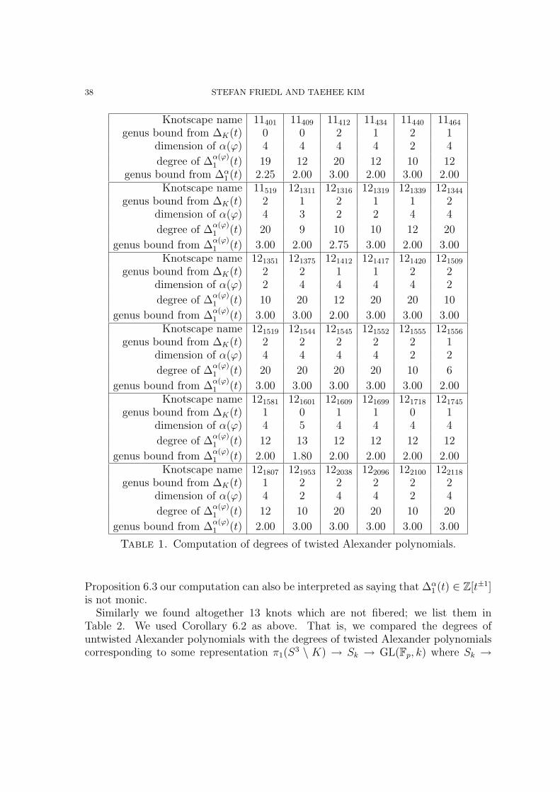
38 STEFAN FRIEDL AND TAEHEE KIM
Knotscape name 11401 11409 11412 11434 11440 11464
genus bound from ∆K(t) 0 0 2 1 2 1dimension of α(ϕ) 4 4 4 4 2 4
degree of ∆α(ϕ)1 (t) 19 12 20 12 10 12
genus bound from ∆α1 (t) 2.25 2.00 3.00 2.00 3.00 2.00
Knotscape name 11519 121311 121316 121319 121339 121344
genus bound from ∆K(t) 2 1 2 1 1 2dimension of α(ϕ) 4 3 2 2 4 4
degree of ∆α(ϕ)1 (t) 20 9 10 10 12 20
genus bound from ∆α(ϕ)1 (t) 3.00 2.00 2.75 3.00 2.00 3.00
Knotscape name 121351 121375 121412 121417 121420 121509
genus bound from ∆K(t) 2 2 1 1 2 2dimension of α(ϕ) 2 4 4 4 4 2
degree of ∆α(ϕ)1 (t) 10 20 12 20 20 10
genus bound from ∆α(ϕ)1 (t) 3.00 3.00 2.00 3.00 3.00 3.00
Knotscape name 121519 121544 121545 121552 121555 121556
genus bound from ∆K(t) 2 2 2 2 2 1dimension of α(ϕ) 4 4 4 4 2 2
degree of ∆α(ϕ)1 (t) 20 20 20 20 10 6
genus bound from ∆α(ϕ)1 (t) 3.00 3.00 3.00 3.00 3.00 2.00
Knotscape name 121581 121601 121609 121699 121718 121745
genus bound from ∆K(t) 1 0 1 1 0 1dimension of α(ϕ) 4 5 4 4 4 4
degree of ∆α(ϕ)1 (t) 12 13 12 12 12 12
genus bound from ∆α(ϕ)1 (t) 2.00 1.80 2.00 2.00 2.00 2.00
Knotscape name 121807 121953 122038 122096 122100 122118
genus bound from ∆K(t) 1 2 2 2 2 2dimension of α(ϕ) 4 2 4 4 2 4
degree of ∆α(ϕ)1 (t) 12 10 20 20 10 20
genus bound from ∆α(ϕ)1 (t) 2.00 3.00 3.00 3.00 3.00 3.00
Table 1. Computation of degrees of twisted Alexander polynomials.
Proposition 6.3 our computation can also be interpreted as saying that ∆α1 (t) ∈ Z[t±1]
is not monic.Similarly we found altogether 13 knots which are not fibered; we list them in
Table 2. We used Corollary 6.2 as above. That is, we compared the degrees ofuntwisted Alexander polynomials with the degrees of twisted Alexander polynomialscorresponding to some representation π1(S
3 \ K) → Sk → GL(Fp, k) where Sk →
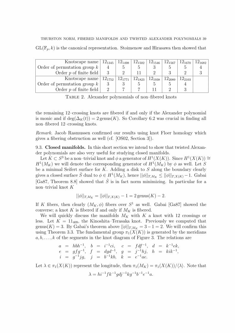
THURSTON NORM, FIBERED MANIFOLDS AND TWISTED ALEXANDER POLYNOMIALS 39
GL(Fp, k) is the canonical representation. Stoimenow and Hirasawa then showed that
Knotscape name 121345 121498 121502 121546 121567 121670 121682
Order of permutation group k 4 5 5 3 5 5 4Order p of finite field 3 2 11 2 3 2 3
Knotscape name 121752 121771 121823 121938 122089 122103
Order of permutation group k 3 3 5 5 5 4Order p of finite field 2 7 7 11 2 3
Table 2. Alexander polynomials of non–fibered knots
the remaining 12–crossing knots are fibered if and only if the Alexander polynomialis monic and if deg(∆K(t)) = 2 genus(K). So Corollary 6.2 was crucial in finding allnon–fibered 12–crossing knots.
Remark. Jacob Rasmussen confirmed our results using knot Floer homology whichgives a fibering obstruction as well (cf. [OS02, Section 3]).
9.3. Closed manifolds. In this short section we intend to show that twisted Alexan-der polynomials are also very useful for studying closed manifolds.
LetK ⊂ S3 be a non–trivial knot and φ a generator ofH1(X(K)). SinceH1(X(K)) ∼=H1(MK) we will denote the corresponding generator of H1(MK) by φ as well. Let Sbe a minimal Seifert surface for K. Adding a disk to S along the boundary clearlygives a closed surface S dual to φ ∈ H1(MK), hence ||φ||T,MK
≤ ||φ||T,X(K)−1. Gabai
[Ga87, Theorem 8.8] showed that S is in fact norm minimizing. In particular for anon–trivial knot K
||φ||T,MK= ||φ||T,X(K) − 1 = 2 genus(K)− 2.
If K fibers, then clearly (MK , φ) fibers over S1 as well. Gabai [Ga87] showed theconverse; a knot K is fibered if and only if MK is fibered.
We will quickly discuss the manifolds MK with K a knot with 12 crossings orless. Let K = 11409, the Kinoshita–Terasaka knot. Previously we computed thatgenus(K) = 3. By Gabai’s theorem above ||φ||T,MK
= 3−1 = 2. We will confirm thisusing Theorem 3.3. The fundamental group π1(X(K)) is generated by the meridiansa, b, . . . , k of the segments in the knot diagram of Figure 3. The relations are
a = hbh−1, b = i−1ci, c = fdf−1, d = k−1ek,e = gfg−1, f = dgd−1, g = j−1hj, h = kik−1,i = g−1jg, j = b−1kb, k = e−1ae.
Let λ ∈ π1(X(K)) represent the longitude, then π1(MK) = π1(X(K))/〈λ〉. Note that
λ = hi−1fk−1gdj−1kg−1b−1e−1a.
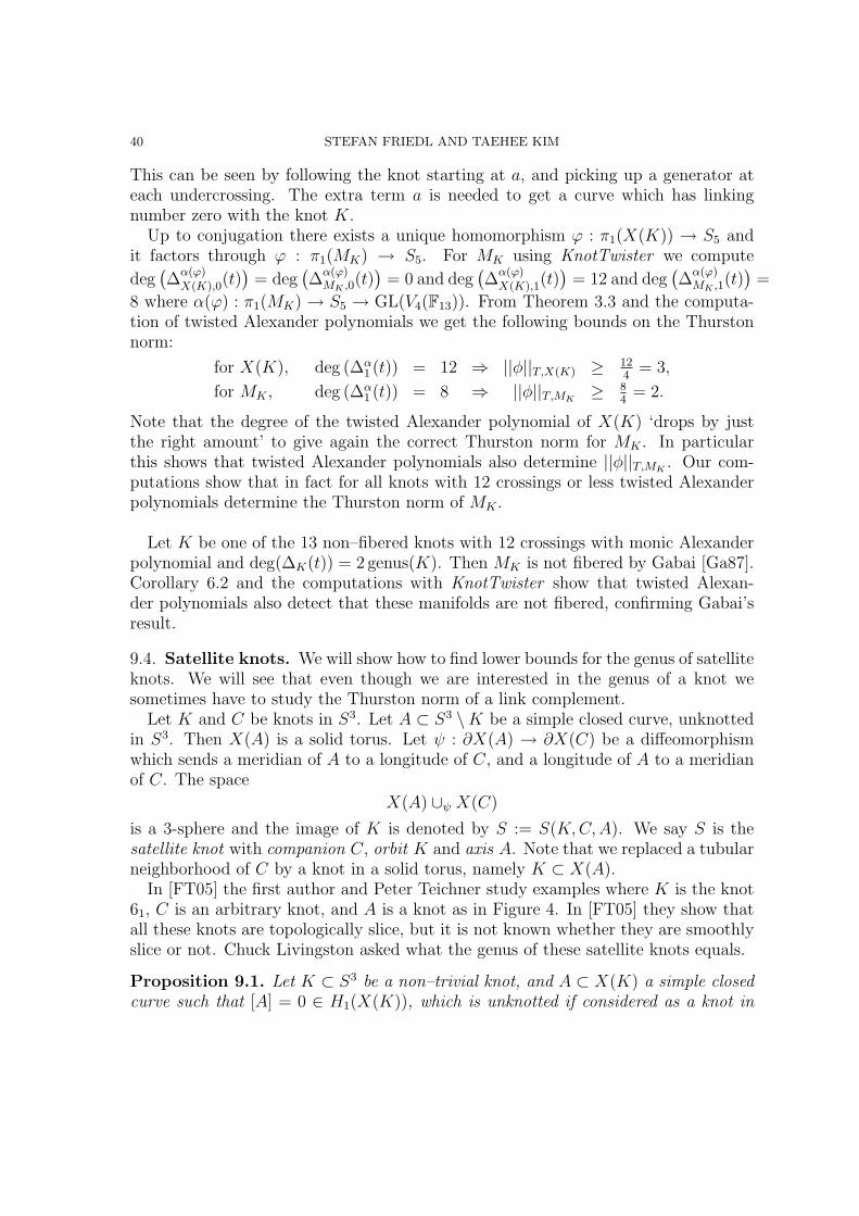
40 STEFAN FRIEDL AND TAEHEE KIM
This can be seen by following the knot starting at a, and picking up a generator ateach undercrossing. The extra term a is needed to get a curve which has linkingnumber zero with the knot K.
Up to conjugation there exists a unique homomorphism ϕ : π1(X(K)) → S5 andit factors through ϕ : π1(MK) → S5. For MK using KnotTwister we compute
deg(∆α(ϕ)X(K),0(t)
)= deg
(∆α(ϕ)MK ,0
(t))
= 0 and deg(∆α(ϕ)X(K),1(t)
)= 12 and deg
(∆α(ϕ)MK ,1
(t))
=
8 where α(ϕ) : π1(MK) → S5 → GL(V4(F13)). From Theorem 3.3 and the computa-tion of twisted Alexander polynomials we get the following bounds on the Thurstonnorm:
for X(K), deg (∆α1 (t)) = 12 ⇒ ||φ||T,X(K) ≥ 12
4= 3,
for MK , deg (∆α1 (t)) = 8 ⇒ ||φ||T,MK
≥ 84
= 2.
Note that the degree of the twisted Alexander polynomial of X(K) ‘drops by justthe right amount’ to give again the correct Thurston norm for MK . In particularthis shows that twisted Alexander polynomials also determine ||φ||T,MK
. Our com-putations show that in fact for all knots with 12 crossings or less twisted Alexanderpolynomials determine the Thurston norm of MK .
Let K be one of the 13 non–fibered knots with 12 crossings with monic Alexanderpolynomial and deg(∆K(t)) = 2 genus(K). Then MK is not fibered by Gabai [Ga87].Corollary 6.2 and the computations with KnotTwister show that twisted Alexan-der polynomials also detect that these manifolds are not fibered, confirming Gabai’sresult.
9.4. Satellite knots. We will show how to find lower bounds for the genus of satelliteknots. We will see that even though we are interested in the genus of a knot wesometimes have to study the Thurston norm of a link complement.
Let K and C be knots in S3. Let A ⊂ S3 \K be a simple closed curve, unknottedin S3. Then X(A) is a solid torus. Let ψ : ∂X(A) → ∂X(C) be a diffeomorphismwhich sends a meridian of A to a longitude of C, and a longitude of A to a meridianof C. The space
X(A) ∪ψ X(C)
is a 3-sphere and the image of K is denoted by S := S(K,C,A). We say S is thesatellite knot with companion C, orbit K and axis A. Note that we replaced a tubularneighborhood of C by a knot in a solid torus, namely K ⊂ X(A).
In [FT05] the first author and Peter Teichner study examples where K is the knot61, C is an arbitrary knot, and A is a knot as in Figure 4. In [FT05] they show thatall these knots are topologically slice, but it is not known whether they are smoothlyslice or not. Chuck Livingston asked what the genus of these satellite knots equals.
Proposition 9.1. Let K ⊂ S3 be a non–trivial knot, and A ⊂ X(K) a simple closedcurve such that [A] = 0 ∈ H1(X(K)), which is unknotted if considered as a knot in
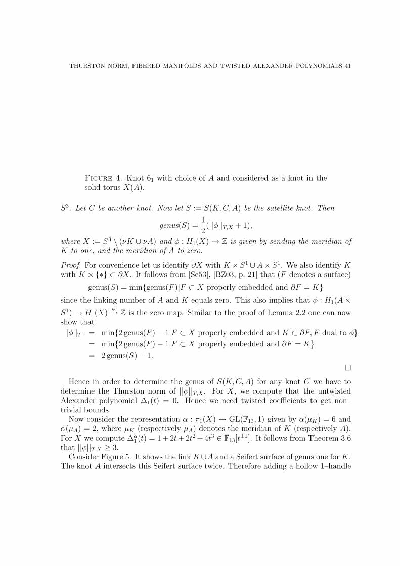
THURSTON NORM, FIBERED MANIFOLDS AND TWISTED ALEXANDER POLYNOMIALS 41
Figure 4. Knot 61 with choice of A and considered as a knot in thesolid torus X(A).
S3. Let C be another knot. Now let S := S(K,C,A) be the satellite knot. Then
genus(S) =1
2(||φ||T,X + 1),
where X := S3 \ (νK ∪ νA) and φ : H1(X) → Z is given by sending the meridian ofK to one, and the meridian of A to zero.
Proof. For convenience let us identify ∂X with K × S1 ∪A× S1. We also identify Kwith K × {∗} ⊂ ∂X. It follows from [Sc53], [BZ03, p. 21] that (F denotes a surface)
genus(S) = min{genus(F )|F ⊂ X properly embedded and ∂F = K}since the linking number of A and K equals zero. This also implies that φ : H1(A×S1) → H1(X)
φ−→ Z is the zero map. Similar to the proof of Lemma 2.2 one can nowshow that
||φ||T = min{2 genus(F )− 1|F ⊂ X properly embedded and K ⊂ ∂F, F dual to φ}= min{2 genus(F )− 1|F ⊂ X properly embedded and ∂F = K}= 2 genus(S)− 1.
�
Hence in order to determine the genus of S(K,C,A) for any knot C we have todetermine the Thurston norm of ||φ||T,X . For X, we compute that the untwistedAlexander polynomial ∆1(t) = 0. Hence we need twisted coefficients to get non–trivial bounds.
Now consider the representation α : π1(X) → GL(F13, 1) given by α(µK) = 6 andα(µA) = 2, where µK (respectively µA) denotes the meridian of K (respectively A).For X we compute ∆α
1 (t) = 1 + 2t+ 2t2 + 4t3 ∈ F13[t±1]. It follows from Theorem 3.6
that ||φ||T,X ≥ 3.Consider Figure 5. It shows the link K∪A and a Seifert surface of genus one for K.
The knot A intersects this Seifert surface twice. Therefore adding a hollow 1–handle
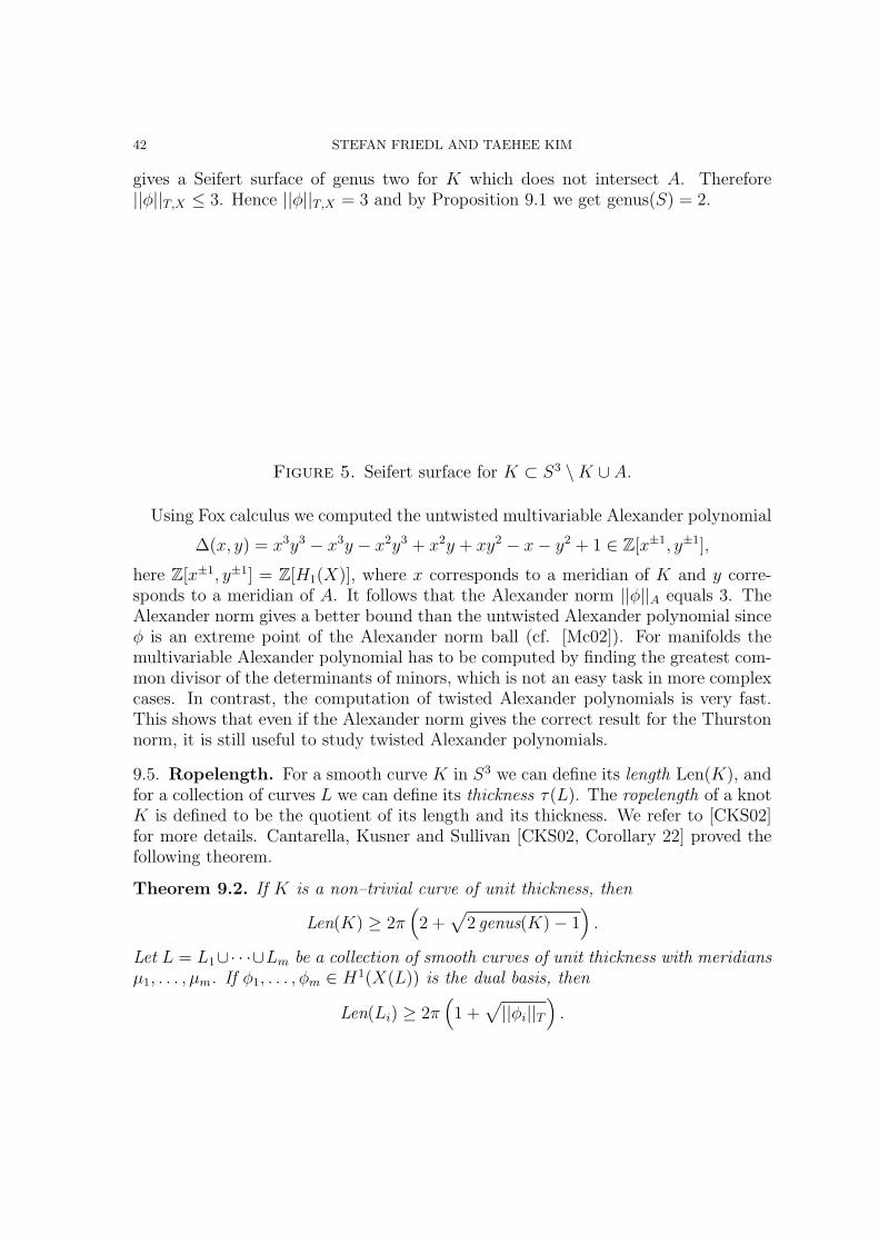
42 STEFAN FRIEDL AND TAEHEE KIM
gives a Seifert surface of genus two for K which does not intersect A. Therefore||φ||T,X ≤ 3. Hence ||φ||T,X = 3 and by Proposition 9.1 we get genus(S) = 2.
Figure 5. Seifert surface for K ⊂ S3 \K ∪ A.
Using Fox calculus we computed the untwisted multivariable Alexander polynomial
∆(x, y) = x3y3 − x3y − x2y3 + x2y + xy2 − x− y2 + 1 ∈ Z[x±1, y±1],
here Z[x±1, y±1] = Z[H1(X)], where x corresponds to a meridian of K and y corre-sponds to a meridian of A. It follows that the Alexander norm ||φ||A equals 3. TheAlexander norm gives a better bound than the untwisted Alexander polynomial sinceφ is an extreme point of the Alexander norm ball (cf. [Mc02]). For manifolds themultivariable Alexander polynomial has to be computed by finding the greatest com-mon divisor of the determinants of minors, which is not an easy task in more complexcases. In contrast, the computation of twisted Alexander polynomials is very fast.This shows that even if the Alexander norm gives the correct result for the Thurstonnorm, it is still useful to study twisted Alexander polynomials.
9.5. Ropelength. For a smooth curve K in S3 we can define its length Len(K), andfor a collection of curves L we can define its thickness τ(L). The ropelength of a knotK is defined to be the quotient of its length and its thickness. We refer to [CKS02]for more details. Cantarella, Kusner and Sullivan [CKS02, Corollary 22] proved thefollowing theorem.
Theorem 9.2. If K is a non–trivial curve of unit thickness, then
Len(K) ≥ 2π(2 +
√2 genus(K)− 1
).
Let L = L1∪· · ·∪Lm be a collection of smooth curves of unit thickness with meridiansµ1, . . . , µm. If φ1, . . . , φm ∈ H1(X(L)) is the dual basis, then
Len(Li) ≥ 2π(1 +
√||φi||T
).
THURSTON NORM, FIBERED MANIFOLDS AND TWISTED ALEXANDER POLYNOMIALS 43
Clearly our methods now give lower bounds on the length of a component of acollection of curves of unit thickness. In [CKS02] the authors consider the link inFigure 6. Denote the component represented by a circle by L1, and the other com-
Figure 6
ponent by L2. Denote the meridian of Li by µi for i = 1, 2. Attach a half–sphereto L1 ‘below the paper plane’. Removing three disks and adding star shaped ‘pants’gives a Seifert surface for L1 of genus two which does not intersect L2. In [CKS02]the authors conjectured that the above surface is minimal, i.e., that ||φ1||T = 3 forφ1 the homomorphism with φ1(µ1) = 1, φ1(µ2) = 0. Harvey [Ha05, Section 8] usedhigher–order Alexander polynomials to prove the conjecture in the positive. We willreprove this using twisted Alexander polynomials.
Consider the representation α : π1(X(L)) → GL(F13, 1) given by α(µ1) = 10 andα(µ2) = 7. Then ∆α
1 (t) = 1 + 4t2 + 2t3 ∈ F13[t±1]. It follows from Theorem 5.1 that
||φ||T ≥ 31− 1 = 2. By Lemma 3.4 ||φ||T ≡ 10 + 7 mod 2, hence it is odd. Therefore
||φ||T ≥ 3, which reproves the conjecture of [CKS02]. In particular it follows that theropelength of L1 is at least 2π(1 +
√3). Using similar arguments, one can show that
the ropelength of L2 is also at least 2π(1 +√
3).
9.6. 9–crossing links. McMullen [Mc02] determined the Thurston norm for all linkswith 9 or fewer crossings and with three or fewer components, except for 93
21, 9241, 9
250
and 9315 (here we use Rolfsen’s [Rol90] notation). For the link 93
21 the multivari-able Alexander polynomial vanishes, and also all twisted Alexander polynomials wecomputed vanish.
In the case of the other three links McMullen computed the Alexander norm, butcould not show that it agrees with the Thurston norm for all φ. We computed twistedAlexander polynomials for the extreme points of the Alexander norm ball for the links92
41 and 9250 and our computations strongly suggest that the Alexander norm agrees
with the Thurston norm in these two cases.
9.7. Dunfield’s link. We will show that our invariants also detect subtle examplesof pairs (X(L), φ) where L is a link in S3 and φ ∈ H1(X(L)), which do not fiber overS1. Consider the link L in Figure 7 from [Du01]. Denote the knotted componentby L1 and the unknotted component by L2. Let x, y ∈ H1(X(L)) be the elements
44 STEFAN FRIEDL AND TAEHEE KIM
Figure 7. Dunfield’s link.
represented by a meridian of L1 respectively L2. Then the multivariable Alexanderpolynomial equals
∆X(L) = xy − x− y + 1 ∈ Z[H1(X(L))] = Z[x±1, y±1].
The Alexander norm ball (cf. [Mc02] for a definition) and the Thurston norm ball(which is determined in [FK05]) are given in Figure 8. Dunfield [Du01] showed that
Figure 8. Alexander norm ball and Thurston norm ball for Dunfield’s link.
(X(L), φ) fibers over S1 for all φ ∈ H1(M) in the cone on the two open faces withvertices (−1
2, 1
2), (0, 1) respectively (0,−1), (1
2,−1
2). He also showed that (X(L), φ)
does not fiber over S1 for any φ ∈ H1(X(L)) lying outside the cone. Later in [FK05]the authors completely determined the Thurston norm of X(L).
Now let φ be the homomorphism given by φ(x) = 1, φ(y) = −1. In that case φ isinside the cone on an open face of the Alexander norm ball and ∆1(t) = 1−3t+3t2−t3 ∈ Z[t±1] is monic. Hence the abelian invariants are inconclusive whether (X(L), φ)is fibered or not. On the other hand we found a representation π1(X(L)) → S3 →GL(F2, 3) such that ∆α
1 (t) = 0 ∈ F2[t±1]. Therefore (X(L), φ) does not fiber over
S1 by Theorem 6.1. Note that the fact that (X(L), φ) does not fiber over S1 alsofollows from the fact that φ is not in the cone on a top–dimensional open face of theThurston norm ball (cf. [Th86] and [Oe86]).
10. Conjectures
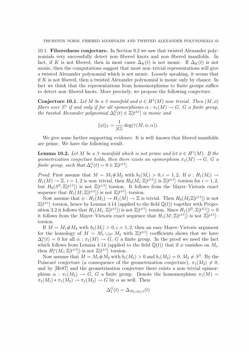
THURSTON NORM, FIBERED MANIFOLDS AND TWISTED ALEXANDER POLYNOMIALS 45
10.1. Fiberedness conjecture. In Section 9.2 we saw that twisted Alexander poly-nomials very successfully detect non–fibered knots and non–fibered manifolds. Infact, if K is not fibered, then in most cases ∆K(t) is not monic. If ∆K(t) is notmonic, then the computations suggest that most non–trivial representations will givea twisted Alexander polynomial which is not monic. Loosely speaking, it seems thatif K is not fibered, then a twisted Alexander polynomial is monic only by chance. Infact we think that the representations from homomorphisms to finite groups sufficeto detect non–fibered knots. More precisely, we propose the following conjecture.
Conjecture 10.1. Let M be a 3–manifold and φ ∈ H1(M) non–trivial. Then (M,φ)fibers over S1 if and only if for all epimorphisms α : π1(M) → G, G a finite group,the twisted Alexander polynomial ∆G
1 (t) ∈ Z[t±1] is monic and
||φ||T =1
|G|deg(τ(M,φ, α)).
We give some further supporting evidence. It is well–known that fibered manifoldsare prime. We have the following result.
Lemma 10.2. Let M be a 3–manifold which is not prime and let φ ∈ H1(M). If thegeometrization conjecture holds, then there exists an epimorphism π1(M) → G, G afinite group, such that ∆G
1 (t) = 0 ∈ Z[t±1].
Proof. First assume that M = M1#M2 with b1(Mi) > 0, i = 1, 2. If φ : H1(Mi) →H1(M) → Z, i = 1, 2 is non–trivial, then H0(Mi; Z[t±1]) is Z[t±1]–torsion for i = 1, 2,but H0(S
2; Z[t±1]) is not Z[t±1] torsion. It follows from the Mayer–Vietoris exactsequence that H1(M ; Z[t±1]) is not Z[t±1]–torsion.
Now assume that φ : H1(M1) → H1(M) → Z is trivial. Then H0(M1Z[t±1]) is notZ[t±1]–torsion, hence by Lemma 4.14 (applied to the field Q(t)) together with Propo-sition 3.2 it follows that H1(M1; Z[t±1]) is not Z[t±1]–torsion. Since H1(S
2; Z[t±1]) = 0it follows from the Mayer–Vietoris exact sequence that H1(M ; Z[t±1]) is not Z[t±1]–torsion.
If M = M1#M2 with b1(Mi) > 0, i = 1, 2, then an easy Mayer–Vietoris argumentfor the homology of M = M1 ∪S2 M2 with Z[t±1]–coefficients shows that we have∆α
1 (t) = 0 for all α : π1(M) → G, G a finite group. In the proof we need the factwhich follows from Lemma 4.14 (applied to the field Q(t)) that if φ vanishes on Mi,then Hα
1 (Mi; Z[t±1]) is not Z[t±1]–torsion.Now assume that M = M1#M2 with b1(M1) > 0 and b1(M2) = 0, M2 6= S3. By the
Poincare conjecture (a consequence of the geometrization conjecture), π1(M2) 6= 0,and by [He87] and the geometrization conjecture there exists a non–trivial epimor-phism α : π1(M2) → G, G a finite group. Denote the homomorphism π1(M) =π1(M1) ∗ π1(M2) → π1(M2) → G by α as well. Then
∆G1 (t) = ∆MG,φG,1(t)
46 STEFAN FRIEDL AND TAEHEE KIM
by Lemma 3.8 where MG is the cover of M corresponding to M . But the primedecomposition of MG has |G| copies of M1, in particular by the above observationthat ∆M,φ,1(t) = ∆MG,φG,1(t) = 0. �
Proposition 10.3. Let S = S(K,C,A) be a satellite knot with A ∈ π1(S3 \ K)(1)
and ∆C(t) 6= 1. Then there exists a homomorphism α : π1(S) → G, G a finite group,such that ∆G
X(S),1(t) is not monic.
Note that combining this proposition with Theorem 6.1 we come close to reprovingthe more general fact that if K and C are any knots and A ∈ π1(S
3 \K)(1) then S isnot fibered, which follows from studying π1(S
3 \ S)(1) (cf. [BZ03, p. 64]).
Proof. First let α : π1(X(K)) → G be any homomorphism to a finite group. Denotethe order of α(A) ∈ G by r and write LC,r for the r–fold cover of S3 branched alongC. By [Ch03, Section 4] there exists a surjective map π1(X(S)) → π1(X(K)) suchthat ∆G
X(S),1(t) ∈ Z[t±1] is an annihilator for H1(LC,r)⊗Z Z[t±1].
Clearly we are done, once we can arrange α such that H1(LC,r) is either infinite ornon–trivial torsion. By Riley [Ri90] the finite values |H1(LC,r)| grow exponentially inr, in particular there exists R ∈ N such that H1(LC,r) is either infinite or non–trivialtorsion for all r ≥ R.
Since π1(X(K)) is residually finite (cf. [Th82, He87]) an easy argument shows thatwe can find an epimorphism α : π1(X(K)) → G, G finite, such that α(Ak) 6= e forany k < R. In particular the order of α(A) in G is bigger than or equal to R. �
We explain a possible approach to Conjecture 10.1. Let M be a 3–manifold whoseboundary is empty or consists of tori and φ ∈ H1(M) non–trivial. Assume thatfor every representation α : π1(M) → G, G a finite group, the twisted Alexanderpolynomial ∆G
1 (t) is monic and
||φ||T =1
|G|deg(τ(M,φ, α)).
Assuming the geometrization conjecture we get from Lemma 10.2 that M is prime.Let S be a surface dual to φ with minimal complexity. Clearly Hα
0 (M ; Z[G][t±1]) 6=0 , hence ∆G
0 (t) 6= 1. Combining this observation with the fact that ∆G1 (t) 6= 0 (which
is obvious from the assumption), we can assume by Corollary 4.8 that S is connected.Then let N be the result of cutting M along S. Denote the positive and the negativeinclusions of S into N by i+ and i−. Since S is minimal, i+ : π1(S) → π1(N) isinjective by Dehn’s Lemma. Since M is prime it follows easily from Stallings’ theorem[St62] that (M,φ) fibers over S1 if and only if i+ : π1(S) → π1(N) is surjective (cf.also [Ka96, p. 84] in the knot complement case).
Proposition 10.4. Hα1 (S; Z[G]) and Hα
1 (N ; Z[G]) are free abelian groups of the samerank.
THURSTON NORM, FIBERED MANIFOLDS AND TWISTED ALEXANDER POLYNOMIALS 47
Proof. First note that Hα1 (S; Z[G]) is the first homology of the cover of S correspond-
ing to π1(S) → G, hence Hα1 (S; Z[G]) is free abelian.
Let p be a prime. It follows from the proof of Proposition 6.3 that ∆αp
1 (t) 6= 0 forthe representation αp : π1(M) → G → GL(Fp, |G|). In particular . By Lemma 4.2Hα
2 (M ; Fp[G][t±1]) is Fp[t±1]–torsion. Therefore we have a short exact sequence
0 → Hαp
1 (S; Fp[G])⊗FpFp[t±1] → Hαp
1 (N ; Fp[G])⊗FpFp[t±1] → Hαp
1 (M ; Fp[G][t±1]) → 0.
In particular Hαp
1 (S; Fp[G]) ∼= Hαp
1 (N ; Fp[G]) for every prime p as Fp–vector spaces.Note thatHα
0 (S; Z[G]) ∼= Z[G/Im{π1(S) → G}] andHα0 (N ; Z[G]) ∼= Z[G/Im{π1(N) →
G}] in particular both are Z–torsion free. It follows from the universal coefficient the-orem applied to the Z–module complex C∗(S)⊗Z[π1(S)] Z[G] that
Hα1 (S; Z[G])⊗Z Fp ∼= H
αp
1 (S; Fp[G])
for every prime p. The same statement holds for N . Combining our results wesee that Hα
1 (S; Z[G]) ⊗Z Fp ∼= Hα1 (N ; Z[G]) ⊗Z Fp for any prime p. It follows that
Hα1 (S; Z[G]) ∼= Hα
1 (N ; Z[G]).�
Now consider the exact sequence
Hα1 (S; Z[G])⊗ Z[t±1]
ti+−i−−−−−→ Hα1 (N ; Z[G])⊗ Z[t±1] → Hα
1 (M ; Z[G][t±1]) → 0.
Since Hα1 (S; Z[G]) and Hα
1 (N ; Z[G]) are free abelian groups of the same rank it followsthat ∆G
1 (t) = det(ti+ − i−) (we refer to [Ch03] for the definition of ∆G1 (t) ∈ Z[t±1]).
Using Lemmas 4.7, 4.9 and 4.14 we see that the assumption
||φ||T =1
|G|(deg
(∆G
1 (t))− deg
(∆G
0 (t))− deg
(∆G
2 (t)) )
implies that deg(det(ti+ − i−)) = deg(∆G
1 (t))
= rank(Hα1 (S; Z[G])). In particular
det(i+) 6= 0 and det(i−) 6= 0. The assumption that the twisted Alexander polynomial∆G
1 (t) is monic implies that in fact det(i+) = ±1 and det(i−) = ±1. Thereforethe question is whether i+ : π1(S) → π1(N) is surjective if i+ : Hα
1 (S; Z[G]) →Hα
1 (N ; Z[G]) is surjective for every representation π1(M) → G, G a finite group.This discussion shows that Conjecture 10.1 follows from the geometrization con-
jecture and the following group–theoretic question.
Conjecture 10.5. Let S be an incompressible surface in a 3–manifold M and let Nbe M cut along S. Let i : S → N be one of the positive and the negative inclusions ofS into N . If i : Hα
1 (S; Z[G]) → Hα1 (N ; Z[G]) is surjective for every homomorphism
π1(M) → G, G a finite group, then i : π1(S) → π1(N) is surjective.
Note that it is well–known that the inclusion induced homomorphisms π1(S) →π1(M) and π1(N) → π1(M) are injections. We think that an affirmative answer to theabove conjecture will need a strong condition on π1(M) (of which π1(N) and π1(S) aresubgroups) such as subgroup separability, which is conjectured to hold for fundamental
48 STEFAN FRIEDL AND TAEHEE KIM
groups of hyperbolic manifolds (cf. [Th82]) but does not hold for fundamental groupsin general (cf. [NW01]). On the other hand, knots which are not hyperbolic areeither torus knots (and therefore fibered), or satellite knots, which can perhaps bedealt with differently, as in Proposition 10.3.
10.2. Knot genus conjecture. As we pointed out in Section 5 there exist manymanifolds such that ∆α
1 (t) = 0 for all φ ∈ H1(M) and all representations α. Eventhough Theorem 5.1 can still give some partial information, it is clear that in thecase b1(M) > 1 in general we can not expect to get the Thurston norm from twistedAlexander polynomials. As we pointed out in Section 5, we can not even determinewhether a surface with minimal complexity dual to some φ ∈ H1(M) is connected ornot.
It follows immediately from the definition of twisted Alexander polynomials that∆α
1 (t) is determined by the fundamental group ofM . Therefore it is a natural questionwhether the Thurston norm is determined by the fundamental group. Note that theThurston norm of a manifold is determined by its prime components. If M is aprime manifold with H1(M) 6= 0, then M is Haken and by Waldhausen’s work it isdetermined by its peripheral system. In particular if M is closed and Haken, then itis determined by its fundamental group.
In the case of a knot complement X(K) Feustel and Whitten [FW78, Corollary 3]showed that the genus of a knot K is determined by π1(X(K)). We do not knowwhether π1(M) determines the Thurston norm for every manifolds with boundary.
We conjecture that twisted Alexander polynomials determine the genus of hyper-bolic knots. More precisely we formulate the following conjecture.
Conjecture 10.6. Let K ⊂ S3 be a hyperbolic knot and φ ∈ H1(X(K)) a generator.Then there exists an epimorphism α : π1(M) → G such that
1
|G|(deg
(∆G
1 (t))− deg
(∆G
0 (t)) )
> ||φ||T − 1.
It turns out that this question is similar in nature to Conjecture 10.1. Indeed, letS be a minimal Seifert surface for K. Then the maps
i+, i− : π1(S) → π1(S3 \ νS)
are injective. The goal now is to show that there exists a map π1(X(K)) → G suchthat the induced maps on homology
i+, i− : Hα1 (S; Z[G]) → Hα
1 (S3 \ νS; Z[G])
are ‘almost’ injective. For example if Hα1 (S; Z[G]) and Hα
1 (S3 \ νS; Z[G]) are isomor-phic as Z–modules and i+, i− are isomorphisms, then ∆G
1 (t) has degree rankZ(Hα1 (S; Z[G]))
and therefore
||φ||T =1
|G|(deg
(∆G
1 (t))− deg
(∆G
0 (t)) ).
THURSTON NORM, FIBERED MANIFOLDS AND TWISTED ALEXANDER POLYNOMIALS 49
Hence again we have to detect a property of the map on the fundamental group levelin a map of appropriate homology groups.
Remark. Let K1 and K2 be knots and assume there exists an epimorphism ϕ :π1(X(K1)) → π1(X(K2)). Simon asked (cf. question 1.12 (b) on Kirby’s problem list[Kir97]) whether this implies that genus(K1) ≥ genus(K2). Let α : π1(X(K2)) → Gbe an epimorphism to a finite group. By [KSW04] ∆α
K2(t) divides ∆α◦ϕ
K1(t). Thus
our results strongly suggest an affirmative answer to Simon’s question, and clearly apositive solution to our conjecture would answer Simon’s question.
References
[BZ03] G. Burde and H. Zieschang, Knots, second edition, de Gruyter Studies in Mathematics, 5.Walter de Gruyter & Co. , Berlin, 2003.
[CKS02] J. Cantarella, R. B. Kusner and J. M. Sullivan, On the Minimum Ropelength of Knots andLinks, Invent. Math. 150 (2002), no. 2, 257–286.
[Ch03] J. Cha, Fibred knots and twisted Alexander invariants, Trans. Amer. Math. Soc. 355 (2003),no. 10, 4187–4200 (electronic).
[Co04] T. Cochran, Noncommutative knot theory, Algebr. Geom. Topol. 4 (2004), 347–398.[CK02] J.C. Crager and P. R. Kotiuga, cuts for the magnetic scalar potential in knotted geometrics
and force–free magnetic fields, IEEE Trans. Magn. vol 38, (2002) 1309–1311[Cr59] R. H. Crowell, Genus of alternating link types, Ann. of Math. (2) 69 1959 258–275.[CF77] R. Crowell and R. Fox, Introduction to knot theory, reprint of the 1963 original. Graduate
Texts in Mathematics, No. 57. Springer-Verlag, New York-Heidelberg, 1977.[Du01] N. Dunfield, Alexander and Thurston norms of fibered 3–manifolds, Pacific J. Math. 200
(2001), no. 1, 43–58.[FW78] C. D. Feustel and W. Whitten, Groups and complements of knots, Canad. J. Math. 30
(1978), no. 6, 1284–1295.[FS98] R. Fintushel and R. Stern, Knots, links, and 4-manifolds, Invent. Math. 134 (1998), no. 2,
363–400.[Fo53] R. H. Fox, Free differential calculus I, derivation in the free group ring, Ann. of Math. (2)
57, (1953). 547–560.[Fo54] R. H. Fox, Free differential calculus II, the isomorphism problem, Ann. of Math. (2) 59,
(1954). 196–210.[FH91] M. H. Freedman and Z. He, Divergence–free fields: Energy and asymptotic crossing number,
Ann. of Math. (2) 134 (1991), no. 1, 189–229.[F05] S. Friedl, KnotTwister, http://math.rice.edu/~ friedl/index.html (2005).[F05b] S. Friedl, Reidemeister torsion, the Thurston norm and Harvey’s invariants, preprint (2005)[FK05] S. Friedl and T. Kim, Twisted Alexander norms give lower bounds on the Thurston norm,
preprint (2005).[FT05] S. Friedl ad P. Teichner, New topologically slice knots, Preprint (2005)[FV05] S. Friedl and S. Vidussi, Twisted Alexander polynomials and symplectic structures, in prepa-
ration (2005)[Ga83] D. Gabai, Foliations and the topology of 3–manifolds, J. Differential Geom. 18 (1983), no.
3, 445–503.[Ga84] D. Gabai, Foliations and genera of links, Topology 23 (1984), no. 4, 381–394.[Ga87] D. Gabai, Foliations and the topology of 3–manifolds. III, J. Differential Geom. 26 (1987),
no. 3, 479–536.
50 STEFAN FRIEDL AND TAEHEE KIM
[GKM05] H. Goda, T. Kitano and T. Morifuji, Reidemeister torsion, twisted Alexander polynomialsand fibered knots, Comment. Math. Helv. 80 (2005), no. 1, 51–61.
[Ha05] S. Harvey, Higher–order polynomial invariants of 3–manifolds giving lower bounds for theThurston norm, Topology 44: 895–945 (2005)
[Ha06] S. Harvey, Monotonicity of degrees of generalized Alexander polynomials of groups and 3–manifolds, preprint arXiv:math. GT/0501190, to appear in Math. Proc. Camb. Phil. Soc. (2006)
[He87] J. Hempel, Residual finiteness for 3-manifolds, Combinatorial group theory and topology(Alta, Utah, 1984), 379–396, Ann. of Math. Stud., 111, Princeton Univ. Press, Princeton, NJ,1987.
[Hi02] J. Hillman, Algebraic invariants of links, Series on Knots and Everything, 32. World ScientificPublishing Co., Inc., River Edge, NJ, 2002.
[HLN04] J. A. Hillman, C. Livingston and S. Naik, Twisted Alexander polynomials of periodic knots,preprint (2004) arXiv:math. GT/0412380.
[HT] J. Hoste and M. Thistlethwaite, Knotscape, http://www.math.utk.edu/~morwen/knotscape.html
[JW93] B. Jiang and S. Wang, Twisted topological invariants associated with representations, Topicsin knot theory (Erzurum, 1992), 211–227, NATO Adv. Sci. Inst. Ser. C Math. Phys. Sci., 399,Kluwer Acad. Publ., Dordrecht, 1993.
[Ka96] A. Kawauchi, A survey of knot theory, translated and revised from the 1990 Japanese originalby the author. Birkhauser Verlag, Basel, 1996.
[Kir97] R. Kirby, Problems in low–dimensional topology, edited by Rob Kirby. AMS/IP Stud. Adv.Math., 2.2, Geometric topology (Athens, GA, 1993), 35–473, Amer. Math. Soc., Providence,RI, 1997.
[KL99a] P. Kirk and C. Livingston, Twisted Alexander invariants, Reidemeister torsion and Casson–Gordon invariants, Topology 38 (1999), no. 3, 635–661.
[KL99b] P. Kirk and C. Livingston, Twisted knot polynomials: inversion, mutation and concordan,Topology 38 (1999), no. 3, 663–671.
[Kit96] T. Kitano, Twisted Alexander polynomials and Reidemeister torsion, Pacific J. Math. 174(1996), no. 2, 431–442.
[KSW04] T. Kitano, M. Suzuki and M. Wada, Twisted Alexander polynomial and surjectivity of agroup homomorphism, University of Tokyo, Mathematical Sciences Publication 2004–36 (2004).
[Ko04] P. R. Kotiuga, Topology–based inequalities and inverse problems for near force–free magneticfields, IEEE Trans. Magn. 40, no. 2: 1108–1111 (2004)
[Kr98] P. Kronheimer, Embedded surfaces and gauge theory in three and four dimensions, Surveys indifferential geometry, Vol. III (Cambridge, MA, 1996), 243–298, Int. Press, Boston, MA, 1998.
[Kr99] P. Kronheimer, Minimal genus in S1 ×M3, Invent. Math. 135 (1999), no. 1, 45–61.[KM97] P. Kronheimer and T. Mrowka, Scalar curvature and the Thurston norm, Math. Res. Lett.
4 (1997), no. 6, 931–937.[Lic97] W. B. R. Lickorish, An introduction to knot theory, Graduate Texts in Mathematics, 175.
Springer-Verlag, New York, 1997.[Lin01] X. S. Lin, Representations of knot groups and twisted Alexander polynomials, Acta Math.
Sin. (Engl. Ser.) 17 (2001), no. 3, 361–380.[Mc02] C. T. McMullen, The Alexander polynomial of a 3–manifold and the Thurston norm on
cohomology, Ann. Sci. Ecole Norm. Sup. (4) 35 (2002), no. 2, 153–171.[Mu58a] K. Murasugi, On the genus of the alternating knot I, J. Math. Soc. Japan 10 1958 94–105.[Mu58b] K. Murasugi, On the genus of the alternating knot II, J. Math. Soc. Japan 10 1958 9235–
248.
THURSTON NORM, FIBERED MANIFOLDS AND TWISTED ALEXANDER POLYNOMIALS 51
[NW01] G. Niblo and D. Wise, Subgroup separability, knot groups and graph manifolds, Proc. Amer.Math. Soc. 129 (2001), no. 3, 685–693.
[Oe86] U. Oertel, Homology branched surfaces: Thurston’s norm on H2(M3), Low-dimensionaltopology and Kleinian groups (Coventry/Durham, 1984), 253–272, London Math. Soc. Lec-ture Note Ser., 112, Cambridge Univ. Press, Cambridge, 1986.
[OS02] P. Ozsvath and Z. Szabo, Heegaard Floer homologies and contact structures, preprint (2002)arXiv:math. SG/0210127.
[OS04a] P. Ozsvath and Z. Szabo, Holomorphic disks and genus bounds, Geom. Topol. 8 (2004),311–334 (electronic).
[OS04b] P. Ozsvath and Z. Szabo, Knot Floer homology, genus bounds, and mutation, TopologyAppl. 141 (2004), no. 1-3, 59–85.
[Pa04] A. Pajitnov, Novikov homology, Twisted Alexander polynomials and Thurston cones, preprint(2004)
[Ri90] R. Riley, Growth of order of homology of cyclic branched covers of knots, Bull. London Math.Soc. 22 (1990), no. 3, 287–297.
[Rol90] D. Rolfsen, Knots and links, Mathematics Lecture Series, No. 7. Publish or Perish, Inc.,Berkeley, Calif., 1976.
[Sc53] H. Schubert, Knoten und Vollringe, Acta Math. 90 (1953), 131–286.[St62] J. Stallings, On fibering certain 3–manifolds, 1962 Topology of 3–manifolds and related topics
(Proc. The Univ. of Georgia Institute, 1961) pp. 95–100 Prentice-Hall, Englewood Cliffs, N.J.[Sto] A. Stoimenow, http://www.ms.u-tokyo.ac.jp/~ stoimeno/ptab/index.html[Ta94] C. Taubes, The Seiberg–Witten invariants and symplectic forms, Math. Res. Lett. 1 (1994),
809–822.[Ta95] C. Taubes, More constraints on symplectic forms from Seiberg–Witten invariants, Math. Res.
Lett., 2, (1995), 9–13.[Th82] W. P. Thurston, Three dimensional manifolds, Kleinian groups and hyperbolic geometry,
Bull. Amer. Math. Soc. (N.S.) 6 (1982), no. 3, 357–381.[Th86] W. P. Thurston, A norm for the homology of 3–manifolds, Mem. Amer. Math. Soc. 59 (1986),
no. 339, i–vi and 99–130.[Tu01] V. Turaev, Introduction to Combinatorial Torsions, Lectures in Mathematics, ETH Zurich
(2001)[Tu02a] V. Turaev, Torsions of 3–manifolds, Progress in Mathematics, 208. Birkhauser Verlag,
Basel, 2002.[Tu02b] V. Turaev, A homological estimate for the Thurston norm, preprint (2002),
arXiv:math. GT/0207267[Vi99] S. Vidussi, The Alexander norm is smaller than the Thurston norm; a Seiberg–Witten proof,
Prepublication Ecole Polytechnique 6 (1999).[Vi03] S. Vidussi, Norms on the cohomology of a 3–manifold and SW theory, Pacific J. Math. 208
(2003), no. 1, 169–186.[Wa94] M. Wada, Twisted Alexander polynomial for finitely presentable groups, Topology 33 (1994),
no. 2, 241–256.
Rice University, Houston, Texas, 77005-1892E-mail address: [email protected], [email protected]