the three-dimensional spatial autocorrelation of...

The three-dimensional spatial autocorrelation of ionospherically propagated wave packets at high latitudes

Ryan Riddolls Defence R&D – Ottawa

.

Defence R&D Canada – Ottawa Technical Memorandum

DRDC Ottawa TM 2012-158 December 2012

The three-dimensional spatial autocorrelationof ionospherically propagated wave packetsat high latitudesRyan J. RiddollsDefence R&D Canada – Ottawa

Defence R&D Canada – OttawaTechnical MemorandumDRDC Ottawa TM 2012-158December 2012

Principal Author

Original signed by R. J. Riddolls

R. J. Riddolls

Approved by

Original signed by A. Damini

A. DaminiActing Head/Radar Systems Section

Approved for release by

Original signed by C. McMillan

C. McMillanHead/Document Review Panel

c© Her Majesty the Queen in Right of Canada as represented by the Minister ofNational Defence, 2012

c© Sa Majeste la Reine (en droit du Canada), telle que representee par le ministrede la Defense nationale, 2012

Abstract

We analytically derive a three-dimensional spatial autocorrelation function for thephase of ionospherically propagated wave packets at near-vertical magnetic field dipangles. The correlation length in the direction normal to the plane of propagationis approximately equal to the outer scale size of plasma irregularities in the iono-sphere. The correlation length in the horizontal direction in the plane of propagationis approximately equal to one-half the horizontal length of the ionospheric path tran-sited by the wave packet. The vertical correlation length is shown to be equal to thehorizontal correlation length multiplied by the tangent of the wave packet take-offangle.

Resume

Nous developpons analytiquement une fonction d’autocorrelation tridimensionnellepour la phase de paquets d’ondes a propagation ionospherique a des angles d’incli-naison du champ magnetique presque verticaux. La longueur de correlation dans ladirection normale au plan de propagation est environ egale a la taille des plus grandesirregularites plasmatiques de l’ionosphere. La longueur de correlation dans la direc-tion horizontale du plan de propagation est environ egale a la moitie de la longueurhorizontale du trajet ionospherique suivi par le paquet d’ondes. On montre que lalongueur verticale de correlation est egale a la longueur de correlation horizontalemultipliee par la tangente de l’angle de rayonnement du paquet d’ondes.

DRDC Ottawa TM 2012-158 i

This page intentionally left blank.

ii DRDC Ottawa TM 2012-158

Executive summary

The three-dimensional spatial autocorrelation ofionospherically propagated wave packets at highlatitudes

Ryan J. Riddolls; DRDC Ottawa TM 2012-158; Defence R&D Canada – Ottawa;December 2012.

Background: Correlation functions describe the degree to which measured quanti-ties are consistent from one measurement to the next. In the case of measurementsof the same quantity at different points in space, one speaks of the spatial auto-correlation function. Directional radio systems operate on the assumption of goodcorrelation of the phase of an electric field at different points in space. The spatialautocorrelation of an electric field associated with an electromagnetic wave packet ismodified by propagation through the ionosphere. This report theoretically derives asimple spatial autocorrelation function for ionospherically propagated wave packets.

Results: An analytic formula is derived based on a linear plasma density profile forthe ionosphere and a power-law turbulence spectrum for ionospheric irregularities.The correlation length in the direction normal to the plane of propagation is approx-imately equal to the outer scale size of plasma irregularities in the ionosphere. Thecorrelation length in the horizontal direction in the plane of propagation is approxi-mately equal to one-half the horizontal length of the ionospheric path transited by thewave packet. The vertical correlation length is shown to be equal to the horizontalcorrelation length multiplied by the tangent of the wave packet take-off angle.

Significance: This work provides guidance for interpreting the results of radio ex-periments and for proposing future radio systems. In particular, autocorrelationfunctions provide insight on the degree to which ionospheric modes at various eleva-tion and azimuth directions of arrival can be separated by analysis of the spatiallydependent phase.

Future Work: It would be beneficial to look at the case of a general magnetic fielddip angle, although it does not seem to be analytically tractable at this time. Thisanalysis would support the interpretation of results obtained at lower latitudes, andillustrate the quality of the approximation of a vertical magnetic field dip angle madein the current work.

DRDC Ottawa TM 2012-158 iii

Sommaire

The three-dimensional spatial autocorrelation ofionospherically propagated wave packets at highlatitudes

Ryan J. Riddolls; DRDC Ottawa TM 2012-158; R & D pour la defense Canada –Ottawa; decembre 2012.

Contexte : Les fonctions de correlation expriment le degre auquel les quantites me-surees sont coherentes d’une mesure a l’autre. Dans le cas de mesures de la memequantite a differents points dans l’espace, on parle de fonction d’autocorrelation spa-tiale. Les systemes radio directifs fonctionnent en presumant qu’il y a une bonnecorrelation de la phase d’un champ electrique a differents points dans l’espace. L’auto-correlation spatiale d’un champ electrique associe a un paquet d’ondes electromagne-tiques est modifiee par la propagation dans l’ionosphere. Le present rapport presentele developpement theorique d’une fonction d’autocorrelation spatiale simple pour lespaquets d’ondes se propageant dans l’ionosphere.

Resultats : Une formule analytique est developpee a partir d’un profil lineaire de den-site de plasma dans l’ionosphere et d’un spectre de turbulence regi par une loi de puis-sance pour les irregularites plasmatiques de l’ionosphere. La longueur de correlationdans la direction normale au plan de propagation est environ egale a la taille desplus grandes irregularites plasmatiques de l’ionosphere. La longueur de correlationdans la direction horizontale du plan de propagation est environ egale a la moitiede la longueur horizontale du trajet ionospherique suivi par le paquet d’ondes. Onmontre que la longueur verticale de correlation est egale a la longueur de correlationhorizontale multipliee par la tangente de l’angle de rayonnement du paquet d’ondes.

Portee : Ces travaux fournissent des connaissances utiles a l’interpretation desresultats d’experiences radio et a l’etablissement de propositions pour de futurs sys-temes radio. En particulier, les fonctions d’autocorrelation donnent une idee du degreauquel les modes ionospheriques a diverses directions d’arrivee en azimut et en sitepeuvent etre separes par analyse des variations de la phase dans l’espace.

Recherches futures : Il serait utile d’etudier le cas d’un angle d’inclinaison duchamp magnetique quelconque, meme s’il semble impossible de resoudre ce problemeau moyen d’une approche analytique actuellement. Cette analyse aiderait a l’in-terpretation de resultats obtenus a des latitudes plus basses et illustrerait la qualitede l’approximation d’un angle d’inclinaison vertical du champ magnetique faite dansles presents travaux.

iv DRDC Ottawa TM 2012-158

Table of contents

Abstract . . . . . . . . . . . . . . . . . . . . . . . . . . . . . . . . . . . . . . . i

Resume . . . . . . . . . . . . . . . . . . . . . . . . . . . . . . . . . . . . . . . i

Executive summary . . . . . . . . . . . . . . . . . . . . . . . . . . . . . . . . . iii

Sommaire . . . . . . . . . . . . . . . . . . . . . . . . . . . . . . . . . . . . . . iv

Table of contents . . . . . . . . . . . . . . . . . . . . . . . . . . . . . . . . . . v

1 Introduction . . . . . . . . . . . . . . . . . . . . . . . . . . . . . . . . . . . 1

2 Model of the ionospheric medium . . . . . . . . . . . . . . . . . . . . . . . 2

2.1 Coarse ionospheric structure . . . . . . . . . . . . . . . . . . . . . . 2

2.2 Fine ionospheric structure . . . . . . . . . . . . . . . . . . . . . . . . 3

3 Wave packet . . . . . . . . . . . . . . . . . . . . . . . . . . . . . . . . . . . 5

3.1 Trajectory differential equation . . . . . . . . . . . . . . . . . . . . . 5

3.2 Trajectory solution . . . . . . . . . . . . . . . . . . . . . . . . . . . 6

4 Phase autocorrelation . . . . . . . . . . . . . . . . . . . . . . . . . . . . . 8

4.1 Phase perturbation . . . . . . . . . . . . . . . . . . . . . . . . . . . 8

4.2 Two-dimensional phase autocorrelation . . . . . . . . . . . . . . . . 9

4.3 Three-dimensional phase autocorrelation . . . . . . . . . . . . . . . 11

5 Conclusion . . . . . . . . . . . . . . . . . . . . . . . . . . . . . . . . . . . . 12

References . . . . . . . . . . . . . . . . . . . . . . . . . . . . . . . . . . . . . . 13

DRDC Ottawa TM 2012-158 v

This page intentionally left blank.

vi DRDC Ottawa TM 2012-158

1 Introduction

The modelling of wave propagation through random media ifss a well-studied prob-lem. A recent monograph on the subject [1] promulgates a three-level hierarchy fordescribing the methods that have been applied to the problem, which we briefly dis-cuss here. The first and most basic method in the hierarchy is geometric optics,whereby the scattered wave field can be expressed in terms of a line integral of therefractive index fluctuations [2]–[5]. The line integral is taken along the zero-orderray trajectory, namely the ray that would occur in the absence of first-order refractiveindex fluctuations. Geometric optics provides good modelling of the resulting fluctu-ations of the phase and angle-of-arrival, but does not inherently contain diffractiveeffects. It is thus unable to accurately model fluctuations in amplitude or intensity.Geometric optics can be extended in an ad hoc manner to include diffractive effectsby modelling the ionosphere as a series of phase screens interpolated by free space[6], [7].

The current work is concerned with phase, and thus a geometric optics approach issuitable. As a supporting example from the literature, if we take the plane-wavelimit of Equation (30) in [8] (by setting the transmitter-phase screen distance toinfinity), it is clear that the spatial and temporal correlation lengths are impacted,dominantly, by the phase variance. However, if there is interest in amplitude orintensity fluctuations, for the purpose of modelling fading for instance, one couldconsider the second method in the hierarchy of [1], referred to as the method ofsmooth perturbations [2] or the Rytov method [9]. In this method, the scatteredwave field is expressed as an integral over a volume of refractive index fluctuations,which allows for the accounting of diffractive effects. A key feature of this methodis the expression of the scattered wavefield as an exponential of a function to bedetermined. By allowing the function to be complex-valued, both amplitude andphase effects are captured in a straightforward manner.

For completeness, we mention the third method in the hierarchy, which is referredto as the method of strong fluctuations, where the scattered field is expressed as afunctional integral with respect to the refractive index fluctuations [10]. As the namesuggests, this method handles large-amplitude refractive index fluctuations where theother methods do not provide convergent solutions.

The current work aims to write down a simple three-dimensional autocorrelationfunction for ionospherically propagated wave packets. Section 2 describes the modelsof the ionosphere that are used. Section 3 describes properties of the ionosphericallypropagating wave packet. Section 4 computes the autocorrelation function and theresult is summarized in Section 5.

DRDC Ottawa TM 2012-158 1

2 Model of the ionospheric medium

In this section, we will present simple models for the coarse and fine structure of theionosphere.

2.1 Coarse ionospheric structureWe consider an unmagnetized model of the ionosphere. We are interested in aspectsof the ionospheric model that influence the propagation of wave packets through themedium. The key quantity is the medium refractive index [11]:

N2 =c2k2

ω2= 1−

ω2p

ω2, (1)

where N is the refractive index, c is the speed of light, k = |k| is the wavenumber, ωis the frequency, and ωp is the electron plasma frequency, defined as

ω2p =

e2n

ε0m, (2)

where e is the charge on an electron, n is the density of plasma in electrons per unitvolume, ε0 is the permittivity of free space, and m is the mass of an electron.

In the ionosphere, n is a function of space. Let us consider a system of cartesian coor-dinates with xy in the plane of the earth and z vertical. The simplest space-dependentmodel of the ionosphere assumes that n is linearly related to altitude z, slowly varyingcompared to a wavelength, and independent of the horizontal coordinate [11]. Using(2), we can write a z-dependent plasma frequency:

ω2p(z) = ω2 z

z0. (3)

Here, z = 0 is the bottom of the ionosphere. The model (3) is convenient for modellingthe variation of refractive index in the ionosphere and its impact on the propagationof wave packets. Nominally, the range of applicability of the model is values of zsuch that 0 ≤ z ≤ z0. In other words, we assume that the plasma density in theionosphere increases linearly up to the point z = z0. However, it will be shown laterthat this assumption can be relaxed in cases where wave packets are injected into theionosphere at low elevation angles to the horizon. In particular, it is shown that thelinear plasma profile need only hold up to a height z = z0 sin2 θ, where θ is the launchangle of the wave packet with respect to the horizon.

2 DRDC Ottawa TM 2012-158

2.2 Fine ionospheric structureThe linear plasma density profile described above normally contains fine structurein the form of plasma turbulence. We begin by writing the total plasma density nas the summation of a smooth linear profile n0 and a small perturbation due to theturbulence n1:

n = n0 + n1. (4)

The turbulence n1 can be characterized by its statistics. The relevant statistic is thespatial autocorrelation function:

Rn1(R) = 〈n1(r + R)n1(r)〉 , (5)

where r is a point in space, and R is a spatial displacement, and the angle bracketsrepresent the average of a statistical ensemble. For the sake of simplicity, we haveassumed that n1 is wide-sense stationary, such that Rn1 is only a function of thedisplacement R. The spatial autocorrelation is related to the spatial spectrum, whichis given by

Sn1(κ) =

∫ ∞−∞

∫ ∞−∞

∫ ∞−∞

dX dY dZ Rn1(R)e−iκxX−iκyY−iκzZ , (6)

where R = Xx + Y y + Zz and κ = κxx + κyy + κzz. The spectrum is normalizedsuch that ⟨

n21

⟩=

1

(2π)3

∫ ∞−∞

∫ ∞−∞

∫ ∞−∞

dκxdκydκz Sn1(κx, κy, κz), (7)

where 〈n21〉 is the mean-square density perturbation.

Various models exist for the turbulence spectrum. Most models reflect the dominantinfluence of the earth’s magnetic field on the turbulence spectrum. A typical modelis given by [9], [12]:

Sn1(κ) =8π 〈n2

1〉κ20⊥κ0‖(1 + κ2⊥/κ

20⊥ + κ2‖/κ

20‖)

2. (8)

Here, κ‖ is the component of κ along the magnetic field of the earth, κ⊥ is thecomponent of κ perpendicular to the magnetic field of the earth, and κ0⊥ and κ0‖are characteristic scale lengths. For modelling high-latitude ionospheric turbulence,the magnetic field is near vertical. This lets us write the model in terms of cartesiancoordinates:

Sn1(κ) =8π 〈n2

1〉κ20⊥κ0‖(1 + κ2x/κ

20⊥ + κ2y/κ

20⊥ + κ2z/κ

20‖)

2. (9)

The electrical conductivity along the magnetic field of the earth is large compared tothe conductivity across the magnetic field. This tends to stretch the spatial turbulence


structure along the magnetic field lines. Spatial stretching is equivalent to spectralcompression, so we have κ0⊥ � κ0‖. Typical numbers [12] are κ0⊥ ≈ 10−4 m−1 andκ0‖ ≈ 3×10−8 m−1.

This large anisotropy motivates a reduced-dimension spectral model that is easier towork with analytically for some applications. In view of the spectral compression,we re-write the phase spectrum such that there is an impulse in the κz direction [13],[14]. The procedure is

Sn1(κ) = δ(κz)

∫ ∞−∞

dκz 8π 〈n21〉

κ20⊥κ0‖(1 + κ2x/κ20⊥ + κ2y/κ

20⊥ + κ2z/κ

20‖)

2. (10)

The integration can be done by trigonometric substitution or residue theory, yielding

Sn1(κ) =4π2 〈n2

1〉 δ(κz)κ20⊥(1 + κ2x/κ

20⊥ + κ2y/κ

20⊥)3/2

. (11)

This reduced-dimension spectrum can be visualized as a horizontal disc-like structure.


3 Wave packet

In this section, we calculate the trajectory of the wave packet as determined by thecoarse structure of the ionosphere. It will be shown later that it is not necessary toinvoke the fine structure of the ionosphere for determining the wave packet trajectory.

3.1 Trajectory differential equationConsider a wave packet that is launched from the ground at an elevation angle ofθ with respect to horizontal. This wave packet travels in a straight line up to theionosphere, and reaches the lower boundary of the ionosphere at an altitude of ap-proximately 200 km. We denote this lower boundary as z = 0 in our system ofcoordinates. The unmagnetized ionosphere is rotationally symmetric around the zaxis, so we can freely choose the azimuthal rotation of the xy plane. Without lossof generality, we rotate the xy plane such that the wave packet propagates in the xzplane. The components of the wavenumber are as follows

kx = k cos θ (12)

kz = k sin θ. (13)

Since the index of refraction, given by (1), is only a function of z, Snell’s law statesthat the horizontal component of the wavenumber, denoted here as kx, remains con-stant as the wave packet propagates through the ionosphere. Since k = ω/c at thepoint z = 0 where the wave packet enters the ionosphere, the horizontal componentof the wavenumber is

kx =ω

ccos θ. (14)

This value of kx is maintained throughout the wave packet trajectory.

In order to ensure compliance with the dispersion relation (1), the vertical componentof the wavenumber will adjust as follows :

kz = ±√k2 − k2x = ±ω

c

√sin2 θ − z

z0. (15)

Here, kz takes positive values in the upward portion of the trajectory, and negativevalues in the downward portion of the trajectory.

We define the variable x as the horizontal coordinate of the wave packet location.The slope of the wave packet trajectory is given by:

dz

dx=kzkx. (16)


Inserting expressions for kx and kz yields the differential equation

dz

dx= ±

(tan2 θ − z

z0sec2 θ

)1/2

, (17)

which we will proceed to solve in the next subsection.

3.2 Trajectory solutionTo solve the first-order nonlinear differential equation (17), square both sides in orderto clear the ± ambiguity: (

dz

dx

)2

= tan2 θ − z

z0sec2 θ. (18)

An inspection of this equation suggests a general form of solution given by

z = ax2 + bx+ c. (19)

Inserting this trial solution and matching the coefficients of powers of x yields thesystem

a = −sec2 θ

4z0(20)

c = z0(sin2 θ − b2 cos2 θ). (21)

Evidently, b is a free parameter, so we choose b = 0. This means the solution for thetrajectory can be written

z = −sec2 θ

4z0x2 + z0 sin2 θ. (22)

This is an inverted parabola. This solution is good for all x where z is non-negative,since the model of (3) assumes non-negative values of z. For values of x outside thisrange, the wave packet is below the ionosphere and the trajectory is a straight line.

Further insight on the trajectory in the ionosphere can be gained by writing (22) inthe form:

z

z1= 1− x2

x21, (23)

where we have taken the definitions

x1 = z0 sin 2θ (24)

z1 = z0 sin2 θ. (25)


Here, the spatially dependent density perturbation n1 is evaluated at a point r onthe wave packet trajectory, and we adopt the notation r(x) to emphasize that thewave packet trajectory is parameterized by the independent variable x. Furthermore,we use λ = 2πc/ω to denote the wavelength and re to denote the classical electronradius, given by

re =e2

4πε0mc2. (32)

This completes the calculation of the phase perturbation.

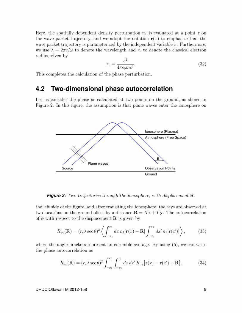
4.2 Two-dimensional phase autocorrelationLet us consider the phase as calculated at two points on the ground, as shown inFigure 2. In this figure, the assumption is that plane waves enter the ionosphere on

Ground

Ionosphere (Plasma)

Atmosphere (Free Space)

Source Observation Points Plane waves

R

Figure 2: Two trajectories through the ionosphere, with displacement R.

the left side of the figure, and after transiting the ionosphere, the rays are observed attwo locations on the ground offset by a distance R = Xx + Y y. The autocorrelationof φ with respect to the displacement R is given by

Rφ1(R) = (reλ sec θ)2⟨∫ x1

−x1dxn1[r(x) + R]

∫ x1

−x1dx′ n1[r(x′)]

⟩, (33)

where the angle brackets represent an ensemble average. By using (5), we can writethe phase autocorrelation as

Rφ1(R) = (reλ sec θ)2∫ x1

−x1

∫ x1

−x1dx dx′Rn1

[r(x)− r(x′) + R

]. (34)


The density autocorrelation Rn1 appearing on the right side is normally defined interms of its Fourier transform, which we can write as

Rφ1(R) =(reλ sec θ)2

(2π)3

∫ x1

−x1

∫ x1

−x1dx dx′

∫ ∞−∞

∫ ∞−∞

∫ ∞−∞

dκSn1(κ)eiκ·[r(x)−r(x′)+R]. (35)

Next, we change the order of integration:

Rφ1(R) =(reλ sec θ)2

(2π)3

∫ ∞−∞

∫ ∞−∞

∫ ∞−∞

dκSn1(κ)eiκ·R∫ x1

−x1

∫ x1

−x1dx dx′ eiκ·[r(x)−r(x

′)].

(36)We substitute (11) for Sn1 . Since Sn1 ∼ δ(κz), we have κ · [r(x)− r(x′)] = κx(x− x′),and the rightmost double integral is∫ x1

−x1

∫ x1

−x1dx dx′ eiκx(x−x

′) =sin2(κxx1)

κ2x= x21 sinc2(κxx1) = (z0 sin 2θ)2 sinc2(κxx1).

(37)The autocorrelation (36) can then be written

Rφ1(R) =4(reλz0 sin θ)2

(2π)2

∫ ∞−∞

∫ ∞−∞

dκxdκy 2π 〈n21〉 sinc2(κxx1)e

iκxX+iκyY

κ20⊥(1 + κ2x/κ20⊥ + κ2y/κ

20⊥)3/2

. (38)

We recall the identity2|x|K1(a|x|)

a=

∫ ∞−∞

dk eikx

(a2 + k2)32

, (39)

where K1 is the modified Bessel function of the second kind. By using (39) we find

Rφ1(R) =8(reλz0 sin θ)2 〈n2

1〉2π

∫ ∞−∞

dκx sinc2(κxx1)κ0⊥|Y |K1

[(κ20⊥ + κ2x)

1/2|Y |]

(κ20⊥ + κ2x)1/2

eiκxX .

(40)Under the condition 105 m ≈ x1 � κ−10⊥ ≈ 104 m, the factor sinc2(κxx1) acts as aDirac delta function with respect to factors of (κ20⊥ + κ2x)

1/2. Hence

Rφ1(R) = 8(reλz0 sin θ)2⟨n21

⟩|Y |K1(κ0⊥|Y |)

1

2π

∫ ∞−∞

dκx sinc2(κxx1)eiκxX . (41)

We note the Fourier transform relationship

1

2π

∫ ∞−∞

dκx sinc2(κxx1)eiκxX =

1

2x1tri

(X

2x1

), (42)

where tri(x) = (1 − |x|)µ(1 − |x|) is the triangle function, and µ(x) is the unit stepfunction. The final form of the correlation function is therefore

Rφ1(R) = 2z0 tan θ(reλ)2⟨n21

⟩tri

(X

2x1

)|Y |K1(κ0⊥|Y |). (43)

This expression is good for two-dimensional displacements R = Xx + Y y. In thenext subsection we extend this result to three-dimensional displacements.


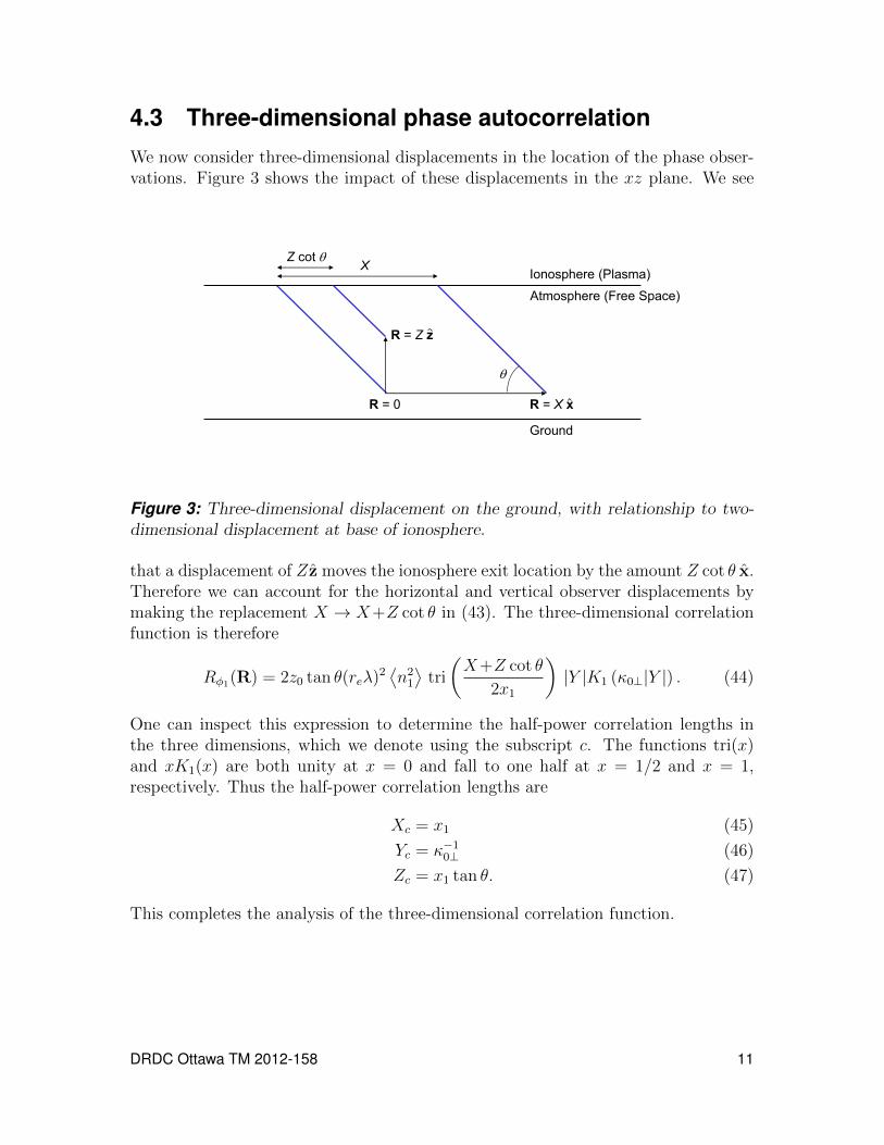
4.3 Three-dimensional phase autocorrelationWe now consider three-dimensional displacements in the location of the phase obser-vations. Figure 3 shows the impact of these displacements in the xz plane. We see

Ground

Ionosphere (Plasma)

Atmosphere (Free Space)

R = 0

X

R = Z z

R = X x

q

Z cot q

Figure 3: Three-dimensional displacement on the ground, with relationship to two-dimensional displacement at base of ionosphere.

that a displacement of Zz moves the ionosphere exit location by the amount Z cot θ x.Therefore we can account for the horizontal and vertical observer displacements bymaking the replacement X → X+Z cot θ in (43). The three-dimensional correlationfunction is therefore

Rφ1(R) = 2z0 tan θ(reλ)2⟨n21

⟩tri

(X+Z cot θ

2x1

)|Y |K1 (κ0⊥|Y |) . (44)

One can inspect this expression to determine the half-power correlation lengths inthe three dimensions, which we denote using the subscript c. The functions tri(x)and xK1(x) are both unity at x = 0 and fall to one half at x = 1/2 and x = 1,respectively. Thus the half-power correlation lengths are

Xc = x1 (45)

Yc = κ−10⊥ (46)

Zc = x1 tan θ. (47)

This completes the analysis of the three-dimensional correlation function.


5 Conclusion

A three-dimensional spatial autocorrelation function for ionospherically propagatedwave packets at high latitudes has been provided. An analytic formula was derivedbased on a linear plasma density profile for the ionosphere and a power-law turbulencespectrum for ionospheric irregularities. The correlation length in the direction normalto the plane of propagation is approximately equal to the outer scale size of plasmairregularities in the ionosphere. The correlation length in the horizontal direction inthe plane of propagation is approximately equal to one-half the horizontal length ofthe ionospheric path transited by the wave packet. The vertical correlation length isshown to be equal to the horizontal correlation length multiplied by the tangent ofthe wave packet take-off angle.

This work provides guidance for interpreting the results of experiments and forproposing future radio systems. In particular, autocorrelation functions provide in-sight on the degree to which ionospheric modes at various elevation and azimuthdirections of arrival can be separated by analysis of the spatial dependent phase.

It would be beneficial to look at the case of general magnetic field dip angle, althoughit does not seem to be analytically tractable at this time. This analysis would supportthe interpretation of results obtained at lower latitudes, and illustrate the quality ofthe approximation of a vertical magnetic field made in the current study.


References

[1] Wheelon, A. D. (2001). Electromagnetic scintillation, Volume 1, geometricoptics. New York: Cambridge University Press.

[2] Tatarskii, V. I. (1971). The effects of the turbulent atmosphere on wavepropagation. Springfield, VA: National Technical Information Service.

[3] Rufenach, C. L. (1975). Ionospheric scintillation by a random phase screen:spectral approach, Radio Sci., 10 (2), 155–165.

[4] Coleman, C. J. (1996). A model of HF sky wave radar clutter, Radio Sci., 31(4), 869–875, doi:10.1029/96RS00721.

[5] Ravan, M., Riddolls, R. J., Adve, R. S. (2012). Ionospheric and auroral cluttermodels for HF surface wave and over the horizon radar systems, Radio Sci., 47,doi: 10.1029/2011RS004944.

[6] Dana, R., Wittwer, L. A. (1991). A general model for RF propagation throughstructured ionization, Radio Sci., 26 (4), 1059–1068, doi:10.1029/91RS00263.

[7] Nickisch, L. J. (1992). Non-uniform motion and extended media effects on themutual coherence function: an analytic solution for spaced frequency, position,and time, Radio Sci., 27 (1), 9–22.

[8] Knepp, D. L. (1983). Analytic solution for the two-frequency mutual coherencefunction for spherical wave propagation, Radio Sci., 18 (4), 535–549.

[9] Gherm, V. E., Zernov, N. N., Strangeways, H. J. (2005). HF propagation in awideband ionospheric fluctuating reflection channel: physically based softwaresimulator of the channel, Radio Sci., 40 (1), 1–15, doi:10.1029/2004RS003093.

[10] Rytov, S. M., Kravtsov, Y. A., Tatarskii, V. I. (1989). Principles of statisticalradiophysics, Volume 4, wave propagation through random media. Berlin,Germany: Springer.

[11] Budden, K. G. (1985). The propagation of radio waves: the theory of radiowaves of low power in the ionosphere and magnetosphere. New York:Cambridge University Press.

[12] Kelley, M. C. (1989). The Earth’s ionosphere. San Diego: Academic Press.

[13] Woodman, R. F., Basu, S. (1978). Comparison between in-situ spectralmeasurements of F-region irregularities and backscatter observations at 3mwavelength, Geophys. Res. Lett., 5, 869–872, doi:10.1029/GL005i010p00869.

[14] Vallieres, X., Villain, J. P., Hanuise, C., Andre, R. (2004). Ionosphericpropagation effects on spectral widths measured by Superdarn HF radars, Ann.Geophys., 22, 2023–2031.


DOCUMENT CONTROL DATA(Security classification of title, body of abstract and indexing annotation must be entered when document is classified)

1. ORIGINATOR (the name and address of the organization preparing thedocument. Organizations for whom the document was prepared, e.g. Centresponsoring a contractor’s report, or tasking agency, are entered in section 8.)

Defence R&D Canada – Ottawa3701 Carling Avenue, Ottawa, Ontario, CanadaK1A 0Z4

2. SECURITY CLASSIFICATION(overall security classification of thedocument including special warning terms ifapplicable).

UNCLASSIFIEDDMC: AREVIEW GCEC: April 2011

3. TITLE (the complete document title as indicated on the title page. Its classification should be indicated by the appropriateabbreviation (S,C,R or U) in parentheses after the title).

The three-dimensional spatial autocorrelation of ionospherically propagated wave packets athigh latitudes

4. AUTHORS (last name, first name, middle initial)

Riddolls, Ryan J.

5. DATE OF PUBLICATION (month and year of publication ofdocument)

December 2012

6a. NO. OF PAGES (totalcontaining information.Include Annexes,Appendices, etc).

23

6b. NO. OF REFS (totalcited in document)

14

7. DESCRIPTIVE NOTES (the category of the document, e.g. technical report, technical note or memorandum. If appropriate, enter thetype of report, e.g. interim, progress, summary, annual or final. Give the inclusive dates when a specific reporting period is covered).

Technical Memorandum

8. SPONSORING ACTIVITY (the name of the department project office or laboratory sponsoring the research and development.Include address).

Defence R&D Canada – Ottawa3701 Carling Avenue, Ottawa, Ontario, Canada K1A 0Z4

9a. PROJECT NO. (the applicable research and developmentproject number under which the document was written.Specify whether project).

13mz08

9b. GRANT OR CONTRACT NO. (if appropriate, the applicablenumber under which the document was written).

10a. ORIGINATOR’S DOCUMENT NUMBER (the officialdocument number by which the document is identified by theoriginating activity. This number must be unique.)

DRDC Ottawa TM 2012-158

10b. OTHER DOCUMENT NOs. (Any other numbers which maybe assigned this document either by the originator or by thesponsor.)

11. DOCUMENT AVAILABILITY (any limitations on further dissemination of the document, other than those imposed by securityclassification)( X ) Unlimited distribution( ) Defence departments and defence contractors; further distribution only as approved( ) Defence departments and Canadian defence contractors; further distribution only as approved( ) Government departments and agencies; further distribution only as approved( ) Defence departments; further distribution only as approved( ) Other (please specify):

12. DOCUMENT ANNOUNCEMENT (any limitation to the bibliographic announcement of this document. This will normally correspondto the Document Availability (11). However, where further distribution beyond the audience specified in (11) is possible, a widerannouncement audience may be selected).

Unlimited

13. ABSTRACT (a brief and factual summary of the document. It may also appear elsewhere in the body of the document itself. It is highlydesirable that the abstract of classified documents be unclassified. Each paragraph of the abstract shall begin with an indication of thesecurity classification of the information in the paragraph (unless the document itself is unclassified) represented as (S), (C), (R), or (U).It is not necessary to include here abstracts in both official languages unless the text is bilingual).

We analytically derive a three-dimensional spatial autocorrelation function for the phase of iono-spherically propagated wave packets at near-vertical magnetic field dip angles. The correlationlength in the direction normal to the plane of propagation is approximately equal to the outerscale size of plasma irregularities in the ionosphere. The correlation length in the horizontal direction in the plane of propagation is approximately equal to one-half the horizontal length of the ionospheric path transited by the wave packet. The vertical correlation length is shown to be equal to the horizontal correlation length multiplied by the tangent of the wave packet take-off angle.

Nous développons analytiquement une fonction d’autocorrélation tridimensionnelle pour la phase de paquets d’ondes à propagation ionosphérique à des angles d’inclinaison du champ magnétique presque verticaux. La longueur de corrélation dans la direction normale au plan de propagation est environ égale à la taille des plus grandes irrégularités plasmatiques de l’ionosphère. La longueur de corrélation dans la direction horizontale du plan de propagation est environ égale à la moitié de la longueur horizontale du trajet ionosphérique suivi par le paquet d’ondes. On montre que la longueur verticale de corrélation est égale à la longueur de corrélation horizontale multipliée par la tangente de l’angle de rayonnement du paquet d’ondes.

14. KEYWORDS, DESCRIPTORS or IDENTIFIERS (technically meaningful terms or short phrases that characterize a document and couldbe helpful in cataloguing the document. They should be selected so that no security classification is required. Identifiers, such asequipment model designation, trade name, military project code name, geographic location may also be included. If possible keywordsshould be selected from a published thesaurus. e.g. Thesaurus of Engineering and Scientific Terms (TEST) and that thesaurus-identified.If it not possible to select indexing terms which are Unclassified, the classification of each should be indicated as with the title).

radiosky wavehigh frequencyionospherecorrelationscintillation

the three-dimensional spatial autocorrelation of...

Documents