“the thirty dollar drop” - yale university

of 36

“The Thirty Dollar Drop”: A Study of (1) Risk Aversion, (2) “Perceived Control” Effect, (3) Under-

and Over-Confidence, and (4) Hindsight Bias in “Hedged” Decisions

Daniel H. Stern* | April 2016 | CGSC 491: Senior Thesis in

Cognitive Science ‡

* Daniel Stern is a senior undergraduate at Yale University, majoring in Cognitive Science.

Within the major, he studies decision-making, strategy, and persuasion.

‡This research is, at present, submitted in partial fulfillment of the requirements of the

Cognitive Science major. It is, however, an ongoing collaboration between the author and

Professor Shane Frederick of Yale School of Management. I am happy to make the data

set available to any readers—and to field comments or questions—at [email protected]

mailto:[email protected]

of 36

ABSTRACT

This paper extends prior behavioral economics findings—of risk aversion, “perceived

control” effects, difficulty-dependent overconfidence and underconfidence, and

hindsight bias – to the novel decision domain of “bet hedging.” It identifies and

integrates all of these biases using a single experimental paradigm, inspired by TV’s

The Million Dollar Drop game show.

In our experiment, subjects wagered or spread real money on mutually exclusive

probabilistic outcomes or trivia answers, only retaining money placed on the correct

outcome. Our paper reports the following findings:

First, subjects were quite risk-averse in their allocations, eschewing the EV-

maximizing strategy of the task in order to lower their outcome variance. Less than

5% of subjects stuck always to the task’s EV-maximizing strategy; less than half of

subjects even played the EV-maximizing strategy on over 50% of individual rounds.

Subjects were especially risk-averse in their first wager in each experimental block,

when they had lots of money to hedge.

Second, subjects’ allocation strategies were irrationally influenced by “perceived

control” effects, with subjects behaving with higher risk aversion when they lacked

“perceived control” over the outcome of their wagers, even when all other features of

their situations were formally identical.

Third, replicating the results of research by Moore and Healy (2007), subjects were

found to be overconfident in their own skill on high-difficulty trivia questions, but

underconfident in their skill on low-difficulty questions – supporting a difficulty-

dependent model of overconfidence and underconfidence.

Finally, incidental to the allocation patterns themselves, subjects demonstrated

hindsight bias after completing the experiment: their memory of subjective

probabilities that they’d previously provided for trivia answers was influenced by

whether or not they’d subsequently learned the answers to be correct.

of 36

INTRODUCTION

This paper turns a very simple task into a wealth of research on human decision-making

and hedging behavior.

Inspired by TV’s The Million Dollar Drop [see Appendix A], we study how decision-

makers choose to allocate money across mutually exclusive possibilities. Namely,

decision-makers in the real world often face competing investments that are mutually

exclusive but jointly comprehensive: e.g., two companies compete in a war of attrition for

a market that can only contain one; two sports teams compete in a game which will have

just one winner; two politicians compete for a single office; and so on.

In these situations, how do investors allocate money across their various options? Do they

spread their money safely, or risk it all on the most likely outcome? Which of these

strategies would actually maximize expected winnings? If one strategy consistently does

maximize expected winnings, do people play this strategy? Or do they sacrifice magnitude

of expected winnings in exchange for less risk? What circumstances change people’s

allocation behavior? What circumstances bring people closest to expected-value

maximizing behavior? Are people capable of accurately assessing outcome probabilities

before betting? In what circumstances do they most and least accurately assess outcome

probabilities? How does hindsight change recollections of prior probability beliefs?

These are all questions that the present paper seeks to answer.

Although no known prior studies use the experimental paradigm featured in the present

paper, this research follows a rich behavioral economics literature which has investigated

similar concepts in non-hedging domains. Specifically, our research seeks to extend and

affirm past behavioral economics concepts—risk aversion, “perceived control bias,”

under- and over-confidence, and hindsight bias—in the novel “hedging” domain. To

understand the results of this study, then, some background in these key concepts is

necessary. These topics will be much better recapped and explored further in the body of

the paper, as each concept becomes relevant, but the following can serve as an introduction

to the naïve reader. These concepts can skipped over by the already familiar, as the body

of the paper will provide more coverage of them.

Background Concept #1: Expected Value

“Expected value” (EV) is one of the classic concepts in economics, which allows

computation of the average returns on a probabilistic decision. (Huygens 1714.) It’s

calculated as the sum of all possible payoffs weighted by their probabilities of coming to

fruition. Economists often contend that a basic rule of choosing a successful strategy or

making a correct decision is to identify the decision that will maximize expected value.

(Dixit & Nalebuff, 2008.)

Behavioral economics, the field to which this paper belongs, often seeks to identify areas

of 36

in which real people deviate from the EV-maximizing behavior that might be predicted by

classical economic theory. (Kahneman et. al. 1991, Kahneman 2003.)

Background Concept #2: Risk Aversion

One reason that a human actor might choose not to maximize expected value is because

of a preference against risk. “Risk aversion” is the idea that humans frequently sacrifice

expected value in order to reduce the variance between possible outcomes. (Bernoulli

1954, Van Der Meer 1963.) In other words, between accepting a 50% chance of $100

and a 100% guarantee of $50, there is technically no difference in expected value.

However, the two cases clearly have great difference in outcome variance. Sometimes,

reducing outcome variance—e.g. choosing the sure bet over the risky bet—also does

reduce expected winnings. Such will be the case in the present paper. When people

choose security over value in such a tradeoff, we say that they’re displaying “risk

aversion.”

Background Concept #3: “Perceived Control” Effect

In many fields studied by behavioral psychologists—ranging from medicine, to education,

to mood, to consumer choice—research has found that people act differently in formally

identical situations when they “perceive that they have control” over the outcomes of the

situations. (Wallston et. al., 1987; Klein et. al., 2010; Hui and Bateson, 1977; Skinner &

Wellborn, 1990; Langer 1975.) For example, according to one study by Hui and Bateson

(1977), holding constant a service employee’s actual behavior towards a customer, the

customer’s perception of whether or not he has “control” over the start and termination of

the employee-customer relationship has an effect on his judgment of the employee’s

behavior. In a study by Skinner and Wellborn (1990), randomly assigned stories of whether

or not students could ‘control’ their educational success influenced their motivation and

response to formally identical lessons. And in betting situations, introducing an element of

skill to a probabilistic decision—while not changing the underlying payoffs or

probabilities—has been shown to influence the decision. (Langer 1975.) In other words,

sometimes, when we feel we have active control over an outcome, our behavior changes

even if situations are otherwise identical.

Background Concept #4: Overconfidence and Underconfidence

Behavioral economics has many times proven that we are not accurate judges of our own

skill. Instead, on many tasks, we have been demonstrated as predictably overconfident.

(Kahneman 2011; Alba & Hutchinson 2000; Odean 1998; Barber & Odean 2001.) On other

tasks, we have been demonstrated as predictably underconfident. (Griffin & Tversky 1992;

Larrick et. al. 2007.) A recent paper by Moore and Healy (2007) reconciled these two

disparate literatures by referencing the difficulty of the tasks, creating a unified model that

will be discussed in subsequent sections of the present paper.

of 36

Background Concept #5: Hindsight Bias

Hindsight bias, from psychology, references the changes in remembered subjective

probability or remembered decision framework that occur after an outcome is known.

(Roese and Vohs, 2012; Pennington 1981; Zwick et. al. 1995; Goodwill et. al. 2010;

Henriksen & Kaplan, 2003.) For example, prior to 9/11, security officials in the United

States had some estimation of the likelihood of a mass terrorist attack. Since it’s happened,

citizens now frequently attempt to remember our estimated likelihood (prior to the event)

of an upcoming mass terrorist attack. The literature of hindsight bias suggests that these

two likelihoods—the one actually estimated prior to the event, and the remembered

estimate—are different, with the remembered estimate being biased by hindsight and by

the event’s actually having occurred.

Final Introductory Notes

Armed with knowledge of these background concepts, it should be possible to understand

and wade through the experimental method, results, and analysis detailed below. While

risk aversion, “perceived control” effect, overconfidence and underconfidence, and

hindsight bias have been extensively studied in general, they haven’t—to our knowledge—

been applied to laboratory bet-hedging studies like the present. Most extant research on

hedging has come in a financial markets context, e.g. with observations of factors that lead

major finance firms to hedge, or with claims that investors may misunderstand the purpose

of asset diversification. (Reinholtz et. al., 2016; Smith et. al., 1985; Stulz et. al., 1984.) We

hope, though, that this study will be among the first of many to study individual-level

hedging in a laboratory setting.

of 36

METHODS AND DATA

281 subjects were recruited for our study, carried out in Yale School of Management’s

Behavioral Lab. All 281 subjects participated in our “Condition A,” and were additionally

randomly assigned to participate in either “Condition B” or “Condition C.” The order in

which the conditions were presented, for each subject, was randomized.

At the beginning of the study, subjects were promised $5 for participation, and an

opportunity to win up to an additional $60. This $60 could be won over the course of each

subject’s two conditions in the experiment, with a maximum $30 of winnings in each. At

the beginning of each condition, subjects were credited a new $30 and told that they’d be

making a seven-round series of economic decisions and/or wagers with this credited

money, in each of which rounds they stood to lose all, part, or none of their remaining

money. At the end of these seven rounds, they were told, they’d keep whatever money they

had remaining from that condition, before proceeding to their second assigned condition.

Condition A: Objective Probabilities

In Condition A, subjects went through rounds of wagering their money on two

mutually exclusive “outcomes” with objective probabilities of occurring.

Subjects were given complete information about the two possible “outcomes” in each

round. For example, subjects could be told that “Outcome 1” had a 40% chance of

occurring while “Outcome 2” had a 60% chance of occurring, or that “Outcome 1” had a

90% chance of occurring while “Outcome 2” had a 10% chance of occurring, and so on.

[Probabilities assigned to each outcome were randomly generated, but always summed to

100% in each round.]

Subjects were then asked to wager all of their money (beginning in the first round w/ $30)

across either or both of the outcomes, knowing that they would keep for the next round

only the money that was placed on the correct outcome. Subjects could place all money

on one outcome, or split it across both. But subjects were—every round—required to put

each dollar of their remaining money somewhere.

After subjects spread their money across the two outcomes, a random number generator

selected the “winning” outcome using the probabilities given. All money placed on the

“winning” outcome was retained by the subject for the next round; all money placed on the

“losing” outcome was lost. After seven rounds, subjects were paid out all money that they

hadn’t yet lost. If a subject lost all his money before the end of the seventh round, the

condition ended immediately with the subject receiving no added money (beyond the total

$5 of participation) for the condition. Allocations and winnings in each of the seven rounds

was recorded for later analysis.

Allocations were analyzed for subject strategy relative to EV-maximizing behavior, and

strategy relative to other conditions in the experiment. All text and screens presented to

of 36

subjects in Condition A are included in Appendix B.

Condition B: Trivia With In-Round Requests for Subjective Probabilities

In Condition B, subjects went through rounds of wagering their money on two

mutually exclusive multiple choice trivia answers.

In each round in Condition B, subjects were presented with two randomly generated

U.S. states, and then asked to bet on which of the states was bigger (in either state

area or population, also a randomly generated parameter of the condition). Subjects

were asked to wager all of their money across either or both of the two states, knowing that

they would keep for the next round only the money placed on the correct answer. As before,

subjects could place all money on one outcome, or split it amongst both. Subjects were, as

in Condition A, required to put each dollar of their remaining money on one of the answer

choices.

Before making the wagers, though, subjects were also asked how likely they thought each

answer choice was of being correct. In other words, before betting, say, $30 on Florida and

$20 on Georgia, subjects were asked to indicate how likely (in “% likely”) they believed

each of the state trivia answer choices was to be correct.

After spreading their money across the two U.S. state answer-choices, the correct trivia

answer was revealed. All money placed on the correct answer was retained by the subject

for the next round; all money placed on the incorrect answer was lost. After seven rounds,

subjects were paid all money they hadn’t yet lost. As in Condition 1, if a subject lost all

money before the end of the seventh round, the experimental block ended without bonus

compensation for the subject. Allocations and winnings in each round were recorded for

later analysis, as was the difficulty of each problem (coded by the ratio of area or population

numbers between the two states).

Additionally, in Condition B, subjects were asked after completing all rounds to provide

their pre-wager subjective probabilities for each of the multiple choice answers they faced

during the experiment. In plain English, they were asked to indicate how likely they had

previously thought (before learning the correct answer) each multiple choice possibility

was to be correct. These remembered subjective probabilities were also recorded for later

analysis.

Allocations were analyzed for subject strategy relative to EV-maximizing behavior,

strategy relative to other conditions in the experiment, and the relationship between

confidence and accuracy. End-of-experiment “remembered” subjective probabilities were

also compared to subjective probabilities given before the corrected answers were learned.

All text and screens presented to subjects in Condition B are included in Appendix C.

of 36

Condition C: Trivia Without In-Round Requests for Subjective Probabilities

Condition C was exactly like Condition B, except that subjects were NOT asked to

give their subjective probabilities for each trivia answer before wagering their money

in each round. Probabilities, therefore, were presumably less salient to subjects as they

made their wagers.

The rest of the procedure in Condition C exactly mirrored that in Condition B, including

the questionnaire after the final round asking subjects to, in this case, state for the first time

their prior subjective probability assessments.

Again, all data was preserved for later analysis, of similar types to that in Conditions A and

B.

All text and screens presented to subjects in Condition C are included in Appendix D.

---

All data analysis for this paper was done using the R statistical computing language within

an R Studio interface. Funding was generously provided by Yale School of Management’s

Behavioral Sciences Laboratory. Lab manager Jessica Halten and programmer Steven

McLean assisted with the implementation of the above methodology.

In total, the 281 subjects made 3,126 wagers. Subjects earned an average of $6.54 during

the experimental blocks themselves, so an average of $11.54 including the $5 participation

bonus. The study, in whole, paid out $3,242 of winnings. Data will be preserved for future

research and is available upon request of the author.

R scripts used to generate the results detailed below are also available upon request of the

author.

of 36

RESULT 1: RISK AVERSION

As our first result, we find that subjects frequently demonstrate risk aversion in their money

allocations—across all three conditions of the experiment—and often deviate from the

“expected-value-maximizing” strategy of these hedging situations. Whereas maximizing

expected value would involve “going all in” on one answer, we see essentially no subjects

who always play their expected-value-maximizing strategy, and instead observe that over

50% of subjects “go all in” on fewer than half of their bets. Instead of “going all in”,

subjects frequently opt for more risk averse distributions that sacrifice expected value in

exchange for reduced outcome variance.

What is This Game’s “EV-Maximizing Strategy”?

Subjects in our experiment are asked to wager money on either or both of two possible

answer choices. Counterintuitively, the strategy that maximizes a subject’s expected

winnings in this task is to always place all remaining money on the outcome or trivia

answer thought more likely to be correct. Regardless of whether a subject is 100%

confident, 80% confident, 60% confident, or even just 51% confident in one choice over

another, if one answer/outcome is any more likely to be correct than the other, a subject’s

EV-maximizing strategy is to put all remaining money on that outcome/answer, leaving

none on the less likely one.

To make this more intuitive, consider cases where a subject is 80% confident in

Answer/Outcome A and 20% confident in Answer/Outcome B. For every dollar placed on

Answer/Outcome A, 80 cents of returns are expected; for every dollar placed on

Answer/Outcome B, only 20 cents of returns are expected. In other words, for every dollar

placed on the less likely answer/outcome, 60 cents of expected value are sacrificed. And

this logic extends to any distribution of probabilities. When each dollar is associated with

an estimated probability of being retained, expected value is lost when dollars are moved

from more probable answers to less probable answers. It becomes clear, then, that EV is

maximized in this task by going “all in” on one answer/outcome in every round.1

Results: Subject Behavior is Risk-Averse Compared to “EV-Maximizing Strategy”

Our data, though, show that subjects do not always act according to this ideal, instead often

hedging their money across the two possible outcomes:

Across all three conditions of our experiment, excluding cases where subjects were “100%

1 One exception to this comes when a subject is dead split (e.g. completely indifferent) between both

outcomes/answers. If a subject can’t identify either outcome/answer as more probable, no allocation of

money across the two tied options at all changes the contestant’s expected returns: if the probabilities are

estimated as the same for both answers, after all, dollars placed on each produce identical expected returns.

This is only the case in perfect ties, though; in all other cases, subjects maximize EV by putting all money

on the most likely outcome.

of 36

confident” in a particular outcome, 61% of subjects’ wagers featured hedged bets, thus

deviating from EV-maximizing behavior.

And in the first bet of each experimental block—e.g. when subjects had the full $30 to

wager, and hadn’t yet experienced losses from hedging in that round—this number was

even more staggering: 78% of wagers in the first bet of each block were hedged, again

sharply deviating from EV-maximizing behavior.

Far from subjects always playing their EV-maximizing strategy, “hedging” was prevalent

in each of our three conditions, for all levels of confidence except when subjects were

100% confident in one or the other answer. (Even when subjects were 90% confident in

one of the outcomes, they still hedged at least a little bit of money over 40% of the time,

losing 80 cents of expected value per dollar hedged.)

But how much money, exactly, was hedged? How much deviation was typical from the

EV-maximizing strategy? The images below capture the story nicely.

Figure 1, below, shows what a graph of average wager on Answer A (in terms of

proportion of money remaining) vs. confidence in Answer A would look like if subjects

were actually playing their EV-maximizing strategy.

Figure 1: The expected-value maximizing strategy of the task, depicted above, would be to wager 0% of remaining money on any answers that are less than 50% likely, and to wager 100% of remaining money on any answers that

are more than 50% likely.

of 36

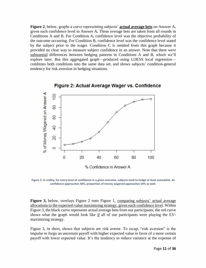
Figure 2, below, graphs a curve representing subjects’ actual average bets on Answer A,

given each confidence level in Answer A. These average bets are taken from all rounds in

Conditions A and B. For Condition A, confidence level was the objective probability of

the outcome occurring. For Condition B, confidence level was the confidence level stated

by the subject prior to the wager. Condition C is omitted from this graph because it

provided no clear way to measure subject confidence in an answer. Note that there were

substantial differences between hedging patterns in Conditions A and B, which we’ll

explore later. But this aggregated graph—produced using LOESS local regression—

combines both conditions into the same data set, and shows subjects’ condition-general

tendency for risk aversion in hedging situations.

Figure 2: In reality, for every level of confidence in a given outcome, subjects tend to hedge at least somewhat. As confidence approaches 50%, proportion of money wagered approaches 50% as well.

Figure 3, below, overlays Figure 2 onto Figure 1, comparing subjects’ actual average

allocations to the expected-value maximizing strategy, given each confidence level. Within

Figure 3, the black curve represents actual average bets from our participants; the red curve

shows what the graph would look like if all of our participants were playing the EV-

maximizing strategy.

Figure 3, in short, shows that subjects are risk averse. To recap, “risk aversion” is the

impulse to forgo an uncertain payoff with higher expected value in favor of a more certain

payoff with lower expected value. It’s the tendency to reduce variance at the expense of

of 36

expected value. When subjects hedge their money across options/answers in this

experiment, they are acting in a “risk-averse” manner because they’re sacrificing expected

value in exchange for lowered variance: they’re moving away from the red curve in Figure

3, which would maximize their EV, and towards safer prospects. To see that the prospects

are safer, consider again a subject who chooses between an Outcome A that is 80% likely

to “win” and an Outcome B that is 20% likely to “win.” For every dollar ‘hedged’ away

from Outcome A, as discussed above, 60 cents of expected value are lost. But for every

dollar ‘hedged’ on B, the difference between the payoffs also becomes two dollars smaller,

reducing the distance between the two possible outcomes. With each dollar wagered on

the less likely outcome/answer, then, subjects are demonstrating definitional risk aversion:

acting to create a more certain payoff of a smaller expected value

Figure 3: There is substantial difference between the EV-maximizing strategy curve of the game (shown in red) and the strategy curve that participants actually use, on average across Conditions A and B (shown in black). When

subjects’ actual behavior deviates from the EV-maximizing red curve, expected value is sacrificed but variance is reduced – this is “risk aversion” by definition.

In our data, subjects became riskier and riskier as they lost more money and went later into

the experiment. Examining only bets made in the first round--with the full $30 still in

play—subjects are even more clearly risk-averse, relative to the experiment’s EV-

maximizing strategy (which is the same in the first round as in all others).

of 36

In Figure 4, below, the EV-maximizing strategy is compared to subjects’ average

allocation strategy in their first bet of Conditions A and B. Note that the allocations deviate

even more from the EV-maximizing strategy, reflecting even higher levels of risk aversion

and even greater sacrifices of expected value than in subsequent rounds of the study.

Figure 4: Looking only at the first wager in each experimental block, subjects are even more risk averse relative to the expected-value maximizing strategy. Consider, for example, answers that subjects have 20% confidence in: if

it’s the first wager of the experimental block, subjects put an average of 20% of their money on these answers that are 80% likely to be incorrect. This represents a substantial loss of expected value. The strategy played on the first wager of each round is more similar to ‘probability matching’ (described below) than to the actual EV-maximizing

strategy of the game.

The wagers made by subjects in the first round of each experimental block are so risk-

averse, in fact, that they closely resemble a “probability-matching” strategy—whereby

subjects wager a proportion of their money on each outcome/answer that is equivalent to

its probability of being the “winning” outcome/answer—than of the actual EV-maximizing

strategy of the game. Note that a probability matching strategy is highly risk averse. It

would suggest placing, for example, 20% of one’s money on an outcome or answer 80%

likely to be incorrect. And this is precisely what we see subjects do, on average, in the first

round of each experimental block.

Though the present experiment is the first [to our knowledge] to use a paradigm with

required simultaneous hedging across answer choices, other variants of “probability-

of 36

matching” strategies have been observed in previous behavioral economics tasks featuring

sequential small-stakes gambles (Vulkan 2000, Koehler and James 2009). This prior work

has shown that, in sequential decision tasks (i.e. tasks where subjects can only bet on a

single probabilistic outcome at a time, but must repeat the same bet many times over), a

majority of subjects match the frequency of their bets on each option with the probabilities

of the various options succeeding. The reason for this tendency seems to be that humans

intuitively [but wrongly] believe that probability-matching is the way to maximize

expected value: multiple studies have found that the “probability matching” tendency in

gamblers can be eliminated if a subject is told that the “EV-maximizing strategy” is

something other than ‘matching,’ indicating that subjects had originally thought

probability-matching would maximize EV. (Koehler and James, 2009.) This may explain

our present study’s subjects’ tendency to play this strategy in the first round of each

experimental block. Regardless, it is extremely risk averse.

Comparing Condition B to Condition C

One purpose of running Condition C—where subjects wagered money on trivia answers

without first stating their confidence in those trivia answers—was to compare allocation

strategies in Condition B with those in Condition C. Specifically, we hypothesized that

with probabilities not made as salient, a higher number of Condition C participants than

Condition B participants would go “all in” on their preferred answer. We hypothesized that

a smaller number of participants would “probability match” in Condition C than Condition

B. However, we found no significant differences between allocation strategies in

Condition B and Condition C. The decreased salience of probabilities in Condition C did

nothing to change hedging behavior: subjects were similarly risk averse in Condition C as

in Condition B.

Discussion: Is This Behavior Rational?

Risk aversion isn’t necessarily irrational. Von Neumann and Morganstern’s famous theory

of “expected utility” (Von Neumann and Morgenstern, 1944) notes that not every dollar is

worth the same amount of usefulness or happiness to its owner. Diminishing marginal

utility does—and perhaps should—imply some amount of risk aversion. There’s also no

final answer as to how much risk aversion is too much: rational risk aversion depends on

one’s own marginal utility function. But we can comment on how risk averse particular

decisions are. Relative to the EV-maximizing strategy, in Conditions A and B of our

experiment, we can say that subjects act in a quite risk-averse manner in situations with

mutually exclusive possible bets and an option to hedge. They act especially risk-averse—

using roughly a probability matching strategy—when they have the full $30, in the first

trial of each block.

This result, overall, is highly consistent with the behavioral economics literature. Time and

again, the field’s literature has found that we are risk averse decision-makers: that, whether

it’s rational (because of VNM expected utility) or irrational (e.g. a habit that we should try

of 36

to override), we sacrifice expected value in exchange for higher outcome certainty.

(Bernoulli 1954; Pratt 1964; Holt & Laury 2002.) This finding is extended, here, with the

present novel hedging paradigm.

RESULT 2: “PERCIEVED CONTROL” EFFECT

While there was risk aversion across all three conditions—relative to the EV-maximizing

strategy of the game—allocation strategies were significantly different in Condition A

than in Conditions B and C.

These differences are potentially explicable by what the literature, as cited in the intro, has

called a “perceived control” effect: even when the situations were formally the same,

people adjusted their hedging allocations when they felt that the outcomes were out of their

control [and instead determined by a computer or random number generator] in Condition

A, relative to when their own skill controlled their fate in Condition B.

Psychological Differences Between Condition A and Condition B

Although Condition A and Condition B feature formally the same task—allocating money

across mutually exclusive options with known (Condition A) or estimated (Condition B)

probabilities of cashing out—there still seems a substantial psychological difference

between betting on one’s own knowledge, as in Condition B, and betting on the result of a

computerized number generator, as in Condition A.

In other words, a subject in Condition A might know, for example, that there’s an 80%

likelihood of Outcome 1 and a 20% likelihood of Outcome 2. But, after placing his wagers

on Outcome 1 and Outcome 2, the subject has no control over his fate: he forfeits agency

to the number generator.

In contrast, a subject who estimates with 80% confidence that State A has a larger

population than State B controls his fate throughout the entire experiment. He places bets

and earns whatever he earns because of his own skill at the task.

Rationally, there should be no difference in bet allocation between these two scenarios. In

both cases, an economic actor is faced with the same possible investments with the same

estimated probabilities of coming to fruition. But psychologically, there seems a huge

difference between the scenarios. We hypothesized that this psychological difference

would affect betting allocation.

Results: Subjects Are Far More Risk-Averse When They Don’t Control Their Fate

of 36

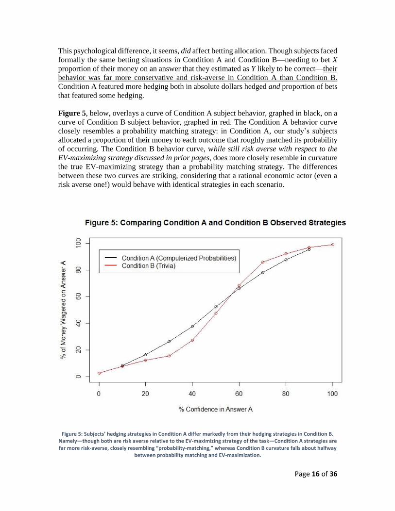
This psychological difference, it seems, did affect betting allocation. Though subjects faced

formally the same betting situations in Condition A and Condition B—needing to bet X

proportion of their money on an answer that they estimated as Y likely to be correct—their

behavior was far more conservative and risk-averse in Condition A than Condition B.

Condition A featured more hedging both in absolute dollars hedged and proportion of bets

that featured some hedging.

Figure 5, below, overlays a curve of Condition A subject behavior, graphed in black, on a

curve of Condition B subject behavior, graphed in red. The Condition A behavior curve

closely resembles a probability matching strategy: in Condition A, our study’s subjects

allocated a proportion of their money to each outcome that roughly matched its probability

of occurring. The Condition B behavior curve, while still risk averse with respect to the

EV-maximizing strategy discussed in prior pages, does more closely resemble in curvature

the true EV-maximizing strategy than a probability matching strategy. The differences

between these two curves are striking, considering that a rational economic actor (even a

risk averse one!) would behave with identical strategies in each scenario.

Figure 5: Subjects’ hedging strategies in Condition A differ markedly from their hedging strategies in Condition B. Namely—though both are risk averse relative to the EV-maximizing strategy of the task—Condition A strategies are far more risk-averse, closely resembling “probability-matching,” whereas Condition B curvature falls about halfway

between probability matching and EV-maximization.

of 36

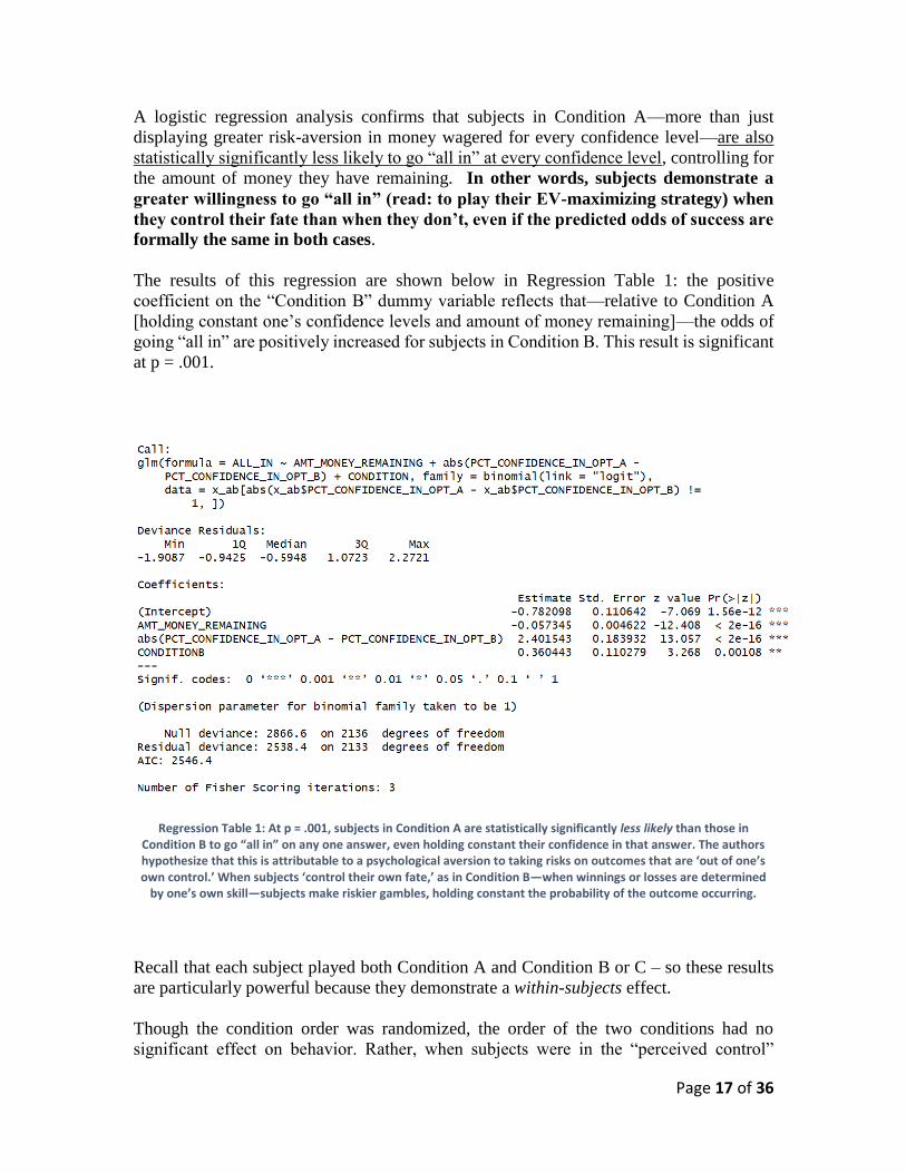
A logistic regression analysis confirms that subjects in Condition A—more than just

displaying greater risk-aversion in money wagered for every confidence level—are also

statistically significantly less likely to go “all in” at every confidence level, controlling for

the amount of money they have remaining. In other words, subjects demonstrate a

greater willingness to go “all in” (read: to play their EV-maximizing strategy) when

they control their fate than when they don’t, even if the predicted odds of success are

formally the same in both cases.

The results of this regression are shown below in Regression Table 1: the positive

coefficient on the “Condition B” dummy variable reflects that—relative to Condition A

[holding constant one’s confidence levels and amount of money remaining]—the odds of

going “all in” are positively increased for subjects in Condition B. This result is significant

at p = .001.

Regression Table 1: At p = .001, subjects in Condition A are statistically significantly less likely than those in Condition B to go “all in” on any one answer, even holding constant their confidence in that answer. The authors hypothesize that this is attributable to a psychological aversion to taking risks on outcomes that are ‘out of one’s own control.’ When subjects ‘control their own fate,’ as in Condition B—when winnings or losses are determined

by one’s own skill—subjects make riskier gambles, holding constant the probability of the outcome occurring.

Recall that each subject played both Condition A and Condition B or C – so these results

are particularly powerful because they demonstrate a within-subjects effect.

Though the condition order was randomized, the order of the two conditions had no

significant effect on behavior. Rather, when subjects were in the “perceived control”

of 36

(trivia) condition, they were more risk-seeking than in the “no perceived control”

(computer-generated probability) condition, regardless of which condition was presented

to them first. Taken together, these results support the hypothesis that – beyond just

probabilities and payoffs – one’s feeling of whether or not one controls an outcome

ultimately affects one’s willingness to take a risk.

RESULT 3: OVERCONFIDENCE AND UNDERCONFIDENCE

As discussed in the introduction, much research in behavioral economics labels humans as

overconfident in their own abilities or performances. (Alba & Hutchinson 2000; Odean

1998; Barber & Odean 2001). But a recent paper by Moore & Healy (2007) has tried to

reconcile overconfidence research with an emerging literature which has found us

sometimes to underestimate our own performance or ability. (Griffin & Tversky 1992;

Larrick et. al., 2007.) Moore and Healy, specifically, hypothesize that we are overconfident

about our performance and skill on difficult tasks, yet underconfident about our

performance and skill on easy tasks.

Using data from the paradigm in the present paper, this hypothesis was testable.

Namely, our Condition B presents subjects with trivia questions that carry objective

measures of difficulty. Because some randomly generated states will be more similar to

others in population and size, some randomly generated questions will necessarily be more

difficult than others. For example, the question of which “Dakota” is larger in area is

objectively more difficult than the question of whether Texas is larger than Delaware. By

creating a ratio of one state’s population or size in comparison to another’s, we rated each

question by its objective difficulty. Note that this isn’t a perfect measure of difficulty –

some states’ sizes are more salient or memorable than others, and so question difficulty

won’t correspond perfectly to size ratio – but it is a good approximation. Then, using the

in-round “subjective probabilities” that subjects submitted in Condition B, we compared

subject’s confidence in their favored answers to their favored answers’ actual performance,

categorizing these comparisons across the entire sample by question difficulty.

Results: Subjects Are Overconfident on Hard Questions, Underconfident on Easy

Questions

Using the method described above, we replicated Moore and Healy’s conclusion exactly.

Namely, our data showed that, on harder questions, subjects underperformed their stated

confidence level; on easier questions, though, they outperformed their stated confidence

level. They were, in other words, overconfident on the hard questions but underconfident

on the easy questions.

Figure 6, below, graphs subjects’ stated confidence and accuracy levels in their preferred

answers for all points on our question difficulty scale. The x-axis, question difficulty,

of 36

measures the ratio of a question’s smaller state area or population to its larger state area or

population: a difficulty of .5, then, means that the question’s smaller state answer choice

had half the population or area of the larger one. When difficulty is very small, it means

that the question compared a huge state to a tiny state (e.g. difficulty of .1 means that the

larger state was 10x bigger than the smaller state); as difficulty approaches 1, the difference

between the two states in population or area approaches zero. Graphed in black are

subjects’ average stated confidence levels in their preferred answers for all points on the

difficulty scale. Graphed in red are the average accuracies of subjects’ preferred answers

for all points on the difficulty scale. Data was smoothed using LOESS local regression.

Figure 6 shows that, when difficulty is low, subjects are more accurate than confident.

When difficulty increases beyond 0.4 (e.g. when the larger state becomes anything less

than 2.5x larger than the smaller state), though, subjects become less accurate than

confident. This exactly confirms Moore and Healy’s hypothesis about difficulty-

dependent overconfidence and underconfidence.

Figure 6: When questions are easy, subjects’ avg. confidence in their favored answer, graphed in black, is lower than their favored answer’s avg. accuracy, graphed in red. But when questions are hard, this trend reverses: on hard questions, subjects are more confident than accurate. This replicates the overconfidence/underconfidence model suggested by Moore and Healy (2007): that people are overconfident in their abilities on hard tasks, but

underconfident in their abilities on easy tasks.

of 36

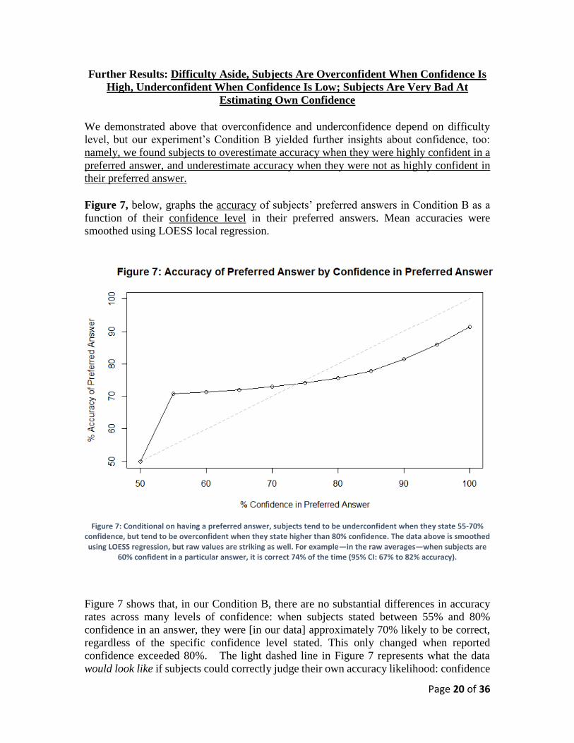
Further Results: Difficulty Aside, Subjects Are Overconfident When Confidence Is

High, Underconfident When Confidence Is Low; Subjects Are Very Bad At

Estimating Own Confidence

We demonstrated above that overconfidence and underconfidence depend on difficulty

level, but our experiment’s Condition B yielded further insights about confidence, too:

namely, we found subjects to overestimate accuracy when they were highly confident in a

preferred answer, and underestimate accuracy when they were not as highly confident in

their preferred answer. Figure 7, below, graphs the accuracy of subjects’ preferred answers in Condition B as a

function of their confidence level in their preferred answers. Mean accuracies were

smoothed using LOESS local regression.

Figure 7: Conditional on having a preferred answer, subjects tend to be underconfident when they state 55-70%

confidence, but tend to be overconfident when they state higher than 80% confidence. The data above is smoothed using LOESS regression, but raw values are striking as well. For example—in the raw averages—when subjects are

60% confident in a particular answer, it is correct 74% of the time (95% CI: 67% to 82% accuracy).

Figure 7 shows that, in our Condition B, there are no substantial differences in accuracy

rates across many levels of confidence: when subjects stated between 55% and 80%

confidence in an answer, they were [in our data] approximately 70% likely to be correct,

regardless of the specific confidence level stated. This only changed when reported

confidence exceeded 80%. The light dashed line in Figure 7 represents what the data

would look like if subjects could correctly judge their own accuracy likelihood: confidence

of 36

would track neatly with accuracy. Instead, our data reveal that subjects have trouble

estimating their own accuracy likelihood beyond just choosing a preferred answer;

subjects are thus overconfident in their preferred answers when confidence is

relatively high and underconfident when confidence is relatively low.

The flatness of the curve in Figure 7 is admittedly somewhat hard to believe—and certainly

is worth retesting with larger samples—but the sample size in the present experiment is

sufficient to conclude that when we perceive slight confidence advantages for one trivia

answer over another (e.g. 60% confident in Answer A, 40% confident in Answer B), our

preferred answer is correct at higher accuracy rates than we project; and, conversely, when

we perceive huge confidence advantages for one answer over another, our preferred answer

is correct at lower accuracy rates than we project.

For example, when subjects stated 60% confidence in a trivia answer, they were correct

74% of the time. A one-sample t-test reveals, with 95% statistical certainty, that the true

population of people stating 60% confidence in a trivia answer would be picking the correct

answer between 67% and 82% of the time. For other indicated confidence levels below

75% (.55, .65, .7), one-sample t-tests reveal similar statistically significant

underconfidence. On the other hand, for stated confidence levels above 75% (.8, .9, .95),

t-tests reveal statistically significant overconfidence.

While the bizarre flatness in our results’ mean accuracy rates for answers with 55%-80%

stated confidence, then, may be mere noise in our data, the fact of underconfidence on

confidence levels between 50-70% and overconfidence on confidence levels between 80-

100% is valid.

RESULT 4: HINDSIGHT BIAS

Hindsight bias is described well in the literature, in a review paper by Roese and Vohs

(2012), as:

“[the bias] when people feel that they ‘knew it all along’—that is, when they believe

an event is more predictable after it becomes known than it was before it became

known.”

Well-reported and replicated by many prior papers (Pennington 1981; Zwick et. al. 1995;

Goodwill et. al. 2010), hindsight bias often involves misremembering prior judgements of

an event’s probability after the event does or doesn’t come to fruition.

The data from the experimental paradigm used in this paper can support an extension

of hindsight bias into the domain of hedging. Specifically, Conditions B and C in the

present experiment allow us to test the hypothesis that hindsight bias affects judgements of

prior subjective probabilities. This is because Conditions B and C both asked subjects to

recall, after the experiment was over, how probable they had thought each answer choice

of 36

was prior to learning the correct answer. In the case of Condition B, we can test for

movement between the prior stated probabilities and these post-experiment recollections,

checking for an effect of answer correctness. In the case of Condition C (where subjects

didn’t give subjective probabilities before betting), we can test for whether, holding

constant the proportion of money that had been wagered on an answer, an answer’s

correctness changes a subject’s recalled subjective probability for that answer.

Results: Hindsight Affects Memory of Subjective Probability

Using simple least squares regression, we first tested the effect of hindsight on remembered

subjective probability in Condition B. Given that Condition B asked subjects to provide

subjective probabilities before making wagers or learning the correct answer, and then to

provide remembered subjective probabilities after the experiment was over, it was easy to

test for movement on the basis of hindsight or learned information.

Regression Table 2 shows the result of this regression: namely, hindsight did affect

subjects’ remembered subjective probabilities. Holding constant their earlier

estimations of probability for an answer choice, the answer choice’s correctness changed

remembered subjective probability by almost 10 percentage points. In other words, when

an answer was later learned to be correct, subjects recalled believing, on average, that it

was almost 10 percentage points more probable than they recalled believing it was when

they later learned it to be false, holding constant what they actually had previously

indicated. The coefficient of interest, here, is OPT_A_CORRECTTRUE, which [relative

to learning that the answer was false] influences later remembered probability by .096. This

hindsight effect is significant at p < .0001.

Regression Table 2: At p < .0001, learning that a particular answer choice is true [or false] affects later remembered subjective probability of the answer choice, holding constant the subjective probabilities that subjects had

previously stated for the answer choice. Hindsight moves remembered subjective probability towards the truth.

of 36

We were able to probe this effect using data from Condition C, too. Though Condition C

subjects didn’t state subjective probabilities prior to placing their bets or learning the true

answers, we could compare the Condition C subjects’ “recalled subjective probabilities”

based on hindsight, holding constant the proportion of money that they had previously

wagered on answers. The hindsight effect here, then, isn’t as clean as the one found in

Condition B subjects. But the hypothesized effect was found nonetheless, and the data

actually showed a stronger effect in Condition C than Condition B.

Regression Table 3 shows the results of this regression, which found that—holding

constant the proportion of a subject’s money that he had allocated to an answer choice—

whether or not that answer choice turned out to be correct affected his post-experiment

memory of that answer choice’s subjective probability by 15 percentage points.

Regression Table 3: In condition B, at p < .0001, learning that a particular answer choice is true [or false] affects later remembered subjective probability of the answer choice, holding constant the proportion of one’s money

that one had chosen to wager on that answer choice. The effect size in this regression is larger than the effect size in the previous hindsight regression, potentially indicating that hindsight bias is more pronounced when subjects

don’t explicitly consider—a priori—subjective probabilities for outcomes.

That the hindsight effect size is bigger in the Condition C regression than the

aforementioned Condition B regression [and bigger in Condition C regression than in a

second Condition B regression which uses the Condition C model: controls for proportion

of money wagered on an answer rather than prior subjective probability] could indicate

that the hindsight effect is larger when subjects don’t explicitly consider subjective

probabilities prior to learning results. In terms of ecological application, then, we might

suggest thinking in probabilistic terms before learning the results of decisions. This could

minimize one’s hindsight bias, though our results indicate that it certainly won’t eliminate

it.

of 36

CONCLUSION

In sum, this paper reaffirms long-standing behavioral economics principles in a new

decision-making context with a novel task: a task involving hedging across mutually

exclusive outcomes.

It shows, first and foremost, that subjects substantially deviate from EV-maximizing

behavior in the mutually-exclusive hedging situations captured by the experiment. They

particularly deviate from EV-maximizing behavior in early bets of the experiment, when

they have plenty of money remaining to hedge with.

It shows, second, that this risk-averse behavior is amplified when subjects lack “perceived

control” over the outcomes of their wagers. Even faced with formally identical situations,

subject allocation strategy is wildly different in trivia vs. number generator conditions, with

number generator conditions eliciting probability-matching levels of risk aversion.

It replicates, third, the Moore & Healy (2007) finding that subjects are underconfident in

their skill on easy tasks, yet overconfident in their skill on hard tasks. In so doing, it extends

these results to the hedging domain. It further reports in the area of overconfidence and

underconfidence that subjects’ accuracy outperforms their confidence for confidence levels

between 55% and 70%, but underperforms their confidence for confidence levels between

80% and 100%.

It, lastly, adds to the hindsight bias literature, offering that remembered subjective

probabilities of various mutually exclusive events are affected by the learned results of the

events, holding constant prior statements of these probabilities or prior wager amounts.

Overall, the paper offers a novel experimental paradigm to the literature, while extending

and affirming the work of numerous scholars in the areas of risk aversion, “perceived

control effect,” overconfidence and underconfidence, and hindsight bias.

Unanswered Questions and Future Research Directions

This research raises a number of questions ripe for future work. Unfortunately, these

questions were either uncovered or left open by the present paper.

First, one could ask whether subjects know what a hedging scenario’s expected-value-

maximizing strategy truly is: in future replications or extensions, researchers could probe

subjects on their opinion of the EV-maximizing game strategy. If subjects identified an

incorrect strategy (e.g. probability matching), experimenters could furnish subjects with

the true EV-maximizing strategy, and see how this might affect behavior.

Second, in our pilot data, we observed substantial effects of ‘reference point dependence’

on allocation strategy: namely, after suffering huge recent losses in the immediate prior

round, subjects became far more risk-seeking. This is a result that would be predicted by

of 36

Kahneman and Tversky’s “prospect theory” (Kahneman and Tversky, 1979), and that also

aligns with work done on the game show Deal or No Deal (Post et. al., 2008). But it failed

to replicate in the present experimental data, which was much more complete than our pilot

data. In fact, in the present data, suffering a major loss in the prior round had a significantly

negative effect on risk-seeking behavior, holding constant the amount of money remaining

in the game. Because of the inconsistencies between pilot and experimental data on this

point, it warrants further investigation. Namely, if a subject loses half of his money on a

given question and is put into a loss-frame psychological state, how do his betting patterns

change on the next question [controlling for other factors such as amount of money

remaining in total]?

Finally, our eye-opening Figure 7 on confidence misestimation warrants follow-up

research: could it really be true that we lack so much precision in our ability to estimate

our accuracy on trivia questions? Or would the flat curvature disappear with a larger sample

and different set of trivia?

Ecological Validity

The investment type discussed in this paper—hedging [or not] across two mutually

exclusive outcomes with probabilistic occurrences—is pervasive in everyday life: we pay

for activities and contingencies for potentially rainy days; we bet on sports teams; we buy

stock in competing companies. Hopefully, this paper was instructive on the EV-

maximizing strategies for these situations, some biases that bring us away from these EV-

maximizing strategies, and some pitfalls to avoid when facing these prospects.

By learning about when experimental subjects were overconfident and underconfident, we

have an opportunity to retune our confidence levels in our own lives; by learning the

counterintuitive EV-maximizing strategies for these hedging scenarios, we have an

opportunity to mine the most value out of our everyday decisions.

of 36

BIBLIOGRAPHY

Alba, J. W., & Hutchinson, J. W. (2000). Knowledge Calibration: What Consumers Know and What

They Think They Know. Journal of Consumer Research, 27(2), 123-156.

Barber, B. M., & Odean, T. (2001). Boys will be Boys: Gender, Overconfidence, and Common Stock

Investment. The Quarterly Journal of Economics, 116(1), 261-292.

Bernoulli, D. (1954). Exposition of a New Theory on the Measurement of Risk. Econometrica, 22(1),

23.

Dixit, A. K., & Nalebuff, B. (2008). The art of strategy: A game theorist's guide to success in business

& life. New York, NY: W. W. Norton and Co.

Goodwill, A. M., Alison, L., Lehmann, R., Francis, A., & Eyre, M. (2009). The impact of outcome

knowledge, role, and quality of information on the perceived legitimacy of lethal force decisions in

counter-terrorism operations. Behavioral Sciences & the Law.

Griffin, D., & Tversky, A. (1992). The weighing of evidence and the determinants of confidence.

Cognitive Psychology, 24(3), 411-435

Henriksen, K. (2003). Hindsight bias, outcome knowledge and adaptive learning. Quality and Safety in

Health Care, 12(90002), 46ii-50.

Holt, C. A., & Laury, S. K. (2002). Risk Aversion and Incentive Effects. American Economic Review,

92(5), 1644-1655.

Hui, M. K., & Bateson, J. E. (1991). Perceived Control and the Effects of Crowding and Consumer

Choice on the Service Experience. Journal of Consumer Research, 18(2), 174.

Huygens, C. (1714). Libellus de ratiociniis in ludo aleae, or, The value of all chances in games of

fortune: Cards, dice, wagers, lotteries. London: Printed by S. Keimer, for T. Woodward, near the Inner

Temple-gate in Fleetstreet. < http://www.york.ac.uk/depts/maths/histstat/huygens.pdf>

Kahneman, D., & Tversky, A. (1979). Prospect Theory: An Analysis of Decision under Risk.

Econometrica, 47(2), 263.

Kahneman, D., Knetsch, J. L., & Thaler, R. H. (1991). Anomalies: The Endowment Effect, Loss

Aversion, and Status Quo Bias. Journal of Economic Perspectives, 5(1), 193-206

Kahneman, D. (2003). Maps of Bounded Rationality: Psychology for Behavioral Economics †.

American Economic Review, 93(5), 1449-1475.

Kahneman, D. (2011). Thinking, fast and slow. New York, NY: Farrar, Straus and Giroux.

Klein, C. T., & Helweg-Larsen, M. (2002). Perceived Control and the Optimistic Bias: A Meta-Analytic

Review. Psychology & Health, 17(4), 437-446.

Koehler, D. J., & James, G. (2009). Probability matching in choice under uncertainty: Intuition versus

deliberation. Cognition, 113(1), 123-127.

Langer, E. J. (1975). The illusion of control. Journal of Personality and Social Psychology, 32(2), 311-

328

http://www.york.ac.uk/depts/maths/histstat/huygens.pdf

of 36

Larrick, R. P., Burson, K. A., & Soll, J. B. (2007). Social comparison and confidence: When thinking

you’re better than average predicts overconfidence (and when it does not). Organizational Behavior

and Human Decision Processes, 102(1), 76-94.

Moore, D. A., & Healy, P. J. (2007). The trouble with overconfidence. Psychological Review, 115(2),

502-517.

Neumann, J. V., & Morgenstern, O. (1944). Theory of games and economic behavior. Princeton:

Princeton University Press.

Odean, T. (1998). Do Investors Trade Too Much? American Economic Review, 89(5), 1279-1298.

Pennington, D. C. (1981). Being wise after the event: An investigation of hindsight bias. Current

Psychological Research, 1(3-4), 271-282.

Post, T., Assem, M. J., Baltussen, G., & Thaler, R. H. (2008). Deal or No Deal? Decision Making under

Risk in a Large-Payoff Game Show. American Economic Review, 98(1), 38-71.

Pratt, J. W. (1964). Risk Aversion in the Small and in the Large. Econometrica, 32(1/2), 122.

Reinholtz, N., Fernbach, P. M., & Langhe, B. D. (2016). Do People Understand the Benefit of

Diversification? SSRN Electronic Journal.

Roese, N. J., & Vohs, K. D. (2012). Hindsight Bias. Perspectives on Psychological Science, 7(5), 411-

426.

Skinner, E. A., Wellborn, J. G., & Connell, J. P. (1990). What it takes to do well in school and whether

I've got it: A process model of perceived control and children's engagement and achievement in school.

Journal of Educational Psychology, 82(1), 22-32.

Smith, C. W., & Stulz, R. M. (1985). The Determinants of Firms' Hedging Policies. The Journal of

Financial and Quantitative Analysis, 20(4), 391.

Stulz, R. M. (1984). Optimal Hedging Policies. The Journal of Financial and Quantitative Analysis,

19(2), 127.

Van Der Meer, H. (1963). Decision-making: The influence of probability preference, variance

preference and expected value on strategy in gambling. Acta Psychologica, 21, 231-259.

Vulkan, N. (2000). An Economist's Perspective on Probability Matching. Journal of Economic Surveys, 14(1), 101-118.

Wallston, K. A., Wallston, B. S., Smith, S., & Dobbins, C. J. (1987). Perceived control and health.

Current Psychology, 6(1), 5-25.

Zwick, R., Pieters, R., & Baumgartner, H. (1995). On the Practical Significance of Hindsight Bias: The

Case of the Expectancy-Disconfirmation Model of Consumer Satisfaction. Organizational Behavior

and Human Decision Processes, 64(1), 103-117.

of 36

APPENDIX A –

The Million Dollar Drop

In TV’s The Million Dollar Drop, television contestants win money by answering correctly

a series of multiple choice trivia questions of escalating difficulty. As in many shows,

contestants must survive seven consecutive questions before taking home a prize. The

gimmick of the show, though, is that contestants aren’t just answering trivia questions

by giving a plain response: rather, they’re betting prize money that they’ve already

been given on the multiple choice answers. And they’re permitted to hedge their bets. At

the beginning of the television program, each contestant is given $1,000,000 in cash, and,

right off the bat, faces a trivia question with multiple choice answers. The contestant is

required to allocate his full $1,000,000 across the answer choices, preserving for the next

round only the money allocated on the correct choice. This repeats throughout the show,

and the contestant leaves with whatever money remains after he’s wagered on all seven

questions.

In May 2015, intrigued by the hedging format of the game, the present study’s authors did

pilot research into contestant behavior using actual contestant data from The Million Dollar

Drop. As in the present study, we found widespread risk aversion: contestants frequently

hedged their money, deviating from the EV-maximizing strategy of the game. In the

contestant research, we also found evidence of reference-point dependence, with

psychological “loss frames” predicting more risk-seeking behavior. This latter result was

not replicated in the present laboratory study.

The show’s contestant data, though, was hampered in richness and ecological validity by a

number of factors: (1) possible selection biases stemming from the producers’ contestant

choice; (2) requirements that contestants leave one trivia answer uncovered on every

wager; (3) too many answer choices per question; (4) no indication of contestants’

confidence or subjective probabilities; (5) no objective probabilistic condition. For these

reasons and more, we decided to adapt the paradigm—which we loved—into a laboratory-

style experiment to be run in April 2016, the results of which are reported herein.

of 36

APPENDIX B –

Screens Shown to Subjects [Condition A]

Screen 1:

Thank you for coming!

Today, you will participate in a short experiment that will involve monetary

decision-making under conditions of uncertainty. You will be given your guaranteed

$5 for participation, and stand to win up to an additional $30 in this block of the

experiment. This block of the experiment should take no more than ten minutes.

Once you proceed to the next screen, you are asked kindly to refrain from using your

cellphone or other devices until the experiment has ended.

The money with which you are playing this game is real, and the outcomes are true.

Please press NEXT to proceed.

Screen 2:

You have now been credited $30 for this block of the experiment. Please read the

following instructions carefully.

On each of the next seven screens, you will wager your money on either or both of

two outcomes: “Outcome A” and “Outcome B.” These are mutually exclusive

outcomes, only one of which will end up “occurring” in each round. You will be told

the probability of each outcome occurring in that round before wagering your

money.

For example, in any particular round, you might be told:

Outcome A has a 70% chance of occurring.

Outcome B has a 30% chance of occurring.

You will then be instructed to spread your money—with any distribution you’d

like—across the two outcomes. You will preserve for the next round only whatever

money you place on the outcome that actually occurs.

In each round, you must wager all of your money, though what fraction you put on

each outcome is up to you. (For example, in RD 1, you might put $20 on A and $10

on B; if A occurs, you will then have $20 dollars to wager in RD 2.)

The probabilities we provide you for each outcome are accurate.

of 36

At the end of all seven rounds, the money you still have will be yours to keep. If you

lose all your money before the seventh round, you will still earn $5 for participation

and [if you haven’t yet] will participate in a second block of the experiment.

If you have any questions about these instructions, please ask an RA. Otherwise,

press NEXT to proceed.

Screen 3:

You have $X remaining.

Outcome A has a [Y]% chance of occurring.

Outcome B has a [100-Y]% chance of occurring.

How much money (in $) would you like to wager on Outcome A? _______

How much money (in $) would you like to wager on Outcome B? _______

You must use all of your remaining money. Please press NEXT when done.

Screen 4:

Outcome [A/B] occurred!

You keep $Z for the next round.

Please press NEXT to continue.

Repeat screens 3 and 4 until all seven rounds or run out of money.

Screen 5:

Thank you for participating in this study. You have won $X from your wagers in this

block of the experiment, in addition to your guaranteed $5 for participation.

of 36

APPENDIX C –

Screens Shown to Subjects [Condition B]

Screen 1:



decision-making in a trivia game. You will be given your guaranteed $5 for

participation, and stand to win up to an additional $30 in this block of the






Screen 2:



On each of the next seven screens, you will be asked how likely it is that each of two

U.S. states has a larger [area]/[population] than the other.

For example, in any particular round, you might be asked:

Which has a larger state [area]/[population]?

Illinois or Florida?

I am ____% confident that it is Illinois.

I am ____% confident that it is Florida.

You will then, separate from how confident you are, be instructed to spread your

money—with any distribution you’d like—across the two possibilities. You will

preserve for the next round only whatever money you place on the correct answer.


each outcome is up to you. (For example, in RD 1, you might put $20 on Florida and

$10 on Illinois; if the correct answer is Florida, you will then have $20 dollars to

of 36

wager in RD 2.)

After all seven questions, the money you still have will be yours to keep. If you lose

all your money before the seventh round, you will still earn $5 for participation and

[if you haven’t yet] will participate in a second block of the experiment.



Screen 3:



[Randomly generated state 1] or [randomly generated state 2]?

I am _____% confident it is [State 1].

I am _____% confident it is [State 2].

How much money (in $) would you like to wager on [state 1]? _______


You must wager all of your remaining money. Please press NEXT when done.

Screen 4:

The correct answer is [correct state]!




Screen 5:


block of the experiment, in addition to your guaranteed $5 for participation. There

are, however, a few more questions we’d like to ask you:

Prior to learning the correct answer, what percent likely did you think each of the

of 36

following answer choices were? You may change your answers from before if you

wish. Or, if your previous responses correctly reflected your confidence, you can

restate those responses here.

[State 1] vs [State 2]: I was ___ % sure it was State 1; ___% sure it was State 2

[State 3] vs [State 4]: I was ___% sure it was State 3; ___ % sure it was State 4

[State 5] vs [State 6]: I was ___ % sure it was State 5; ___ % sure it was State 6



[State 11] vs [State 12]: I was __ % sure it was State 11; ___% sure it was State 12

[State 13] vs [State 14]: I was __ % sure it was State 13 ___ % sure it was State 14

When done, please press NEXT to proceed.

Screen 6:

Thank you!

You have won $X from your wagers in this block of the experiment, in addition to

your guaranteed $5 for participation.

of 36

APPENDIX D –

Screens Shown to Subjects [Condition C]

Screen 1:



decision-making in a trivia game. You will be given your guaranteed $5 for

participation, and stand to win up to an additional $30 in this block of the






Screen 2:



On each of the next seven screens, you will be asked which of two U.S. states has a

larger [area]/[population] than the other.

For example, in any particular round, you might be asked:


Illinois or Florida?

You will then be instructed to spread your money—with any distribution you’d

like—across the two possibilities. You will preserve for the next round only

whatever money you place on the correct answer.


each outcome is up to you. (For example, in RD 1, you might put $20 on Florida and

$10 on Illinois; if the correct answer is Florida, you will then have $20 dollars to

wager in RD 2.)

After all seven questions, the money you still have will be yours to keep. If you lose

of 36

all your money before the seventh round, you will still earn $5 for participation and

[if you haven’t yet] will participate in a second block of the experiment.



Screen 3:



[Randomly generated state 1] or [randomly generated state 2]?



You must wager all of your remaining money. Please press NEXT when done.

Screen 4:

The correct answer is [correct state]!




Screen 5:


block of the experiment, in addition to your guaranteed $5 for participation. There

are, however, a few more questions we’d like to ask you:

Prior to learning the correct answer, what percent likely did you think each of the

following answer choices were? (Please answer with a % confident, e.g. “70%

sure.”)

[State 1] vs [State 2]: I was ___ % sure it was State 1; ___% sure it was State 2

[State 3] vs [State 4]: I was ___% sure it was State 3; ___ % sure it was State 4



of 36


[State 11] vs [State 12]: I was __ % sure it was State 11; ___% sure it was State 12

[State 13] vs [State 14]: I was __ % sure it was State 13 ___ % sure it was State 14

When done, please press NEXT to proceed.

Screen 6:

Thank you!

You have won $X from your wagers in this block of the experiment, in addition to

your guaranteed $5 for participation.

“the thirty dollar drop” - yale university

Documents