the theory of neutrino oscillations - uni-bielefeld.de · 8 the approach of blasone and vitiello...

Diploma Thesis

On Theories ofNeutrino Oscillations

A Summary and Characterisationof the Problematic Aspects

Daniel Kruppke

September 2007

Contents

Motivation vii

1 A Short Introduction to Neutrino Physics 11.1 Fermi’s Theory . . . . . . . . . . . . . . . . . . . . . . . . . . . . . . . . . . . . 11.2 The Standard Model . . . . . . . . . . . . . . . . . . . . . . . . . . . . . . . . . 21.3 Neutrino Mixing . . . . . . . . . . . . . . . . . . . . . . . . . . . . . . . . . . . 41.4 Neutrino Oscillation Experiments . . . . . . . . . . . . . . . . . . . . . . . . . . 8

2 Oscillations in Quantum Mechanics 112.1 State Vectors for Flavour Neutrinos . . . . . . . . . . . . . . . . . . . . . . . . 112.2 The Quantum Mechanical Description of Neutrinos . . . . . . . . . . . . . . . . 122.3 The General Oscillation Formula . . . . . . . . . . . . . . . . . . . . . . . . . . 142.4 Remarks on the Oscillation Formula . . . . . . . . . . . . . . . . . . . . . . . . 16

3 Neutrinos as Plane Waves 213.1 The General Plane Wave Solution . . . . . . . . . . . . . . . . . . . . . . . . . 213.2 Time to Space Conversion . . . . . . . . . . . . . . . . . . . . . . . . . . . . . . 223.3 Discussion . . . . . . . . . . . . . . . . . . . . . . . . . . . . . . . . . . . . . . . 263.4 Remarks on the Plane Wave Treatment . . . . . . . . . . . . . . . . . . . . . . 30

4 The Intermediate Wave Packet Model 334.1 The Uncertainties of a Neutrino . . . . . . . . . . . . . . . . . . . . . . . . . . . 334.2 Gaussian Wave Packets . . . . . . . . . . . . . . . . . . . . . . . . . . . . . . . 35

5 The External Wave Packet Model 415.1 The Jacob-Sachs Model . . . . . . . . . . . . . . . . . . . . . . . . . . . . . . . 415.2 External Particles as Gaussian Wave Packets . . . . . . . . . . . . . . . . . . . 455.3 Three Different Amplitudes . . . . . . . . . . . . . . . . . . . . . . . . . . . . . 465.4 Analysis of the Probabilities . . . . . . . . . . . . . . . . . . . . . . . . . . . . . 50

6 Some Comments on Quantum Field Theory 536.1 A One-Particle Theory . . . . . . . . . . . . . . . . . . . . . . . . . . . . . . . . 536.2 An Example . . . . . . . . . . . . . . . . . . . . . . . . . . . . . . . . . . . . . . 556.3 Haag’s Theorem . . . . . . . . . . . . . . . . . . . . . . . . . . . . . . . . . . . 57

7 The State Vectors for Flavour Neutrinos 597.1 Problems due to Weak States . . . . . . . . . . . . . . . . . . . . . . . . . . . . 597.2 Weak-Process States . . . . . . . . . . . . . . . . . . . . . . . . . . . . . . . . . 61

iii

iv Contents

8 The Approach of Blasone and Vitiello 658.1 The General Setup . . . . . . . . . . . . . . . . . . . . . . . . . . . . . . . . . . 658.2 An Improper Generator for the Mixing . . . . . . . . . . . . . . . . . . . . . . . 708.3 A Fock Space for Flavour Neutrinos . . . . . . . . . . . . . . . . . . . . . . . . 738.4 Neutrino Oscillations . . . . . . . . . . . . . . . . . . . . . . . . . . . . . . . . . 758.5 Reasons in Favour of the BV-Approach . . . . . . . . . . . . . . . . . . . . . . 76

Summary and Outlook 79

Acknowledgment 81

Bibliography 83

“Liebe Radioaktive Damen und Herren!

...bin ich angesichts ... des kontinuierlichenbeta-spektrums auf einen verzweifelten Ausweg

verfallen um ... den Energiesatz zu retten.Nämlich die Möglichkeit, es könnten elektrischneutrale Teilchen, die ich Neutronen nennen

will, in den Kernen existieren....

Ich gebe zu, dass mein Ausweg vielleicht vonvornherein wenig wahrscheinlich erscheinen

wird, weil man die Neutronen, wenn sieexistieren, wohl schon längst gesehen hätte.

Aber nur wer wagt, gewinnt...

Also liebe Radioaktive, prüfet, und richtet...”

Wolfgang Pauli, 1930

v

Motivation

Neutrino physics is one of the most interesting and vividly discussed topics in high-energyphysics today. Especially the question whether the neutrinos can oscillate or not (i. e. differentneutrinos can change into each other) gave rise to a huge number of experiments to actuallyobserve these oscillations. At least since the results from the Super Kamiokande [A+04,H+06] and the SNO experiment [A+01, A+02a, A+02b] are published, it is widely believedthat neutrino oscillations (NO) are an experimentally verified fact. However, the first hint hasalready been found in 1964 when the Homestake experiment [Dav64] discovered the solar-neutrino problem. That is, the number of measured electron neutrinos from the sun is by afactor of 2-3 less than the number of neutrinos predicted by the standard solar model (SSM).Since within the standard model (SM) of particle physics the neutrinos are massless, and

consequently cannot oscillate, their measurement shows that new physics beyond the SM ex-ists. And indeed nowadays the experiments on NO are important to measure the unknownparameters of the SM and its minimal extensions. In particular, these unknown parametersare the neutrino masses and the entries in the neutrino mixing matrix.From all the measurements made to discover NO one should think that the theory behind

NO is well established and understood. But surprisingly this is not the case. The first whomentioned the idea of NO, though he assumed neutrino-antineutrino oscillations, was Pon-tecorvo in 1957 [Pon57, Pon58]. A few years later Maki, Nakagawa and Saka were thefirst to consider oscillations between the electron and the muon neutrino [MNS62]. Then ittook around 20 years before Kayser in 1981 showed that the up to that point used plane-waveapproximation cannot hold for oscillating neutrinos and he proposed a wave packet treatment[Kay81], which then has again not been discussed for around 10 years. In the early 90s thediscussion on the theoretical description of NO finally started with several seminal papers.First, Giunti, Kim and Lee explicitly calculated the oscillation probability for the neutrinosin a wave packet model [GKL91] and then showed that the state vectors used for the quantummechanical description are, in general, ill-defined [GKL92]. In 1993 they published togetherwith Lee a calculation of the probability in a quantum field theoretical framework withoutusing state vectors for the neutrinos [GKLL93]. And finally, in 1995 Blasone and Vitielloshowed that the description of mixed particles in quantum field theory (QFT) yields unex-pected problems for the interpretation of neutrinos as particles. By only using exact—withoutperturbation—QFT methods they calculated an oscillation probability which differes signifi-cantly from the other results [BV95]. All these different approaches are even today still underdiscussion, but however under the assumption of relativistic neutrinos which have tiny mass-squared differences, all approaches give the same result. Thus, the theoretical discussion onthe right description of the neutrinos does not spoil the experimental results, because todaywe are only able to measure ultra-relativistic neutrinos whose energy is at least a few orders

vii

viii Motivation

of magnitude higher than their mass.The aim of this thesis is on the one hand to summarise the different theoretical approaches to

NO and on the other hand to point out the important and critical points in their argumentation.In particular, the different approaches are the standard plane-wave approximation in chapter 3,the internal wave-packet model in chapter 4, the external wave-packet model in chapter 5, theweak-process states in chapter 7 and the Blasone-Vitiello approach in chapter 8.Nevertheless, there are some points connected to NO which go beyond the scope of this

thesis and will not be discussed. That are for example the question wether neutrinos areDirac or Majorana particles, whether the lepton sector of the SM breaks CP-invariance andthe determination of the mass hierachy and the absolute mass scale for neutrinos.

Chapter 1

A Short Introduction to Neutrino Physics

Neutrino physics was born in 1930 when Pauli wrote his famous letter to the participants ofthe conference on radioactivity in Tübingen (see the quote on page v). In this letter he pre-dicted the existence of a new particle in order to explain the continuous energy-spectrum of theelectrons measured in β-decays. He first called the new particles neutrons but this name waslater changed by Fermi into neutrinos to distinguish it from the neutron discovered by Chad-wick in 1932. Since the usual conservation laws on energy, angular and linear momentum,and charge should not be violated in the β-decay n→ p+e−+νe, the neutrinos were predictedto be electrically-neutral spin-1/2 particles with a mass that is small compared to the electronmass. Until today three different types of neutrinos have been discovered, that are the electronneutrino νe (1956 by Cowan and Reines), the muon neutrino νµ (1962 by Steinberger,Schwartz and Lederman) and the tauon neutrino ντ (2000 with the DONUT experiment).This number of different flavours is exactly the one which we expect from the measurementof the Z-width made at LEP. This measurement predicts a number of 2.994 ± 0.012 [Y+06]neutrino flavours with a mass less than half the Z-mass.

1.1 Fermi’s Theory

The first field-theoretical description of the β-decay was published in 1934 by Fermi [Fer34a,Fer34b]. He used the QED interaction Lagrangian, which couples an electron current to thephoton field, and replaced it by a current-current term which couples a neutron-proton currentnγµp to a neutrino-electron current νeγµe. Therefore, he used a four-fermion point-interactionwithout considering a messenger particle. The interaction Lagrangian can then be written as

Lfermi := −GF√2

(nγµp

)(νeγµe

), (1.1)

where γµ are the usual γ-matrices and GF = 1.16637(1) · 10−5 GeV−2 [Y+06] is the Fermiconstant. The factor 1/

√2 is due to historical reasons. Since the constant is numerically small

compared to the other coupling constants, for example the fine-structure constant which isα ≈ 1/137, the name weak interactions is justified. This weakness together with the fact thatneutrinos are electrically neutral explains why the measurement of neutrinos is so complicated.During the years Fermi’s theory was changed according to new observations. First it was

noticed in the 50s that weak interactions are parity violating interactions. This was finallyimplemented in the theory by using not only vector current (V) but also axial vector currents

1

2 Chapter 1 A Short Introduction to Neutrino Physics

(A) in the form V-A. The Lagrangian can then be written as

Lweak = −GF√2

(nγµ(1− gAγ5)p

)(νeγµ(1− γ5)e

), (1.2)

where gA = −(1.2573 ± 0.0028) [KP93] is the nucleon axial vector coupling constant andγ5 = iγ0γ1γ2γ3. This theory extended to other particles is consistent with all low energyexperiments made until today [KP93].A further improvement of the theory was done after it was recognised that the neutron and

proton are not the fundamental fields but build out of quarks. Then, in the Lagrangian (1.2)the neutron can be replaced by the up quark and the proton by the down quark:

Lweak = −GF√2

(uγµ(1− γ5)d

)(νeγµ(1− γ5)e

). (1.3)

Note that the factor gA disappeared in this Lagrangian, because its appearance in (1.2) is dueto strong interactions of the nucleons. The Lagrangian (1.3) is a first step in the direction ofthe SM which we will describe next. The reason why we need a further improved theory forthe weak interactions, although it is consistent with all low-energy experiments, is the non-renormalisability of the Lagrangian (1.3). This can be seen from the mass dimension of thecurrent-current operator, which is 6. Thus, the coupling constant is of dimension -2, whichleads to a breakdown of the theory for energies above ∼ G−1/2

F ∼ 300GeV. Beneath this energyscale the Fermi theory can be considered as a effective theory.

1.2 The Standard Model

In the early 60s mainly Glashow, Salam and Weinberg started to develop a gauge theoryfor the weak interactions. This so-called GSW-model is today a part of the SM of particlephysics. The other part is QCD gauge theory for the strong interaction. Since both parts donot influence each other and we do not need the strong interactions in this thesis, we will onlydescribe the GSW-model in more detail here.Before doing so, we should introduce the terms left- and right-handed fields. These fields are

eigenfields of the operator γ5 and we can project them out of an arbitrary field ψ by means ofthe chirality operators PL/R := (1± γ5)/2

ψL :=12

(1− γ5)ψ, ψR :=12

(1 + γ5)ψ.

The names left- and right-handed stem from the fact that for massless particles the chiralityeigenfields are simultaneously eigenfields of the helicity. Whereas helicity is defined as theprojection of the spin on the direction of the momentum of the particle, which is called right-handed if the projected spin is in the direction of the momentum and left-handed for theopposite direction. The helicity of a particle is only unique in the case of massless particleswhich travel with the speed of light. For massive particles it depends on the frame of theobserver. In contrast, chirality is independent of the frame.In the GSW-model the neutrinos are assumed to be massless and thus chirality and helicity

are the same. However, from experiments we know that only neutrinos with left-handed helicityparticipate in the weak interactions. In other words, no one has seen a right-handed neutrinoyet. This is the reason why right-handed neutrinos are absent in the GSW-model.The crucial step for the theory of weak interactions is now to assume that the experimental

fact for the neutrinos can be generalised to all other fermions. That is, we assume that only

1.2 The Standard Model 3

left-handed fields interact weakly. It is important to note that this does not mean the right-handed components are absent as in the case of the neutrino, because they can still interactvia the electromagnetic and strong interactions. The starting point for the GSW-model is thegauge principle, which means we start with a global symmetry and postulate that it is alsoa local symmetry. In the GSW-model this gauge group is SU(2)w×U(1)Y , where SU(2)w iscalled the weak isospin and U(1)Y is called the Hypercharge. Additionally, we assume that theleft-handed fields form doublets under the weak isospin transformation while the right-handedfields are singlets. The left-handed doublets for the leptons and quarks can be grouped in thefollowing way:

LeL :=(νeLeL

), LµL :=

(νµLµL

), LτL :=

(ντLτL

),

Q1L :=(uLdL

), Q2L :=

(cLsL

), Q3L :=

(tLbL

). (1.4)

To get a shorter notation we can write the different lepton fields as

νeL, νµL, ντL

`eL := eL, `µL := µL, `τL := τL,

`eR := eR, `µR := µR, `τR := τR, (1.5)

In the following we will not go through all the details of the model, but only state someimportant points before coming to the interesting terms for this thesis.Using the above defined singlets and doublets we could write down the most general, renor-

malisable Lagrangian which is invariant under the gauge group SU(2)w×U(1)Y . But thisLagrangian does not involve any mass terms for leptons, quarks and gauge bosons, becausesuch terms would violate the gauge invariance. This cannot describe the weak interactions aswe are measuring them in experiments. Because the interactions are extremly short ranged themessenger particles, that is the gauge bosons, have to be massive in contradiction to the QEDwhere the photon is massless. In order to create these masses in a gauge invariant way we usethe Higgs mechanism. That is, we spontaneously break the gauge symmetry by assuming anon-vanishing vacuum expectation value (VEV) for the Higgs boson field

〈Φ〉 :=1√2

(0v

).

This VEV is choosen in a way to get a remaining unbroken U(1)Q gauge symmetry, which isthe QED gauge group. The breaking can then be symbolised as

SU(2)w ×U(1)Y → U(1)Q.

After the symmetry breaking the important parts of the Lagrangian—the ones which containneutrinos—read

Lν = Lνkin + Lνcc + Lνnc (1.6)

with

Lνkin =∑

α=e,µ,τ

ναL i/∂ ναL, (1.7a)


Lνcc = − g

2√

2

∑α=e,µ,τ

(ναLγ

µ`αLW+µ + `αLγ

µναLW−µ

)= − g

4√

2

∑α=e,µ,τ

(ναγ

µ(1− γ5)`αW+µ + `αγ

µ(1− γ5)ναW−µ), (1.7b)

Lνnc = − g

cos θW

∑α=e,µ,τ

ναLγµναLZµ

= − g

cos θW

∑α=e,µ,τ

ναγµ(1− γ5)ναZµ, (1.7c)

where cos θW is the weak mixing angle which defines the mixing between the gauge bosons Aµand Zµ, and g is the SU(2)w coupling constant. The first term is just the usual kinetic termfor a massless fermion with the exception that there is no right-handed field. The second termdescribes the so-called charged currents (CC) which are nothing else than the V-A currents,which leads to the low energy theory of Fermi. If we derive the effective low-energy theoryfrom Lcc we would find the following connection between the Fermi constant GF and the weakcoupling constant g

GF√2

=g2

8M2W

, (1.8)

whereMW is the mass of theW -bosons. The third term in (1.7) describes neutral currents (NC)which were not included in Fermi’s theory. These interactions couple an antineutrino-neutrinocurrent to the Z-boson. They are hard to measure, because usually the electromagnetic inter-actions dominate the NC-processes. However, they are important for the understanding of NOin matter.A closer look on the terms (1.7) shows that they are invariant under three different global

U(1) transformations which change the lepton and neutrino fields according to

U(1)α : ν′αL := eiLαναL `′αL := eiLα`αL. (1.9)

These symmetries are the manifestation of the lepton number conservation for each flavourseperately, that is Le, Lµ and Lτ are conserved in the weak interactions. Altough we have notshown it explicitly, we should note that the same holds for the complete Lagrangian.Since NO are per definition flavour changing processes we immediately see that NO can not

be described in the GSW-model. Thus, we have to extend the theory.

1.3 Neutrino Mixing

As already noted in the Motivation the first who mentioned NO was Pontecorvo [Pon57,Pon58]. But he considered neutrino-antineutrino oscillations which we will not describe here.The first who mentioned NO in the form in which they are mainly considered today wereMaki, Nakagawa and Saka [MNS62]. They assumed that the neutrinos are massive, andthat the neutrinos which we observe are actually superpositions of neutrinos with differentmasses. Due to the different masses they evolve differently in time and space, which then leadsto oscillations.Before we go on and explain how we can extend the GSW-model to describe such superpo-

sitions we will make some important comments on the terms flavour and mass neutrinos.First of all we have to define the term flavour. By flavour we usually mean the quantum

numbers corresponding to the three U(1) symmetry groups (1.9), which we call either e, µ or

1.3 Neutrino Mixing 5

τ . This corresponds to the labeling of the three different generations of leptons in the SM. Nowa flavour neutrino is a neutrino which has a definite flavour. Thus, the usual neutrinos νe, νµand ντ are flavour neutrinos. The question is then how can we define the flavour of a neutrinoby just measuring it? This question is not as trivial as it might sound. The point is that wecannot measure the neutrinos directly, because they do not interact electromagnetically. Thatmeans they do not leave a track of ionised particles in a detector as for example electronswould do. Thus, the only way to observe neutrinos is by observing the particles which decayinto a neutrino and the ones which are produced in a neutrino interaction. Experimentally aneutrino interaction is always identified by the lepton in connection with which it is produced.For example in the β−-decay n→ p+ e− + ν this lepton is the electron, while in the π-decayπ+ → µ+ + ν the lepton is the muon. Therefore, we can define the flavour of the neutrino byaligning it to the flavour of the corresponding lepton. In the β−-decay this means the neutrinois an electron neutrino while it is a muon neutrino in the π-decay. This correspondence betweenthe flavour neutrinos is the reason why in the GSW-model the SU(2)w doublet are choosen inthe way (1.4).After having defined the flavour neutrino we can go on to the mass neutrinos. Simply

spoken a mass neutrino is defined as a neutrino with definite mass. In particular, that meansthe mass term in the Lagrangian is diagonal if it is written in terms of the fields that describemass neutrinos. Since the GSW-model describes massless neutrinos the mass term is triviallydiagonal and the flavour and mass neutrinos coincide, because the in the theory describedneutrinos have both a definite flavour and a definite mass. This again shows that there are noNO possible in the SM, because we do not have a superposition of different mass neutrinos.As a conclusion we see that we need massive neutrinos in order to get NO. In particular that

means we have to add mass terms for the neutrinos to the GSW-model.Since the neutrinos are electrically neutral each neutrino could, in principle, exists in either

of two types. The first possibility is a Dirac paricles, that is the particle and antiparticle aredifferent. This is for example the case for all other leptons in the SM. But Dirac particleconsists of left- and right-handed parts. This is in principle not a problem, because right-handed electrically neutral particles are singlets under SU(2)w transformations and thus wouldinteract neither weakly nor electromagnetically nor strongly. Therefore, they are not detectabledue to SM interactions. However, they have a gravitational interaction due to their mass. Sucha particle is usually called sterile in order to distinguish it from the active particles. Thus, wecould add as many right-handed neutrinos as we want without changing the interactions of theother particles. However, we will just add three right-handed neutrinos, one for each flavour:νeR, νµR and ντR. The expected mass term for a Dirac neutrino would be

LDmass :=−mναLναR −mναRναL=−mνDα νDα (1.10)

with νDα := ναL + ναR.As we already said, there is another possibility for the neutrinos. That is, we consider the

neutrino and the antineutrino as the same particle, which can be written as

ψ = ψc := CψT (1.11)

with the charge conjugation matrix C = iγ2γ0. This kind of particles are usually called Majo-rana particles. The important point is that we do not need additional right-handed neutrinosfor a Majorana particle, we can just define the Majorana field as

νMα := ναL + νcαL = ναL + CναLT .


The generic mass term for such a field reads

LMmass :=− m

2(νcαLναL + ναLν

cαL

)=− m

2(−νTαLC†ναL + ναLCναLT

)=− m

2νMα νMα (1.12)

which has the same form as the Dirac term except for the factor of one half which avoids doublecounting, because the two fields are not independent.However, there is an important difference between the two types of mass terms. That is, the

Dirac term can be generated via the Higgs mechanism while this is in the usual way not possiblefor the Majorana term, because it would need an additional Higgs triplet which would lead tonon-renormaliseble terms in the Lagrangian. However, this would not be a big problem becausetoday it is believed that the SM is just an effective theory of a more general theory. Moreover,the Dirac term can in principle be invariant under the lepton number transformations (1.9),while this is not possible for the Majorana term, which breaks this symmetry. This is dueto the Majorana condition ψ = ψc which is not compatible with (1.9). This breaking of thelepton number conservation can lead to interesting phenomena, for example the neutrinolessdouble-β-decay.For simplicity we will discuss in this thesis only the case of Dirac neutrinos. Therefore,

we add three right-handed neutrinos to our theory. This also allows us to introduce Yukawacouplings between the neutrinos and the Higgs in the unbroken Lagrangian, just in the sameway as it is done for the leptons and quarks. After the spontaneous symmetry breaking thesecouplings yield the mass terms for the neutrinos:

Lνmass =− v√2

∑α,β=e,µ,τ

(ναLY

ναβνβR + h.c.

)− v√

2

∑α,β=1,2,3

(`αLY

`αβ`βR + h.c.

). (1.13)

Note that we also wrote down the term for the leptons. Here Y ν and Y ` are the Yukawacouplings summarised as a 3 × 3 matrix. These terms are just the Dirac mass terms forthe neutrinos and leptons, but in the general case they are non-diagonal. Thus, we have todiagonalise them in order to find the fields that describe the mass neutrinos. This can be doneby means of a bi-unitary transformation:

Uν†L Y νUνR = Y ′ν with Y ′νij = y′νi δij ,

U `†L Y`U `R = Y ′` with Y ′`αβ = y′`αδαβ . (1.14)

In order to rewrite the Lagrangian in terms of the mass fields we define

νiL :=∑

β=e,µ,τ

(Uν†L )iβνβL, νiR :=∑

β=e,µ,τ

(Uν†R )iβνβR,

`αL :=∑

β=e,µ,τ

(U `†L )iβ`βL, `αR :=∑

β=e,µ,τ

(U `†R )iβ`βR. (1.15)

If we rewrite the Lagrangians containing the neutrino part in terms of these new field operatorswe find

Lνkin =∑

i=1,2,3

νiL i/∂ νiL, (1.16a)

Lνmass = −∑

i=1,2,3

vy′νi√2

(νiLνiR + h.c.

)−

∑α=e,µ,τ

vy′`α√2

(`′αL`

′αR + h.c.

). (1.16b)

1.3 Neutrino Mixing 7

Lνcc = − g

2√

2

∑i=1,2,3

∑α=e,µ,τ

(νiLγ

µ(Uν†L U `L)iα`′αLW+µ + `′αL(U `†L U

νL)αiγµνiLW−µ

)(1.16c)

Lνnc = − g

cos θW

∑i=1,2,3

νiLγµνiLZµ. (1.16d)

In the following we abbreviate the masses for the neutrinos as mi = vy′νi /√

2. As we can see,the neutrinos for the right-handed fields vanishe and only the charged current term dependson the matrix combination

Uαi = (V `†L V νL )αi (1.17)

which is usually called the PMNS-matrix after Pontecorvo, Maki, Nakagawa and Saka.Here, we already used the convention that flavour neutrinos gain a Greek index and massneutrinos a Latin index.By construction the lepton fields `′α are the ones with a definite flavour. Thus, we can simply

ignore the primes. It is then convinient to define the flavour neutrino fields as

ναL =∑i

UαiνiL. (1.18)

This is the mixing of the flavour and mass neutrino field operators we were looking for. Notethat it is similar to the mixing in the quark sektor, where Uαi is called CKM-matrix. Due tothis correspondence we can simply adopt some information on the PMNS-matrix. For examplein the case of Dirac neutrinos the N ×N unitary matrix can be parameterised by

N(N − 1)2

angles and(N − 1)(N − 2)

2complex phases.

This follows from the parameterisation of a general N ×N matrix. But here we can show thatsome of the phases are not physical and thus can be defined away. However, in the case ofMajorana neutrinos we have to be a bit more careful, because in this case we cannot removethe same number of phases. In the end we are left with

N(N − 1)2

physical phases [GK07]. In particular, this means for three different Dirac neutrinos that thePMNS-matrix can be parameterised by three angles and one phase. One possible way to writethe matrix in this case is c12c13 s12c13 s13e−iδ13

−s12c23 − c12s23s13eiδ13 c12c23 − s12s23s13eiδ13 s23c13

s12s23 − c12c23s13eiδ13 −c12s23 − s12c23s13eiδ13 c23c13

, (1.19)

where cab = cos θab and sab = sin θab. Since we will often use the two flavour case, we will alsogive the usual parameterisation for this case. For Dirac neutrinos we only need one angle andthus can write the matrix as (

cos θ sin θ− sin θ cos θ

). (1.20)

The absence of a phase implies that we will not have CP-violation in the two flavour case[GK07]. Moreover, from (1.14) we can see that the non-diagonal mass matrix for two flavoursis symmetric.In conclusion, we have shown that we can extend the GSW-model in order to describe a

mixing between flavour and mass neutrinos. How this mixing actually leads to NO will be themain issue of this thesis.


1.4 Neutrino Oscillation Experiments

Before we go on with the theoretical description of NO we should briefly explain how NO areactually measured in experiments. We will mainly follow [GK07] for the description of theexperiments. In order to understand the results from the experiment we will anticipate someresults from later chapters. The main quantity which shall be measured in experiments is theoscillation probability. For the two flavour case it is given by

P(α→ α;L) = 1− sin2(2θ) sin2

(1.27

∆m2[eV 2]L[m]E[MeV ]

), (1.21a)

P(α→ β;L) = sin2(2θ) sin2

(1.27

∆m2[eV 2]L[m]E[MeV ]

), (1.21b)

where ∆m2 is the difference of the squared masses

∆m2 = m2i −m2

j .

The factor of 1.27 stems from the convertion between the different units. We see that for agiven distance L between source and detector, and energy of the neutrinos, we can measurethe mixing angle as well as the mass-squared difference. It is important to note that NOexperiments can only measure relative and not absolute masses. From (1.21) we can define theoscillation length

Losc = 2.47E[MeV ]

∆m2[eV 2], (1.22)

which gives the distance for a complete oscillation. The oscillation length yields an importantconstraint on the measurement conditions. That is, oscillations can only be measured if L ∼Losc, because for L Losc there are no oscillations and for L Losc the oscillations areaveraged out due to natural uncertainties for the neutrino energy. Thus, we have the condition

∆m2L

2E∼ 1. (1.23)

All NO experiments can then be classified by their so-called ∆m2 sensitivity which is the valueof ∆m2 that satisfy the observability condition for a given L and E. The sensitivities fordifferent types of experiments are shown in table 1.1 According to their sensitivity the differentexperiments are traditionally classified into groups of short-baseline (SBL), long-baseline (LBL)and very long-baseline (VBL) experiments.

Types of Neutrino Oscillation Experiments Basically there are two different types ofexperiments

• Appearance experiments, which search for flavours that have not been present in theinitial beam. They have the advantage to be very sensitive to rather small mixing angles.

• Disappearance experiments, which compare the measured number of neutrinos with theexpected number.

Another important way to classify the different experiments is to group them according tothe origin of the neutrinos. There are three groups

1.4 Neutrino Oscillation Experiments 9

Type of experiment L E ∆m2 sensitivityReactor SBL ∼ 10m ∼ 1MeV ∼ 0.1eV2

Accelerator SBL (Pion DIF) ∼ 1km & 1GeV & 1eV2

Accelerator SBL (Muon DAR) ∼ 10m ∼ 10MeV ∼ 1eV2

Accelerator SBL (Beam Dump) ∼ 1km 102GeV ∼ 102eV2

Reactor LBL ∼ 1km ∼ 1MeV ∼ 10−3eV2

Accelerator LBL ∼ 103km & 1GeV &10−3eV2

ATM 20-104km 0.5-102 GeV ∼ 10−4eV2

Reactor VLB ∼102km ∼ 1MeV ∼ 10−5eV2

Accelerator VLB ∼104km & 1GeV & 10−4eV2

SOL ∼ 1011km 0.2-15MeV ∼ 10−12eV2

Table 1.1: Types of neutrino oscillation experiments with their typical source-detector distance,energy, and sensitivity to ∆m2 (taken from [GK07]).

• Solar neutrino experiments These experiments measure the neutrinos produced in thefusion reactions in the core of the sun, which are only electron neutrinos. Due to thelarge distance between source and detector these experiments are sensitive to extremlysmall values of ∆m2. Important examples for solar neutrino experiments are Homes-take, Kamiokande, GALLEX and SNO. Most of these experiments are disappearanceexperiments and their results contribute mainly to the measurements of ∆m2

12 and θ12.

• Atmospheric neutrino experiments Due to the cosmic radiation which interacts with theupper atmosphere a huge number of pions is produced in this region. The pions then decayinto muon neutrinos, which can be measured either coming from above or coming frombelow after passing the earth. The important representants for these kinds of experimentsare Kamiokande, Super Kamiokande and MINOS. They mainly measure the effectson ∆m2

23 and θ23.

• Reactor and accelerator neutrino experiments The neutrinos for these kinds of experi-ments are produced either in nuclear reactors as products of β-decay of the fission prod-ucts or in accelerators as decay products of pion or muon beams. The sensitivity forthese experiments varies over the whole spectrum and they can be used to measure allthree angles and two mass differences. The main experiments are CHOOZ, K2K andKamLAND.


νμ↔ντ

νe↔νX

100

10–3Δm

2 [eV

2 ]

10–12

10–9

10–6

10210010–210–4

tan2θ

CHOOZ

Bugey

CHORUSNOMAD

CHORUS

KA

RM

EN

2

PaloVerde

νe↔ντ

NOMAD

νe↔νμ

CDHSW

NOMAD

BNL E776

K2K

http://hitoshi.berkeley.edu/neutrino

Cl 95%

Ga 95%

KamLAND95%

SNO95%

Super-K95%

Super-K+SNO+KamLAND 95%

LSND90/99%

SuperK 90/99%

All limits are at 90%CLunless otherwise noted

Figure 1.1: The combined results of all NO experiments. The shaded areas are inclusion regionswhile the lines define exclusion regions. In particular, the regions above these lines are excluded.The best fit results are the white area above for ∆m2

23 and θ23 and the red area below for ∆m212

and θ12.

Experimental Results The results from all important NO experiments are combined infigure 1.1. The results for the best fit come mainly from Super Kamiokande, SNO andKamLAND. Numerically the results are given by the Particle Data Group [Y+06] as

sin2(2θ12) = 0.86+0.03−0.04 ∆m2

21 = (8.0+0.4−0.3) · 10−5eV2

sin2(2θ23) > 0.92 ∆m232 = 1.9− 3.0 · 10−3eV2

sin2(2θ13) < 0.19,CL = 90%

Chapter 2

Oscillations in Quantum Mechanics

In this chapter we will derive the oscillation probability in the framework of quantummechanics.We will do this in a quite general way in order to easily compare the plane-wave approximationwhich we consider in chapter 3 and the Gaussian wave-packet model in chapter 4.

2.1 State Vectors for Flavour Neutrinos

Up to now we only considered the mixing of flavour and mass neutrinos in terms of the fieldoperators (1.18). But for the description in quantum mechanics we need the state vectors thatshould describe the flavour neutrinos. The usual way to get a relation for the mixing in termsof state vectors is to just assume the relation∣∣να⟩ :=

∑i

U∗αi∣∣νi⟩. (2.1)

Equivalently, the same can be done for the anti-particle state vectors, which is defined as∣∣να⟩ :=∑i

Uαi∣∣νi⟩. (2.2)

The definitions of the state vectors as in (2.1) and (2.2) are the most common ones and usedin almost any textbook (see e. g. [MP91, KP93, FY03, GK07]) and most papers dealing withneutrino oscillations in quantum mechanics. We should note here that this assumption is notwithout problems. In particular in chapter 6 we will discuss this choice in more detail.By comparing (2.1) and (2.2) we can already see that the difference between the treatment

of neutrinos and anti-neutrinos is just a complex conjugation of the PMNS-matrix. Therefore,in the following only the treatment of neutrinos will be done in detail, while at the end allformulas can be rewritten for the anti-neutrinos by just complex conjugating all appearingPMNS-matrices.Before we actually start with the calculation we should make some comments on the inter-

pretation of the flavour state vectors (2.1) and (2.2). The usual way is to say that |να〉 describesa state whith one flavour neutrino, but this leads to the further question of the interpretationof a particle that does not have a well-defined mass. These kind of particles provide some verybasic problems in the experimental handling as well as in the theoretical description. First ofall, the behaviour of neutrinos reflects the usual particle-wave duality of quantum mechanics.That is, the production and detection processes are localised in a small space region and can

11

12 Chapter 2 Oscillations in Quantum Mechanics

be regarded as particle processes, while the oscillation behaviour and, in particular, the super-position of mass neutrinos to a flavour neutrino are only understandable in the wave picture.Thus, whenever in this thesis a superposition of mass neutrinos is mentioned, one should bearin mind this duality.Compared to a particle with well-defined mass, a flavour neutrino has a more complicated

energy-momentum dependence. While in the first case the definite mass implies also a definiteenergy and momentum, which can, in principle, be measured at the same time if the particle isconsidered to be free, this is not possible for a flavour neutrino without a definite mass. Thiscomes from the superposition of different mass neutrinos. If the energy and momentum of aflavour neutrino are measured with a high precision, which can be done by precise measurementof the corresponding leptons, the dispersion relation m =

√E2 − p2 implies a specific mass.

In other words, the precise measurement picks out one of the mass neutrinos and in turndestroys the information on the superposition. However, as will be seen later, flavour changingis still possible in this case, while space-time dependent oscillations are ruled out. This comesfrom the remaining incoherent mixing. From this measurement problem one can obtain somerelations that have to be obeyed by the production and detection processes in order to allowthe measurement of oscillations. These are

σE >∣∣Ei − Ej∣∣ and σp >

∣∣pi − pj∣∣,where σE and σp are the uncertainties of the energy and momentum of the flavour neutrino,respectively, while Ei and pi are the energy and momentum of the i-th mass neutrino. Theseconditions were first mentioned by Kayser in 1981 [Kay81] and we will describe them in moredetail in chapter 4. The use of uncertainties already shows, that a flavour neutrino has to bedescribed as a wave packet with uncertainties σE and σp and not as a plane wave. However,since the plane wave treatment is the most easiest one and allows some first views on thetheory, it will be described in the next chapter while the wave packet treatment is postponedto chapter 4.

2.2 The Quantum Mechanical Description of Neutrinos

In the last section we showed how the mixing of flavour and mass neutrinos can be describedin terms of state vectors (cf. (2.1)). This result will be used in the present section in order tofind the description of the space-time dependence of a flavour neutrino in quantum mechanics,which then can be used to describe the oscillation behaviour. The notation (which followsroughly [KP93]) in this chapter is slightly extended compared to the usual one found in mostpublications. That is, the description of the degrees of freedom for the space-time as well asthe energy-momentum dependence and the degree of freedom that characterises the neutrinospecies shall be factorized. This is analogous to the usual quantum mechanical description ofa spin-1/2 particle, where the general wave function can be factorised into a spin-independentwave function and a spin vector

Ψ(x, σ) =(ψ↑(x)ψ↓(x)

)= ψ↑(x)

(10

)+ ψ↓(x)

(01

),

which then leads to a factorisation of the Hilbert space into two parts

H = L2 ⊗ C2.

For the neutrinos this kind of factorisation is (in this simple manner) only possible forthe mass neutrinos, because the space-time and energy-momentum degrees of freedom for a

2.2 The Quantum Mechanical Description of Neutrinos 13

flavour neutrino are a priori unknown. However, the full Hilbert space H for the neutrinos canbe written as a direct product of the space for the dynamical degrees of freedom Hd = L2 anda space which describes the mass degree of freedom Hm = CNm :

H := Hd ⊗Hm = L2 ⊗ CNm . (2.3)

The already introduced state vectors |νi〉 shall be used as a basis for Hm, where we addition-ally assume that they are orthonormalised, while the elements of Hd will be denoted by |ψi〉,where the index i indicates the mass dependence of the dynamics. A general neutrino state|Ni〉 ∈ H can then be defined as ∣∣Ni⟩ :=

∣∣ψi⟩⊗ ∣∣νi⟩. (2.4)

In this chapter, the state vectors |ψi〉 will not be specified. However, in the next chapters wewill choose them to describe either the dynamics of plane waves or wave packets.As already mentioned, a similar simple relation cannot be written down for a flavour neutrino.

Nevertheless, by comparing (2.1) and (2.4) it is possible to define a general flavour-neutrinostate as ∣∣Nα⟩ :=

∑i

U∗αi∣∣Ni⟩

=∑i

U∗αi∣∣ψi⟩⊗ ∣∣νi⟩, (2.5)

After the state vectors have been defined, we can analyse their time development. In orderto do so, the vector |Ni〉 has to be expanded in a basis whose energy dependence is known.One possibility for this basis are the momentum eigenstates |p〉, which are—according tothe dispersion relation E =

√p2 +m2—also energy eigenstates if the mass is given. Hence,

inserting a complete set of momentum eigenstates in (2.5) yields∣∣Nα⟩ =∑i

U∗αi

∫d3p

∣∣p⟩⟨p|ψi⟩⊗ ∣∣νi⟩=∑i

U∗αi

∫d3pψi(p)

∣∣p⟩⊗ ∣∣νi⟩, (2.6)

where ψi(p) is the momentum space wave functions for the neutrino with mass mi:

ψi(p) :=⟨p|ψi

⟩. (2.7)

Actually, for (2.6) to be formally correct, one needs to have an additional operator that actsin the Hilbert space Hm. However, this shall be a unity operator and left implicit here as wellas in the following steps.Assuming the neutrino to be produced at t = tP (P stands for production) with a given

flavour α fixes the initial condition for the time dependence to∣∣Nα(tP )

⟩=∣∣Nα⟩. The state

vector which describes the neutrino at time t ≥ tP can then be obtained by means of the timeevolution operator U(t− tP ) = exp

[−iH(t− tP )

], where H is the Hamilton operator, which is

assumed to be time-independent, of the system:∣∣Nα(t)⟩

= e−iH(t−tP )∣∣Nα(tP )

⟩=∑i

U∗αi

∫d3pψi(p)e−iEi(p)(t−tP )

∣∣p⟩⊗ ∣∣νi⟩. (2.8)


Here, we used the fact that the momentum states |p〉 are also eigenstates of the Hamiltonoperator with energy Ei, which are different for each mass state and given by the abovementioned dispersion relation

Ei(p) =√p2 +m2

i . (2.9)

From (2.8) it follows, as one would naively expect, that the time development of a flavourneutrino is described by a superposition of the time developments of the mass neutrinos.The next step on our way to a full description of a flavor neutrino will be the discussion of

the space dependence of the neutrino. This is important, because the experiments on neutrinooscillations are localised in space and the oscillations are connected with the distance betweenproduction and detection. Thus, the theoretical description should reflect this dependence.In the same manner as in the case of the time dependence, the vector

∣∣Nα(tP )⟩should be

expanded in a basis whose spatial dependence is known. This will be the position eigenstates|x〉. Inserting a complete set of these eigenvectors and additionally assuming the neutrino tobe produced at x = xP , which results in an additional phase, yields∣∣Nα(t)

⟩=∑i

U∗αi

∫d3p d3xψi(p)e−iEi(p)(t−tP )

∣∣x⟩⟨x|p⟩⊗ ∣∣νi⟩=∑i

U∗αi

∫d3p d3x

(2π)3/2ψi(p)eip·(x−xP )−iEi(p)(t−tP )

∣∣x⟩⊗ ∣∣νi⟩=∑i

U∗αi

∫d3xψi(x,xP , t, tP )

∣∣x⟩⊗ ∣∣νi⟩. (2.10)

In the last step the wave function of a neutrino with mass mi in position space was introduced.It is given by the Fourier transformation of the wave function in momentum space

ψi(x,xP , t, tP ) :=∫

d3p

(2π)3/2ψi(p)eip·(x−xP )−iEi(p)(t−tP ). (2.11)

The variables in the parenthesis are not all of the same kind. While x and t are real variables,are xP and tP placeholders for the initial conditions due to the experiment.In conclusion, the result (2.10) can be summarised as follows: A general flavour-neutrino

is described by a state vector∣∣Nα(t)

⟩which is a superposition of vectors that describe full

mass-neutrinos. The dynamics of this flavour neutrino is then given by the dynamics of eachof the mass neutrinos, which can be described by a wave function either in momentum or inposition space.

2.3 The General Oscillation Formula

In this section we will use the results from the previous section in order to derive the formulawhich reproduces the measured effects of neutrino oscillations, or in other words, the probabilitythat a neutrino, which is produced at the space-time point (xP , tP ) with a flavour α, is detectedas a neutrino with flavour β at the space-time point (xD, tD). The amplitude that correspondsto this probability can be written as

A(α→ β;L, T ) :=∫

dt⟨NDβ (t)|Nα(t)

⟩, (2.12)

2.3 The General Oscillation Formula 15

where we introduced the abbreviations L = xD − xP and T = tD − tP as a simplification.The D in the bra denotes the dependence on the detection process. The explicit form of thisstate vector will be given below. Furthermore, the integration over t is unusual and not foundin papers which only deal with the plane wave approximation. However, we will use a generalnotation in this thesis, which allows the computation in terms of plane waves as well as wavepackets.To understand the usage of this notation, it is important to note that a realistic detector is

not a point-like object, which is switched on for exactly one point in time, but it has spatialand temporal spread. The spatial spread is just the spatial uncertainty of the particle thatactually detects the neutrino, while the temporal spread comes from the fact, that a detectormeasures for a finite—non-zero—time-interval. These uncertainties of the detection process aredescribed by the state vector

∣∣NDβ (t)

⟩, which can be written—in terms of either the momentum

or the position space wave functions, ψDj (p, t) or ψDj (x′,xD, t, tD), respectively—as

∣∣NDβ (t)

⟩=∑j

U∗βj

∫d3p d3x′

(2π)3/2ψDj (p, t)eip·(x′−xD)−iEj(p)(t−tD)

∣∣x′⟩⊗ ∣∣νj⟩=∑j

U∗βj

∫d3x′ ψDj (x′,xD, t, tD)

∣∣x′⟩⊗ ∣∣νj⟩. (2.13)

The wave function in momentum space can be explicitly time-dependent since it should describethe temporal uncertainty of the detection process. The integration over t in the amplitude isthen just the calculation of the overlap of the neutrino and “detector wave packets”.We can re-obtain the case of a point-like detection process by using the following wave

function

ψDj (x′,xD, t, tD) := δ(x′ − xD)δ(t− tD), (2.14)

which then reduces (2.13) to ∣∣NDβ (t)

⟩= δ(t− tD)

∣∣xD⟩⊗ ∣∣νρ⟩. (2.15)

In the general case the calculation of the amplitude yields

A(α→ β;L, T ) =∫

dt

(∑j

Uβj

∫d3x′ ψD∗j (x′,xD, t, tD)

⟨x′∣∣⊗ ⟨νj∣∣

)

·

(∑i

U∗αi

∫d3xψi(x,xP , t, tP )

∣∣x⟩⊗ ∣∣νi⟩)

=∑i

UβiU∗αi

∫dtd3xψD∗i (x,xD, t, tD)ψi(x,xP , t, tP ), (2.16)

where we used the normalization of the position eigenstates and the orthogonality of the mass-neutrino states.The remaining step in order to get a measurable quantity is the calculation of the probability


that corresponds to this amplitude. That is,1

P(α→ β;L, T ) :=∣∣A(α→ β;L, T )

∣∣2=∑i

∣∣Uβi∣∣2∣∣U∗αi∣∣2∣∣∣∣∫ dtd3xψD∗i (x,xD, t, tD)ψi(x,xP , t, tP )∣∣∣∣2

+ 2Re

[∑i<j

UβiU∗αiU

∗βjUαj

∫dtd3xψD∗i (x,xD, t, tD)ψi(x,xP , t, tP )

·∫

dt′ d3x′ ψDj (x′,xD, t′, tD)ψ∗j (x′,xP , t′, tP )

]. (2.17)

This is the neutrino oscillation formula, which is general in the sense, that the wave functionsfor the mass neutrinos and the detection process are not specified at this point.

2.4 Remarks on the Oscillation Formula

In this section, some remarks on the oscillation formula (2.17) will be given. These points canalready be obtained in the general case without knowing the specific wave functions.

1. The probability should be normalized in the following way∑α

P(α→ β;L, T ) =∑β

P(α→ β;L, T ) = 1, (2.18)

which ensures that the neutrino can be found as one of the flavour states at any time.

2. As already mentioned in section 2.1, the difference between the treatment of neutrinosand anti-neutrinos is obtained by replacing U by U∗ and vice versa, which follows from(2.1) and (2.2). From (2.17) it then follows that the relation

P(β → α;L, T ) = P(α→ β;L, T ) (2.19)

is satisfied. This is nothing but the manifestation of the CPT -invariance of the theory.

3. If the PMNS-matrix is real, which is for example the case in CP-invariant theories (see,chapter 1), the probability satisfies two different relations (cf. (2.17)):

P(α→ β;L, T ) = P(α→ β;L, T ) (2.20)

and

P(β → α;L, T ) = P(α→ β;L, T ). (2.21)

The first relation shows that neutrino and anti-neutrino probabilities are equal, which isnothing but the manfestation of the CP-invariance, whereas the second relation showsthe invariance under interchanging the initial and final state: This is the T -invariance.

1Note: There is a misprint in [KP93] on p.135, where the last sum readsP

i6=j and notP

i<j .

2.4 Remarks on the Oscillation Formula 17

xP xD

x1P

x1D

x2P

x2D

Figure 2.1: Depiction of the situation for interference at different points.

4. Up to now we said nothing about the differences between Dirac and Majorana neutrinos.The only relevant differences here are the possible additional CP-phases in the PMNS-matrix for the Majorana neutrinos (see chapter 1). However, if the PMNS-matrix isreplaced by

Uαi → eiδαUαie−iδi

the phase of each matrix entry is changed seperately. Therefore, adding the MajoranaCP-phases is a special case of this replacement. But due to the complex conjugations in(2.17), all these additional phases vanish and thus it is not possible to distinct betweenDirac and Majorana neutrinos only by measuring the oscillation probability.

5. In the calculation of the oscillation probability (2.17) we explicitly took into accountpossible uncertainties in the production and detection process. This gives rise to thequestion whether all mass neutrinos are produced and detected at the same space-timepoints or not. Especially Kiers, Nussinov and Weiss [KNW96, KW98] pushed thesediscussion by showing that it should be possible to measure interference between spatiallyseperated wave packets if they arrive the detector within its temporal uncertainty. Giuntiand Kim [GK01] then considered the interference conditions at different space-time pointsin detail. In the following we will briefly summarise these considerations. The setup forthe calculation of Giunti and Kim is shown in figure 2.1, where for simplicity only twomass neutrinos are shown. The points labeled in this figure shall be understood as pairsof space and time coordinates, that is, for example xP = (xP , tP ). The dashed circlesaround xP and xD symbolises the uncertainties of the source and the detector, σxP/Dand σtP/D , respectively. The production and detection points of the neutrinos ν1 and ν2are labeled by x1

P/D and x2P/D. These points must lie inside the uncertainties, thus∣∣xiP/D − xP/D∣∣ < σxP/D and

∣∣tiP/D − tP/D∣∣ < σtP/D .

The important point for the production and detection process is the coherence of themass-neutrino waves, which implies a well-defined phase relation between the differentwaves. Therefore, we can introduce initial and final phases eiφiP/D for each mass neutrinoseperately. Since we are free to define a global overall phase, the initial and final phasescan be related to specific points. For convenience, these are the production and detectionpoint, xP and xD, because they are the only ones known in an actual experiment. Hence,the arguments can be written as

φiP/D = ip ·(xiP/D − xP/D

)− iEi(p)

(tiP/D − tP/D

). (2.22)


xP x2D

x1P

x1D

x2P

xD

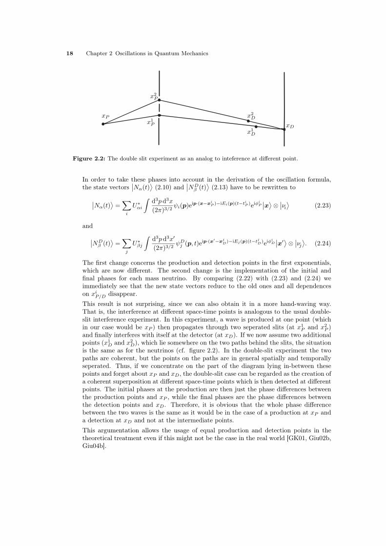
Figure 2.2: The double slit experiment as an analog to inteference at different point.

In order to take these phases into account in the derivation of the oscillation formula,the state vectors

∣∣Nα(t)⟩(2.10) and

∣∣NDβ (t)

⟩(2.13) have to be rewritten to

∣∣Nα(t)⟩

=∑i

U∗αi

∫d3pd3x

(2π)3/2ψi(p)eip·(x−xiP )−iEi(p)(t−tiP )eiφiP

∣∣x⟩⊗ ∣∣νi⟩ (2.23)

and∣∣NDβ (t)

⟩=∑j

U∗βj

∫d3p d3x′

(2π)3/2ψDj (p, t)eip·(x′−xjD)−iEj(p)(t−tjD)eiφiD

∣∣x′⟩⊗ ∣∣νj⟩. (2.24)

The first change concerns the production and detection points in the first exponentials,which are now different. The second change is the implementation of the initial andfinal phases for each mass neutrino. By comparing (2.22) with (2.23) and (2.24) weimmediately see that the new state vectors reduce to the old ones and all dependenceson xiP/D disappear.This result is not surprising, since we can also obtain it in a more hand-waving way.That is, the interference at different space-time points is analogous to the usual double-slit interference experiment. In this experiment, a wave is produced at one point (whichin our case would be xP ) then propagates through two seperated slits (at x1

P and x2P )

and finally interferes with itself at the detector (at xD). If we now assume two additionalpoints (x1

D and x2D), which lie somewhere on the two paths behind the slits, the situation

is the same as for the neutrinos (cf. figure 2.2). In the double-slit experiment the twopaths are coherent, but the points on the paths are in general spatially and temporallyseperated. Thus, if we concentrate on the part of the diagram lying in-between thesepoints and forget about xP and xD, the double-slit case can be regarded as the creation ofa coherent superposition at different space-time points which is then detected at differentpoints. The initial phases at the production are then just the phase differences betweenthe production points and xP , while the final phases are the phase differences betweenthe detection points and xD. Therefore, it is obvious that the whole phase differencebetween the two waves is the same as it would be in the case of a production at xP anda detection at xD and not at the intermediate points.This argumentation allows the usage of equal production and detection points in thetheoretical treatment even if this might not be the case in the real world [GK01, Giu02b,Giu04b].

2.4 Remarks on the Oscillation Formula 19

6. The last remark concerns a basic problem of the mixing of states as represented in(2.1), which is noted by some authors (e. g. [Zra98, Beu03]). That is, in non-relativisticquantum mechanics the superposition of states with different masses is forbidden due tothe Bargmann superselection rule [Bar54]. The usual argumentation is as follows: Non-relativistic quantum mechanics should be invariant under Galilean transformations. Ifsuch a transformation acts on a wave function—in the form of a transformation to anothersystem and then back to the original system—it results in a phase that depends on themass of the state. It then follows that the transformation of a superposition of differentmass states aquires a relative phase depending on the mass difference. This relative phasewould, in principle, be measurable. In order to avoid this problem, one usually imposea superselection rule, which simply forbids such superpositions. However, neutrinos arerelativistic and thus they are not described by the non-relativistic Schrödinger equationbut by the relativistic Dirac equation. Therefore, the invariance group is the Lorentzrather than the Galilean group. But, the action of a Lorentz transformation on a statevector that satisfies the Dirac equation does not yield a mass-dependend phase factorand hence no relative phase for a superposition will occur. Furthermore, it was shownthat the relative phase is just the non-relativistic residue of the usual twin paradox ofspecial relativity and thus there is no reason to wonder about its appearance [Gre01].

Chapter 3

Neutrinos as Plane Waves

In this chapter we will approximate the mass neutrinos as plane waves. The simple treatmentin the first section yields a probability which is not satisfactory from an experimental pointof view, because it contains an unmeasurable time-dependence. This will be changed in thesecond section, where different assumptions are used to convert the temporal into a spatialdependence. The discussion of these assumptions will be done in the third section. Finally,the last section contains a few remarks on the discussed plane-wave treatment.

3.1 The General Plane Wave Solution

As already mentioned in the previous chapter, the flavour neutrinos are described as superpo-sitions of mass neutrinos whose space-time and energy-momentum dependence are stored inwave functions ψi(p) =

⟨p|ψi

⟩. In this chapter these wave functions will be considered as plane

waves with definite momenta pi, or in other words, the∣∣ψi⟩ are be momentum eigenstates.

Hence, the wave functions in momentum space are given by delta functions

ψi(p) = δ(p− pi). (3.1)

Using the Fourier transform (2.11), then yields the wave functions in position space

ψi(x,xP , t, tP ) =1

(2π)3/2exp

[ipi · (x− xP )− iEi(t− tP )

], (3.2)

which are the mentioned plane waves. The dispersion relation for the energy Ei is the same asin (2.9), but this time the momentum has the definite value pi. Thus,

Ei =√p2i +m2

i . (3.3)

In order to derive the oscillation probability for the plane-wave treatment, we additionallyhave to fix the description of the detection process. Since plane waves do not have a spatialuncertainty, we will assume a point-like detection process, given by (2.14) and (2.15), here.That is, the detection shall take place at one well-defined space-time point (xD, tD). Underthis assumption the general probability (2.17) reduces to

P(α→ β;L, T ) =1

(2π)3

∑i

∣∣Uβi∣∣2∣∣U∗αi∣∣2+

2(2π)3

Re

[∑i<j

UβiU∗αiU

∗βjUαj exp

[i(pi − pj) ·L− i(Ei − Ej)T

]]. (3.4)

21

22 Chapter 3 Neutrinos as Plane Waves

This probability consists of two parts. The first part, which does not depend on spaceand time, is the transition probability which we would get if the superposition of the massneutrinos were incoherent. This would for example be the case if the flavour neutrinos werenot a superposition but a statistical mixture of mass neutrinos with probabilities given bythe PMNS-matrix. The second part is the actual oscillation part that includes the coherenteffects and therefore gives rise to oscillations. Since a real neutrino beam always has an energy-momentum spread, the second term will be washed out if the distance or time is large enoughand no oscillations can be measured in this region. However, even if this is the case, thetransition probability is not zero due to the incoherence term. A more precise estimation forthis will be given in the remarks at the end of this chapter. However, if the neutrino beam isdescribed by plane waves which do not have an energy-momentum spread, there will not occursuch effects in this treatment. This is the first hint on the incompleteness of the plane wavetreatment, which, in the end, leads to the necessity of using wave packets instead.Nevertheless, the probability (3.4) looks quite simple and it should be easy to calculate

some results for real experiments. But after a closer look, one sees that it lacks in two points.First, in real experiments no one measures the time between the production and detection of theneutrino. And in most cases, e. g. solar neutrinos, it is rather impossible to know the productiontime. Therefore, one has to convert the time dependence into a distance dependence, sincethis is usually known to a much higher accuracy. Second, the exponential in (3.4) contains theenergy and momentum of the different mass neutrinos. These are impossible to know, becausethe neutrinos cannot be measured directly. In particular, the only observed particles are theones that participate in the detection process, or the production process if it is observed. Thoseparticles are the corresponding leptons or nuclei to the neutrinos and have only one specificenergy and momentum. Thus, the energy and momentum of the mass neutrinos have to berewritten in terms of the measured momenta of the actually detected particles. These easylooking tasks give rise to a vast number of papers written by different authors who all claimdifferent ways to be the only right ones.

3.2 Time to Space Conversion

The rewriting of the oscillation probability (3.4) in an only space dependent way is not uniqueand in fact there are basically four different possibilities mentioned in the literature. They areusually called:

1. equal-energy assumption,

2. equal-momentum assumption,

3. equal-velocity assumption,

4. energy-momentum conservation.

In the following the main points in these assumptions will be summarized while the discussionof the different cases is postponed to the next section. For simplicity the derivations will bedone in only one spatial dimension. This is not a crude approximation since the neutrinostravel a macroscopic distance, which means a deviation from the one dimensional case wouldcause a separation of the mass neutrinos and thus no oscillation would be measurable. Afurther simplification will be the restriction to the argument of the exponential in (3.4), whichis the only interesting quantity here. In particular it will be denoted as

φ := (pi − pj)L− (Ei − Ej)T, (3.5)

3.2 Time to Space Conversion 23

and shall get an index E, p, v and c in the four different cases, respectively.

Equal-Energy Assumption This assumption is the easiest one. It was first mentionedby Lipkin in 1995 and then repeated and defended in several following papers [Lip95, GL97,Sto98, Lip99, Lip02, Lip06]. Equal energy means, all mass states are supposed to have thesame energy, that is, Ei = Ej = E. Then the time dependence of (3.5) simply vanishes andthe resulting argument can be written as

φE = (pi − pj)L =p2i − p2

j

pi + pjL =

m2j −m2

i

pi + pjL, (3.6)

where the last step requires the use of the dispersion relation (3.3). In order to get a relationin terms of the measured momentum, we can define an average momentum

p :=1Nm

∑i

pi. (3.7)

Since the difference of the momenta pi must be smaller than the momentum uncertainty of theflavour neutrino—as already mentioned in section 2.1—they have to be nearly equal and wecan approximate them by the average momentum. Thus, the argument becomes

φE ≈m2j −m2

i

2pL. (3.8)

If the neutrinos are considered to be relativistic (i. e., pi mi)—as they in fact are inpractice—the momenta can be expanded in terms of the mass

pi =√E2 −m2

i = p0 −m2i

2p0+O

(m4i

p30

), (3.9)

where p0 = E is the momentum and energy of a massless neutrino. Using this expansion torewrite p in terms of p0 changes the argument to

φE ≈m2j −m2

i

2p0L. (3.10)

The terms proprtional to m2i in (3.9) are neglected, which can be done if

m2j −m2

i

2p0

m2i

4p20

m2j −m2

i

2p0. (3.11)

The validity of this estimation can be seen from experimental details, since in usual experimentsonly neutrinos with an energy higher than about 100 keV can be detected, while the mass isfound to be smaller than about one eV (see [Giu04b] footnote 3 and references therein). Thus,m2i /p

20 . 10−10, which is obviously in good agreement with (3.11).

Equal-Momentum Assumption This is the oldest and most common assumption used innearly every publication on neutrino oscillations. Equal momentum means pi = pj = p. Thus,this time the space dependent term in (3.5) vanishes and the argument can be written as

φp = −(Ei − Ej)T = −E2i − E2

j

Ei + EjT =

m2j −m2

i

Ei + EjT. (3.12)


In the last step we again used the dispersion relation (3.3). With the same argumentation asin the equal-energy assumption we can introduce an average energy

E :=1Nm

∑i

Ei (3.13)

and rewrite the argument as

φp ≈m2j −m2

i

2ET. (3.14)

Now, in the same manner as in the previous assumption, the relativistic limit can be con-sidered. Here, the expansion of the energy in terms of the mass yields

Ei =√p2 +m2

i = p0 +m2i

2p0+O

(m4i

p30

), (3.15)

where p0 = p is the momentum and energy of a massless neutrino. Here, p0 rather than E0

is used in order to have a consequent notation in the different assumptions. This expansionsallows us to rewrite the average energy and thus the argument to

φp ≈m2j −m2

i

2p0T. (3.16)

The terms proportional to m2i in (3.15) are again neglected. This can be validated by the

same argument as in the equal-energy assumption. The last step is the conversion of thetemporal dependence into a spatial dependence. This can be done by using the classicalvelocity vi = p0/Ei, which is also the group velocity for a wave packet with mean momentump0. However, in principle, no such velocity is defined in the case of plane waves, which isagain a point against the usage of plane waves and for a description in terms of wave packets.Expanding the velocity in terms of the mass in the relativistic limit yields

L

T= vi =

p0

Ei= 1− m2

i

2p20

+O(m4i

p40

). (3.17)

We can again neglect the second term since it is smaller than ∼ 10−10 if the same argumentsas in the equal-energy case are used. This allows us to approximate T ≈ L and the final formof the argument is

φp ≈m2j −m2

i

2p0L, (3.18)

which is the same as the one in the equal-energy assumption.

Equal-Velocity Assumption The equal-velocity assumption deals—as suggested by thename—with the velocities of the mass neutrinos, in particular the group velocities, which is inthe same way insufficient as in the equal-momentum assumption. These velocities are assumedto be equal for all neutrinos:

vi =piEi

= v =L

T∀ i. (3.19)

3.2 Time to Space Conversion 25

The first mention of this assumption was independently made by Takeuchi et al. [TTTY99]and De Leo et al. [DLDR00]. The argumentation here is the one of Takeuchi et al.We can use (3.19) to rewrite the general argument (3.5). In order to do so we should note

that (3.19) implies EiT = piL/v2. Then the argument changes to

φv = (pi − pj)(

1− 1v2

)L

= (pj − pi)L

v2γ2, (3.20)

where we introduced the usual relativistic γ-factor γ = 1/√

1− v2. The factor also gives arelation between the momentum and mass: pi = γvmi. Inserting this in (3.20) after themomentum part is extended, yields

φv =p2j − p2

i

pi + pj

L

v2γ2

=m2j −m2

i

pi + pjL, (3.21)

which is the same as in the equal-energy assumption. Hence, we get the same result if we firstintroduce an average momentum and then go to the relativistic limit:

φv ≈m2j −m2

i

2pLpimi≈

m2j −m2

i

2p0L. (3.22)

Energy-Momentum Conservation In this approach, a rigorous treatment of the energyand momentum conservation in the production process of the neutrino is performed. This wasfirst done by Winter in 1981 [Win81] and then used by several other authors [Gol96, GK01,Giu01, Giu06] to show that neither the equal-energy assumption nor the equal-momentumassumption are satisfying.If the production process of the neutrino is a two-body decay, within the rest-frame of the

decaying particle, the energy-momentum conservation relation can be written as

EI =√p2i +M2 +

√p2i +m2

i . (3.23)

Here, EI is the energy of the decaying particle, pi is the momentum of the neutrino and therecoiling particle and m2

i and M2 are the neutrino and recoiling particle mass, respectively.Of course, the same considerations can be done for more complicated processes. We just haveto insert the energy of the entire initial state on the left-hand side and the entire mass andthe sum of the momenta of all recoiling particles on the right-hand side, while working in thecenter of mass system of the neutrino and the recoiling particles. This is the reason why theleft-hand side is called EI rather than just the mass of the decaying particle.From (3.23) we can find the value of the momentum pi:

pi =

√p2

0 −2(E2

I +M2)m2i −m4

i

4E2I

= p0 −E2I +M2

2E2I

m2i

2p0+O

(m4i

p30

), (3.24)


where again p0 = E2I−M

2

2EIis the momentum of a massless neutrino. The higher order terms

in this expansion can be neglected even in the case of relatively low neutrino energies. Forexample, a neutrino with mass 1 eV and momentum p0 ∼ 100 eV, which is not even observable[Giu04b], would give a correction of order 10−6, four orders less than the first correction term.Using the dispersion relation (3.3) yields the energy of the neutrino

Ei =√p2i +m2

i =

√p2

0 +2(E2

I −M2)m2i +m4

i

4E2I

= p0 +E2I −M2

2E2I

m2i

2p0+O

(m4i

p30

). (3.25)

In the notation of [GK01], the factors E2I +M2/2E2

I and E2I −M2/2E2

I are called ξ and 1− ξ,respectively. Since this simplifies the notation we will also use the factor ξ here. If we nowinsert (3.24) and (3.25) into the general argument (3.5) and neglect the higher order terms, weget the following argument for the energy-momentum conservation assumption:

φc ≈ ξm2j −m2

i

2p0L+ (1− ξ)

m2j −m2

i

2p0T. (3.26)

In order to get a relation between the time and distance, we can again compute the groupvelocity (where the question of the existence of this velocity is the same as in the other as-sumptions):

vi =piEi

= 1− ξ m2i

2p20

− (1− ξ)m2i

2p20

+O(m4i

p40

)= 1− m2

i

2p20

+O(m4i

p40

). (3.27)

Again the higher order terms can be neglected for relatively low neutrino energies. In particular,using the same example would give a correction of order 10−8 here.Inserting (3.27) into (3.26) then yields

φc ≈ ξm2j −m2

i

2p0L+ (1− ξ)

m2j −m2

i

2p0L

=m2j −m2

i

2p0L, (3.28)

where we also neglected the terms which come from the m2i terms in the velocity, because as

in the equal-energy assumption and the equal-momentum assumption the bound

m2j −m2

i

2p0

m2i

2p20

m2j −m2

i

2p0(3.29)

holds for realistic neutrinos.As can be seen from (3.28), the factor ξ does not show up in the final argument.

3.3 Discussion

There is an extensive discussion on the different options in the literature (see the citations inthis section) without reaching a consensus on any of those assumptions. We will present parts

3.3 Discussion 27

of the discussion in this section. In particular, the equal-energy assumption and the energy-momentum conservation are the most favoured ones. Beuthe [Beu03] gave a comprehensivesummary of the arguments used in the literature. In the following there will be some overlapwith his presentation but we will present some additional arguments.As can be seen from the last section, there is no difference in (3.10), (3.18), (3.22) and (3.28)

after the relativistic limit is applied. That is, the argument of the phase is for all cases

φ =m2j −m2

i

2p0L,

or by introducing the, so called, oscillation length Loscji = 4πp0/(m2j −m2

i )

φ = 2πL

Loscji.

This result is not surprising since the relativistic limit was applied by expanding the energyand momentum in terms of the mass and then neglecting all terms of second or higher orderin the mass. Hence, only terms that describe massless neutrinos are considered. But in themassless case all energies and momenta are the same: Ei = Ej = pi = pj = p0 and everydistinction in the assumptions simply vanishes. This means, in order to discuss the validity ofthe assumptions one cannot use the results obtained in the relativistic limit.A first look at the four assumptions shows that they are incompatible. For example, if the

neutrinos with different masses had the same energy they could not have the same momentumand vice versa. In particular, this means they also could not have the same velocities in thiscases. If energy-momentum conservation is assumed, (3.24) and (3.25) show that neither theenergy nor the momentum can be equal. Nevertheless, the equal-velocity assumption could, inprinciple, be used in this case.A closer look then shows that the plane wave treatment itself cannot be the last step. That

is, assuming a production process for a neutrino where all particles are described by planewaves. Then the energies and momenta of the non-neutrino particles are fixed and energy-momentum conservation determines the exact values for the neutrino. This is a missing massexperiment [Lip95] and allows only the production of a mass eigenstate. Hence, no oscillationswould occur. But, since oscillations are observed one has to improve the treatment. This willbe, as usual, the description in terms of wave packets which we will do in the next chapter.However, the plane-wave description already leads to the oscillation phase, which will be thesame in the wave-packet treatment. Therefore, we should first discuss the easier treatment ofplane waves before going over to wave packets. Nevertheless, in order to do so, we have toassume some results from the wave packets. In particular, these will be the uncertainties forenergy, momentum and position as well as the group velocities.A rough estimation of the uncertainties yields–as already noted in section 2.1

σE >∣∣E2 − E1

∣∣ and σp >∣∣p2 − p1

∣∣,to be necessary in order to allow oscillations.In the following, we will discuss the arguments for each of the assumptions seperately.

• The equal-energy assumption is the by far most discussed assumption. There are basicallythree different arguments given for using equal energies for the mass neutrinos.

First of all, in [Lip95, Lip99] the uncertainties in the production process are consideredand it is claimed that the energy uncertainty can be neglected compared to the momentum


uncertainty. The argument goes as follows: Assuming the initial particle, which decaysto the neutrino, to be at rest gives a momentum uncertainty from the localisation ofthe particle, which, in turn, gives an energy uncertainty σEI ∼ σ2

pI/mI . Since σEI isof second order in σpI , it is neglected. This is actually an over simplified view, becausethe produced neutrino is not at rest and thus the energy uncertainty is of first order inthe momentum uncertainty: σEν ∼ σpνpν/Eν ∼ σpν . Moreover, even if σEν σpν , theuncertainty does not have to be exactly zero.The second argument is given in [GL97, Lip99], where a boundary condition for theneutrino wave function is assumed. This is, the probability of finding a neutrino witha wrong flavour at the production point vanishes for all times. The boundary conditionthen leads to a factorization of the flavour and time dependence and, by Fourier transformof the time, to a factorization of flavour and energy. Therefore, only mass neutrinos withthe same energy can give rise to a flavour change. However, the authors did not give areal reason why the condition should be valid for all times. And moreover, in the wavepacket picture the packets leave the region of production rather quickly which then leadsto a vanishing probability and the condition becomes meaningless [Beu03].As a third argument a fuzziness in time is assumed [GL97, Lip99]. This comes fromthe spatial spread of the wave packets which results in a non-zero overlap time with thesource (or detector). Thus, one has to average the flavour-change probability over thisfuzzy arrival time. If the source (or detector) is stationary [Sto98, Lip02] this leads to awash out of all terms with different energies. This can already be seen in the plane wavepicture, where the average can be written as (cf. [Beu03, Giu06])∫

dtP ei(pi−pj)(xD−xP )−i(Ei−Ej)(tD−tP ) = 2π δ(Ei − Ej) ei(pi−pj)(xD−xP )−i(Ei−Ej)tD .

This is of course only true if the integration range is infinity, which can be assumed inthe case of stationarity. If this is not the case, the delta function becomes a narrow peakaround Ei − Ej . However, real processes are not stationary on the microscopic scale,because the particle that decays into the neutrino has an inherent energy uncertaintydue to its instability of the order 1/τ the inverse life-time. Likewise, the same is true forthe detection process.A further argument, which is against the assumption of equal energy, is the question ofLorentz invariance. It can be shown that the Lorentz transformation, from one frame toanother, of the energy and momentum leads to a non-vanishing difference in the energyeven if it is zero in one particular frame [Giu01].In conlusion, the arguments for the equal-energy assumption are not very convincing, butat least from the third argument it can be said that in the case of a nearly stationaryprocess the interference terms of the wave packet components with equal energies willgive the main contribution. However, this does not fix the energies to be exactly equal.

• The equal-momentum assumption is more or less the poor cousin in the discussion onwhich is the right assumption. On the one side it is used by almost all authors to cometo a quick solution for the probability, but on the other side no one gives arguments forthe correctness of this assumption. On the contrary, all given arguments predict thatit is wrong. These are, in principle, all arguments that are used for the equal-energyassumption. For example, if the uncertainty of the momentum is larger than the energyuncertainty there is no reason to assume the momenta to be equal. Moreover, the equalenergies in a nearly stationary process predict different momenta due to the differnet

3.3 Discussion 29

masses. In addition, the question of Lorentz invariance provides the same difficulty as inthe energy case. That is, the assumption of equal momenta is only valid in one particularframe [Giu01].

• The energy-momentum conservation assumption has the advantages of already contain-ing the conservation laws of energy and momentum and on the other hand being themost general assumption in the sense that neither the energy nor the momentum areconstrained. The missing of a constraint allows the usage of this assumption in anyLorentz frame. One just has to transform the factor ξ into the relevant frame. In fact,one can show that either ξ > 1/2 or ξ < 1/2 is valid in any system. In particular, thismeans that a system, where the energies are equal, cannot be transformed into a system,where the momenta are equal [Giu01], because equal energies correspond to ξ = 1 whileequal momenta correspond to ξ = 0.

The only real criticism on this assumption is made in [Beu03]. Therein, Beuthe claimsthat, for example, in the case of a pion decay at rest (π → µν), the energy-momentumuncertainty of the pion is much larger than the difference in masses m2

j −m2i and thus it

should be meaningless to compute the values of the neutrino energy and momentum toorder m2. However, this would also mean that it is meaningless to compute a oscillationprobability since the interference terms are of order m2

j −m2i . A more detailed analysis

of the uncertainties shows the following: From (3.24) and (3.25) the computation of theuncertainties of pi and Ei, under the assumption of a pion uncertainty σEI , yields

σpi ∼ σEi ∼M2m2

i

E2I p0

σEIEI

.

Since M/EI ∼ 1 for a pion decay it is obvious that the uncertainty for the neutrino canbe neglected—as long as σEI EI—for the computation of the oscillation phase.

• The last assumption to be discussed is the equal-velocity assumption. As already said, itcould only be used in the case of different energy and momenta. However, there is oneargument that makes it very unlikely to use this assumption. That is, equal velocitiesmeans equal γ-factors and hence (cf. [OT00])

EiEj

=pipj

=mi

mj.

Obviously, this can not be true for the equal energy and equal momentum case since thenalso the masses must be equal. But even in the case of different energies and momenta thisrelation cannot hold, because it is inherent Lorentz invariant and it was shown [Giu01]that one can always transform to a system where either the energies or the momentaare equal, which then, in turn, breaks the relation above. Therefore, the equal-velocityassumption can be ruled out.

In conclusion, the assumption of energy-momentum conservation seems to be the most sat-isfying one. On the one side it is the most general one that includes the conservation laws. Onthe other side, all the other assumptions lack in some point or are only approximately valid.However, it is possible that the equal-energy assumption or the equal-momentum assumptionare valid in some particular Lorentz frames, while the time average yields the energies to be,at least, nearly equal.


3.4 Remarks on the Plane Wave Treatment

The Wash-Out of the Oscillations As already mentioned in 3.1 the energy-momentumspread of a real neutrino beam leads to a wash out of the oscillations if the time or distancebetween production and detection is large enough. This can be seen in the following way: Theenergy-momentum spread requires an averaging of the probability over the spread. Hence,

P(α→ β;L, T ) =1

σ6pσ

2E

∫d3pid3pjdEidEjP(α→ σ;L, T ), (3.30)

where P is the averaged probability. In (3.4) the only part that depends on the energy andmomentum is the phase and the integration of this yields a term proprtional to (σ6

pσ2EL

2T 2)−1

which vanishes for large L and T . Thus, the result after the average is

P(α→ β;L, T ) =1

(2π)3

∑i

∣∣Uβi∣∣2∣∣U∗αi∣∣2,which can be non-zero even in the case of α 6= β.

The Factor of Two Problem Several authors showed that it is possible to get an oscillationphase that is two times the standard one [Lip95, SWS95a, SWS95b, WS96, DLDR00, DLNR04,DLNR03]. As it is pointed out in the replies to this problem [L+96, Kay97, BLSG99, GK01,Giu02b, OST03, Giu04b], the origin of the factor is the superposition of different mass states atdifferent times (or positions). In particular, if different energies or momenta are assumed, theneutrinos will have different group velocities and thus arrive at different times Ti = (Ei/pi)L(or positions Li = (pi/Ei)T ) at the detector. Then the phase difference is given by

φ = (pi − pj)L− (EiTi − EjTj) =m2j

pjL− m2

i

piL

or

φ = (piLi − pjLj)− (Ei − Ej)T =m2j

EjT − m2

i

EiT,

which in the case of equal momenta (or energies) yields an argument twice as large as thestandard ones (3.10), (3.18), (3.22) and (3.28). This result is general and can be obtained inall assumption schemes—except the equal-velocity assumption, where the arrival times are allthe same and the computation shown in section 3.2 then gives the standard result.However, the important point to explain this wrong result was given by [GK01]. That is, the

different waves must be coherent, which implies additional phases as we showed in section 2.4.If these phases are properly taken into account we obtain the standard result back.In section 2.4 we also showed that the use of the coherence condition gives a result which

is the same as if production and detection at the same space -time points is assumed. Thismeans, if we ignore the possibility of different production and detection points we can, in turn,state that the interference must be calculated at the same space-time point. This argumentwas used by [L+96, Kay97, BLSG99, OST03, Giu04b].

3.4 Remarks on the Plane Wave Treatment 31

Do Charged Leptons Oscillate? Closely related to the factor of two problem is the ques-tion whether the recoil particle, in for example the decay W± → l±σ + νσ, can oscillate. Theauthors of [SSW95, SWS95a, SWS95b, WS96] claimed that this oscillations should appearfor recoil leptons—or, for example Λs, in the case of kaon oscillation. As pointed out by[DMOS97, BLSG99] this effect actually bases on the assumption of superpositions at differenttimes. Thus, the argumentation on the correctness of these oscillations is the same as in thefactor of two case. The calculation particularly reduces to the standard case with no oscillationsif the superposition is calculated at the same space-time point. Moreover, in [GK01, Giu04b]it is argued that oscillations in the probability of finding a charged particle are, in principle,impossible, because this would violate the conservation of the probability. However, the mixingmatrix in (1.16) can be considered to act on the leptons rather than the neutrinos. Then themass leptons are different from the flavour leptons and oscillations could occur. But since themasses of the leptons differ from around 500 keV to 2GeV very high energies which exceed afew hundred TeV and some new physics in order to detect such a flavour superposition areneeded to get this effect [Akh07].

Chapter 4

The Intermediate Wave Packet Model

4.1 The Uncertainties of a Neutrino

In the previous chapter the description of the neutrinos was done in the plane-wave approxi-mation, although the arguments in the discussion often relied on a wave-packet interpretation.This already shows the insufficiency of regarding neutrinos as plane waves. A more importantreason why one has to use wave packets instead comes from the experimental conditions. Inparticular, neutrino-oscillation experiments are localised in space and the important measure-ment is the distance between production and detection. This is contrary to usual high-energyphysics experiments, where one is more interested in the energies and momenta of the parti-cles. Thus, the usual plane-wave approximation cannot hold for neutrinos. Moreover, as willpresented shortly, a too precise measurement of energy and momentum destroys the oscillationbehaviour.Even though the plane-wave and wave-packet approach seems to be quite different, there is

an interesting feature that should be noted. In 1996, Kiers, Nussinov and Weiss [KNW96]showed that it is impossible to perform an experiment which can discriminate between anensemble of wave packets with equal mean energy E and energy spread σE and an ensemble ofplane waves, whose definite energies are distributed around E with the same spread ∆E = σE .However, before the wave-packet treatment will be described some comments on the involved

uncertainties shall be made. Since this is done in detail in [KP93, GK07] only a summary ofthe important points will be given here.The first who considered the effects of wave packets on neutrino oscillations was Nussinov

in 1976 [Nus76] who used simple physical arguments in order to estimate a size of the packets.From the separation of the packets due to their different velocities, he could then predict acoherence length, which describes the maximal distance in which oscillation can occur. Twentyyears later, he together with Kiers and Weiss [KNW96, KW98] showed, that the coherenceof the different mass neutrinos could be restored, even if they are spatially separated, by takinginto account the temporal resolution of the detection process. This was already noted whenthe interference at different space-time points was discussed in section 2.4.In 1981 Kayser [Kay81] studied the influence of the uncertainties on neutrino oscillations.

In particular, he showed, that the energy or momentum uncertainties, σE or σp, for the neutrinobecome smaller than the energy or momentum difference of the corresponding mass neutrinos,|Ei − Ej | or |pi − pj |, by for example more precise measurements on the initial and recoilparticles of the production. Under this assumption, on the one hand one precisely knows whichmass neutrino is produced and on the other hand the induced spatial uncertainty σx ∼ 1/σEor σx ∼ 1/σp becomes larger than the oscillation length, which leads to a wash out of the

33

34 Chapter 4 The Intermediate Wave Packet Model

oscillations.Therefore, the requirements for oscillations to occur can be summarised (for relativistic

neutrinos) as follows:

1σE∼ 1σp∼ σx < Losc ∼

1∣∣Ei − Ej∣∣ ∼ 1∣∣pi − pj∣∣ . (4.1)

In the following we will give an estimation of the wave-packet size for the general case andparticularly for the muon decay (the more detailed description can be found in [GK07] p. 311ff).There are basically two different mechanisms influencing the size of the wave packet. Theydepend on the physical situation.

Natural Linewidth If the neutrino is produced in a decay of a free particle, the importantinfluence on the wave-packet size comes from the mean life time of the decaying particle. Thatis, the emission of a coherent wave train will be interrupted due to the decay of the particle.Therefore, the maximum size of the wave packet—for a relativistic neutrino—can be estimatedto

σx ∼ τX ,

where τX is the mean life time of the decaying particle X. This is valid in the rest frame ofthe decaying particle. If it decays in flight, the relativistic time dilation changes the size of thewave packet to

σx ∼ γτX ,

where the usual γ-factor was included. This factor is given by γ = EX/mX , the ratio of theenergy and mass of the decaying particle.For the muon decay

µ+ −→ e+ + νe + νµ

at rest we can estimate the size of the wave packet to

σx ∼ τµ ∼ 2.2 · 10−6s ∼ 103m ∼ 1010eV−1.

The corresponding momentum uncertainty is then

σp ∼1σx∼ 10−10eV.

Collision Broadening If the neutrino is produced in a decay of a particle contained in amedium, there are more effects that influence the size of the wave packet. In particular, theemission of a coherent wave train will be interrupted if one of the involved particles collideswith a particle of the medium. Thus, the important time scale is the average time betweentwo collisions:

τ ∼ minX

[`XvX

],

where `X is the mean free path of particle X and vX its velocity. X can be any of the involvedparticles without the neutrinos, because they are relativistic and leave the region as soon as

4.2 Gaussian Wave Packets 35

they are produced. The velocities can be estimated for the initial particles by the mean thermalvelocity and for the produced particles by the kinematics of the process. The mean free pathis a bit more complicated. It is defined as

`X =1

πb2N,

where N is the particle number density of the medium and b the impact parameter for theCoulomb scattering with the electric field of the nuclei, which can be written as

b ≈ 4παZT

.

Here, α is the fine-structure constant, T the kinetic energy and Z the atomic number of thenuclei in the medium. There is, however, an upper bound for the impact parameter. Thatis, it cannot exceed half the mean internuclear distance, which can be estimated by 1/N1/3.Therefore, ` cannot be smaller than ∼ 1/N1/3.For a muon that decays in graphite at 300K. The values are Z = 6 and N ≈ 1023cm−3.

Then the internuclear distance is 1/N1/3 ≈ 2 ·10−8cm and the kinetic energy is T ≈ 4 ·10−2eV.From this we get a mean free path of `µ ≈ 5 · 10−17cm, which is smaller than the internucleardistance. Therefore, the value for the mean free path is given by the internuclear distance. Thevelocity of the muon is vµ =

√2T/mµ ∼ 2 · 10−5. Thus, σx ∼ 10−3cm. The mean free path of

the positron is the internuclear distance since it is annihilated as soon as it meets an electron.The velocity can be assumed to be ∼ 1 since it is relativistic. Thus σx ∼ `e ∼ 2 · 10−8cm.Which is smaller than the muon contribution. Therefore, for the neutrino we can estimatedσx ∼ 2 · 10−8cm and σp ∼ 2 · 103eV.

There is an important difference between the uncertainties and the production and detectionat different space-time points. That is, if all waves are produced at the same space-time pointthey will have a spatial uncertainty due to the localisation of the production process and themomentum uncertainty involved in this process. After they travelled to the detector, theywill be detected at one specific space-time point. But since the detection process also involvessome spatial and temporal uncertainties due to the localisation and finite detection time, thisdetection can in principle take place everywhere inside these uncertainties. Therefore, thedetector has to be described as a wave packet and the probability is the overlap integral overthe wave packet and the detector. On the other side, if production and detection at differentspace-time points are considered, this does not influence the shape of the wave packets neitherat the detector nor at the source and only effects the phases. But the phases have to satisfythe coherence condition which means they can be regarded as produced at some point anddetected at some other specific point

4.2 Gaussian Wave Packets

In this section we will review the calculation of the flavour changing probability for the caseof Gaussian wave packets. This was first done in 1991 by Giunti, Kim and Lee [GKL91] (asummary of this paper can be found in [KP93]) and extended by Giunti and Kim in 1997[GK98], where they took into account the spatial coherence width of the detection process.Finally, in 2002 Giunti [Giu02b] also included the temporal coherence width of the detectionprocess. Moreover, a summary of the whole calculation in three spatial dimensions can befound in [GK07].


Since we already introduced the most general treatment in chapter 2, we can directly calcu-late the version of [Giu02b] just by fixing the wave functions ψi(x,xP , t, tP ) for the propagatingmass neutrinos and the functions ψDi (x,xD, t, tD) for the detection process. As the title ofthis section implies, we will describe the mass neutrinos as Gaussian wave packets. Thus, wecan use the following momentum space wave function

ψi(p) =1

(2πσ2pP )3/4

exp(− (p− pi)2

4σ2pP

), (4.2)

where σpP is the momentum width of the packet coming from the uncertainty of the productionprocess and pi is the mean momentum of the wave packet. The factor in front of the exponentialnormalises the packet to ∫

d3p∣∣ψi(p)

∣∣2 = 1. (4.3)

Nevertheless, we will forget about the normalisation factors in the following calculation. But,however, we will come back to this question in the final result for the probability, which willthen be normalised to (2.18).The next step is to Fourier transform the momentum space function (4.2) into the position

space. Therefore, we use (2.11) which yields

ψi(x,xP , t, tP ) =∫

d3p

(2π)3/2ψi(p)eip·(x−xP )−iE(p)(t−tP )

=1

(2πσ2xP )3/4

exp[ipi · (x− xP )− iEi(t− tP )

]· exp

(−[(x− xP )− vi(t− tP )

]24σ2

xP

)(4.4)

In order to get this analytical result, we expanded the energy Ei(p) around the mean momen-tum pi. Thus,

E(p) = Ei + (p− pi) · vi with Ei =√p2i +m2

i , vi =piEi, (4.5)

where vi is the group velocity of the wave packet. It is important to note that the neglectionof higher order terms in the expansion also means a neglection of the spreading of the wavepacket. This can be done for relativistic neutrinos. The new width σxP introduced in (4.4) isthe spatial wave packet width, which is related to the momentum width by

σxP σpP =12. (4.6)

The integral in (4.4) and most of the following integrals are Gaussian. Therefore, they canbe calculated analytically.Before we can actually calculate the amplitude (2.16), we have to find an explicit form for

the wave function that describes the detection process. In order to get an analytical result weuse a Gaussian wave packet which shall be localised around the detection point xD with thespatial and temporal widths σxD and σtD , respectively:

ψDi (x,xD, t, tD) ∝ exp[ipi · (x− xD)− iEi(t− tD)

]exp

(− (x− xD)2

4σ2xD

− (t− tD)2

4σ2tD

). (4.7)


The mean energy and momentum of the detection process are the same as those of the propagat-ing mass neutrino. This is necessary, because the incoming mass neutrino excites the degreeof freedom of the detection process which corresponds to its mean energy and momentum[Giu02b].Now, we have everything together in order to calculate the amplitude (2.16). That is,

A(α→ β;L, T ) ∝∑i

UβiU∗αi

∫dt∫

dx

· exp[−ipi · (x− xD) + iEi(t− tD)

]exp

(− (x− xD)2

4σ2xD

− (t− tD)2

4σ2tD

)

· exp[ipi · (x− xP )− iEi(t− tP )

]exp

(−[(x− xP )− vi(t− tP )

]24σ2

xP

)

∝∑i

UβiU∗αi exp

(ipi ·L− iEiT

)exp

(−(L− viT

)24σ2

xi

), (4.8)

where for simplicity a new width σxi was introduced. It is related to the other widths by

σ2xi := σ2

xP + σ2xD + v2

iσ2tD . (4.9)

Result (4.8) shows that each mass neutrino is detected in a space-time region of width σxiaround the space-time point (L, T ). The size of this region is determined by the width of thepropagating wave packet and the spatial and temporal coherence widths of the detection pro-cess. The dominating contribution comes obviously from the largest of these widths. However,since we already assumed relativistic neutrinos in order to neglect the wave packet spreading,we can use this assumption again and approximate

σ2xi ≈ σ

2xP + σ2

xD + σ2tD = σ2

x. (4.10)

From the amplitude (4.8) we can now derive the probability for the flavour change by takingthe absolute square. Hence,

P(α→ β;L, T ) ∝∑i,j

UβiU∗αiU

∗βjUαj exp

[i(pi − pj) ·L− i(Ei − Ej)T

]

· exp

(−(L− viT

)24σ2

x

−(L− vjT

)24σ2

x

). (4.11)

This probability contains the same problem as the one for the plane-wave treatment (3.4).That is, we need to know the time interval between the production and detection processes inorder to really calculate P(α→ β;L, T ), but as we said in chapter 3.1 the time is not measuredin usual neutrino oscillation experiments. Therefore, we have to dispose the time dependence.In the plane-wave treatment this was done by using different assumptions which then allow aconversion of the time into a distance dependence. However, for the wave-packet treatmentwe cannot use this assumptions, because they rely on well-defined energies and momenta forthe mass neutrinos, which are not given for a wave packet that has inherent uncertainties.Therefore, we have to use another possibility, which will be the average over the time interval


T . Performing the corresponding integral, which is again Gaussian, yields

P (α→ β;L) ∝∫

dT P (α→ β;L, T )

∝∑i,j

UβiU∗αiU

∗βjUαj exp

(i(pi − pj) ·L− i(Ei − Ej)

vi + vjv2i + v2

j

·L)

· exp

(− (Ei − Ej)2σ2

x

v2i + v2

j

− L2

2σ2x

+(vi ·L)2 + (vj ·L)2

2σ2x(v2

i + v2j )

−[(vi − vj) ·L

]24σ2

x(v2i + v2

j )

).

(4.12)

In order to get a simplified expression we expand the mean momentum pi in powers ofm2i . This is the same as we have done in the energy-momentum conservation assumption in

chapter 3.2, but now we will use the more general ansatz in three spatial dimensions. Thus,

pi ≈ p0 − ξm2i

2p0with

ξ

2p0= − ∂pi

∂m2i

∣∣∣∣mi=0

, (4.13)

where p0 is the vector and p0 the absolute value of the momentum of a massless neutrino.While ξ is the three dimensional generalisation of the factor ξ introduced in chapter 3.2. Thehigher order terms can be neglected, because we will only consider relativistic neutrinos here.The same will be done in all following expression.Using the dispersion relation Ei =

√p2i +m2

i yields the expression

Ei ≈ p0 +(

1− p0 · ξp0

)m2i

2p0(4.14)

for the mean energy of the ith mass neutrino. The last quantity that we will approximate isthe mean velocity, which is given by the ratio of the mean momentum and energy. Hence,

vi ≈p0

p0−[p0

p0

(1− p0 · ξ

p0

)+ ξ]m2i

2p20

. (4.15)

Now we can insert these approximations into the probability (4.12) and neglect all appearingterms of higher than second order in m2

i . The resulting probability for relativistic neutrinos is

P (α→ β;L) =∑ij

UβiU∗αiU

∗βjUαj exp

[−2πi

L

Loscij− 2π2

(1− L · ξ

L

)2(σxLoscij

)2

−(

L

Lcohij

)2]

(4.16)

with the oscillation and coherence lengths

Loscij =4πp0

m2i −m2

j

and Lcohij =4√

2p20

m2i −m2

j

σx. (4.17)

Throughout the whole calculation we did not care about the factors in front of the exponen-tial. This will be changed now. The normalisation condition (2.18) can easily be applied on(4.16). If we for example take the sum over α, we can use the unitarity of the PMNS-matrixand the fact that all terms in the exponential vanish if i = j and get as a result just 1. Thismeans, the probability is already normalised, which allows us to use the equal sign in (4.16)rather than the proportional sign.In the following we will explain the physical meaning of the three exponential factors in the

probability.


The phase factor

exp[−2πi

L

Loscij

](4.18)

This factor describes the actual oscillations. As can be seen from chapter 3, it is exactly thesame as in the plane-wave treatment.

The localisation term

exp

[−2π2

(1− L · ξ

L

)2(σxLoscij

)2]

(4.19)

This term suppresses the oscillations if σx Loscji . This means, in order to get oscillations theproduction and detection process must be localised in a region much smaller than the oscillationlength. This is the reason why it is called localisation term. Since in usual experiments thiscondition is very well satisfied, we can ignore the this term and only use the effective probability

P (α→ β;L) =∑ij

UβiU∗αiU

∗βjUαj exp

[−2πi

L

Loscij−(

L

Lcohij

)2]. (4.20)

The coherence term

exp

[−(

L

Lcohij

)2]

(4.21)

This term suppresses the oscillations if the distance L becomes larger than the coherence length,that is L Lcohij . As could be seen in the detailed calculation of the probability, the coherenceterm basically comes from the last term in (4.12), which becomes large if the velocity of thewave packets is different. Therefore, this term describes the suppression of the oscillationsdue to the separation of the wave packets for different mass neutrinos. If the packets are toomuch separated they cannot have an overlap with the detection process and thus they cannotbe detected coherently. In this case the coherence term yields an effective flavour changingprobability, which is simply the probability for an incoherent mixing

P (α→ β;L) =∑i

∣∣Uβi∣∣2∣∣U∗αi∣∣2. (4.22)

If L Lcohij , the coherence is satisfied and the effective probability reduces to the one alreadyobtained in the plane-wave picture

P (α→ β;L) =∑i

∣∣Uβi∣∣2∣∣U∗αi∣∣2 + 2Re

[∑i<j

UβiU∗αiU

∗βjUαj exp

(2πi

L

Loscji

)]. (4.23)

Chapter 5

The External Wave Packet Model

During the last 20 years a number of models to describe neutrinos in QFT have been published.According to Beuthe [Beu03, Beu02] all these models can be grouped into four differentcategories: the external wave-packet models, the stationary boundary-conditions models, thesource-propagator models and the Blasone-Vitiello models. Since the last category of modelsuses a different approach than the other models, we will postpone its discussion to chapter 8.The source-propagator models proposed by Srivastava, Widom and Sassaroli [SWS98],where the neutrino is described by its propagator, which is coupled to a source but not to adetector, leads to non-standard oscillation lengths or oscillations of the recoil particle. Thereason is the same as in chapter 3.4 where the factor of two problem and the oscillation of recoilparticles was discussed. Since we ruled out these result, we will not discuss the QFT version ofit here. The stationary boundary-conditions models describe the neutrino as an internal particleproduced in a certain process which then propagates and is detected in another certain process.The important boundary condition assumed in these models is the stationarity of the sourceand the detector. This condition leads to a unique value for the energy of the neutrinos. Thebest examples of this kind of models are given by Grimus and Stockinger [GS96] as well asCardall and Chung [CC99]. As was shown by Beuthe [Beu03, Beu02], these models areactually special cases of the general external wave-packet model. Therefore, we will also notdescribe them here. The last category is the external wave-packet model whose first versionfor neutrinos was proposed by Giunti, Kim, Lee and Lee [GKLL93] and then a few yearslater generalised by Giunti, Kim and Lee [GKL98]. In this model they used Gaussian wavepackets for the external particles and described the neutrino by its propagator. Similar modelswere used by Kiers and Weiss who replaced the external wave packets by quantum oscillators[KW98] and by Cardall who pays more attention on the spin structure [Car00]. The mostgeneral version of this kind of models was given by Beuthe [Beu03, Beu02]. In this chapter wewill review his computation of the neutrino oscillation formula. The whole calculation involvesquite a lot of steps, which are given in great detail in [Beu03]. Therefore, we only present themain steps and arguments here. To be consistent with the original computation we have tochange some of our notations, but this will be explicitly noted when it is important.

5.1 The Jacob-Sachs Model

The first authors who used a model in line with the external wave-packet model were Jacoband Sachs. They used it to describe the propagation of unstable particles in QFT [JS61].A few years later Sachs applied the model to Kaons in order to describe their oscillations

41

42 Chapter 5 The External Wave Packet Model

x x′

xP xD

PI(q)

PF (k)

DI(q′)

DF (k′)

L, T

Figure 5.1: Propagation of the neutrino between the source and the detector centered aroundxP and xD, respectively (reproduced according to [Beu03]).

[Sac63]. In the following section we will describe this model and how it can be applied to thedescription of neutrino oscillations.

The Feynman Diagram The basic point in the external wave-packet model is that theneutrino is not considered as an observable particle, which is produced and/or detected, butthe whole process starting from the particle which produces the neutrino up to the particleswhich are produced in the neutrino detection is consider as on quantum field theory process.This description avoids the problem that we cannot regard the neutrino as an asymptoticallyparticle. Of course, we have to assume that the external particles for the overall process canbe considered as asymptotically free. In figure 5.1 we have depicted the situation. We considerthe production process PI → PF + ν and the detection process ν +DI → DF , where P and Dsymbolises all particles involved in these processes. The 4-momenta of the external particlesare q, k, q′ and k′, respectively. If we assume the production and detection to take place atxP = (tP ,xP ) and xD = (tD,xD) we can have the actual interaction points at x = (t,x)and x′ = (t′,x′), which lie somewhere inside the production and detection regions depicted ascircles around xP and xD. These, regions appear, because we assume the external particlesto be described as wave packets. The neutrino is then a internal particle that propagates themacroscopically distance L in the time T . Note that we can consider the diagram as a Feynmandiagram if we remove the circles.

The Wave Packets Before we go on with this analogy we will briefly introduce the notationfor the wave packets, which we will use in the following. The notation and normalisation followsroughly the one used in [PS95]. That is, the state vector which describes a particle with massm is given as the wave packet ∣∣ψ⟩ :=

∫[d3k]ψ(k)

∣∣k⟩,where [d3q] is the integration measure given by

[d3k] :=d3k

(2π)3√

2E(k),

with E(k) =√k2 +m2. Note that there is no time-dependence for the state vector |ψ〉. This

follows from the fact that we work in the interaction picture, where the time-dependence of themomentum eigenvector |k〉 is given by a phase exp(iE(p)t), while the momentum space wavefunction ψ(k) evolves in time due to a phase factor exp(−iE(p)t). Thus, both dependencies

5.1 The Jacob-Sachs Model 43

cancel each other. However, if we want to calculate the configuration space wave function bymeans of a Fourier transformation we have to take the time dependence into account.Furthermore, we will denote a momentum wave function which is sharply peaked and sym-

metric around K by ψ(k,K). The corresponding configuration space wave function is thencentered around the spatial origin. By means of the space-time translation operator exp(iP ·x0)we can shift this the maximum to x0 and time t0. The corresponding momentum space wavefunction is then denoted by

Ψ(k,K,x0, t0) := ψ(k,K)eiE(k)t0−ikx0 .

The Fourier transformation of this wave function then gives the configuration space wavefunction

Ψ(x, t,x0, t0) =∫

d3k

(2π)3ψ(k,K)e−iE(k)(t−t0)+ik(x−x0). (5.1)

For simplicity we will assume that the external particles PI , PF , DI and DF only consists ofone particle whose corresponding state vectors are given as∣∣PI⟩ :=

∫[d3q]ΨPI (q,Q,xP , tP )

∣∣PI(q)⟩,∣∣PF ⟩ :=

∫[d3k]ΨPF (k,K,xP , tP )

∣∣PF (k)⟩,∣∣DI

⟩:=∫

[d3q′]ΨDI (q′,Q′,xD, tD)

∣∣DI(q′)⟩,∣∣DF

⟩:=∫

[d3k′]ΨDF (k′,K′,xD, tD)∣∣DF (k′)

⟩,

The Amplitude As we mentioned before, we will interpret the process shown in figure 5.1as a Feynman diagram with an additional folding with the initial and final particles’ wavefunction. In turn this means we can compute the amplitude for the whole process of neutrinoproduction, propagation and detection by using the usual QFT rules for such diagrams. Forsimplicity we will consider the neutrino as a scalar particle and ignore the spin structure. Thiscan be done because we can factorise the spin part from the rest of the amplitude. In order to“proove” this we have to distinguish between three different possibilities [Beu03]:

1. If the neutrinos are relativistic their chirality and helicity is the same as we already notedin chapter 1.2. Since the weak interactions involve only left-handed neutrinos we knowthat only this helicity eigenstates propagate. Thus, we can factorise the spin structurefrom the amplitude, which can then be evaluated as if the neutrinos were scalars, i. e.

Aspin = H(s)Ascalar

where H(s) includes all spin relevant factors.

2. If the neutrinos are non-relativistic but have nearly degenerated masses, the spin structurefor the different helicities is nearly the same and we can again take the spin part out ofthe sum over the mass eigenstates∑

i

UβiAspini Uiα ∼

(∑s

H(s))∑

i

UβiAscalari Uiα.


3. If the neutrinos are non-relativistic with very different masses we cannot factorise theamplitude. However, the case of very different masses is not relevant for NO because thissituation corresponds to an incoherent mixing of the mass neutrinos and not a coherentone which is necessary for oscillations. However, even if an experiment can produce acoherent mixing for this case, the energy and momentum uncertainties would average outthe oscillation effect quite rapidly.

Thus, in conclusion we can neglect the spin structure in all cases relevant for oscillations.Now we can come back to the diagram in figure 5.1. Using the common Feynman rules yields

the amplitude

A(α→ β;L, T ) =⟨DF , DI

∣∣T[exp(−i∫

d4xHI)]− 1∣∣PI , PF ⟩, (5.2)

where HI is the interaction Hamiltonian, T is the time-ordering operator and we includedthe 1 to avoid the calculation of the trivial process, because in that case no neutrino wouldpropagate. For the explicit calculation of the amplitude we expand the exponential to secondorder in the coupling constant in HI , which yields

A(α→ β;L, T ) =∫

[d3q]ΨPI

∫[d3k]Ψ∗PF

∫[d3q′]ΨDI

∫[d3k′]Ψ∗DFAplane(q, k, q′, k′) (5.3)

where Aplane is the amplitude if all external particles were plane waves:

Aplane(q, k, q′, k′) =∫

d4xMP (q, k)e−i(q−k)x

∫d4x′MD(q′, k′)e−i(q′−k′)x′

G(x′ − x). (5.4)

HereMP (q, k) andMD(q′, k′) are the amplitudes for the interactions at the production anddetection vertex, respectively. The propagator for the neutrino is a bit more complicated. Sincethe neutrinos which interacts at x and x′ are flavour neutrinos we cannot just write down thepropagator as in the case of a mass neutrino. However, by definition we have

Gβα(x′ − x) :=⟨0∣∣T(νβ(x′)ν∗α(x)

)∣∣0⟩, (5.5)

which is the time-ordered two-point function. If we now insert the mixing of the field operators

να =∑i

Uαiνi, (5.6)

we obtain

Gβα(x′ − x) =∑ij

Uβi⟨0∣∣T(νi(x′)ν∗j (x)

)∣∣0⟩U∗jα=∑i

UβiGiiU∗iα, (5.7)

with the diagonal propagator for the mass neutrinos

Gii(x′ − x) =∫

d4p

(2π)4e−ip(x′−x) i

p2 −m2i + iε

=∫

d4p

(2π)4e−ip(x′−x)Gii(p2). (5.8)

5.2 External Particles as Gaussian Wave Packets 45

We assume that the renormalisation has been carried out and thus mi is the physical mass ofthe neutrino νi. After a shift in the variables x and x′ we finally obtain the amplitude

A(α→ β;L, T ) =∑i

UβiAi(i→ i;L, T )U∗iα

=∫

d4p

(2π)4ψ(p0,p)Gii(p2)e−iE(p)T+ipL, (5.9)

where ψ(p0,p) is the overlap function that describes the overlap of the wave packets both atthe source and the detector. It is given by

ψ(p0,p) =∫

d4xeipx

∫d4x′e−ipx′

∫[d3q]ψPI (q,Q)e−iqx

∫[d3k]ψ∗PF (k,K)eikx

·∫

[d3q′]ψDI (q′,Q′)e−iq′x′

∫[d3k′]ψ∗DF (k′,K′)eik′x′

MP (q, k)MD(q′, k′). (5.10)

Thus, the final amplitude A(α→ β;L, T ) is the sum of the amplitudes Ai(i→ i;L, T ), wherethe internal particle is a mass neutrino weighted by the mixing matrix elements UβiU∗iα.

5.2 External Particles as Gaussian Wave Packets

The crucial step in the actual calculation of (5.9) are the integrations within the overlapfunction. In most cases it is not possible to do this analytically. One exception is the assumptionof plane waves for the external particles. But this is spoiled by the same problems as in thequantum mechanical plane wave approximation. Another possibility is the assumption ofGaussian wave packets for the external particles. This is the approach done first in [GKLL93]and later in [Beu03]. As we already said we will not describe details here. The whole calculationcan be found in [Beu03].

Gaussian Wave Packets A Gaussian wave packet in the normalisation of [Beu03] is givenas

ψχ(p,pχ) =(

2πσ2pχ

)3/4

exp(−

(p− pχ)2

4σ2pχ

). (5.11)

By using (5.1) we find the configuration space version of it if we expand the energy to secondorder around the mean momentum pχ

E(p) ' Eχ + vχ · (p− pχ) +1

2Eχ

((p− pχ)2 −

(vχ · (p− pχ)

)2) (5.12)

with Eχ =√p2χ +m2

χ and vχ = pχ/Eχ. The Fourier transformation then yields

ψχ(x, t,pχ) =(2πσ2

xχ)−3/4

√det Σ

exp(−iEχt+ ipχx−

(x− vχt)Σ−1(x− vχt)4σ2

xχ

)(5.13)

with

σxχσpχ =12

and Σij = δij + (δij − vivj)2itσ2

pχ

Eχ. (5.14)


The matrix Σ is important because it detemines the spreading of the wave packet. As can beshown this spreading is different for the directions transverse and along vχ. In particular, thetransverse spreading begins at t ' Eχ/2σ2

pχ , whereas the longitudinal spreading begins at thelater time t ' E3

χ/2m2χσ

2pχ . This will become important later.

For the external wave packets we will neglect the spreading. Additionally, we assume that thefactorsMP (q, k) andM(q′, k′) vary only slowly over the width of the wave packets. Therefore,we can approximate them by their value at the mean momentum of the wave packets and thentake them out of the integrals in the overlap function. Moreover, we can take them out ofthe sum over the different mass eigenstates, because we suppose the neutrinos to be eitherrelativistic or having nearly degenerate masses, which results in the same factor for all massneutrinos.The different integrals in the overlap function can now be calculated. Finally we arrive at

ψ(p0,p) ∼ ψP (p0,p)ψ∗D(p0,p) (5.15)

with

ψP/D(p0,p) ∼ exp

[−

(p− pP/D)2

4σ2pP/D

−(p0 − EP/D − (p− pP/D) · vP/D

)24σ2

EP/D

](5.16)

The new energy and momentum variables are

pP := Q−K, EP := EPI − EPF ,pP := K′ −Q′, ED := EDF − EDI .

The explicit form of the uncertainties and velocities shall not be of interest to us at thispoint. However, they can be interpreted as the momentum and energy uncertainties as wellas the velocities of the source and detector, respectively. Since the propagation distance ismacroscopically for neutrino oscillations, the production and detection processes have to satisfyglobal energy-momentum conservation laws. Therefore, we can impose the conditions

pP = pD = p0 and EP = ED = E0. (5.17)

5.3 Three Different Amplitudes

The Pole Integration In the last section we found an expression for the overlap function.Thus, the last step in the computation of the amplitude is the momentum integral (5.9). Wewill do this integration in two steps, first we integrate over p0 to get rid of the poles in thepropagator and then we do the p integration.The integration over p0 involves a careful choice of the integration contour, because the

overlap function diverges at infinity in the complex plane. Since we will not go into detail,we just mention that we can perform the integration by using the Jacob-Sachs theorem (cf.[Beu03] appendix A). This theorem states that the integral has for T → ∞ the asymptoticalbehaviour ∫

dp0ψ(p0,p)G(p2)e−ip0T → π

E(p)ψ(E(p),p)e−iE(p)T . (5.18)

Thus, the remaining part of the amplitude is given by

Ai ∼∫

d3p

Ei(p)ψ(E(p),p)e−iE(p)T+ipL, (5.19)

5.3 Three Different Amplitudes 47

which can be seen as an amplitude in the intermediate wave packet model. The overlap functionwould then be the wave function for the ith mass neutrino. Hence, we can interpret the processin figure 5.1 as the production of a neutrino as a superposition of wave packets one for eachmass neutrino, which are then detected. Nevertheless, there is an important difference to thismodel. That is, the overlap function contains the information on the source as well as thedetector which spoils the causality. This point was discussed in detail by Giunti [Giu02a]who showed by using a different ansatz that the produced wave packets are only functions ofψP (p0,p). The phase factor then comes from the propagation and the detection process finallyleads to the remaining function ψ∗D(p0,p).

The 3-Momentum Integrations Unfortunetaly, the last integration over the 3-momentumcannot be done analytically. But according to the form of the integrand we have two possibilitiesfor an approximation:

1. Laplace’s method [BO78]: Since the overlap function is of the form I = exp(−af(p))where a is a large parameter, we can expand the integrand around the minimum of f(p)to second order and then perform a Gaussian integration.

2. Method of stationary phase [BO78]: Since the phase contains the large parameters Tand L the phase oscillates rapidly. This allows us to expand the integrand around thestationary point of the phase to seccond order and then perform a Gaussian integration.

Since we cannot use both approximations at the same time, we have to decide which is moreuseful. Laplace’ method is preferable if the phase varies slowly over the overlap function,whereas the method of stationary phase is applicable if the phase varies rapidly over the overlapfunction. It can be shown [Beu03] that this difference is connected to the spreading of theoverlap function. If we can neglect the spreading we prefer Laplace’s method. In the caseswhere we cannot neglect the spreading we will use the method of stationary phase. As we haveseen before, the spreading depends on the direction which in the end leads us to divide thepropagation range into three different parts:

1. The no-dispersion regime, where we can neglect the spreading in all directions and thususe Laplace’s method.

2. The transversal-dispersion regime, where we can only neglect the spreading in the longi-tudinal direction. Therefore, we use Laplace’s method for the longitudinal direction andthe method of stationary phase for the transverse directions.

3. The longitudinal-dispersion regime, where we have to take into account the spreading inall directions and thus will use the method of stationary phase.

In the following we describe the oscillation in each regime seperately.

Oscillations in the No-Dispersion Regime If the neutrino is not too far away fromthe source, we can assume that the phase in (5.9) varies slowly over the width of the overlapfunction. Therefore, we can use Laplace’s method to get an approximation for the 3-momentumintegral in (5.9). The term “not too far away” corresponds to a vanishing dispersion for theoverlap function. It can be shown that the dispersion is negligible for distances L ≤ p0/σ

2p,

where σp is defined by

1σ2p

=1σ2pP

+1σ2pD

, (5.20)


and is thus dominated by the smallest width among the production and detection widths[Beu03]. This threshold for the no-dispersion regime is rarely of the order of a macroscopicdistance. And thus usual NO are not present in this regime. Nevertheless, we can computethe amplitude by finding the momentum pi which maximises the overlap function. The wholeintegrand can then be expanded to second order around this momentum, which allows us toperform a Gaussian integration. The final result for the amplitude has the form [Beu03]

Ai ∼ exp(−iEiT + ipiL− fi(pi)− Fi(T )

), (5.21)

where the factor Fi(T ) describes the space-time envelope of the propagating wave packet,whose explicit form does not interest us here. The factor fi(pi) represents the exponent in(5.16) taken at pi.After having found the amplitude we can go on and compute the probability. In order to

get a time-independent probability we average the absolute square of the amplitude over thepropagation time T just as we have done it in the intermediate wave packet model. Thus, theprobability is given by

P(α→ β;L) ∼∑i,j

UβiU∗iαU

∗βjUjα

∫dTAiA∗j . (5.22)

Inserting the amplitude (5.21) and performing the integration over T finally yields [Beu03]

P(α→ β;L) ∼∑i,j

UβiU∗iαU

∗βjUjα exp

(− (v0 × L)2

2σ2xv

20

)

· exp(−2πi

L

Loscij−

(m2i −m2

0)2 + (m2j −m2

0)2

16σ2mE

20

− 2π2

(ρσxeffLoscij

)2)(5.23)

with

Loscij =4πp0

m2i −m2

j

. (5.24)

The mass m0 corresponds to the momentum p0 and energy E0, while σm can be interpreted asa mass uncertainty and σxeff as an effective spatial uncertainty build from the uncertainties ofthe production and detection region. The explicit form will not interest us. ρ is a factor whichdescribes the deviation of Ei and E0.We will explain the different terms after the discussion of the two other regimes.

Oscillations in the Transverse-Dispersion Regime If the distance from the source doesnot satisfy the relation L < p0/σ

2p, we cannot use Laplance’s method for all three spatial

dimensions. However, if the distance satisfy the relation [Beu03]

L < Ldisp =p0E

20

2m2iσ

2peff

, (5.25)

we can at least neglect the spreading in the direction of the momentum. σpeff is again aneffective width given by the production and detection widths.The integration over the 3-momentum in (5.9) involves now two steps. First we have to

perform the integration over the transverse momenta by using the method of stationary phase.

5.3 Three Different Amplitudes 49

That is we expand the integrand around the stationary point of the phase to second order andthen perform a Gaussian integration. The second step is the integration over the longitudinalmomentum using Laplace’s method. The result is given by [Beu03]

Ai ∼g(`)σpeff

T√

1 + iT/T dispi

exp(−iEiT + ipiL− fi(pi)−

1

1 + iT/T dispi

(viT −L)2

4σ2xeff

)(5.26)

with

g(`) = exp(− (p0 × `)2

4σ2p

)and ` =

L

L(5.27)

which restricts the propagation to a cone around the axis p0 with the angle arcsin(σp/p0). Thedispersion time T dispi is defined by Ldispi = v0T

dispi . Using (5.22) allows the computation of

the corresponding probability [Beu03]

P(α→ β;L) ∼v0σpeffg2(`)L2

∑i,j

UβiU∗iαU

∗βjUjα

· exp(−2πi

L

Loscij−

(m2i −m2

0)2 + (m2j −m2

0)2

16σ2mE

20

− 2π2

(ρσxeffLoscij

)2

−(

L

Lcohij

)2),

(5.28)

where σm, σxeff and ρ have the same interpretation as in the no-dispersion regime but with aslightly different definition. The main difference to the result in the previous paragraph is theadditional term which defines a coherence length Lcohij given by

Lcohij =1√2π

p0

σpeffLoscij . (5.29)

Oscillations in the Longitudinal-Dispersion Regime If the propagation distance islarger then the dispersion distance Ldisp we cannot neglect the spreading in the longitudinaldirection. Thus, we have to use the method of stationary phase for all integrals and expandthe integrand in terms of the stationary momentum pcl,i. Performing the Gaussian integrationyields [Beu03]

Ai ∼g(`)σpeff

T√

1 + iT/T dispi

exp(−imi

√T 2 − L2 − fi(pi) + σ2

peff

(f ′i(pcl,i)

)21 + iT/T dispi

), (5.30)

where f ′ is the derivative of f . The remaining step is the computation of the probabilityaccording to (5.22). The final result reads

P(α→ β;L) ∼v0σpeffg2(`)L2

∑i,j

UβiU∗iαU

∗βjUjα

· exp(−2πi

L

Loscij−

(m2i −m2

0)2 + (m2j −m2

0)2

16σ2mE

20

− 2π2

(ρσxeffLoscij

)2

−(

L

Lcohij

)2),

(5.31)

which is exactly the same as in the transverse dispersion regime.


5.4 Analysis of the Probabilities

The probabilities in the different regimes are given by (5.23), (5.28) and (5.31). We will firstdiscuss the probability for large distances, that is in the transverse and longitudinal dispersionregime and explain the different factors appearing in the result.

The geometrical factor

g(`) = exp(− (p0 × `)2

4σ2p

)(5.32)

This factor yields a geometrical constraint between the momentum p0 and the direction of theobservation ` = L/L. That is, the propagation is restricted to a cone with angle arcsin(σp/p0)around the axis defined by p0.

The phase factor

exp[−2πi

L

Loscij

](5.33)

This factor describes the oscillations. It is exactly the same as in all other approaches (cf.(4.18)).

The coherence term

exp[−(

L

Lcohij

)2](5.34)

This term implements a coherence length into the oscillations. That is, the oscillations vanishif L Lcohij . There are two different physical explanations for this phenomena:

• If the coherence length is smaller than the dispersion length Lcohij < Ldisp then thecoherence comes from the separation of the different wave packets due to their differentgroup velocities.

• If the coherence length is larger than the dispersion length, then the decoherence takesplace in the longitudinal dispersion regime and the wave packets spread out as quickly asthe they separate. Therefore, the decoherence is due to the spread of the wave packets,which at some point becomes comparable with the oscillation length and thus oscillationsvanish

Thus, even though the term has the same form in the intermediate wave-packet model (cf.(4.21) we obtain a second explanation for the loss of the coherence, which is the dispersion ofthe wave packets. Since we neglected dispersion in the intermediate wave-packet model this isnot a surprise.

The localisation terms

exp[−

(m2i −m2

0)2 + (m2j −m2

0)2

16σ2mE

20

− 2π2

(ρσxeffLoscij

)2](5.35)

= exp[−

(m2i −m2

j )2

32σ2mE

20

+(m2

j +m2j − 2m2

0)2

32σ2mE

20

− 2π2

(ρσxeffLoscij

)2](5.36)

5.4 Analysis of the Probabilities 51

The first term in this sum can be written as a term which suppresses the oscillations if Loscij σx. Thus, it demands the localisation of the source and detector to be small against theoscillation length. Such a term was also found in the intermediate wave packet model (cf.(4.19). The third term gives a similar constraint. It can be shown that it implies that theoscillations vanish if Loscij SP/D where SP/D is the macroscopic size of the source or detector,respectively. The term in the middle will be described in the following.

The kinematical term

exp[

(m2j +m2

j − 2m20)2

32σ2mE

20

](5.37)

Since m0 is the mass of a particle with energy and momentum according to the energy-momentum conservation at the source and the detector, this term implies that the mass eigen-states have to be on-shell within the uncertainty σm.

Oscillations at short distance In the no-dispersion regime the probability looks slightlydifferent. First of all, there is no coherence term in the probability. Which is more or lessexpected because at short distances the wave packets should not be driven appart too muchand moreover there is no dispersion in this regime. Second there is no geometrical decrease1/L2 which can be explained by the neglected dispersion. Finally the geometrical term doesnot constrain the propagation to a cone, but rather to a cylinder.

Chapter 6

Some Comments on Quantum Field Theory

In the last chapter we described the external wave-packet model, which already was a QFTmodel. Therein the neutrino was represented by its propagator and thus we did not need toworry about the description of the neutrino in terms of state vectors. However, the Blasone-Vitiello model, which we excluded in the last chapter, discusses the state vectors for flavourneutrinos in detail. Since we will encounter some usually not mentioned and not discussedproperties of quantum field theories, we will describe them in a compact form in this chapter.

6.1 A One-Particle Theory

One possible starting point for a quantum field theory is the Lagrangian which describes thecouplings between different fields. Therefrom, we can then find the equations of motion forthe fields. Note that we will only discuss fermion fields in this chapter, because we do notneed boson fields for the description of neutrinos. Nevertheless, we could rewrite this chapterwithout much effort in terms of bosons.As an example we can consider the one-particle Dirac Lagrangian for a field ψ(x) with mass

m

L = ψ(i/∂ −m)ψ, (6.1)

which yields the following equation of motion

(i/∂ −m)ψ = 0. (6.2)

In order to solve this equation we can Fourier expand the field ψ(x). Since we will later finda difference between the finite and the infinite volume case, we start with a finite volume Vand take the limit V →∞ in the end. One important difference between the two cases is thecountable number of degrees of freedom for the finite volume and an uncountable number forthe infinite volume. Thus, we get

ψ(x) =1√V

∑p,r

(arpu

rpe−ipx + br†p v

rpeipx

), (6.3)

where r is the helicity and the spinors urp and vrp are defined via

(/p−m)urp = 0 and (/p+m)vrp = 0. (6.4)

53

54 Chapter 6 Some Comments on Quantum Field Theory

Note that the limit V →∞ can be performed by replacing

1√V

∑p

−→ 1(2π)3

∫d3p. (6.5)

To actually get a quantised theory we impose the second quantisation and treat the fieldψ(x) as well as the Fourier coefficients arp and br†p as operators defined in some Hilbert space.Therefore, we assume the following canonical anti-commutation relations (CCR)

ψ(x), ψ(y)x0=y0 =

ψ†(x), ψ†(y)

x0=y0 = 0, (6.6a)

ψ(x), ψ†(y)x0=y0 = δ(x− y), (6.6b)

or equivalently arp, a

s†k

=brp, b

s†k

= δpkδrs and all other zero. (6.7)

Using the creation and annihilation operators ar†p , br†p and arp, brp, respectively, allows us todefine a Fock-space F which we will then use as the Hilbert space for our theory. The basisfor the Fock-space is the set of state vectors describing states with a finite number of particles.It can be shown that all other state vectors can be obtained by successively acting creationoperators on the ground state, which is defined as the state vector annihilated by all operatorsarp and brp

arp∣∣0⟩ = brp

∣∣0⟩ = 0 ∀p, r. (6.8)

This state vector is usually called the vacuum and interpreted as the zero-particle state.An important assumption on the state vectors in the Fock space is that they describe asymp-

totically free particles. That is, the particles in this states do not interact with each other.Without this assumption we would not be able to interpret the vectors as states with a definitenumber of particles, because interactions in QFT mean the appearance of virtual particleswhich spoils the definition of a particle number. This also follows from the relation[

H, a†]

= Ea†, (6.9)

which is essential to interpret a† as a creation operator. But this relation is only valid if theHamiltonian H is the free Hamiltonian without interaction terms and thus is bilinear in a†.If the field ψ(x) is an interacting field, we can still Fourier transform it with respect to thespatial coordinates, but the corresponding coefficients will then be time-dependent and do notsatisfy (6.9). Thus, they cannot be interpreted as creation and annihilation operators. Theonly connection to the particle picture can then be obtained by the asymptotic condition. Ofcourse, this is not important for the field ψ(x), because there are no interactions. But it shouldbe noted for later reference. It should also be noted that the Fock space is separable. Thatmeans the basis is countable [UMT82]. However, there are states which are not represented inthe Fock space. In general these are all states which contain an infinite number of particles. Ifwe build a Hilbert space H which contains all possible states, with a finite number as well asan infinite number of particles, it can be shown that this space is uncountable and thus non-separable [UMT82]. The space F can then be seen as a separable subspace of H. In particular,there is an uncountable number of different separable subspaces, which can be grouped intoequivalence classes [Bar63]. The different classes contain all subspaces that only differ in afinite number of particles. This shows that the Fock space is distinct to all other subspacesbecause it contains the unique zero-particle state.

6.2 An Example 55

6.2 An Example

In order to describe the problems that arise from the discussion on the Fock space we will givean example for a theory with interacting particles. This can be found in [Bar63] as well asin a slightly different form in [UMT82]. For this example we consider two fields, ψ1(x) andψ2(x), which obey the free Dirac equation (6.2). For simplicity the field ψ2(x) shall be masslessm2 = 0. Additionally, both fields should obey the CCR (6.6). If both fields are independentof each other we can build Fock spaces F1 and F2 for both of them. The generic space for adescription of both fields is then the direct product

F = F1 ⊗F2. (6.10)

For neutrinos we need linear combinations of the field, for example νe = cos θν1 + sin θν2,which can be obtained by taking an apropriate boundary condition. For simplicity, we will usea simpler case here and impose the condition that both fields are equal at time x0 = 0

ψ1(x, 0) = ψ2(x, 0). (6.11)

Because we assumed that both fields are representations of the CCR we are tempted to find aunitary operator which connects both fields

ψ1(x) = U−1ψ2(x)U, (6.12)

or in terms of the creation and annihilation operators

arp,1 = U−1arp,2U and brp,1 = U−1brp,2U. (6.13)

The reason why we seek for unitary equivalence is the so-called von Neumann theorem [vN31],which is valid in quantum mechanical systems with a finite or countable number of degrees offreedom. It says simply spoken:

An irrdeducible set of operators satisfying the CCR is determind uniquely up tounitary equivalence.

For our example we can find the transformation (6.13) explicitly by using the Fourier expan-sion (6.3) and insert it in (6.11). arp,1 and br−p,1 can be isolated by taking an apropriate scalarproduct of the u and v spinors and using the orthogonality of u and v. This yields

arp,1 = αp arp,2 + βp b

r†−p,2, (6.14a)

br−p,1 = αp br−p,2 − βp a

r†p,2, (6.14b)

where αp and βp are scalar products of the u and v spinors in ψ1(x) and ψ2(x). The explicitform of these scalars does not interest us here. Nevertheless, we should note that we canparametrise them by an angle θp with αp = cos θp and βp = sin θp. The operator U in (6.13)is then given by

U = exp[∑p,r

θp

(arp,2b

r−p,2 + ar†p,2b

r†−p,2

)]. (6.15)

To see that this operator really generates the mixing (6.14) we make use of the relation

eABe−A = B + [A,B] +12![A, [A,B]

]+

13!

[A,[A, [A,B]

]]+ . . . (6.16)


and explicitly compute the appearing commutators. A transformation of the form (6.14) isusually called a Bogolubov transformation which is well-known in thermal field theory [UMT82]and in the BCS-theory of superconducting.The transformation of the creation and annihilation operators by U also yieds a connection

between the two Fock spaces F1 and F2. If arp,1 acts on an arbitrary state vector |〉1 ∈ F1 wecan rewrite this to

arp,1|〉1 = U−1arp,2U |〉1 = U−1arp,2|〉2 with |〉2 := U |〉1 ∈ F2 (6.17)

For the particular case of the ground states |0〉1 and |0〉2 we then find

|0〉1 = U−1|0〉2 =∏p,r

αp − βpar†p,2b

r†−p,2

|0〉2. (6.18)

As we can see the ground state |0〉1 of F1 is a superposition of excitations of the ground state|0〉2 of F2. Each pair of excitations has total momentum zero and a helicity of ±2. This spoilsour interpretation of |0〉1 as the zero-particle state in F1. Therefore, we should not call F1 asFock space anymore. In turn the same is true for F2, because we could invert (6.17) and get|0〉2 as a superposition of excitations of |0〉1. In conclusion, the ground state of F = F1 ⊗ F2,which is |0〉1 ⊗ |0〉2, is not a zero-particle state but describes a condensate of infinitely manyparticles. Thus, due to the dependency which we imposed in (6.11) we encounter the problemof how to interpret the state vectors in F . Nevertheless, the spaces F1, F2 as well as F arewell defined and we will use them to find out more about the operator U . For example we cancalculate the overlap of the two ground states, which is likewise the matrix element of U takenbetween the ground state of F1

O =1

⟨0|0⟩

2=

1

⟨0∣∣U ∣∣0⟩

1. (6.19)

By using (6.17) we find

O =∏p,r

αp =∏p,r

exp(lnαp

)= exp

(2∑p

lnαp

). (6.20)

Up to now we have not said anything about the finite volume and its consequences. From theinfinite volume behaviour of the sum (6.5) we can write the overlap as

O = exp(

2V(2π)3

∫d3p lnαp

). (6.21)

Since αp < 1 (remember αp = cos θp) the exponent is negative and the overlap vanishes forV → ∞. The same can be done for all state vectors and we find that all matrix elements ofU taken between state vectors of one space, F1 or F2, vanishes. An operator with this kindof behaviour is called an improper unitary operator in contrast to the usual proper unitaryoperators.Eq. (6.21) also shows that in the infinite volume limit the spaces F1 and F2 are completely

disjoint. Or, in other words, they are in different equivalence classes if we use the languageof section 6.1. Such spaces are called unitarily inequivalent as a short form for improperlyunitarily equivalent, which means their equivalence is due to an improper unitary operator.The situation for the spaces in this example can be depicted as in figure 6.1.

6.3 Haag’s Theorem 57H

F1 F2U

Figure 6.1: The two “Fock spaces” F1 and F2 are subspaces of the overall Hilbert space H.These subspaces are connected by the improper operator U which maps a vector from F1 to F2,while the creation and annihilation operators map within the respective subspaces.

6.3 Haag’s Theorem

The reason why the operator becomes improper in the infinite volume limit is the breakdownof the von Neumann theorem which was only valid for a finite or countable number of degreesof freedom. But in the infinite volume limit the number of degrees of freedom becomes un-countable and thus two different representations of the CCR are, in general no longer unitarilyequivalent. In turn this implies an uncountable number of different representations of the CCRbecause we have an uncountable number of equivalence classes.However, the Fock space is unique in this number of representations, because it is the only

representation which describes a definite number of asymptotically free particles.The reason for all these problems we encountered so far is connected in Haag’s theorem

[Haa55, BLT75]. It says simply spoken:

• If two fields are unitarily equivalent, then both are free if one is free.• Only if the ground states |0〉1 and |0〉2 are equal, their corresponding “Fockspaces” are unitarily equivalent.

Neutrinos and Haag’s Theorem As emphasised before, the flavour-neutrino fields arisein the combinations

να =∑i

Uαiνi, (6.22)

where the νi are the fields with definite masses m1 and m2, respectively. Therefore, the linearcombinations act in the Hilbert space F1 ⊗F2 which has the ground state |0〉1 ⊗ |0〉2. But aswe have seen this is not a zero-particle state and consequently F1 ⊗ F2 is not a Fock space.Thus, we have no particle interpretation for exitations of |0〉1⊗|0〉2 due to να. In other words,although να and νi obey the same CCR they belong to different subspaces of H. The samebehaviour is manifest in the standard quantum mechanical approaches where we define thestate vectors which should describe the flavour neutrinos as∣∣να⟩ =

∑i

Uαi∣∣νi⟩. (6.23)


That means particularly we define the Fock spaces Fα and Fi to be unitarily equivalent.Applying Haag’s theorem then yields that both spaces describe free particles because we assumethat at least the mass neutrinos can be regarded as asymptotically free particles. Thus, theflavour neutrinos should be asymptotically free. But this would not allow them to oscillate. Inother words a particle which can oscillate into another particle cannot be considered as a freeparticle since it has at least interactions with the particle it oscillates in. Therefore, this kindof definition cannot be the right one and we expect that at some point problems will arise. Wewill show an example in the next chapter.As we have seen, the problems for flavour neutrinos come from the implicitly assumed uni-

tarily equivalence of the “Fock spaces” for flavour and mass neutrinos. Hence, one possible wayout is to give up this equivalence. That is, we have to give up (6.23) and find a new relationwhich describes a unitarily inequivalence. This is the approach of Blasone and Vitiello,which we will describe in chapter 8.However, even in this approach we will encounter a problem with the interpretation. If we

assume the flavour and mass spaces to be unitarily inequivalent, only one of them can be theFock space which includes the state vectors with a definite number of particles. Naturally,this would be the mass space, because we can assume the mass neutrinos to be asymptoticallyfree. But then we already know that the flavour states are a condensate of mass neutrinoswhich means we cannot interpret a flavour state as a definite number of flavour neutrinos.Nevertheless, the states are well-defined as a condensate of infinitely many asymptotically freemass neutrinos. In chapter 8 we will show how NO can be calculated with this state vectors.

Chapter 7

The State Vectors for Flavour Neutrinos

As we have seen in the last chapter, the definition of the flavour neutrino state vectors as asuperposition of mass neutrino state vectors in the form∣∣να⟩ :=

∑i

U∗αi∣∣νi⟩ (7.1)

leads to problems in the interpretation. In order to show that these problems are not onlyof academical nature, but also lead to wrong results we will show an example in this chapter.This example was first pointed out by Giunti, Kim and Lee in 1992 [GKL92] without resortto the results in the last chapter. The second part of this chapter describes the attempt ofGiunti et al. to avoid the problems arising from the so-called weak states (7.1). In particular,this is the introduction of so-called weak-process states as an alternative to the weak states.

7.1 Problems due to Weak States

Giunti, Kim and Lee showed that if the state vectors (7.1) are used, one could get non-vanishing transition amplitudes for forbidden processes [GKL92]. We will now shortly sum-marise their argumentation but make use of a notation which is more convinient for the nextsection.If we consider the decay process

PI −→ PF + `+β + να (7.2)

where PI is the decaying particle and PF represents all other final particles, while `+β is thecorresponding lepton to the neutrino να, the amplitude for this process should only be non-zerofor β = α, because the flavour of the lepton defines the flavour of the neutrino. However, letus use the general version and derive the amplitude

API→PF+`+β+να=⟨να, `

+β , PF

∣∣S∣∣PI⟩, (7.3)

where S is the S-matrix. Using the definition of the flavour neutrino state vectors (7.1) theamplitude can be written as

API→PF+`+β+να=∑i

Uαi⟨νi, `

+β , PF

∣∣S∣∣PI⟩=∑i

UαiAβi, (7.4)

59

60 Chapter 7 The State Vectors for Flavour Neutrinos

where we introduced the obvious abbreviation Aβi.In order to understand this relation better we can insert the explicit form of the S-matrix

S = 1− i∫

d4xHcc(x), (7.5)

where we only considered the first order contribution of the effective low-energy charged-currentHamiltonian

Hcc =GF√

2

∑α=e,µ,τ

να(x)γµ(1− γ5)`α(x)hPI→PFµ (x) + h.c.

=GF√

2

∑α=e,µ,τ

∑i

U∗αiνi(x)γµ(1− γ5)`α(x)hPI→PFµ (x) + h.c., (7.6)

where hPI→PFµ is the current for the transition PI → PF . In the second step we also includedthe mixing of the field operators (1.18).Inserting (7.5) and (7.6) into (7.4) then yields

API→PF+`+β+να=∑i

UαiU∗βiMβi (7.7)

with the matrix element

Mβi = −iGF√

2

∫d4x

⟨νi, `

+β , PF

∣∣νi(x)γµ(1− γ5)`β(x)hPI→PFµ (x)∣∣PI⟩. (7.8)

This result is obviously not proptional to δαβ , because the matrix element Mβi depends onthe different masses mi of the neutrinos and can therefore not be taken out of the sum. Thus,the amplitude for forbidden transitions can be non-zero.Another important point is the probability for the process (7.2) which is the absolute square

of (7.7)

PPI→PF+`+β+να=∣∣∣∣∑i

UαiU∗βiMβi

∣∣∣∣2. (7.9)

Since not the flavour but the mass neutrinos are the physical particles which propagate inspace-time with definite kinematical properties, the probability should be the incoherent sumof the different matrix elements for the different decay channels weighted by the mixing matrixelements

∣∣Uαi∣∣2 [Shr80, Shr81a, Shr81b]. Hence, the expected probability is

PPI→PF+`+α+να=∑i

∣∣Uαi∣∣2∣∣Mαi

∣∣2, (7.10)

which is clearly different from (7.9).However, if the process (7.2) is not sensitive to the different neutrino masses, which is for

example the case for relativistic neutrinos, the matrix element can be approximated as

Mβi 'Mβ . (7.11)

This allows us to take the matrix elements out of the sums in (7.7), (7.9) and (7.10). Addi-tionally, we can use the unitarity of the PMNS-matrix and get for (7.7)

API→PF+`+β+να'Mβδβα (7.12)

7.2 Weak-Process States 61

and (7.9)

PPI→PF+`+β+να'∣∣Mβδβα

∣∣2, (7.13)

which is indentical to (7.10) in this approximation.This means, the weak states (7.1) can, strictly spoken, only be used if the production process

is not sensitive to the different neutrino masses. In particular, this is not the case if some ofthe neutrinos are non-relativistic.

7.2 Weak-Process States

In order to avoid the problems that arise from the weak states (7.1), Giunti et al. [GKL92,Giu02a, Giu04a, Giu04b, Giu06] introduced so-called weak-process states. These states aredefined in a way that they contain the information on the production process

PI −→ PF + `+α + να. (7.14)

The notation here is the same as in (7.2), but this time we assume β = α. We should also notethat the whole following computation can easily be adopted to the second possible productionprocess, which is the scattering of a lepton and some initial particle PI

`−α + PI −→ PF + να.

In terms of the state vectors, which describe the involved particles in the production process,we can get the general final state |f〉 by applying the S-matrix on the initial state. Hence∣∣f⟩ = S

∣∣PI⟩, (7.15)

where the final state contains all possible decay channels for the particle PI and PI itself:∣∣f⟩ =∣∣να, `+α , PF ⟩+ . . . =

∑i

APαi∣∣νi, `+α , PF ⟩+ . . . . (7.16)

Here, we singled out the important decay channel (7.14) and additionally took into account thecoherent superposition of the mass neutrino state vectors. Since all different decay channelsare represented by orthogonal state vectors and the vectors |νi, `+α , PF 〉 are orthogonal andnormalised, we find the coefficients APαi to be the amplitudes

APαi =⟨νi, `

+α , PF

∣∣S∣∣PI⟩. (7.17)

From (7.16) we can now identify the state vector for the flavour neutrino:

∣∣νPα ⟩ =1√∑i

∣∣APαi∣∣2∑i

APαi∣∣νi⟩, (7.18)

where the first factor is due to the normalisation. Thus, in conclusion, the state vector which de-scribes flavour neutrinos is a coherent superposition of the mass neutrino state vectors weightedby the amplitude for the production of the respective mass neutrino. These states are also calledproduction flavour neutrino states [Giu06].


For the computation of neutrino oscillations we also need a description for the detectedneutrino. This can be done in an analogous way as for the production. Let us consider thedetection process

να +DI −→ DF + `−α . (7.19)

Again the computation can easily be rewritten to describe the second possible detection process

να + `+α +DI −→ DF .

Analogous to (7.16) the final state for the scattering να +DI is given by∣∣f⟩ = S∣∣να, DI

⟩=∣∣DF , `

−α

⟩+ . . . . (7.20)

Using the unitarity of the S-matrix and decomposing the initial state vector in a coherentsuperposition of mass neutrino state vectors yields∑

i

ADαi∣∣νi, DI

⟩= S†

∣∣DF , `−α

⟩+ . . . , (7.21)

where ADαi is given by

ADαi =⟨νi, DI

∣∣S†∣∣DF , `−α

⟩, (7.22)

which is the complex conjugate of the amplitude for the detection of a νi in the process (7.19).Now we are able to single out the state vector for a detected neutrino which shall be nor-

malised: ∣∣νDα ⟩ =1√∑i

∣∣ADαi∣∣2∑i

ADαi∣∣νi⟩ (7.23)

These state vectors are also called detection flavour neutrino states.Although (7.18) and (7.23) have the same structure, they describe different things. On

the one hand the production flavour neutrino state describes a neutrino produced in a chargedcurrent process which then propagates through space and time. On the other hand the detectionflavour neutrino state does not describe a propagating neutrino but rather the component of apropagating neutrino which can generate a charged lepton through the charged current process(7.19) [Giu06].In order to see the connection between the weak-process states and the weak states we use

the explicit form of the S-matrix (7.5) and the effective low-energy charged-current Hamilto-nian (7.6). This allows us to write the production and detection amplitudes APαi and ADαi,respectively, as

APαi = U∗αiMPαi and ADαi = U∗αiMD

αi, (7.24)

with the matrix elements

MPαi = −i

GF√2

∫d4x

⟨νi, `

+α , PF

∣∣νi(x)γµ(1− γ5)`α(x)hPI→PFµ (x)∣∣PI⟩, (7.25a)

and

MDαi = −i

GF√2

∫d4x

⟨νi, DI

∣∣νi(x)γµ(1− γ5)`α(x)hDI→DFµ (x)∣∣DF , `

−α

⟩. (7.25b)

7.2 Weak-Process States 63

The currents hPI→PFµ (x) and hDI→DFµ (x) describe the transitions PI → PF and DI → DF ,respectively.Inserting (7.24) into the states (7.18) and (7.23) yields

∣∣νPα ⟩ =∑i

MPαi√∑

j

∣∣Uαj∣∣2∣∣MPαj

∣∣2U∗αi∣∣νi⟩, (7.26a)

and

∣∣νDα ⟩ =∑i

MDαi√∑

j

∣∣Uαj∣∣2∣∣MDαj

∣∣2U∗αi∣∣νi⟩. (7.26b)

These states have the same structure as the weak states (7.1) except for a factor that dependson the production or the detection process.If the experiments are not sensitive to the different neutrino masses, the matrix elements

can be approximated to be independend of i:

MPαi 'MP

α and MDαi 'MD

α . (7.27)

In this case the vectors (7.26) reduce to the weak states up to an irrelevant phase. Thus, theweak states are approximations of the production and detection flavour neutrino states if theexperiment is not sensitive to the different neutrino masses.In the last section we said that the expected decay rate for the process (7.14) is an incoherent

sum over the different decay channels which correspond to the different mass neutrinos. On theother side the computation of neutrino oscillations uses explicitly the coherent superpositionof the mass neutrino state vectors. Thus, we should show that these two arguments canconsistently be described with the weak-process states.

Decay Rates The amplitude for the process PI → PF + `+α + να is

API→PF+`+α+να=⟨να, `

+α , PF

∣∣S∣∣PI⟩. (7.28)

This can be rewritten by using the production flavour neutrino state (7.18):

API→PF+`+α+να=

1√∑j

∣∣APαj∣∣2∑i

AP∗αi⟨νi, `

+α , PF

∣∣S∣∣PI⟩ =√∑

i

∣∣APαi∣∣2. (7.29)

Therefore, the probability is just the incoherent sum


∣∣APαi∣∣2. (7.30)

If we additionally use the decomposition of the production amplitudes into the mixing matrixand the matrix element (7.24), the probability becomes of exactly the form which we expectedin (7.10):


∣∣Uαi∣∣2∣∣MPαi

∣∣2. (7.31)


Neutrino Oscillations In order to describe neutrino oscillations with the above definedstate vectors, we first rearrange them in a way that they fit into our notation of chapter 2,that is∣∣NP

α (t)⟩

=∑i

MPαi√∑

j


∣∣2U∗αi∫

d3x eipi·(x−xP )−iEi(t−tP )∣∣x⟩⊗ ∣∣νi⟩, (7.32a)

and

∣∣NDβ

⟩=∑i

MDβi√∑

j

∣∣Uβj∣∣2∣∣MDβj

∣∣2U∗βiδ(t− tD)∣∣xD⟩⊗ ∣∣νi⟩. (7.32b)

Since the neutrinos are seen as plane waves in the treatment so far, we used the assumption ofa point-like detection process. Now we can insert the modified vectors in the general oscillationamplitude (2.12) and get as result

A(α→ β;L, T ) =∑i

MPαi√∑

j


∣∣2 MD∗βi√∑

j

∣∣Uβj∣∣2∣∣MDβj

∣∣2U∗αiUβie−iEiT+ipi·L (7.33)

which is exactly the same amplitude as in the standard case for plane waves, execpt for thefactors in front which depend on the production and detection process. But, however, neutrinooscillation experiments are not sensitive to the different neutrino masses and we can use theapproximation (7.27). In this case the factors in front become unity and the amplitude reducesto the standard one for which the probability was already given in (3.4).In conclusion, the weak-process states give the same results as the weak-states in the case

of experiments not sensitive to different neutrino masses. Moreover, their usage gives theexpected result for the decay rate, which is not the case for the weak states. But however,they also describe a unitary equivalence and thus have the same principle probles as the weakstates.

Chapter 8

The Approach of Blasone and Vitiello

In this chapter we come back to the implications of Haag’s theorem in chapter 6.3 and describean approach where the mixing of the neutrinos is generated by an improper unitary operator.The main authors who pushed this approach forward are Blasone and Vitiello and theircollaborators (see [BV95, ABIV95, BHV99, BV99, BJV01, BCV01, BCV02, BPT03, BMP05,BCTV05, BCJV06] and the comprehensive review [Cap04]). In the following we will abbreviatethem by BV. However, there are also other authors who work in this field (e. g. [FHY99, FHY01,JM02, Giu05, LL06]). Note, that since we are not interested in boson mixing in this thesis,we only cite the papers concerning neutrino mixing and oscillations. Nevertheless, the wholetreatment has been applyied to bosons (see for example the review [Cap04]).In the following sections we will summarise the BV-approach, but in order to avoid detours

in the notation we will sometimes change or generalise the notation developed by BV.

8.1 The General Setup

Here we will only describe the simplest and most discussed version of the BV-approach. That is,the case of two flavour neutrinos which are superpositions of two mass neutrinos (for definitenesswe call the flavours e and µ and the masses 1 and 2). Furthermore, we assume the neutrinosto be Dirac neutrinos. This restriction has the advantage, that we do not need to consider theinfluence of CP-phases, which makes the approach considerably easier and allows us to focuson the important points.However, the BV-approach can be used for three flavour neutrinos as well as for Majorana

neutrinos (see e. g. [BCV02, Cap04]).

The Lagrangians The starting point for the following computations will be the Lagrangian

L1,2 =(ν1(x), ν2(x)

) [i/∂ −

(m1 00 m2

)](ν1(x)ν2(x)

), (8.1)

which describes two free fields with masses m1 and m2. The field operators ν1(x) and ν2(x)shall satisfy the canonical equal-time anticommutation relations

νi(x), νj(y)x0=y0 =

ν†i (x), ν†j (y)

x0=y0 = 0, (8.2a)

νi(x), ν†j (y)x0=y0 = δijδ(x− y). (8.2b)

65

66 Chapter 8 The Approach of Blasone and Vitiello

We now define the unitary transformed fields νe(x) and νµ(x), which are called flavour eigen-fields, by (

νe(x)νµ(x)

):= U

(ν1(x)ν2(x)

), (8.3)

with U being the PMNS matrix for two flavours (cf. (1.20))

U =(

cos θ sin θ− sin θ cos θ

). (8.4)

These fields clearly satisfy the same canonical equal-time anticommutation relations as themass fields

να(x), νβ(y)x0=y0 =

ν†α(x), ν†β(y)

x0=y0 = 0, (8.5a)

να(x), ν†β(y)x0=y0 = δαβδ(x− y). (8.5b)

In order to find the Lagrangian for the flavour fields we introduce the mass matrix

M := UMdUT =

(mee meµ

meµ mµµ

), (8.6)

whereMd is the diagonal mass matrix for the mass fields. The different entries of the matricesare connected by

mee = m1 cos2 θ +m2 sin2 θ, (8.7a)

mµµ = m1 sin2 θ +m2 cos2 θ, (8.7b)meµ = (m2 −m1) sin θ cos θ. (8.7c)

We can now finally write down the Lagrangian for the flavour fields as

Le,µ =(νe(x), νµ(x)

) (i/∂ −M

)(νe(x)νµ(x)

). (8.8)

Note that this Lagrangian clearly shows that the flavour fields are not free, because the massmatrix is non-diagonal they have interactions among each other.

The Creation and Annihilation Operators Since the Lagrangian (8.1) describes freeneutrinos with definite masses, we can simply expand the field operators νi(x) in the usual way(see e. g. [PS95]) in terms of creation and annihilation operators:

νi(x) =1√V

∑p,r

(arp,iu

rp,ie−iEit+ip·x + br†p,iv

rp,ie

iEit−ip·x)

=1√V

∑p,r

(arp,i(t)u

rp,i + br†−p,i(t)v

r−p,i

)eip·x, (8.9)

where we included the time dependence into the operators

arp,i(t) = arp,ie−iEit and br†−p,i(t) = br†p,ie

iEit. (8.10)

8.1 The General Setup 67

The indices on the operators and spinors shall have the following meaning: the lower indices,here p and i, denote the momentum and the neutrino species, while the upper index, here rdenotes the helicity.As in chapter 6 we will start with box normalisation in a finite space volume V . The limit

V →∞ will then be taken in the end.The spinors urp,i and vr−p,i are defined as solutions of the equations

(/p−mi)urp,i = 0 and (/p+mi)vrp,i = 0 (8.11)

and shall be normalised such that they obey the following orthogonality and completenessrelations:

ur†p,iusp,i = vr†−p,iv

s−p,i = δrs, (8.12a)

ur†p,ivs−p,i = vr†−p,iu

sp,i = 0, (8.12b)∑

r

(ur†p,iu

rp,i + vr†−p,iv

r−p,i

)= 1. (8.12c)

The explicit form for the spinors is the given by

urp,i =√Ei +mi

2Ei

(ξr

σ·pEi+mi

ξr

)and vrp,i =

√Ei +mi

2Ei

( σ·pEi+mi

ξr

ξr

)(8.13)

with

ξ1 =(

10

), ξ2 =

(01

). (8.14)

The vector σ is the vector composed of the Pauli matrices σi.Furthermore, the creation and annihilation operators satisfy the anticommutation relations

for arp,i, a

s†k,j

=brp,i, b

s†k,j

= δijδpkδrs and all other zero. (8.15)

Now we come to the field operators for the flavour neutrinos. Since they do not describefree particles—they have interactions among each other due to the non-diagonal mass matrixin (8.8)—the expansion in terms of creation and annihilation operators can only be made as

να(x) =1√V

∑p,r

(arp,α(t)urp,α + br†−p,α(t)vr−p,α

)eip·x, (8.16)

where the time-dependence of arp,α(t) and br†−p,α(t) is a priori unknown, therefore we cannotsimply postulate the anticommutation relations. However, they will follow from our computa-tion in section 8.2. Note that we will call the arp,α(t) and br†−p,α(t) operators for flavour fieldscreation and annihilation operators, although we already know from chapter chapter 6 thatthey can not be interpreted in a particle picture.The choice of the spinors urp,α and vr−p,α is a bit more complicated and involves a closer look

on quantum field theoretical details. The original choice made by BV is

ur (BV )p,α := urp,i and vr (BV )

p,α := vrp,i (8.17)


for the index pairs (α, i) = (e, 1) and (µ, 2). As it was pointed out in [FHY99, FHY01], this isnot the most general case and in fact they showed that it is possible to use

vr (FHY )p,α := urp,i(µi) and vr (FHY )

p,α := vrp,i(µi) (8.18)

which are defined by the Dirac equations

(/p− µi)urp,i(µi) = 0 and (/p+ µi)vrp,i(µi) = 0. (8.19)

The µi are considered as arbitrary mass parameters. Moreover, in [Giu05] it was shown thatthese parameters can appear in measurable quantities, which lead Giunti to the conclusionthat the BV-treatment is unphysical.However, BV showed in [BV99, BCV01] that the parameters do not appear in the important

quantities, namely the charges and the oscillation formula and furthermore they argued in[BCTV05] that the possibility of different mass parameters is intrinsic to the structure ofquantum field theory. Here we will shortly summarise their argumentation in order to justifyour choice of the spinors.The main point is that every field operator—at least every Dirac operator—can be expanded

in different spinor basis which correspond to different mass parameters. For example if weconsider the field operator ν1(x) for the mass neutrino ν1, we can expand it as

ν1(x) =1√V

∑p,r

(arp,1(t)urp,1 + br†−p,1(t)vr−p,1

)eip·x (8.20)

and as

ν1(x) =1√V

∑p,r

(arp,1(µ1, t)urp,1(µ1) + br†−p,1(µ1, t)vr−p,1(µ1)

)eip·x, (8.21)

where the different creation and annihilation operators are connected via

arp,1(µ1, t) :=∑s

(ur†p,1(µ1)usp,1a

sp,1(t) + ur†p,1(µ1)vs−p,1b

s†−p,1(t)

), (8.22a)

br†−p,1(µ1, t) :=∑s

(vr†−p,1(µ1)usp,1a

sp,1(t) + vr†−p,1(µ1)vs−p,1b

s†−p,1(t)

). (8.22b)

This is just the Bogoliubov transformation which appeared in chapter 6. The equivalenceof these two expansion can simply be proven by inserting (8.22) into (8.20) and using thecompleteness relation (8.12).Therefore, it is possible to expand a given field operator in different basis for different mass

parameters and the only reasonable choice for this parameters is govern by the physical massof the particle. In our case the only physical relevant masses are m1 and m2, the masses of themass neutrinos, which in turn corresponds to the choice of BV for the spinors.In the following we will use the same assumption for the spinors.

The Group Structure of the Lagrangians For later reference we will also have a look onthe group structure of the Lagrangians (8.8) and (8.1). Both Lagrangians are invariant undera global U(1) transformation, which changes the field operators by adding a phase(

ν1′(x)

ν2′(x)

):= eiαm

(ν1(x)ν2(x)

)and

(νe′(x)

νµ′(x)

):= eiαf

(νe(x)νµ(x)

), (8.23)

8.1 The General Setup 69

where αm and αf are real constants. If we apply Noether’s theorem to this symmetry, weobtain the conserved charges

Qm =∫

d3x(ν1(x), ν2(x)

)γ0

(ν1(x)ν2(x)

)=∫

d3x(ν†1 (x)ν1(x) + ν†2 (x)ν2(x)

), (8.24a)

Qf =∫

d3x(ν†e (x)νe(x) + ν

†µ (x)νµ(x)

), (8.24b)

which can be shown to be equal, Qm = Qf = Q, by inserting the mixing for the field operators(8.3).A second interesting transformation is the SU(2) mixing(

ν1′(x)

ν2′(x)

):= eiαjmτ

j

(ν1(x)ν2(x)

)and

(νe′(x)

νµ′(x)

):= eiαjfτ

j

(νe(x)νµ(x)

), (8.25)

with τ j := σj/2 and σj being the usual Pauli matrices, while the αjm and αjf are real constants.Note, that we used the sum convention for simplicity.The Lagrangians (8.8) and (8.1) are, in general, not invariant under this transformation,

which can be seen by calculating the change of the Lagrangians induced by (8.25)

δL1,2 = iαjm(ν1(x), ν2(x)

) [τ j ,Md

](ν1(x)ν2(x)

), (8.26a)

δLe,µ = iαjf(νe(x), νµ(x)

) [τ j ,M

](νe(x)νµ(x)

). (8.26b)

Only the commutator[τ3,Md

]vanishes, which implies a conserved charge for this case. Nev-

ertheless, we can use Noether’s theorem to compute all charges, which will be in generaltime-dependent

Qm,1(t) =12

∫d3x(ν†1 (x)ν2(x) + ν†2 (x)ν1(x)

), (8.27a)

Qm,2(t) = − i2

∫d3x(ν†1 (x)ν2(x)− ν†2 (x)ν1(x)

), (8.27b)

Qm,3 =12

∫d3x(ν†1 (x)ν1(x)− ν†2 (x)ν2(x)

), (8.27c)

Qf,1(t) =12

∫d3x(ν†e (x)νµ(x) + ν

†µ (x)νe(x)

), (8.27d)

Qf,2(t) = − i2

∫d3x(ν†e (x)νµ(x)− ν†µ (x)νe(x)

), (8.27e)

Qf,3(t) =12

∫d3x(ν†e (x)νe(x)− ν†µ (x)νµ(x)

). (8.27f)

The situation here is somehow similar to the situation in the GSW-model (see chapter 1),where the U(1) symmetry would be the weak-hypercharge symmetry and the SU(2) the weak-isospin symmetry. Therefore, we will define in analogy to the electric charge in the GSW-model


the following charges

Q1 :=12

Q + Qm,3 =∫

d3 ν†1 (x)ν1(x), (8.28a)

Q2 :=12

Q−Qm,3 =∫

d3 ν†2 (x)ν2(x), (8.28b)

Qe(t) :=12

Q + Qf,3(t) =∫

d3 ν†e (x)νe(x), (8.28c)

Qµ(t) :=12

Q−Qf,3(t) =∫

d3 ν†µ (x)νµ(x). (8.28d)

The charge Q can be interpreted as the total lepton number of a system, while the chargesQ1, Q2, Qe(t) and Qµ(t) are the lepton number for each neutrino species seperately. The time-dependence of the flavour charges Qe(t) and Qµ(t) already show that something like oscillationsmust occur, because the sum Qe(t) + Qµ(t) = Q is conserved and thus a decreasing charge forthe electron neutrino can only result in an increasing charge for the muon neutrino.

8.2 An Improper Generator for the Mixing

The main point in the work of BV is the definition of an operator which generates the mixing(8.3) between the field operators for the mass and the flavour neutrinos, respectively. Thisoperator is usually called G(θ, t) and corresponds to the operator U in chapter 6. Its explicitform is given by

G(θ, t) := exp[θ

∫d3x(ν†1 (x)ν2(x)− ν†2 (x)ν1(x)

)]. (8.29)

As can be seen from (8.27) the argument of the exponential is propotional to the second SU(2)charge for the mass fields:

G(θ, t) = exp[−2iθQm,2(t)

]. (8.30)

The mixing between the mass and flavour field operators in terms of this operator can then bewritten as (

νe(x)νµ(x)

)= G−1(θ, t)

(ν1(x)ν2(x)

)G(θ, t). (8.31)

In order to see that this really generates the mixing (8.3), we use the relation

eABe−A = B + [A,B] +12![A, [A,B]

]+

13!

[A,[A, [A,B]

]]+ . . . ,

where the commutators are given by[2iθQm,2(t), ν1(x)

]= θν2(x),[

2iθQm,2(t), ν2(x)]

= −θν1(x).

Thus, we get by recombinig the infinite sum

νe(x) = cos θν1(x) + sin θν2(x),νµ(x) = − sin θν1(x) + cos θν2(x),

8.2 An Improper Generator for the Mixing 71

which is just the mixing (8.3).After having defined the mixing of the field operators in terms of G(θ, t), we can go a step

further and try to find the relation between the creation and annihilation operators of themass and flavour neutrinos. This relation is called the dynamical map [UMT82]. In order tofind this map we insert the expansions for the field operators (8.9) and (8.16) into the mixingrelation (8.31) and get

arp,e(t)arp,µ(t)br†−p,e(t)br†−p,µ(t)

= G−1(θ, t)

arp,1(t)arp,2(t)br†−p,1(t)br†−p,2(t)

G(θ, t). (8.32)

For the calculation of this transformation we use the same relation as above. In order to calcu-late the commutators we have to express the charge in terms of the creation and annihilationoperators. We get this expression by inserting the expansion (8.9) into the charge (8.27), whichyields

2iθQm,2(t) = θ∑p

∑r,s

(ar†p,1(t)asp,2(t)ur†p,1u

sp,2 + br−p,1(t)asp,2(t)vr†−p,1u

sp,2

ar†p,1(t)bs†−p,2(t)ur†p,1vs−p,2 + br−p,1(t)bs†−p,2(t)vr†−p,1v

s−p,2

ar†p,2(t)asp,1(t)ur†p,2usp,1 + br−p,2(t)asp,1(t)vr†−p,2u

sp,1

ar†p,2(t)bs†−p,1(t)ur†p,2vs−p,1 + br−p,2(t)bs†−p,1(t)vr†−p,2v

s−p,1

). (8.33)

The commutators are then given by[2iθQm,2(t), arp,1(t)

]= −θ

∑s

(ur†p,1u

sp,2a

sp,2(t) + ur†p,1v

s−p,2b

s†−p,2(t)

), (8.34a)

[2iθQm,2(t), arp,2(t)

]= θ

∑s

(ur†p,2u

sp,1a

sp,1(t) + ur†p,2v

s−p,1b

s†−p,1(t)

), (8.34b)

[2iθQm,2(t), br−p,1(t)

]= −θ

∑s

(vr†−p,1u

sp,2a

sp,2(t) + vr†−p,1v

s−p,2b

s†−p,2(t)

), (8.34c)

[2iθQm,2(t), br−p,2(t)

]= θ

∑s

(vr†−p,2u

sp,1a

sp,1(t) + vr†−p,2v

s−p,1b

s†−p,1(t)

). (8.34d)

If we recombine the terms, we get as a final result for the dynamical maparp,e(t)arp,µ(t)br†−p,e(t)br†−p,µ(t)

=∑s

cos θ δrs sin θ ur†p,1u

sp,2 0 sin θ ur†p,1v

s−p,2

− sin θ ur†p,2usp,1 cos θ δrs − sin θ ur†p,2v

s−p,1 0

0 sin θ vr†−p,1usp,2 cos θ δrs sin θ vr†−p,1v

s−p,2

− sin θ vr†−p,2usp,1 0 − sin θ vr†−p,2v

s−p,1 cos θ δrs


.

(8.35)

This relation also gives us the explicit time-dependence of the flavour operators, because wealready know the time-dependence of the mass operators from the definition (8.10). If wechoose as a particular reference frame the one wherein p = (0, 0, |p|) = (0, 0, p), we can furthersimplify the matrix in the relation (8.35). From the explicit form of the spinors (8.13) wesee that only the spinor products with r = s remain. Furthermore, we can introduce the


abbreviations Up and Vp which correspond to the coefficient αp and βp in chapter 6. They aredefined as

Up := ur†p,2urp,1 = vr†−p,1v

r−p,2

=√E1 +m1

2E1

√E2 +m2

2E2

(1 +

p2

(E1 +m1)(E2 +m2)

), (8.36a)

(−1)rVp := ur†p,1vr−p,2 = −ur†p,2vr−p,1

= (−1)r√E1 +m1

2E1

√E2 +m2

2E2

(p

E2 +m2− p

E1 +m1

)(8.36b)

and satisfy the relation

U2p + V 2

p = 1. (8.37)

Both, Up and Vp have a minimum or maximum at p =√m1m2. For p √m1m2, that is

in particular for relativistic neutrinos, Up → 1 and Vp → 0. The same happens for the caseswhere m1 = m2, which means no mixing is present.Relation (8.35) can now be written asarp,e(t)arp,µ(t)br†−p,e(t)br†−p,µ(t)

=

cos θ sin θ Up 0 (−1)r sin θ Vp

− sin θ Up cos θ (−1)r sin θ Vp 00 −(−1)r sin θ Vp cos θ sin θ Up

−(−1)r sin θ Vp 0 − sin θ Up cos θ


.

(8.38)

Using the anticommutation relations for the mass operators (8.2) and the orthogonality andcompleteness relations for the spinors (8.12), we can show by a staightforward calculation, thatthe flavour operators satisfy the usual equal-time anticommutation relations

arp,α(t), as†p,β(t)

=br−p,α(t), bs†−p,β(t)

= δαβδpkδrs and all other zero. (8.39)

Furthermore, we can calculate unequal-time anticommutators from (8.38). The same couldbe done for the mass operators, but there are only the two non-vanishing anticommutators in(8.2) that get a time-dependence and nothing new appears, while the flavour operators givenew non-vanishing anticommutators:

arp,e(t), as†k,e(0)

= cos2 θ e−iE1t + sin2 θ

(U2p e−iE2t + V 2

p eiE2t), (8.40a)

arp,e(t), as†k,µ(0)

= sin θ cos θ Up

(e−iE2t − e−iE1t

), (8.40b)

arp,e(t), bsk,e(0)

= sin2 θ UpVp

(eiE2t − e−iE2t

), (8.40c)

arp,e(t), bsk,µ(0)

= sin θ cos θ Vp

(eiE2t − e−iE1t

), (8.40d)

arp,µ(t), as†k,µ(0)

= cos2 θ e−iE2t + sin2 θ(U2p e−iE1t + V 2

p eiE1t), (8.40e)

arp,µ(t), bsk,e(0)

= sin θ cos θ Vp(

eiE1t − e−iE2t), (8.40f)

arp,µ(t), bsk,µ(0)

= sin2 θ UpVp

(e−iE1t − eiE1t

), (8.40g)

8.3 A Fock Space for Flavour Neutrinos 73

br†−p,e(t), b

sk,e(0)

= cos2 θ eiE1t + sin2 θ

(U2p eiE2t + V 2

p e−iE2t), (8.40h)

br†−p,e(t), bsk,µ(0)

= sin θ cos θ Up

(eiE2t − eiE1t

), (8.40i)

br†−p,µ(t), bsk,µ(0)

= cos2 θ eiE2t + sin2 θ(U2p eiE1t + V 2

p e−iE1t). (8.40j)

If we consider the case of relativistic neutrinos, which corresponds to the large-p limit of Upand Vp, we see that for (8.38) and (8.40) the case of the standard mixing is recovered.In conclusion, the mixing of neutrinos is similar to our example in chapter 6. In both cases

we have two fields ψ1, ψ2 and ν1, ν2, which become connected by imposing boundary conditions.In chapter 6 this condition was ψ1(x, 0) = ψ2(x, 0). For the neutrinos we have two conditionsνe(x) = cos θν1(x)+sin θν2(x) and νµ(x) = − sin θν1(x)+cos θν2(x). Therefore, we assume thatsimilar things happen to the “Fock spaces” and the operator G(θ, t). In particular, we assumethat the “Fock spaces” are disjoint and G(θ, t) is an improper unitary operator.

8.3 A Fock Space for Flavour Neutrinos

In the previous section we found the relation between the creation and annihilation operatorsfor the mass and flavour neutrinos, respectively. Since the ”Fock space“ is build upon theground state by acting creation operators on it, we can use the mixing relation to constructthe ”Fock space“ for the flavour neutrinos.We will start with the Fock space H1,2 for the mass neutrinos. The vacuum is defined as the

state which is annihilated by all annihilation operators

arp,i(t)∣∣0⟩

1,2= brp,i(t)

∣∣0⟩1,2

= 0 ∀p, r, i, t. (8.41)

From this vacuum state vector the whole Fock space can be constructed by successive applyingof creation operators on the vacuum. For example the one neutrino state is decribed by∣∣νi(t)⟩1,2 := ar†p,i(t)

∣∣0⟩1,2. (8.42)

In order to find the ”Fock space“ for the flavour neutrinos we have a look at the vacuumexpecatation value for the mass neutrino annihilation operator:

1,2

⟨0∣∣arp,i(t)∣∣0⟩1,2 = 0. (8.43)

Since we know the connection to the flavour neutrino annihilation operator (8.32), we canidentify the flavour neutrino vacuum state vector

0 =1,2

⟨0∣∣G(θ, t)arp,i(t)G

−1(θ, t)∣∣0⟩

1,2:=

e,µ

⟨0(θ, t)

∣∣arp,α∣∣0(θ, t)⟩e,µ

(8.44)

with ∣∣0(θ, t)⟩e,µ

:= G−1(θ, t)∣∣0⟩

1,2. (8.45)

This is the corresponding relation to (6.13) in chapter 6. The ”Fock space“ He,µ for the flavourneutrinos shall then be the space build up by applying flavour creation operators on thisvacuum. For example the ”one flavour neutrino“ state is∣∣να(θ, t)

⟩e,µ

: = ar†p,α∣∣0(θ, t)

⟩e,µ

= G−1(θ, t)∣∣νi(t)⟩1,2 (8.46)


and we can regard the operator G−1(θ, t) as the bijective map:

G−1(θ, t) : H1,2 → He,µ (8.47)

which connects the two ”Fock spaces“.From (8.45) we can explicitly compute the form of the flavour vacuum [BV95]∣∣0(θ, t)

⟩e,µ

=∏p,r

[(1− sin2 θ V 2

p

)− (−1)r sin θ cos θ Vp

(ar†p,1(t)br†−p,2(t) + ar†p,2(t)br†−p,1(t)

)+ (−1)r sin2 θ UpVp

(ar†p,1(t)br†−p,1(t)− ar†p,2(t)br†−p,2(t)

)+ sin2 θ V 2

p ar†p,1(t)br†−p,2(t)ar†p,2(t)br†−p,1(t)

]∣∣0⟩1,2. (8.48)

This shows that the flavour vacuum is a condensate of mass neutrinos. By using (8.48) we cancompute the condensation density, which is the number of mass neutrinos with momentum pcondensated in the flavour vacuum:

e,µ

⟨0(θ, t)

∣∣ar†p,i(t)arp,i(t)∣∣0(θ, t)⟩e,µ

=e,µ

⟨0(θ, t)

∣∣br†−p,i(t)br−p,i(t)∣∣0(θ, t)⟩e,µ

= sin2 θ V 2p . (8.49)

Thus, we encountered the same problem as in chapter 6. The ”Fock space“ for the flavourneutrinos is no real ”Fock space“ because, the state vectors in it cannot be interpreted as stateswith a definite particle number. However, the vectors are well-defined by the map (8.47).As a next step we will show that the two spaces H1,2 and He,µ are disjoint in the infinite

volume limit. Therefore, we compute the overlap of th two ground states

O =1,2

⟨0|0(θ, t)

⟩e,µ

=1,2

⟨0∣∣G−1(θ, t)

∣∣0⟩1,2

=∏p,r

(1− sin2 θV 2

p

)=∏p

exp(

2 ln(1− sin2 θV 2

p

))= exp

(∑p

2 ln(1− sin2 θV 2

p

)). (8.50)

Using relation (6.5) for the behaviour of the sum in the infinite volume we obtain

O = exp(

2V(2π)3

∫d3p ln

(1− sin2 θV 2

p

)). (8.51)

Since the argument of the logarithm is always smaller then 1, the exponent is negative and theoverlap vanishes for V →∞ just as it was the case in chapter 6. The same calculation can bedone for all state vectors of the different spaces with the same result. This also shows that thematrix elements of G(θ, t) vanish if taken between vectors of the space H1,2 or He,µ. Thus,G(θ, t) is an improper unitary operator.In conclusion, we have shown in this chapter so far that it is possible to consider the mixing

between flavour and mass neutrinos as generated by an improper unitary operator G(θ, t).This implies a unitary inequivalence of the mass and flavour ”Fock spaces“. Haag’s theoremthen allows us to consider the mass neutrinos as asymptotically free particles, while at thesame time the flavour neutrinos have interactions among each other. But this also spoils theinterpretation of a flavour neutrino state vector as a state with a definite number of flavourneutrinos. In particular, these states are condensates of mass neutrinos. Nevertheless, the

8.4 Neutrino Oscillations 75

state vectors in He,µ are well-defined and we can compute an oscillation probability as we willshow in the next section. However, due to the problems with the interpretation of these stateswe cannot interpret the probability as a particle with flavour α which propagate and in themeanwhile oscillates into a flavour β. But we can consider the change in the expectation valueof the flavour charge, defined in (8.28), in some particular state. This is possible for all kindof states even if they describe a condensate. As we will show in section 8.5 the state vectorsin He,µ are just the eigenvectors of the flavour charges and thus they are the natural choice todescribe the ”flavour neutrinos“.

8.4 Neutrino Oscillations

As we said in the last section we will interpret the oscillations between different flavours as thechange of the expectation value of the flavour charges taken in some particular state. Therefore,we have to express the flavour charge operators (8.28) in terms of the creation and annihilationoperators. As usual we will work with normal ordered operators defined by

:: Qα(t) ::= Qα(t)−e,µ

⟨0(θ, 0)

∣∣Qα(t)∣∣0(θ, 0)

⟩e,µ. (8.52)

We used the symbol :: . . . :: in order to note that the normal ordering is done with respect tothe flavour vacuum. In contrast, : . . . : will denote the normal ordering with respect to themass vacuum. Note that we will work in the Heisenberg picture, where the time-dependenceis transferred to the operators. Since the flavour state vectors are different for each time, wehave to choose a reference time—in our case t = 0.Using the expansion (8.16) and the definition of the flavour charge (8.28) we find

:: Qα(t) ::=∑p,r

(ar†p,α(t)arp,α(t)− br†−p,α(t)br−p,α(t)

). (8.53)

In order to find the probability amplitudes for the oscillation νe → νe and νe → νµ we computethe following expectation values

P(e→ e; t) =e,µ

⟨νe(θ, 0)

∣∣ :: Qe(t) ::∣∣νe(θ, 0)

⟩e,µ, (8.54a)

P(e→ µ; t) =e,µ

⟨νe(θ, 0)

∣∣ :: Qµ(t) ::∣∣νe(θ, 0)

⟩e,µ. (8.54b)

The state vector |νe(θ, 0)〉e,µ is defined according to (8.46). To actually calculate the probabil-ities we insert the flavour charges (8.53) and use the relation

e,µ

⟨0(θ, 0)

∣∣ :: Qα(t) ::∣∣0(θ, 0)

⟩e,µ

= 0 (8.55)

which follows from (8.52). The result can be written in terms of anticommutators to unequaltimes

P(e→ e; t) =∣∣∣arp,e(t), ar†p,e(0)

∣∣∣2 +∣∣∣br†−p,e(t), ar†p,e(0)

∣∣∣2, (8.56a)

P(e→ µ; t) =∣∣∣arp,µ(t), ar†p,e(0)

∣∣∣2 +∣∣∣br†−p,µ(t), ar†p,e(0)

∣∣∣2. (8.56b)

Since we already know the form of these anticommutators, as they are given in (8.40), we cancompute the final result

P(e→ e; t) = 1− sin2(2θ)U2p sin2

(E2 − E1

2t

)− sin2(2θ)V 2

p sin2

(E2 + E1

2t

), (8.57a)

P(e→ µ; t) = sin2(2θ)U2p sin2

(E2 − E1

2t

)+ sin2(2θ)V 2

p sin2

(E2 + E1

2t

). (8.57b)


These two probabilities are the main results of the Blasone-Vitiello approach. They obviouslydiffer from the results in the other approaches in two ways. First the probabilities depend onthe momentum due to the dependency of Up and Vp and second there is an additional termdepending on the sum of the energies. Note that these results only depend on time and noton the spatial distance. However, this was only assumed for simplicity. We could get a spatialdependency if we use the flavour charge density J(x, t) with

Qα(t) =∫

d3xJα(x, t) (8.58)

instead of the charges. The probabilities are then given by

P(α→ β;L) =∫ T

0

∫Ωe,µ

⟨να(θ, 0)

∣∣Jβ(x, t)i∣∣να(θ, 0)

⟩e,µ

dSi, (8.59)

which is the flux of neutrinos through the surface of the detector averaged over the time.This has been done in [BPT03]. Furthermore, we should note that in the case of relativisticneutrinos, that is p √m1m2, the standard formula is recovered due to Up → 1 and Vp → 0in this case.

8.5 Reasons in Favour of the BV-Approach

In this section we will discuss the important question whether the BV-approach is really moreconvinient than the standard approaches. This question can be reformulated to the one whetherthe state vectors ∣∣να(θ, t)

⟩e,µ

= G−1(θ, t)∣∣νi(t)⟩1,2 (8.60)

really describe the behaviour of flavour neutrinos better than the state vectors∣∣να⟩ =∑i

Uαi∣∣νi⟩. (8.61)

We will discuss this question on the basis of two different attempts. First the flavour chargesof the different state vectors and second the calculation of the process W+ → e+ + νµ.

Flavour Charge Eigenstates In (8.28) we defined the flavour charges on the basis of thesymmetry properties of the Lagrangian. Thus, we have not used any information concerningthe state vectors. This allows us to test the different definitions (8.60) and (8.61) by computingtheir behaviour under a transformation with Qα(t). This was done in [BCTV05, BCJV06].If we use the different normal orderings defined in section 8.4 we can get the following

relations for the charges

:: Qe(t) :: = G−1(θ, t) : Q1 : G(θ, t), (8.62a)

:: Qµ(t) :: = G−1(θ, t) : Q2 : G(θ, t) (8.62b)

On the other hand, if we explicitly insert the mixing for the field operators into the definitionof the flavour charges, we get

Qe(t) = cos2 θQ1 + sin2 θQ2 + sin θ cos θ∫

d3x(ν†1 ν2 + ν†2 ν1

), (8.63a)

Qµ(t) = sin2 θQ1 + cos2 θQ2 − sin θ cos θ∫

d3x(ν†1 ν2 + ν†2 ν1

). (8.63b)

8.5 Reasons in Favour of the BV-Approach 77

It can be shown by writing the charges in terms of creation and annihilation operators, thatthe mass neutrino state vectors are eigenvectors of the charges Q1 and Q2

: Q1 :∣∣ν1

⟩1,2

=∣∣ν1

⟩1,2, : Q2 :

∣∣ν1

⟩1,2

= 0, (8.64)

: Q2 :∣∣ν2

⟩1,2

=∣∣ν2

⟩1,2, : Q2 :

∣∣ν2

⟩1,2

= 0. (8.65)

If we use all these relations we can esily show that the state vectors (8.60) are eigenvectorsof Qe(t) and Qµ(t) at the reference time t = 0

:: Qe(0) ::∣∣νe(θ, 0)

⟩e,µ

= G−1(θ, 0) : Q1(t) :∣∣ν1

⟩1,2

=∣∣νe(θ, 0)

⟩e,µ

(8.66)

and similar for the following relations

:: Qe(0) ::∣∣νµ(θ, 0)

⟩e,µ

= 0, and :: Qµ(0) ::∣∣νe(θ, 0)

⟩e,µ

= 0, (8.67a)

:: Qµ(0) ::∣∣νµ(θ, 0)

⟩e,µ

=∣∣νµ(θ, 0)

⟩e,µ

(8.67b)

If we try the same for the state vectors (8.61), we find that they are obviously not eigenvectorsof Qe(t) and Qµ(t)

: Qe(t) :∣∣νe⟩ =: Qe(t) :

(cos θ

∣∣ν1

⟩+ sin θ

∣∣ν2

⟩)= cos3 θ

∣∣ν1

⟩+ sin3 θ

∣∣ν2

⟩+ sin θ cos θ

∫d3x :

(ν†1 ν2 + ν†2 ν1

):(cos θ

∣∣ν1

⟩+ sin θ

∣∣ν2

⟩)6=∣∣νe⟩. (8.68)

The same holds for the other state vectors. Thus, we found that only the state vectors definedvia the improper mixing (8.60) describe states with the expected flavour charge.

Amplitude for the Fundamental Vertex Now we will consider the processW+ → e++νµwhose amplitude should vanish. This is similar to the considerations in chapter 7 but however,we will encounter some new insight in the problem. The first who computed this process forthe BV state vectors were [LL06] who found that the amplitude is non-vanishing. Later BV[BCJV06] showed that the actual problem is to consider the state vectors as asymptotically freeand take a time integration in the amplitude from −∞ to ∞. As we pointed out in chapter 6the neutrino states cannot be considered as asymptotically free because they have interactionsamong each other. Thus, the infinite times in the amplitude are meaningless. However, weexpect that the problems due to the oscillations will not be present immediately and thuswe can regard vour neutrinos to be free for times shortly after the production. Thus, in thefollowing we will calculate the amplitude for small times around the interaction time.If we consider the amplitude

A(W+ → e+ + νµ) =⟨νµ, e

+∣∣S∣∣W+

⟩(8.69)

and expand the S-matrix to first order in the charged current Hamiltonian the amplitude willcertainly contain a factor

Aν =∫ x0

out

x0in

dx0⟨νµ∣∣νe(x)

∣∣0⟩, (8.70)


which is the only interesting term for us.We will start with the state vectors in the BV-approach. Then Aν reads

Aν =∫ x0

out

x0in

dx0e,µ

⟨νµ(θ, 0)

∣∣νe(x)∣∣0(θ, 0)

⟩e,µ

=∫ x0

out

x0in

dx0∑k,s

(us†k,e

arp,µ(0), as†k,e(x

0)

+ vs†−k,earp,µ(0), bs−k,e(x

0))

(8.71)

where we used the expansion (8.16) for the field operator. The explicit form of the anticom-mutators is given in (8.40) which yields

Aν =∫ x0

out

x0in

dx0 sin θ cos θ(us†k,e

(eiE2t − eiE1t

)+ vs†−k,e

(e−iE1t − eiE2t

))(8.72)

We now assume that the initial and final times x0in and x0

out, respectively, are small comparedto 1/E2 and 1/E1. Note that these times are much larger than the time-scale for the acutalinteraction which is of the order 1/G1/2

F .Then we see that the exponentials can be approximatedby the zero order term and the whole term Aν vanishes. Thus we obtain the expected result.In terms of the state vectors (8.61) the factor reads

Aν =∫ x0

out

x0in

dx0⟨νµ∣∣νe(x)

∣∣0⟩ (8.73)

=∫ x0

out

x0in

dx0 sin θ cos θ(ur†p,2eiE2t − ur†p,1eiE1t

), (8.74)

where we first wrote the factor in terms of the mass field operators and state vectors and thenused the Fourier expansion for the field operators. If we now use the same assumption for theinitial and final times as before we get

Aν = sin θ cos θ(ur†p,2 − u

r†p,1

)6= 0, (8.75)

which is not the expected result.Thus, we have seen that if we consider the amplitude for times in a small range around the

interaction time, only the BV-state vectors give the expected result of a vanishing amplitude.For this small times we can neglect the oscillation behaviour of the neutrinos and can considerthem to be free. Note that we could do the same calculation for the weak-prcess states. Theresult would again be a non-vanishing amplitude.In conclusion, this shows that the state vectors defined by the improper transformation (8.60)

are preferable for the description of the flavour neutrino behaviour.

Summary and Outlook

In this thesis we have summarised the different theoretical approaches for the description ofneutrino oscillations. As we have seen the quantum-mechanical plane-wave approach producesa number of problems. The main problem is the unclear notion of the state vector for a“particle” having no definite mass. Therefore, it should not be used for a accurate theoreti-cal description of NO, even though it is the most used approach in the literature. The moreadvanced intermediate wave-packet model solves some of these problems but nevertheless itsuffers from the same insufficiencies as all quantum-mechanical approaches. In particular, thatare the Bargman superselection rule, which forbids the superposition of different mass statesfor non-relativistic particles, and the ill-defined flavour state vectors which do not reproducethe expected flavour neutrino behaviour. One possible way out is the external wave-packetmodel which bases on QFT and does not describe the neutrinos by state vectors but by theirpropagator. This reflects in an interesting way the unobservability of the flavour neutrino. Inthis model the oscillation probability is mainly the same as in the intermediate wave packetmodel. The differences are mostly due to QFT effects in the description of the source anddetector. Another important point, which is not considered in the quantum mechanical ap-proaches is Haag’s theorem. The main point of this theorem within the present circumstancesis that if mass and flavour neutrinos are connected by a unitary transformation they are bothfree particles, because we consider the mass neutrinos as asymptotically free, which can ex-plicitly be seen in the BV-approach, where the Lagrangian for the mass fields does not containany interaction term. In contrast, the flavour neutrinos have interactions among each otherleading to mixing transitions and can thus not be considered to be free. These problems, al-though known since the beginning of QFT, were not considered in the theory of neutrinos fora long time. Even today they are mostly ignored, which is partly justified by the fact that allapproaches presented in this thesis give the same results if the neutrinos are considered to berelativistic. But from a theoretical viewpoint this approaches are unsatisfactory. Therfore, theBV-approach can be considered as a breakthrough for the theoretical description of neutrinos,because the state vectors in this approach really describe the behaviour of flavour neutrinos aswe would expect it. However, the approach gives rise to a new problem, which concerns theinterpretation of a flavour neutrino. As we have seen, the state vectors for flavour neutrinoscan be considered as describing a condensate of infinitely many mass neutrinos and thus we donot have a definite particle number. Nevertheless, we can work with these vectors if we onlyconsider quantities which do not resort to a particle interpretation. For example, we definedthe oscillation probability as the expectation value of the flavour charge, which is not botheredby the infinite number of particles in the state.As we said, for relativistic neutrinos all approaches yield the same result. Thus, in order

to proof or disproof the different approaches empirically we have to measure oscillation effects

79

80 Summary and Outlook

for non-relativistic neutrinos. This means we need a new kind of detection possibilities sincetoday’s experiments are only sensible to relativistic neutrinos. Another posibility could be theprecise measurements made for the B-mesons and Kaons. Even though these are boson mixingeffects most of the approaches and in particular the BV-approach can also be applied to bosonmixing.

Acknowledgment

I would like to thank Prof. Dr. Reinhart Kögerler for guiding me through all the different aspectsof neutrino physics, escpecially the QFT topics where I could learn from his knowledge on thethings that only “the elder” know. And of course I thank him for all the tea and cakes inthe cafeteria. Furthermore, I would like to thank Benjamin and Florian for their eagerness toanswer to every of my question of whatever kind and not to mention their comprehensive proofreading of this thesis and the great atmosphere in our office. I also thank my parents for theirsupport in every sense.Finally, I thank Jette just for everything.

81

Bibliography

[A+01] Q. R. Ahmad et al., Measurement of the charged current interactions produced byb-8 solar neutrinos at the sudbury neutrino observatory, Phys. Rev. Lett. 87(2001), 071301, nucl-ex/0106015.

[A+02a] , Direct evidence for neutrino flavor transformation from neutral-currentinteractions in the sudbury neutrino observatory, Phys. Rev. Lett. 89 (2002),011301, nucl-ex/0204008.

[A+02b] , Measurement of day and night neutrino energy spectra at sno and con-straints on neutrino mixing parameters, Phys. Rev. Lett. 89 (2002), 011302,nucl-ex/0204009.

[A+04] Y. Ashie et al., Evidence for an oscillatory signature in atmospheric neutrino os-cillation, Phys. Rev. Lett. 93 (2004), 101801, hep-ex/0404034.

[ABIV95] E. Alfinito, Massimo Blasone, A. Iorio, and Giuseppe Vitiello, Squeezed neutrinooscillations in quantum field theory, Phys. Lett. B362 (1995), 91–96, hep-ph/9510213.

[Akh07] Evgeny Akhmedov, Do charged leptons oscillate?, arXiv:0706.1216 [hep-ph].[Bar54] V. Bargmann, On unitary ray representations of continuous groups, Annals Math.

59 (1954), 1–46.[Bar63] G. Barton, Introduction to advanced field theory, Interscience Publishers, 1963.[BCJV06] Massimo Blasone, Antonio Capolupo, Chueng-Ryong Ji, and Giuseppe Vitiello,

Flavor charges and flavor states of mixed neutrinos, hep-ph/0611106.[BCTV05] Massimo Blasone, Antonio Capolupo, Francesco Terranova, and Giuseppe Vitiello,

Lepton charge and neutrino mixing in decay processes, Phys. Rev. D72 (2005),013003, hep-ph/0505178.

[BCV01] Massimo Blasone, Antonio Capolupo, and Giuseppe Vitiello, Comment on ’remarkson flavor-neutrino propagators and oscillation formulae’, hep-ph/0107183.

[BCV02] , Quantum field theory of three flavor neutrino mixing and oscillations withcp violation, Phys. Rev. D66 (2002), 025033, hep-th/0204184.

[Beu02] Mikael Beuthe, Towards a unique formula for neutrino oscillations in vacuum,Phys. Rev. D66 (2002), 013003, hep-ph/0202068.

[Beu03] , Oscillations of neutrinos and mesons in quantum field theory, Phys. Rept.375 (2003), 105–218, hep-ph/0109119.

[BHV99] Massimo Blasone, Peter A. Henning, and Giuseppe Vitiello, The exact formula forneutrino oscillations, Phys. Lett. B451 (1999), 140–145, hep-th/9803157.

[BJV01] Massimo Blasone, Petr Jizba, and Giuseppe Vitiello, Currents and charges formixed fields, Phys. Lett. B517 (2001), 471–475, hep-th/0103087.

83

http://arxiv.org/abs/nucl-ex/0106015



http://arxiv.org/abs/hep-ex/0404034

http://arxiv.org/abs/hep-ph/9510213


http://arxiv.org/abs/0706.1216




http://arxiv.org/abs/hep-th/0204184





84 Bibliography

[BLSG99] H. Burkhardt, J. Lowe, Jr. Stephenson, G. J., and T. Goldman, Oscillations of recoilparticles against mixed states, Phys. Rev. D59 (1999), 054018, hep-ph/9803365.

[BLT75] Nikolai N. Bogolubov, Anatoli A. Logunov, and Ivan T. Todorov, Introduction toaxiomatic quantum field theory, 1. english ed., W. A. Benjamin, Inc., 1975.

[BMP05] Massimo Blasone, Joao Magueijo, and Paulo Pires Pacheco, Lorentz invariance formixed neutrinos, Braz. J. Phys. 35 (2005), 447–454, hep-ph/0504141.

[BO78] Carl M. Bender and Steven A. Orszag, Advanced mathematical methods for scien-tists and engineers, 1. ed., International Series in Pure and Applied Mathemat-ics, McGraw-Hill, 1978.

[BPT03] Massimo Blasone, Paulo Pires Pacheco, and Hok Wan Chan Tseung, Neutrinooscillations from relativistic flavor currents, Phys. Rev. D67 (2003), 073011,hep-ph/0212402.

[BV95] Massimo Blasone and Giuseppe Vitiello, Quantum field theory of fermion mixing,Ann. Phys. 244 (1995), 283–311, hep-ph/9501263.

[BV99] , Remarks on the neutrino oscillation formula, Phys. Rev. D60 (1999),111302, hep-ph/9907382.

[Cap04] Antonio Capolupo, Aspects of particle mixing in quantum field theory, hep-th/0408228.

[Car00] Christian Y. Cardall, Coherence of neutrino flavor mixing in quantum field theory,Phys. Rev. D61 (2000), 073006, hep-ph/9909332.

[CC99] Christian Y. Cardall and Daniel J. H. Chung, The msw effect in quantum fieldtheory, Phys. Rev. D60 (1999), 073012, hep-ph/9904291.

[Dav64] R. Davis, Solar neutrinos. ii: Experimental, Phys. Rev. Lett. 12 (1964), 303–305.[DLDR00] Stefano De Leo, G. Ducati, and Pietro Rotelli, Comments upon the mass oscillation

formulas, Mod. Phys. Lett. A15 (2000), 2057–2068, hep-ph/9906460.[DLNR03] Stefano De Leo, Celso C. Nishi, and Pietro Rotelli, Reply to hep-ph/0211241: ’on

the extra factor of two in the phase of neutrino oscillations’, hep-ph/0303224.[DLNR04] , Wave packets and quantum oscillations, Int. J. Mod. Phys. A19 (2004),

677–694, hep-ph/0208086.[DMOS97] A. D. Dolgov, A. Yu. Morozov, L. B. Okun, and M. G. Shchepkin, Do muons

oscillate?, Nucl. Phys. B502 (1997), 3–18, hep-ph/9703241.[Fer34a] Enrico Fermi, An attempt of a theory of beta radiation. 1, Z. Phys. 88 (1934),

161–177.[Fer34b] , Trends to a theory of beta radiation. (in italian), Nuovo Cim. 11 (1934),

1–19.[FHY99] Kanji Fujii, Chikage Habe, and Tetsuo Yabuki, Note on the field theory of neutrino

mixing, Phys. Rev. D59 (1999), 113003, hep-ph/9807266.[FHY01] , Remarks on flavor-neutrino propagators and oscillation formulae, Phys.

Rev. D64 (2001), 013011, hep-ph/0102001.[FY03] Masataka Fukugita and Tsutomu Yanagida, Physics of neutrinos and applications

to astrophysics, 1. ed., Springer-Verlag, 2003.[Giu01] Carlo Giunti, Energy and momentum of oscillating neutrinos, Mod. Phys. Lett.

A16 (2001), 2363, hep-ph/0104148.

















Bibliography 85

[Giu02a] , Neutrino wave packets in quantum field theory, JHEP 11 (2002), 017,hep-ph/0205014.

[Giu02b] , The phase of neutrino oscillations, hep-ph/0202063.

[Giu04a] , Flavor neutrinos states, hep-ph/0402217.

[Giu04b] , Theory of neutrino oscillations, hep-ph/0409230.

[Giu05] , Fock states of flavor neutrinos are unphysical, Eur. Phys. J. C39 (2005),377–382, hep-ph/0312256.

[Giu06] , Neutrino flavor states and oscillations, hep-ph/0608070.

[GK98] Carlo Giunti and Chung W. Kim, Coherence of neutrino oscillations in the wavepacket approach, Phys. Rev. D58 (1998), 017301, hep-ph/9711363.

[GK01] , Quantum mechanics of neutrino oscillations, Found. Phys. Lett. 14 (2001),213–229, hep-ph/0011074.

[GK07] , Fundamentals of neutrino physics and astrophysics, 1. ed., Oxford Univer-sity Press, 2007.

[GKL91] Carlo Giunti, Chung W. Kim, and U. W. Lee, When do neutrinos really oscillate?:Quantum mechanics of neutrino oscillations, Phys. Rev. D44 (1991), 3635–3640.

[GKL92] , Remarks on the weak states of neutrinos, Phys. Rev. D45 (1992), 2414–2420.

[GKL98] , When do neutrinos cease to oscillate?, Phys. Lett. B421 (1998), 237–244,hep-ph/9709494.

[GKLL93] Carlo Giunti, Chung W. Kim, J. A. Lee, and U. W. Lee, On the treatment ofneutrino oscillations without resort to weak eigenstates, Phys. Rev. D48 (1993),4310–4317, hep-ph/9305276.

[GL97] Yuval Grossman and Harry J. Lipkin, Flavor oscillations from a spatially localizedsource: A simple general treatment, Phys. Rev. D55 (1997), 2760–2767, hep-ph/9607201.

[Gol96] J. Terrance Goldman, Source dependence of neutrino oscillations, hep-ph/9604357.

[Gre01] Daniel M. Greenberger, Inadequacy of the usual galilean transformation in quantummechanics, Phys. Rev. Lett. 87 (2001), no. 10, 100405.

[GS96] W. Grimus and P. Stockinger, Real oscillations of virtual neutrinos, Phys. Rev.D54 (1996), 3414–3419, hep-ph/9603430.

[H+06] J. Hosaka et al., Three flavor neutrino oscillation analysis of atmospheric neutrinosin super-kamiokande, Phys. Rev. D74 (2006), 032002, hep-ex/0604011.

[Haa55] Rudolf Haag, On quantum field theories, Dan. Mat. Fys. Medd. 29 (1955), no. 12,1.

[JM02] Chueng-Ryong Ji and Yuriy Mishchenko, The general theory of quantum field mix-ing, Phys. Rev. D65 (2002), 096015, hep-ph/0201188.

[JS61] R. Jacob and R. G. Sachs, Mass and lifetime of unstable particles, Phys. Rev. 121(1961), 350–356.

[Kay81] Boris Kayser, On the quantum mechanics of neutrino oscillation, Phys. Rev. D24(1981), 110.















http://arxiv.org/abs/hep-ex/0604011


86 Bibliography

[Kay97] , The frequency of neutral meson and neutrino oscillation, SLAC-PUB-7123.

[KNW96] Ken Kiers, Shmuel Nussinov, and Nathan Weiss, Coherence effects in neutrinooscillations, Phys. Rev. D53 (1996), 537–547, hep-ph/9506271.

[KP93] Chung Wool Kim and Aihud Pevsner, Neutrinos in physics and astrophysics, 1.ed., Contemporary Concepts in Physics, vol. 8, Harwood Academic Publishers,1993.

[KW98] Ken Kiers and Nathan Weiss, Neutrino oscillations in a model with a source anddetector, Phys. Rev. D57 (1998), 3091–3105, hep-ph/9710289.

[L+96] J. Lowe et al., No Λ oscillations, Phys. Lett. B384 (1996), 288–292, hep-ph/9605234.

[Lip95] Harry J. Lipkin, Theories of nonexperiments in coherent decays of neutral mesons,Phys. Lett. B348 (1995), 604–608, hep-ph/9501269.

[Lip99] , Quantum mechanics of neutrino oscillations: Hand waving for pedestrians,hep-ph/9901399.

[Lip02] , Stodolsky’s theorem and neutrino oscillation phases - for pedestrians, hep-ph/0212093.

[Lip06] , Quantum theory of neutrino oscillations for pedestrians: Simple answersto confusing questions, Phys. Lett. B642 (2006), 366–371, hep-ph/0505141.

[LL06] Y. F. Li and Q. Y. Liu, A paradox on quantum field theory of neutrino mixing andoscillations, JHEP 10 (2006), 048, hep-ph/0604069.

[MNS62] Z. Maki, M. Nakagawa, and S. Sakata, Remarks on the unified model of elementaryparticles, Prog. Theor. Phys. 28 (1962), 870.

[MP91] Rabindra N. Mohapatra and Palash B. Pal, Massive neutrinos in physics and as-trophysics, 1. ed., World Scientific Lecture Notes in Physics, vol. 41, WorldScientific Publishing Co. Pte. Ltd., 1991.

[Nus76] S. Nussinov, Solar neutrinos and neutrino mixing, Phys. Lett. B63 (1976), 201–203.

[OST03] L. B. Okun, M. G. Schepkin, and I. S. Tsukerman, On the extra factor of twoin the phase of neutrino oscillations, Nucl. Phys. B650 (2003), 443–446, hep-ph/0211241.

[OT00] L. B. Okun and I. S. Tsukerman, Comment on equal velocity assumption for neu-trino oscillations, Mod. Phys. Lett. A15 (2000), 1481–1482, hep-ph/0007262.

[Pon57] B. Pontecorvo, Mesonium and antimesonium, Sov. Phys. JETP 6 (1957), 429.

[Pon58] , Inverse beta processes and nonconservation of lepton charge, Sov. Phys.JETP 7 (1958), 172–173.

[PS95] Michael E. Peskin and Daniel V. Schroeder, An introduction to quantum field the-ory, 1. ed., Westview Press, 1995.

[Sac63] R. G. Sachs, Interference phenomena of neutral k mesons, Ann. Phys. 22 (1963),239–262.

[Shr80] R. E. Shrock, New tests for, and bounds on, neutrino masses and lepton mixing,Phys. Lett. B96 (1980), 159.














Bibliography 87

[Shr81a] Robert E. Shrock, General theory of weak leptonic and semileptonic decays. 1.leptonic pseudoscalar meson decays, with associated tests for, and bounds on,neutrino masses and lepton mixing, Phys. Rev. D24 (1981), 1232.

[Shr81b] , General theory of weak processes involving neutrinos. 2. pure leptonic de-cays, Phys. Rev. D24 (1981), 1275.

[SSW95] E. Sassaroli, Y. N. Srivastava, and A. Widom, Charged lepton oscillations, hep-ph/9509261.

[Sto98] L. Stodolsky, The unnecessary wavepacket, Phys. Rev. D58 (1998), 036006, hep-ph/9802387.

[SWS95a] Y. Srivastava, A. Widom, and E. Sassaroli, Spatial correlations in two neutral kaondecays, Z. Phys. C66 (1995), 601–605.

[SWS95b] Y. N. Srivastava, A. Widom, and E. Sassaroli, Λ oscillations, Phys. Lett. B344(1995), 436–440.

[SWS98] Y. Srivastava, A. Widom, and E. Sassaroli, Charged lepton and neutrino oscilla-tions, Eur. Phys. J. C2 (1998), 769–774.

[TTTY99] Y. Takeuchi, Y. Tazaki, S. Y. Tsai, and T. Yamazaki, Wave packet approach to theequal-energy / momentum / velocity prescriptions of neutrino oscillation, Mod.Phys. Lett. A14 (1999), 2329–2339, hep-ph/9809558.

[UMT82] H. Umezawa, H. Matsumoto, and M. Tachiki, Thermo field dynamics and condensedstates, 1. ed., North-Holland Publishing Company, 1982.

[vN31] J. von Neumann, Die eindeutigkeit der schrödingerschen operatoren, Math. Ann.104 (1931), 570.

[Win81] R. G. Winter, Neutrino oscillation kinematics, Lett. Nuovo Cim. 30 (1981), 101–104.

[WS96] A. Widom and Y. N. Srivastava, Λ oscillations and the conservation laws, hep-ph/9605399.

[Y+06] W. M. Yao et al., Review of particle physics, J. Phys. G33 (2006), 1–1232.

[Zra98] Marek Zrałek, From kaons to neutrinos: Quantum mechanics of particle oscilla-tions, Acta Phys. Polon. B29 (1998), 3925–3956, hep-ph/9810543.









the theory of neutrino oscillations - uni-bielefeld.de · 8 the approach of blasone and vitiello...

Documents