the theory of contrary opinion: a test using sentiment
TRANSCRIPT

Journal of Agribusiness 21,1(Spring 2003):39S64© 2003 Agricultural Economics Association of Georgia
The Theory of Contrary Opinion:A Test Using Sentiment Indices inFutures Markets
Dwight R. Sanders, Scott H. Irwin, andRaymond M. Leuthold
The theory of contrary opinion predicts price reversals following extremes inmarket sentiment. This research tests a survey-based sentiment index’s usefulnessas a contrary indicator across 28 U.S. futures markets. Using rigorous time-seriestests, the sentiment index displays only a sporadic and marginal ability to predictreturns, and in those instances the pattern is one of return continuation—notreversals. Therefore, futures traders who rely solely upon sentiment indices ascontrary indicators may be misguided.
Key Words: bullish consensus, contrary opinion, market sentiment
Market sentiment can be an invaluable tool when it comes to picking marketturning points. When sentiment readings reach an extreme it gives you analert to a possible turn in the market. It signals an imbalance in the market;if 90% of traders are bullish at the end of the day, who is left to buy? Thefutures market lends itself to be an ideal market for this type of analysis.
— Daily % Bullish, October 2000
For many years, sentiment has been widely used as a contrary opinion indicator infutures markets (Neill, 1960). Trading based on the “theory of contrary opinion”generally is defined as taking a market position that is opposite of the prevailingmarket opinion or psychology, and it is considered to be a “solidly logical” technicalapproach to trading futures (Teweles and Jones, 1999, p. 179). Ironically, the popu-larity of the approach has led to the development of survey-based sentiment indices,which directly measure the level of agreement among a segment of market partici-pants. When these sentiment indices reveal a “predominant number of market analystsare bullish [bearish], it is quite likely that the market is approaching an overbought[oversold] condition, and that a reversal in trend may be imminent” (Consensus, Inc.,2001). As highlighted in the opening quote, futures traders frequently rely on
Dwight R. Sanders is assistant professor, Department of Agribusiness Economics, Southern Illinois University,Carbondale; Scott H. Irwin and Raymond M. Leuthold are professors, both in the Department of Agricultural andConsumer Economics, University of Illinois, Urbana.

40 Spring 2003 Journal of Agribusiness
sentiment indices as a measure of market opinion and use them to make tradingdecisions under the theory of contrary opinion.
Market sentiment can be measured either indirectly through market-based senti-ment indicators, or directly through surveys of market participants. An example of anindirect, or market-based, measure of market sentiment is the put-call ratio: the totaltrading volume in puts divided by the total trading volume in calls. Simon and Wiggins(2001) refer to the put-call ratio as a “fear indicator.” When the ratio is at an extremelyhigh level, then market participants are more active in puts; thus, they are bearish orfearful of a market decline. Under the theory of contrary opinion, this would portenda market rally. An example of a direct, or survey-based, measure of market sentimentis the Bullish Sentiment Index published by Investors Intelligence. This sentimentindex is based on a survey of stock market newsletter writers, and reflects the level ofagreement of the writers about the market outlook (Clarke and Statman, 1998). Underthe theory of contrary opinion, if a majority of newsletter writers are bullish, then themarket is overbought and it is expected to decline, and vice versa.
There is clearly a group of traders who think market sentiment is an importantindicator for predicting futures prices. Yet, despite its widespread use in futurestrading, few studies have examined the ability of sentiment measures to predictfutures market returns. Prior research generally has focused on stock markets (Soltand Statman, 1988; Neal and Wheatley, 1998; Brown and Cliff, 2001). The limitedresearch on futures markets has relied on indirect measures of market sentiment(Wang, 2001; Simon and Wiggins, 2001). There is an apparent gap in the literaturewith regard to the usefulness of direct, or survey-based, sentiment indices as contrar-ian indicators in futures markets. The purpose of this study is to test the predict-ability of futures returns using a direct measure of market sentiment—the ConsensusIndex of Bullish Market Opinion published by Consensus, Inc.
In addition to the use of a direct measure of sentiment, this research expands theexisting literature in three other ways. First, the research is comprehensive in that itexamines a total of 28 futures markets. Second, care is taken to fully investigate andpresent the behavior of the sentiment indicators, the opinions they capture, and howthey are compiled. Third, a rigorous time-series methodology is employed to test therelationship between the level of sentiment and the movement of subsequent futuresreturns.
The following section reviews previous studies on the usefulness of sentiment inpredicting market returns. The next section introduces the Consensus Index of Bull-ish Market Opinion and presents a thorough description of the data set. This isfollowed by an explanation of the methodology and the results. The paper concludeswith a summary and discussion of the results and possible ramifications for aca-demics and practitioners.
Previous Studies
Researchers who have examined the predictability of stock returns using marketsentiment have reported mixed results. Neal and Wheatley (1998) found that the

Sanders, Irwin, and Leuthold The Theory of Contrary Opinion 41
1 It is not clear if the CFTC Commitment of Traders data represent a direct or indirect measure of market sentiment.While these data are clearly not market-based, neither are they truly survey-based. Rather, the data are based on a pre-defined classification system. Although actual positions are represented, the motivations for these positions, especiallyamong “hedgers,” is not known.
odd-lot ratio—an indirect measure of public participation in the market—does notpredict market returns. Similarly, Elton, Gruber, and Busse (1998) found no evidencethat small investor sentiment, as measured by the discounts on closed-end funds, isan important factor in the return generating process.
Solt and Statman (1988) examined the sentiment of retail stock investors as cap-tured in the Bearish Sentiment Index compiled by Investors Intelligence. This is adirect gauge of market sentiment which is constructed by surveying market news-letters as to their outlook. Solt and Statman concluded that this market sentimentindex contains no useful information for forecasting market returns. Using the samedata set, Clarke and Statman (1998) confirmed the sentiment of newsletter writersdoes not forecast equity returns, but past returns and market volatility do affectsentiment.
Using measures of sentiment among Wall Street strategists (stock allocationrecommendations), newsletter writers (Bullish Sentiment Index), and individualinvestors (AAII survey), Fisher and Statman (2000) found investor sentiment candiffer across groups. They show that the levels of sentiment among Wall Streetstrategists and individual investors are reliable contrary indicators of market direc-tion, but there is not a statistically significant forecasting relationship between theBullish Sentiment Index and the stock market. Fisher and Statman specificallyencourage additional research on market sentiment in other markets with othersentiment measures.
Simon and Wiggins (2001) investigated the usefulness of market-based sentimentindicators in the S&P 500 futures market. In their study, market sentiment is measuredwith the volatility index (implied volatility from the S&P 100 index options), theput-call ratio (total volume of puts divided by total volume of calls traded on theS&P 100 options), and the trading index or TRIN (a scaled measure of number ofadvancing stocks divided by the number of declining stocks). The authors found thatthe sentiment indicators are statistically and economically useful contrarian indica-tors in the S&P 500 futures market—i.e., a high level of bearishness or fear in thestock market leads to subsequent positive returns in the S&P 500 futures.
Wang (2001) examined the impact of market participant sentiment in agriculturalfutures markets using Commodity Futures Trading Commission (CFTC) Commit-ment of Traders reports to gauge the sentiment of reporting noncommercials (largespeculators), reporting commercials (large hedgers), and nonreporting traders (smalltraders).1 Based on Wang’s findings, large speculator sentiment predicts pricecontinuation, large hedger sentiment predicts price reversals, and small tradersentiment is not useful in predicting prices. However, the returns to large speculatorsappear to be a premium for absorbing hedging pressure, and are not due to superiorforecasting skills.

42 Spring 2003 Journal of Agribusiness
2 Consensus, Inc. acknowledges some interpretation is required for newsletters which do not explicitly make buyor sell recommendations.
The research presented in the current study differs from and expands that of Simonand Wiggins (2001) and Wang (2001) by utilizing a direct, or survey-based, measureof sentiment. In a related line of research, Sanders, Irwin, and Leuthold (2000) useda survey-based measure of market sentiment (Market Vane’s Bullish SentimentIndex) as a proxy for noise trader sentiment to directly test the predictions of a theo-retical noise trader model. Here, a different sentiment index (the Consensus Indexof Bullish Market Opinion) is employed, and the focus is on testing the theory ofcontrary opinion. Specifically, we address the question: Are survey-based sentimentindices useful in predicting returns in futures markets?
Measuring Market Sentiment
The methodology used by Consensus, Inc. to compile its bullish sentiment index isquite simple. Consensus, Inc. publishes a weekly market paper, CONSENSUS:National Futures and Financial Weekly, containing a sampling of investment news-letters. From the sample of letters Consensus, Inc. receives, it compiles a sentimentindex with a simple count of the number of bullish newsletters as a proportion of allnewsletters expressing an opinion. Consensus, Inc. considers only those opinionscommitted to publication. The Consensus Bullish Sentiment Index at time t (CBSIt )is expressed as:
CBSIt 'Number of Bullish Newsletters
Number of Newsletters Expressing an Opinion.
For instance, if Consensus, Inc. receives 100 newsletters commenting on the frozenpork bellies market, and 25 of those think that pork belly prices are going to increase,then the CBSI is 0.25, or 25%.2 The CBSI is compiled each Friday, reflecting theopinions expressed in newsletters which are published during the week. It is releasedearly the following week by recorded telephone message and published in the fol-lowing Friday’s edition of CONSENSUS.
Fisher and Statman (2000) note that the sentiment of different trading groups (e.g.,Wall Street strategists versus individual investors) can provide distinctly differentmarket signals. Therefore, it is important to understand how indices are compiled,the types of information used by survey participants, and the group of traders whomay be acting upon their advice. Here, we carefully examine these issues to aid inour understanding of the data, to facilitate comparisons with other research, and toassist in the interpretation of the results. Consensus, Inc. surveys newsletter writersin futures markets. But, what information sources do the newsletter writers utilizein forming their market opinions, and what group of traders is acting upon thatadvice? A brief review of the decision-making rules of small traders and a samplingof their information sources help address these questions.

Sanders, Irwin, and Leuthold The Theory of Contrary Opinion 43
In an early study, Smidt (1965) documented that most amateur speculators surveyedpreferred to trade commodities about which they had personal knowledge or advice.Surveys by the Chicago Board of Trade and Barron’s have reported similar findings(see also Nagy and Obenberger, 1994; Brennan, 1995). As summarized by Draper(1985), the surveys suggest the average futures trader’s sources of informationinclude: articles/publications, broker and newsletter recommendations, advisoryservices, and self-analysis. Consistent with these findings, Canoles et al.’s (1998)survey of retail futures traders reveals their favorite sources of information are pro-fessional trading advisory services and general financial publications. Collectively,these results indicate retail speculators collect much of their information fromfocused media sources, such as those surveyed by Consensus, Inc.
Based on the literature reviewed above, market advisors, brokers, and newslettersprovide decision-making information for retail futures speculators. But, how donewsletter writers form their market opinion? Two excerpts from the February 17,1995, issue of CONSENSUS: National Futures and Financial Weekly (Consensus,Inc.) provide insight as to the information contained within advisors’ recommenda-tions and market newsletters:
The major uptrending channel line is at 102-00 today. The strong close puts themarket in a strong position once again. The old main top at 102-29 was taken out.This means that 101-08 is the new main bottom. Now that the (T-Bond) market hasclosed inside of the uptrending channel the upside potential is 103-17. Long-termswing chart is still projecting a rally to 103-26 by February 24th [contributed byJames A. Hyerczyk, Hyerczyk Technical Comments].
Each issue of CONSENSUS is filled with this type of technical commentary for nearlyevery futures market. Many market advisors rely on technical indicators and simplypass along this information to their retail subscribers. Although less common thantechnical analysis, some newsletters are fundamental in nature, relaying governmentreports, seasonal tendencies, and pertinent cash market conditions:
The USDA left the 1994S95 ending stocks of soybeans unchanged at 510 M.B.which suggests that the market will not be as sensitive to weather as corn orpossibly wheat.... Seasonally, the market tends to bottom in late February andwork higher into March and May [contributed by Strickler, Bradford & Co., Inc.].
While the newsletters often contain detailed interpretations of relevant supply anddemand factors, the fundamental analysis tends to reiterate public information. Inaggregate, the surveyed newsletters seem to rely heavily on technical analysis, andto a lesser degree on fundamental analysis, in forming their market opinions.
In summary, Consensus, Inc. surveys market newsletter writers, and retail specu-lators appear to be the typical audience for this printed material. So, while the CBSIreflects sentiment among newsletter writers, the information is likely acted upon byretail speculators. This connection is consistent with the relatively high level ofcorrelation between newsletter writer sentiment and individual investor sentimentreported by Fisher and Statman (2000) in stock markets.

44 Spring 2003 Journal of Agribusiness
3 Sanders, Irwin, and Leuthold (2000) present summary statistics for Market Vane’s sentiment indices. Correlationresults for the Market Vane and CBSI indices are available from the authors upon request.
4 More specifically, futures returns are matched to the date the CBSI is compiled, rather than the publication date.There are two reasons why returns are matched to the compilation date. First, this minimizes “staleness” problems withConsensus information. Second, the CBSI is published in two forms during the “release week” (the week that followsthe Friday date of compilation). In the early part of the “release week,” the CBSI is made available to subscribers byrecorded telephone message. On Friday of the “release week,” it is published in the weekly edition of CONSENSUS.Hence, it is not possible to pinpoint a specific date that the CBSI is available to market participants.
The previous discussion indicates the CBSI is a valid direct, or survey-based,measure of the market opinion of newsletter writers in futures markets. However,there is some disagreement in the literature as to the applicability of survey-basedversus market-based measures of sentiment. Brown (1999) supports the use of directmeasures of market sentiment based on Occam’s Razor—the simpler the explana-tion, the better. In contrast, Simon and Wiggins (2001) are critical of survey-basedmeasures because they may be “stale” by the time they reach publication, they tendto equally weight respondents, and there is no accounting for the degree of bullish-ness among respondents.
In the following analysis, the data sets are carefully aligned to avoid stalenessproblems, yet at the same time not confounding correlation and causality amongsentiment and returns. Also, the CBSI is highly correlated with Market Vane’ssurvey-based measure of market sentiment, which does use a weighting scheme basedon the degree of bullishness and the newsletter’s perceived influence.3 Thus, theCBSI appears to be an accurate and simple survey-based measure of market senti-ment. In the following sections, we present the time-series data and methodology totest if the CBSI is a useful contrary indicator in futures markets.
Data
Futures Data and Markets
Weekly futures returns are calculated for the closest to expiration contract where thematurity month has not been entered. The time series of futures returns are createdto match up with the sentiment data. Specifically, nearby contract returns are calcu-lated on a Friday-to-Friday basis using closing prices. The return series correspondsto the Friday compilation of the Consensus, Inc. sentiment data.4 Returns (Rt) arecalculated as the continuously compounded change in closing prices, ln(pt /pt!1).Weekly data from May 1983 through September 1994 are available, but 54 weeksare withheld for potential out-of-sample testing, which results in 536 observations.
A cross-section of 28 U.S. futures markets is examined to avoid erroneous impli-cations based on the nuances of a particular market. Markets are chosen based on theavailability of the futures and sentiment data. To facilitate the presentation of resultsand for relevant comparisons, related markets are designated into groups. Groupclassification is based on common production/consumption patterns and expectationsconcerning the correlation of returns and sentiment among the markets. The five

Sanders, Irwin, and Leuthold The Theory of Contrary Opinion 45
Table 1. Summary Statistics, Consensus Bullish Sentiment Index (May 1983SSSSSeptember 1994)Market a Mean Std. Dev. Min. Max. Correlation b
Grain: Corn 45.701 19.916 5 92 0.289 Wheat 46.413 20.193 3 91 0.295 Soybeans 46.783 17.882 12 90 0.278 Soybean Meal 42.501 20.012 5 95 0.347 Soybean Oil 43.992 21.861 5 96 0.323Livestock: Live Cattle 51.584 15.547 15 87 0.319 Feeder Cattle 46.998 19.617 6 95 0.374 Live Hogs 44.332 15.696 13 88 0.289 Pork Bellies 39.716 17.913 4 88 0.335Food/Fiber: Coffee 43.992 20.906 5 96 0.286 Sugar 51.279 22.112 5 94 0.279 Cocoa 41.755 20.455 4 94 0.223 Orange Juice 40.294 22.731 6 94 0.363 Cotton 45.981 21.331 7 96 0.321 Lumber 42.181 21.033 5 94 0.328Financial: Deutsche Mark 46.876 21.822 4 89 0.316 Swiss Franc 45.205 21.739 3 94 0.301 Japanese Yen 42.701 20.821 3 91 0.312 British Pound 42.870 22.017 0 96 0.273 Canadian Dollar 41.591 19.899 0 92 0.326 Treasury Bills 46.619 20.917 5 93 0.233 Treasury Bonds 44.406 17.525 9 86 0.274Metal/Energy: Gold 43.570 20.630 3 96 0.233 Silver 43.531 19.254 4 95 0.203 Platinum 44.450 21.641 6 95 0.264 Heating Oil 39.679 20.469 4 87 0.270 Crude Oil 40.401 18.471 3 86 0.300 Gasoline 38.551 20.674 5 93 0.313
a All of the markets have 591 weekly observations, except crude oil and gasoline, which begin in April 1985 andhave 494 observations.b The contemporaneous correlation coefficient between market returns and sentiment. The standard error of theestimated correlations is (1/(n – 3))½, so with n = 591, the standard error is 0.04123, and any correlation coefficientgreater than 0.0809 (0.106) is statistically different from zero at the 5% (1%) level using a two-tailed t-test.
groups include: grain (corn, wheat, soybeans, soybean meal, and soybean oil); live-stock (live cattle, feeder cattle, live hogs, and frozen pork bellies); food/fiber (coffee,sugar, cocoa, orange juice, cotton, and lumber); financial (Deutsche mark, Swiss franc,Japanese yen, British pound, Canadian dollar, Treasury bills, and Treasury bonds);and metal/energy (gold, silver, platinum, heating oil, crude oil, and gasoline). Acomplete listing of markets and their summary statistics are reported in table 1.

46 Spring 2003 Journal of Agribusiness
Figure 1. Consensus Bullish Sentiment Index, coffee (May 1983SSSSSeptember 1994)
Summary Statistics
It is necessary to examine the simple summary statistics to fully understand the dataand to motivate the time-series approach used in the analysis. The general character-istics of the sentiment indices are explored with simple summary statistics presentedin table 1. The mean sentiment level (% bullish) is notably less than a neutral 50 forthe CBSI. In fact, the mean CBSI is statistically less than 50 at the 1% level (two-tailed t-test) for all the markets except live cattle and sugar. The range of the meanCBSI is from a low of 38.6 for gasoline to a high of 51.6 for live cattle.
For all markets, sentiment is quite volatile, with large standard deviations andextremes of above 90 and below 10. The extreme values of sentiment along with itsvolatility may suggest the newsletter writers who make up the indices are reactingto correlated market signals. As an illustration of the sentiment behavior over time,the CBSI for coffee is plotted in figure 1.
The last column of table 1 shows the contemporaneous correlation coefficientbetween returns and sentiment. The largest correlation is 0.374 for feeder cattle andthe lowest is 0.203 for silver. It is noteworthy that the correlations are all signifi-cantly positive at the 1% level (two-tailed t-test). Newsletter opinions collected duringthe week are positively correlated with market returns during the same week. There-fore, using contemporaneous sentiment and returns in the time-series analysis couldresult in the erroneous conclusion that sentiment “causes” returns, when in fact justthe opposite may be true. This would be a classic example of confusing correlationwith causality.

Sanders, Irwin, and Leuthold The Theory of Contrary Opinion 47
5 Note, misspecification of equation (1) due to cointegration and an omitted error-correction term is not a problemwith these data as sentiment is clearly stationary I(0) in levels.
6 The causality test assumes that the two series, ρt and Rt , are covariance stationary, and et is an i.i.d. white noiseerror. This assumption is tested using White’s general test for heteroskedasticity in the error term. If et is heteroske-dastic, then the model is reestimated using White’s heteroskedastic consistent covariance estimator, and the appropriatetest for the parameter restrictions is a Wald Chi-squared test (Greene, 1993, p. 392). A Lagrange multiplier test is usedto verify that the residuals are serially uncorrelated. If, after choosing the optimal lag length, the residuals demonstrateautocorrelation, then additional lags of the dependent variable are added as explanatory variables [i.e., p is increasedin equation (1)] until the autocorrelation is eliminated.
Table 2 presents the simple contemporaneous correlation coefficients for senti-ment and futures returns across related markets. Not surprisingly, sentiment amongrelated commodities is highly correlated. Looking at panel A (grain), a correlationof 0.631 indicates that when newsletter writers are bullish about corn, they are alsobullish about the price of soybeans. Likewise, in panel D (financial), newsletterwriters tend to have similar sentiment about the price of the various currencies versusthe U.S. dollar. These correlations are consistent with common decision-makingfactors among newsletter writers. Note, however, the correlation among sentimentindices is much lower in relatively unrelated markets, such as those in the food/fibergroup in panel C.
Generally speaking, within closely related market groups, the level of correlationamong sentiment indices is comparable to the correlation of futures returns across thesame markets (lower diagonal entries in table 2). The relatively strong levels of corre-lation among both the returns and sentiment within designated market groups help tomotivate and justify the pooling procedures implemented in the following sections.
Methodology and Results
Market Sentiment and Returns
Understanding the behavior of sentiment is important in examining its usefulness asa market indicator. A general method of exploring the linear linkages between senti-ment and price is the “Granger causality” framework. To assure the time-series testsfor return predictability are properly specified, it is important to test for causallinkages in both directions. Hamilton (1994, p. 302) suggests the following direct,or bivariate, Granger test:
(1) ρt ' c0 % jp
i'1aiρt&i %j
q
j'1bj Rt&j % et ,
where ρt and Rt represent noise trader sentiment and futures returns, respectively, andet is a white noise error term.
Causality from returns to sentiment in equation (1) is tested under the null ofbj = 0, œ j. Specifically, equation (1) is estimated with ordinary least squares (OLS),and the null hypothesis that Rt does not lead ρt is tested with a Chi-squared test(Hamilton, 1994, p. 305).5,6 The aggregate sign of causality is addressed by summing

48 Spring 2003 Journal of Agribusiness
Table 2. Correlation Matrices, Sentiment and Futures Returns AcrossMarkets (May 1983SSSSSeptember 1994)
[The upper off-diagonal entries are correlations for Consensus sentiment; the lower off-diagonalentries are correlations among futures returns.]
PANEL A. GRAIN
Simple Correlation Coefficients
Market Corn Wheat Soybeans Soybean Meal Soybean Oil
Corn 0.472 0.631 0.481 0.549Wheat 0.467 0.387 0.335 0.352Soybeans 0.691 0.362 0.692 0.693Soybean Meal 0.594 0.314 0.868 0.332Soybean Oil 0.575 0.319 0.776 0.461
PANEL B. LIVESTOCK
Simple Correlation Coefficients
Market Live Cattle Feeder Cattle Live Hogs Pork Bellies
Live Cattle 0.673 0.470 0.268Feeder Cattle 0.812 0.315 0.180Live Hogs 0.440 0.369 0.654Pork Bellies 0.245 0.231 0.597
PANEL C. FOOD/FIBER
Simple Correlation Coefficients
Market Coffee Sugar Cocoa Orange Juice Cotton Lumber
Coffee 0.005 0.249 0.023 0.102 0.049Sugar 0.013 0.062 0.037 0.073 0.069Cocoa 0.159 0.060 0.006 0.046 !0.017 Orange Juice !0.055 0.008 0.039 !0.072 !0.021 Cotton !0.012 0.041 0.094 !0.069 0.217Lumber 0.079 0.065 !0.035 !0.063 0.066
PANEL D. FINANCIAL
Simple Correlation Coefficients
MarketDeutsche
MarkSwissFranc
JapaneseYen
BritishPound
CanadianDollar
TreasuryBills
TreasuryBonds
Deutsche Mark 0.916 0.613 0.774 0.299 0.168 0.259Swiss Franc 0.947 0.605 0.789 0.288 0.135 0.186Japanese Yen 0.646 0.650 0.591 0.286 0.181 0.126British Pound 0.769 0.775 0.488 0.331 0.134 0.152Canadian Dollar 0.079 0.084 0.047 0.159 0.046 0.191Treasury Bills 0.136 0.125 0.063 0.098 0.054 0.627Treasury Bonds 0.101 0.081 0.031 0.047 0.048 0.682
( continued . . . )
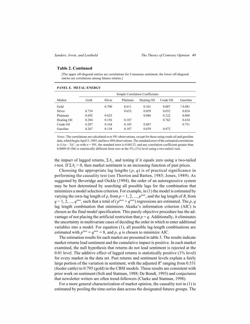
Sanders, Irwin, and Leuthold The Theory of Contrary Opinion 49
Table 2. Continued[The upper off-diagonal entries are correlations for Consensus sentiment; the lower off-diagonalentries are correlations among futures returns.]
PANEL E. METAL/ENERGY
Simple Correlation Coefficients
Market Gold Silver Platinum Heating Oil Crude Oil Gasoline
Gold 0.700 0.611 0.101 0.087 !0.081 Silver 0.734 0.653 0.059 0.032 0.024Platinum 0.692 0.625 0.086 0.122 0.068Heating Oil 0.284 0.156 0.187 0.762 0.634Crude Oil 0.287 0.164 0.185 0.887 0.751Gasoline 0.267 0.134 0.187 0.839 0.872
Notes: The correlations are calculated over 591 observations, except for those using crude oil and gasolinedata, which begin April 5, 1985, and have 494 observations. The standard error of the estimated correlationsis (1/(n – 3))½, so with n = 591, the standard error is 0.04123, and any correlation coefficient greater than0.0809 (0.106) is statistically different from zero at the 5% (1%) level using a two-tailed t-test.
the impact of lagged returns, Σ bj, and testing if it equals zero using a two-tailedt-test. If Σ bj > 0, then market sentiment is an increasing function of past prices.
Choosing the appropriate lag lengths ( p, q) is of practical significance inperforming the causality test (see Thorton and Batten, 1985; Jones, 1989). Assuggested by Beveridge and Oickle (1994), the order of an autoregressive systemmay be best determined by searching all possible lags for the combination thatminimizes a model selection criterion. For example, in (1) the model is estimated byvarying the own-lag length of ρt from p = 1, 2, ..., pmax, and the lag length of Rt fromq = 1, 2, ..., qmax, such that a total of ( pmax × qmax) regressions are estimated. The p, qlag length combination that minimizes Akaike’s information criterion (AIC) ischosen as the final model specification. This purely objective procedure has the ad-vantage of not placing the artificial restriction that p = q. Additionally, it eliminatesthe uncertainty in multivariate cases of deciding the order in which to enter additionalvariables into a model. For equation (1), all possible lag-length combinations areestimated with pmax = qmax = 8, and p, q is chosen to minimize AIC.
The estimation results for each market are presented in table 3. The results indicatemarket returns lead sentiment and the cumulative impact is positive. In each marketexamined, the null hypothesis that returns do not lead sentiment is rejected at the0.01 level. The additive effect of lagged returns is statistically positive (1% level)for every market in the data set. Past returns and sentiment levels explain a fairlylarge portion of the variation in sentiment, with the adjusted R2 ranging from 0.531(feeder cattle) to 0.795 (gold) in the CBSI models. These results are consistent withprior work on sentiment (Solt and Statman, 1988; De Bondt, 1993) and conjecturesthat newsletter writers are often trend-followers (Clarke and Statman, 1998).
For a more general characterization of market opinion, the causality test in (1) isestimated by pooling the time-series data across the designated futures groups. The

50 Spring 2003 Journal of Agribusiness
Table 3. Granger Causality Test for Individual Futures Markets, ReturnsLead Sentiment (May 1983SSSSSeptember 1994)
Equation (1) causality test: ρt ' c0 % jp
i'1aiρt&i %j
q
j'1bj Rt&j % et
Market p, q p-Value Σ bj t-Statistic p-Value Adjust. R2χ2[q]
Grain: Corn 1, 2 39.56 0.000 152.6 4.94 0.000 0.761 Wheat 1, 1 63.83 0.000 140.7 7.98 0.000 0.741 Soybeans 2, 2 23.70 0.000 135.3 4.17 0.000 0.701 Soybean Meal 1, 2 42.64 0.000 172.9 5.45 0.000 0.658 Soybean Oil 2, 2 45.70 0.000 178.5 6.29 0.000 0.653Livestock: Live Cattle 1, 6 73.92 0.000 424.3 5.67 0.000 0.608 Feeder Cattle 4, 1 43.17 0.000 266.1 6.57 0.000 0.531 Live Hogs 2, 2 89.65 0.000 183.8 3.96 0.000 0.675 Pork Bellies 2, 3 54.17 0.000 79.3 3.96 0.000 0.630Food/Fiber: Coffee 3, 3 92.76 0.000 211.7 7.65 0.000 0.652 Sugar 3, 2 60.91 0.000 90.2 6.75 0.000 0.782 Cocoa 2, 2 81.92 0.000 175.2 7.64 0.000 0.631 Orange Juice 5, 2 37.82 0.000 175.6 5.71 0.000 0.693 Cotton 5, 2 68.17 0.000 215.8 6.75 0.000 0.715 Lumber 1, 2 63.92 0.000 155.6 6.52 0.000 0.608Financial: Deutsche Mark 2, 2 97.44 0.000 379.8 7.23 0.000 0.759 Swiss Franc 2, 3 100.50 0.000 460.7 7.42 0.000 0.769 Japanese Yen 1, 5 73.15 0.000 685.8 6.47 0.000 0.745 British Pound 4, 3 81.07 0.000 466.3 6.52 0.000 0.759 Canadian Dollar 3, 2 59.12 0.000 917.5 6.84 0.000 0.688 Treasury Bills 4, 1 66.43 0.000 219.4 8.15 0.000 0.679 Treasury Bonds 4, 2 106.30 0.000 388.3 8.22 0.000 0.727Metal/Energy: Gold 2, 2 71.74 0.000 282.5 7.59 0.000 0.795 Silver 4, 6 98.77 0.000 201.8 4.71 0.000 0.709 Platinum 2, 2 73.41 0.000 213.4 7.91 0.000 0.703 Heating Oil 1, 1 51.06 0.000 89.4 7.14 0.000 0.645 Crude Oil 4, 1 40.55 0.000 65.5 6.36 0.000 0.683 Gasoline 4, 2 30.15 0.000 119.2 5.03 0.000 0.587
Notes: The model is estimated with OLS, and the Wald χ2 statistic tests the null, H0: bj = 0, œ j. The cumulativeimpact of returns is calculated, Σbj, and tested against the null, H0: Σbj = 0, with a two-tailed t-test. All modelsare estimated over 536 weekly observations, except for those involving crude oil and gasoline, which are esti-mated over 438 observations.

Sanders, Irwin, and Leuthold The Theory of Contrary Opinion 51
7 Implicitly, it is assumed sentiment is endogenous and impacted by an exogenous shock to returns.8 The one standard deviation shocks to weekly returns (in parentheses) for each group are as follows: grain (0.029),
livestock (0.029), food/fiber (0.042), financial (0.013), and metal/energy (0.036).9 The impulse response functions decline toward their long-run or total multiplier which is zero, as is the case for
any stationary series.
pooled cross-sectional time-series models are estimated using the generalized leastsquares (GLS) procedure of Kmenta (1986, pp. 616S635) correcting for cross-sectional correlation and heteroskedasticity. The lag lengths for the pooled regres-sions are specified by choosing the maximum p and the maximum q from among theindividual market specifications within each group. For instance, in the grain group,the maximum p is 2 (soybeans and soy oil) and the maximum q is 2 (corn, soybeans,soy meal, and soy oil); therefore, the pooled grain model’s lag structure is 2,2. Whilethis specification procedure may overspecify lag structures at the expense of statis-tical power, it assures the model does not suffer from an underspecification bias.
The estimated pooled models are presented in table 4. For each pooled regression,the null hypothesis that returns do not lead sentiment (i.e., bj = 0, œ j) is tested witha Wald Chi-squared test, and the cumulative impact of lagged returns is again testedwith a two-tailed t-test (i.e., Σbj = 0). Certain important characteristics of sentimentare evident in the results. First, across groups, sentiment follows a fairly strongpositive autoregressive process, with first-order coefficients around 0.65. Second,a statistically significant positive relationship between sentiment and returns isdemonstrated at one- and two-week lags for all the groups. For instance, in grains,a 1% weekly return results in sentiment increasing by 1.26% the following week and0.376% the week after that. For all the groups, the null that returns do not lead senti-ment can be rejected at the 1% level, and the cumulative impact of lagged returnsis significantly positive (1% level).
To illustrate the behavior of sentiment, the impulse response function for a onestandard deviation shock to returns is calculated (see Harvey, 1991, p. 234).7 Thegraphs in figure 2 show the impulse response functions for the pooled sentimentmodels. This figure reveals that a one standard deviation shock in weekly returnscauses the greatest initial increase in food/fiber market sentiment (panel C).8 Notably,the impact on metal/energy (panel E) and financial (panel D) market sentiment doesnot reach a peak until two weeks after the initial shock. All of the response functionsdecline rather smoothly and at similar rates, except for the livestock group (panel B)where extrapolative effects are less pronounced.9 In total, the pooled models stronglysuggest the sentiment levels are caused by returns, and newsletter writers in aggregatemay be trend-followers. These results are consistent with those documented by Soltand Statman (1988) and De Bondt (1993) for retail stock market speculators.
Based on the presented results, two points are clear. First, any test of market senti-ment’s usefulness as a contrary market indicator must be careful to include only pastvalues of sentiment to avoid the contemporaneous correlations documented in table1. Second, given the strong evidence that returns lead sentiment, a regression-basedpredictive model which does not include past returns is potentially misspecified.Therefore, Granger’s causality test that sentiment leads returns is a natural extension

52 Spring 2003 Journal of Agribusiness
Table 4. Granger Causality Test for Pooled Futures Market Groups, ReturnsLead Sentiment (May 1983SSSSSeptember 1994)
Independent Market Group
Variable Grain Livestock Food/Fiber Financial Metal/Energy
Intercept 11.09(16.9)
12.03(12.3)
10.45(17.0)
10.33(16.6)
10.02(13.7)
ρt!1 0.664(31.2)
0.617(26.1)
0.645(33.2)
0.692(39.2)
0.685(32.7)
ρt!2 0.091(4.57)
0.049(1.78)
0.028(1.21)
0.021(0.96)
0.026(1.02)
ρt!3 — 0.022(0.80)
0.044(1.94)
!0.003 (!0.15)
0.029(1.15)
ρt!4 — 0.053(2.32)
0.011(0.49)
0.052(3.11)
0.022(1.07)
ρt!5 — — 0.026(1.54)
— —
Rt!1 126.5(14.6)
95.9(11.6)
104.0(18.8)
233.8(17.5)
94.1(13.8)
Rt!2 37.6(4.44)
25.9(3.03)
32.9(5.64)
79.6(5.67)
29.5(4.15)
Rt!3 — 4.09(0.47)
5.22(0.90)
28.4(2.01)
4.64(0.65)
Rt!4 — !5.76 (!0.78)
28.50(2.11)
!1.95 (!0.28)
—
Rt!5 — !7.65 (!0.94)
!5.93 (!0.44)
9.54(1.38)
—
Rt!6 — !4.67 (!0.58)
— !3.37 (!0.50)
—
Σbj 164.1(12.80)
107.8(4.86)
142.2(13.20)
364.6(10.70)
132.4(7.24)
aχ2
[q] 221.6 143.9 368.7 364.6 202.7
Buse’s R2 0.667 0.545 0.683 0.671 0.653
Note: The t-statistics (in parentheses) test if the coefficient equals zero, with degrees of freedom equal toN(K – ( p + q + 1), where N = 536 (438 for metal/energy) and K = number of markets in the group.a All the statistics reject that the coefficients on lagged returns are zero at the 1% level.χ2
[q]
of the work presented thus far, and it is an appropriately specified time-series test forsentiment’s value as a contrary indicator.
Tests for Return Predictability
Two different time-series tests of return predictability are employed. The first isa general test based on a Granger causality specification parallel to that presented inequation (1). The second is a more specialized test of contrary opinion based on themarket-timing framework developed by Cumby and Modest (1987).

Sanders, Irwin, and Leuthold The Theory of Contrary Opinion 53
Figure 2. Impulse response functions for futures market groups,return impact on market sentiment (May 1983SSSSSeptember 1994)

54 Spring 2003 Journal of Agribusiness
Causality Tests
Following the specification and estimation procedures presented for equation (1), thelinear linkages between returns and sentiment are examined using the bivariateGranger test:
(2) Rt ' k0 % jm
i'1αi Rt&i %j
n
j'1βjρt&j % gt ,
where Rt and ρt are futures returns and noise trader sentiment, respectively, and gt isa white noise error term. Sentiment leads returns in equation (2) if market sentimentis useful in predicting returns, and it is tested under the null of βj = 0, œ j. Further-more, the cumulative impact of market sentiment on returns is tested under the nullof Σβj = 0. Rational expectations is also tested under the full orthogonality condition:βj = αi = 0, œ i, j. Again, to increase the power of these tests, they are estimated overpooled cross-sectional time-series data using the futures groups presented in table 1.
Equation (2) provides a well-specified and general means of testing the orthogon-ality condition implied by market rationality. If, however, sentiment is a useful con-trary indicator for market returns, then there will be a negative relationship betweensentiment and returns—i.e., high (low) sentiment predicts negative (positive) returns.A contrarian relationship should be captured in (2) by finding that sentiment leadsreturns βj … 0, œ j, and the cumulative impact of sentiment on returns is negative(Σβj < 0). The opposite is true for a positive impact (βj … 0, œ j, and Σβj > 0).
The causality test results for individual markets are presented in table 5. The firstχ2 statistic (column 3) tests the null that sentiment does not lead returns, and thet-statistic (column 5) tests if the sum of lagged sentiment coefficients equals zero.The second χ2 statistic (column 6) tests the full orthogonality condition. The firstresult of importance is that lagged sentiment did not even enter 14 of the 28 regres-sion models. For the remaining models, the null hypothesis that sentiment does notlead returns is rejected for two markets (lumber and Treasury bills) at the 5% level,and four more markets (feeder cattle, cocoa, orange juice, and live hogs) at the 10%level. The total of six rejections is more than would be expected by chance alone(0.10 × 28 = 2.8 rejections).
While there is some evidence of a relationship between sentiment and subsequentfutures returns, the direction of the relationship is not consistent. Trade sources(e.g., CONSENSUS) tout sentiment as a contrary indicator, but the t-statistics for H0:Σβj = 0 reveal that the sum of lagged sentiment coefficients is not consistentlynegative. The sum is significantly negative in only two cases (live hogs and cocoa).Further, nine of the 14 t-statistics are positive, indicating a tendency toward continu-ation instead of reversal.
The second χ2 statistic (column 6) in table 5 tests the null hypothesis that neithersentiment nor past returns lead future returns, i.e., returns are not predictable withthe information contained in past returns and sentiment. This null is rejected in 13markets at the 10% level or higher. Of the 13 rejections, eight are in markets wherethe first χ2 test did not reject the null, and the rejections are concentrated among the

Sanders, Irwin, and Leuthold The Theory of Contrary Opinion 55
Table 5. Granger Causality Test for Individual Futures Markets, SentimentLeads Returns (May 1983SSSSSeptember 1994)
Equation (2) causality test: Rt ' k0 % jm
i'1αiRt&i %j
n
j'1βjρt&j % gt
[1] [2] [3] [4] [5] [6] [7] [8]
Market m, n p-Value t-Statistic p-Value Adjust. R2χ2[n] χ2
[m%n]
Grain: Corn 5, 0 — — — 5.72 0.334 0.017 Wheat 0, 1 0.17 0.679 !0.41 0.17 0.679 !0.001 Soybeans 3, 1 2.30 0.129 !1.51 4.82 0.306 0.008 Soybean Meal 3, 0 — — — 4.31 0.230 0.009 Soybean Oil 3, 0 — — — 3.45 0.327 0.010Livestock: Live Cattle 6, 0 — — — 11.95 0.063 0.015 Feeder Cattle 2, 3 7.48 0.058 0.76 10.61 0.059 0.017 Live Hogs 1, 3 6.39 0.094 !2.05 17.13 0.002 0.024 Pork Bellies 1, 0 — — — 0.72 0.393 !0.001Food/Fiber: Coffee 1, 0 — — — 0.22 0.638 !0.002 Sugar 0, 1 2.11 0.146 1.45 2.11 0.146 0.002 Cocoa 0, 1 3.21 0.073 !1.79 3.21 0.073 0.004 Orange Juice 1, 5 10.32 0.066 2.62 31.69 0.000 0.041 Cotton 4, 0 — — — 12.69 0.012 0.028 Lumber 2, 2 18.68 0.000 !0.49 25.24 0.000 0.059Financial: Deutsche Mark 0, 1 1.21 0.271 1.09 1.21 0.271 0.000 Swiss Franc 3, 0 — — — 6.19 0.102 0.009 Japanese Yen 0, 1 2.16 0.141 1.47 2.16 0.141 0.002 British Pound 3, 0 — — — 6.86 0.076 0.009 Canadian Dollar 0, 1 0.53 0.462 0.73 0.53 0.462 !0.001 Treasury Bills 0, 5 16.86 0.005 0.06 16.86 0.005 0.015 Treasury Bonds 1, 0 — — — 0.64 0.422 !0.001Metal/Energy: Gold 0, 1 0.31 0.574 0.56 0.31 0.574 !0.001 Silver 6, 0 — — — 9.32 0.156 0.016 Platinum 6, 1 2.55 0.111 1.59 13.72 0.056 0.015 Heating Oil 3, 0 — — — 8.96 0.029 0.022 Crude Oil 3, 0 — — — 6.79 0.078 0.013 Gasoline 3, 0 — — — 8.77 0.032 0.025
Notes: The model is estimated with OLS, and the first Wald χ2 statistic (column 3) tests the null, H0: βj = 0,œ j. The t-statistic tests that the sum of the lagged sentiment coefficients equals zero, Σβj = 0. The second χ2
statistic (column 6) tests full orthogonality, H0: αi = 0 and βj = 0, œ i, j. The model is estimated over 536weekly observations, except for those regressions involving crude oil and gasoline, which have 438 obser-vations.

56 Spring 2003 Journal of Agribusiness
10 The individual models were also estimated in a seemingly unrelated regression (SUR) framework, but the resultswere not materially different from the OLS estimations.
Table 6. Granger Causality Test for Pooled Futures Market Groups, Senti-ment Leads Returns (May 1983SSSSSeptember 1994)
Independent Market Group, Coefficient × 10!2
Variable Grain Livestock Food/Fiber Financial Metal/Energy
Intercept 0.0149(0.10)
!0.0699 (!0.40)
!0.1658 (!0.83)
0.0178(0.95)
!0.1596 (!0.99)
Rt!1 0.4028(0.20)
2.4092(1.05)
6.5781(3.34)
!2.7300 (!1.63)
!3.7200 (!1.84)
Rt!2 5.6255(2.77)
!2.438 (!1.05)
4.3187(2.07)
3.8714(2.29)
3.6352(1.75)
Rt!3 7.2097(3.59)
2.5207(1.10)
2.4519(1.17)
2.8223(1.67)
4.6910(2.28)
Rt!4 0.4432(0.23)
!0.1779 (!0.07)
4.9758(2.39)
— 1.5412(0.75)
Rt!5 !2.1835 (!1.11)
!4.975 (!2.22)
— — !4.5359 (!2.25)
Rt!6 — 2.7824(1.23)
— — !1.8822 (!0.89)
ρt!1 !0.0005 (!0.10)
0.0012(0.32)
!0.0135 (!2.24)
0.0001(0.25)
0.0028(0.89)
ρt!2 — 0.0040(0.94)
0.0155(2.16)
!0.0004 (!0.54)
—
ρt!3 — !0.0003 (!0.09)
!0.0099 (!1.38)
!0.0004 (!0.65)
—
ρt!4 — — !0.0010 (!0.14)
0.0013(2.13)
—
ρt!5 — — 0.0127(2.32)
!0.0009 (!1.79)
—
0.051χ2[n]
[0.821]2.76
[0.431]15.08
[0.010]5.40
[0.368]0.80
[0.370]
22.28χ2[m%n]
[0.001]13.75
[0.131]35.69
[0.000]15.26
[0.054]19.98
[0.005]
Buse’s R2 0.006 0.001 0.009 0.002 0.006
Notes: The t-statistics (in parentheses) test if the coefficient equals zero, with degrees of freedom equal toN(K – (m + n + 1), where N = 536 (438 for metal/energy) and K = number of markets in the group. The first(second) χ2 statistic tests H0: βj = 0 (and αi = 0), œ i, j [with p-values in brackets].
food/fiber and metal/energy groups. Although not presented, in the markets wherethe full orthogonality null is rejected, the rejection primarily stems from low-orderpositive autocorrelation in returns.
The pooled causality results are presented in table 6. Pooled models were estimatedwith Kmenta’s cross-sectionally correlated and heteroskedastic GLS procedure.10

Sanders, Irwin, and Leuthold The Theory of Contrary Opinion 57
11 The sum of lagged sentiment coefficients is not significantly different from zero for the food/fiber group.
Figure 3. Impulse response function for the food/fiber market group,market sentiment impact on return (May 1983SSSSSeptember 1994)
The first χ2 statistic (with p-values in brackets) tests the null that sentiment does notlead returns, and the second χ2 statistic tests the full orthogonality condition. Thenull hypothesis that sentiment does not lead returns is rejected for the food/fibergroup only. The full orthogonality null hypothesis is rejected at conventional levelsfor all groups except livestock. Returns in general, and the food/fiber and graingroups in particular, are characterized by positive autocorrelation at short lags withautoregressive parameters along the order of 0.05 to 0.07 in magnitude.
As with the individual market models, the direction of sentiment’s impact onreturns is somewhat inconsistent. For example, the food/fiber group’s sentimentcoefficients are significantly negative at lag one and significantly positive at lagstwo and five.11 The full impulse response to a one standard deviation shock to weeklysentiment is plotted in figure 3 for the food/fiber group. The figure shows there isnot a well-defined response structure for sentiment leading returns. That is, theresponse function takes both positive and negative values before converging to zeroafter seven weeks.
Collectively, the causality models provide some mild evidence that newslettersentiment is useful in predicting market returns. However, the null hypothesis isrejected in a relatively small number of the markets. Furthermore, the direction ofsentiment’s impact is not consistent across markets. The small amount of evidencewhich does exist would suggest price continuation over weekly intervals, not pricereversals. This evidence is not supportive of using sentiment as a contrary indicator.

58 Spring 2003 Journal of Agribusiness
12 The OLS error terms are tested for heteroskedasticity using White’s test, and for autocorrelation using theLagrange multiplier test. If the errors are heteroskedastic, then the model is estimated using White’s heteroskedasticconsistent covariance estimator, and if the errors are autocorrelated, then the Newey-West covariance estimator isutilized (Hamilton, 1994, p. 281).
However, the findings are consistent with those reported by Wang (2001) for CFTCsmall speculators in agricultural futures markets.
Cumby-Modest Test
While the causality test results presented above do not indicate a consistent relation-ship between noise trader sentiment and subsequent futures price movements, it maybe possible that a relationship exists, but only at extreme levels of sentiment(CONSENSUS; Wang, 2001). The market-timing framework proposed by Cumbyand Modest (1987) can be used to determine whether extreme sentiment readingsprovide market signals. Given a definition of extremely high and low sentiment levels(KH and KL, respectively), the Cumby-Modest (C-M) test is based on the followingOLS regression:
(3) Rt ' α % β1HIt&1 % β2 LOt&1 % gt ,
where HIt!1 = 1 if ρt!1 > KH, and HIt!1 = 0 otherwise; LOt!1 = 1 if ρt!1 < KL, andLOt!1 = 0 otherwise. If the mean return conditioned on extreme optimism (α + β1) orpessimism (α + β2) is different from the unconditional mean (α), then timing abilityis demonstrated. The null hypothesis of no predictability, H0: β1 = β2 = 0, is testedagainst the alternative of significant timing ability, HA: β1 … 0 or β2 … 0. “Contraryopinion” would suggest that β1 < 0 or β2 > 0, indicating extreme sentiment is nega-tively related to returns.
Consensus, Inc. suggests that sentiment outside the range of (25, 75) denotes amarket approaching extreme conditions. For the initial C-M tests, extreme sentimentis defined by these levels plus a factor of five to assure that the extremes composea small percentage of the total observations. The C-M test results for individualmarkets with KH = 80 and KL = 20 are presented in table 7.12 For individual markets,the number of extreme observations constitutes from 4.3% (23) to 30% (161) of the536 total observations for each market. Based on χ2 statistics, the null hypothesis ofno timing ability (β1 = β2 = 0) is rejected for three markets (live cattle, Canadiandollar, gasoline) at the 5% level and two more markets (soybeans, cocoa) at the10% level. Again, the five rejections are more than would be expected by chance(0.10 × 28 = 2.8 rejections). There also are four cases where an individual coefficientis significantly different from zero (β2 for wheat, Japanese yen, platinum, and crudeoil), but the joint test is insignificant. Finally, it is worth noting that only one of therejections (cocoa) is common to both the C-M and causality tests.
While there is evidence of a significant relationship between extreme sentimentand returns, the direction of the relationship is, if anything, one of continuation.

Sanders, Irwin, and Leuthold The Theory of Contrary Opinion 59
Table 7. Cumby-Modest Test for Individual Futures Markets (May 1983SSSSSeptember 1994)
Equation (3) Cumby-Modest regression: Rt ' α % β1HIt&1 % β2LOt&1 % gt
MarketExtreme
Observations α × 10!2 β1 × 10!2 β2 × 10!2 p-Valueχ2[2]
Grain: Corn 76 !0.1472
(!1.09)0.7522(1.03)
!0.0672 (!0.18)
1.09 0.579
Wheat 92 !0.0869 (!0.71)
0.4283(0.82)
0.6477(1.89)
4.05 0.131
Soybeans 47 !0.1400 (!1.03)
0.5031(0.49)
0.7299(2.27)
5.36 0.068
Soybean Meal 106 0.0198(0.12)
!0.3885 (!0.55)
!0.1124 (!0.38)
0.42 0.801
Soybean Oil 126 0.0538(0.29)
0.5080(0.50)
!0.5283 (!1.60)
2.99 0.223
Livestock: Live Cattle 23 0.1659
(1.88)!0.0224 (!0.06)
2.0730(3.13)
9.83 0.007
Feeder Cattle 78 0.0831(1.02)
0.1825(0.71)
0.2078(0.56)
0.72 0.696
Live Hogs 23 0.2596(2.02)
!0.9115 (!0.61)
!0.0704 (!0.10)
0.39 0.822
Pork Bellies 88 !0.3557 (!1.49)
1.3560(0.84)
0.1414(0.22)
0.74 0.689
Food/Fiber: Coffee 113 !0.2414
(!1.24)0.3544(0.23)
0.1850(0.40)
0.21 0.901
Sugar 117 !0.4081 (!1.36)
0.8003(0.87)
!0.9866 (!1.21)
2.54 0.279
Cocoa 110 !0.4495 (!2.36)
0.9907(0.91)
0.9082(2.05)
4.82 0.089
Orange Juice 161 0.2338(1.18)
0.5623(0.83)
!0.5112 (!1.63)
3.73 0.154
Cotton 101 0.1648(1.13)
0.5484(0.99)
!0.4501 (!1.46)
3.54 0.170
Lumber 120 0.0235(0.12)
!1.2387 (!1.08)
!0.0762 (!0.18)
1.18 0.553
Financial: Deutsche Mark 105 0.0626
(0.74)0.7518(0.21)
!0.7747 (!0.40)
0.23 0.890
Swiss Franc 115 0.0103(0.11)
0.2532(0.73)
0.0434(0.21)
0.56 0.756
Japanese Yen 98 0.1735(2.38)
!0.2310 (!0.70)
!0.3250 (!1.71)
3.22 0.198
( continued . . . )

60 Spring 2003 Journal of Agribusiness
13 In the text, the C-M coefficients are always referred to as the change in returns or expected percentage pricechange, relative to the unconditional return. This is in contrast to the total expected return. For instance, when theCBSI is below 20, the expected weekly live cattle return increases by 2.07%, but the total expected return is 2.24%(2.07 + 0.17).
Table 7. Continued
MarketExtreme
Observations α × 10!2 β1 × 10!2 β2 × 10!2 p-Valueχ2[2]
Financial (cont’d): British Pound 130 0.0355
(0.39)0.3856(1.46)
!0.0264 (!0.11)
2.23 0.328
Canadian Dollar 98 0.0582(2.13)
!0.1064 (!0.72)
!0.1877 (!2.46)
6.29 0.043
Treasury Bills 98 0.0019(2.21)
0.0305(1.34)
!0.0190 (!0.48)
2.17 0.337
Treasury Bonds 39 0.0173(2.44)
!0.5901 (!0.11)
!0.4312 (!1.44)
2.09 0.351
Metal/Energy: Gold 101 !0.0180
(!2.00)0.4368(0.84)
0.0685(0.24)
0.75 0.687
Silver 68 !0.4169 (!2.81)
0.7366(0.80)
0.5552(0.96)
1.58 0.452
Platinum 114 !0.4510 (!0.32)
0.3082(0.29)
!0.5878 (!1.76)
3.26 0.196
Heating Oil 130 0.0923(0.43)
!1.1126 (!1.08)
!0.6281 (!0.12)
1.18 0.553
Crude Oil 67 0.3340(1.38)
!0.8007 (!0.94)
!1.7014 (!1.67)
3.36 0.186
Gasoline 120 0.4406(1.82)
!0.1653 (!2.44)
!0.8561 (!1.33)
6.87 0.032
Notes: The model is estimated with OLS, where HIt!1 = 1 if ρt!1 > KH , and HIt!1 = 0 otherwise; LOt!1 = 1 if ρt!1 < KL,and LOt!1 = 0 otherwise; and KH = 80, KL = 20. Values in parentheses are t-statistics, and the Chi-squared test is ajoint test of the null, H0: β1 = β2 = 0. All models are estimated over 536 weekly observations, except for thoseinvolving crude oil and gasoline, which are estimated over 438 observations.
Returns increase (decrease) after high (low) sentiment, rather than reverse. In addi-tion, there is variation in the coefficient signs for those markets where the null isrejected. For instance, if the CBSI is below 20, then the following week nearby livecattle returns increase by 2.07% on average, while Canadian dollar returns fall0.188%.13
Pooled C-M test results with KH = 80 and KL = 20 are presented in panel B oftable 8. The pooled C-M models are estimated using Kmenta’s cross-sectionallycorrelated, heteroskedastic, and timewise autoregressive GLS estimation technique.Of the five market groups, the null of no market timing is rejected at the 5% levelfor the grains and at the 10% level for the financials. For example, the estimatedcoefficients show weekly grain futures returns increase by 0.4029% after sentiment

Sanders, Irwin, and Leuthold The Theory of Contrary Opinion 61
Table 8. Cumby-Modest Test for Pooled Futures Market Groups (May 1983SSSSSeptember 1994)
Equation (3) Cumby-Modest regression: Rt ' α % β1HIt&1 % β2LOt&1 % gt
PANEL A. KH = 75, KL = 25
Group α × 10!2 β1 × 10!2 β2 × 10!2 p-Valueχ2[2]
Grain !0.0416 (!0.43)
0.3687(2.83)
0.0273(0.36)
8.16 0.016
Livestock 0.1239(1.57)
0.2009(1.53)
0.1462(1.20)
3.69 0.157
Food/Fiber !0.0245 (!0.28)
!0.0703 (!0.28)
0.0239(0.15)
0.16 0.943
Financial 0.0096(1.16)
0.0087(0.37)
0.0089(0.51)
0.36 0.834
Metal/Energy !0.0263 (!0.29)
0.1259(0.74)
!0.1833 (!1.75)
3.78 0.151
PANEL B. KH = 80, KL = 20
Group α × 10!2 β1 × 10!2 β2 × 10!2 p-Valueχ2[2]
Grain !0.0308 (!0.32)
0.4029(2.43)
0.0689(0.73)
6.44 0.039
Livestock 0.1519(1.95)
!0.0070 (!0.04)
!0.0338 (!0.20)
0.04 0.978
Food/Fiber !0.0463 (!0.58)
0.4979(1.54)
0.0116(0.06)
2.36 0.307
Financial 0.0117(1.52)
0.0549(1.82)
!0.0209 (!1.02)
4.65 0.098
Metal/Energy !0.0362 (!0.41)
0.2118(0.86)
!0.2311 (!1.80)
4.07 0.131
PANEL C. KH = 85, KL = 15
Group α × 10!2 β1 × 10!2 β2 × 10!2 p-Valueχ2[2]
Grain !0.0113 (!0.12)
0.4166(1.58)
0.0027(0.02)
2.49 0.286
Livestock 0.1563(2.02)
!0.0598 (!0.22)
!0.2856 (!1.29)
1.72 0.423
Food/Fiber !0.0362 (!0.46)
!0.0515 (!0.11)
0.1294(0.58)
0.36 0.833
Financial 0.0122(1.60)
0.0561(1.19)
!0.0156 (!0.65)
1.91 0.385
Metal/Energy !0.0393 (!0.45)
0.1591(0.47)
!0.2148 (!1.32)
1.98 0.372
Notes: The model is estimated over N cross-sections and T time-series observations, where HIt!1 = 1 if ρt!1 > KH,and HIt!1 = 0 otherwise; LOt!1 = 1 if ρt!1 < KL , and LOt!1 = 0 otherwise. The t-statistics (in parentheses) test thatparameter values are zero, and the χ2 tests the joint null, H0: β1 = β2 = 0. All models are estimated over 536 weeklyobservations, except the metal/energy group, which is estimated over 438 observations. Each pooled regressionhas N × T cross-sectional time-series observations, where T = 536 (or 438) and N is the number of marketscomprising the group.

62 Spring 2003 Journal of Agribusiness
14 While these returns are statistically significant, their economic significance is debatable. It is not the intent ofthis study to search for an economically significant trading strategy. Instead, we are simply investigating the time-series predictability of returns.
readings above 80%, and increase by 0.0689% after sentiment readings below20%.14
Parameter sensitivity is explored by altering the definition of extreme sentiment.In panel A of table 8, KH = 75 and KL = 25, while in panel C, KH = 85 and KL = 15.At decreased extremes (panel A), the grain model still displays statistically signifi-cant timing ability, but when the extreme sentiment definitions are widened (panelC), none of the pooled models reject the null hypothesis. These results suggest thatthe impact of market sentiment is quite sensitive to alternative definitions of extremeindex values.
Overall, the C-M test results indicate some evidence of a predictive relationshipbetween extreme sentiment and subsequent futures returns. The evidence is strongestfor grain futures markets. However, the relationship is indicated for only a limitednumber of the markets, it is sensitive to the definition of “extreme” sentiment, andthe direction of extreme sentiment’s impact generally is that of continuation. Theseresults do not support the use of the sentiment index as a contrary market indicator,even at extreme levels. The tenuous causal relationships between sentiment andreturns are consistent with Fisher and Statman’s (2000) results for newsletter writersin equity markets and Wang’s (2001) findings for CFTC small speculators in agri-cultural futures.
Summary and Conclusions
The theory of contrary opinion predicts price reversals following extremes in marketsentiment. This analysis tests return predictability in futures markets using a direct,or survey-based, measure of sentiment. Findings show the Consensus Index ofBullish Market Opinion primarily reflects the opinions of newsletter writers and thecorresponding market positions of their primary audience—retail futures speculators.The lead-lag relationships between sentiment and futures market returns are investi-gated within a Granger causality framework. The results suggest that sentiment isan increasing function of past futures returns over at least the previous two weeks,and retail futures speculators may be trend-followers who act in unison to correlatedmarket signals (past returns). This characterization is consistent with the theoretical“noise traders” of De Long et al. (1990a,b), and the results can have ramificationsfor interpreting and testing noise trader models (Sanders, Irwin, and Leuthold, 2000).
In this research, market sentiment is found to have little predictive power in futuresmarkets. Time-series regressions (Granger causality tests) are specified to test if thelevel of noise trader sentiment consistently predicts subsequent futures price move-ments. The predictive ability of extremely high or low sentiment is also tested in aCumby-Modest (1987) market-timing framework. The time-series regressions providesome evidence that noise trader sentiment is useful in predicting market returns,

Sanders, Irwin, and Leuthold The Theory of Contrary Opinion 63
particularly when sentiment is at extreme levels. However, relationships are presentfor only a limited number of the markets, and the direction of sentiment’s impactgenerally is inconsistent. The relationship, if any, tends toward continuation.Specifically, there is little or no evidence supporting market reversals or “contraryopinion.” This conclusion is fairly consistent across the 28 futures markets examined.Therefore, practitioners who rely solely on this type of indicator may be misguided.The results may also provide interpretive evidence for different theoretical modelswhich suggest sentiment can influence market returns (e.g., Cutler, Poterba, andSummers, 1989; Barberis, Shleifer, and Vishny, 1998).
This research focuses on one sentiment index, the Consensus Index of BullishMarket Opinion, which reflects the sentiment of market newsletters. As pointed outby Fisher and Statman (2000), the results could vary using the sentiment of anothersegment of market participants (see also Wang, 2001). Likewise, sentiment couldimpact other aspects of price behavior, such as volatility. We concur with Fisher andStatman that this line of research needs to be broadened to additional markets, alter-native forms of price behavior, and other measures of sentiment.
References
Barberis, N., A. Shleifer, and R. Vishny. (1998). “A model of investor sentiment.”Journal of Financial Economics 49, 307S343.
Beveridge, S., and C. Oickle. (1994). “A comparison of Box-Jenkins and objective meth-ods for determining the order of a non-seasonal ARMA Model.” Journal of Fore-casting 13, 419S434.
Brennan, M. J. (1995). “The individual investor.” Journal of Financial Research 18,59S74.
Brown, G. W. (1999). “Volatility, sentiment, and noise traders.” Financial AnalystsJournal 55, 82S90.
Brown, G. W., and M. T. Cliff. (2001, September). “Investor sentiment and the near-term stock market.” Financial Economics Network, Capital Markets Abstracts: MarketEfficiency. Working paper, Kenan-Flagler Business School, University of NorthCarolina-Chapel Hill.
Canoles, B. W., S. Thompson, S. Irwin, and V. G. France. (1998). “An analysis of theprofiles and motivations of habitual commodity speculators.” Journal of Futures Mar-kets 18, 765S801.
Clarke, R. G., and M. Statman. (1998). “Bullish or bearish.” Financial Analysts Journal54, 63S72.
Consensus, Inc. (1995, February 17). CONSENSUS: National Futures and FinancialWeekly [Kansas City, MO], Vol. XXV, No. 7.
Consensus, Inc. (2001, November 15). Sentiment index. Online website. Available athttp://www.consensus-inc.com/.
Cumby, R. E., and D. M. Modest. (1987). “Testing for market timing ability: A frame-work for forecast evaluation.” Journal of Financial Economics 19, 169S189.
Cutler, D. M., J. M. Poterba, and L. H. Summers. (1989). “Speculative dynamics and therole of feedback traders.” American Economic Review 80, 63S68.

64 Spring 2003 Journal of Agribusiness
Daily % Bullish. (2000, October). Online website. Available at http://www.homestead.com/dailybullish/.
De Bondt, W. F. M. (1993). “Betting on trends: Intuitive forecasts of financial risk andreturn.” International Journal of Forecasting 9, 355S371.
De Long, J. B., A. Shleifer, L. H. Summers, and R. J. Waldmann. (1990a). “Noise traderrisk in financial markets.” Journal of Political Economy 98, 703S738.
———. (1990b). “Positive feedback investment strategies and destabilizing rationalspeculation.” Journal of Finance 45, 379S395.
Draper, D. W. (1985). “The small public trader in futures markets.” In A. E. Peck (ed.),Futures Markets: Regulatory Issues (pp. 211S269). Washington, DC: American Enter-prise Institute for Public Policy Research.
Elton, E. J., M. J. Gruber, and J. A. Busse. (1998). “Do investors care about sentiment?”Journal of Business 71, 477S501.
Fisher, K. L., and M. Statman. (2000). “Investor sentiment and stock returns.” FinancialAnalysts Journal 56, 16S23.
Greene, W. H. (1993). Econometric Analysis. New York: MacMillan Publishing Co.Hamilton, J. D. (1994). Time Series Analysis. Princeton, NJ: Princeton University Press.Harvey, A. C. (1991). The Econometric Analysis of Time Series, 2nd edition. Cambridge,
MA: MIT Press.Jones, J. (1989). “A comparison of lag-length selection techniques in tests of Granger
causality between money growth and inflation: Evidence for the U.S., 1959S86.”Applied Economics 24, 809S822.
Kmenta, J. (1986). Elements of Econometrics, 2nd edition. New York: Macmillan Pub-lishing Co.
Nagy, R. A., and R. W. Obenberger. (1994, July/August). “Factors influencing individ-ual investor behavior.” Financial Analysts Journal 50, 63S68.
Neal, R., and S. M. Wheatley. (1998). “Do measures of investor sentiment predictreturns?” Journal of Financial and Quantitative Analysis 33, 523S547.
Neill, H. (1960). The Art of Contrary Thinking. Caldwell, OH: Caxton Printers.Sanders, D. R., S. H. Irwin, and R. M. Leuthold. (2000). “Noise trader sentiment in
futures markets.” In B. A. Goss (ed.), Models of Futures Markets (pp. 86S116). NewYork: Routledge.
Simon, D. P., and R. A. Wiggins. (2001). “S&P futures returns and contrary sentimentindicators.” Journal of Futures Markets 21, 447S462.
Smidt, S. (1965). “Amateur speculators.” Cornell Studies in Policy Administration,Cornell University, Ithaca, NY.
Solt, M. E., and M. Statman. (1988, September). “How useful is the sentiment index?”Financial Analysts Journal 44, 45S55.
Teweles, R. J., and F. J. Jones. (1999). The Futures Game: Who Wins, Who Loses, andWhy. New York: McGraw-Hill.
Thorton, D., and D. Batten. (1985). “Lag-length selection and tests of Granger causalitybetween money and income.” Journal of Banking and Finance 17, 164S178.
Wang, C. (2001). “Investor sentiment and return predictability in agricultural futuresmarkets.” Journal of Futures Markets 21, 929S952.