AD-A285 886

S LABORATORY

The Tensor EquationAX + XA = 4D (A, H)With Applications to

Kinematics of Continua

Michael J. Scheidler

ARL-TR-582 September 1994

94-33315

AROVW !0 P2UOCEE

'94-10 26 008

NOTICES

DestToy this report when it is no longer needed. DO NOT relum it to the originator.

Additional copies of this report may be obtained from the National Technical InWormationService, U.S. Department of Commerce, 5285 Port Royal Road. Springfield, VA 22161.

The findings of this report are not to be construed as an official Department of the Armyposition, unless so designated by other authorized documents.

The use of trade names or manufacturers' names in this report does not constituteindorsement of any commercial product.

Form ApprovedREPORT DOCUMENTATION PAGE OMB No 0704 0188

*t)4, tpO .r I buderI I EuII, hIIoI tIpClov(Ifl 'n1 o- a t.uo 'I eMt., a t- o a.I S hu' -V- p -'V,ia -l , ' . th;Ie tO'PC fo, - - - Ip Irp ,,.> I ýI leaP.'1 I "I -It' q J Ata WOO MI

90ther-nq ~ ,Ar.Vrl he dat. le"IdedA and c.-rotettq11 e~ the .,tet', .rf-0n!.) oed lf'"o.,10rj t~'t " t,'~pat ,-h1AL> f,~

1. AGENCY USE ONLY (.eave blank) 12 REPORT DATE • REPOA, TYPE AND DATES COVERED

I Sq~iecther 1994 Final, March 92-March 934. TITLE AND SUBTITLE 5 FUNDING NUMBERS

The Tenaw FquMizo AX + XA = 0 (A, H) With ApplicaiOM to Kinematics ofCo01nun PR: 1L161102AH43

6 AUTHOR(S)

Mbdmei J. $rhk~r

7 PERFORMING ORGANIZAT;ON NAME(S) AND ADORISS(ES) 8 PERFORMING ORGANIZATIONREPORT NUMBER

U.S. Army Re•c aowrATTYN: AMSRL-WTF-TD

Abrdew froving GOmund. MD 21005-5066

9 SPONSORING IONITOqG AGENCY NAME(M: ANr) ADDRESS(US) 10 SPONSORING MONITORINGAGENCY REPORT NUMBER

U.S. A-my Researh LAbormoryATMN: AMSRL.OP-AP-L ARL-TR-582Aberdena Proving Gvmsmd MD 21WO5-50M~

11 SUPPLEMENTA~1V NOTES

12a. DISTRIBUTION AVAILABILITY STATEMENT 12b. DISTRIBUTION CODE

Approved for public rele.me distribution is unlimitr

13. ABSTRACT (Maximum 200 words)

The (second-order) tensor equaton AX + XA = 0 (A, H) is studied for certain isotropic functions 0 (A, H) which arein H. (Qalitauve properties of the solution X and relations between the solutions for various forms of 0 are

lished for an iner pr•uuct sae of arbitrary dimeson. These results, together with Rivlin's identities for tensor

lynomials in two variabs, am applied in three dimensions to obtain new explicit formulas for X in direct tensor notationwell as new derivations of previously known formulas. Several applications to the kinematics o' continua are considered.

14. SUIJECT TERMS Th NUMBER OF PAGLSkineaksti matrix equatom. I _ _ _ _ 42

16. PRICE CODE

17 SECURITY CLASSIFKIATION 1I SECURITY CLASSIFICATION 19. SECURITY CLASWiFIC.-.TION 20 LIIVITATION OF ABSTRACTOF REPORT OF THIS PAGE I OF ABSTRACT

UNITASSIpD• UNCLAMFSIFED UNILASSIFIEI ULNS% ?500, 60' SSOC Standard rormn 298 (Rev 2-89)

P wM bý ANSI Slat LE9-18199'0.1

INTENTIONALLY LEFT BLANK.

Contents

1 Introduction 1

2 The fourth-order tensors LA, MA, and NA 6

3 Some tensor identities in three dimensions 12

4 Existence and uniqueness of solutions.Direct solutions in T(A) 17

5 Direct formulas for LA, MA, and NAin three dimensions 20

6 Applications to kinematics of continua 26

7 Additional kinematic formulas 32

I

•ii

INTMlýONALLY LEFT BLANK.

iv

1 Introduction

A variety of problems in continuum mechanics require the solution X of a linearalgebraic equation of the form

AX + XA = (A, H). (1.1)

Here A, X, and H are second-order tensors (i.e., linear transformations) cn a two- orthree-dimensional inner product space V, and 4(A, H) is an isotropic function of Aand H which is lincar in H.

For example, consider a smooth motion with deformation gradient F.' By thepolar decomposition theorem, F has the unique multiplicative decompositions

F = RU =7 VR, (1.2)

where the proper orthogonal tensor R. is the rotation tensor, and the symmetric,

positive-definite tensors U and V are the right and left stretch tcnsors. Let C and Bdenote the right and left Cauchy-Green tensors:

C = FTF= U 2 and B =FFTI' V 2 . (1.3)

Let the stretching tensor D and the spin tensor W denote the syvmletric and skewparts of the velocity gradient L:

L=D+W, D=svmL= L (L+L T ), W=skwL= I(L--L T ). (1.4)

0

For any tensor field A, let A denote the material time derivative of A, and let Adenote the Jaumann rate of A:

:= A+AW-WA. (1.5)

Then the niaterial time derivatives of the stretch tensors are related to the imaterialtime derivatives of the Cauchy-Green tensors by the equations

UU +± U= C and Vv+ V' V (1.6)

The materia! time derivative of the left stretch tensor is related to the velocity gradientby the equation

VV + VV = V2I.'r + LV 2 , (1.7)

and the Jaumann rate of the left s0 etch terisor is related to the stretching tVnsor bythe equation

VV + VV = V 2D + DV 2 . (1.8)

"We use the notation and terrinnology of Trwesdell and Noll [1]; cf also Wang and 'ru,'sddl [21,

Gartin [31, and Truesdeil [41.

The material time derivative of the right stretch tensor is related to the tensorDR = RTDR by the equivalent equations

UUJ + UU = 2UDRU and U-'lb + tJU-1 = 2DR. (1.9)

The stretching tensor is related to the Jaumann rate of the left Cauchy-Green tensoror its inverse by the equivalent equations

BD + DB = Iý aid B-D + DB- 1 = -(B-1) 0 . (1.10)

The skew tensor fl = RRT is related to the velocity gradient by the equation

V0Z + V = LV - VLT, (1.11)

and the difference of W and fl is related to the stretching tensor by the equation

V(W - f2) + (W - Z)V = VD - DV. (1.12)

The tensor equations (1.6)-(1.12) have been studied by various authors; cf.Leonov [5], Sidoroff [6], Dienes [7], Guo [8], Hoger and Carlson [9], Hoger [10],Mehrabadi and Nernat-Nasser [11], Stickforth and Wegener [12]. and Guo, Lehmannand Liang [131. These equations are of the general form (1.1) with A = V, U, U-1,B, or B-1, and with O(A, H) of the form

H, A2HT+ HA2 , A2H + HA2 , AHA, HA- AHT, AH-HA. (1.13)

In particular, for the kinematics appiications discussed above, the coefficient tensor Ain (1.1) is symmetric and positive-definite. These restrictions on A will be assumedfor the present discussion only. They guardntee that a solution X exists and is unique.Indeed, relative to any principal basis {e,} for A, the components of X are given bythe simple formula

XAj , (1.14)

where a, is the (necessarily positive) eigenvalue of A corresponding to e,, and t,are the components of O(A, H) relative to {e,}. Observe that X is symmetric (resp.skew) iff O(A, H) is symmetric (resp. skew). Of course, to actually compute X bymeans of (1.14) we musL first determine the eigenvalues and eigenvectors of A.

For problems in which the eigenvalues and eigenvectors of A are not of primary

1nterest, it may be more useful to express X directly in terms of the tensors A andH. Explicit solutions of the this type have been derived by the authors cited above.For example, Sidoroff [6] an, Guo [8] obtained the following solution of the tensorequation

AX + XA=H (1.15)

2

for the case where H (and hence X) is skew and dim V = 3:

(IA IIA - IIIA)X = (IA - IIA) H - (A2H + HA 2). (1.16)

Here IA, II", and IIIA denote the principal invariants of A, and the requirementthat A be positive-definite guarantees that IAIIA - I"iA is positive. Sidoroff and Guoarrived at this solution by first deriving a formula for the axial vector of X in terms

of the axial vector of H and then converting this intermediate result to its equivalenttensor form (1.16). Hoger and Carlson [9] obtained the following solution of (1.15)for arbitrary H when dim V = 3:

2IIIA,(IAIIA - IIIA)X = IAA 2 HA2 A' 1- (A2(HA + AHA2 )

+ (IAIIA - iIkA) (A 2H + HA2 )

+ (IA + IliA) AHA - I2IIA(AH + HA)

+ [I2r + IIA(IAIIA - IIIk)] H. (1.17)

Since equations of the form (1.16) and (1.17) are said to be displayed in direct no-tation, we will refer to such equations as direct formulas for X or direct solutions

of (1.15). By a general direct solution of (1.15) we mean a solution, such as (1.17),which is valid for any tensor H.

Although the component formula (1.14) is easily derived and is independent ofthe dimension of V, the derivation of direct formulas for X is nontrivial, and thecomplexity of these formulas increases rapidly with the dimension of V.2 For example,when dim V = 2 the solution of (1.15) for skew H is3 IAX = H, which is substantiallysimpler than its three-dimensional counterpart (1.16). Also, observe that there is noapparent simplification of the direct formula (1.17) when H is skew; in particular, itis by no means obvious that (1.17) and (1.16) are equivalent for skew H. By utilizingRivlin's [17] identities for tensor polynomials in two variables, Hoger and Carlson [9]were able to convert (1.17) to a form which does indeed collapse to (1.16) when H isskew.

This paper is devoted to the derivation and applications of direct solutions ofthe tensor equation (1.1) in three dimensions. Clearly, for any function 4(A, H) wecan obtain a direct solution of (1.1) by replacing H with $(A,H) in (1.17) or in

any other general direct solution of (1.15). The resulting formulas will typically bemore complicated thE: the direct solution of (1.15) from which they were obtained,

2Cf. the direct solutions of (1.15) obtained by Smith [14], Jameson [15], and Miller [16]. Theirformulas are valid for arbitrary dimensions, but the complexity of these iormulas is such that theywould seem to be useful only for dimV < 3 or 4. Also, compare Hoger and Carlson's [9] solutions of(1.15) in two and three dimensions, and Mehrabadi and Nemat-Nasser's [11] solutions of (1.19) intwo and three dimensions.

3This solution is a special case of the second of two general direct solutions of (1.15) obtained byHoger and Carlson [9] in two dimensions.

3

although subsequent applications of the Cayley-Hamilton theorem or Rivlin's [17]identities may yield substantial simplifications in some cases. One of the goals ofthis paper is to develop methods which yield these sinmpler formulas more directly.Another goal is to derive the skew solution (1.16) and other simple solutions of (1.1)for skew 41(A, H) without resorting to intermediate results in terms of axial vectorsor to the more complicated general direct solutions.

The paper is organized as follows. In Section 2 we study the fourth-order tensorsLA, MA, and NA characterized by the conditions

X=LA[H] = AX+XA=H, (1.18)

X=MA[H] • AX+XA=AH-HA, (1.19)X=NA[H] • AX+XA=A 2H-2AHA+HA 2 . (1.20)

Then X is the solution of the tensor equation (1.1) iff X = LA[b(A, H)]. In partic-ular, MA[H] = LA[AH - HA] and NA[H] = LA[A 2H - 2AHA + HA2]. Conversely,when 4(A, H) has one of the forms in (1.13), we show that there are simple relationsfor LA[@(A,H)] in terms of MA[H], MA[symH], or NA[H]. The utility of theserelations is due to the fact that direct formulas for MA[H] and NA[H] are simplerand easier to derive than general direct formulas for X = LA[H] such as (1.17). Theresults in Section 2 are independent of the dimension of the inner product space V.Furthermore, unlike the component formula (1.14), these results are valid for anytensor A with the property that (1.15) has a unique solution X for any given H.Such a tensor A is necessarily nonsingular but need not be symmetric or definite,

In Sections 3-7 we assume that dim V = 3. Section 3 contains various tensoridentities which will be utilized in the sequel. These include Rivlin's [17] identitiesfor tensor polynomials in two variables as well as some new identities which followfrom FMvIin's. In Section 4 we consider (1.15) with X and H restricted to the setT(A) of all tensors K such that tr (ARK) = 0 (n = 0, 1,2). We obtain necessary andsufficient conditions for the existence of a unique solution in T(A) (the possibility ofother solutions outside T(A) is not excluded here), and we derive direct formulas forthis solution. When A is symmetric these formulas are valid for any skew tensor H;in particular, w, recover the formula (1.16) of Sidoroff and Guo. These results do notrequire that A be nonsingular; some applications for which A might be singular arediscussed below. Section 4 concludes with the derivation of necessary and sufficientconditions for the existence of a unique solution X of (1.15) with H unrestricted.The proof utilizes the results for the special case where X and H belong to T(A). InSection 5 we use the results in Sections 3 and 4 to derive direct formulas for MA[H]

and NALHI for arbitrary H; these formulas, together with the relations for LA interms of M4, or NA obtained in Section 2, are in turn used to derive direct formulasfor LA[H] which are valid for arbitrary H. Then direct formulas for LA[4(A, H)] withSas in (1.13) follow from these results and the identities in Section 2. In Section 6we derive equations (1.6)-(1.12) and apply our results to the solution of these and

4

related equations arising in the kinerratics of continua. In Section 7 we discuss someadditional kinematic formulas which can be obtained from various transformationsof the results in Section 6. Although some of the algebraic and kinematic formulasderived in this paper have been obtained previously by other authors, the derivationsgiven here are new, and we derive many new formuis as well.

Additional Applications

The general results in Sections 2-5 should prove useful for other problems inmechanics which lead to tensor equations of the form (1.1). Some of these problemsare listed below.

1. Direct formulas for the derivatives of the stretch and rotation tensors withrespect to the deformation gradient: Here A = U or V, and 4(A, H) has some ofthe forms listed in (1.13) as well as

AH + HTA, HA + AHT, AH - HTA. (1.21)

This problem is the subject of a follow-up paper [18]; cf. also Wheeler [19] and Chenand Wheeler [20] for a different approach to this problem. For a hyperelastic material,the results in [18]-[20] also yield direct formulas for the first Piola-Kirchhoff stresstensor in terms of the derivative of the strain energy function with respect to theright stretch tensor U; cf. also Hoger [21], where this problem has been solved usingHoger and Carlson's [9] formula (1.17).

2. Direct formulas for one work-conjugate stress tensor in terms of another, or fora work-conjugate stress tensor in terms of the Cauchy or first Piola-Kirchhoff stresstensors (cf. Guo and Man [22]): Here A = U or V, and D(A,L1) has some of theforms listed in (1.13) as well as

m

AH, HA, ZAm'rHAr-1. (1.22)r=1

3. The kinematics and dynamics of rigid bodies (cf. Truesdell [4, §1.10, 1.13]and Scheidler [23]) and pseudo-rigid bodies (cf. Cohen and Muncaster [24]): Herethe symmetric tensor A is either the current or the referential Euler tensor. If themass is not confined to a single plane then A is positive-definite (Segner's Theorem).However, the results in Theorem 4.1 also apply when the mass is confined to a singleplane, in which case A is singular.

4. Traction boundary value problems in finite elasticity: For A symmetric and Hand X skew, the tensor equation (1.15) arises in connection with Signorini's expansionand Stopelli's theorems; cf. Wang and Truesdell [2, §7.2, 7.4]. For these applicationsthe astatic load tensor A may be singular; the results in Section 4 are applicable inthis case provided that the load system does not possess an axis of equilibrium.

5. Stability analysis of systems of ordinary differential equations: The tensorequation ATY + YA = G arises in the construction of quadratic Liapunov functions;

5

cf. Hahn [25, Ch. 4] and Gantmacher [26, §5.5]. At the end of Section 2 we show howgeneral direct solutions of this equation can be obtained from general direct solutionsof AX + XA = H.

2 The fourth-order tensors LA, MA, and NA

Let Lin denote the set of all linear transformations (or second-order tensors) onthe finite-dimensional real inner product space V. Sym and Skw denote the subspacesof Lin consistilg of all symmetric and skew tensors, respectively. Psym denotes theset of all symmetric and positive-definite tensors. The identity tensor is denoted byI, and AO := I for any tensor A. Unless specified otherwise, A, G, H, X, and Ydenote arbitrary tensors. We assume that Lin is equipped with the inner product"*" defined in terms of the trace function by H. G := tr (HTG), where HT denotesthe transpose of H.

By a fourth-order tensor we mean a linear transformation from Lin into Lin. Theimage of H E Lin under a fourth-order tensor K is denoted by K[H]. In this sectionwe study the properties of the fourth-order tensors LA, MA, and NA discussed in theIntroduction. To facilitate the statement and proof of some of these properties, weintroduce the fourth-order tensors BA and CA:

BA[X]:=AX+XA and CA[X]:=AX-XA. (2.1)

It is easily verified that BA and CA commute; indeed,

CABA = BACA = CA2 . (2.2)

Clearly, CA is singular for every tensor A. Let Lin* denote the set of all A E Linsuch that B, is nonsingular, or, equivalently, such that the equation AX + XA - Hhas a unique solution X for any given H. From the discussion in the Introduction weknow that Psyin C Lin*. Necessary and sufficient conditions for A E Lin* in terms ofthe principal invariants of A or in terms of the characteristic roots of A are discussedin Section 4. For this section we need only the following elementary results.

Proposition 2.1 The following conditions are equivalent:

(1) A E Lin*;(2) AT E Lin*;(3) QAQ- 1 E Lin* for every nonsingular tensor Q;(4) A is nonsingular and A- 1 E Lin*.

Proof: The equivalence of (1) and (2) follows from the equivalence of the equationsAX + XA = H and ATXT + XTA`T = HT. Sirp'larly, the equivalence of (1) and (3)follows from the equivalence of the equations AX + XA = H and

(QAQ- 1 )(QXQ-') + (QXQ-1)(QAQ-') = QHQ-.

6

Now suppose that A, and hence AT, is singular. Then there are nonzero vectors uand 'v such that Au = 0 and ATv = 0. Therefore,

BA[u 0 v] = (Au) ® v + u ® (At'v) = 0.

Since a 0 v 0 0, BA is singular and hence A V Lin*. Thus A E Lin* =*, A isnonsingular. That A e Lin* •' A- 1 E Lin* follows from the equivalence of theequations AX + XA = H and A-IX + XA-1 = A-IHA-l. Hence, (1) implies (4).Conversely, if A-' E Lin* then A = (A-')- 1 E Lin*. 0

Proposition 2.1 shows that nonsingularity of A is necessary for A E Lin*; as wewill see iv Section 4, it is not sufficient. For the remainder of this section we assumethat A E Lin*. Unless specified otherwise, no additional restrictions are imposedon A. We denote the inverse of BA by LA:

LA := (BA')- (2.3)

Then BA[XN = H iff X = LA[HI, which is equivalent to the statement (1.18). If Idenotes the fourth-order identity tensor, then

LABA = BALA = 1, (2.4)

which is equivalent to the relations

LA[AH + HA] = ALA[H] + LA[H]A = H. (2.5)

If A is symmetric, then from (2.1), it foll'-,,s that BA, and hence its inverse LA, mapssymmetric tensors to symmetric tensors and skew tensors to skew tensors.

The fourth-order tensor MA is defined by

MA := LACA = CALA, (2.6)

where (2.6)2 follows by multiplying (2.2), on the left and right by LA and then using(2.4). From (2.1)2 it follows that (2.6) is equivalent to the relations

MA[H] = LA[AH - HA] = ALA[H] - LA[H]A. (2.7)

By replacing H with AH - HA in (1.18), we see that (2.7), is equivalent to thestatement (1.19). From (2.6), (2.2), and (2.4), we obtain the relations

MABA = BAMA = CA = LACA2 = CA7 LA. (2.8)

By (2.1) we see that (2.8) is equivalent to the relations

MA[AH + HA] = AMA[H]-i- MA[HIA = An - HA= LA[A 2H - HA 2] = A2LA[H] -- LA[H]A 2 . (2.9)

7

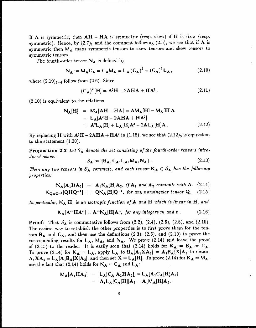
If A is symmetric, then AH - HA is symmetric (resp. skew) if H is skew (resp.

symmetric). Hence, by (2.7), and the commncnt following (2.5), we see that if A is

symmetric then "A maps symmetric tensors to skew tensors and skew tensors tosymmetric tensors.

"The fourth-order tensor NA is defined by

NA MACA = CAMA = LA (CA) 2 = (CA) 2 LA, (2.10)

where (2.10)2-4 follow from (2.6). Since

(CA) 2 [H] = A2H - 2AHA + HA2 , (2.11)

(2.10) is equivalent to the relations

NA[H] = MA[AH - HA] = AMA[H] - MA[H]A

= LA[A 2 7i - 2AHA + HA 2 ]

= A2LA[H] + LA[H]A 2 - 2ALA[H]A. (2.12)

By replacing H with A2H- 2AHA + HA2 in (1.18), we see that (2.12)3 is equivalent

to the statement (1.20).

Proposition 2.2 Let SA denote the set consisting of the fourth-order tensors intro-

duced above:SA := {BA, CA, LA, MA, NA). (2.13)

Then any two tensors in SA commute, and each tensor KA E SA has the following

properties:

KA[AII-A2] = AIKA[H]A 2 , if A1 and A 2 commute with A, (2.14)

KQAQ-1[QHQ- 1 ] = QKA[H]Q-1, for any nonsingular tensor Q. (2.15)

In particular, KA[H] is an isotropic function of A and H which is linear in H, and

KA[A'HA-] = AmKA[H]An, for any integers m and n. (2.16)

Proof: That SA is commutative follows from (2.2), (2.4), (2.6), (2.8), and (2.10).The easiest way to establish the other properties is to first prove them for the ten-

sors BA and CA, and then use the definitions (2.3), (2.6), and (2.10) to prove thecorresponding results for LA, MA, and NA. We prove (2.14) and leave the proofof (2.15) to the reader. It is easily seen that (2.14) holds for KA = BA or CA.

To prove (2.14) for KA = I-A, apply LA to BA[AIXA 2] = AlBA[X]A 2 to obtain

A 1XA 2 = LA[A1BA[X]A 2], and then set X = LA[H]. To prove (2.14) for KA = MA,

use the fact that (2.14) holds for KA =ý CA and LA:

MkA[AIHA 2] = LA[CA[AIHA 2]] = LA[AICA[HIA 2]

= AjLA[CA[H]]A 2 = AjMA[H]A 2 .

8

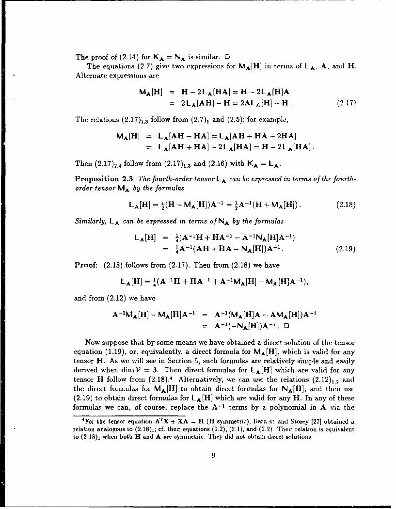
The proof of (2.14) for KA = NA is similar. 0The equations (2.7) give two expressions for MA[It] in terms of LA, A, and IH.

Alternate expressions are

MA[H] = H-2LA[HAI=H-2LA[H]A

= 2LA[AH] -- H = 2ALA,[H] -- H. (2.17)

The relations (2.17)1,3 follow from (2.7), and (2.5); for exanple,

MA[HI = LA[AH - HA] = LA[AHl + HA -- 2HA]

= LA[AH + HA]- 2LA[HA] = H- 2LA[HA].

Then (2.17)2,4 follow from (2.17)1,3 and (2.16) with KA = LA.

Proposition 2.3 The fourth-order tensor LA can be expressed in terms of the fovrth-order tensor MA by the formulas

LA[H] = L(H - MA[H])A.-= !-A-' (H + MA[H]). (2.18)

Similarly, LA can be expressed in terms of NA by the formulas

LA[H] = !(A-'H + HA-1 - A-'NA[H]A-1)= I-A-1(AH +HA - NA[H])A-1. (2.19)

Proof: (2.18) follows from '2.17). Then from (2.18) we have

LA[H] = ¼(A-'H + HA-' + A-IMA[H] - MA [H]A"'),

and from (2.12) we have

A-1MA[II]-- MA[H]A-1 = A~'(MA[H]A- AMA[H])A-1= A-'(-NA[HI)A-'. 0

Now suppose that by some means we have obtained a direct solution of the tensorequation (1.19), or, equivalently, a direct formula for MA[H], which is valid for anytensor H. As we will see in Section 5, such formulas are relatively simple and easilyderived when dirnV = 3. Then direct formulas for LA[H] which are vaid for anytensor H follow from (2.18).4 Alternatively, we can use the relations (2.12)1,2 andthe direct forr.ulas for MA&[H] to obtain direct formulas for NA[Il], and then use(2.19) to obtain direct formulas for LA[H] which are valid for any H. In any of theseformulas we can, of course. replace the A-' terms by a polynomial in A via the

"4For the tensor equation ATX + XA = H (H symmetric), BarnAt and Storey [27] obtained arelation analogous to (2 .18 )1; cf. their equations (1.2), (2.1), and (2.2). Their relation is equivalentto (2.18), when both H and A are symmetric. They did not obtain direct solutions.

9

Cayley-Hamiltou theorem. These techniques will be used iM Sec'ion ý; to gen:ratedirect formulas for LA[H] iin three dimensions.

By (1.18) with H --+ f(A,H), the unique solution X of the tensor efquationAX + XA = *(AH) is given by X = LAJO(A, H)]. If O(A, H) is an isotroplicfunction of A and H which is linear in H (in particular, if #(A, H) has one of theforms in (1.13), (1.21), or (1.22)), then by (2.15) it follows that X is also an isotropicfunction of A and H which is linear in H. When *(A, H) = AH -- HA, this solutioncan also be written as X = MA[Hj. As we will see in Section 5, for arbitrary H thedirect formulas for MA[H] are much simpler than the direct formulas for LA[H], whichshould not be too surprising in view of the method described above for generatingthe latter formulas. For other functions *(A,H) in the list (1.13), the existenceof relatively simple direct formulas for X is due to the fact that there are simpleexpressions for LA[4ý(A,H)] in terms of MARHI, MA[sym H], or NA[H]. We derivethese identities below. Similar results hold for 4(A, H) of the form (1.21) and (1.22);cf. Scheidler [18].

Consider the case 4(A, H) = AHA, i.e., the tensor equation

AX + XA = AHA. (2.20)

Alternate expressions for the solution X = LA[AHA] are given by the followingidentities:

LA[AHA] = ALA[H]A = LA-i[H]

= ½A(H .- MA[H]) = ½(H + MA[H])A

= 4(AH + HA- NA[H]). (2.21)

(2.21)1 follows from (2.16); then (2.21)3,4,5 follow from (2.18) and (2.19)2. To obtain(2.21)2, observe *hat (2.20) is equivalent to the tensor equation

A- 1X + XA-1 = H, (2.22)

and that the solution of (2.22) is X = I-A-' [H]. For A E Psym and H E Sym, rela-tions equivalent to some of those in (2.21) were observed by Mehrabadi and Nemat-Nasser [11]5 and Cohen and Muncaster [24, Ch. 6].6 Our derivations above and in

5in their analysis of the tensor equation (1.9)2 for LI, Mehrabadi and Nemat-Nasser obtainedrelations which, for symmetric A and H, are equivalent to the relations LA-, [HA = ½(H + MA [H])Aand LA-I [H] = ¼(AH + HA -NA [H]); cf. equations (8.8), (8.12), (8.13), and (8.16) in their paper.They also derived a direct formula for MAT[H in three dimensions and used this formula, togetherwith the latter of the two relations above, to obtain a direct solution of (1.9)2; cf. (6.12), in thispaper, which we will obtain by essentially the same technique. However, our derivation of directformulas for MA[H] in Section 5 differs substantially from the method used in [11].

6Cohen and Muncumter considered a tensor equation of the form A-X + XA- 1 + c(tr X)A- 1

G, where A E Psym is the referential Euler tensor and G is symmetric. This equation arises in

10

the next paragraph differ from theirs; in particular, we do not rely on the symmetryof A or H.

Compared with (2.21)2, the formula for MA-1 in terms of MA is much simpler:

MA-1 = -MA. (2.23)

Indeed, from (1.19) we see that X = MA[H] iff A-'X+XA-' = A' (-H)--(-H)A-if" X = MA-, [-H]. Note that some of the identities in (2.21) can also be obtainedby replacing A with A-' in (2.18) and (2.19) and then using (2.23) and (2.12).

For the case 4i(A, H) = A2H + HA2 , we have the identities

LA[A 2H + HA2] = A2LA[H] + LA[H]A 2

= 2LA[H]A2 + AH- HA = 2A 2 LA[H]- AH + HA

= AlH - MA[H]A = HA + AMA[H]

= 1(AH + HA +NA[HI). (2.24)

(2.24), follows from (2.16); then (2.24)2,3 follow from (2.9). (2.24)4,5 follow from(2.24)2,3 and (2.18). Finally, (2.24)6 follows from (2.12)4 and (2.21)5, or from (2.24)4,5and (2.12). Next, consider the case @(A, H) = A2HT+ HA2 . By applying LA to theidentity

A'HT+ HA2 = A2(sym H) + (sym H)A2 + A2(-skw H) - (-skw H)AF

and then using (2.9) with H -+ -skw H, we obtain the identity

LA[A 2HT+ HA 2 ] = LA[A 2(symH) + (symH)A2 ]

+ (skw H)A - A(skw H). (2.25)

Alternate expressions for LA[A 2HT + HA2] follow from this and (2.24) with H --

sym H. In particular, we have

LA[A 2HT + HA2 ] + A(skw H) - (skw H)A

= A(symH) - MA[symH]A =(symH)A + AMA[symH]

= ½(A(symH) + (symH)A + NA[symH]). (2.26)

Finally, for the case k(A, H) = HA - AHT, we have the identity

LA[HA - AHr] = skwH -- MA [sym H]. (2.27)

the analysis of gyroscopic motions of pseudo-rigid elastic bodies. On multiplying this equation byA and taking the trace of the result we may solve for tr X and reduce the original equation to theform (2.22) with H = G- c(2 + 3c)-'tr (GA). Then their equations (6.3.12), (6.3.14), and (6.3.16)are equivalent to our relation LA-, [H] = 1(H + MA[H])A. They did not obtain direct formulas forMA[H] or LA-, [H].

11

This follows from the identity

HA - AHT = -A(sym H) + (symH)A + A(skw H) + (skw H)A,

(2.5) with H --, skw H, and (2.7), with H --+ sym H.We conclude this section with a result mentioned in the introduc ion in connection

with Liapunov functions for systems of differential equations.

Proposition 2.4 The tensor equation ATY + YA = G has a unique solution Y forany given G iff A E Lin*. If A E Lin*, then X = Cm,,ne,nA, HAn is a generaldirect solution of AX + XA = H iff Y = Z,,,, cm,,(A T )' GA- is a general direcrsolution of ATY + YA = G. Here m and n are integers, the sums are assumed to befinite, and the coefficients c,,n may depend on A but not on H or G.

Proof: We use the well-known fact that AT and A are similar, i.e., there is anonsingular tensor S such that AT = SAS- 1 . Let Y = SX and G = SH. Then theequations AX + XA = H and ATY + YA = G are equivalent, and the results of theproposition follow. 0

Since AX + XA = H iff X = LA[H], Proposition 2.4 can be used to transformthe general direct formulas (5.6) and (5.17)-(5.20) for LA[HI in three dimensions intogeneral direct solutions Y of ATY + YA = G. This proposition cannot be appliedto the general direct formulas (5.22), (5.28), and (5.33) since some of the coefficientsin these formulas depend on H.7

3 Some tensor identities in three dimensions

The derivations of the results in Sections 4-7 utilize various identities involvingone or two second-order tensors and their principal invariants. For convenience wehave collected most of these identities in the present section. With the exception ofsome comments at the end of Section 4, for the remainder of this paper we assume thatthe underlying inner product space V is three-dimensional. Unless specified otherwise,the tensors A and H are arbitrary.

The principal invariants of A are denoted by 1 A, HA, and Hll, and its charac-teristic roots (in the complex field) are denoted by a,, a2, a3 . Then

3

det (xI- A)= X 3 - Ax2 + IAX- IIIA = (x-a,), (3.1)i=i

'If in Proposition 2.4 we allowed the coefficients Cm,n in the formula for X to depend on H,say cm., = 6m,(A, H), then since H = S-IG it follows that the coefficients in the correspondingformula for Y would depend not only on A and G but also on the tensor S in the similaritytransformation AT = SAS-'.

12

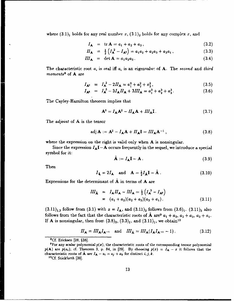
where (3.1), holds for any real number x, (3.1)2 holds for any complex x, and

1A = tr A = a, + a 2 + a 3 , (3.2)

"IIA = 12 (1A IA2) = aja 2 + a2a3 + a3aa, (3.3)

"HIA = det A =aIa2a3 . (3.4)

The characteristic root aj is real iff aj is an eigenvaluc of A. The second and thirdmoments8 of A are

IA2 = I2-21A=a2 + a2+ a, (3.5)IA3 = IA3 - HAMA~ + MIA = a3a + a3 + a. 336

The Cayley-Hamilton theorem implies that

A3 = IAA 2 - IIAA + INA'I. (3.7)

The adjoint of A is the tensor

adj A := A2 - IA + IIAI = IIIA- 1 , (3.8)

where the expression on the right is valid only when A is nonsingular.Since the expression IxA -A occurs frequently in the sequel, we introduce a special

symbol for it:

A := IA'- A. (3.9)

Then

Ik, = 21 A and A = IAI-Al . (3.10)

Expressions for the determinant of A in terms of A are"A = IA ITA - I"-A ( - IA)

= (a, + a2 )(a 2 + a3)(a 3 + a). (3.11)

(3.11)1,3 follow from (3.1) with x = IA, and (3.11)2 follows from (3.6)1. (3.11)3 alsofollows from the fact that the characteristic roots of A are 9 a, + a 2, a 2 + a3 , a3 + a,.If A is nonsingular, then from (3.8)2, (3.3)1, and (3.11)1, we obtain10

"HA = IIAIA-, and III"' = IIIA(IAIA-, - 1). (3.12)

'Cf. Ericksen [28, §38].9 For any scalar polynomial p(x), the characteristic roots of the corresponding tensor polynomial

p(A) are p(a,); cf. Theorem 3, p. 84, in [29]. By choosing p(x) = IA - ax it follows that thecharacteristic roots of AL are IA - ai = a1 + ak for distinct ij, k.

'0 Cf. Stickforth [30].

13

Expressions for the second principal invariant t, A in terms of A are"IIA = 1+IA (31A - IA,) = IA, + 3VIA

- (a, + a2)(a 2 + a3 ) + (a2 + a3 )(a3 + a 1 ) + (a3 + a,)(a1 + a 2). (3.13)

By replacing A with A in (3.8) azd using (3.9), (3.10)1, and (3.13)1, we obtain thefollowing expressions for the adjoint of A:

adj i = A2 + II"I = IIIAA-, (3.14)

where the expression on the right is valid only when A is nonsingular. 11 Let

AA I' -IA = IA2 +IIA=', ~(IA'+IA2) = 'IA.'

- j[(a, + a 2)2 + (a 2 + a3 )2 + (a3 + al)2]. (3.15)

This invariant appears in the direct solution (1.16) of Sidoroff and Guo and also inseveral other formulas in the sequel. Observe that 2 AA is the second moment of .

The following identities are due to Rivlin [17]:

A2HA2 = IIAAHA - IIIA(AH + HA)

+ IA2HA 2 + aA•HA + IIIAIAHI. (3.16)A2HA + AHA2 = IAAHA - IIIAH(2 +A+ HII .IH, (3.17)

+ IAHA 2 + aAHA+"AH (.7

A2H + HA2 + AHA = IA(AH + HA) - IIAH(A 1 ) A+ ci~) 1,(318

+ IH' + A2 H A ,H (3.18)

where

a( ,)= IIIA IH -- IIAIAH IAA2 H (3.19)'AA,H = I2 A- I.IAH = -IAAH, (3.20)

~AH = IA IAIH = -IAH (3.21)

S= A2 - IAIAH + "IAH = I(.djA)H (3.22)

The first expressions in (3.19)-(3.22) are the ones given by Rivlin [17]; the secondexpressions follow easily from these and (3.7)-(3.9). From (3.9), (3.15)1, and (3.18),we obtain the identities

AHHA = AHA - IA(AH + HA) + I21-, a(1) A+ a(°) 1. (3.23)-(A 2H + HA2) + AAH + IAL2 + A,H + A,!H.

"1 The identities (3.10), (3.11)1, (3.13)1, and (3.14)2 were observed by Guo [8]. Various authorshave observed one or both of the identities (3.11)1,3, often unier the assumption that A E Psym.

14

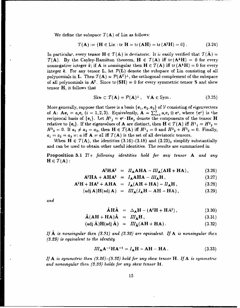
We define the subspace T(A) of Lin as follows:

'T(A) {H E Lin: tr H = tr (AH) = tr (A2 H) - 0}. (3.24)

In particular. every tensor H E T(A) is deviatoric, It ih easily verified that T(A) =T(A). By the Cayley-Hamilton theorem, H E T(A) iff tr(AkH) = 0 for everynonnegative integer k; if A is nonsingular then H E T(A) iff tr (AkH) = 0 for everyinteger k. For any tensor L, let P(L) denote the suibspace of Lin consisting of allpolynomials in L. Then T(A) = 7P(AT)'-, the orthogonal complement of the subspaceof all polynomials in AT. Since tr (SH) = 0 for every symmetric tensor S and skewtensor H, it follows that

Skv c T(A) = P(A)-L, VA E Sym. (3.25)

More generally, suppose that there is a basis {ej, e2, e3 } of V consisting of eigenvectorsof A: Ae, = ajej (i = 1,2,3). Equivalently, A = a;e1 ® ei, where {ei} is thereciprocal basis of {e,1. Let Hij = ei. Ilej denote the components of the tensor Hrelative to {ei}. If the eigenvalues of A are distinct, then H e T(A) iff Hi1 = H22 =

H3 = 0. If a1 :/ a 2 = a 3 , then H E T(A) iff H11 = 0 and H122 +H33 = 0. Finally,a, = a2 = a3 =: a iff A = al iff T(A) is the set of all deviatoric tensors.

When H E T(A), the identities (3.16)-(3.18) and (3.23)2 simplify substantiallyand can be used to obtain other useful identities. The results are summarized in

Proposition 3.1 Ti e following identities hold for any tensor A and anyH E T(A):

A2HA 2 = IIAAHA - IIIA(AH + HA), (3.26)

A2HA + AHA2 = IAAHA - IIIAH, (3.27)

A2H + HA2 + AHA = IA(AH + HA) - IIAH, (3.28)

(adj A)H(adj A) = IIIA(IAH - AH - HA), (3.29)

and

AHA = AH - (AH + HAF), (3.30)

,A(AH+HA)Ak = fIIH, (3.31)

(adj A)H(adj A) = IIIX(AH + HA). (3,32)

If A is nonsingular then (3.31) and (3.32) are equivalent. If A is nonsingular then(3.29) is equivalent to the identity

IIIAA- 1 HA-' = IAH - AH - HA. (3.33)

If A is symmetric then (3.26)-(3.32) hold for any skew tensor H. If A is symmetricand nonstngular then (3.33) holds for any skew tensor H.

15

Proof: (3.26)-(3.28) and (3.30) follow immediately from (3.16)-(3.23) and the defi-nition of T(A). Then (3.8) and (3.26)-(3.28) yield (3.29) and (3.33). To prove (3.31),replace H with AH + HA in (3.23), and use (3.27), (3.28), and (3.11)1. Similarly,(3.32) follows from (3.14)1, (3.26), (3.28), and (3.11)1. Since T(A) = T(A), (3.32)can also be obtained by replacing A with A in (3.29) and using (3.9) and (3 .10)1. If"A is nonsingular then adj A, = IIIAA- 1, in which case (3.31) and (3.32) are easilyseen to be equivalent. The statements for symmetric A follow from these results and(3.25). 0

The identity (3.31) is the key to our construction of simple direct formulas forLA[H] when H E T(A).1 2 Note that since tr(Ak(A'HAn)) = tr(Ak+m+nH), forany nonnegative integers m and n we have

A"HAn -A"HA" ET(A), VA,HE Lin; (3.34)

and if F E T(A) then any linear combination of terms of the form AmHAn belongsto T(A). In particular, for H E T(A) each of the expressions in Proposition 3.1belongs to T(A). We conclude this section with a result which will be utilized in theproof of Theorem 4.1.

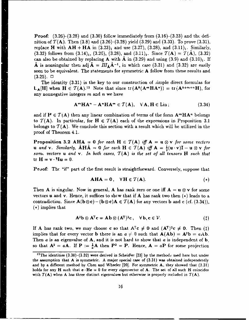
Proposition 3.2 AHA = 0 for each H E T(A) iff A = u 0 v for some vectcrsu andY. Similarly, AHA = 0 for each H E T(A) iff A = 1(u.v)I- u 9v forsomL vectors u and v. In both cases, T(A) is the set of all tensors H such thattr H = v.Hu = 0.

Proof: The "if" part of the first result is straightforward. Conversely, suppose that

AHA = 0, VH E T(A). (H)

Then A is singular. Now in general, A has rank zero or one iff A = u 9 v for somevectors u and v. Hence, it suffices to show that if A has rank two then (*) leads to acontradiction. Since A(b®c)- (b®c)A E T(A) for any vectors b and c (cf. (3.34)),(*) implies that

A2b ®ATc=Ab®(AT)2c, Vb,cEV. (M)

If A has rank two, we may choose c so that ATc # 0 and (AT) 2c # 0. Then (t)implies that for every vector b there is an a 7/ 0 such that A(Ab) = A2b = aAb.Then a is an eigenvalue of A, and it is not hard to show that a is independent of b,so that A2 = aA. If P := IA then p2 = P. Hence, A = aP for some projection

12The identities (3.30)--(3.32) were derived in Scheidler (23] by the method.s u&ed here but underthe assumption that A is symmetric. A major special case of (3.31) was obtained independentlyand by a different method by Chen and Wheeler [20]. For symmetric A, they showed that (3.31)holds for any H such that e He = 0 for every eigenvectot of A. The set of all such H coincideswith T(A) when A has three distinct eigenvalues but otherwise is properly included in T(A).

16

P of rank two. Then there is a basis {ei} of V with reciprocal basis {ei} such thatP = e 2 ® e2 + e3 ® e 3, in which case (*) implies that H 2

2 = H33 = H 2

3 = H32 = 0for each H E T(A). But from the comments preceding Proposition 3.1, we see that

H E T(A) if H 11 = 0 and H22 = -H 3

3 -# 0, which is a contradiction. Finally, notethat since T(A) = T(A) for any tensor A, we have AHA = 0 for each H e T(A) iff

AHA = 0 for each H E T(A) iff A = u®v iff (cf. (3.10)) A = !(u.v)I- u0v. 0

4 Existence and uniqueness of solutions.Direct solutions in T(A)

Here, as in the previous section, we do not require that A E Lin*, i.e., that theequation AX + XA = H has a unique solution X for every H E Lin. Instead, inTheorem 4.1 and Proposition 4.2 we determine necessary and sufficient conditions forthe existence of a unique solution as well as simple direct formulas for this solutionwhen X and H are restricted to the subspace 'T(A). These results are then used in the

proof of Theorem 4.2, which gives necessary an2d sufficient conditions for A E Lin*.We begin with the following result which is utilized in the proofs.

Proposition 4.1 If X E T(A) then AX + XA e T(A); i.e. B_ maps T(A) into

itself. Conversely, if A is nonsingular and AX + XA E T(A), then X E T(A). Inparticular, kerBA C T(A) if A is na)nsi-tgular.

Proof: The first part is jnst a special case of the result stated after (3.34). Con-versely, suppose that A is nonsingular and AX + XA E 'T(A). Then

2tr(Ak+IX) = tr(Ak (AX + XA)) = 0 for any integer k, so that X E T(A).13

Finally, X E ker RA iff AX + XA = 0 E 1(A). 0

Theorem 4.1 The following conditions are equivalent:

(1) M, :A 0;(2) The restriction of BA to the subspace T(A) is nonsingular;(3) For each H c T(A), the equation AX + XA = H has exactly one solution

X E T(A) (the possibility of other solutions outside of the subspace T(A) isnot excluded).

When 111A # 0, direct formulas for the solution X E T(A) are

IIIAX = AHW = AHA - IA(AH + HA) + IAH= AAH- (A2H + HA2). (4.1)

If A is symmetric with IllA # 0 and if H is skew, then (4.1) is the only skew soluiionofAX + XA = H.

"I1f we dropped the assumption that A is nonsingular then we could only conclude thattr(Ak+IX) = 0 holds for nonnegative k, which does not imply trX = 0.

17

Proof: From the first part of Proposition 4.1, we see that (2)€€(3). From (3.31)with H --4 X, we have

.AA[XIA = A(AX + XA)A = 1IIX., VX E T(A). (*)

If II'A j4 0, then by (*) it follows that the conditions X E 'T(A) and BA[X] = 0 imply

X = 0. Hence, (1)=ý-(2)€•(3); and (3), together with (*), implies AHA = IIIAX, i.e.,(4.1)1. Then (4.1)2,3 follow from (3.23), and (3.30). If A is symmetric and H is skewthen AHAk is skew. Since Skw C T(A), and since (4.1) is the only solution in T(A),it follows that (4.1) is the only solution in Skw. It remains to show that (3) implies(1). Suppose that (3) holds and that I"iA = 0. Then by (*), it follows that AHA = 0for each H E T(A). Hence, by Preposition 3.2, we must have A - 2(u. v)I- u 0 vfor some vectors u and v, in which case H E T(A) iff tr H = v Hu = 0. Butthen for any vector w orthogonal to u, the tensor H := u 0 w belongs to T(A) andsatisfies AH + HA = 0, wbich contradicts (3). Hence III, must be nonzero. C1

Recalling the definition (3.15) of AA, we see that (4.1)3 is the direct solution (1.16)obtained by Sidoroff [6] and Guo [8] under the assumptions A E Psym and H E Skw.Various necessary and sufficient conditions for III"• A 0 follow from the results in theprevious section and are summarized in

Proposition 4.2 The following conditions are equivalent:

(1) IxI #0; (2) A is nonsingular;(3) IAIIA # "'A; (4) I' # IA,;

(5) 1A is not an eigenvalue of A; (6) a, + a, # 0, Vi # j E {1,2,3}.

Since any nonreal characteristic roots of A occur in a complex conjugate pair, from(6) we see that if A has a characteristic root with nonzero real and imaginary partsthen III,& # 0. Also note that A may be nonsingular even if A is singular. Indeed,from (6) we see that the conditions

a,=0, a2 #0, a3 #0, a2 +a 3 #0 (4.2)

are sufficient for III' # 0, and that if a, = 0 then the other conditions in (4.2) arenecessary for IIIA # 0. It follows that if A is nonsingular then the null space of Ahas dimension at most one.

By combining the above results, we obtain

Theorem 4.2 The following conditions are equivalent:

(1) A E Lin'; (2) A and A are nonsingular;(3 ) IIIA# 0 and IIIA # 0; (4) IAIIA# IIIA # 0;(5) IMlA#OandlAIA-, I#; (6) a,+ajO0, Vi,jE{1.2,3};(7) neither 0 nor IA is an eigenvalue of A.

18

Proof: The equivalence of (2)-(7) follows from Proposition 4.2 and (3.12)2. That (1)implies (2) follows from Proposition 2.1 and Theorem 4.1. Conversely, if (2) holds thenby Proposition 4.1 and Theorem 4.1 we have ker BA C T(A) and ker BAnT(A) = {0},respectively. Hence, kerBA = {0}. 0

From (4) of Theorem 4.2 we see that A E Lin* if A is nonsingular and deviatoric.From (6) we see that A E Lin* if the characteristic roots of A have positive real parts(e.g., A E Psym), or if the characteristic roots of A have negative real parts (e.g.,-A E Psym), or if A has a nonzero eigenvalue and a characteristic root with nonzeroreal and imaginary parts.

The only part of Theorem 4.2 that carries over (with obvious modifications) toarbitrary dimensions is the equivalence of (1) and (6). This result is a special case of

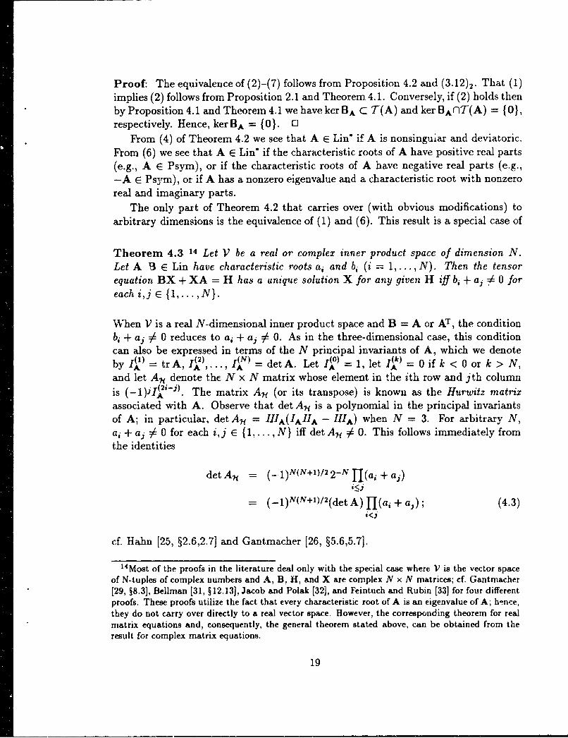
Theorem 4.3 14 Let V be a real or complex inner product space of dimension N.Let A 3 E Lin have characteristic roots ai and bi (i = 1,...,N). Then the tensorequation BX + XA = H has a unique solution X for any given H iff bi + aj : 0 foreach i,j E {1,...,N}.

When V is a real N-dimensional inner product space and B = A or AT, the conditionbi + aj $ 0 reduces to a, + aj $ 0. As in the three-dimensional case, this conditioncan also be expressed in terms of the N principal invariants of A, which we denoteby I(')= trA, I('),... I(N)= detA. Let 1"0) -1, let I)= 0 if k <0 or k > N,

and let AH denote the N x N matrix whose element in the ith row and jth columnis (-1)'I('-j. The matrix A,. (or its transpose) is known as the Hurwitz matrixassociated with A. Observe that det An is a polynomial in the principal invariantsof A; in particular, det AH = IIIA(IAIIA - IIIA) when N = 3. For arbitrary N,a, 4- aj ' 0 for each i,j E {1,...,N} iff det AH # 0. This follows immediately fromthe identities

detA, = (.-1)N(N+i)/22-N]J(a, +aj)

- (-1)N(N++)/ 2(detA) ]J(aj+a,); (4.3)i<j

cf. Hahn [25, §2.6,2.7] and Gantmacher [26, §5.6,5.7].

"1 4Most of the proofs in the literature deal only with the special case where V is the vector spaceof N-tuples of complex numbers and A, B, 11, and X are complex N x N matrices; cf. Gantmacher[29, §8.3], Bellman [31, §12.13], Jacob and Polak [32], and Feintuch and Rubin [33] for four differentproofs. These proofs utilize the fact that every characteristic root of A is an eigenvalue of A; hence,they do not carry over directly to a real vector space. However, the corresponding theorem for realmatrix equations and, consequently, the general theorem stated above, can be obtained from theresult for complex matrix equations.

19

5 Direct formulas for LA, MA, and NA

in three dimensions

In this section we assume t,.ai A E Lirt* and V is three-dimensional. Then fromTheorem 4.1 and (1.18) it follos :hi•,t for each H E T(A),

IlIA-A[k!] = AHA

= AHA - IA(AH + HA) + I2H

= AAH- (A 2H + HA2 ); (5.1)

in particular, these formulas hold whenever ±A E Psym and H E Skw, in which caseLA[H] is skew. For arbitrary H, all of the direct formulas for LA[H], MA[H], andNA[H] derived below will be obtained from (5.1)1,2, the results in Sections 2 and 3,and the fact that AH - HA E T(A) for each A, H E Lin, which is just a special caseof (3.34). This last fact allows us to replace H with AH - HA in (5.1).

By replacing H with AH - HA in (5.1), and using MA['T] = LA[AH - HA] andA = IAI - A, we obtain

III hMA[H] -. A(AH- HA)A = A(H. - .H)A= A(AHA) - (AHA)A = (AHA)A - A(AHA)

= AHj 2 - 2Hk (5.2)

for any tensor H. Similarly, from (5.1)2 with H -+ AH - HA, we obtain

IIIAMA[H] = A2HA - AHA 2 + IA(HA2 - A2H) + IA2(AH - HA). (5.3)

A lengthier derivation of this result follows by replacing H with AH - HA in (5.1),3;this yields some A3 terms which can be reduced by means of the Cayley-Hamiltontheorem (3.7). Mehrabadi and Nemat-Nasser [11] obtained (5.3) by repeated appli-cations of the Cayley-Hamilton theorem.

In view of (1.19), the direct formulas (5.2) and (5.3) yield a variety of directsolutions X = MA [H] of the tensor equation AX+XA = AH-HA, H arbitrary. Inparticular, if A and H are symmetric then MA[H] is skew, and we have the alternateformulas

IIIAMA[H] = 2skw(AiAHA)= 2skw(AHA 2)

= 2skw (A2HA - IA2H + IA2AH) (5.4)

and

-IIlAtfl1[H] = 2skw(AHAA)= 2skw(A 2HA)

= 2skw (AHA2 - IAHA2 + I2HA) (5.5)

20

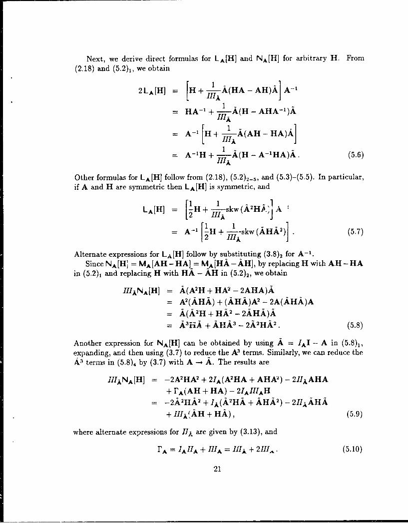
Next, we derive direct formulas for LA[H] and NA[It] for arbitrary H. From(2.18) and (5.2)1, we obtain

2LA[H] = [H + -A,(HA - AH)AJ A-'"'IA

= HA-' + +/--A(H - AHA-1)A

= A-' [H + 1"iA H - HA)A]

= A-'H + +-A(H - A--'HA)A. (5.6)

Other formulas for LA[H] follow from (2.18), (5.2)2-5, and (5.3)-(5.5). In particular,if A and H are symmetric then LA[H] is symmetric, and

L1] H + 1!skw(A 2Hj., A I

=A,-' 1 + "-Askw(kHA2) (5.7)

Alternate expressions for LA[H] follow by substituting (3.8)2 for A-'.Since NA[H] = MA[AH- HA] = MA[HA- AH], by replacing H with AH- HA

in (5.2), and replacing H with HA - AH in (5.2)2, we obtain

IIIANA[H] = A(A 2H + HA2 - 2AHA)A= A2(AHA) + (AHA)A 2 - 2A(AHA)A= A(A 21 + HA 2 - 2AHA)A= A 3 iA + AHA 3 - 2A 2 HA 2 . (5.8)

Another expression for NA[H] can be obtained by using A = ,IA - A in (5.8)1,expanding, and then using (3.7) to reduce the A3 terms. Similarly, we can reduce theA,3 terms in (5.8)4 by (3.7) with A --+ A. The results are

IIIANA[H] = -2A 2HA 2 + 21A(A 2HA + AHA2 ) - 2IIAHA

+ FA(AH + HA) - 2 IAIIIAH= -2. 21HA 2 + IA(A 2HA + AHA 2 ) - 21IAAHA

+ IIIAtAH + HA), (5.9)

where alternate expressions for II, are given by (3.13), and

FA = IAIIA + IIA = 11IA + 21II1,. (5.10)

21

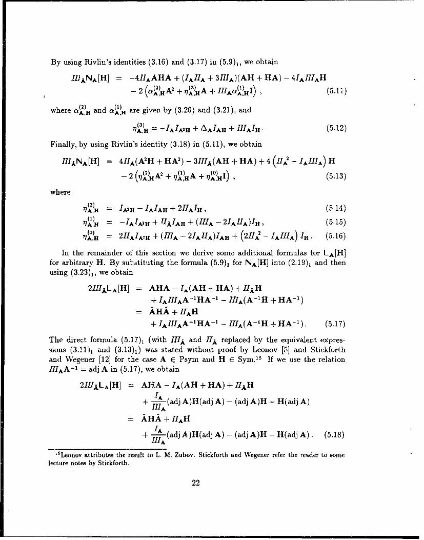
By using Rivlin's identities (3.16) and (3.17) in (5.9)1, we obtain

IIDANA[H] = -4IIAAHA + (IAIIA + 3111A)(AH + HA) - 4 IAIIIAII-2 (a(�()A2 + A "'A1A HI)7 (5.11)

where a(2) and al), are given by (3.20) and (3.21), and

*7A = IA/ + AAIAH + "'AIH. (5.12)

Finally, by using Rivlin's identity (3.18) in (5.11), we obtain

IIIAkNA[H] = 411A(A 2H + HA2) - 3I1IA(AH + HA) + 4 (IIA2 - IAIIIA) H(2 2+q(1) A " 0 (5.13)

where

7(2) 1 A2 -- IAIAH + 2 11AIH, (5.14)

(71) = -IAIA2 H+ TIAIAH +(IIIA- 2IAIIA)IH, (5.15)0) - 2 IIAIA2H + (IIIA - 2 IAIIA)IAH + (2II1A - IAIIIA) 'H (5.16)

7A,H -

In the remainder of this section we derive some additional formulas for LA[H]for arbitrary H. By sutstituting the formula (5.9), for NA[H] into (2.19), and thenusing (3.23)1, we obtain

211IALA[H] = AHA - IA(AH + HA) + IIAH

+ IAIIIAA-I HA-1 - IIIA(A- 1 H + HA- 1 )= AHA + IIAH

+ IAIIIAA,-HA- 1 - IIIA(A-'H + HA- 1 ). (5.17)

The direct formula (5.17), (with If'A and Ilj replaced by the equivalent expres-

sions (3.11), and (3.13)1) was stated without proof by Leonov [5] and Stickforthand Wegener [12] for the case A E Psym and H E Sym.' 5 !f we use the relation

IIIAA-1 = adj A in (5.17), we obtain

211HALA[H] = AHA - IA(AH + HA) + IIAH

+ - (adj A)H(adj A) - (adj A)H - H(adj A)"'IA

= AHA + IIAH

+ I(adj A)H(adj A) - (adj A)H - H(adj A). (5.18)

"t5Leonov attributes the resu!t to L. M. Zubov. Stickforth and Wegener refer the reader to somelecture notes by Stickforth.

22

If the formula (3.8)2 for IIIA-1 is substituted into the last term in (5.17)1, we obtain

2IIILA[H] = AHA - (A 2H + HA2) + AA- + IAIIIA-A HA-1. (5.19)

The formulas (5.18)2 and (5.19) aie due to Mfiller [16] and Jameson [151, respectively.16

By using (3.8) in (5.19) or (5.18), and expanding, we obtain

2IH.AIIIALA[H] = IAA2 HA2 - I12 (A2HA + AHA 2) + III] (A2H + HA2 )

+ (IU + lIA) AHA - I2I[A(AH + HA) + OAH, (5.20)

w here 2 + I I A

w r= IA2IIA + IIAIIII.+ = 1 +IIA

= IIAI + IAIIIA- IAIIIIA . (5.21)

In view of (1.18) and (3.11)1, this is the direct formula (1.17) of ttoger and Carlson[9];17 cf. also Smith [14].11

Substitution of Rivlin's identities (3.16)-(3.18) into (5.20), together with (3.23)1,yields

IIIkLA[H] = AHA - IA(AH + HA) + I2H+#A(2)A2 + /3A()A + Q()I

= A-1iAL + a (2)A2 + 0(l) A + 3(0?H1, (5.22)

where

A(2) (IAIA2H 121AH + IIIAIH) =A TA-1H -TH

- III (-IAIAAH ± II'AIH) = 'AA-'H' (5.23)

l*4Liller and Jameson obtained direct solutions of the tensor equation BX+XA = H for arbitrarydimensions. Muller's formula is quite complicated. For the case B = AT, both authors simplifiedtheir general results, and Jameson listed the corresponding formulas in two and three dimensions.For B = AT and dimV = 3, the formulas of Miller and Jameson are equivalent to those obtainedirom (5.18)2 and (5.19), respectively, via Proposition 2.4; they reduc- to (r I'8)2 and (5.19) whenA is symmetric. Their general formulas (f(r A and P unrela,-d) also reduce to (5.18)2 and (5.19)when B = A.

"17Hoger and Carlson showed that (1.17) is asolution of AX + XA = H for any tensor H and anytensor A such that LVA(IA RA - 'HA) 0 0. They established uniqueness of this solution when A isalso symmetric.

"8 For symmetric H, Smith obtained a direct iolution of the tensor equation ATX + XA = Hfor arbitrary N = iimV. This solution has the form (det AN)X = n=1 cm,n(AT)"where Ali is the Hurwitz matrix associated with A (cf. Section 4), aný the coefficients cm,n arecomplicated polynomials in the principal invariants of A involving cofactors of Aj. Smith gaveexplicit expressions for these coefficients when dimaV z 2,3,4. For dimV = 3, his formula isecuivalent to the one obtained from (1.17) via Proposition 2.4; this formula reduces to (1.17) whenA is symmetric.

23

2PIAH _ m [ H + ('A - liA) XA,, + &3IH]IIIA

-JAH + 21AIH - I'IA-H = IAH - IAIAA.-'H, (5.24)

2/3,H = 'HA (IIIAIA2H + IAIAH + I3AIH)

=-AIAH + "I'AA-,H IIIA(IAI.,2H - IA-IH), (5.25)

and

ý, = IA(IIIA- IIA)A= (2IIA- IAIA), (5.26)

#A = IAH.A - IA II.A = AIA -

= IA 2• I -' IIIAA- IIAIIIA. (5.27)

From (5.22) and (3.23)2, we also have

IIIALA[H] = -(A 2H + HA 2) + AAH+A(2)A2 + •(1)HA + 1(°,)1 (5.28)

where2%) -t A(! 1 (IAIA2i _ IA21AK + -FAIM)

Ilia

1= W- (-IAIAH + FAIH) = 'H + I'AA-H,, (5.29)

2 = A( 7,) 1 [-I2IAH + (IA + IHiA) !AH - IAIIAIH]

= IAH - IA2'A-H = -(IAH + IAIj-LH), (5.30)

2-yA,H 7IA(AAH- IiaIA -AH

=' _IAIAH + rAIA-IH = IIIA(IA-'H + IAIA-2H)., (5.31)

rA is given by (5.10), and

yA = itArA - IA1IIA =IAIIh' - IIIAAA

= IAIIA - IA IIIA + II4IIIA. (5.32)

The direct formula (5.28) with the expressions (5.29)3, (5.30)2, and (5.31)3 for Y( H isdue to Sidoroff [6].19 The direct formula (5.28) with the expressions (5.29)1, (5.30)I,

and (5.31), for ( was obtained by Hoger and Carlson [9] by essentially the samemethod as used here, i.e., from the direct formula (5.20) and Riviin's identities. Hoger

"1For A E Psym, Sidoroff derived (5.1)3 for skew H and (5.28) for symmetric H and then combined

these to obtain (5.28) for arbitrary H. He noted that (5.28) yields a solution of AX + XA = H forany tensor A such that HIIA,(IAHA - Ml-A) $ 0, but did not establish uniqueness for this case.

24

and Carlson observed that (5.28) collapses to the formula (5.1)3 of Sidoroff and Guowhen A E Psyrn and H is skew. Indeed, for any A E Lin* and any (E T(A), we seethat (5.22) and (5.28) collapse to (5.1)1,2 and (5.1)3, respectively. The direct formulas(5.6), (5.7), and (5.17)-(5.20) do not have this property.

From (5.22)2 and the identity A2 = j 2 + 2 IAA - I2I, we obtainIIIXIA[H] = x (H 4 ilHI) A - Y(?HA + b(l) I

(H + #A(2HI) 1)A+ -•- -A, + b I1 (5.33)

where26(o) a (o) = II(

2r(IH -- i--A A,• H AI IA-1. , (5.34)

26(1 _ 1,,A (AIA7H + SAIAH + IIAbAIH)

IAIAH + bA/A-1H, (5.35)

and

S= "IA, =-(IAAA-+ ,A) = -3 (21A + IA), (5.36)

ýA = 1A + ýA = IA(IIIA - A)= IA(IAAA + 2 HIA)

= IA(IA- IIHA + 2IIA). (5.37)

Also, by (5.23) and (5.30), we have

.-AH zA:. A,H + ½'2H. (5.38)

We conclude this section by considering the special case where A and H are

time-dependent tensors with H related to A, its time rate of change A., and some

time-dependent tensor Z as follows:

H =A 4- AZ- ZA; (5.39)

cf. (6.4) and (7.14). Then tr(p(A)H) = tr(p(A)A), where p(A) is any polynomial

in A. In particular, we have

IH = IA '=A Ikn"A ='i., (5.40)

IA H = IAA =2 i]Al I.iA, A- fIA, (5.41)

IA2H = IA2L - A•A 'A'A - VAL, (5.42)

I(adjA)H = I(djA)A = I'A, I-'H = /A-' = IHA/IlA. (5.43)

These identities yield alternate expressions for the coefficients in the direct formulas

(5.22), (5.28), and (5.33) for LA[H] and for the coefficients in the identities (3.16)--

(3.18) and (3.23)2.

25

6 Applications to kinematics of continua

In this section we apply the preceding results to the derivation of some kinematicformulas for a material undergoing a smooth motion in three-dimensional space. Bytaking the material time derivative of the relations U 2 = C and V2 = B, we obtainthe tensor equations (1.6) for U and V. Hence,

UJ=Lu[,C] and Vr=Lv[]B]. (6.1)

A variety of direct formulas for t in terms of (C and U, and for Vr in terms of 1B andV, follow from (6.1) and the direct formulas for LA[H] in Section 5. In particular,the formulas that follow from (5.20) and (5.28) are due to Hoger and Carlson [9].

By differentiating B = FFT and using the relation between the velocity gradientand the material time derivative of the deformation gradient,

F'= LF, (6.2)

we obtain the following formulas for the material time derivatives of B and B-i:

B = LB + BLT and - (B- 1 ) = B- 1 BB-' = B- 1 L + LTB-. (6.3)

Then (6.3), (1.4), and the definition (1.5) of the Jaumann rate yield the tensor equa-tions (1.10) for D. Hence,

D = LB[]N = -LB-1 [(B-')°]. (6.4)

A variety of direct formulas for D in terms of AI and B, or in terms of (B-1 )' and B- 1,follow from (6.4) and the direct formulas for LA[H] in Section 5. In particular, theformulas which follow from (6.4) and (5.17), are due to Leonov [5], and the formulawhich follows from (6.4), and (5.28) is due to Sidoroff [6]. Also note that the identities(5.40)-(5.43) can be used in the expressions for the coefficients in the direct formulasfor D which follow from (6.4), (5.22), (5.28), and (5.33).

Let LR denote the rotated velocity gradient:

LR := RTLR = DR + WR. (6.5)

Here DR and WR denote the rotated stretching and spin tensors:

DR := R T DR = symLR and WR:= RTWR = skw LR. (6.6)

By difft 1entiating C = FTF and using (6.2), (1.4)2, F = RU, and (6.6)1, we obtain

C= 2FTDF = 2UDRU. (6.7)

26

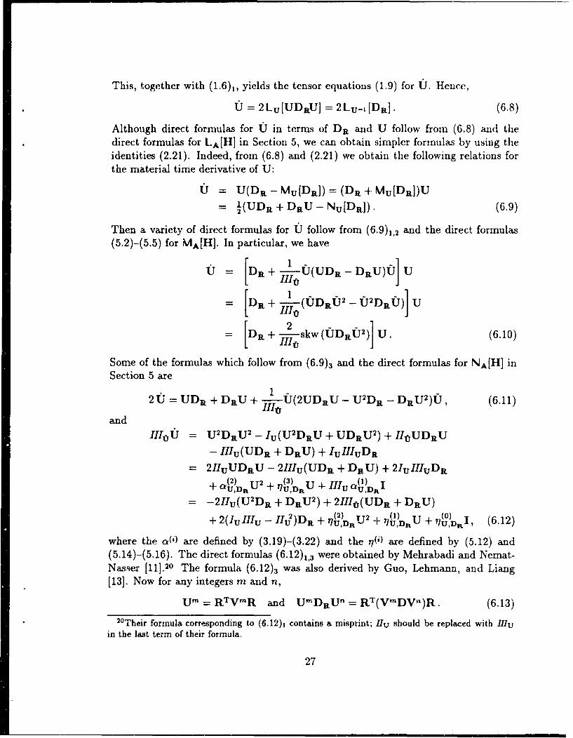
This, together with (1.6),, yields the tensor equations (1.9) for U. Hence,

U0 = 2 Lu [UDRU] = 2 Lu-1 [DR]. (6.8)

Although direct formulas for UJ in terms of DR and U follow from (6.8) and thedirect formulas for LA[HI in Section 5, we can obtain simpler formulas by using theidentities (2.21). Indeed, from (6.8) and (2.21) we obtain the following relations forthe material time derivative of U:

UJ = U(DR - Mu[DR]) = (DR - Mu[DR])U= •(UDR + DRU - Nu[DaI). (6.9)

Then a variety of direct formulas for U follow from (6.9)1,2 and the direct formulas(5.2)-(5.5) for MA[H]. In particular, we have

0 = [DR + -1-V(UDR - DRU)U] U

= [DR+ .1-1(UDRaU2 - f2DRU)] U

= DR + 2Vskw (UDRU2) U. (6.10)

Some of the formulas which follow from (6.9)3 and the direct formulas for NA[H] inSection 5 are

2U = UDR + DRU + I/-- (2UDnU - U 2DR - DtU2)U, (6.11)

andIIIoU = U 2 DRU 2

- IU(U 2DRU + UDRU 2) + IIOUDRU

- IIIu(UDR + DRU) + IuIIIuDR= 211UUDRU - 2111u(UDR + DRU) + 2 1uIIIuDR

+ uv''(2) U,2 (3 rlt! U + IIIu a('), I= UDRU + 77U + "' U,DR 1

= -21Iu(U 2DR + DRU 2) + 2H11D(UDR + DRU).(2) UT2 (1) (

+ 2 (IuIIIu - IIv])DR + "7U,DRU2 + "U,DRU + 77UDýRI1, (6.12)

where the c(i) are defined by (3.19)-(3.22) and the i7(i are defined by (5.12) and(5.14)-(5.16). The direct formulas (6.12)1,3 were obtained by Mehrabadi and Nemat-Nasser [11].20 The formula (6.12)3 was also derived by Guo, Lehmann, and Liang[13]. Now for any integers m and n,

U- = RTV'R and U-DRU" = RT(V-DV-)R. (6.13)2°Their formula corresponding to (6.12), contains a misprint; flu should be replaced with MIu

in the last term of their formula.

27

By use of (6.13) we may convert (6.10)-(6.12) to formuas for U in terms of D, V,and R. When this conversion is applied to (6.12)1, we recover a formula obtained byHoger [10].

From (1.6)2, (6.3)1, and B = V 2 , we obtain the tensor equation (1.7) for V.Hence,

V= Lv[V2LT + LV 2]. (6.14)

Direct formulas for V in terms of L and V follow from (6.14) and the direct formulasfor LA[H] in Section 5; in particular, the formula for V obtained from (5.17), isdue to Stickforth and Wegener [12]. However, simpler formulas can be obtained byusing the identities (2.26). Indeed, from (6.14), (2.26), (1.4), and (1.5), we obtain thefollowing relations for Jaumann rate of V:

0

V = VD- Mv[D]V = DV + VMv[D]

= J(VD+DV+Nv[D]). (6.15)

These relations can also be derived as follows. From (1.7) and (1.4), we have

VVr + VV = V2D + DV2 - V2W + WV2. (6.16)

But this is easily seen to be equivalent to the tensor equation (1.8) for V. Hence,

V = Lv[V 2D + DV 2], and the identities (2.24) yield (6.15). A variety of directformulas for the Jaumarnn rate of V follow from (6.15)1,2 and the direct formulas forMA[H] in Section 5. In particular, we have

III4(V - DV) = VV(VD - DV)V

= V(VDV 2 -V 2D)V)= Vskw (VDV 2). (6.17)

Some of the formulas which follow from (6.15)3 and the direct formulas for NA[H] inSection 5 are

2V = VD + DV + 1 V(V 2 D + DV 2 - 2VDV)V, (6.18)

andIJV 4 = -V 2DV 2 + Iv(V 2DV + VDV2 ) - IIvVDV

+ IvIIv(VD + DV) - IvIIIvD= V 2DV 2 + Iv(V 2DV + V¢DV 2) - IIVVDV + IvIIlIVD

=-2IIvVDV + ('v"Iv + IIIv)(VD + DV) - 2IvIIIvD

?V,D-- -- 1 ,V - Mva() I

= 21v(V2D + DV 2) - IIIV(VD + DV) + 2(IIV - IvHIIv)D(2J ) V 2 _ (1) V ý(•!D I (6.9V,DV- - V,D- VD (6.19)

28

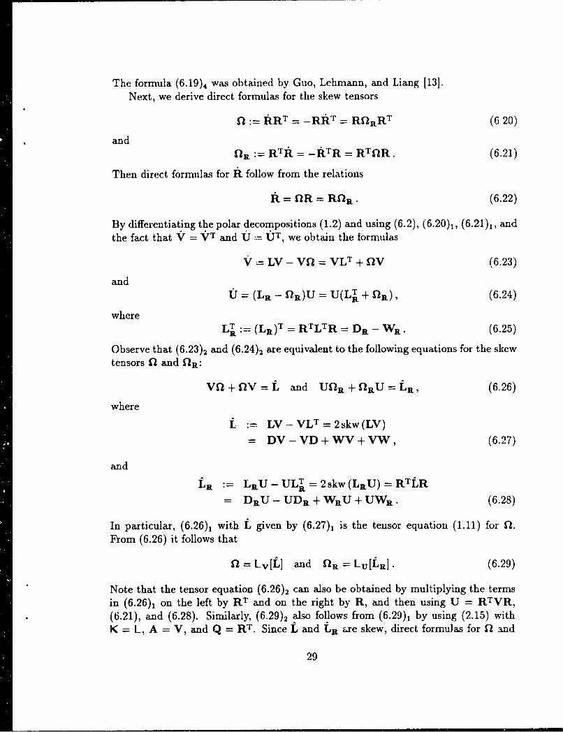
The formula (6.19)4 was obtained by Guo, Lehmann, and Liang [13].Next, we derive direct formulas for the skew tensors

0 := ART= -RRT = RORRT (620)

andOR := RTR = -fRTR = RTOR. (6.21)

Then direct formulas for it follow from the relations

it = OR = R],l. (6.22)

By differentiating the polar decompositions (1.2) and using (6.2), (6.20)1, (6.21)1, andthe fact that V = VrT and U .= UT, we obtain the formulas

V= LV- Vn = VLT + OV (6.23)

andj - (LR - OR)U = U(LT + eR), (6.24)

whereLT (LR)T = RTLTR = DR - WR. (6.25)

Observe that (6.23)2 and (6.24)2 are equivalent to the following equations for the skewtensors 0 and OR:

Vn+nV =L and UnRO+RU=LR, (6.26)

where

L. := LV-VLT=2skw(LV)= DV-VD+WV+VW, (6.27)

and

L4 LU- ULT = 2skw(LRU) =RTLR

= DrU - UDR + WRU + UWR. (6.28)

In particular, (6.26), with 1 given by (6.27), is the tensor equation (1.11) for f.From (6.26) it follows that

12 Lv[L] and OR = Lu[LR]. (6.29)

Note that the tensor equation (6.26)2 can also be obtained by multiplying the termsin (6.26), on the left by RT and on the right by R, and then using U = RTVR,(6.21), and (6.28). Similarly, (6.29)2 also follows from (6.29), by using (2.15) withK = L, A = V, and Q = RT. Since L and LR are skew, direct formuJas for S1 and

29

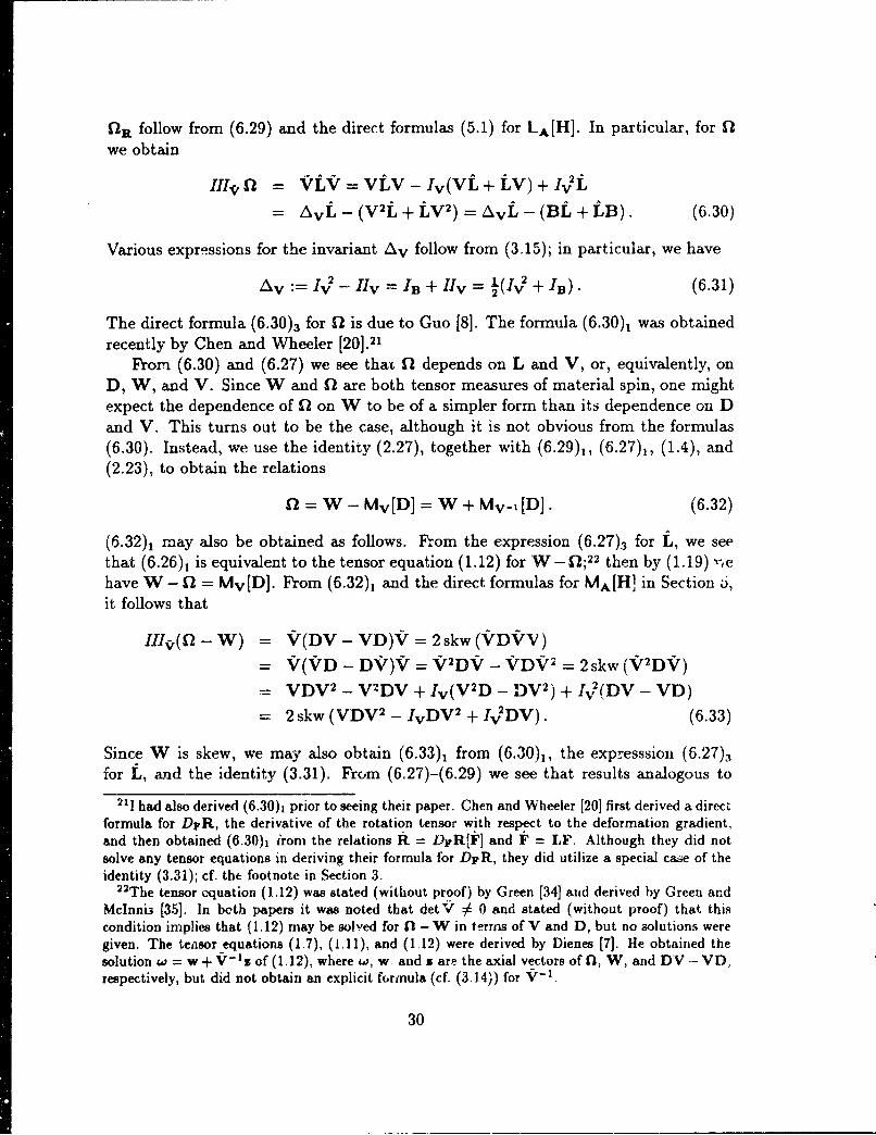
fl] follow from (6.29) and the direct formulas (5.1) for LA[H]. In particular, for f1we obtain

1Ik fn = VLV V=LV - Iv(VL + LV) + IVL

= AV - (V 2 L + LV 2 ) = Avt - (BL + LB). (6.30)

Various expressions for the invariant AV follow from (3.15); in particular, we have

Av := IV- Iv = IB + IIV= .(I + IB). (6.31)

The direct formula (6.30)3 for 11 is due to Guo [8]. The formula (6.30), was obtainedrecently by Chen and Wheeler [20].21

From (6.30) and (6.27) we see that ft depends on L and V, or, equivalently, onD, W, and V. Since W and fl are both tensor measures of material spin, one mightexpect the dependence of f2 on W to be of a simpler form than its dependence on Dand V. This turns out to be the case, although it is not obvious from the formulas(6.30). Instead, we use the identity (2.27), together with (6.29)1, (6.27)1, (1.4), and(2.23), to obtain the relations

fl = W-Mv[D] = W + Mv-i[D]. (6.32)

(6.32), may also be obtained as follows. From the expression (6.27)3 for L, we seethat (6.26), is equivalent to the tensor equation (1.12) for W - Q;22 then by (1.1.9) ",ehave W - 0 = Mv[D]. From (6.32), and the direct formulas for MA[H] in Section 0,it follows that

IIVc(O - W) = V(DV - VD)V = 2skw((VDVV)

= V(VD - DV)V= V 2DV - VDV 2 = 2skw (V 2DV)

= VDV2 - V 2DV + Iv(V 2 D - DV 2 ) + I,;(DV - VD)

= 2skw (VDV2 - IvDV2 + I2DV). (6.33)

Since W is skew, we may also obtain (6.33), from (6.30)j, the expresssion (6.27)3for L, and the identity (3.31). From (6.27)-(6.29) we see that results analogous to

211 had also derived (6.30), prior to seeing their paper. Chen and Wheeler [20] first derived a direct

formula for DFR, the derivative of the rotation tensor with respect to the deformation gradient,and then obtained (6.30), irom the relations R = DFR[F] and F = LF. Although they did notsolve any tensor equations in deriving their formula for DFR, they did utilize a special cabe of theidentity (3.31); cf. the footnote in Section 3.

"12The tensor equation (1.12) was stated (without proof) by Green [34] arid derived by Green andMclnnis [35]. In beth papers it was noted that detV # 0 and stated (without proof) that thiscondition implies that (1.12) may be solved for S) -W in terms of V and D, but no solutions weregiven. The tensor equations (1.7), (1,11), and (1.12) were derived by Dienes [7]. He obtained thesolution w = w + V•-z of (1.12), where w, w and z are the axial vectors of n), W, and DV -- VD,respectively, but did not obtain an explicit fo-rmnula (cf. (3.14)) for V'-

30

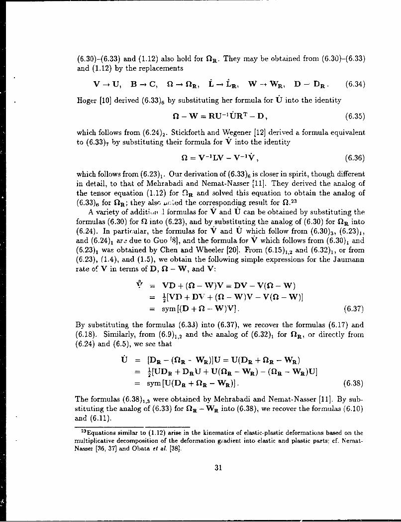
(6.30)-(6.33) and (1.12) also hold for SIR. They may be obtained from (6.30)-(6.33)and (1.12) by the replacements

V -U, B-C, - 1--+ f1R, fL a, W--*WR, D- DR. (6.34)

Hoger [10] derived (6.33)6 by substituting her formula for UJ into the identity

12 - W = RU-1YURT - D, (6.35)

which follows from (6.24)2. Stickforth and Wegener [121 derived a formula equivalentto (6.33)7 by substituting their formula for V into the identity

ft = V-'LV - V-1V, (6.36)

which follows from (6.23)1. Our derivation of (6.33)6 is closer in spirit, though differentin detail, to that of Mehrabadi and Nemat-Nasser [11]. They derived the analog ofthe tensor equation (1.12) for na and solved this equation to obtain the analog of(6.33)6 for 12R; they also, Ac.ed the corresponding result for f2.23

A variety of additi,,v 1 formulas for V and U can be obtained by substituting theformulas (6.30) for Q into (6.23), and by substituting the analog of (6.30) for OR into(6.24). In partic~ular, the formulas for V and U which follow from (6.30)3, (6.23)1,and (6.24), ar.e due to Guo rS], and the formula for V which follows from (6.30), and(6.23), was obtained by Chen and Wheeler [20]. From (6.15)1,2 and (6.32)1, or from(6.23), (1.4), and (1.5), we obtain the following simple expressions for the Jaumannrate of V in terms of D, P - W, and V:

0-r . VD + (11- W)V = DV - V(0 - W)

= 1[VD + DV + (P - W)V - V(12 - W)]

= sym[(D + 12--W)'V]. (6.37)

By substituting the formulas (6.33) into (6.37), we recover the formulas (6.17) and(6.18). Similarly, from (6.9)1,2 and the analog of (6.32), for f2R, or directly from(6.24) and (6.5), wc see that

1(1 = [DR - (12. - Wk)]U = U(DR + fIR - WR)

= ½[UDR + DRU + U(4R - WR) - (f2R - WR)U]

= sym[U(DR+ftR-WWR)]. (6.38)

The formulas (6.38)1,3 were obtained by Mehrabadi and Nernat-Nasser [11]. By sub-stituting the analog of (6.33) for f2R - Wil into (6.38), we recover the formulas (6.10)and (6.11).

23 Equations similar to (1.12) arise in the kinematics of elastic-plastic deformations based on themultiplicative decomposition of the deformation gradient into elastic and plastic parts; cf. Nernat-Nasser [36, 37] and Obata et al. [38].

31

7 Additional kinematic formulas

If the deformation gradient F is known then the Canchy-Green tensors C = FTFand B = FFT are easy to calculate, whereas the stretch tensors U = -/ andV = v1B•are generally more difficult to compute since they involve a tensor squareroot. Hence, for some applications it might be useful to have direct formulas similarto those in Section 6 but involving C or B instead of U or V. To this end we utilizea formula for the square root of a symmetric, positive-definite tensor due to Ting [39]and Stickforth [30]:24

IIIV -- - B2 + AvB + IvlIfvl, (7.1)

with an analogous formula for U in terms of C. Recall that Av is given by (6.31),and note that

IIv = "(IV'2 -II), lIly = V"HI•B, Il IvIIv - •Wv. (7.2)

Thus if we wish to express V solely in terms of B and its principal invariants, weneed an explicit formula for IV in terms of the principal invariants of B. In threedimensions this formula is rather complicated. 25 Of course, given B one could alsocompute the eigenvalues bi of B and then compute the coefficients in (7.1) from theeigenvalues V/ of V. In any case, by substituting (7.1) or its analog for U into thedirect formulas in Section 6, we obtain corresponding formulas in terms of B or C.The scalar coefficients in these new formulas are more complicated and involve theprincipal invariants of U1 or V; cf. Hoger and Carlson [9], where direct formulas wereobtained for U in terms of C and C, and for V in terms of B and B. Here we listonly the simplest of the results which can be derived by this procedure, namely theformula for 0 - W obtained from (7.1) and (6.33)6:

IllV(0• - W) = BDB 2 - B2DB + Iv2(B 2D - DB 2) + ev(DB - BD)

= B3(DB - BD)3 - 2IvIIV(DB - BD)

= B(BD - Df3)f3 - 2IvIIIVi(BD - Df3)

= 2skw (3 2Df3 + 2IvII1VDB), (7.3)

whereS= Iv(Iv - 211V)= Iv (vIB + 2 vIII (7.4)

andB3 = 12I-B. (7.5)

"24This result follows from the Cayley-Hamilton theorem. An equivalent formula, but with more

complicated expressions for the coefficients, had been obtained by Hoger and Carlson [40].s5Cf. Hoger and Carlson [40], Sawyers [41], and Stickforth [30].

32

The formulas (7.1)-(7.5) also hold with the replacements (6.34).In our derivation of (6.33) we utilized the relation (6.32), for F0. By using (6.32)2

instead, we find that (6.33) and (7.1)-(7.5) hold under the replacements

1 +-+ W, V -+ V- 1, B --- B- 1 , (7.6)

and that the analogs of (6.33) and (7.1)-(7.5) obtained via the replacements (6.34)hold under the replacements

fIR ++WR, U --+ U-1, C --+ C-'. (7.7)

For a nonsingular tensor, say A, let the corresponding letter iD sans serif type

denote the distortional part of A:

A := IIIjj'1 /3 A; (7.8)

then detA = 1. The distortional parts26 F, U, V, B, and C of F, U, V, B, and Care unaffected by the dilatational part of the deformation, that is, by the value ofdet F = det U = det V. Note that the polar decompositions (1.2), the relations (1.3)for the Cauchy-Green tensors, and the formulas (7.1)-(7.2) and their analog for Uand C, also hold with the replacements

F --+F, U -+U, V --+V, B --+B, C- C. (7.9)

For any tensor H letHo := H - 1IH1 (7.10)

denote the deviatoric part of H, so that IH0 = 0. Since the rate of change of volumeper unit volume, or rate of dilatation, is given by

(det F)'/det F = IL = ID, (7.11)

the deviatoric part Do of the stretching tensor D is unaffected by the rate of dilatation;hence, Do is a measure of the rate of change of shape or rate of distortion. Note thatthe relations (1.4), (6.5), (6.6), and (6.25) also hold with the replacements

D-+ Do, L -4L 0 , LR--,(LR)O, DR -(DR)o. (7.12)

Now it is intuitively obvious that R, and thus 0, should be unaffected by the rate ofdilatation. Indeed, from (6.33) we see that the spherical part of D, ,'IDI, cancels out,so that D can be replaced with Do. Likewise, we expect that fl should be unaffectedby the dilatational part of the deformation. Indeed, on using V - 1111/3 V in (6.33) we

26 These tensors have found useful applications in the constitutive theory of hyperelastic ma-terials (cf. Ogden [42, Ch. 7], Rubin [43], and Charrier et at. [44]) and elastic-plastic materials(cf. Willis [45]).

33

see that the IIJv terms cancel out, so that V can be replaced with V. In the same waywe find that the formulas (6.26)-(6.33), (7.1)-(7.5), (1.11), (1.12), and the formulasfor fl and fl1 obtained via the replacements (6.34), (7.6), or (7.7), also hold withthe replacements (7.9), or with the replacements (7.12), or with both replacementstogether. In general, the other formulas in Section 6 fail to hold with just one of thereplacements (7.9) or (7.12). However, all of the formulas in Section 6 as well as theformulas (1.2)-(1.12) and (7.1)--(7.5) hold when the replacements (7.9) and (7.12) axemade together. 27 There are essentially two ways to show this. We can either use(7.11) to show that F = LoF, and then proceed as in the derivation of the originalresults, that is, by differentiating the polar decompositions F = RU = VR. Or wecan start from the original results and convert them by using (7.11), the relations

V = IIIv 1 /3V - 1 IDV and B = III• 11 3B -_ IDB, (7.13)

and their analogs for U and C, which follow from (7.8) and (7.11).Since ID0 = 0 and IIIu = XIIy = "'B = IIC = 1, there is some simplification in

some of the direct formulas which follow from the replacements (7.9) and (7.12);28if the motion is isochoric then these simplifications hold for the original formulas aswell. We consider one example here. From (6.4) with the replacements (7.9) and(7.12), we have

Do = LB[BI = -LB-I[(B-1)°]. (7.14)

These relations and the direct formulas which follow from (5.17), were observed byLeonov [5]. From (7.14)1, the direct formula (5.33)2, the identities (5.40)-(5.43), andthe fact that I"'B = 0, we obtain the following formulas for the deviatoric stretchingtensor in terms of the Jaumann rate of the distortioral part of B:

IIIBDo = 9(B - 1/01I)B + /•,2B, (7.15)

where0 0

18, = trB = trB = IB, 02 = tr(BB) = tr(BB) = IBIB - /IB. (7.16)

The polar rate29 of a tensor field A is defined by

A :A ftA - OAA=R(RTAR)-RT

= +A( - W)- (n -- W)A. (7.17)

27Several of these results have been noted by Mehrabadi and Nemat-Nasser [11]."'Cf. the formula for 0 obtained by Mehrabadi and Nemat-Naassr [11, (8.18)]."2'There are a variety of names uked in the mechanics literature for this invariant rate. Here

we follow Dienes [46], who was motivated by the fact that the rotation tensor R in the definitionft := RRT arises from the polar decomposition of the deformation gradient.

34

In particular,S= RuRT and l=RCRT. (Y.18)

By settiag A = V in (7.17)3 and using the formulas for V and f - W in Section 6,we can obtain a variety of direct formulas for V. However, it is simpler to note that

by (7.18),, (6.13), and (2.15), direct formulas for V in terms of V and one or moreof the tensors D, W, L, and f are given by (6.8)-(6.12), (6.24), and (6.38) with thereplacements

t U--+V, U--- V, DR--D, LR--+-L, WR--W, OR --+ f. (7.19)

Also, (7.18)2 and (6.7) yield the the simple formula B = 2VDV, which was derivedby different means by Dienes [7].

Finally, we note that direct formulas for the material time derivatives of U-1,V-1, V-1, and U-1, and for the Jaumann and polar rates of V-1 and V-1, followfrom the results in this and the previous section and the identities

(A-')= -A-'AA-', (A-') = -A-',A-', (A-')* =-A-1AA-,

which hold for any tensor field A.

35

INTENTONALLY LEFT BLANK.

36

References

[1] C. Truesdell and W. Noll. The Non-Linear Field Theories of Mechanics. InS. Fliigge, editor, Handbuch der Physik, volume 111/3. Springer, Berlin, 1965.

[2] C.-C. Wang and C. Truesdell. Introduction to Rational Elasticity. Noordhoff,Leyden, 1973.

[3] M. E. Gurtin. An Intoduction to Continuum Mechanics. Academic Press, NewYork 1981.

[4] C. Truesdell. A First Course in Rational Continuum Mechanics, Vol 1: GeneralConcepts. Academic Press, New York, second edition, 1991.

[5] A. I. Leonov. Nonequilibrium thermodynamics and rheology of viscoelastic poly-mer media. Rheol. Acta, 15:85--98, 1976.

[6] F. Sidoroff. Sur l'6quation tensorielle AX + XA = H. C. R. Acad. Sci. ParisSer. A, 286:71-73, 1978.

[7] J. K. Dienes. On the analysis of rotation and stress rate in deforming bodies.Acta. Mech, 32:217-232, 1979.

[8] Z.-h. Guo. Rates of stretch tensors. J. Elasticity, 14:263-267, 1984.

[9] A. Hogei and D. E. Carlson. On the derivative of the square root of a tensorand Guo's rate theorems. J. Elasticity, 14:329-336, 1984.

[10] A. Hoger. The material time derivative of logarithmic strain. Int. J. SolidsStruct., 22:1019-1032, 1986.

[11] M. M. Mehrabad; and S. Nemat-Nasser. Some basic kinematical relations forfinite deformations of continua. Mech. Mat., 6:127-13S, 1987.

[12] J. Stickforth and K. Wegener. A note on Dienes' and Aifantis' co-rotationalderivatives. Acta. Mech, 74:227-234, 1988.

[13] Z.-h. Guo, Th. Lehmann, and H. Liang. Further remarks on the rates of stretchtensors. Trans. Can. Soc. Mech. Eng., 15:161-172, 1991.

[14] R. A. Smith. Matrix calculations for Liapunov quadratic forms. J. DifferentialEquations, 2:208-217, 1966.

[15] A. Jameson. Solution of the equation AX + XB = C by inversion of an Al x Alor N x N matrix. SIAM J. Appl. Math., 16:1020-1023, 0968.

37

[16] P. C. Miller. Solution of the matrix equations AX+XB = -Q and STX+ XS =

-Q. SIAMJ. Appl. Math., 18:682-687, 1970.

[17] R. S. Rivlin. Further remarks on the stress-deformation relations for isotropicmaterials. J. Rational Mech. Anal., 4:681-702, 1955.

[18] M. Scheidler. The derivatives of the stretch and rotation tensors with lespect tothe deformation gradient. In preparation.

[19] L. Wheeler. On the derivatives of the stretch and rotation with respect to ihedeformation gradient. J. Elasticity, 24:129-.133, 1990.

[20] Y.-c. Chen and L. Wheeler. Derivatives of the stretch and rotation tensors. J.Elasticity, 32:175-182, 1993.

[21] A. Hoger. The elasticity tensors of a residually stressed material. J. Elasticity,31:219-237, 1993.

[22] Z.-h. Guo and C.-S. Man. Conjugate stress and the tensor equationEm, Um-rXUr-1 = C. Int. J. Solids Struct., 29:2063-2076, 1992.

[23] M. Scheidler. The tensor equation AX + XA = G. Technical Report BRL-TR-3315, U. S. Army Ballistic Research Laboratory, 1992.

[24] H. Cohen and R. G. Muncaster. The Theory of Pseudo-rigid Bodies. Springer,New York, 1988.

[25] W. Hahn. Stability of Motion. Springer, New Iork, 1967.

[26] F. R. Gantmacher. Applications of the Theory of Matrices. Interscience Publish-ers, New York, 1959.

[27] S. Barnett and C. Storey. Analysis and synthesis of stability matrices. J. Dif-ferential Equations, 3:414-422, 1967.

[28] J. L. Ericksen. Tensor Fields, an appendix to the Classical Field Theories. InS, Flfigge, editor, Handbuch der Physik, volume III/1. Springer, Berlin, 1960.

[291 F. R. Gantmacher. The Theory of Matrices. Chelsea, New York, 1959.

[30] J. Stickiorth. The square root of a three-dimensional positive tensor. Acta. Mech,67:233-235, 1987.

[31] R. Bellman. Introduction to Matrix Analysis. McGraw-Hill, New York, 1960.

[32] J. P. Jacob and E. Polak. On the inverse of the operator A(.) = A(.) + (.)B.Armt.. Math. Monthly, 73:388-390, 1966.

38

[33] A. Feintuch and M. Rubin. The matrix equation AX - XB = C. Amer. Math.Monthly, 91:506-507, 1984.

[34] A. E. Green. A note on linear transversely isotropic fluids. Mathematika, 12:27--29, 1965.

[35] A. E. Green and B. C. Mclnnis. Generalized hypo-elasticity. Proc. Roy. Soc.Edinburgh, A57:220-230, 1967.

[36] S. Ncmat-Nasser. Certain basic issues in finite-deformation continuum plasticity.Meccanica, 25:223-229, 1990.

[37] S. Nemat-Nasser. Phenomenological theories of elastoplasticity and strain local-ization at high rates. Appi. Mech. Rev., 45:$19-$45, 1992.

[38] M. Obata, Y. Goto, and S. Matsuura. Micromechanical consideration on thetheory of elasto-plasticity at finite deformations. Int. J. Eng. Sci., 28:241-252,1990.

[39] T. C. T. Ting. Determination of C1/2, C-1/2 and more general isotropic tensorfunctions of C. J. Elasticity, 15:319-323, 1985.

[40] A. Hoger and D. E. Carlson. Determination of the stretch and rotation in thepolar decomposition of the defoimation gradient. Quart. Appl. Math., 42:113-117, 1984.

[41] K. Sawyers. Comments on the paper Determination of the stretch and rota-tion in the polar decompositio:z of the deformation gradient by A. Hoger andD. E. Carlson. Quar-t. Appl. Math., XLIV:309-311, 198C".

[42] R. W. Ogden. Non-Linear Elastic Deformations. Ellis Horwood, Chichester,England, 1984.

[43] M. B. Rubin. The significance of pure measures of distortion in nonlinear elas-ticity with reference to the Poynting problem. J. Elasticity, 20:53-64, 1988.

[44] P. Charrier, B. Dacorogna, 3. Hanouzel., and P. Laborde. An existence theoremfor slightly compressible materials in nonli-ear elasticity. SIAM J. Math. Anal.,19:70-85, 1988.

[45] J. R. Willis. Finite deformation solution of a dynamic problem of combinedcompressive and shear loading for an alastic-plastic half-space. J. Mech. Phys.Solids, 23:405-419, 1975.

[46] J. K. Dienes. A discussion of material rotation and stress rate. Acta. Mech,65:1-11, 1986.

39

INTENTIONALLY LEFT BLANK.

40

No. of No. ofCoie Organization Copies Organization

2 Administrator 1 CommanderDefense Technical Info Center U.S. Army Missile CommandATTN: DTIC-DDA ATTN: AMSMI-RD-CS-R (DOC)Cameron Station Redstone Arsenal, AL 35898-5010Alexandria, VA 22304-6145

1 CommanderCommander U.S. Army Tank-Automotive CommandU.S. Army Materiel Command ATTN: AMSTA-JSK (Armor E.1 g. Br.)ATTN: AMCAM Warren, MI 48397-50005001 Eisenhower Ave.Alexandria, VA 22333-0001 1 Director

U.S. Army TRADOC Analysis CommandDirector ATIN: ATRC-WSRU.S. Army Research Laboratory White Sands Missile Range, NM 88002-5502ATTN: AMSRL-OP-SD-TA,

Records Management I Commandant2800 Powder Mill Rd. U.S. Army Infantry SchoolAdelphi, MD 20783-1145 ATTN: ATSH-WCB-O

Fort Benning, GA 31905-50003 Director

U.S. Army Research LaboratoryATTN: AMSRL-OP-SD-TL, Aberdeen Proving Ground

Technical Library2800 Powder Mill Rd. 2 Dir, USAMSAAAdelphi, MD 20783-1145 ATTN: AMXSY-D

AMXSY-MP, H. CohenDirectorU.S. Army Research Laboratory 1 Cdr, USATECOMATIN: AMSRL-OP-SD-TP, ATIN: AMSTE-TC

Technical Publishing Branch2800 Powder Mill Rd. 1 Dir, USAERDECAdelphi, MD 20783-1145 ATTN: SCBRD-RT

2 Commander I Cdr, USACBDCOMU.S. Army Armament Research, ATTN: AMSCB-CII

Development, and Engineering CenterATTN: SMCAR-TDC 1 Dir, USARLPicatinny Arsenal, NJ 07806-5000 ATTN: AMSRL-SL-I

Director 5 Dir, USARLBenet Weapons Laboratory ATIN: AMSRL-OP-AP-LU.S. Army Armament Research,

Development, and Engineering CenterATTN': SMCAR-CCB-TLWatervliet, NY 12189-4050

DirectorU.S. Army Advanced Systems Research

and Analysis Office (ATCOM)ATTN: AMSAT-R-NR, M/S 219-1Ames Research CenterMoffett Field, CA 94035-1000

41

No. ofCopis Organization

1 HQDA (SARD-TRAMs. K. Kominos)WASH DC 20310-0103

1 HQDA (SARD-TR/Dr. R. Chair)WASH DC 20310-0103

1 U.S. Army Research OfficeATTN: SLCRO-MA, Julian WuP.O. Box 12211Research Triangle Park, NC 27709-2211

1 Sandia National LaboratoriesEngineering Mechanics and

Material Modeling DepartmentATITN: Mark M. RashidAlbuquerque, NM 87185

1 Los Alamos National LaboratoryATTN: John K. DienesT-14, MS B214Los Alamos, NM 87545

Aberdeen Proving Ground, MD

6 Dir, USARLATTN: AMSRL-WT-T,

T. WrightAMSRL-WT-TD,

J Walteril. HuffingtonJ. SantiagoM. RaftenbergS. Segletes

42

USER EVALUATION SHEET/CHANGE OF ADDRESS

This Laboratory undertakes a continuing effort to improve the quality of the reports it publishes. Yourcomments/answers to the items/questions below will aid us in our efforts.

1. ARL Report Number ARL-TR-582 DateofReport September 1994

2. Date Report Received

3. Does this report satisfy a need? (Comment on purpose, related project, or other area of interest for

which the report will be used.)

4. Specifically, how is the report being used? (Information source, design data, procedure, source of

ideas, etc.)

5. Has the information in this report led to any quantitative savings as far as man-hours or dollars saved,

operating costs avoided, or efficiencies achieved, etc? If so, please elaborate.

6. General Comments. What do you think should be changed to improve future reports? (Indicatechanges to organization, technical content, format, etc.)

Organizatiun

CURRENT NameADDRESS

Street or P.O. Box No.

City, State, Zip Code

7. If indicating a Change of Address or Address Correction, please provide the Current or Correct addressabove and the Old or Incorrect address below.

Organization

OLD NameADDRESS

Street or P.O. Box No.

City, State, Zip Code

(Remove this sheet, fold as indicated, tape closed, and mail.)(DO NOT STAPLE)

DEPARTMENT OF THE ARMY N OTG

IF MAILEDOFFICIAL BUSINESS IN THE

UJNITED STATES

BUSINESS REPLY MAILIFIRST CLASS PERMIT NO 0001, APG, MI)

Postage will be paid by addressee

DirectorU.S. Army Research Laboratory ______

ATTN: AMSRL-OP-AP-LAberdeen Proving Ground, MVD 21005-5066