The Synthesis of Complex Arithmetic Computation onStochastic Bit Streams Using Sequential Logic

Peng Li†, David J. Lilja†, Weikang Qian‡, Kia Bazargan†, and Marc Riedel†

†Department of Electrical and Computer Engineering, University of Minnesota, Twin Cities, USA‡Electrical and Computer Engineering Devision, University of Michigan-Shanghai Jiao Tong University Joint Institute, China

{lipeng, lilja, kia, mriedel}@umn.edu, qianwk@sjtu.edu.cn

Abstract—The paradigm of logical computation on stochastic bitstreams has several key advantages compared to deterministic computa-tion based on binary radix, including error-tolerance and low hardwarearea cost. Prior research has shown that sequential logic operating onstochastic bit streams can compute non-polynomial functions, such asthe tanh function, with less energy than conventional implementations.However, the functions that can be computed in this way are quite limited.For example, high order polynomials and non-polynomial functionscannot be computed using prior approaches. This paper proposes a newfinite-state machine (FSM) topology for complex arithmetic computationon stochastic bit streams. It describes a general methodology for syn-thesizing such FSMs. Experimental results show that these FSM-basedimplementations are more tolerant of soft errors and less costly in termsof the area-time product that conventional implementations.

I. INTRODUCTION

Circuit reliability has become increasingly important in recentyears [1], [2], [3]. The paradigm of logical computation on stochasticbit stream has become an attractive solution for many applications.It uses conventional digital logic to perform computation on randombit streams, where the signal value is encoded as the probability of aone versus a zero in the stream. This approach can gracefully toleratevery large errors at lower cost than conventional techniques, such asover-design, while maintaining equivalent performance. For example,Li and Lija [4], [5] showed that the fault tolerance image processingalgorithms implemented with this paradigm is much better than thatof conventional implementations. As the soft error rate increases,the accuracy of a conventional implementation rapidly degrades untilthe output image is no longer recognizable. However, a stochasticimplementation produces viable outputs even at very high error rates.

In addition, computations on stochastic bit streams can be per-formed with very simple logic. For example, multiplication can beimplemented with an AND gate [6], [7]. Assuming that the twoinput stochastic bit streams A and B are independent, the numberrepresented by the output stochastic bit stream C is c = P (C =1) = P (A = 1 and B = 1) = a · b.

So the AND gate multiplies the two values represented by thestochastic bit streams. Scaled addition can be implemented with amultiplexer (MUX) [6], [7], [8]. With the assumption that the threeinput stochastic bit streams A, B, and S are independent, the numberrepresented by the output stochastic bit stream C is c = P (C = 1) =P (S = 1 and A = 1) + P (S = 0 and B = 1) = s · a+ (1− s) · b.Thus the computation performed by a MUX is the scaled addition

Permission to make digital or hard copies of all or part of this work forpersonal or classroom use is granted without fee provided that copies arenot made or distributed for profit or commercial advantage and that copiesbear this notice and the full citation on the first page. To copy otherwise, torepublish, to post on servers or to redistribute to lists, requires prior specificpermission and/or a fee.

IEEE/ACM International Conference on Computer-Aided Design (ICCAD)2012, November 5-8, 2012, San Jose, California, USA

Copyright c©2012 ACM 978-1-4503-1573-9/12/11. . . $15.00

of the two input values a and b, with a scaling factor of s for a and(1− s) for b.

Despite its great potential in terms of high fault-tolerance andlow hardware cost, stochastic computing suffers from encodinginefficiency. Assume that a numerical value is represented by Mbits using binary radix, we need 2M bits to represent the same valuestochastically. For small values of M such as M = 8 (e.g., usedin most image processing algorithms and artificial neural networks),the benefits of stochastic computing overwhelm its high encodingoverhead. In terms of performance, although computation on bitstreams needs more clock cycles to finish, the circuit can be operatedunder a much faster clock frequency. This is because the circuit isextremely simple, and has a much shorter critical path. In addition,computation on bit streams can be implemented in parallel by tradingoff silicon area with the number of clock cycles [8].

In terms of energy consumption, complex computations on stochas-tic bit streams can be performed using quite simple sequential logic.Brown and Card [7] showed that, if a single input linear finite-state machine (FSM) is used to perform the exponentiation andtanh functions on stochastic bit streams, when M ≤ 10 it willconsume less energy than deterministic implementations using addersand multipliers based on binary radix.

However, one shortcoming of the work in [7] is that the functionsthat can be implemented using the proposed FSM are very limited.For example, high order polynomials and non-polynomials suchas functions used in low-density parity-check coding cannot beimplemented using the FSM introduced in the previous work [7].As a result, most applications in artificial neural networks (ANNs),communication systems, and digital signal processing, cannot benefitfrom this technique.

To solve this problem, we find that the FSM used in stochastic com-puting can be analyzed using Markov chains [7], [9]. By redesigningthe topology of the FSM, we increase the degree of design freedom,so that more sophisticated functions can be synthesized stochastically.The remainder of this paper is organized as follows. In Section II,we briefly review the previous work in this area. In Section III, wedemonstrate the new FSM topology. In Section IV, we introduce thesynthesis approach. In Section V, we present the results of synthesistrials, comparing cost, fault-tolerance, and energy consumption of theproposed designs with the previous ones. Section VI concludes anddiscusses future directions.

II. RELATED WORK

Logical computation on stochastic bit streams was first introducedby Gaines [6]. He proposed two coding formats: a unipolar formatand a bipolar format. Both formats can coexist in a single system. Inthe unipolar coding format, a real number x in the unit interval (i.e.,0 ≤ x ≤ 1) corresponds to a sequence of random bits, each of whichhas probability x of being one and probability 1− x of being zero.

If a stochastic bit stream of length N has k ones, then the real valuerepresented by the bit stream is k

N. In the bipolar coding format, the

range of a real number x is extended to −1 ≤ x ≤ 1. The probabilitythat each bit in the stream is one is P (X = 1) = x+1

2. Thus, a real

number x = −1 is represented by a stream of all zeros and a realnumber x = 0 is represented by a stream of bits that have probability0.5 of being one. If a stochastic bit stream of length N has k ones,then the real value represented by the bit stream is 2 k

N− 1.

Beginning with the work by Gaines, prior research has describedthe implementations of specific arithmetic functions based on thestochastic representation [6]. These include constructs for multipli-cation and addition, discussed in the previous section, as well asconstructs for the tanh and the exponentiation functions proposed byBrown and Card [7].

The tanh and the exponentiation functions are implemented withsequential logic, in the form of a single input linear finite state ma-chine [7]. Its state transition diagram is shown in Fig. 1. The machinehas a single input X and a set of states S0, S1, . . . , SN−1 arrangedas a linear sequence. Given the current state St (0 < t < N − 1),the next state will be St−1 if X = 0 and will be St+1 if X = 1.

With a stochastic encoding, the input X takes the form of astochastic bit stream. As a result the state transition process is aspecial type of a Markov chain [7], [9]. The output Y of this statemachine, not shown in Fig. 1, is only determined by the current state:for some states the output Y is one and for the others it is zero. Thus,the output Y is also a stochastic bit stream. Based on different choicesof the set of states that let the output Y be one, this linear FSM canbe used to implement different functions.

S0 S1 SN-2 SN-1

…… …… ……

X=1

X=0

X=0 X=1

X=1 X=1 X=1

X=0 X=0 X=0

Fig. 1. A generic linear state transition diagram.

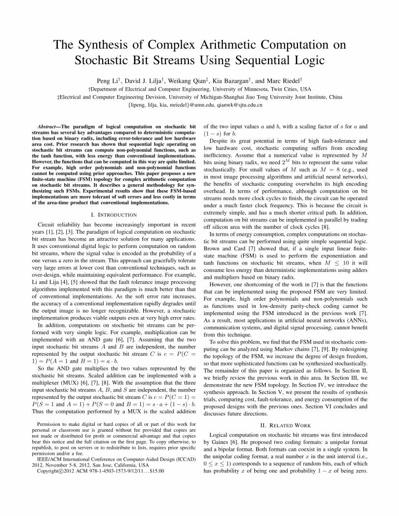
For example, consider an FSM whose output Y is one when thecurrent state is in the set {SN/2, . . . , SN−1} and is zero when thecurrent state is in the set {S0, . . . , SN/2−1}, as shown in the statetransition diagram in Fig. 2. If we let x be the bipolar coding of theinput bit stream X and y be the bipolar coding of the output bit streamY , then the functional relation between x and y is approximately atanh function [7],

y ≈ eN2x − e−

N2x

eN2x + e−

N2x. (1)

Now consider another FSM whose output Y is one when thecurrent state is in the set {S0, . . . , SN−G−1} and is zero when thecurrent state is in the set {SN−G, . . . , SN−1} (where G � N ), asshown in the state transition diagram in Fig. 3. If we let x be thebipolar coding of the input bit stream X and y be the unipolar codingof the output bit stream Y , then the functional relation between xand y is approximately an exponentiation function [7],

y ≈

{e−2Gx, 0 ≤ x ≤ 1,1, −1 ≤ x < 0.

(2)

However, besides these two functions, how to configure otherfunctions based on the linear FSM has not been studied. In 2008, Qianet al. proposed a general approach for synthesizing combinational

logic to implement polynomials on stochastic bit streams [8]. Theprocedure begins by transforming a power-form polynomial into aBernstein polynomial [10]. For example, The polynomial

f(x) =1

4+

9

8x− 15

8x2 +

5

4x3,

can be converted into a Bernstein polynomial of degree 3:

f(x) =2

8B0,3(x) +

5

8B1,3(x) +

3

8B2,3(x) +

6

8B3,3(x),

where each Bi,3(x) (0 ≤ i ≤ 3) is a Bernstein basis polynomial ofthe form

Bi,3(x) =

(3

i

)xi(1− x)3−i. (3)

+

x1x2

xn

MUX

z0

z1

zn

y

Ʃi xi

...

Pr(xi = 1) = x

Pr(zi = 1) = bi

...

Fig. 4. A generalized multiplexing circuit implementing the Bernsteinpolynomial y = B(x) =

∑ni=0 biBi,n(x) with 0 ≤ bi ≤ 1, for

i = 0, 1, . . . , n [8].

A Bernstein polynomial,

y = B(x) =

n∑i=0

biBi,n(x),

with all coefficients bi in the unit interval can be implementedstochastically by a generalized multiplexing circuit, shown in Fig. 4.The circuit consists of an adder block and a multiplexer block. Theinputs to the adder are x1, . . . , xn. The data inputs to the multiplexerare z0, . . . , zn. The outputs of the adder are the selecting inputs tothe multiplexer block.

0,0,0,1,1,0,1,1 (4/8)

0,1,1,1,0,0,1,0 (4/8)

1,1,0,1,1,0,0,0 (4/8)

0,0,0,1,0,1,0,0 (2/8)

x1

x2

x3

1,2,1,3,2,0,2,1

0,1,0,1,0,1,1,1 (5/8)

0,1,1,0,1,0,0,0 (3/8)

1,1,1,0,1,1,0,1 (6/8)

MUX 0,1,0,0,1,1,0,1 (4/8)

z0

z1

z2

z3

y

0

1

2

3

Fig. 5. Logical computation on stochastic bit streams implementing the Bern-stein polynomial f(x) = 2

8B0,3(x) +

58B1,3(x) +

38B2,3(x) +

68B3,3(x)

at x = 0.5. Stochastic bit streams x1, x2 and x3 encode the value x = 0.5.Stochastic bit streams z0, z1, z2 and z3 encode the corresponding Bernsteincoefficients [8].

When the number of ones in the input set {x1, . . . , xn} is i,then the adder will output a binary number equal to i and theoutput y of the multiplexer will be set to zi. The inputs x1, . . . , xn

S0 -----Y=0

SN/2-1 -----Y=0

SN-1 -----Y=1

X=0 X=1

SN/2 -----Y=1

S1 -----Y=0

SN-2 -----Y=1

…… …… ……

…… …… ……

X=1 X=1 X=1 X=1 X=1 X=1 X=1

X=0 X=0 X=0 X=0 X=0 X=0X=0

Fig. 2. The state transition diagram of an FSM implementing a tanh function stochastically. In the figure, the number below each state Si represents theoutput Y of the FSM when the current state is Si (0 ≤ i ≤ N − 1) [7].

S0 -----Y=1

SN-G -----Y=0

SN-1-----Y=0

X=0 X=1

S1 -----Y=1

X=1 …… …… ……

SN-G-1 -----Y=1

…… …… ……

SN-G-2 -----Y=1

X=1 X=1 X=1 X=1 X=1 X=1

X=0 X=0 X=0 X=0 X=0 X=0X=0

Fig. 3. The state transition diagram of an FSM implementing an exponentiation function stochastically. In the figure, the number below each state Sirepresents the output Y of the FSM when the current state is Si (0 ≤ i ≤ N − 1). Note that the number G� N [7].

are independent stochastic bit streams X1, . . . , Xn representing theprobabilities P (Xi = 1) = x ∈ [0, 1], for 1 ≤ i ≤ n. Theinputs z0, . . . , zn are independent stochastic bit streams Z0, . . . , Znrepresenting the probabilities P (Zi = 1) = bi ∈ [0, 1], for0 ≤ i ≤ n, where the bi’s are the Bernstein coefficients. The output ofthe circuit is a stochastic bit stream Y in which the probability of a bitbeing one equals the Bernstein polynomial B(x) =

∑ni=0 biBi,n(x).

A circuit implementation of the above example is shown in Fig. 5 [8].The tanh and the exponentiation functions, as shown in equations

(1) and (2), can also be implemented by this Bernstein polynomial-based approach. However, it requires more hardware than the FSM-based ones. To leverage the low-cost and low-power propertiesof the FSM-based stochastic computation, this paper demonstrateshow to synthesize sophisticated functions based on a new FSMtopology. Based on this technique, more sophisticated functions inANNs, communication systems, and digital signal processing couldbe computed on the stochastic bit streams with lower hardware cost,lower energy consumption, and higher fault-tolerance.

III. THE NEW FSM TOPOLOGY

The state transition diagram of the proposed FSM is shown inFig. 6. It has two inputs (we call them X and K) and in total M ×Nstates, arranged as an M × N two-dimensional array. We normallyset M × N = 2R, where R is a positive integer, because we canimplement an FSM with 2R states by R D flip-flops (DFFs). Inaddition, we set M = 2b

R2 c, and N = 2d

R2 e. The FSM shown

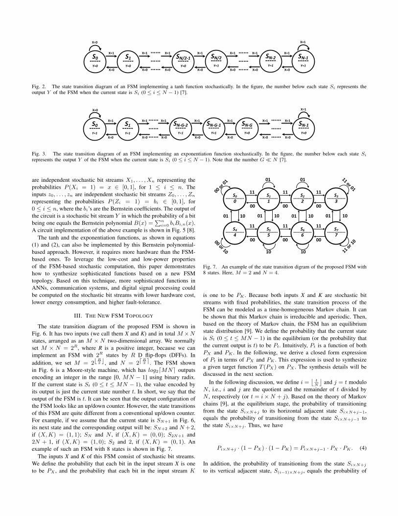
in Fig. 6 is a Moore-style machine, which has log2dMNe outputsencoding an integer in the range [0, MN − 1] using binary radix.If the current state is St (0 ≤ t ≤ MN − 1), the value encoded byits output is just the current state number t. In short, we say that theoutput of the FSM is t. It can be seen that the output configuration ofthe FSM looks like an up/down counter. However, the state transitionsof this FSM are quite different from a conventional up/down counter.For example, if we assume that the current state is SN+1 in Fig. 6,its next state and the corresponding output will be: SN+2 and N+2,if (X,K) = (1, 1); SN and N , if (X,K) = (0, 0); S2N+1 and2N + 1, if (X,K) = (1, 0); S2 and 2, if (X,K) = (0, 1). Anexample of such an FSM with 8 states is shown in Fig. 7.

The inputs X and K of this FSM consist of stochastic bit streams.We define the probability that each bit in the input stream X is oneto be PX , and the probability that each bit in the input stream K

S0 ------------0

S1 ------------1

S2 ------------2

S3 ------------3

S4 ------------4

S5 ------------5

S6 ------------6

S7 ------------7

11

00

11 11

00 00

11

00

11 11

00 00

01 10 01 10 01 10 01 10

00 or 0

111 or 01

11 or 1

000 or 10

01 01

10 10

Fig. 7. An example of the state transition digram of the proposed FSM with8 states. Here, M = 2 and N = 4.

is one to be PK . Because both inputs X and K are stochastic bitstreams with fixed probabilities, the state transition process of theFSM can be modeled as a time-homogeneous Markov chain. It canbe shown that this Markov chain is irreducible and aperiodic. Then,based on the theory of Markov chain, the FSM has an equilibriumstate distribution [9]. We define the probability that the current stateis St (0 ≤ t ≤ MN − 1) in the equilibrium (or the probability thatthe current output is t) to be Pt. Intuitively, Pt is a function of bothPX and PK . In the following, we derive a closed form expressionof Pt in terms of PX and PK . This expression is used to synthesizea given target function T (PX) on PX . The synthesis details will bediscussed in the next section.

In the following discussion, we define i =⌊tN

⌋and j = t modulo

N , i.e., i and j are the quotient and the remainder of t divided byN , respectively (or t = i×N + j). Based on the theory of Markovchains [9], at the equilibrium stage, the probability of transitioningfrom the state Si×N+j to its horizontal adjacent state Si×N+j−1,equals the probability of transitioning from the state Si×N+j−1 tothe state Si×N+j . Thus, we have

Pi×N+j · (1− PX) · (1− PK) = Pi×N+j−1 · PX · PK . (4)

In addition, the probability of transitioning from the state Si×N+j

to its vertical adjacent state, S(i−1)×N+j , equals the probability of

S0 ------------0

…… …… ……

11

00

S1 ------------1

SN-2 ------------N-2

SN-1 ------------N-1

SN ------------N

…… …… ……

SN+1 ------------N+1

S2N-2 ------------2N-2

S2N-1 ------------2N-1

01

……

…

…

……

……

…

…

……

……

…

…

……

……

…

…

……

…… …… ……

S(M-1)N------------(M-1)N

…… …… ……

S(M-1)N+1 ------------(M-1)N+1

SMN-2 ------------MN-2

SMN-1 ------------MN-1

11 11 11

00 00 00

11

00

11 11 11

00 00 00

11

00

11 11 11

00 00 00

10 01 10 01 10 01 10

01 10 01 10 01 10 01 10

01 10 01 10 01 10 01 10

00 or 0

111 or 01

11 or 1

000 or 10 10 10

01 01

00 11

Fig. 6. The FSM has two inputs X and K. The numbers on each arrow represent the transition condition, with the first corresponding to the input X andthe second corresponding to the input K. The FSM has log2dMNe outputs, encoding a value in binary radix. In the figure, the number below each state St(0 ≤ t ≤MN − 1) represents the value encoded by the outputs of the FSM when the current state is St.

transitioning from the state S(i−1)×N+j to the state Si×N+j :

Pi×N+j · (1− PX) · PK = P(i−1)×N+j · PX · (1− PK). (5)

Because all the individual state probabilities Pi×N+j (or Pt) mustsum to unity, we have

MN−1∑t=0

Pt =

M−1∑i=0

N−1∑j=0

Pi×N+j = 1. (6)

Based on equation (4), (5), and (6), we obtain

Pt = Pi×N+j =tix · tjy

M−1∑u=0

N−1∑v=0

tux · tvy, (7)

where tx and ty are,

tx =PX

1− PX· PK

1− PK,

ty =PX

1− PX· 1− PK

PK.

It can be seen that equation (7) is a closed form expression of Ptin terms of PX and PK . In the next section, we discuss how Pt isused to synthesize a given target function.

IV. THE FSM-BASED SYNTHESIS APPROACH

In this section, we introduce how to synthesize a target functionT (PX) based on the proposed FSM. More specifically, we use thecircuit shown in Fig. 8 to synthesize T (PX).

The Proposed

FSM

X

w0 w1

…...

wMN-1

YK

MUXThe current state number

Fig. 8. The circuit for synthesizing target functions.

In Fig. 8, as we introduced in the previous section, the inputs of theproposed FSM are X and K, its output is the current state number,which is connected to the selection inputs of the multiplexer “MUX”,which has M ×N data inputs (w0, w1, · · · , wMN−1). Note that ifthe current state of the FSM is St (0 ≤ t ≤ MN − 1), then thechannel that connects wt to Y will be selected in the “MUX.”

We let X , K, and wt be stochastic bit streams, and define PX tobe the probability of ones in X , PK to be the probability of onesin K, Pwt to be the probability of ones in wt, and PY to be theprobability of ones in Y . Based on the circuit shown in Fig. 8, it canbe seen that the probability that the “MUX” input wt is selected as itsoutput is Pt, because this probability is the same as the probabilitythat the current state of the FSM is St. Thus, we can obtain PY as

PY = P (Y = 1)

=

MN−1∑t=0

P (Y = 1 | wt is selected) · P (wt is selected)

=

MN−1∑t=0

P (wt = 1) · P (wt is selected) =

MN−1∑t=0

Pwt · Pt.

(8)

Note that PY is a function of PX , PK , and Pwt , because Pt is afunction of PX and PK (refer to (7)). It can be seen that equation(8) is a closed form expression of PY . This expression is used tosynthesize the given function T (PX). We define the approximationerror ε as

ε =

∫ 1

0

(T (PX)− PY )2 · d(PX). (9)

The synthesis goal is to compute Pwt and PK to minimize ε. Inthe following, we discuss how to obtain these parameters.

A. How to Compute PwtBy expanding (9), we can rewrite ε as

ε =

∫ 1

0

T (PX)2 · d(PX)− 2

∫ 1

0

T (PX) · PY · d(PX)

+

∫ 1

0

P 2Y · d(PX).

The first term∫ 1

0T (PX)2 · d(PX) is a constant because T (PX) is

given. Thus minimizing ε is equivalent to minimizing the followingobjective function ϕ:

ϕ =

∫ 1

0

P 2Y · d(PX)− 2

∫ 1

0

T (PX) · PY · d(PX). (10)

We define a vector b, a vector c, and a matrix H as follows,

b = [Pw0 , Pw1 , · · · , PwMN−1 ]T ,

c =

−∫ 1

0T (PX) · P0 · d(PX)

−∫ 1

0T (PX) · P1 · d(PX)

...−∫ 1

0T (PX) · PMN−1 · d(PX)

,H = [H0,H1, · · · ,HMN−1]T ,

where Pt (0 ≤ t ≤MN −1) in vector c are defined by equation (7)and Ht (0 ≤ t ≤ MN − 1) in matrix H is a row vector defined asfollows,

Ht =

∫ 1

0Pt · P0 · d(PX)∫ 1

0Pt · P1 · d(PX)

...∫ 1

0Pt · PMN−1 · d(PX)

T

.

Note that (refer to the expression of PY in (8)),

bTHb =

∫ 1

0

P 2Y · d(PX),

cTb = −∫ 1

0

T (PX) · PY · d(PX),

Thus, the objective function ϕ in (10) can be rewrite as

ϕ = bTHb + 2cTb. (11)

We notice that, computing Pwt (i.e., the vector b) to minimizeϕ in the form of equation (11) is a typical constrained quadraticprogramming problem, if PK is a constant. This is because Pt is afunction of both PX and PK (please refer to (7)). When we set PKto a constant, the integral of Pt on PX is also a constant, so arethe vector c and the matrix H. Based on (11), the solution of Pwt(i.e., the vector b) can be obtained using standard techniques [11].Then PK can be solved using a numerical approach, which will bediscussed in the next section.

B. How to Compute PK

As we introduced in the previous section, PK is first set to aconstant. Then we compute Pwt using standard techniques [11] tominimize ε (or the equivalent ϕ). Note that all the values between0 and 1 (with a step 0.001) will be used to set PK in the synthesisprocess. More specifically, we first set PK to 0.001, and compute thecorresponding Pwt and ε. Next, we set PK to 0.002, and computethe corresponding Pwt and ε. So on and so forth. Finally, we set PKto 1, and compute the corresponding Pwt and ε. Among these 1000results of ε, we select the minimum one, and the corresponding PKand Pwt .

C. Summary of the Proposed Synthesis Approach

After we get the optimal values of PK and Pwt , the stochasticbit streams K and wt in Fig. 8 will be generated to implementthe target function T (PX) stochastically. Note that the synthesisapproach discussed in this section also works for other FSM topolo-gies. For example, we can use the same approach to synthesize theexponentiation and tanh functions proposed by Brown and Card [7]based on the FSM topology shown in Fig. 1 [12], [13], [14]. However,that FSM topology cannot be used to synthesize more sophisticatedfunctions, such as high order polynomials and other non-polynomials.We also tried other different FSM topologies in both single inputand two inputs configurations. Only the one proposed in this paperworks. Intuitively, the additional input K and the balanced statetransitions give the proposed FSM more degree of design freedomto synthesize more sophisticated functions.

In the next section, we use three examples to show the synthesiseffect of the proposed approach. Then we compare this work to theprevious ones in terms of hardware cost, energy consumption, andfault-tolerance.

V. EXPERIMENTAL RESULTS

In our experiments, we first present three examples to show thesynthesis results of the proposed approach. Then we compare theproposed approach to the Bernstein polynomial-based approach andthe binary radix representation-based approach in terms of hardwarearea, performance, energy consumption, and fault-tolerance. We usean 8-state FSM (i.e., the one shown in Fig. 7) for all the experiments.

The Proposed FSM (8-State)

X

w0 w1

…...

w7

Y

MUX

K

t0t1t2t3t4...

...

...

01100

00110

t1t2t3t4

0451

t5...

... 0

t1t2t3t4

0111

t5...

... 0

w0w4w5w0w1...

t0

0

t0

0

w0

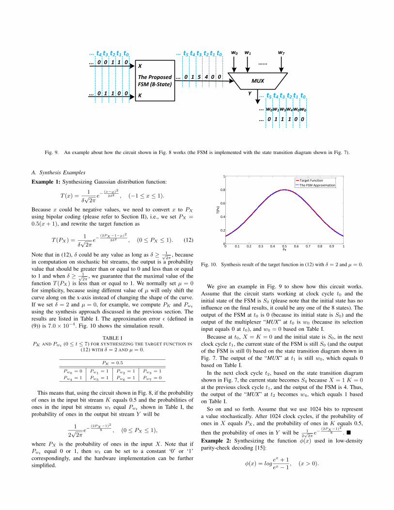
Fig. 9. An example about how the circuit shown in Fig. 8 works (the FSM is implemented with the state transition diagram shown in Fig. 7).

A. Synthesis Examples

Example 1: Synthesizing Gaussian distribution function:

T (x) =1

δ√

2πe− (x−µ)2

2δ2 , (−1 ≤ x ≤ 1).

Because x could be negative values, we need to convert x to PXusing bipolar coding (please refer to Section II), i.e., we set PX =0.5(x+ 1), and rewrite the target function as

T (PX) =1

δ√

2πe− (2PX−1−µ)2

2δ2 , (0 ≤ PX ≤ 1). (12)

Note that in (12), δ could be any value as long as δ ≥ 1√2π

, becausein computation on stochastic bit streams, the output is a probabilityvalue that should be greater than or equal to 0 and less than or equalto 1 and when δ ≥ 1√

2π, we guarantee that the maximal value of the

function T (PX) is less than or equal to 1. We normally set µ = 0for simplicity, because using different value of µ will only shift thecurve along on the x-axis instead of changing the shape of the curve.If we set δ = 2 and µ = 0, for example, we compute PK and Pwtusing the synthesis approach discussed in the previous section. Theresults are listed in Table I. The approximation error ε (defined in(9)) is 7.0× 10−4. Fig. 10 shows the simulation result.

TABLE IPK AND Pwt (0 ≤ t ≤ 7) FOR SYNTHESIZING THE TARGET FUNCTION IN

(12) WITH δ = 2 AND µ = 0.

PK = 0.5

Pw0 = 0 Pw1 = 1 Pw2 = 1 Pw3 = 1

Pw4 = 1 Pw5 = 1 Pw6 = 1 Pw7 = 0

This means that, using the circuit shown in Fig. 8, if the probabilityof ones in the input bit stream K equals 0.5 and the probabilities ofones in the input bit streams wt equal Pwt shown in Table I, theprobability of ones in the output bit stream Y will be

1

2√

2πe−

(2PX−1)2

8 , (0 ≤ PX ≤ 1),

where PX is the probability of ones in the input X . Note that ifPwt equal 0 or 1, then wt can be set to a constant ‘0’ or ‘1’correspondingly, and the hardware implementation can be furthersimplified.

0 0.1 0.2 0.3 0.4 0.5 0.6 0.7 0.8 0.9 10

0.2

0.4

0.6

0.8

1

Px

T(P

x)

Target Function

The FSM Approximation

Fig. 10. Synthesis result of the target function in (12) with δ = 2 and µ = 0.

We give an example in Fig. 9 to show how this circuit works.Assume that the circuit starts working at clock cycle t0 and theinitial state of the FSM is S0 (please note that the initial state has noinfluence on the final results, it could be any one of the 8 states). Theoutput of the FSM at t0 is 0 (because its initial state is S0) and theoutput of the multiplexer “MUX” at t0 is w0 (because its selectioninput equals 0 at t0), and w0 = 0 based on Table I.

Because at t0, X = K = 0 and the initial state is S0, in the nextclock cycle t1, the current state of the FSM is still S0 (and the outputof the FSM is still 0) based on the state transition diagram shown inFig. 7. The output of the “MUX” at t1 is still w0, which equals 0based on Table I.

In the next clock cycle t2, based on the state transition diagramshown in Fig. 7, the current state becomes S4 because X = 1 K = 0at the previous clock cycle t1, and the output of the FSM is 4. Thus,the output of the “MUX” at t2 becomes w4, which equals 1 basedon Table I.

So on and so forth. Assume that we use 1024 bits to representa value stochastically. After 1024 clock cycles, if the probability ofones in X equals PX , and the probability of ones in K equals 0.5,

then the probability of ones in Y will be 1

2√2πe−

(2PX−1)2

8 . �Example 2: Synthesizing the function φ(x) used in low-densityparity-check decoding [15]:

φ(x) = logex + 1

ex − 1, (x > 0).

For this example, we use unipolar coding because we do not dealwith negative values, and set PX = x/α, where α is a scaling factorto map the range of x to unitary. We rewrite the target function interms of PX as

T (PX) = logeαPX + 1

eαPX − 1, (0 < PX ≤ 1). (13)

If we set α = 20, for example, we compute PK and Pwt using theproposed synthesis approach and show the results in Table II. Theapproximation error ε (defined in (9)) is 2.0× 10−4. Fig. 11 showsthe simulation result. �

TABLE IIPK AND Pwt FOR SYNTHESIZING THE TARGET FUNCTION IN (13) WITH

α = 20.

PK = 0.9375

Pw0 = 1 Pw1 = 0 Pw2 = 0 Pw3 = 0

Pw4= 1 Pw5

= 0 Pw6= 0 Pw7

= 0

0 0.1 0.2 0.3 0.4 0.5 0.6 0.7 0.8 0.9 10

0.2

0.4

0.6

0.8

1

Px

T(P

x)

Target Function

The FSM Approximation

Fig. 11. Synthesis result of the target function in (13) with α = 20.

Example 3: Synthesizing the following high order polynomial λ(x)used in low-density parity-check coding [16]:

λ(x) = 0.1575x+ 0.3429x2 + 0.0363x5 + 0.059x6

+ 0.279x8 + 0.1253x9, (0 ≤ x ≤ 1).

For this example, we use unipolar coding because we do not dealwith negative values and x is in the unitary range. We rewrite thetarget function in terms of PX (PX = x) as

T (PX) = 0.1575PX + 0.3429P 2X + 0.0363P 5

X + 0.059P 6X

+ 0.279P 8X + 0.1253P 9

X , (0 ≤ PX ≤ 1).(14)

We compute PK and Pwt using the proposed synthesis approach andshow the results in Table III. The approximation error ε (defined in(9)) is 4.0 × 10−6. Fig. 12 shows the simulation result. Note thatthe bit streams w1 and w5 can be generated with extremely low costusing the technique proposed by Qian et al. [17]. �

TABLE IIIPK AND Pwt FOR SYNTHESIZING THE TARGET FUNCTION IN (14).

PK = 0.1875

Pw0= 0 Pw1

= 0.86 Pw2= 0 Pw3

= 0

Pw4= 0 Pw5

= 0.89 Pw6= 0 Pw7

= 1

0 0.1 0.2 0.3 0.4 0.5 0.6 0.7 0.8 0.9 10

0.2

0.4

0.6

0.8

1

Px

T(P

x)

Target Function

The FSM Approximation

Fig. 12. Synthesis result of the target function in (14).

B. Comparison with the Bernstein Polynomial-Based Approach

As we introduced in Section II, the Bernstein polynomial-basedapproach uses combinational logic (an adder and a multiplexer, asshown in Fig. 5) to perform computation on stochastic bit streams.Hardware area required by this approach depends on the degree ofpolynomial. Table IV lists its area in terms of the number of fan-intwo logic gates [8].

TABLE IVTHE NUMBER OF THE FAN-IN TWO LOGIC GATES FOR COMPUTING

BERNSTEIN POLYNOMIALS OF DEGREE 3, 4, 5, AND 6 [8].

Degree n 3 4 5 6

Number of Gates 22 40 49 58

Note that by using the 8-state FSM shown in Fig. 7, we cansynthesize a polynomial of degree up to 9 (refer to Example 3).In addition, for those non-polynomials, such as the target functionsintroduced in Example 1 and Example 2, the Bernstein polynomial-based approach normally takes at least degree 6 to obtain the samelevel of approximation error. The proposed FSM with 8 states canbe implemented using 3 D-flip-flops (DFFs) as follows,

D2 = XKQ0 +XQ1 +KQ1 +Q1Q0,

D1 = XK̄ +XQ2 + K̄Q2,

D0 = X̄K̄Q1Q̄0 + X̄KQ0 +XKQ1 +XK̄Q0 +XKQ0,

where D0, D1, and D2 are the inputs of the three DFFs, and Q0, Q1,and Q2 are the corresponding outputs. Because it is a Moore FSM,we assign Q2Q1Q0 = 000 for state S0, Q2Q1Q0 = 001 for stateS1, · · · , and Q2Q1Q0 = 111 for state S7. Based on the report ofthe logic synthesis tool Synonsys Design Compiler, the entire circuit(including the multiplexer in Fig. 8) can be implemented using 45fan-in two logic gates. Please note that the evaluation is based ona generalized version of the circuit shown in Fig. 8, if wt is set toa constant ‘0’ or ‘1’, the circuit can be further simplified and thenumber of logic gates can be further reduced. It can be seen that, tosynthesize non-polynomials and polynomials of degree greater than4, the proposed FSM takes less hardware.

In terms of performance, because both techniques compute onstochastic bit streams, they have equivalent processing time. In termsof energy consumption, we assume that given a CMOS technology,a digital circuit consumes a constant power dissipation per unitarea. We use the product of area and processing time as a metricof the energy consumption [7]. Because these two techniques have

equivalent processing time, the FSM-based approach consumes lessenergy when computing non-polynomials and high order polynomialswith degree larger than 4.

In terms of fault-tolerance, we compare the two techniques whenthe input data is corrupted with noise. We evaluate the fault-tolerantperformance on circuits implementing the target functions intro-duced in the last section and other functions such as trigonometricfunctions (sin(x), cos(x), and tan(x)) and logarithmic functions(y = log2(x), y = log10(x), and y = ln(x)). The length of thestochastic bit streams which are used to represent a value is set to1024. We define the error ratio γ as the percentage of random bitflips that occur in the computation. We choose the error ratio γ to be0%, 0.5%, 1%, 5%, and 10%. For example, under 10% error ratio,102 of 1024 bits will be flipped in the computation. To measure theimpact of the noise, we evaluated each target function at 13 distinctinput data points: 0.2, 0.25, 0.3, · · · , 0.8. For each error ratio γ,each target function, and each evaluation point, we simulated boththe FSM-based implementation and the Bernstein polynomial-basedimplementation 1000 times. We averaged the relative errors over allsimulations. Finally, for each error ratio γ, we averaged the relativeerrors over all target functions and all evaluation points. Table Vshows the average relative error of the two different implementationsversus different γ values. It can be seen that these two techniqueshas almost equivalent fault-tolernace (the difference is less than0.5%), because both techniques perform computation on stochasticbit streams.

TABLE VRELATIVE ERROR FOR THE FSM-BASED IMPLEMENTATION AND THE

BERNSTEIN POLYNOMIAL-BASED IMPLEMENTATION OF TARGETFUNCTION COMPUTATION VERSUS THE ERROR RATIO γ IN THE INPUT

DATA.

Error Ratio γ (%) 0 0.5 1 5 10Relative Error of the FSM (%) 2.26 2.78 3.16 6.75 11.2Relative Error of Bernstein (%) 2.21 2.72 3.36 6.25 11.7

C. Comparison with the Binary Radix-Based Approach

Assume that M is the number of bits used to represent a numericalvalue in binary radix. In order to get the same resolution for computa-tion on stochastic bit streams, we need a 2M -bit stream to representthe same value. Both Qian et al. [8] and Brown et al. [7] showedthat, when M ≤ 10, computation on stochastic bit streams hasbetter performance than the ones based on binary radix using addersand multipliers in terms of hardware area and energy consumption.In fact, in most applications of the stochastic computation, M isbetween 8 to 10 [7], [8]. As we discussed in the Section V-B, theproposed approach using FSM has better performance than the oneproposed by Qian et al. [8] for computing non-polynomials and highorder polynomials. Thus, when M ≤ 10, the proposed approachalso has better performance than the ones using binary radix forthose functions. In addition, computing on stochastic bit streamsoffers tunable precision: as the length of the stochastic bit streamincreases, the precision of the value represented by it also increases.Thus, without hardware redesign, we have the flexibility to trade-offprecision and computation time. The main issue of this computingtechnique is the long latency. However, it can be solved by using afaster clock frequency, because its logic is simple and has shortercritical path. Parallel computing can also be used to solve this issue.For example, in digital image processing applications, we can processmultiple pixels in an image in parallel. In ANN applications, we canprocess the computation on multiple neurons in parallel.

VI. CONCLUSION

This paper proposed a new FSM topology to synthesize compu-tation on stochastic bit streams for complex and useful functions.Compared to other implementations, the resulting circuits are lesscostly in terms of hardware area and energy consumption. In futurework, we will study synthesis techniques for general purpose compu-tation using these techniques. Our eventual goal is a fully stochasticdesign of a microprocessor.

ACKNOWLEDGMENT

This work was supported in part by National Science Foundationgrant no. CCF-1241987. Any opinions, findings and conclusions orrecommendations expressed in this material are those of the authorsand do not necessarily reflect the views of the NSF. This work is alsosupported in part by the Minnesota Supercomputing Institute and bya donation from NVIDIA.

REFERENCES

[1] N. Iqbal, M. Siddique, and J. Henkel, “Seal: soft error aware low powerscheduling by monte carlo state space under the influence of stochasticspatial and temporal dependencies,” in Design Automation Conference(DAC), 2011 48th ACM/EDAC/IEEE, pp. 134–139, IEEE, 2011.

[2] X. Shih, H. Lee, K. Ho, and Y. Chang, “High variation-tolerant obstacle-avoiding clock mesh synthesis with symmetrical driving trees,” inProceedings of the International Conference on Computer-Aided Design,pp. 452–457, IEEE Press, 2010.

[3] S. Rehman, M. Shafique, F. Kriebel, and J. Henkel, “Reliable softwarefor unreliable hardware: embedded code generation aiming at reliability,”in Proceedings of the seventh IEEE/ACM/IFIP international conferenceon Hardware/software codesign and system synthesis, pp. 237–246,ACM, 2011.

[4] P. Li and D. J. Lilja, “A low power fault-tolerance architecture for thekernel density estimation based image segmentation algorithm,” in IEEEInternational Conference on Application - specific Systems, Architecturesand Processors, ASAP’11, 2011.

[5] P. Li and D. J. Lilja, “Using stochastic computing to implement digitalimage processing algorithms,” in IEEE International Conference onComputer Design, ICCD’11, 2011.

[6] B. Gaines, “Stochastic computing systems,” Advances in InformationSystems Science, vol. 2, no. 2, pp. 37–172, 1969.

[7] B. D. Brown and H. C. Card, “Stochastic neural computation I: Compu-tational elements,” IEEE Transactions on Computers, vol. 50, pp. 891–905, September 2001.

[8] W. Qian and M. D. Riedel, “The synthesis of robust polynomialarithmetic with stochastic logic,” in 45th ACM/IEEE Design AutomationConference, DAC’08, pp. 648–653, 2008.

[9] A. A. Markov, “Extension of the limit theorems of probability theory toa sum of variables connected in a chain,” reprinted in Appendix B of:R. Howard. Dynamic Probabilistic Systems, volume 1: Markov Chains.John Wiley and Sons, 1971.

[10] G. Lorentz, Bernstein Polynomials. University of Toronto Press, 1953.[11] G. Golub and C. Van Loan, Matrix computations, vol. 3. Johns Hopkins

Univ Pr, 1996.[12] P. Li, W. Qian, M. Riedel, K. Bazargan, and D. Lilja, “The synthesis of

linear finite state machine-based stochastic computational elements,” inDesign Automation Conference (ASP-DAC), 2012 17th Asia and SouthPacific, pp. 757–762, IEEE, 2012.

[13] P. Li, D. J. Lilja, W. Qian, and K. Bazargan, “Using a two-dimensionalfinite-state machine for stochastic computation,” in International Work-shop on Logic and Synthesis, IWLS’12, 2012.

[14] P. Li, W. Qian, and D. J. Lilja, “A stochastic reconfigurable architecturefor fault-tolerant computation with sequential logic,” in IEEE Interna-tional Conference on Computer Design, ICCD’12, 2012.

[15] W. Ryan, “An introduction to ldpc codess,” 2003.[16] T. Richardson, M. Shokrollahi, and R. Urbanke, “Design of capacity-

approaching irregular low-density parity-check codes,” Information The-ory, IEEE Transactions on, vol. 47, no. 2, pp. 619–637, 2001.

[17] W. Qian, M. Riedel, K. Bazargan, and D. Lilja, “The synthesis ofcombinational logic to generate probabilities,” in Proceedings of the2009 International Conference on Computer-Aided Design, pp. 367–374, ACM, 2009.