The Structure of the FV3 Solver

Lucas Harris

and the GFDL FV3 Team

FV3 Summer School

12 June 2018

FV3 Design Philosophy

• Discretization should be guided by physical principles as much as possible• Finite-volume, integrated form of conservation laws

• Upstream-biased fluxes

• Operators “reverse engineered” to achieve desired properties

• Computational efficiency is crucial. Fast models can be good models!

• Solver should be built with vectorization and parallelism in mind

• Dynamics isn’t the whole story! Coupling to physics and the ocean is important.

Finite-volume methodology

• In FV3, all variables are 3D cell- or face-means…not gridpoint values

• We solve not the differential Euler equations but their cell-integrated forms using integral theorems• Everything is a flux, including the momentum equation

• Mass conservation is ensured, to rounding error

• C-D grid: Vorticity computed exactly; accurate divergence computation

• Mimetic: Physical properties recovered by discretization, particularly Newton’s 3rd law

• Fully compressible: calculation is horizontally local

Outline of the FV3 solver

Abstract of FV3

• Gnomonic cubed-sphere grid for scalability and uniformity

• Fully-compressible vector-invariant Euler equations

• Vertically-Lagrangian dynamics

• Hybrid-pressure terrain-following coordinate (but others exist)

• C-D grid discretization

• Forward-in-time 2D Lin-Rood advection using PPM operators

• Fully nonhydrostatic with semi-implicit solver• Runtime hydrostatic switch

FV3 time integration sequence

• FV3 is a forward-in-time solver• Flux-divergence terms and physics tendencies evaluated forward-in-time

• Pressure-gradient and sound-wave terms evaluated backward-in-time for stability

• Lagrangian vertical coordinate: flow constrained along time-evolving Lagrangian surfaces. This greatly simplifies the inner “acoustic” or “Lagrangian dynamics” timestep.

fv_dynamics()FV3 solver

dyn_core()Lagrangian dynamics

fv_tracer2d()Sub-cycled tracer transport

OpenMP on k

Lagrangian_to_Eulerian()Vertical Remapping(i,k) OpenMP on j

c_sw(), etc.C-grid solver

d_sw()Forward Lagrangian dyn.

OpenMP on k

update_dz_d()Forward δz evaluation

OpenMP on k

one_grad_p()/nh_p_grad()Backwards horizontal PGF

OpenMP on k

riem_solver()Backwards vertical PGF, sound wave processes

(i,k) OpenMP on j

[physics]

fv_update_phys()Consistent field update

fv_dynamics()FV3 solver

dyn_core()Lagrangian dynamics

fv_tracer2d()Sub-cycled tracer transport

OpenMP on k

Lagrangian_to_Eulerian()Vertical Remapping(i,k) OpenMP on j

c_sw(), etc.C-grid solver

d_sw()Forward Lagrangian dyn.

OpenMP on k

update_dz_d()Forward δz evaluation

OpenMP on k

one_grad_p()/nh_p_grad()Backwards horizontal PGF

OpenMP on k

riem_solver()Backwards vertical PGF, sound wave processes

(i,k) OpenMP on j

[physics]

fv_update_phys()Consistent field update

dt_atmosk_split

“remapping” loop

n_split“acoustic” loop

FV3 time integration sequence

• The innermost acoustic timestep advances all processes (except vertical sound-wave modes) explicitly. During these timesteps the Lagrangian surfaces are allowed to deform freely.

• Tracers are sub-cycled since their stability condition is much less restrictive than the sound- or gravity-wave modes. Tracer advection is done using the air mass fluxes accumulated during the acoustic timesteps, for consistency.

• After the vertical remapping back to the Eulerian vertical levels, the state can be handed off to the physics.

Time integration: Namelist Options

• dt_atmos (in atmos_model_nml): Timestep for the entire FV3 solver; also equal to the physics timestep, in seconds.

• k_split: Number of vertical remappings per long timestep. Vertical remapping timestep is equal to dt_atmos / k_split .

• n_split: Number of acoustic timesteps per vertical remapping timestep. The acoustic timestep is equal to dt_atmos / (k_split x n_split)

• hydrostatic: whether to use the (much faster) hydrostatic solver. This does not require a re-compile (but some #ifdefs are more appropriate for the hydrostatic dynamics)

Recommended Timestepping Values

Recommended first-guess values.

In some cases additional k_splits(reducing n_split so acoustic timestep is constant) can be more stable, with the added cost of additional vertical remappings.

Regional domains with lower tops (and so not seeing the polar night jets) may be able to take longer timesteps.

Average Grid-width (km)

dt_atmos k_split n_split acoustic dt

c48 200 3600 2 6 300

c96 100 1800 2 6 150

c192 50 900 2 6 75

c384 25 450 2 6 37.5

c768 13 225 2 6 18.75

c1152 9 150 2 6 12.5

c3072 3 90 2 10 4.5

The Cubed-Sphere GridThe 3 in FV3

The Cubed-Sphere Grid

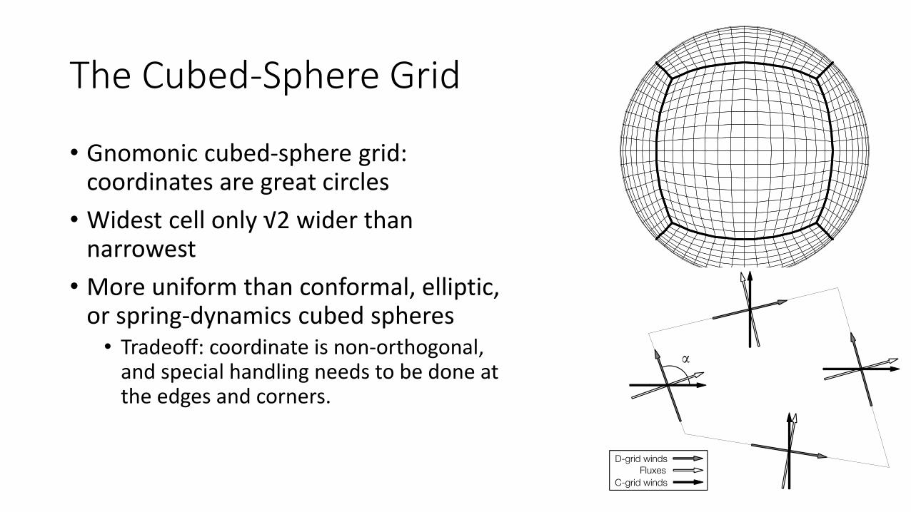
• Gnomonic cubed-sphere grid: coordinates are great circles

• Widest cell only √2 wider than narrowest

• More uniform than conformal, elliptic, or spring-dynamics cubed spheres• Tradeoff: coordinate is non-orthogonal,

and special handling needs to be done at the edges and corners.

The Cubed-Sphere Grid

• Gnomonic cubed-sphere is non-orthogonal

• Instead of using numerous metric terms, use covariant and contravariant winds• Solution winds are covariant, advection is by

contravariant winds

• KE is half the product of the two

• Winds u and v are defined in the local coordinate: rotation needed to get zonal and meridional components

Cubed-Sphere Grid: Namelist Options

• npx, npy: Number of grid corners in each direction. A global cubed sphere must use the same in both directions; nested, regional, or doubly-periodic domains do not.

• ntiles: Number of tiles on a domain. For the cubed sphere this must be 6; currently the nest is restricted to 1.

• layout: 2-element array for the number of MPI domain decompositions in each direction on each tile. These values should be divisors of (npx - 1) and (npy - 1)• Total number of cores is layout(1) x layout(2) x 6.

Lagrangian Dynamics in FV3What they are

What the equations are

How they are solved

What are Lagrangian Dynamics?

• The Euler equations can be written in Lagrangian or Eulerian forms…or Eulerian in the horizontal, and Lagrangian in the vertical

• This constrains the flow along quasi-horizontal surfaces

• Surfaces deform during the integration, representing vertical motion and advection “for free”

• Requires layer thickness to be a prognostic variable

Prognostic Variables

δp Total air mass (including vapor and condensates)Equal to hydrostatic pressure depth of layer

θv Virtual potential temperature

u, v Horizontal D-grid winds in local coordinate(defined on cell faces)

w Vertical winds

δz Geometric layer depth

qi Passive tracers

Cell-mean pressure, density, divergence, and specific heat are all diagnostic quantitiesAll variables are layer-means in the vertical: No vertical staggering

Lagrangian Dynamics:Flux-form advection

• Advection is not just for passive tracers! Nearly everything in FV3 is a flux• Even the KE gradient terms can be expressed as scalar fluxes

• Built from 1D PPM operators through the Lin-Rood FV scheme

• Again: advection is along Lagrangian surfaces

Piecewise-Parabolic Method:The cornerstone of finite-volume numerics

• Collela & Woodward (1984) extension to higher order of the Van Leer (1979) piecewise-linear method, itself an extension of Godunov’s first-order finite-volume scheme

• The internal variation of each grid cell is approximated by a parabola, from which the fluxes through each cell interface can be integrated

Piecewise-Parabolic Method:The cornerstone of finite-volume numerics• The parabola’s profile can be chosen to

fit the data the most closely, to get the highest-order (formally 4th if ∆x is constant) solution. But you are free to do much more.

• The parabolas can be flattened (or steepened) based on the adjacent grid cells. This is useful for shape-preservation (monotonicity, positive-definite) or for simply eliminating undesirable 2∆x noise

“Imagine PPM as something akin to the Toll House chocolate chip cookie recipe. The cookies you get by following the package exactly are really, really good. At the same time, you can modify the recipe to produce something even better while staying true to the basic framework. The basic cookies will get you far, but with some modification you might just win contests or simply impress your friends. PPM is just like that.”

wjrider.wordpress.com/2017/11/17/the-piecewise-parabolic-method-ppm/

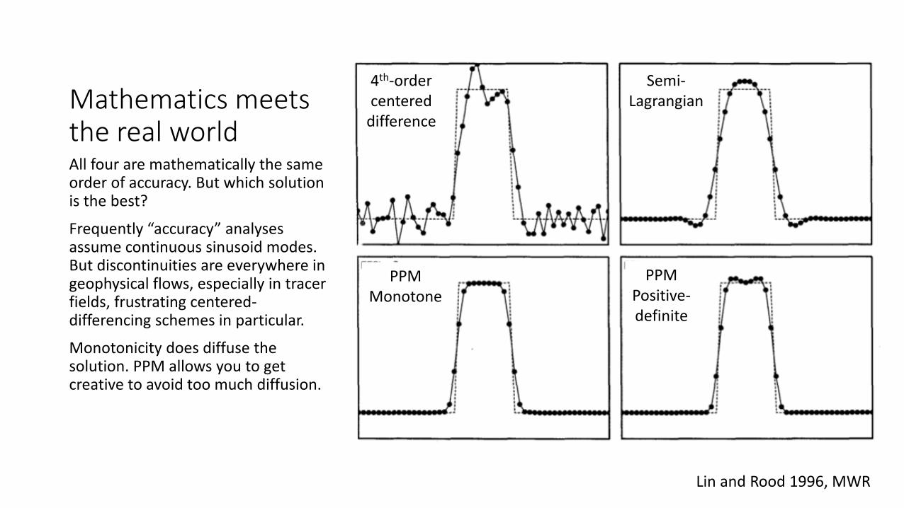
Mathematics meets the real worldAll four are mathematically the same order of accuracy. But which solution is the best?

Frequently “accuracy” analyses assume continuous sinusoid modes. But discontinuities are everywhere in geophysical flows, especially in tracer fields, frustrating centered-differencing schemes in particular.

Monotonicity does diffuse the solution. PPM allows you to get creative to avoid too much diffusion.

Lin and Rood 1996, MWR

4th-ordercentered

difference

Semi-Lagrangian

PPMMonotone

PPMPositive-definite

Lin-Rood FV Advection

• F, G are flux-form conservative PPM operators; f, g are advective form PPM operators.

• This reverse-engineered form cancels the leading-order deformation error while ensuring mass conservation, and so the Courant number restriction is independent in both directions• max(Cx,Cy) ≤ 1 instead of Cx + Cy ≤ 1

Lagrangian Dynamics:Tracer advection and sub-cycling• Tracers can be advected with a longer timestep than the dynamics

• FV3 permits accumulation of mass fluxes during Lagrangian dynamics.These fluxes are then used to compute the advection of tracers before the vertical remapping• Typically one or two tracer timesteps is sufficient for stability. The number is

determined dynamically from the domain-maximum wind speed

• Tracer advection is always monotone or positive definite to avoid new extrema. Explicit diffusion is not used.

Lagrangian Dynamics:C-D grid solver• FV3 solves for the (purely horizontal)

D-grid staggered winds. But solver requires face-normal and time-mean fluxes

• To compute time step-mean fluxes, the C-grid winds are interpolated and then advanced a half-timestep.• A sort of simplified Riemann solver

• The C-grid solver is the same as the D-grid, but uses lower-order fluxes for efficiency

• Two-grid discretization and time-centered fluxes avoid computational modes

Lagrangian Dynamics:Momentum equation• FV3 solves the flux-form vector invariant

equations

• Nonlinear vorticity flux term in momentum equation, confounding linear analyses

• D-grid allows exact computation of absolute vorticity—no averaging!

• Vorticity uses same flux as δp: consistency improves geostrophic balance, and SW-PV advected as a scalar!

Lagrangian Dynamics:Momentum equation• FV3 solves the flux-form vector invariant

equations

• Nonlinear vorticity flux term in momentum equation, confounding linear analyses

• D-grid allows exact computation of absolute vorticity—no averaging!

• Vorticity uses same flux as w: consistency improves nonlinear balance, and updraft helicity advected as a scalar!

Many flows are vorticalNot just large-scale flows

NASA Goddard

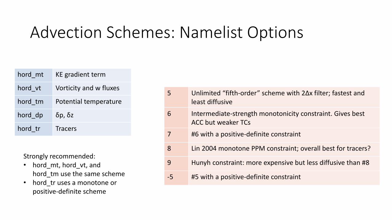
Advection Schemes: Namelist Options

hord_mt KE gradient term

hord_vt Vorticity and w fluxes

hord_tm Potential temperature

hord_dp δp, δz

hord_tr Tracers

Strongly recommended:• hord_mt, hord_vt, and

hord_tm use the same scheme• hord_tr uses a monotone or

positive-definite scheme

5 Unlimited “fifth-order” scheme with 2∆x filter; fastest and least diffusive

6 Intermediate-strength monotonicity constraint. Gives best ACC but weaker TCs

7 #6 with a positive-definite constraint

8 Lin 2004 monotone PPM constraint; overall best for tracers?

9 Hunyh constraint: more expensive but less diffusive than #8

-5 #5 with a positive-definite constraint

Backward horizontalpressure gradient force• Computed from Newton’s second and third

laws, and Green’s Theorem

• Errors lower, with much less noise, compared to traditional evaluations• Purely horizontal

no along-coordinate projection• PGF equal and opposite—3rd law!

Momentum conserved• Curl-free in the absence of density gradients

• Nonhydrostatic and hydrostatic components can be computed separately• log(phyd) PGF more accurate

Backward horizontalpressure gradient force• Computed from Newton’s second and third

laws, and Green’s Theorem

• Errors lower, with much less noise, compared to traditional evaluations• Purely horizontal

no along-coordinate projection• PGF equal and opposite—3rd law!

Momentum conserved• Curl-free in the absence of density gradients

• Nonhydrostatic and hydrostatic components can be computed separately• log(phyd) PGF more accurate

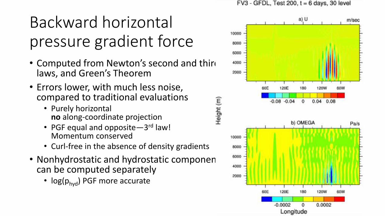
Backward horizontalpressure gradient force• Computed from Newton’s second and third

laws, and Green’s Theorem

• Errors lower, with much less noise, compared to traditional evaluations• Purely horizontal

no along-coordinate projection• PGF equal and opposite—3rd law!

Momentum conserved• Curl-free in the absence of density gradients

• Nonhydrostatic and hydrostatic components can be computed separately• log(phyd) PGF more accurate

Dynamics namelist options

• npz: number of vertical levels, chosen from a list of pre-defined settings in fv_eta.F90 . Many of these are very carefully constructed to avoid instability and place the highest resolution where it is needed.

• fill: whether to perform a simple vertical-borrowing filling on tracers to eliminate the tiny negatives that may crop up

Dynamics namelist options

• dnats: number of tracers to not advect. This will skip the last dnatstracers in the field_table file. Typically cloud fraction is not advected, for example

• z_tracer: option to dynamically compute sub-cycled tracer timestepping on each level individually. This can greatly improve efficiency since upper-level winds are much stronger and have a more strict Courant number restriction

A few debugging and diagnostic options

• print_freq: frequency (in hours if > 0; in timesteps if < 0) of diagnostic outputs; max/min/ave, global integrals, etc.

• range_warn: whether to check the ranges of values at different places in the core, and print out location of bad values

• fv_debug: print great quantities of solver information

• no_dycore: turn OFF the dynamics, enabling the column physics mode; good for debugging or testing “single column”.

Diffusion mechanisms and upper boundary conditions

•MYTH: Numerical diffusion is evil, only used to cover for discretization deficiencies, and should be avoided at all costs.

•TRUTH: Numerical diffusion is a necessary part of any model used for environmental simulation.

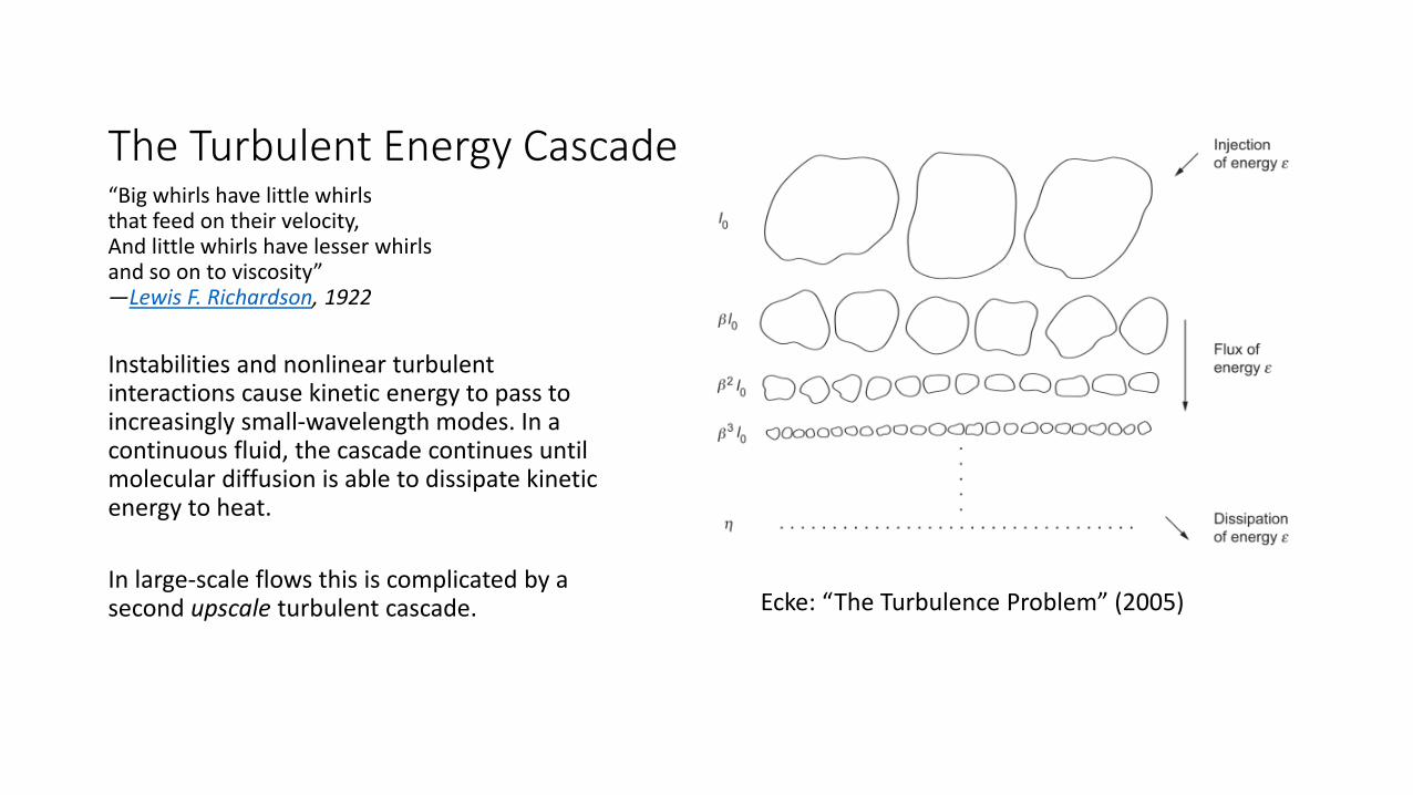
The Turbulent Energy Cascade“Big whirls have little whirlsthat feed on their velocity,And little whirls have lesser whirlsand so on to viscosity”—Lewis F. Richardson, 1922

Instabilities and nonlinear turbulent interactions cause kinetic energy to pass to increasingly small-wavelength modes. In a continuous fluid, the cascade continues until molecular diffusion is able to dissipate kinetic energy to heat.

In large-scale flows this is complicated by a second upscale turbulent cascade. Ecke: “The Turbulence Problem” (2005)

The Turbulent Energy Cascade

Dissipative scales ( < 10-2 m) are never resolved in environmental simulation. Without artificial diffusion, energy would accumulate at grid scales until the model crashes. Numerical diffusion represents the need of the model to represent an unresolved physical process. Since this occurs horizontally it needs to be part of the dynamical core—it cannot be represented in column physics.Artificial diffusion is necessary—whether explicit or not.

• Implicit diffusion: damping time-integration schemes, monotonicity constraints, Lagrangian remapping

• Explicit diffusion: Smagorinsky/Lilly diffusion, hyperdiffusion, divergence damping

Numerical diffusion

• Numerical noise can also arise in realistic simulation from bad initial/boundary data, strange physics interactions, and miscellaneous model pathologies.

• Properly configured numerical diffusion is a powerful tool to improvea simulation, especially for applications where a particular phenomenon is studied (Zhao, Held and Lin 2012; Tompkins and Semie 2017; Pressel et al 2017). In particular S2S and climate simulations may benefit from added diffusion.

• FV3’s diffusion is highly configurable, to represent the very broad range of applications for which it is used.

Implicit and Flux damping

• The physically-consistent design of FV3 (FV PGF, upwind numerics, cancellation of splitting error) produces very few computational modes.

• Monotone fluxes are sufficient to eliminate noise in the rotational modes. This is “smart” and very selective diffusion, but may be too strong for mesoscale (< 50 km) resolutions, especially when nonhydrostatic effects become important

Flux Damping

• If non-monotone methods are used, then flux (or “vorticity”) damping can be applied. This adds diffusion to the fluxes—so conservation is not affected, even for higher-order damping.

• Flux damping is only applied to the fluxes of vorticity and to scalars advected on the acoustic timestep (δp, δz, θv, w, etc.), to maintain dynamical consistency. It is not applied to sub-cycled tracers.

• The kinetic energy lost to flux damping can be restored, in part or in whole, as heat—improving energy conservation.

Divergence damping

• The C-D grid design allows divergent modes to escape even the implicit diffusion in FV3. So the cascade proceeds to grid scale unimpeded. No direct implicit diffusion to divergence.

• To represent the physical process of dissipation, we add scale-selective explicit divergence damping. This allows divergent and rotational modes to be damped separately, because the solver treats divergence and vorticity separately.

• Note that all implicit (except vertical remapping) and explicit diffusion is along Lagrangian surfaces.

Numerical Damping: Namelists

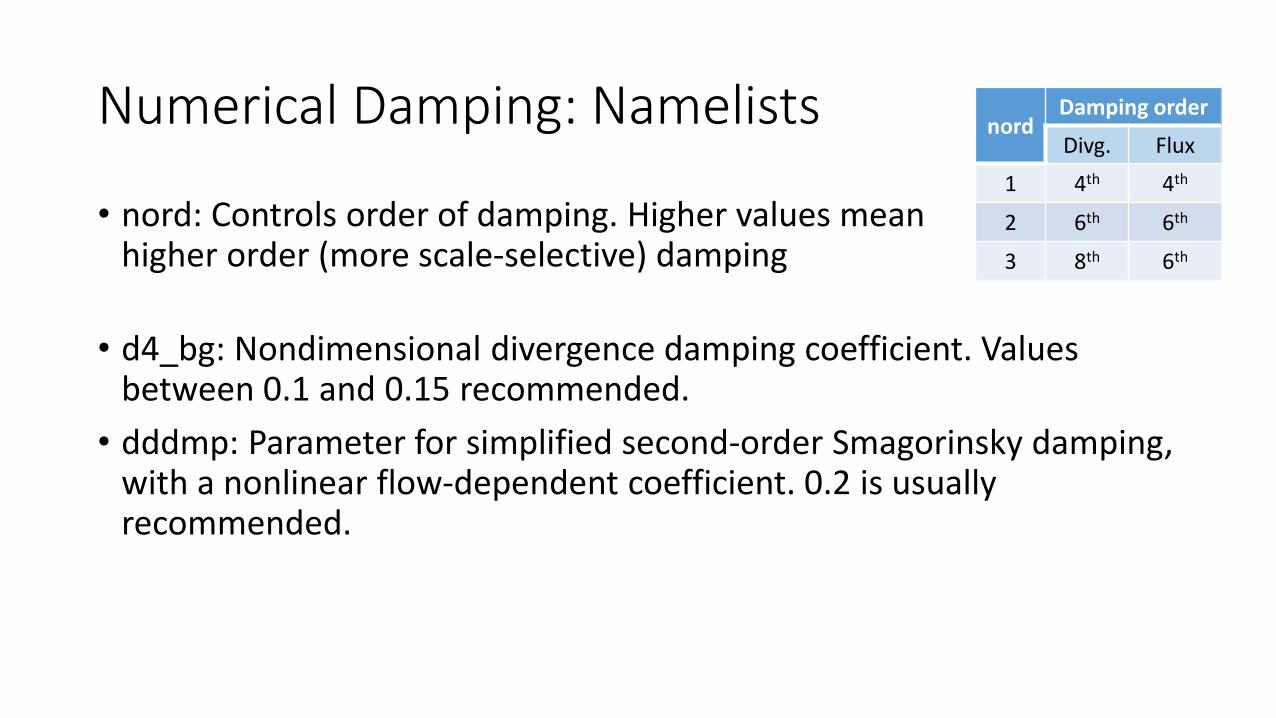
• nord: Controls order of damping. Higher values mean higher order (more scale-selective) damping

• d4_bg: Nondimensional divergence damping coefficient. Values between 0.1 and 0.15 recommended.

• dddmp: Parameter for simplified second-order Smagorinsky damping, with a nonlinear flow-dependent coefficient. 0.2 is usually recommended.

nordDamping order

Divg. Flux

1 4th 4th

2 6th 6th

3 8th 6th

Numerical Damping: Namelist Items

• do_vort_damp: Logical flag for enabling flux (“vorticity”) damping.

• vtdm4: Nondimensional coefficient for flux damping. This can be much smaller than d4_bg; values between 0.02 and 0.06 are recommended.

• d_con: Fraction of damped kinetic energy from flux damping restored as heat. Set to 0.0 to disable this conversion; 1.0 restores all energy.

• delt_max: Limit on heating from damped kinetic energy (K/s). This is useful to improve stability since damping can get large in some regions of strong deformation. Values between 0.002 and 0.008 are recommended.

The Upper Boundary

• FV3 has a flexible upper boundary (constant pressure) which greatly reduces the reflection of vertically-propagating gravity waves, compared to the rigid lid (constant height) of many models. So the sponge layer can be much shallower.

• Gravity waves can grow very large without breaking near the model top (0.6 mb in current GFS): the density gets very low so amplitude must increase to maintain constant momentum flux. These waves should be removed near model top.

• Stratospheric circulation can also be “tuned” through the proper use of upper boundary damping

The Sponge Layer

• In FV3 the top two layers are reserved as sponge layers. These layers are usually very deep (∆z) so some dissipation of vertically-propagating waves has already been accomplished.

• In these layers a much stronger, less scale-selective second-order damping (divergence and flux) is applied on the acoustic timestep.

Rayleigh Damping

• A drag force applied to all three wind components with a specified timescale.

• Lost kinetic energy is converted to heat on global domains (not on nest or regional).

• The timescale is dependent on pressure; shortest (strongest) at the top layer, and increasingly weak lower down until rf_cutoff is reached.

2∆z Shear Instability Filter

• Energy-, momentum-, and mass-conserving subgrid local vertical mixing whenever Ri < 1; amount of mixing is proportional to 1-Ri (total if Ri ≤ 0) and acts on a given timescale.

• Very useful for handling breaking large-amplitude waves in the middle atmosphere. Only applied in the top n_sponge number of layers.

Upper Boundary: Namelist Options

• d2_bg_k1: Strength of second-order damping in top layer (k=1). Values between 0.15 and 0.2 recommended.

• d2_bg_k2: …in second layer (k=2). Recommend values between 0.02 and 0.1.

• tau: Timescale (days, smaller is stronger) of Rayleigh damping. Recommend 5 for 13-km, 3 or 1.5 for 3-km.

• rf_cutoff: Level (in Pa) below which no Rayleigh damping is applied. Recommend values between 5.e2 and 50.e2 (higher values for regional domains).

Upper Boundary: Namelist Options

• n_sponge (misleading artifact name): Number of layers from the top on which 2∆z filter is applied. Recommend applying to layers above 100 mb.

• fv_sg_adj: Timescale (s, smaller is stronger) of 2∆z filter. Use values larger than dt_atmos to avoid interfering with vertical diffusion modules in the physics.

Vertical processes:Vertical elastic termsand Lagrangian vertical coordinate

The Lagrangian Vertical Coordinate

• The domain is separated into a number of quasi-horizontal Lagrangian layers (k index, k=1 at top)

• All flow is within the layers (“logically” horizontal)

• No cross-layer layer flow or diffusionVertical motion deforms the layers instead

• The mass δp and height δz are prognostic variables. Height and pressure of each layer are dynamically computed.

The Lagrangian Vertical Coordinate

• Lagrangian coordinate works for any base coordinate• Hybrid-pressure, hybrid-height, and hybrid-isentropic coordinates

have been successfully used

• Vertical advection is implicit through the vertical movement of layers • There is no Courant number restriction or time-splitting!

• Vertical advection does not need a separate computation. Computing δp and δz is sufficient.

• Implicit advection not only saves time but also permits very thin layers without requiring a smaller timestep

Vertical Remapping

• Periodically, a highly-accurate conservative remapping is done to avoid layers becoming infinitismally thin (δp → 0)• Remapping interval like Lagrangian advection’s timestep:

longer timesteps yield less overall artificial diffusion

• This is the only way cross-layer diffusion is introduced!!

• Remapping is done conservatively by integrating a highly accurate reconstruction: either PPM or a (more accurate) cubic spline, with appropriate limiters

• Remapping is from deformed layers back to the “Eulerian” reference coordinate

• Interface pressures defined pk = ak + bk * ps

Vertical Remapping: Namelist Options • kord_mt, kord_wz, kord_tr: Vertical

remapping scheme for momentum, vertical velocity, and tracers, respectively. There are a wide variety of schemes; table lists recommended options.

• kord_tm: Vertical remapping scheme for temperature (if < 0) or potential temperature (if > 0). Recommend a negative value.

kord

4 Monotone PPM

6 Vanilla PPM

7 PPM with Hyunh’s monotonicity constraint (more expensive but less diffusive)

9 Monotonic Cubic Spline

10 Selectively (local extrema retained) monotonic Cubic Spline with 2∆z oscillations removed

11 Non-monotonic cubic spline with 2∆z oscillations removed

The Energy Fixer

• Earlier versions of FV remapped on total energy and re-derived temperature, which was properly energy conserving. But this could be noisy and inaccurate due to the exponential increase in PE near model top.

• Recent versions can remap either potential temperature or temperature. The latter does not suffer from an exponential increase at high altitudes. However remapping is not energy conservative.

• Lost energy can be restored globally through an energy fixer. The fixer adds the lost energy to the temperature in a way to ensure pressure gradients are not altered (and so no spurious PGF created).

The Energy Fixer: Namelist Option

• consv_te: Fraction of lost energy globally restored as heat. Ideally this would be set to 1, but often the physics does not correctly conserve energy and so this value should be tuned. In AM2 and HiRAM 0.7 was used; in AM4 0.6 is used.

Semi-implicit solver

• Vertical pressure gradient and non-advective changes to layer depth δz are solved by semi-implicit solver• Vertically-propagating sound waves weakly damped

• This is all that is needed to make the classic FV hydrostatic algorithm nonhydrostatic• Fully compressible and nonhydrostatic! Full Euler equations solved

• w, δz advected as other variables—consistent!

• Nonhydrostatic horizontal PGF evaluated same way as hydrostatic

A little bit about initialization

FV3 has a host of online and offline utilities to generate grids, orography, and initial conditions from cold start

• Any grid can be generated in seconds• Initialize from NCEP or EC analyses• Remap from different vertical spacings• Comprehensive topography generation, including subgrid orography• Advanced FCT orography filter allows preservation of total topography, peaks,

and valleys; limits slope steepness; and prevents nonzero topography in the ocean

• There is an extensive nudging module in FV3; a full explanation would lie beyond the scope of this presentation

Initialization: Namelist Options

• external_ic: enable module for reading ICs from external file

• nggps_ic: Read regridded GFS ICs. Does no horizontal interpolation.

• ncep_ic: Reads global analysis from a NetCDF file formatted a particular way. Interpolates to cubed-sphere grid.

• res_latlon_dynamics: input file for ncep_ic or DA increments

• adjust_dry_mass: whether to re-set the global mass field to dry_mass(Pa). Useful for very long climate integrations to ensure SLP is correct or to counteract slow accumulation of rounding errors

Initialization: Namelist Options

• na_init: Number of times to perform “forward-backwards” initialization, which runs the core one timestep forward and then two backwards at initialization to “spin up” the nonhydrostatic state

• nudge_qv: whether to nudge the stratospheric water vapor back to an analytic approximation of HALOE climatology. Avoids inaccurate stratospheric water vapor in NCEP analyses.

• full_zs_filter: whether to apply on-line orography filter at startup (controlled by surf_map_nml, the orography filter options). This is useful because the current offline filter is unable to filter nested-grid topography.

Restarts: Namelist Options

• external_eta: read vertical level coefficients (ak, bk) from restarts instead of hard-coded values

• read_increment: whether to read a DA increment from an external file and apply it in an FV-consistent way

• agrid_vel_rst: write out interpolated A-grid winds to restart files; very useful for DA cycling

• npz_rst: number of vertical levels in a restart file, if different from npz; FV3 will remap to the correct level spacing

• make_nh: Whether to re-generate nonhydrostatic fields from existing hydrostatic restarts. Not used for nggps_ic.

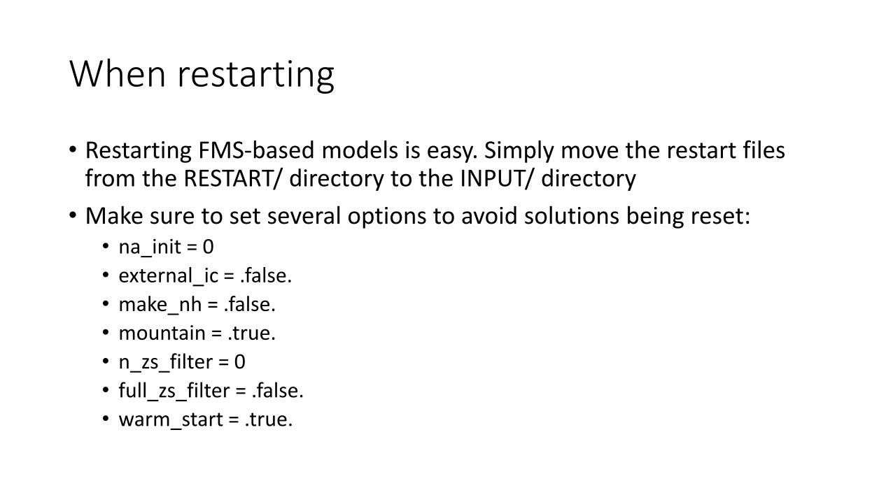
When restarting

• Restarting FMS-based models is easy. Simply move the restart files from the RESTART/ directory to the INPUT/ directory

• Make sure to set several options to avoid solutions being reset:• na_init = 0

• external_ic = .false.

• make_nh = .false.

• mountain = .true.

• n_zs_filter = 0

• full_zs_filter = .false.

• warm_start = .true.

Grid refinement (preview)FV3 supports both stretching and nesting for grid refinement

Grid stretching is simple and smooth Grid nesting is efficient and flexible

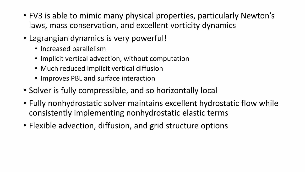
• FV3 is able to mimic many physical properties, particularly Newton’s laws, mass conservation, and excellent vorticity dynamics

• Lagrangian dynamics is very powerful!• Increased parallelism

• Implicit vertical advection, without computation

• Much reduced implicit vertical diffusion

• Improves PBL and surface interaction

• Solver is fully compressible, and so horizontally local

• Fully nonhydrostatic solver maintains excellent hydrostatic flow while consistently implementing nonhydrostatic elastic terms

• Flexible advection, diffusion, and grid structure options