the stability of three- wheeled vehicles & · pdf filethe stability of three- wheeled...

Worcester Polytechnic Institute | Error! No text of specified style in document. 0

Major Qualifying Project

The Department of

Mechanical Engineering

Worcester Polytechnic

Institute

2012

THE STABILITY OF THREE- WHEELED VEHICLES & TWO WHEEL BICYCLES

DMITRI LURIE

Worcester Polytechnic Institute | MQP 2012. D. Lurie 1

Table of Contents

Abstract .................................................................................................................................................... 2

1. Motorcycle with a Sidecar ....................................................................................................... 3

1.1 Directional Stability ......................................................................................................................... 3

1.2 Rollover instability .......................................................................................................................... 6

2. Self-Stability of a Bicycle ........................................................................................................ 7

2.1 Statement of the problem .............................................................................................................. 7

2.2 Method ........................................................................................................................................... 8

2.3 Results ........................................................................................................................................... 10

3. Controlled Stability of a Bicycle ........................................................................................ 12

Conclusions .......................................................................................................................................... 14

References ............................................................................................................................................ 15


Acknowledgements

I wish to thank my advisor, Professor Christopher Scarpino, for his patience, good advice, and

major assistance that I received from him during my work on this project. My thanks go to Professor

Mihhail Berezovski for his invaluable assistance providing the graphics and formatting for this report.


Abstract

The goal of this project is the investigation of the stability of several non-trivial transportation devices,

such as a motorcycle with a sidecar and a two-wheel bicycle, under various dynamic conditions.

The first approach is a theoretical study of the stability in the motion of a motorcycle with a sidecar. Its

specific feature is its lack of symmetry. In the project, conditions were obtained that guarantee directional,

lateral, and, most importantly, rollover stability. Under certain dynamic conditions, tipping may be

possible about a line through the ground contacts of the side wheel and the front or rear wheels.

In this problem, stabilization is permanently fixed through design choices and manufacturing expertise.

The project also studies the dynamic control maintained over a bicycle through the course of its motion.

The first dynamic topic concerns the self-stability of a bicycle where the gyroscopic effects have been

removed. The problem is more than a century old, but only recently (2011) has it been realized that an

uncontrolled bicycle without any gyro effects can demonstrate self-stability due to an appropriate

feedback applied through the steering column alone. In this project, the values of some constructive

parameters were determined that maximize the forward velocity range for uncontrolled stability.

The second dynamic topic of the project concerns the controlled stability of a moving bicycle. Its vertical

position is then maintained via special action taken by a rider who properly operates the handlebar. A

bicycle is similar to an inverted pendulum acted upon by an additional force created through rotation of

the handlebar. The main idea is to operate the handlebar so as to make this force identical to the force that

appears when fast vertical oscillations of a pivot stabilize an inverted pendulum. As a consequence, the

bicycle can be stabilized for forward velocities above a certain limit.


1. Motorcycle with a Sidecar

There is some literature [1,2] on the theoretical analysis of stability for symmetric tricycles, such as the

delta and tadpole motorcycles (Fig.1).

Figure 1. Top and rear view of delta (left) and tadpole (right) tricycle models

In this project, we consider, as an alternative, a sidecar motorcycle outfit. Unlike delta and tadpole, this

outfit is lacking symmetry, which affects its directional and lateral stability. To the best of our knowledge,

the stability analysis has not been conducted for a non-symmetric case. In the following section we are

providing an analysis of the directional stability of a sidecar outfit negotiating a turn.

1.1 Directional Stability

A scheme for the sidecar vehicle is given in Fig. 2.

Figure 2. Schematic model of the sidecar outfit


Weights applied to wheels are designated as (index 1 for front wheel F, index 2 for rear wheel

R, and index 3 for side wheel S); .

Usually, the coordinates of wheels are known, whereas the coordinates of the CoG depend on the

distribution of weight among the wheels, that is, upon two independent parameters. The lateral forces ,

, are linked with the slip angles (Fig. 2) by the formulae:

with stiffnesses . Here, we assume that the two planes through the rear wheels and side wheels

remain parallel to each other. Also, is assumed to be constant and significantly larger than the

contribution due to rotational velocity Differential equations of motion take the form [1,2]:

where is the moment of inertia about CoG, and the symbols a1,..,a4 are combinations of lateral

stiffnesses. The geometric parameters were introduced in Fig. 2., including weight W, and forward

velocity Vx:

From geometry, and by small-angle assumption


A sidecar outfit negotiating a turn is directionally stable, i.e., it isn’t brought to uncontrolled rotation as

long as , or, after transformations,

( )

(1)

where L12= l1+ l2, L13= l1+ l3, L23= l2 - l3.

To study how the weight applied to every wheel affects directional stability, we show in Fig. 3 how the

CoG (point O) splits the triangle 123 into three triangles 203, 103 and 102. Each is proportional,

respectively, to the weights W1, W2, W3.

Figure 3. Location of the Center of Gravity

Directional stability will take place regardless of Vx if the factor of in (1) is negative, that is,

( ) ( ) (2)


This means that a sufficient load on the front and side wheels guarantees directional stability for any Vx. If

(2) is violated then this stability will be preserved if Vx2 remains below the critical value

(3)

1.2 Rollover Instability

The sidecar outfit may also demonstrate rollover instability as a result of lateral acceleration caused for

any reason (e.g., a wind gust), but also while it is accelerating or breaking in a turn. An accident or

rollover may occur either about the axis 3-1 or about the axis 2-3 in Fig. 3. For example, when lateral

acceleration a applies perpendicular to the line 2-1 then no rollover happens if

.

Here, H is the height of the CoG over the ground. If a rollover occurs, then it will require less acceleration

to happen around the 3-1 axis if

The smaller is the load m2 on the rear wheel, and the closer are the axes 2 and 3 to coincidence, the easier

will be the chance of a turnover about the line 3-1.

2. Self-Stability of a Bicycle

2.1 Statement of the problem

While a bicycle is a complicated mechanical assembly, its structure does allow for satisfactory modeling.

For schematic versions, see Figs. 4 and 5 [3]. The tilt angle (positive or negative) for the steering axis is

given by . In this model, the wheels are replaced by skates (“two-mass-skate” bicycle - TMS), which is

reasonable if the gyro effect is removed thanks to a compensating wheel mounted on the frame. This

removal was purposefully introduced in [3] to eliminate the stabilizing action of gyro effect and to

determine how the steering wheel alone would work as a stabilizing factor. The differential equation

[ ]


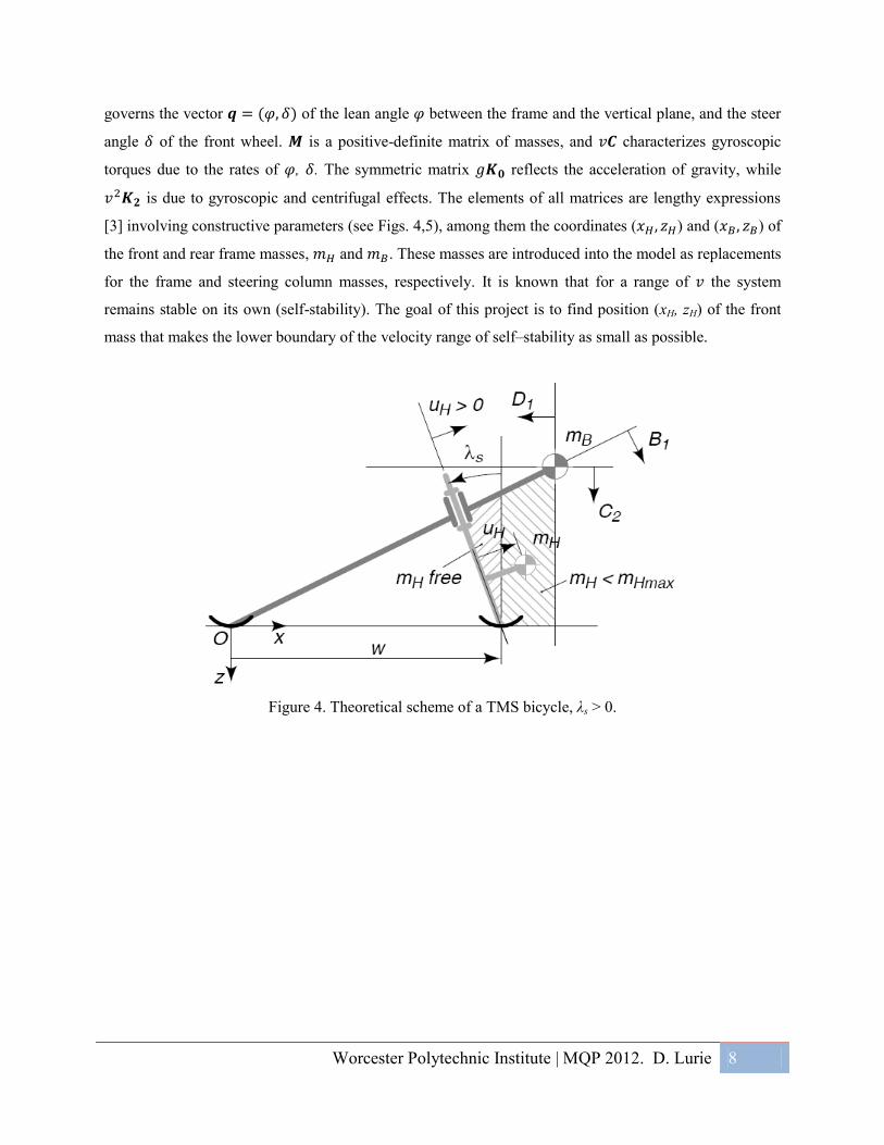
governs the vector of the lean angle between the frame and the vertical plane, and the steer

angle of the front wheel. is a positive-definite matrix of masses, and characterizes gyroscopic

torques due to the rates of , . The symmetric matrix reflects the acceleration of gravity, while

is due to gyroscopic and centrifugal effects. The elements of all matrices are lengthy expressions

[3] involving constructive parameters (see Figs. 4,5), among them the coordinates ( ) and ( ) of

the front and rear frame masses, and . These masses are introduced into the model as replacements

for the frame and steering column masses, respectively. It is known that for a range of the system

remains stable on its own (self-stability). The goal of this project is to find position (xH, zH) of the front

mass that makes the lower boundary of the velocity range of self–stability as small as possible.

Figure 4. Theoretical scheme of a TMS bicycle, λs > 0.


Figure 5. Theoretical scheme of a TMS bicycle, λs < 0.

2.2 Method

We apply Routh-Hurwitz (RH) criterion that guarantees the negativeness of the real parts of all roots of

the characteristic equation

An equivalent form for it

(4)

introduces the symbols defined as

, , ,

, . (5)

The coefficients in these expressions are functions of material properties and constructive

parameters [3], among them ( ). The RH criterion requires that all coefficients A, B, C, D, E, and the

polynomial

should be negative. These conditions are

tested below for both schemes represented in Figs. 4 and 5, and optimal locations ( ) and the

smallest critical velocities found for these schemes. The following formulae for are given in [3]:


,

, (6)

,

,

,

Here and below, the symbols and have the following meaning:

, (7)

The RH inequalities now become (notice that both are negative):

(i) ;

(ii) for , that is,

either and

or , and

(iii) , that is,

either , and ,

or , and ;

(iv) , that is,

either , and ,

or , and ;

(v) , that is,

either , and ,

or , and .

We see that inequalities take place simultaneously for both positive

and negative values of .


By (7), the formula (6) for is rewritten as [ ]. To

guarantee it is necessary that For positive , this means . In other words,

for a structure where the steering is in the “leaned back” orientation, the front mass should be in front of

the steering axis. For positive values of , we have, by (ii) – (iv), and , and

. The first of these inequalities means that the front mass is below a line through O and the

rear mass (Fig. 4). Another two inequalities say that the shaded domain shown in Fig. 4 is consistent

with (ii) – (iv). As to (v), this inequality is satisfied for all if this mass is within the triangle in the

portion of the shaded domain to the left of . When we go to the rest of the shaded domain, then

inequality (v) is satisfied only for

The RH conditions are now reduced to

, and

(8)

These inequalities determine the critical velocity at which the bicycle loses stability. We give the

numerical analysis in the following section. Specifically, we will be interested in the position ( ) of

the front mass that makes the critical velocity as low as possible.

2.3 Results

In Fig. 4, we assign the following parameters: , , ,

. The coefficients A, B, D, E are all positive for if ( ) falls into the shaded domain

in Fig. 4. Adjusting the data for Fig. 4, we specify the parameters as: , , ,

, . The coefficients A, B, D, E are all positive for with

( ) inside the shaded domain in Fig. 5. Because in both cases, the optimal critical value of

is defined by (8) as

[ (

)]

The ratios – and – depend on ( ) taking values within the shaded regions. The graphs

of the ratios (red for – and blue for – ) are reproduced in Fig. 6a for positive , and in

Fig. 6b for negative . We see that in both cases, the blue surface is above the red one, so it is the ratio

– that defines the critical velocity below which stability is lost.


When (see Fig. 4), the minimum critical velocity of 2.26 is attained at and

. That is, when the load is mounted on the front skate. Using (xH, zH) = the

non-optimal critical velocity was found in [3] to be 2.8 .

When (see Fig. 5), the minimum critical velocity of 2.16 is attained at ( ) = ( ).

That is, when the front mass and the frame mass are located at the same point. Using ( ) =

, the non-optimal critical velocity was found in [3] to be 2.6 .

Figure 6a. Plot of – (red) and – (blue) as function of ( ) for .

Figure 6b. Plot of – (red) and – (blue) as function of ( ) for .


3. Controlled Stability of a Bicycle

A simple model of a bicycle assumes that for a tilt angle the CoG of the front assembly will be

located on the steering column. The front assembly is defined as the front wheel, the front forks and the

handlebar. The rear assembly includes the frame, plus the rider, the rear forks and the rear wheel. For this

typical arrangement, the lean and the steer angles satisfy the equation [4]

( ) (9)

The coefficients then have the following meaning:

The following symbols define the configuration of the bicycle. Through we denote, respectively,

the central moment of inertia of the rear assembly relative to the horizontal axis, and the mixed central

moment of inertia relative to this axis and the axis perpendicular to it in the plane of the rear wheel. The

symbols denote the similar moments for the front assembly. are the moments of inertia of

the rear (front) wheels about their axes of rotation; are the distances from the CoG of the rear

(front) wheels to the ground; are the masses of the assemblies. The symbols denote the

horizontal distances between the ground contact of the rear wheel and the horizontal projections of the

CoG of the rear (front) assemblies. The symbol is, as before, the base of the bicycle, and is equal to

times the trailing1 distance of the front wheel. Parameter is defined as the shortest distance

between CoG of the front assembly and the steering wheel.

1 As taken from Wikipedia: “Trail, or caster, is the horizontal distance from where the steering axis intersects the ground to where

the front wheel touches the ground.”


Assume that and define ( ) as coordinates of the CoG of the bicycle; then

(here ). Neglecting the moments of inertia compared to ,

where is the wheel’s radius, we reduce Eq. (9) to

(10)

where

and is the forward velocity. The steer angle serves here as a factor controlled by a rider to

maintain stability. The equation (10) is the same as the equation of an inverted pendulum acted upon by

additional force represented by the last three terms on the left hand side. We now introduce the feedback

through defining these terms as

(11)

Eq. (10) then takes the form

(

) (12)

identical with the equation of the inverted pendulum with the pivot subjected to vertical oscillation

. Such oscillation is known to stabilize the pendulum if [5]

√

Eq. (12) is the Mathieu equation, with its solution bounded once the last inequality holds. Now it is

possible to find by integrating (11), and this law should be enforced by the rider operating the

handlebar. The function at the right hand side of (11) is bounded, and the relevant solution has

values that are also bounded. This bound is well-known [6]; it is defined by

| |

Here, is a static deviation of from zero due to the action of the force equal to the maximum value

of the rhs of (11):


with parameters and defined, respectively, as

√

.

We assume here that parameter in (11) is small enough to offer relatively low resistance.


Conclusions

1. The influence of weight distribution on directional stability of a sidecar motorcycle outfit is

examined with the aid of the stability analysis applied to the differential equations governing the

transverse and angular velocity of the vehicle negotiating the turn. The results specify the upper

boundary of the forward velocity below which stability is lost. A similar analysis applies to the

instability under the influence of external acceleration. It specifies conditions under which the

turnover occurs either about the axis connecting the ground contacts of the side and front wheels,

or about the axis between the ground contacts of the side and rear wheels.

2. The study of self-stability of the two-wheeled bicycle establishes conditions that minimize the

critical velocity under which the self-stability is lost. We choose the position of the CoG of the

front assembly as a control parameter, and find the optimal value of this parameter when the tilt

angle of the front wheel is positive as well as negative.

3. Unlike the self-stability mode, the stability of the bicycle controlled by a rider is examined in the

third section. Here, we assume that the rider acts to operate the handlebar such that a bicycle

remains stable. To achieve this, we utilize an effect well-known to every bicycle rider: the

stability is maintained when an oscillatory rotation is applied to the steering wheel. In our

mathematical description, we argue mechanically by treating the bicycle as an inverted pendulum.

An inverted pendulum can be stabilized if its pivot is subjected to high-frequency vertical

oscillations. A similar mechanism works for the case of a bicycle where rotation of the handlebar

produces vertical oscillations in the front forks. Using a feedback approach, we identify the

bicycle equation with the equation of an inverted pendulum whose stability is maintained via an

oscillating pivot. From this, we obtain the rule for operating the handlebar dictated by the lean

angle at each instance of time, and the upper bound of the handlebar’s oscillation is determined.


References

[1] Wong, J.Y, Theory of Ground Vehicles, Wiley (2008).

[2] Huston, J.C., Graves, B.J., and Johnson, D.B., Three Wheeled Vehicle Dynamics, SAE Technical

Paper 820139: 45-58 (1982).

[3] Kooijman et al., A Bicycle Can Be Self-Stable Without Gyroscopic or Caster Effects, Science 332

(6027): 339-342 (2011); supporting online text material:

www.sciencemag.org/cgi/content/full/332/6027/339/DC1.

[4] Neimark, Ju. I., Fufaev, N.A., Dynamics of Nonholonomic Systems, Volume 33 of Translations of

Mathematical Monographs, AMS (1972).

[5] Panovko, Ya.G., An Introduction to the Theory of Mechanical Oscillations (in Russian), Nauka,

Moscow (1980).

[6] Loitsianskii, L.G., and Lurie, A.I., A Course in Theoretical Mechanics (in Russian), Drofa, Moscow

(2006).

the stability of three- wheeled vehicles & · pdf filethe stability of three- wheeled...

Documents