the spectrum of the cubic oscillator

Digital Object Identifier (DOI) 10.1007/s00220-012-1559-zCommun. Math. Phys. 319, 479–500 (2013) Communications in

MathematicalPhysics

The Spectrum of the Cubic Oscillator�

Vincenzo Grecchi, André Martinez

Dipartimento di Matematica, Università di Bologna, Piazza di Porta San Donato, 40126 Bologna, Italy.E-mail: [email protected]; [email protected]

Received: 11 January 2012 / Accepted: 15 February 2012Published online: 30 August 2012 – © Springer-Verlag 2012

Abstract: We prove the simplicity and analyticity of the eigenvalues of the cubic oscil-lator Hamiltonian,

H(β) = − d2

dx2 + x2 + i√βx3,

for β in the cut plane Cc := C\R−. Moreover, we prove that the spectrum consists of theperturbative eigenvalues {En(β)}n≥0 labeled by the constant number n of nodes of thecorresponding eigenfunctions. In addition, for all β ∈ Cc, En(β) can be computed asthe Stieltjes-Padé sum of its perturbation series at β = 0. This also gives an alternativeproof of the fact that the spectrum of H(β) is real when β is a positive number. This way,the main results on the repulsive PT-symmetric and on the attractive quartic oscillatorsare extended to the cubic case.

1. Introduction

The real cubic oscillator,

H = − d2

dx2 + x2 + x3, (1.1)

has been considered from the very beginnings of quantum mechanics as one of the sim-plest operators to study (see, e.g., [8]). Indeed, it is the simplest model after the two casesof a linear potential and a quadratic potential. But, in contrast with these two models (forwhich Airy and Weber functions can be used), no general analogous special functionsare known for the cubic case (see, however, [6]). In addition, from a quantum point ofview, it appears that there exists an infinity of self-adjoint extensions from C∞

0 (R), all

� Partly supported by Università di Bologna, Funds for Selected Research Topics.

480 V. Grecchi, A. Martinez

with discrete spectrum (see, e.g., [21] for such considerations). Therefore, this apparentsimplicity actually hides important difficulties, for which a rigorous treatment is needed.

Here, in order to get a better understanding of the problem, we consider the complexHamiltonian,

H(β) = − d2

dx2 + x2 + i√βx3, (1.2)

where β �= 0 is a complex parameter with | argβ| < π . In particular, for positive β,H(β) is PT-symmetric, as the repulsive quartic oscillators defined and studied in [4].

Strangely enough, until recently there were rather few rigorous published resultsconcerning this operator. Among them, however, we can quote the analyticity of theeigenvalues for small |β| and the Borel summability [6], extended to the boundaryarg(β) = ±π, as distributional Borel summability [5].

On the contrary, many papers have been devoted to the quartic anharmonic oscillator(see, e.g., [4,13,19,20,24,27]), for which a rather complete series of results have beenproved.

Indeed, a renewed interest for this model came only after the Bessis-Zinn Justin con-jecture in 1992 (successively extended to other oscillators by Bender-Boettcher in [2],after the results of [4] on the quartic oscillator), claiming that the spectrum of H(β)should be real for positive β. After an important step due to Dorey-Dunning-Tateo in[12], the conjecture was finally proved by Shin in [22] (actually for a more general classof Hamiltonians).

In this paper, we recover Shin’s result in our case, but with a completely differentproof. In addition, our proof permits us to give complete information on the spectrumof H(β) for all β in the cut plane.

More precisely, we prove that the spectrum of H(β) consists of the perturbativesimple eigenvalues {En(β)}n≥0, labeled by the constant number n of the nodes of thecorresponding eigenfunctions, that is, its zeros lying in the lower half-plane (that arestable in the β = 0 limit). In addition, we prove that, for all β such that | argβ| < π ,each eigenvalue En(β) is the Stieltjes-Padé sum of its perturbation series at β = 0. Inthis way we extend to the cubic case the results by Loeffel-Martin-Simon-Wightman[19] on the quartic oscillator (see also [24]).

Our method, that we believe to be new, is based on a combined use of perturbativeand complex semiclassical arguments. In particular, it exploits in an intensive way thestability of the nodes of the eigenfunctions when the energy tends to infinity. More pre-cisely we prove that, for any eigenfunction depending continuously on β, its number ofnodes is indeed independent of β and remains uniformly bounded. On the other hand,semiclassical considerations show that this number is related to the value of the energyand, in particular, tends to infinity as the energy tends to infinity. This shows that theenergy cannot explode for finite β (even in the limit argβ → ±π ), and permits us toobtain global results. A similar strategy has been used by Loeffel and Martin [20] forthe anharmonic quartic oscillator, with the difference that, in their case, the particularform of the potential allowed the use of variational inequalities, leading to the result ina much simpler way.

Let us observe that the limit of En(−b−iε) as ε → 0+, gives a generalized resonanceof (1.1) defined as the limit of resonances of analytically regularized Hamiltonians [7].

A general discussion on the problem, extended to the non-modal solutions, has alsobeen presented in two recent papers in collaboration with Marco Maioli [15,16] (but thecontrol on the non-perturbative levels was not complete).

The Spectrum of the Cubic Oscillator 481

Finally, in relation with our result, we would like to mention the complex semiclassicalstudies by Eremenko-Gabrielov-Shapiro [14], Delabaere-Pham [9,10] and Delabaere-Trinh [11] (see also [26] and references therein), and the numerical computations doneby Bender & Weniger [3], G. Alvarez [1] and Zinn-Justin & Jentschura [29,30].

In the next section, we describe our main results and make some general remarkson them. Section 3 is devoted to some preliminary results concerning any arbitraryeigenvalue E(β) of H(β), depending continuously on β in some open set � ⊂ Cc. Inparticular, it is shown that the corresponding eigenfunction admits a finite number ofzeros (nodes) in the half-plane {Im x < 0}, and that this number is independent of β.Using this property, we show that E(β) can be continued (as an eigenvalue of H(β))along any simple path of Cc. In Sect. 4, we consider the particular case where the pathrelates � with 0, and we prove that, when β becomes close to 0, then E(β) can beidentified with some perturbative eigenvalue En(β). The simplicity of the eigenvaluesis proved in Sect. 5 where, still using the properties of the nodes of the eigenfunctions,we show that each En(β) can be continued in a holomorphic way to the whole cut plane.Then, in order to have the Stieltjes property, we study the behavior of En(β) both whenβ becomes close to the cut and when |β| tends to infinity. In particular, we show thatEn(β) admits a finite limit E±

n (−b) as β → −b ∈ (−∞, 0)with ± argβ < π (Sect. 6),and that En(β) behaves like β1/5 as |β| → ∞ (Sect. 7). This permits us, in Sect. 8, toprove that the function β−1(En(β) − En(0)) is Stieltjes, and to complete the proof ofour results.

2. Results

We study the spectrum of the non-selfadjoint operator,

H(β) := − d2

dx2 + x2 + i√βx3 (2.1)

on L2(R), for β ∈ Cc := C\(−∞, 0] and with domain,

D := {u ∈ H2(R) ; x3u(x) ∈ L2(R)},where H2(R) stands for the usual Sobolev space of index 2 on R.

It is well known (see, e.g., [6]) that, forβ ∈ Cc, H(β) forms an analytic family of typeA (in the sense of Kato [18]) with compact resolvent, and that, for any θ ∈ (−π, π), theoperator H(beiθ ) tends to H0 := − d

dx2 +x2 (with domainD0 := {u ∈ H2(R) ; x2u(x) ∈L2(R)}) in the norm-resolvent sense, as b → 0+.

Moreover, denoting by En(0) = 2n + 1 (n ≥ 0) the (n + 1)th eigenvalue of H0, onecan see ([6], Thm. 2.13 and [5]) that, for all n ≥ 0, there exists δn > 0 such that, for anyβ ∈ Cc with |β| < δn , one has,

σ(H(β)) ∩ {|z − En(0)| < δn} = {En(β)}, (2.2)

where En(β) is a simple eigenvalue depending analytically on β and bounded on Cc ∩{|β| < δn}. Finally, En(β) admits an asymptotic expansion as β → 0 (β ∈ Cc), of theform,

En(β) ∼ En(0) +∑

k≥1

en,kβk, (2.3)


where all the coefficients en,k are real, are given by the Rayleigh-Schrödinger perturba-tion theory, and satisfy the estimate,

|en,k | ≤ DnCkn k! (k ≥ 0), (2.4)

where Cn and Dn are positive constants. (Actually, it is proved in [6,5] that the previousseries is Borel summable to En(β) when | argβ| < 3π

4 − ε, ε > 0 arbitrary, |β| smallenough, and more generally, in the distributional sense for the other values of argβ;however, here we will not use these results.)

Here, we prove,

Theorem 2.1. For all β ∈ Cc, the spectrum σ(H(β))of H(β) consists of simple eigen-values En(β) (n = 0, 1, ...) depending analytically on β ∈ Cc. Moreover, for all β ∈ Ccand n ≥ 0, one has,

En(β) = En(0) + β limj→+∞

Pn, j (β)

Qn, j (β), (2.5)

where Pn, j and Qn, j are the polynomials of degree j (“diagonal Padé approximants”)defined by,

⎧⎨

⎩

Qn, j (0) = 1;∣∣∣

Pn, j (β)

Qn, j (β)− ∑2 j

k=1 en,kβk∣∣∣ = O(|β|2 j+1) as β → 0.

Actually, one point of the proof will consist in showing that the series (|en,k |)k≥1 isStieltjes (see, e.g., [28] for a definition). In particular, its diagonal Padé approximantssatisfying the condition Qn, j (0) = 1 are well defined and unique (see [28], Chap. XX).Indeed, we also prove,

Theorem 2.2. For all β ∈ Cc, one has,

En(β) = En(0) + β∫ +∞

0

ρn(t)

1 + βtdt,

where ρn is a real-analytic positive function on (0,+∞), such that t1/5ρn(t) admits alimit as t → 0+, and,

ln ρn(t) = − 8

15(t + O(ln t)), as t → +∞.

Moreover, the measure ρn(t)dt is the only solution of the moment problem,∫ +∞

0tkρn(t)dt = |en,k+1| (k = 0, 1, . . . ).

In particular, the constant Cn in (2.4) can be taken arbitrarily close to 15/8.

Remark 2.3. By the results of Sibuya [23], we already know that, for β ∈ Cc fixed, thelarge enough eigenvalues of H(β) are simple. However, no information is given in [23]about how large they must be (in particular when β becomes close to infinity or to theboundary of Cc). Moreover, still by [23], one can see that any eigenspace Ker(H(β)−E)is one dimensional (that is, the geometric multiplicity of E is one). Therefore, the pos-sible (algebraic) multiplicity of an eigenvalue necessarily means the appearance of nonvanishing Jordan blocks.


Remark 2.4. When β is a positive number, the operator H(β) is PT-symmetric and thereality of its spectrum is proved by Shin in [22]. Here, we can recover this result e.g. byobserving that, since all the en,k are real, so are all the coefficients of Pn, j and Qn, j . Butin fact, the reality of En(β) is not related to the Padé summability, but is rather a directconsequence of its simplicity and of its characterization by the number of nodes of theassociated eigenfunction (see Definition 3.5, Proposition 3.6 and (6.1)).

Remark 2.5. In particular, it follows from this theorem that all the eigenvalues of H(β)are holomorphic extensions to the whole cut plane Cc of the perturbative eigenvaluescomputed near β = 0.

3. Preliminaries

We start with some general results concerning the eigenvalues of H(β).By the results of [18] and [23], we know that, if E0 is an eigenvalue of H(β0) for

some β0 ∈ Cc, then its multiplicity m is finite and there exists an integer m′ ∈ [1,m] anda m′-valued analytic function β �→ E(β) defined on a neighborhood of β0 with branchpoint at β0, such that E(β) → E0 as β → β0, and E(β) is an eigenvalue of H(β) forall β in this neighborhood.

In other words, the function β �→ E(β) is well-defined and analytic on the m′-sheetscovering space over�\{β0}, where� is a neighborhood of β0 in Cc, and moreover it iscontinuous at β0.

Let us note that, by the results of [23], the algebraic multiplicity of E0 coincides withits multiplicity as a zero of the Stokes-Sibuya coefficient (see, e. g., [26]). In particular,the finitude of m is a direct consequence of the global analyticity of this coefficient withrespect to the energy.

The purpose of this section is to continue holomorphicaly any of the branches ofE(β), in order to reach any point of Cc (in particular, points arbitrarily close to 0). Atfirst, we prove,

Proposition 3.1. There exists a L2(R)-multiple-valued continuous function ψβ of β ∈�, such that, for all β ∈ �, one has H(β)ψβ = E(β)ψβ and ‖ψβ‖ = 1.

Proof. For E ∈ C, denote by ψ±,E the two solutions of H(β)ψ±,E = Eψ±,E that aresubdominant near R± respectively, and are given by the Sibuya asymptotics (see [23],Chap. 2). In particular, ψ±,E are L2(R±)-valued analytic functions of (E, β), and thefact that E(β) is an eigenvalue of H(β) means that there exists a complex number αβsuch thatψ+,E(β) = αβψ−,E(β). Moreover, sinceψ−,E (z) is a non identically zero entirefunction of z, for any nonempty open set ω ⊂ C, one has ‖ψ−,E‖L2(ω) �= 0. Thus, onecan write αβ = 〈ψ+,E(β), ψ−,E 〉L2(ω)/‖ψ−,E‖2

L2(ω), showing that αβ is a continuous

function of β. As a consequence, so is ‖ψ+,E(β)‖2 = ‖ψ+,E(β)‖2R+

+ |αβ |2‖ψ−,E(β)‖2R− ,

and the function ψβ := ψ+,E(β)/‖ψ+,E(β)‖ solves the problem. ��Remark 3.2. Actually, by the results of [23], we know that αβ can be expressed asαβ = C(

√β, E(β)), where the function C

2 � (α, E) �→ C(α, E) is entire.

Next, we prove,

Proposition 3.3. For all β ∈ �, the eigenfunction ψβ does not admit any zero in thestrip,

Sβ :={

x ∈ C ; 0 ≤ Im x ≤ 2

3√|β| cos(

argβ

2)

}.


Proof. Setting Vβ(x) := x2 + i√βx3, and using the equation, we see that, for any

s, t ∈ R, we have,

Im ψ ′β(s + i t)ψβ(s + i t) =

∫ s

−∞Im (Vβ(r + i t)− E(β))|ψβ(r + i t)|2dr

= −∫ +∞

sIm (Vβ(r + i t)− E(β))|ψβ(r + i t)|2dr. (3.1)

Therefore, it is enough to prove that, for 0 ≤ t ≤ 23√|β| cos( argβ

2 ), the function r �→Im (Vβ(r + i t) − E(β)) changes sign at most once on R (in that case, at least one –and thus both – of the two previous integrals is necessarily different from zero). Writingβ = beiθ with b > 0 and |θ | < π , we compute,

d

drIm Vβ(r + i t) = d

dr

(2r t + r3

√b cos

θ

2− 3r2t

√b sin

θ

2− 3r t2

√b cos

θ

2

)

= 3r2√

b cosθ

2− 6r t

√b sin

θ

2+ 2t − 3t2

√b cos

θ

2.

This is a second order polynomial function of r , with (reduced) discriminant given by,

�′ = 9t2b − 6t√

b cosθ

2= 3t

√b(3

√bt − 2 cos

θ

2).

In particular, this discriminant is non positive when 0 ≤ t ≤ 23√

bcos θ2 , and the result

follows. ��Proposition 3.4. There exists C(β) > 0, depending continuously on β ∈ �, such thatthe eigenfunction ψβ does not admit any zero in the set,

{x ∈ C ; Im x < 0 , |x | ≥ C(β)}.Proof. This is just an immediate consequence of the Sibuya asymptotics at infinity ofψβ(x), in the two sectors,

S± := {x ∈ C ;∣∣∣∣arg(i x) +

argβ

10∓ 2π

5

∣∣∣∣ <

3π

5}, (3.2)

(see [23], Chap. 2). Since S+ ∪S− = C\(ei( π2 + θ10 )R+) ⊃ {Im x < 0}, the result follows.

��We deduce from Propositions 3.3 and 3.4 that, for any continuous function C(β) ≥

C(β), the number of zeros of ψβ lying in the region,

�β := {Im x ≤ 2

3√|β| cos(

argβ

2) , |x | ≤ C(β)}

is constant. Indeed, the two previous propositions show that the boundary ∂�β of �β doesnot contain zeros, and thus the number of zeros in �β (finite, because of the analyticityof ψβ ) is given by,

Nβ = 1

2iπ

∮

∂�β

ψ ′β(x)

ψβ(x)dx = 1

2iπ

∮

∂�β

ψ ′β(x)

ψβ(x)dx < ∞. (3.3)


In particular, this number is a continuous function of β, and therefore is constant forβ ∈ �. Moreover, still by Propositions 3.3 and 3.4, these zeros are the only ones in{Im x ≤ 2

3√|β| cos( argβ

2 )}. At this point, it will be useful to set,

Definition 3.5. For any eigenfunction ψ of H(β), we call a node of ψ any zero of ψthat lies in the lower half-plane C− := {Im x < 0}, and we denote by N (ψ) their totalnumber.

The previous discussion shows that we have,

Proposition 3.6. N (ψβ) is finite and does not depend on β ∈ �. Moreover, the nodes

of ψβ coincide with its zeros in the domain {Im x ≤ 23√|β| cos( argβ

2 )}, and their total

number can be computed by using the formula (3.3).

From now on, we denote by Nψ the total number of nodes of ψβ for any β ∈ �.In the following, we will also need a better control of the zeros in the region {Im x >

0}. We have,

Proposition 3.7. The function ψβ does not admit any zero in the region,

{0 < arg x <π − argβ

10} ∪ {π − π + argβ

10< arg x < π}.

Proof. By (3.1) for s = t = 0, we see that Im ψ ′β(0)ψβ(0) < 0. Moreover, since ψβ is

subdominant in both sectors S±1(β) defined by,

S j (β) := {x ∈ C ;∣∣∣∣arg(i x) +

argβ

10− 2 jπ

5

∣∣∣∣ <

π

5}, j = ±1, (3.4)

we see that, for α ∈ (0, (π − argβ)/10), the function s �→ ψβ(seiα) is in L2(R+).Therefore, for s > 0, using the equation H(β)ψβ = E(β)ψβ , we obtain,

Im ψ ′β(seiα)ψβ(seiα) = Im ψ ′

β(0)ψβ(0) +∫ s

0pα(r)|ψβ(reiα)|2dr

= −∫ +∞

spα(r)|ψβ(reiα)|2dr,

with,

pα(r) := Im (r2e4iα + i√βr3e5iα − E(β)e2iα)

= r2[

sin 4α + r cos(5α +argβ

2)

]− Im (E(β)e2iα).

In particular, since both sin 4α and cos(5α + argβ2 ) are positive, pα(r) changes sign at

most once on R+, and is positive for large r . We deduce that Im ψ ′β(seiα)ψβ(seiα) < 0

for all s > 0.In the same way, one finds Im ψ ′

β(seiα)ψβ(seiα) < 0 when s < 0 and π − α ∈(0, (π + argβ)/10), and the result follows. ��

Now, we plan to extend continuously the function E(β) as much as possible, as aneigenvalue of H(β). We first show,


Proposition 3.8. The function � � β �→ E(β) is uniformly bounded.

Proof. By contradiction, assume there exists a sequence (βk)k≥0 in � such that|E(βk)| → ∞ as k → ∞. By extracting a subsequence, we can also assume that(βk)k≥0 admits a limit β∞ = b∞eiθ∞ ∈ ∂�, with b∞ > 0 and θ∞ ∈ [−π, π ].

In the equation H(βk)ψβk (x) = E(βk)ψβk (x), we make the (complex) change ofvariable,

x = |E(βk)|1/3e−iθk/10 y,

where we have used the notation θk := argβk ∈ (−π, π). Then, setting,

h := |E(βk)|−5/6; λ := E(βk)e−iθk/5

|E(βk)| ;

P := −h2 d2

dy2 + i√|βk |y3 + h2/5e−iθk/5 y2,

(3.5)

we see that the new function ϕ(y) := ψβk (|E(βk)|1/3e−iθk/10 y) is a solution of,

Pϕ(y) = λϕ(y). (3.6)

Moreover, since ψβ is subdominant in both sectors S±1(β) defined in (3.4), we observethat the function ϕ is automatically exponentially small at infinity on R (and, actually,even in the limit | arg θk | → π ). In particular, it is an eigenfunction of P in the usualsense, and, as k → ∞, we have h → 0+, |βk | → b∞ > 0, θk → θ∞, and λ stayson the circle {|λ| = 1}, with Re λ > 0 (since Re P = −h2 d2

dy2 + h2/5 y2 cos(θk/5) ≥h6/5√cos(θk/5) > 0). By extracting a subsequence, we can also assume that λ = λ(h)admits a limit λ0.

Then, we can try to use the standard semiclassical complex WKB method, in orderto obtain another estimate on the number of nodes of ψβk .

Since Re λ > 0, we see that, among the three turning points (that is, the complex solu-tions of i

√|βk |y3 + h2/5e−iθk/5 y2 = λ), exactly two of them (say, y±(λ)) are in the half-plane {Im y < Ch2/5} (C > 0 constant) and are respectively close to b−1/6∞ ei(2 arg λ−π)/6and b−1/6∞ ei(2 arg λ−5π)/6, while the third one y(λ) is close to b−1/6∞ ei(2 arg λ+3π)/6.

Moreover, each of these points gives rise to three anti-Stokes lines, delimiting threecomplex open sectors. In particular, the sectors attached either to y+(λ) or to y−(λ)are six. In addition, any anti-Stokes line is either bounded (in which case it relates twodifferent turning points) or asymptotic at infinity to one of the five Sibuya directions,given by {arg y = (4 j − 3)π/10}, j = 1, . . . , 5.

Then, for topological reasons related to the properties of the anti-Stokes lines (inparticular, the fact that they cannot cross each other away from the turning points), wesee that at least one of these six sectors necessarily contains either {y ∈ R+ ; y >> 1}or {y ∈ R− ; y << −1}, without containing any other turning point.

Let us assume, for instance, that this open sector (that we denote by �+) is attachedto y+(λ) and contains {y ∈ R+ ; y >> 1} (the other cases are similar). Then, the com-plex WKB method tells us that ϕ(y) �= 0 on �+, and that one has the semiclassicalasymptotics,

ϕ′(y)ϕ(y)

= −1

h

√i√|βk |y3 + h2/5e−iθk/5 y2 − λ + O(1) as h → 0+, (3.7)


locally uniformly with respect to y ∈ �+. Moreover, this asymptotics remains valid inthe two sectors adjacent to �+, as long as one does not cross a third anti-Stokes linecontaining a turning point. In particular, it ceases to be valid at the boundary, say L+,between these two adjacent sectors (near which the zeros of ϕ lie). However, there existsa general estimate on ϕ′/ϕ, valid near L+, too. We describe it in the next lemma.

For any δ > 0 fixed, set,

Eδ := {y ∈ C ; dist(y, ϕ−1(0)) ≥ δh}.Then, we have,

Lemma 3.9. For any δ > 0, one has,

ϕ′(y)ϕ(y)

= O(

1

h

),

locally uniformly for y ∈ Eδ , and uniformly for h > 0 small enough.

This result is probably well-known to semiclassical experts, but for the sake of com-pleteness we give a proof in the Appendix.

Now, we estimate the number of nodes of ϕ lying near y+(λ). By Propositions 3.6and 3.7, we already know that this number is less than Nψ and is bounded uniformlywith respect to h. As a consequence, denoting by W+ a sufficiently small neighborhoodof y+(λ), for any constant δ > 0 arbitrarily small, and for all h small enough, thereexists a point yh ∈ L+ ∩ W+ with (1 + Nψ)δ ≤ |yh − y+(λ)| ≤ (1 + 2Nψ)δ anddist(y, ϕ−1(0)) ≥ δ. We denote by D the disk centered at y+(λ)with radius |yh − y+(λ)|(in particular, if W+ has been chosen small enough, the part of L+ between y+(λ) andyh is included in D, and the boundary ∂D of D is transverse to L+ at yh).

Then, by construction, we have ϕ(y) �= 0 when y ∈ ∂D, and the number of nodesof ϕ lying in D can be written as,

ND = 1

2iπ

∮

∂D

ϕ′(y)ϕ(y)

dy.

For any ε > 0 arbitrarily small, we set,

γ (ε) := ∂D ∩ {|y − yh | ≤ ε} ; �(ε) = ∂D\γ (ε).Since the length of γ (ε) is O(ε), by using Lemma 3.9, we obtain,

ND = 1

2iπ

∫

�(ε)

ϕ′(y)ϕ(y)

dy + O( εh), (3.8)

uniformly with respect to ε and h. On the other hand, since dist(�(ε), L+) ≥ ε, on thisset we can use the asymptotics (3.7), leading to,

∫

�(ε)

ϕ′(y)ϕ(y)

dy =∫

�(ε)

−1

h

√i√|βk |y3 + h2/5e−iθk/5 y2 − λ dy + Oε(1), (3.9)

where the notation Oε(1) means that this quantity depends on ε, and is uniformlybounded as h → 0+.


y

y

Lx

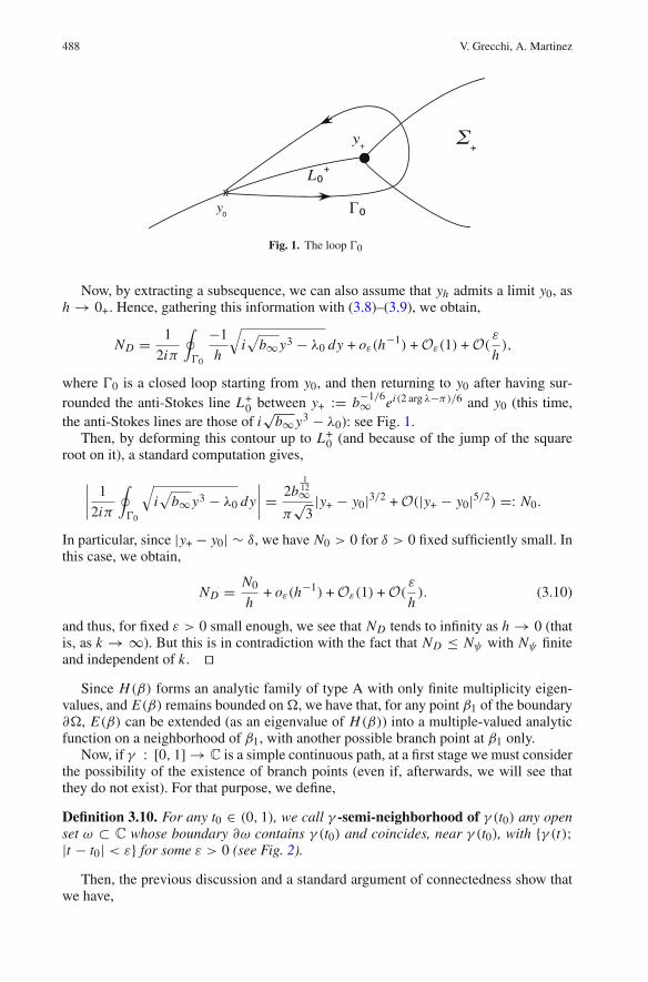
Fig. 1. The loop �0

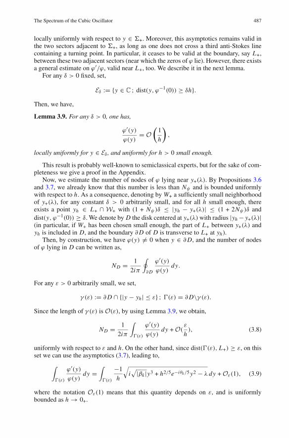
Now, by extracting a subsequence, we can also assume that yh admits a limit y0, ash → 0+. Hence, gathering this information with (3.8)–(3.9), we obtain,

ND = 1

2iπ

∮

�0

−1

h

√i√

b∞y3 − λ0 dy + oε(h−1) + Oε(1) + O( ε

h),

where �0 is a closed loop starting from y0, and then returning to y0 after having sur-rounded the anti-Stokes line L+

0 between y+ := b−1/6∞ ei(2 arg λ−π)/6 and y0 (this time,the anti-Stokes lines are those of i

√b∞y3 − λ0): see Fig. 1.

Then, by deforming this contour up to L+0 (and because of the jump of the square

root on it), a standard computation gives,

∣∣∣∣

1

2iπ

∮

�0

√i√

b∞y3 − λ0 dy

∣∣∣∣ = 2b

112∞

π√

3|y+ − y0|3/2 + O(|y+ − y0|5/2) =: N0.

In particular, since |y+ − y0| ∼ δ, we have N0 > 0 for δ > 0 fixed sufficiently small. Inthis case, we obtain,

ND = N0

h+ oε(h

−1) + Oε(1) + O( εh). (3.10)

and thus, for fixed ε > 0 small enough, we see that ND tends to infinity as h → 0 (thatis, as k → ∞). But this is in contradiction with the fact that ND ≤ Nψ with Nψ finiteand independent of k. ��

Since H(β) forms an analytic family of type A with only finite multiplicity eigen-values, and E(β) remains bounded on�, we have that, for any point β1 of the boundary∂�, E(β) can be extended (as an eigenvalue of H(β)) into a multiple-valued analyticfunction on a neighborhood of β1, with another possible branch point at β1 only.

Now, if γ : [0, 1] → C is a simple continuous path, at a first stage we must considerthe possibility of the existence of branch points (even if, afterwards, we will see thatthey do not exist). For that purpose, we define,

Definition 3.10. For any t0 ∈ (0, 1), we call γ -semi-neighborhood of γ (t0) any openset ω ⊂ C whose boundary ∂ω contains γ (t0) and coincides, near γ (t0), with {γ (t);|t − t0| < ε} for some ε > 0 (see Fig. 2).

Then, the previous discussion and a standard argument of connectedness show thatwe have,


x(t )

Fig. 2. γ -semi neighborhood

Proposition 3.11. Let γ : [0, 1] → Cc\{β0} be an arbitrary simple continuous pathsuch that γ (0) ∈ �. Then, for any determination E(β) of E(β), there exists a finite set{t1, . . . , tk} ⊂ (0, 1), such that E(β) can be extended (as an eigenfunction of H(β)) intoa holomorphic function on W := U ∪ ω1 ∪ · · · ∪ ωk , where U is a complex neighbor-hood of γ \{γ (t1), . . . , γ (tk), γ (1)}, and ω j ( j = 1, . . . , k) is a γ -semi-neighborhoodof γ (t j ). Moreover, the extension is continuous up to the boundary ∂W of W .

In the next section, we relate such an extension with the En(β)’s of (2.2).

Remark 3.1. Actually, the extension can be made in the larger open set obtained byreplacing the γ -semi-neighborhoods by “cut-neighborhoods” of the form ω j\L+

j , whereω j is a neighborhood of γ (t j ), and L+

j = γ (t j ) + z j R+ with z j ∈ C\{0} transverse to

γ at γ (t j ) (in the case of a C1-path). But the previous notion of semi-neighborhoods isenough for our purposes.

4. The Spectrum for Small Parameter

Let γ : [0, 1) → Cc\{β0} be a simple continuous path, such that γ (0) ∈ �, and{γ (t) ; 1 − μ ≤ t < 1} = (0, ν] for some μ, ν > 0.

The previous proposition (applied to γ∣∣[0,1−δ] for any δ > 0) shows the existence

of a (possibly void) countable set {t j ; 1 ≤ j ≤ K } ⊂ (0, 1), with either K < +∞,or K = +∞ and t j → 1 as j → ∞, such that any determination of E(β) in � canbe extended into a holomorphic function on W := U ∪ ω1 ∪ · · · ∪ ωK , where U isa complex neighborhood of γ \{γ (t j ) ; 1 ≤ j ≤ K }, and ω j ( j = 1, . . . , K ) is aγ -semi-neighborhood of γ (t j ).

Still denoting by E(β) such an extension, and with En(β) as in (2.2), we have,

Proposition 4.1. There exists an integer n ≥ 0, such that, for all β ∈ W sufficientlysmall, one has,

E(β) = En(β).

Remark 4.1. In particular, E(β) can be continued analytically in {β ∈ Cc ; |β| < δn},and thus, as a matter of fact, the branch points cannot accumulate at β = 0.

Proof. By construction, W contains a sequence (βk)k≥0 ⊂ (0, ν] that converges to 0.We distinguish two cases.


Case 1. |E(βk)| does not tend to infinity as k → +∞.

In this case, by extracting a subsequence, we can assume that E(βk) admits a finitelimit E0 as k → ∞. But since H(βk) tends to H0 in the norm resolvent sense, wenecessarily have E0 ∈ σ(H0), that is, there exists n ≥ 0 such that E0 = En(0). Using(2.2)-(2.3), we deduce that E(βk) = En(βk) for all k sufficiently large. By the analyticityof E(β) on W , and the simplicity of En(β) (|β| < δn), we conclude that E(β) = En(β)

for all β sufficiently close to some βk (k >> 1), and thus (since En(β) is analytic, too),for all β ∈ W sufficiently small.

Case 2. |E(βk)| tends to infinity as k → +∞.

We separate the elements of the sequence B := (βk)k≥0 in two parts:

P− := {β ∈ B; |E(β)| ≤ β−1}; P+ := {β ∈ B ; |E(β)| ≥ β−1}.When β ∈ P−, we make the change of variable,

x = √|E(β)| y,

and we set,

ϕ(y) := |E(β)| 14ψβ(

√|E(β)| y); h := |E(β)|−1(<< 1)

α := √β|E(β)| ∈ (0, 1]; λ := E(β)

|E(β)| .

Then, we have,

−h2ϕ′′(y) + (y2 + iαy3 − λ)ϕ(y) = 0,

and we can use again complex WKB semiclassical methods. Since β > 0, we haveRe H(β) = H0 ≥ 1 and thus Re E(β) ≥ 1. Therefore, | arg λ| < π/2 and, among thethree turning points, two of them are located in {Im y ≤ 1/

√2}, while the third one is

in {Im y ≥ 1}. Moreover, in this case Proposition 3.3 gives an absence of zeros for ϕin the strip {0 ≤ Im y ≤ 3

2√β|E(β)| }, and thus in {0 ≤ Im y ≤ 1}. Then, an argument

similar to the one leading to (3.10) shows that Nψ tends to infinity as β → 0+, and thisis in contradiction with Proposition 3.6.

Now, when β ∈ P+, we make the change of variable,

x = |E(β)|1/3β1/6 y,

and we set,

ϕ(y) := |E(β)|1/6β1/12 ψβ(

|E(β)|1/3β1/6 y); h := β1/6

|E(β)|5/6 (<< 1),

α := (β|E(β)|)−1/3 ∈ (0, 1]; λ := E(β)

|E(β)| .In this case, ϕ is solution of,

−h2ϕ′′(y) + (αy2 + iy3 − λ)ϕ(y) = 0.

Again, complex semiclassical WKB asymptotics can be used, and we obtain that Nψshould tend to infinity as β → 0+, which is in contradiction with Proposition 3.6. (Letus observe that, by an obvious change of variable, in both cases the turning points canbe deduced from those of y2 + iy3 − λ′, with Re λ′ > 0.) ��


5. Holomorphic Extension

In view of Proposition 4.1, the first part of Theorem 2.1 will follow from the next result.

Proposition 5.1. For any n ≥ 0, the function,

Cc ∩ {|β| < δn} � β �→ En(β)

can be extended to a holomorphic function on the whole cut plane Cc, in such a waythat, for all β ∈ Cc the value at β of the extension (still denoted by En(β)) is a simpleeigenvalue of H(β).

Proof. It is enough to prove that En(β) can be continued, as a simple eigenvalue ofH(β), along any simple continuous path γ : [0, 1] → Cc such that |γ (0)| < δn .

By Proposition 3.11, we already know that En(β) can be extended, as an eigenvalueof H(β), into a continuous function on γ (and, in fact, holomorphic at least on ‘oneside’ of γ ). We set,

t0 := sup{t ∈ [0, 1] ; En(β) is simple at γ (s) for all s ∈ [0, t]}.By contradiction, let us assume t0 < 1.

Since En(β) is continuous along γ , this implies that En(β0) is a multiple eigenvalueof H(β0), where we have set β0 := γ (t0). Hence, because of the analyticity of thefamily H(β), in a neighborhood of β0 the spectrum of H(β) is given either by at leasttwo branches of a multi-valued analytic function around β0, or by at least two differentanalytic functions (see [18], Chap. VII).

In particular, for β in a sufficiently small neighborhood�1 of {γ (t) ; 0 < t0 − t1 <<1}, there exists an eigenvalue E(β), depending analytically on β, such that E(β) �=En(β) for all β ∈ �1, and E(β) → En(β0) as β → β0 (recall that, by definition,En(γ (t)) is simple for t < t0).

On the other hand, by Sects. 3 and 4, we know that E(β) can be extended, as aneigenvalue of H(β), into a holomorphic function on the neighborhood of some simplecontinuous path, arbitrarily close to γ , connecting �1 with a neighborhood of 0, andthat there exists some m ≥ 0 such that E(β) = Em(β) for |β| sufficiently small.

Then, by construction, we necessarily have m �= n, otherwise, by the simplicity (andthus, the analyticity) of En(β) near {γ (t) ; 0 ≤ t < t0}, we would have E(β) = En(β)

on this set.Now, we denote by ψn,β and ψm,β two normalized eigenfunctions associated with

En(β) and E(β) = Em(β), respectively, and depending continuously on β (see Proposi-tion 3.1). By Proposition 3.6, we know that their respective number of nodes, say Nn andNm , do not depend on β. Moreover, since E(β0) = En(β0) and Ker(H(β0)− En(β0))

is one dimensional, we must have ψn,β0 and ψm,β0 co-linear, and thus, necessarily,Nn = Nm . Therefore, in order to obtain a contradiction, it is enough to prove,

Lemma 5.2. For any n ≥ 0, the eigenfunction associated to En(β) (β ∈ Cc, |β| < δn)admits exactly n nodes.

Proof. Denote by ϕn the (n + 1)th normalized eigenfunction of the harmonic oscillatorH0. It is well known that ϕn is holomorphic on C, and admits exactly n zeros that areall located in the real interval In := [−√

En(0),√

En(0)]. Moreover, since H(β) tendsto H0 in the norm resolvent sense as β → 0, and En(0) is simple, the conveniently nor-malized eigenfunction ψn,β associated to En(β) (|β| < δn) converge in norm towards


ϕn as β → 0. By the ellipticity of H0 and H(β) this actually implies that ψn,β − ϕntends to 0 in any Sobolev norm, and thus locally uniformly (together with its derivative).As a consequence, if C is an arbitrarily large positive constant, for all |β| small enoughone has ψn,β(z) �= 0 if C−1 ≤ dist (z, In) ≤ C , and the number N of zeros of ψn,β in{dist (z, In) ≤ C−1} is given by,

N = 1

2iπ

∮

{dist (z,In)=C−1}

ψ ′n,β(x)

ψnβ(x)dx

−→ 1

2iπ

∮

{dist (z,In)=C−1}ϕ′

n(x)

ϕn(x)dx = n (β → 0).

Therefore, N = n and, by Proposition 3.6, these zeros are exactly the nodes of ψn,β .��

It follows from Lemma 5.2 and the previous discussion that t0 = 1, and Proposition5.1 is proved. ��

Putting together Proposition 4.1 and Proposition 5.1, we obtain the fact that, for anyβ ∈ Cc, the spectrum of H(β) is simple, and consists exactly of the holomorphic exten-sions of the perturbative eigenvalues En(β)’s defined for |β| small. In the rest of thepaper, we will prove the last part of Theorem 2.1, that is, the Padé summability of theEn(β)’s. In order to do so, we first need to know the asymptotic behaviours of En(β) asargβ → (±π)∓ and as |β| → ∞.

6. Behaviour on the Cut

From now on, we fix n ≥ 0, and we consider the simple eigenvalue En(β) defined forall β ∈ Cc. We also observe that, since H(β) admits the symmetry,

PT H(β) = H(β)PT ,

(where we have denoted by Pψ(x) := ψ(−x) the parity operator, and by T ψ = ψ thetime reversal), the simplicity of En(β) and the characterization by the number of nodesimmediately give,

En(β) = En(β) (6.1)

for all β ∈ Cc. In particular, for β > 0 we recover the fact that the spectrum of H(β) isreal (and thus included in [1,+∞), since Re H(β) ≥ 1).

By the proof of Proposition 3.8 and (2.3), we also know that, for any C > 0, En(β)

remains uniformly bounded on {β ∈ Cc ; |β| ≤ C}. In this section, we study moreprecisely the behavior of En(β) as β approaches the cut (−∞, 0] of Cc.

Proposition 6.1. For any b > 0, En(β) admits a finite limit E±n (−b) as β → −b,

±Im β > 0, and the E±n (−b)’s form the set of eigenvalues (all simple) of the operator,

H±α(−b) := −e±2iα d2

dx2 + e∓2iαx2 ∓ √b e∓3iαx3,


where α is any sufficiently small positive number, and the domain D of H±α(−b) is thesame as the one of H(β). Moreover, one has,

±Im E±n (−b) > 0.

Proof. We prove it for Im β > 0 (the case Im β < 0 is completely analogous, and alsoresults from (6.1)). In that case, for any fixed α > 0 small enough (α < π/5 is enough),the complex change of variable x = e−iα y transforms H(β) into,

Hα(β) := −e2iα d2

dy2 + e−2iα y2 + i√βe−3iα y3,

and the eigenfunction ψn,β(x), associated with En(β), becomes,

ϕn,β(y) := ψn,β(e−iα y).

(Observe that, with S±1(β) defined in (3.4), when y is real we have e−iα y ∈ S±1(β) forall β such that |π−argβ| is small enough, without restriction on the sign of (π−argβ).)

Writing β = b′eiθ with |π − θ | << 1, we have,

Hα(β) := e2iα(− d2

dy2 + e−4iα y2 − √b′e−i( π−θ

2 +5α)y3), (6.2)

and thus, since π−θ2 + 5α ≥ 5α > 0, it is not difficult to see (e.g., as in [6]) that Hα(β)

has a compact resolvent (even for argβ = π ), that it forms an analytic family of typeA around β = −b, and that Hα(β) tends to Hα(−b) in the norm resolvent sense, asβ → −b, Im β > 0. As a consequence, any cluster point of En(β) is necessarily in thespectrum of Hα(−b). Since in addition En(β) is simple when Im β > 0 and remainsuniformly bounded as β → −b, Im β > 0, we conclude that it can admit only onecluster point, that is, a limit E+

n (−b) ∈ σ(Hα(−b)), as β → −b, Im β > 0.Moreover, by considering the number of nodes of ψn,β , we see as before that all the

eigenvalues of H±α(β) are simple and depend analytically on β near −b.Concerning the sign of Im E+

n (−b), we see on the expression (6.2) that the eigen-function ϕ+

n of Hα(−b) associated with E+n (α) satisfies to the asymptotics (see [23],

Chap. 2),

(ϕ+n )

′(y)ϕ+

n (y)= −b1/4ei π−5α

2 y3/2(1 + o(1)),

as Re y → +∞ with | arg y| < π/5. In particular, this behavior is valid for y = eiαxwith x real, x → +∞, and in this case, setting ψ+

n (x) := ϕ+n (e

iαx), we obtain that ψ+n

is a solution of the equation,

− (ψ+n )

′′ + (x2 − √b x3)ψ+

n = E+n (−b))ψ+

n , (6.3)

with the asymptotic behavior,

(ψ+n )

′(x)ψ+

n (x)= −ib1/4x3/2(1 + o(1)), (x → +∞). (6.4)


Moreover, for the same reasons (and since the potential x2 − √b x3 tends to +∞ as

x → −∞), we see that ψ+n (x) is exponentially small (together with all its derivatives)

as x → −∞. Then, using Eq. (6.3), we have,

ImE+n (−b)

∫ x

−∞|ψ+

n (t)|2dt = −Im (ψ+n )

′(x)ψ+n (x)

where x > 0 is arbitrary, and thus, by (6.4),

ImE+n (−b)

∫ x

−∞|ψ+

n (t)|2dt = b1/4x3/2|ψ+n (x)|2(1 + o(1)) (x → +∞).

In particular, taking x > 0 sufficiently large, we obtain ImE+n (−b) > 0. ��

Let us also observe that, still by [23], Chap. 2, one also has |ψ+n (x)|2 ∼ x−3/2 as

x → +∞, so that, actually, ψ+n ∈ L2(R) (but /∈ D).

7. Behaviour at Infinity

Thanks to the previous section (plus the results of [6] for β small), we can extend En(β)

in a continuous way up to argβ = ±π , by setting,

En(be±iπ ) := E±n (−b).

(Of course, in this notation, the quantity e±iπ cannot be replaced by −1.)In this section, we study the behavior of En(β) as |β| → +∞, −π ≤ argβ ≤ π . We

have,

Proposition 7.1. For any n ≥ 0, the quantity β−1/5 En(β) admits a finite limit Ln > 0as |β| → +∞, −π ≤ argβ ≤ π . Moreover, if one sets,

H∞ := − d2

dx2 + i x3

with domain D, then, the spectrum of H∞ consists exactly of the set {Ln ; n ≥ 0}, andLn is the (n + 1)-th eigenvalue of H∞.

Proof. The complex change of variable x = β− 110 y transforms H(β) into,

H(β) := β1/5(− d2

dy2 + β−2/5 y2 + iy3).

Moreover, as in Sect. 6, we see that the eigenfunction ψn,β associated with En(β) istransformed into a function in the domain of the operator. As a consequence, setting,

H(α) := − d2

dy2 + αy2 + iy3,

we see that, for | argα| ≤ 2π/5, the spectrum of H(α) consists of the eigenvaluesα1/2 En(α

−5/2), n = 0, 1, . . ., with eigenfunctions ϕn,α(y) := ψn,α−5/2(α1/4 y) admit-ting exactly n zeros in {−π ≤ arg y + 1

4 argα ≤ 0} (nodes). In addition, for α ∈ C small

enough, H(α) forms an analytic family of type A with compact resolvent (see, e.g., [6]),


and is a small perturbation of H(0) = − d2

dy2 + iy3 (in the sense that it tends to H(0) inthe norm resolvent sense as α → 0).

Then, by arguments similar to (but, somehow, simpler than) those used in the proof ofProposition 3.8, we see thatα1/2 En(α

−5/2) remains bounded asα → 0, | argα| ≤ 2π/5.Moreover, any limit value is an eigenvalue of H(0), and since its spectrum is discrete,we conclude that α1/2 En(α

−5/2) necessarily admits a limit Ln ∈ σ(H(0)) as α → 0,| argα| ≤ 2π/5. Moreover, any eigenvalue of H(0) gives rise, for α small, to someeigenvalue of H(α).

Then, specifying the way in which α tends to zero by taking α > 0, and using the factthat, in this case, α1/2 En(α

−5/2) is a positive number and its associated eigenfunctionadmits exactly n nodes, we first obtain that Ln ≥ 0, then that it is simple, and finallythat it is the (n + 1)th eigenvalue of H(0), and thus is positive. ��

8. Padé Summability

Now, we come to the last part of the proof of Theorems 2.1 and 2.2. We first have,

Proposition 8.1. For n ≥ 0 fixed and β ∈ Cc, set,

Fn(β) := En(β)− En(0)

β.

Then, Fn is a Stieltjes function, that is, more precisely, it can be written on the form,

Fn(β) =∫ +∞

0

ρn(t)

1 + βtdt,

where ρn is a real-analytic positive function such that, for all N ≥ 0, one has t Nρn(t) ∈L1(R+).

Proof. Since Fn is holomorphic on Cc, for any β ∈ Cc we have,

Fn(β) = 1

2iπ

∮

γ

Fn(z)

z − βdz,

where γ is an arbitrary simple loop in Cc surrounding β (and positively oriented).Moreover, if |z| = R >> |β| and | arg z| < π , by Proposition 7.1, we have,

∣∣∣∣

Fn(z)

z − β

∣∣∣∣ ≤ Cn

R−4/5

R − |β|with Cn > 0 constant, and thus,

∫

|z|=R,| arg z|<π

∣∣∣∣

Fn(z)

z − β

∣∣∣∣ |dz| −→ 0 as R → +∞.

Therefore, we can first deform γ up to a contour γ = γ+∪γ−, where γ+ follows (−∞, 0]on the side {Im z > 0} (and is oriented from −∞ to 0), while γ− follows (−∞, 0] onthe side {Im z < 0} (and is oriented from 0 to −∞): see Fig. 3.


Fig. 3. The contour γ

Then, using Proposition 6.1, we can take the limit where both γ+ and γ− become theinterval (−∞, 0], and we obtain,

Fn(β) = 1

2iπ

∫ 0

−∞F+

n (z)− F−n (z)

z − βdz,

where we have used the notation,

F±n (z) := E±

n (z)− En(0)

z(z ∈ (−∞, 0]).

Therefore, setting t := −z−1, this gives us,

Fn(β) =∫ +∞

0

ρn(t)

1 + βtdt

with,

ρn(t) := 1

2iπ t(F−

n (−1

t)− F+

n (−1

t)) = 1

2iπ(E+

n (−1

t)− E−

n (−1

t)).

By (6.1), we also have E−n (− 1

t ) = E+n (− 1

t ), and thus, using Proposition 6.1 again, weobtain,

ρn(t) = 1

πIm E+

n (−1

t) > 0. (8.1)

In particular, the real-analyticity of ρn is a direct consequence of Proposition 6.1 and itsproof.

Finally, the fact that t Nρn(t) ∈ L1(R+) comes from Proposition 7.1 and (2.3). Indeed,they tell us that ρn(t) ∼ t−1/5 as t → 0+, and ρn(t) = O(t−∞) as t → +∞. ��

Now, we are able to complete the proof of Theorem 2.1. By Proposition 8.1, asβ → 0+, Fn(β) admits the asymptotic expansion,

Fn(β) ∼∑

j≥0

an, j (−β) j ,

with,

an, j :=∫ +∞

0t jρn(t)dt (> 0). (8.2)


On the other hand, by (2.3), we also have an, j = |en, j+1|, and thus, by (2.4),

an, j ≤ DnC j+1n ( j + 1)!.

In particular,

+∞∑

j=1

(1/an, j )1/2 j = +∞.

This means that the criterion of Carleman Theorem (see [28], Thm. 88.1, page 330) issatisfied, and thus the (possible) solution dμ (= non-negative measure on R+) of themoment problem,

∫ +∞

0t j dμ(t) = an, j

is unique. But, by (8.2), we already know that such a measure exists, and is given bydμ(t) = ρn(t) dt . At this point, we can apply the results of [28], Chap. XIX (in partic-ular, Thm. 97.1), together with [25], Chaps. VII and VIII (in particular §47,48, 51 and54). They tell us that the series

∑j≥0 an, j z j is Stieltjes (see [28], §97), that the diago-

nal Padé approximants (Pn, j (β), Qn, j (β)) j≥0 of∑

j≥0 an, j (−β) j , with Qn, j (0) = 1,exist and are unique, that they have no zeros in Cc, and that, for all β ∈ Cc, the quotientPn, j (β)/Qn, j (β) tends to

∫ +∞0

ρn(t)1+βt dt = Fn(β), as j → +∞.

Hence, Theorem 2.1 is proved, together with the first part of Theorem 2.2. It remainsto estimate ln ρn(t) as t → +∞. We observe that, by (8.1), this is equivalent to find anestimate on Im E+

n (−b) as b → 0+. But then, the general theory of [17] tells us that,

Im E+n (−b) = pnb−qn e−A/b(1 + o(1)) (b → 0+),

where pn, qn are positive numbers independent of b, and A corresponds to the tunnelingthrough the barrier, and is given by,

A = 2∫ 1

0

√y2 − y3 dy = 8

15

(observe that the change of variable x = b−1/2 y transforms the operator −d2x +x2−√

bx3

into 1b [−b2d2

y + y2 − y3], leading to a semiclassical problem as b → 0+). Then, theasymptotics of ρn(t) at +∞ immediately follows by taking the logarithm.

Concerning the value of Cn in (2.4), it also follows by writing,

|en,k+1| =∫ +∞

0tkρn(t)dt =

∫ +∞

0pntk+qn e−At dt + Rn(k)

= pn

Ak+qn�(k + qn + 1) + Rn(k),

where, for any C > 0, Rn(k) can be written as,

Rn(k) =∫ C

0O(tk)dt +

∫ +∞

Co(tk+qn )e−At dt,

where the estimates are uniform with respect to k. Hence, we have Rn(k) = o(A−k�(k +qn + 1)) as k → +∞, and the result follows. ��


9. Appendix

Here, we give a proof of Lemma 3.9.For any C > 0 large enough, we set,

�C (h) := {x ∈ C ; |ϕ′(x)| > C

h|ϕ(x)|} ∩�0,

where�0 is some fixed arbitrarily large bounded open subset of C. Then,�C (h) is openand ϕ′(x) �= 0 on �C (h).

Our purpose is to prove that, for any δ > 0 fixed, if C is sufficiently large, then�C (h) ⊂ {dist(x, ϕ−1(0)) < δh}.

For x ∈ �0 such that ϕ′(x) �= 0, we define,

u(x) := ϕ(x)

ϕ′(x).

We have,

u′ = 1 − ϕ′′ϕϕ2 = 1 − W

h2 u2,

where W = Wh(x) is bounded together with all its derivatives on �0, uniformly withrespect to h. In particular, since |u| ≤ h/C on �C (h), on this set we obtain,

|u′ − 1| ≤ C0

C2 ,

with C0 := sup�0|W |.

Now, let x0 = x0(h) ∈ �C (h) arbitrary, and set,

v(t) := 1

hu(x0 + th); f (t) := t − v(t);

�C := {t ∈ C ; x0 + th ∈ �C } = {t ; |v(t)| < 1

C}.

The previous estimates give,

|v′(t)− 1| = | f ′(t)| = O( 1

C2 ) on �C , (9.1)

uniformly with respect to C and h.In order to prove that, for C large enough, x0 is distant less than δh from ϕ−1(0), we

plan to apply the fixed-point theorem to f (t) on the open set VC := {|t | ≤ 2/C}. Thus,we first have to prove that f sends this set into itself. For μ ∈ [0, 2], let us set,

Sμ := sup|t |≤μ/C

|v(t)|.

Since v′ = 1 − Wv2, for all t such that |t | ≤ μ/C , we have,

|v(t)| ≤ |v(0)| +μ

C(1 + C0S2

μ),


and thus,

Sμ ≤ 3

C+

2C0

CS2μ.

Moreover, Sμ depends continuously on μ, and Sμ=0 = |v(0)| ≤ 1/C . Hence, for C issufficiently large, we necessarily have,

Sμ ≤ C

4C0(1 −

√1 − 24(C0/C2)) <

12

C.

In particular, for μ = 2, this means that VC ⊂ �C/12, and thus, by (9.1), we have| f ′| = O(1/C2) on this set. As a consequence, if t ∈ VC , one has,

| f (t)| = | f (0)| + O( |t |C2 ) ≤ 1

C+ O( 1

C3 ),

and thus, for C large enough,

| f (t)| < 2

C.

This proves that f sends VC in itself. In addition, by (9.1) (and the fact that VC ⊂ �C/12),f is also a contraction on VC . As a consequence, it admits a fixed point in this set, andthis means that there exists a zero of ϕ distant from x0 less than 2h/C . ��

References

1. Alvarez, G.: Bender-Wu branch points in the cubic oscillator. J. Phys. A 28(16), 4589–4598 (1995)2. Bender, C.M., Boettcher, S.: Real spectra in non-hermitian Hamiltonian having PT symmetry. Phys. Rev.

Lett. 80, 5243 (1998)3. Bender, C.M., Weniger, E.J.: Numerical evidence that the perturbation expansion for a non-Hermitian

PT-symmetric Hamiltonian is Stieltjes. J. Math. Phys. 42(5), 2167–2183 (2001)4. Buslaev, V., Grecchi, V.: Equivalence of unstable anharmonic oscillators and double wells. J. Phys. A

Math. Gen. 26, 5541–5549 (1993)5. Caliceti, E.: Distributional Borel summability of odd anharmonic oscillators. J. Phys. A: Math. Gen. 33,

3753–3770 (2000)6. Caliceti, E., Graffi, S., Maioli, M.: Perturbation theory of odd anharmonic oscillators. Commun. Math.

Phys. 75, 51 (1980)7. Caliceti, E., Maioli, M.: Odd anharmonic oscillators and shape resonances. Ann. Inst. Henri Poincaré

XXXVIII(2), 175–186 (1983)8. Davydov, A.: Quantum Mechanics. London: Pergamon Press, 19659. Delabaere, E., Pham, F.: Eigenvalues of complex Hamitonians with PT symmetry I. Phys. Lett. A. 250, 25

(1998)10. Delabaere, E., Pham, F.: Eigenvalues of complex Hamitonians with PT symmetry II. Phys. Lett. A. 250, 29

(1998)11. Delabaere, E., Trinh, D.T.: Spectral analysis of the complex cubic oscillator. J. Phys. A: Math. Gen. 33,

8771–8796 (2000)12. Dorey, P., Dunning, C., Tateo, R.: Spectral equivalence, Bethe ansatz equations, and reality properties in

PT-symmetric quantum mechanics. J. Phys. A 34(28), 5679–5704 (2001)13. Eremenko, A., Gabrielov, A.: Analytic continuation of eigenvalues of a quartic oscillator. Commun.

Math. Phys. 287(2), 431–457 (2009)14. Eremenko, A., Gabrielov, A., Shapiro, B.: High energy eigenfunctions of one-dimensional Schrödinger

operators with polynomial potential. Comput. Methods Funct. Theory 8, 513–529 (2008)15. Grecchi, V., Maioli, M., Martinez, A.: Padé summability for the cubic oscillator. J. Phys. A: Math.

Theor. 42, 425208 (2009)16. Grecchi, V., Maioli, M., Martinez, A.: The top resonances of the cubic oscillator. J. Phys. A: Math.

Theor. 43, 474027 (2010)


17. Harrell, E.M. II., Simon, B.: The mathematical theory of resonances whose widths are exponentiallysmall. Duke Math. 47(4), 845–902 (1980)

18. Kato, T.: Perturbation Theory for Linear Operators. Berlin-Heidelberg-Newyork: Springer-Verlag, 197619. Loeffel, J.-J., Martin, A., Simon, B., Wightman, A.: Padé approximants and the anharmonic oscillator.

Phys. Lett. B 30, 656–658 (1969)20. Loeffel, J.-J., Martin A.: Propriétés analytiques des niveaux de l’oscillateur anharmonique et conver-

gence des approximants de Padé. Proceedings of R.C.P. n. 25, Strasbourg, 197021. Reed, M., Simon, B.: Methods of Modern Mathematical Physics. Vol. II. New-York: Academic Press,

197522. Shin, K.C.: On the reality of the eigenvalues for a class of PT-symmetric operators. Commun. Math.

Phys. 229, 543–564 (2002)23. Sibuya, Y.: Global Theory of a Second Order Linear Ordinary Differential Equation with a Polynomial

Coefficient. Amsterdam: North-Holland, 197524. Simon, B.: Coupling constant analyticity for the anharmonic oscillator. Ann of Phys. 58, 76–136 (1970)25. Stieltjes, T.J.: Recherche sur les fractions continues. Ann. Fac. Sci. Univ. Toulouse 1re série, tome 8, no.

4, J1–J22 (1894)26. Trinh, D.T.: Asymptotique et analyse spectrale de l’oscillateur cubique, PhD Thesis 2002, Nice (France)27. Voros, A.: The return of the quartic oscillator. Ann. Inst. Henri Poincaré, Section A XXXIX(3), 211–338

(1983)28. Wall, H.S.: Analytic Theory of Continued Fractions. Princeton, NJ: D. Van Nostrand Company, Inc.,

(1948)29. Zinn-Justin, J., Jentschura, U.D.: Imaginary cubic perturbation: numerical and analytic study. J. Phys. A:

Math. Theor. 43, 425301 (2010) (29pp)30. Zinn-Justin, J., Jentschura, U.D.: Order-dependent mappings: Strong-coupling behavior from weak-cou-

pling expansions in non-Hermitian theories. J. Math. Phys. 51, 072106 (2010)

Communicated by B. Simon

the spectrum of the cubic oscillator

Documents