The species-area relationship and evolution

Daniel Lawson, Henrik Jeldtoft Jensen ∗

Department of Mathematics, Imperial College London, South Kensington Campus,

London, UK. SW7 2AZ

Abstract

Models relating to the Species-Area curve usually assume the existence of species,and are concerned mainly with ecological timescales. We examine an individual-based model of co-evolution on a spatial lattice based on the Tangled Nature modelin which species are emergent structures, and show that reproduction, mutation anddispersion by diffusion, with interaction via genotype space, produces power-lawSpecies-Area Relations as observed in ecological measurements at medium scales.We find that long-lasting co-evolutionary habitats form, allowing high diversitylevels in a spatially homogenous system.

Key words: Evolution, Ecology, Interaction, Species-Area Relation, Co-evolution,Individual-based model

1 Introduction1

The number of species in a given region can be seen as a product of the2

evolutionary history of speciation, extinction and migration to that region.3

Time variations in an ecology, whether induced by population dynamics or4

evolutionary dynamics, are caused by processes operating at the level of indi-5

viduals; taxonomic structures, like species and genera, are emergent entities6

produced by the unceasing action of reproduction, mutation and annihilation7

of individuals. Hence it should be possible to derive the stability properties,8

abundance and distribution of species from a ‘microscopic’ description in terms9

of dynamics at the level of individual organisms. Such a framework must be10

able to act as a unified explanation of ecological structures such as the Species11

Area Relation (SAR) and the Species Abundance Distribution (SAD) together12

∗ Corresponding Author.Email address: h.jensen@imperial.ac.uk (Henrik Jeldtoft Jensen).

Preprint submitted to Elsevier Science 19 December 2005

with evolutionary aspects such as the temporal variation of the macroscopic13

averaged extinction rate and intermittency in the extinction events.14

The relationship between the number of species observed in an area and the15

area’s size is one of the most basic questions in ecology but it is still the16

subject of much debate. The number of species found in an area could increase17

with area size simply because more individuals are counted, and the form of18

this relation may be very different depending on the counting method used19

and details of the area [1][2]. For most measurement scales on non-island20

systems it seems that a power-law - (diversity) ∝ (area)z - may be an accurate21

description, for the majority of fauna and flora types. However, for other scales22

and for some data, other forms have been successfully fit [3]. Here we consider23

those systems for which a power law provides a good fit - we will comment24

below on possible effects not included in our model which may be responsible25

for observed non-power law forms.26

Dynamical models typically assume the existence of a set of species as given27

structures classifying individuals. The dynamics at the individual level then28

determines how the assumed species are, say, populated and spatially dis-29

tributed. Particularly impressive examples of this type of models are Hubbell’s30

[4] 2001 ‘Unified Neutral Theory’ and Durrett and Levin’s [5] 1996 spatial voter31

model. In the neutral models [4][5][6][7] all individuals have the same birth,32

death and migration rate independent of which species they belong to. Sole,33

Alonso and McKane [8] have introduced a more general set of models in which34

an interaction matrix allow the assumed set of species to vary in their proper-35

ties. Choosing specific forms for the interaction matrix reduces this model to36

a number of previously considered models - among these is Hubbell’s neutral37

model. Realistic SAD and SAR are obtained from these models even in the38

case of neutrality between species. The SAD and the SAR has in addition39

been explained by an attractive geometric approach by Harte and co-workers40

[9], who replaced dynamics by the assumption that the spatial distribution of41

species is self-similar and fractal; a prediction which has been confirmed from42

field data on birds in the Czech Republic [10]. They concluded that a power43

law SAR was equivalent to a community level fractal distribution of species.44

The Tangled Nature model (TaNa for short) is an attempt of developing a log-45

ically simple approach to evolutionary ecology. From a few fundamental and46

generally accepted microscopic assumptions, macroscopic phenomenon such47

as macroevolution and ecological structures emerge. The model is individual48

based with fluctuating population size, and the mutation prone reproduction49

occurs with probabilities determined by the interaction between co-evolving50

organisms. The long time macroevolution in the model is consistent with ob-51

served temporal characteristics [11], the SAD compares well with observation52

[12] and most recently the model has been used to understand microbiological53

experiments on the relation between diversification and interaction [13]. In the54

2

present paper we demonstrate how the Tangled Nature approach can be used55

to understand the SAR from an evolutionary individual based view point.56

We will be introducing spatial aspects into the non-spatial TaNa model, in57

order to measure the SAR. Essentially all good dispersion models produce58

reasonable fit with data (usually a power law) - e.g. the spatial models dis-59

cussed above. Power-laws are often observed in field data, but not universally60

[14], and we hope to eliminate two of the possible causes of the deviation -61

interactions and localisation (i.e. deme structure). The interaction permitted62

in our model provides approximate power-law SAR regardless of strength, so63

inhomogeneity in migration or resource is a more likely source of observed64

deviations from power law in real systems, as such inhomogeneities are not65

considered here.66

Here we consider species as dynamical quantities that emerge in genotype67

space. We allow for spatial extension in a homogeneous physical environment,68

breaking the population into a number of spatial locations (with each species69

type forming separate demes) which in our model permits the construction70

of co-evolutionary habitats 1 of interacting species within each lattice point.71

Individuals move by random dispersion as in the models mentioned in the72

previous paragraph. The co-evolutionary habitats survive for very long time73

periods, during which local species abundances fluctuate around some average74

level. Inside these habitats equivalence of individuals is observed, as a result of75

adaptation. The offspring probability of an individual depends on its genotype76

and on the composition of the local community in the local genotype space.77

All individuals are subject to the same annihilation rate and only individuals78

that have evolved genotypes with an offspring probability that matches the79

killing probability are able to constitute species with a degree of temporal80

stability. This leads to a certain degree of equivalence or neutrality to emerge81

amongst the dynamically generated species. Since the offspring probability of82

an individual depends on the local occupation of genotype space, when indi-83

viduals disperse to other habitats they usually do not have the same offspring84

probability as the members of the habitat they enter. If species composition85

begins to change locally, then the entire habitat is usually affected, disrupting86

the local species composition.87

Interaction allows for the extinction of well-established species on ecological88

timescales in the right invasion circumstances, giving realistic Species Abun-89

dance Curves (approximately log-normal [11]). Although species in the Tan-90

gled Nature model are dynamical and emergent, properties associated with91

1 We use the term co-evolution in the weak sense of species that have adapted due tointeractions with other species. We will also refer to these ‘co-evolutionary habitats’as simply ‘habitats’ for brevity, as they are the only kind of habitat possible in ourmodel.

3

random dispersal such as power-law SAR are observed. The interaction allows92

distinct species to be separated in genotype space, in contrast with neutral93

models. In hypercubic genotype space and in the absence of interaction species94

are clustered around a mean with separation occurring only by fluctuation and95

persisting for short timescales [15] (this also tested for the non-interacting ver-96

sion of our model, where the population essentially moves stochastically as one97

coherent cluster through genotype space).98

The original Tangled Nature model defined by Christensen et al. [11] has no99

spatial component, which we introduce by running copies of the model con-100

currently on a square lattice, allowing for interaction between lattice-points by101

migration. The interaction between individuals at adjacent sites is therefore102

indirect, acting through genotype space only via the distribution of migrants,103

and the spatial aspect is discrete. However, we can easily compare our results104

to that of the original model which has stability properties known to be close105

to observed systems [16][17][12]. The motivation for our approach is that gen-106

era that can move (animals and bacteria), or whose offspring can compete107

over distance for space (most plants) are modelled as locally well mixed, with108

spatial aspects considered on larger scales.109

We begin with a recap on the non-spatial Tangled Nature model and its major110

features. Then we detail our simple extension to the model introducing spatial111

dimensions using a square lattice of models.112

2 Definition of the Model113

We now define the Tangled Nature model. We will be constructing the model114

on a periodic square lattice of length X. Specific points on the lattice are115

referred to by their co-ordinates (x, y). Each point on the lattice may contain116

any number of individuals who, on any given time step, may migrate with117

probability pmove to a neighbouring lattice point (our neighbourhood includes118

diagonals, and therefore is 8 lattice-points). On each lattice point we run a119

TaNa summarised below and described in [11][17], with interaction between120

lattice points via migration. Each lattice point contains a number of species,121

made up of explicitely modelled individuals. Similar approaches have been122

used many times, e.g. with each lattice point containing a local food web [18],123

or being used as the basic unit instead of individuals for models in which the124

two scales can be well separated (Gavrilets book [19] considers this and many125

other situations). Such separation of scales is not possible in our model, as126

the specifics of individuals control the invadability and stability of the local127

population.128

The Tangled Nature model represents individuals as a vector Sα = (Sα1 , Sα

2 , ..., SαL)129

4

in genotype space. The Sαi take the values ±1, and we use L = 20 throughout.130

Each Sα string represents an entire species with unique, uncorrelated interac-131

tions, i.e. genotype space is coarse-grained. The small value of L is necessary132

for computational reasons as all genotypes exist in potentia and have a des-133

ignated interaction with all other possible organisms. It is also possible to134

define the model slightly differently in terms of smooth traits, and correlate135

interactions over the trait space [20].136

We refer to individuals by Greek letters α, β, ... = 1, 2, ..., N(t) for a specific137

lattice point (x, y). Points in genotype space are referred to as Sa,Sb, ..., and138

many individuals (from any real-space location) may belong to a point in139

genotype space Sa.140

In the TaNa model, all individuals are considered to die with equal probability141

pkill, so it is most appropriate to systems where competition is for offspring142

space or resources (plants or bacteria, for example). Only the probability to143

produce offspring is controlled by their interactions; however, the model is144

qualitatively the same regardless of whether varying killing or reproduction145

rates are used[11]. Reproduction occurs asexually, and on a successful repro-146

duction attempt a daughter organism is produced which will be mutated with147

probability pmut. When an individual α is chosen for processing, it will repro-148

duce with probability:149

poff (Sα, t) =

exp[H(Sα, t)]

1 + exp[H(Sα, t)]∈ (0, 1) (1)

poff is defined in this way as it is the simplest way to translate H(Sα, t) into150

a reproduction probability. H(Sα, t) is defined in Equation 2 and contains151

the bulk of the model, consisting of interaction and competition. It is the152

average interaction (first term) and resource competition (second term) with153

all other individuals in the same spatial location. Interactions are considered154

as an average (hence dividing by the population size N(t)) and we write it155

as a sum over all species rather than individuals, as individuals of the same156

species are identical.157

H(Sα, t) =1

cN(t)·

∑

S∈S

J(Sα,S)n(S, t) − µN(t) (2)

158

c is a parameter controlling the interaction strength, N(t) is the total num-159

ber of individuals at time t and n(S, t) is the number of individuals with160

genotype S at that point. µ controls the carrying capacity of the system, pre-161

venting population growth when N is of the order 1/µ. The interaction matrix162

J(Sα,S) represents all possible couplings between all genotypes, each gener-163

5

ated randomly in the range (−1, 1), being non-zero with probability Θ. Since164

the functional form of J(Sa,Sb) does not affect the dynamics, provided that165

it is non-symmetric with mean 0, we choose a form of the interaction matrix166

that speeds computation [11]. In the spatial version, we use the same S but167

allow the individuals to be located at a point in space, such that α = α(x, y),168

N = N(x, y, t) and n = n(x, y,S, t).169

Since the elements of J are generated randomly, the pairwise interactions170

can be of the following types: mutualism (both positive), competition (both171

negative) and predator/prey (or parasitic) relations (one positive and one172

negative). We do not allow for one-way interactions such as amensalism, apart173

from in the case where one interaction is randomly generated to be very small.174

Also note that even in the case of extreme mutualism, resource is limited and175

competition will occur as the population increases, and so the negative term176

µN(t) in Equation 2 is large.177

The interactions modelled here are very general, though must occur through178

some medium which is not modelled explicitly. For bacterial systems, this179

would be in the form of chemicals, meaning that the resource is modelled180

to some degree, but for plants it is more likely to be direct competition for181

offspring space. The limiting resource, controlled by µ is different to any inter-182

action facilitating resource, and might be space or a food source depending on183

the system under comparison. There is only one ‘type’ of resource, however,184

and as such we are only really modelling within a single trophic level, amongst185

individuals concerned with the same basic resource. Thus, our model can be186

compared with data for herbivorous birds, or bacteria, or crop plants, but187

only for a predator-prey system when individuals on different trophic levels188

still compete for space. This is not a problem for this papers purposes as most189

SAR data is drawn from a single family of species. We are trying to model190

both the obvious food-web interactions as well as the multitude of perhaps191

weaker, hidden interactions. It would be simple to add a number of additional192

resource types, with species drawing variously from different resources, but193

this adds a level of complexity unnecessary for the current questions. This is194

instead considered as an extension to the model [20].195

In an offspring individual, each Sαi is mutated (flipped from 1 to -1, or from -1196

to 1) with probability pmut from the parental Sαi . Thus mutations are equiva-197

lent to moving to an adjacent corner of the L-dimensional hypercube in geno-198

type space, as discussed in [11].199

A time-step consists of choosing a spatial lattice point with probability pro-200

portional to the population of the lattice point N(x, y, t). Then an individual 2201

2 In previous versions a different individual was chosen for reproduction and killingactions. Here we select only one individual and process it for reproduction, killingand movement for code efficiency reasons - above the level of fluctuations the two

6

α is chosen randomly from that lattice point.202

• α is allowed to reproduce with probability poff .203

• α is killed with probability pkill.204

• If the killing attempt was unsuccessful, α is moved to an adjacent lattice205

point with probability pmove. Thus the effective peffmove = (1 − pkill)pmove.206

We define a generation as the amount of time for all individuals to have been207

killed, on average, once. For a stable population size, this is also the time208

for all individuals to have reproduced once, on average. Generations therefore209

are overlapping, and individuals have an exponential lifetime. The choice of210

constant pkill does not appear to affect the general results - if we reversed211

the situation and allowed constant poff whilst varying fitness via pkill, the212

same behaviour is observed (as the equilibria has poff ≈ pkill for all species).213

We should therefore not observe results that are specific to either high infant214

mortality or high adult competition mortality, but we should observe features215

common to both competition types.216

Although our model is asexual, we are operating on a sufficiently course-217

grained level that sexual reproduction can be considered as only possible be-218

tween two individuals of the same genotype, and therefore is identical to the219

asexual case in our model, apart from when the abundance of a species is so220

low it would not be able to find a mate. Whilst this permits comparison with221

data from both sexually and asexually reproducing species, this approxima-222

tion will be invalid for many cases; we do not consider cross-over effects, for223

example. One can think of our genotype space as modelling the genes that224

effect fitness, with ‘neutral’ variation permitted in a type without being ex-225

plicity modelled. Some of the effects of sex could be incorporated into the226

mutation probability - others must simply be ignored. We have not yet found227

any population level data that significantly contradicts our model, although228

clearly we miss a lot of the fine detail. A discrepancy between our model and229

observed data which is only present for sexual species could shed light on the230

population level effects of sexual reproduction.231

3 Behaviour of the model232

We will first review the behaviour of an isolated system, and then use this to233

help interpret the results on an X by X square lattice with periodic boundary234

conditions.235

Unless otherwise stated, the parameters used will be: Θ = 0.25, c = 0.05, µ =236

methods are equivalent.

7

0.05, pmut = 0.01 and pkill = 0.1; see [11] for more details. These are chosen to237

keep the population of the entire system from exceeding about 30000, keeping238

computation to reasonable levels and allowing for averaging. The population239

of a specific lattice point is low compared with previous studies (around 300240

in this study), increasing the strength of stochastic effects - hence the other241

parameters are chosen to cancel out this effect to some degree. Although the242

mutation rate is unrealistically high, it still reproduces the correct qualitative243

effects found in real systems [17], and simply gives a higher turnover of quasi-244

evolutionary stable strategies as defined in Section 3.1. It should be stressed245

that the qualitative behaviour observed here is seen at mutation rates down246

to 10−8.247

3.1 The isolated TaNa model248

We briefly review the behaviour of a single TaNa model as given by [11][16].249

The model exhibits a number of quasi-evolutionary stable strategies (q-ESSs)250

in which the frequency distribution in genotype space remains constant (with251

some small fluctuations); these q-ESSs are also observed in differential equa-252

tion style models [21][22]. The q-ESSs are named after the Evolutionary Stable253

Strategies [23], or ESSs, found in game theory. If we think of competing in-254

dividuals which may adopt a strategy for survival, then an ESS is a strategy255

which, if adopted by the entire population, will not be invadable by any other256

strategy. The strategy of an individual defines its actions in all circumstances;257

in our model the strategy is the list of interactions with all other types. It258

is the strategy of the population as a whole that is important here, given by259

the proportion of individuals having each individual strategy. A stable strat-260

egy is thus a set of individuals who cannot be invaded by an increase in any261

of the other types (that is, if one type gains population, it loses interactions262

and therefore will lose population). However, because we include mutation,263

the strategy must also be stable to an influx of all local types. This list of264

local types is only a subset of all possible invader strategies, and so a popu-265

lation may be quasi -stable; that is, stable to all local mutations but not to266

distant genotypes which can only be reached by stochastic fluctuations (as267

they are separated from the population by a fitness minima). These distant268

genotypes can do well in the q-ESS population, and therefore destabilise it as269

their population grows.270

We operate with parameters that give a reasonable number of q-ESS switches271

within the first 50000 generations - most of the work analysing this region272

was done in [17]. During these q-ESSs (shown in Figure 1 (b)), a number of273

genotypes (the ‘wildtypes’) are highly occupied - other genotypes are only274

present due to mutation from the wildtypes, and are frequently eliminated by275

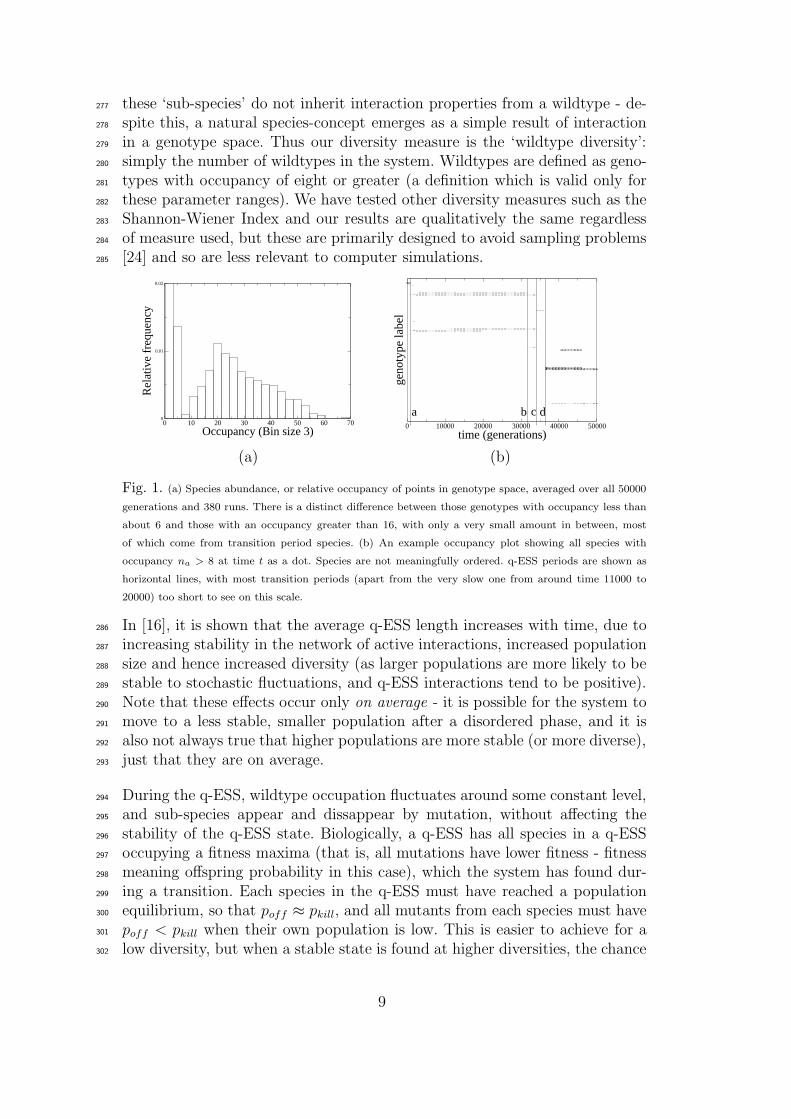
stochastic events (see Figure 1 (a)). As our genotype space is coarse-grained,276

8

these ‘sub-species’ do not inherit interaction properties from a wildtype - de-277

spite this, a natural species-concept emerges as a simple result of interaction278

in a genotype space. Thus our diversity measure is the ‘wildtype diversity’:279

simply the number of wildtypes in the system. Wildtypes are defined as geno-280

types with occupancy of eight or greater (a definition which is valid only for281

these parameter ranges). We have tested other diversity measures such as the282

Shannon-Wiener Index and our results are qualitatively the same regardless283

of measure used, but these are primarily designed to avoid sampling problems284

[24] and so are less relevant to computer simulations.285

0 10 20 30 40 50 60 70

Occupancy (Bin size 3)0

0.01

0.02

Rel

ativ

e fr

eque

ncy

0 10000 20000 30000 40000 50000time (generations)

geno

type

labe

la b c d

(a) (b)

Fig. 1. (a) Species abundance, or relative occupancy of points in genotype space, averaged over all 50000

generations and 380 runs. There is a distinct difference between those genotypes with occupancy less than

about 6 and those with an occupancy greater than 16, with only a very small amount in between, most

of which come from transition period species. (b) An example occupancy plot showing all species with

occupancy na > 8 at time t as a dot. Species are not meaningfully ordered. q-ESS periods are shown as

horizontal lines, with most transition periods (apart from the very slow one from around time 11000 to

20000) too short to see on this scale.

In [16], it is shown that the average q-ESS length increases with time, due to286

increasing stability in the network of active interactions, increased population287

size and hence increased diversity (as larger populations are more likely to be288

stable to stochastic fluctuations, and q-ESS interactions tend to be positive).289

Note that these effects occur only on average - it is possible for the system to290

move to a less stable, smaller population after a disordered phase, and it is291

also not always true that higher populations are more stable (or more diverse),292

just that they are on average.293

During the q-ESS, wildtype occupation fluctuates around some constant level,294

and sub-species appear and dissappear by mutation, without affecting the295

stability of the q-ESS state. Biologically, a q-ESS has all species in a q-ESS296

occupying a fitness maxima (that is, all mutations have lower fitness - fitness297

meaning offspring probability in this case), which the system has found dur-298

ing a transition. Each species in the q-ESS must have reached a population299

equilibrium, so that poff ≈ pkill, and all mutants from each species must have300

poff < pkill when their own population is low. This is easier to achieve for a301

low diversity, but when a stable state is found at higher diversities, the chance302

9

that an invader will destabilise the q-ESS is lower as invaders will be at signif-303

icantly lower fitness on average (due to the increase in the average population304

N from those positive interactions). It is therefore of interest to analyse the305

transition more closely, in order to understand why the q-ESS forms in the306

way it does.307

Transitions appear in many forms, depending on the configuration of the geno-308

type space surrounding the wildtypes. There are two events that can force a309

q-ESS to end:310

• If a genotype with poff > pkill can be reached, then there will be a period311

where the mutant population is still vulnerable to accidental extinction,312

followed by an exponential growth period if the mutant population grows313

large enough. This will usually quickly upset the configuration of the local314

population, leading to transition.315

• If one of the wildtype species had low average population then it can become316

accidentally extinct. In some cases other species will not depend on this317

species and the system enters a similar q-ESS with reduced diversity; in318

other cases, the stability of the q-ESS is upset and a transition occurs.319

Once the system enters a transition, one of the following may happen:320

• The disruption is minor and the system remains stable with a new q-ESS321

configuration. The transition period is not well defined in this case.322

• Wildtype species no longer all have poff = pkill. The populations will change323

in order to regain this relation. It is possible that a species may become324

extinct, leading to stage 2 above.325

• One of the low population mutant species in the system will gain poff > pkill326

and so will enter phase 1 above.327

Clearly, this is an iterative process and can last for a very long time - forever if328

c or pmut are very large, so pushing the system past the ‘error threshold’ [17].329

It is additionally complicated because these processes are all really running330

simultaneously, and responding to each other. What is clear, though, is that331

there is always favoured species in the system, and from simulations we see332

that the number of favoured species does not change significantly from q-333

ESS periods. In [11] it is shown that transition periods retain the distinction334

between (short lived in this case) wildtypes and mutants, resulting in a very335

similar (possibly identical) SAD. Since the transition periods are very short,336

any deviation from the q-ESS SAD is negligible and for an instantaneous337

observation they are indistinguishable (as stochastic noise is high). Transitions338

also provide a way for a species to mutate to a distantly related genotype339

quickly. Because there is a high interaction between all types, and the number340

of types is often quite high, most configurations are not q-ESS. It is therefore341

unlikely that the initial invaders of a q-ESS will be successful in the long342

10

term - they instead will be in turn invaded by a second set of mutants. This343

process continues until a q-ESS is found, and so there is an effective selection344

gradient away from the wildtypes during this time, leading to very large and345

fast changes in genotype acting for short periods of time.346

The species abundances are of log-normal form as observed in many real sys-347

tems [12] provided that the interaction probability Θ is high, as in the cases348

we consider, and the lifetime distribution for species is wide-tailed as in real349

data [11] (following a power-law). More details on the network properties of350

the Tangled Nature model is available from [12], and an in-depth analysis351

of the time dependence of many of the observables such as diversity and to-352

tal population is presented in [16]. Similar work by Zia and Rikvold [25][26]353

deals with a simplification of the non-spatial case. In both models the q-ESS354

wildtypes are characterised as different to transition period wildtypes because355

their mutants do not interact favourably with the q-ESS population, and so356

are suppressed.357

3.2 The Tangled Nature Model on a spatial lattice358

We now introduce a square spatial grid of length X, each containing a TaNa359

model, and allow the lattice-points to interact by migration; migration proba-360

bility refers to the chance of moving to any neighbouring site, chosen randomly361

from the 8 nearest neighbours, and we assume a periodic boundary. Just this362

simple addition to the basic TaNa model gives rise to naturally occurring363

Species-Area Relations, or SARs.364

Unlike the non-spatial version of the model, initial conditions are relevant.365

All possible starting configurations reduce to one of the following two initial366

conditions:367

(1) Individuals are generated with a random genotype and placed on a ran-368

dom lattice point until the total starting population is reached.369

(2) A single lattice point is allowed to evolve as a separate system until a370

q-ESS is formed. This q-ESS is copied to all other lattice points to give371

a quasi-stable, identical initial starting condition at all points.372

Procedure 2 represents the biological case where a small species set is exposed373

to a larger spatial range, and so colonises it. The initial q-ESS used in pro-374

cedure 2 has stability properties that can differ greatly - see Figure 2. It can375

vary in absolute stability (how long it will last for), but spatial duplication376

means that the number of stable q-ESSs that can be found from the initial377

transition is relevant, as this controls how quickly diversity will increase when378

a transition does occur in the system. Procedure 2 therefore introduces a high379

stochastic variation resulting in a (sometimes sharp, sometimes smooth) di-380

11

versity increase after an initial (possibly very long) wait.381

Procedure 1 bears some resemblance to the colonisation of a new area of land382

by many species simultaneously. It results in an initially high diversity as383

different q-ESS states form at all points. This decreases quickly to an similar384

level found from procedure 2. However, after this time, the two procedures are385

equivalent; hence in our analysis we shall consider only initial random seeding,386

i.e. procedure 1, in order to standarize the initial diversity level. We then allow387

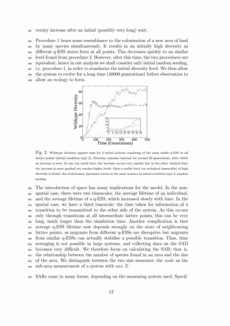
the system to evolve for a long time (40000 generations) before observation to388

allow an ecology to form.389

0 5 10 15 20 25 30 35 4005

101520

0 100 200 300 400 500Time (Generations)

0

20

40

60

80

Wild

type

Div

ersi

ty

Fig. 2. Wildtype diversity against time for 2 initial systems consisting of the same stable q-ESS at all

lattice points (initial condition type 2). Diversity remains constant for around 20 generations, after which

an increase is seen. In one run (solid line), the increase occurs very rapidly but in the other (dashed line)

the increase is more gradual yet reaches higher levels. Once a stable level (on ecological timescales) of high

diversity is found, the evolutionary dynamics occurs in the same manner as initial condition type 2, random

seeding.

The introduction of space has many implications for the model. In the non-390

spatial case, there were two timescales: the average lifetime of an individual,391

and the average lifetime of a q-ESS, which increased slowly with time. In the392

spatial case, we have a third timescale: the time taken for information of a393

transition to be transmitted to the other side of the system. As this occurs394

only through transitions at all intermediate lattice points, this can be very395

long, much longer than the simulation time. Another complication is that396

average q-ESS lifetime now depends strongly on the state of neighbouring397

lattice points, as migrants from different q-ESSs are disruptive but migrants398

from similar q-ESSs can actually stabilise a possible transition. Thus, time399

averaging is not possible in large systems, and collecting data on the SAD400

becomes very difficult. We therefore focus on calculating the SAR: that is,401

the relationship between the number of species found in an area and the size402

of the area. We distinguish between the two size measures: the scale as the403

sub-area measurement of a system with size X.404

SARs come in many forms, depending on the measuring system used. Specif-405

12

ically, quoting [1], there are 3 main properties : “(1) the pattern of quadrats406

or areas sampled (nested, contiguous, noncontiguous, or island); (2) whether407

successively larger areas are constructed in a spatially explicit fashion or not;408

and (3) whether the curve is constructed from single values or mean values”.409

We obtain nested, successive, mean value data. Thus, for all scales, measure-410

ment squares are contained within a larger scales’ measurement square, no411

shapes other than square are considered and we are averaging over all possible412

measuring squares from a specific scale. [1] and [2] discuss the implications for413

this.414

Approximate SAR power-laws are often encountered in real systems at ‘medium’415

scales: that is, for areas that are smaller than the continent/land-mass that416

they are found on, but large enough to obtain a reasonable sample. Good417

examples are plant species in Surrey, UK, ([3], page 9) or bird species in the418

Czech Republic [10]. When looking at other scales different SARs can be ob-419

tained; the distinction between scales is one that varies with environment and420

habitat types, and many functional forms of SAR can be found somewhere.421

A general rule (p277 of [3]) is that inter-provincial relations follow power-law422

SARs with exponent larger than intra-provincially; islands inside a province423

will also have a larger exponent than the whole province itself (thus having424

smaller diversities). A single run in our model corresponds to a single isolated425

province as it is spatially homogenous and self-contained.426

A specific instance of our model will not have any real world equivalent, as427

we have selected genotype space interactions and our initial position in it428

randomly. However, averages over our model should correspond to (large and429

thus self averaging) real systems for which our assumptions are approximately430

valid, as we are effectively averaging over the possible realisations of genotype431

space. Any real world system that does not conform to this average will be432

affected by an effect not modelled here - for example, the geography or resource433

distribution may be an important factor.434

Real systems have z-values between 0.15 and 0.4 depending on the details of435

the system [3]. Figure 3 illustrates real SAR data from Hertfordshire plants436

and shows a sample simulation SAR. Both describe a power-law as are they437

are linear in log-log space, log S = z log A + log α, hence the slope of this line438

(the z-value) is the major controlling factor in how quickly diversity grows439

with area. For example purposes, we have chosen the area of a lattice-point440

arbitrarily as 0.4ha. However the true size of a lattice-point in our model is441

not well defined as the TaNa model implicitly assumes all species are of equal442

spatial extension. Hence we are now concerned only with the scaling relation:443

the form of the SAR being close to a power-law and the value of the exponent444

in that power-law.445

As each run is a separate instance with its own evolutionary history, the diver-446

13

1 10 100 1000 10000

Area (ha for data, arbitrary for simulation)

10

100

Spec

ies

Div

ersi

ty

1 10 100 1000 10000

10

100

Real DataReal data Regression Line (z=0.19)Simulated data

1 10 100Area (Lattice Points)

4

10

50

100

Mea

n W

ildty

pe D

iver

sity

p_move = 0.001p_move = 0.009

Decreasing Pmove

(a) (b)

Fig. 3. (a) SAR Data for Hertfordshire plants taken from [3](Fig 2.2) plotted with simulated data, assuming

1 lattice-point is a 0.4ha plot (pmove = 0.025) evolved for 40000 generations. (b) Simulated, evolved SAR

plotted for varying pmove from 0.001 to 0.009 (in steps of 0.002); the shape and start point remains the

same, with only the exponent changing.

sity and z-value variation between runs is high unless the size is much larger447

than the species range; however, the power-law rule holds for all instances.448

The simulated data in Figure 3 has a slightly reduced tail from the expected449

power-law values, due to the finite area of the simulation. By holding a fixed450

system size (X = 10 is chosen as be the maximum we can simulate with451

sufficient averaging ability) and varying pmove (Figure 4 (a)) we can understand452

these cutoffs more fully.453

0 0.01 0.02P(move)

0

0.2

0.4

0.6

0.8

SAR

z-v

alue

Mean trendStandard errorSpecific run values

100 1000 10000 1e+05Time (Generations)

256

512

Tot

al W

ildty

pe D

iver

sity Wildtype Diversity

Power law fit, z=-0.22

(a) (b)

Fig. 4. (a) z-value calculated from the wildtype diversity evaluated between 40000 and 50000 generations,

showing individual z-values from runs (on a 10x10 lattice). Note the two distinct regions - pmove < 0.01

where species do not spread large enough distances for finite size effects to matter, and pmove > 0.01 where

in some runs, species can span the entire system. (b) log-log plot of diversity as a function of time for a

20x20 system with pmove = 0.005.

Figure 4(a) shows the individual values of z for varying values of pmove together454

with the average. The values are distributed about some mean, which decreases455

approximately linearly with increasing pmove for pmove < 0.01. however, above456

pmove = 0.01 we observe that some of the runs give a near-zero z-value, i.e.457

a constant SAR curve, meaning that species are spanning the system. The458

correlation length of the system has reached the system size and boundary459

affects will irrevocably effect the results. With increasing pmove the average460

14

patch size of each q-ESS increases, and thus the probability of finding a patch461

the size of the system increases. In non-evolutionary models, one can avoid this462

problem by considering migration from a ‘pool’ of constant species makeup463

[27] but in evolving systems the pool must be modelled explicitly.464

Figure 4(b) shows the time dependence of diversity. Although new species465

are produced at all times, and new q-ESS states can be formed, they do not466

seem to do so at a rate that matches diversity loss. The time taken to reach a467

single q-ESS state diverges with area, taking of the order 1012 generations for468

a single q-ESS to be reached for a 20x20 system, or 109 generations for a 10x10469

system. As diversity can increase drastically at any time if a single species can470

destabilise the dominant q-ESS, it is unlikely this would not continue forever.471

Instead, we would effectively be restarting the system with a procedure 2 initial472

condition; however, the stability of this highly evolved q-ESS is much higher473

than a random q-ESS taken from initial conditions, and so the time taken474

to see a restarted system may be very long (as q-ESS lengths are power-law475

distributed, this time has mean infinity - however, it does occur eventually, as476

there is no truly stable state in this model).477

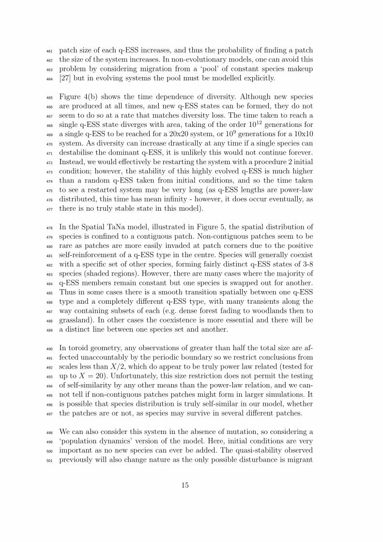
In the Spatial TaNa model, illustrated in Figure 5, the spatial distribution of478

species is confined to a contiguous patch. Non-contiguous patches seem to be479

rare as patches are more easily invaded at patch corners due to the positive480

self-reinforcement of a q-ESS type in the centre. Species will generally coexist481

with a specific set of other species, forming fairly distinct q-ESS states of 3-8482

species (shaded regions). However, there are many cases where the majority of483

q-ESS members remain constant but one species is swapped out for another.484

Thus in some cases there is a smooth transition spatially between one q-ESS485

type and a completely different q-ESS type, with many transients along the486

way containing subsets of each (e.g. dense forest fading to woodlands then to487

grassland). In other cases the coexistence is more essential and there will be488

a distinct line between one species set and another.489

In toroid geometry, any observations of greater than half the total size are af-490

fected unaccountably by the periodic boundary so we restrict conclusions from491

scales less than X/2, which do appear to be truly power law related (tested for492

up to X = 20). Unfortunately, this size restriction does not permit the testing493

of self-similarity by any other means than the power-law relation, and we can-494

not tell if non-contiguous patches patches might form in larger simulations. It495

is possible that species distribution is truly self-similar in our model, whether496

the patches are or not, as species may survive in several different patches.497

We can also consider this system in the absence of mutation, so considering a498

‘population dynamics’ version of the model. Here, initial conditions are very499

important as no new species can ever be added. The quasi-stability observed500

previously will also change nature as the only possible disturbance is migrant501

15

Fig. 5. Spatial distribution of species on a small (5x5) periodic lattice after 50000 generations, with

background shading for each point representing the basic q-ESS members and symbols representing all

genotypes that do not completely fit into a q-ESS category. Some of these genotypes are active in more

than one q-ESS state (e.g. black circle) and others operate in subsets of a specific q-ESS state (e.g. grey

triangle). All species are located in contiguous lattice-points, and it is possible for some patches to span the

entire area.

species. If we for the moment consider a single lattice site with randomly502

chosen species, the behaviour is similar to the usual case with mutation in503

that the number of species condenses down to a small number which are504

mutually stable. As there can be no invasion, the only pressure is accidental505

death. This occurs with very low probability for moderate population numbers506

as the form of poff ensures that there is a restoring pressure to the equilibrium.507

The system will always find a steady state (which, rarely, may have only one508

species in if the species that survived the low population stage happen to all509

have non-mutualistic interactions).510

However, on a spatial lattice things are different. If we choose to evolve a q-511

ESS to copy to all points then clearly the system will contain only this q-ESS512

forever, as there is no source of change. If we start the system with random513

individuals, however, then the initial states found in each lattice point will be514

very different and so migrants may have significant impact. In this case, we515

see a relaxation in diversity of similar form (power law) to the mutation case.516

However, the rate of decay (the exponent for the decrease of diversity with517

time) is smaller compared to the evolving case. A species area relation of the518

same form as in the evolving case is still seen, complete with slight S shape519

form. If we start with an evolved system with a reasonable SAR, and then520

turn off evolution, we see that the decay with time of the diversity decreases521

drastically, as the system almost ‘freezes’ (Figure 6). The SAR form will not522

change drastically, but the exponent will continue to decrease very slowly as523

the number of species, and the number of distinct q-ESS decreases.524

This behaviour shows that it is population dynamics that give the SAR power525

law form, and that our formalism does not permit mutations to spread through526

the system with sufficient speed to offset extinctions. Instead, evolution per-527

mits the generation of ‘better’ q-ESS that can spread through the system528

16

0 2000 4000 6000 8000 10000Time (Generations - linear scale)

114

137

165

198

Mea

n W

ildty

pe D

iver

sity

(lo

g sc

ale)

Mut

atio

ns tu

rned

off

T=5000

Fig. 6. Time dependence of diversity: for the first 5000 generations, mutations are permitted

(pmut = 0.001), and are then stopped (averaged over 20 runs). The system decay rate decreases markedly,

but still follows a power law.

more quickly, accelerating the rate of species loss. However, evolution is re-529

quired to produce diversity in the first place, and allows it to spread very530

quickly throughout the system as seen in Figure 2. In our model, environ-531

mental factors (changing in space and/or evolutionary time) are necessary for532

preventing the collapse of the SAR once it is formed.533

4 Discussion534

Our SAR results bear striking similarity with those of a neutral ‘voting’ model535

of Durrett and Levin [5]. The form of the SAR in both is almost power-law,536

with a slight s-shape produced by boundary effects. They find that the z-value537

decreases with decreasing speciation rate (which is equivalent to immigration538

rate, if new species are introduced from another land mass, for example). In539

our model with interactions and explicit genotype space, we find that z-value540

decreases with increasing migration rate inside the system. Mutation occurs541

at constant speed, so increasing migration rate, e.g. Figure 4(a), decreases542

the relative spread of a new species, instead causing transitions to an already543

existing q-ESS and so reinforcing currently existing species.544

Essentially, internal migration rate reduces the relative effect of mutations,545

and so produces the inverse effect of the immigration rate of new species from546

outside the system (which is equivalent to mutation in a point-mutation rep-547

resentation without consideration of genetics). High mobility (i.e. migration548

and immigration rates) for a family of species mean better mixing and so less549

chance for spatial segregation of species within a single family - the standard550

explanation for why birds generally have lower z-values than land species.551

Conversely, e.g. on islands, it allows species from elsewhere to arrive, so possi-552

bly increasing diversity (as argued in [5]). Which effect dominates will depend553

on the geography in question - i.e. the size of the local groups of individuals,554

17

and the separation between them. A more detailed model is required to probe555

this more fully.556

Magurran and Henderson [28], noted that permanent fish species have log-557

normal SAD whilst transient species have a log-series distribution. Our local558

q-ESS has the same distribution, with a log-normal like distribution for the559

wildtypes and a log-series like for mutants and migrants. For low mutation560

rates and high migration rates, clearly migrants will outnumber local mutants561

and we will observe the exact same distribution near the q-ESS patch borders.562

Here, the distinction between the two types is of fitness - the wildtypes with563

a log-normal like SAD are all equally fit in that they have a reproduction rate564

exactly balancing the death rate; the migrants with a log-series like SAD are565

all less fit and rely on repopulation from an external pool.566

The Tangled Nature model on a spatial lattice reproduces many of the ob-567

served features in real systems without making any a-priori assumptions about568

the existence of species. Instead, species and their spatial distributions are al-569

lowed to form naturally by co-evolution from simple rules applied only to570

individuals. Unfortunately, the model is currently too computer intensive to571

allow simulation of the very large scales (and higher migration rates) expected572

in real systems. However, a near power law is clearly produced as a simple573

result of species forming patches of many sizes, themselves the product of574

diffusive dispersion with reproduction and mutation when local interaction is575

permitted. Mutation is necessary to give ‘raw material’ for new species to be576

formed.577

Co-evolutionary forces are sufficient to allow (co-evolutionary) habitat differ-578

entiation (as shown in the co-habitation of competing E.coli strains in [29]),579

and the number of different habitats increases with area as a power-law. Thus580

power-law SARs are observed, as the number of habitats can drive the diver-581

sity increase with area [3], and these persist over long timescales and in the582

absence of geographical differences. The evolutionary history therefore relates583

to the production, and z-value, of power-law like SARs and may be important584

in many cases [3].585

The habitat differentiation produced by co-evolution allows species to be lo-586

cally equivalent whilst interacting strongly, and maintains differences in off-587

spring probabilities when removed from its favoured habitat. Thus we find588

equivalence whenever individuals have had time to adapt to the homoge-589

neous killing probability, which corresponds to a situation where individuals590

die mainly due to some more our less species independent stochastic killing591

mechanism. An example of such a system might be ‘climax’ stage of forest592

succession [30][31], where species makeup is approximately constant (over a593

sufficiently large area and time average) and the ratio of births to deaths are594

close to unity for all species. Species measured in the field that were found595

18

to be non-equivalent [7] may be considered in the context of Tangled Nature596

to be transitionary, or may simply be out of the habitat they were originally597

adapted to - the equivalence predicted in our system is very local, but can be598

formed over distances by the correct migration composition of species.599

Individuals from species not found locally are generally poorly adapted to600

the local environment and go quickly extinct. Rarely, however, species with601

poff > pkill can invade and their increased chance of survival over the general602

population allows the species to flourish initially - providing a method for fast603

speciation from an initial mutant. In addition, during transitions, intermediate604

genotypes are successful which may be replaced by other genotypes before a605

q-ESS is established, overcoming the ‘fitness barrier’ to distant genotypes,606

with all intermediates occupying fitness maxima. Thus, speciation can occur607

quickly, and to species distantly related. This contrasts the ‘fitness landscape’608

viewpoint (For a review, see e.g. [32]), in which speciation requires passing609

through a fitness minima. It also solves a problem seen in neutral theories,610

which require external pressure such as allopatric speciation (i.e. isolating a611

whole community for mutation by “random fission” [33][34], instead of using612

the traditional point mutation used here and in much of the literature) if613

realistically fast speciation and extinctions are to occur [7].614

We have identified the stability of species, fast extinctions and separation in615

genotype space as the main differences between our interacting model and616

neutral models. The wildtypes in our system are locally equivalent, and it617

is the patches of these wildtypes that are producing the power-law SARs618

observed. Wildtypes are thus equivalent most of the time but not when found619

outside their own habitat, where they suffer a reproductive disadvantage. This620

is consistent with the non-neutrality observed in nature and may explain why621

neutral dynamics do so well at predicting SARs and SADs. The non-neutrality622

is only important during transitions (which, in the spatial model are usually623

local events), but the number and distribution of species does not change, only624

the specific type of species. These effects cannot be observed in instantaneous625

measures, or in time averages.626

The spatial Tangled Nature model provides a simple general framework con-627

taining the basic properties of diffusive dispersion, reproduction and mutation628

on the level of individuals, it allows taxonomic structures to emerge and pro-629

duces a large number of observed macroscopic ecological phenomenon - species630

abundance, long-lived species, fast extinctions, power-law lifetimes, intermit-631

tent dynamics, and, as demonstrated in the present paper, species-area rela-632

tions.633

19

Acknowledgements634

We thank Andy Thomas and Gunnar Pruessner for providing assistance with processing the model and635

setting up the BSD cluster, speeding computation enormously. We also thank the Engineering and Physical636

Sciences Research Council (EPSRC) for Daniel Lawson’s PhD studentship.637

References638

[1] Samuel M. Scheiner. Six types of species-area curves. Glob. Ecol. & Biogeog.,639

12:441–447, 2003.640

[2] Even Tjørve. Shapes and functions of species-area curves: a review of possible641

models. J. of Biogeog., 30:827–835, 2003.642

[3] Michael L. Rosenzweig. Species diversity in space and time. Cambridge643

University Press, The Edinburgh Building, Cambridge CB2 2RU, 1995.644

[4] Stephen Hubbell. The Unified Neutral Theory of Biodiversity and Biogeography.645

Princeton University Press, 41 William Street, Princeton, New Jersey 08540,646

2001.647

[5] Rick Durrett and Simon Levin. Spatial models for species-area curves. J. theor.648

Biol., 179:119–127, 1996.649

[6] Igor Volkov, Jayanth R. Banavar, Stephen P. Hubbell, and Amos Marita.650

Neutral theory and relative species abundance in ecology. Nature, 424:1035–651

1037, 2003.652

[7] J. Chave. Neutral theory and community ecology. Ecol. Let., 7:241–253, 2004.653

[8] Ricard V. Sole, David Alonso, and Alan McKane. Self-organised instability in654

complex ecosystems. Phil. Trans. R. Soc. Lond. B, 357:667–681, 2002.655

[9] John Harte, Tim Blackburn, and Annette Ostling. Self-similarity and the656

relationship between abundance and range size. Am. Nat., 157:374–386, 2001.657

[10] Arnost L. Sizling and David Storch. Power-law species-area relationships and658

self-similar species distributions within finite areas. Ecology Let., 7:60–68, 2004.659

[11] Kim Christensen, Simone A. di Collobiano, Matt Hall, and Henrik J. Jensen.660

Tangled nature: A model of evolutionary ecology. J. Theor. Biol., 216:73–84,661

2002.662

[12] Paul Anderson and Henrik Jeldtoft Jensen. Network properties, species663

abundance and evolution in a model of evolutionary ecology. Journal of664

Theoretical Biology, 232:551–558, 2005.665

[13] Daniel Lawson, Henrik Jeldtoft Jensen, and Kunihiko Kaneko. Diversity as a666

product of interspecial interactions. arXiv:q-bio.PE, (0505019), 2005.667

[14] Edward F. Connor and Earl D. McCoy. The statistics and biology of the species-668

area relationship. Am. Nat., 113:791–833, 1979.669

[15] Andreas Rechtsteiner and Mark A. Bebau. A generic neutral model for670

measuring excess evolutionary activity of genotypes. GECCO-99: Proceedings671

of the Genetic and Evolutionary Computation Conference, July 13-17, 1999,672

Orlando, Florida, pages 1366–1373, 1999.673

[16] Matt Hall, Kim Christensen, Simone A. di Collobiano, and Henrik Jeldtoft674

Jensen. Time-dependent extinction rate and species abundance in a tangled-675

nature model of biological evolution. Phys. Rev. E, 66, 2002.676

20

[17] Simone Avogadro di Collobiano, Kim Christensen, and Henrik Jeldtoft Jensen.677

The tangled nature model as an evolving quasi-species model. J. Phys A,678

36:883–891, 2003.679

[18] Dietrich Stauffer, Ambarish Kunwar, and Denashish Chowdhury. Evolutionary680

ecology in silico: evolving food webs, migrating population and speciation.681

Physica A, pages 202–215, 2005.682

[19] Sergey Gavrilets. Fitness Landscapes and the Origin of Species. Princeton683

University Press, 41 William Street, Princeton, New Jersey 08540, 2004.684

[20] Simon Laird and Henrik Jeldtoft Jensen. The tangled nature model with685

inheritance and constraint: Evolutionary ecology constricted by a conserved686

resource. Unpublished work, 2005.687

[21] Egbert H. van Nes and Marten Scheffer. Large species shifts triggered by small688

forces. Am. Nat., 164:255–266, 2004.689

[22] Kei Tokita and Ayumu Yasutomi. Emergence of a complex and stable network690

in a model ecosystem with extinction and mutation. Theor. Pop. Biol., pages691

131–146, 2003.692

[23] J. Maynard Smith. Evolution and the theory of games. Cambridge University693

Press, The Edinburgh Building, Cambridge CB2 2RU, 1982.694

[24] Anne E. Magurran. Measuring Biological Diversity. Blackwell Science Limited,695

108 Cowley Road, Oxford, OX4 1JF, 2004.696

[25] Per Arne Rikvold and R. K. P. Zia. Punctuated equilibria and 1/f noise in a697

biological coevolution model with individual-based dynamics. Phys. Rev. E, 68,698

2003.699

[26] R K P Zia and Per Arne Rikvold. Fluctuations and correlations in an individual-700

based model of evolution. J. Phys. A, 37:5135–5155, 2004.701

[27] R. H. MacArthur and E. O. Wilson. The Theory of Island Biogeography.702

Princeton University Press, Princeton, NJ, USA, 1967.703

[28] Anne E. Magurran and Peter A. Henderson. Explaining the excess of rare704

species in natural species abundance distributions. Nature, pages 714–716, 2003.705

[29] Akiko Kashiwagi, Wataru Noumachi, Masato Katsuno, Mohammad T. Alam,706

Itaru Urabe, and Tetsuya Yomo. Plasticity of fitness and diversification process707

during an experimental molecular evolution. J. Molec. Evol., 52:502–509, 2001.708

[30] N. A. Cambell. Biology. Benjamin/Cummings Publ. Co., 2725 Sand Hill Road,709

Menlo Park, California 94025, 1996.710

[31] Erik R. Pianka. Evolutionary Ecology. Addison Wesley Educational Publishers,711

1301 Sansome St, San Francisco, CA 94111, 2000.712

[32] Barbara Drossel. Biological evolution and statistical physics. Cond. Mat., 2001.713

[33] Stephen P. Hubbell. Modes of speciation and the lifespans of species under714

neutrality: a response to the comment of robert e. ricklefs. OIKOS, 100:193–715

199, 2003.716

[34] Robert E. Ricklefs. A comment on hubbell’s zero-sum ecological drift model.717

OIKOS, 100:185–192, 2003.718

[35] Drew W. Purves and Stephen W Pacala. Ecological drift in niche-structured719

communities: neutral pattern does not imply neutral process. In D. Burslem,720

M. Pinard, and S. Hartley, editors, Biotic Interactions in the Tropics - Their721

Role in the Maintenance of Species Diversity. Cambridge University Press, The722

Edinburgh Building, Shaftesbury Road, Cambridge, CB2 2RU, 2005.723

21