arX

iv:1

208.

0434

v1 [

mat

h.M

G]

2 A

ug 2

012

The space of spaces:

curvature bounds and gradient flows on the space of

metric measure spaces

Karl-Theodor Sturm

Abstract

Equipped with the L2-distortion distance ∆∆, the space X of all metric measure spaces (X, d,m) isproven to have nonnegative curvature in the sense of Alexandrov. Geodesics and tangent spaces arecharacterized in detail. Moreover, classes of semiconvex functionals and their gradient flows on X arepresented.

Introduction and Main Results at a Glance

I. The basic object of this paper is the space X of isomorphism classes of metric measure spaces. A metricmeasure space is a triple (X, d,m) consisting of a space X , a complete separable metric d on X and aBorel probability measure on it (more precisely, a probability measure on the Borel σ-field induced by

the metric d on X). We will always require that its L2-size(∫

X

∫Xd2(x, y)dm(x)dm(y)

)1/2is finite. Two

metric measure spaces with full supports are isomorphic if there exists a measure preserving isometrybetween them.We will consider X as a metric space equipped with the so-called L2-distortion distance ∆∆ = ∆∆2 to bepresented below. One of our main results is that

the metric space (X,∆∆) has nonnegative curvature in the sense of Alexandrov.

Both the triangle comparison and the quadruple comparison will be verified.

II. The Lp-distortion distance between two metric measure spaces (X0, d0,m0) and (X1, d1,m1) is definedfor p ∈ [1,∞) as

∆∆p

((X0, d0,m0), (X1, d1,m1)

)

= infm∈Cpl(m0,m1)

(∫

X0×X1

∫

X0×X1

∣∣∣d0(x0, y0)− d1(x1, y1)∣∣∣p

dm(x0, x1)dm(y0, y1)

)1/p

where the infimum is taken over all couplings of m0 and m1, i.e. over all probability measures m onX0×X1

with prescribed marginals (π0)∗m = m0 and (π1)∗m = m1. There always exists an optimal coupling forwhich the infimum is attained. Convergence w.r.t. the Lp-distortion distance can be characterized asconvergence w.r.t. the L0-distortion distance together with convergence of the Lp-size. The L0-distortiondistance induces the same topology as the L0-transportation distance (also known as Prohorov-Gromov

1

metric) which in turn is equivalent to Gromov’s box metric λ.One of our fundamental results – with far reaching applications – is a complete, explicit characterizationof ∆∆p-geodesics in X:

For each optimal coupling m, the family of metric measure spaces(X0 ×X1, (1− t) d0 + t d1, m

)for t ∈ (0, 1)

defines a geodesic in X connecting (X0, d0,m0) and (X1, d1,m1).

If p ∈ (1,∞), then each geodesic in X is of this form.

For each metric measure space (X, d,m), a geodesic ray through it is given by (X, t · d,m) for t ≥ 0. Itsinitial point is the one-point space δ (= the equivalence class of metric measure spaces whose supportsconsist of one point). In the particular case p = 2, (X,∆∆) is a cone with apex δ over its unit sphere.

III. X is quite a huge space: it contains all Riemannian manifolds, GH-limits of Riemannian manifolds(cf. [CC97, CC00a, CC00b]), Finsler spaces (cf. [She01], [OS09]), finite dimensional Alexandrov spaces(cf. [BGP92], [OS94]) , groups (cf. [Woe00]), graphs (cf. [Del99]), fractals (cf. [Kig01]) as well as manyinfinite dimensional spaces (cf. [BSC05]) – provided the respective spaces, manifolds, graphs etc. havefinite volume (which then is assumed to be normalized). In particular, it contains all metric measurespaces with generalized lower bounds for the Ricci curvature in the sense of Lott-Sturm-Villani [Stu06],[LV09].

However, X is not complete w.r.t. ∆∆. Fortunately, each element in its completion X again can berepresented as a triple (X, d,m) – more precisely, as an equivalence class (‘homomorphism class’) of suchtriples – where X is a Polish space, m a Borel probability measure on X and d a symmetric, squareintegrable Borel function on X ×X which satisfies the triangle inequality almost everywhere. That is,

the completion of X is the space X of pseudo metric measure spaces.

The ‘space of spaces’ (X,∆∆) is a complete, geodesic space of nonnegative curvature (infinite dimensionalAlexandrov space) and as such allows for a variety of geometric concepts including space of geodesicdirections, tangent cones, exponential maps, gradients of semiconvex functions, and (downward) gradientflows.

IV. A deeper insight into the tangent structure of X is obtained by regarding X as a closed convex subsetof an ambient space Y which consists of equivalence classes of triples (X, d,m) – called gauged measurespaces – with X being Polish, d a symmetric L2-function on X2 (no longer required to satisfy the triangleinequality) and m a Borel probability measure on X . It turns out that

the metric space (Y,∆∆) is isometric to the quotient space L2s(I

2,L2)/ Inv(I,L)

where L2s(I

2,L2) denotes the space of symmetric L2-functions on the unit square and Inv(I,L) denotesthe space of measure preserving transformations of the unit interval I = [0, 1]. Being isometric to thequotient of a Hilbert space under the action of a semigroup (acting isometrically via pull back), it comesas no surprise that (Y,∆∆) is again a complete, geodesic metric space of nonnegative curvature.

A more detailed analysis of the tangent structure allows to regard Y as an infinite dimensionalRiemannian orbifold. In fact, one always may choose a homomorphic representative (X, d,m) withoutatoms. Then

the tangent space of the triple (X, d,m) is given by

T(X,d,m)Y = L2s(X

2,m2)/ Sym(X, d,m)

where Sym(X, d,m) denotes the symmetry group (or isotropy group) of (X, d,m).

2

In particular, if the given space (X, d,m) has no non-trivial symmetries then its tangent space is Hilbertianand for f ∈ L2

s(X2,m2)

Exp(X,d,m)(f) = (X, d+ f,m).

These results are very much in the spirit of Otto’s Riemannian calculus [Ott01] on the L2-Wassersteinspace P2(R

n) which also leads to lower bounds on the sectional curvature (cf. [Lot08]) and quite detailedstructural assertions on the tangent space (cf. [AGS05]). The latter, however, is essentially limitedto ‘regular’ points (i.e. absolutely continuous measures) whereas the above results also provide preciseassertions on the tangent structure for ‘non-regular’ points (i.e. spaces with non-trivial symmetries).

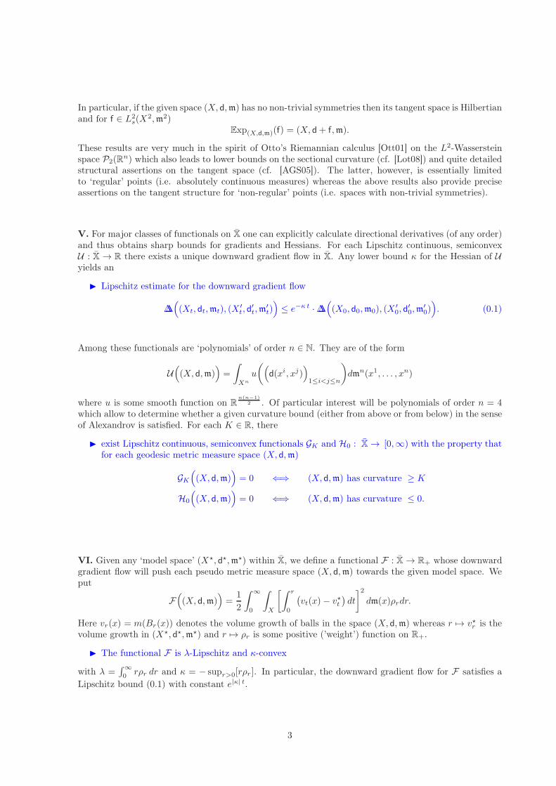
V. For major classes of functionals on X one can explicitly calculate directional derivatives (of any order)and thus obtains sharp bounds for gradients and Hessians. For each Lipschitz continuous, semiconvexU : X → R there exists a unique downward gradient flow in X. Any lower bound κ for the Hessian of Uyields an

Lipschitz estimate for the downward gradient flow

∆∆((Xt, dt,mt), (X

′t, d′t,m′t))≤ e−κ t ·∆∆

((X0, d0,m0), (X

′0, d′0,m

′0)). (0.1)

Among these functionals are ‘polynomials’ of order n ∈ N. They are of the form

U((X, d,m)

)=

∫

Xn

u

((d(xi, xj)

)1≤i<j≤n

)dmn(x1, . . . , xn)

where u is some smooth function on Rn(n−1)

2 . Of particular interest will be polynomials of order n = 4which allow to determine whether a given curvature bound (either from above or from below) in the senseof Alexandrov is satisfied. For each K ∈ R, there

exist Lipschitz continuous, semiconvex functionals GK and H0 : X → [0,∞) with the property thatfor each geodesic metric measure space (X, d,m)

GK

((X, d,m)

)= 0 ⇐⇒ (X, d,m) has curvature ≥ K

H0

((X, d,m)

)= 0 ⇐⇒ (X, d,m) has curvature ≤ 0.

VI. Given any ‘model space’ (X⋆, d⋆,m⋆) within X, we define a functional F : X → R+ whose downwardgradient flow will push each pseudo metric measure space (X, d,m) towards the given model space. Weput

F((X, d,m)

)=

1

2

∫ ∞

0

∫

X

[∫ r

0

(vt(x)− v⋆t

)dt

]2dm(x)ρrdr.

Here vr(x) = m(Br(x)) denotes the volume growth of balls in the space (X, d,m) whereas r 7→ v⋆r is thevolume growth in (X⋆, d⋆,m⋆) and r 7→ ρr is some positive (’weight’) function on R+.

The functional F is λ-Lipschitz and κ-convex

with λ =∫∞0rρr dr and κ = − supr>0[rρr ]. In particular, the downward gradient flow for F satisfies a

Lipschitz bound (0.1) with constant e|κ| t.

3

The functional F will vanish if and only if

vr(x) = v⋆r for every r ≥ 0 and m-a.e. x ∈ X.

If X is a Riemannian manifold and v⋆ denotes the volume growth of the Riemannian model space Mn,κ

for n ≤ 3 and κ > 0 then the previous property implies that X is the model space Mn,κ.

The gradient of −F at the point (X, d,m) is explicitly given as the function f ∈ L2s(X

2,m2) with

f(x, y) =

∫ ∞

0

(vr(x) + vr(y)

2− v⋆r

)ρ(r ∨ d(x, y)

)dr

where ρ(a) =∫∞aρrdr.

The infinitesimal evolution of (X, d,m) under the downward gradient flow for F on X is given by (X, dt,m)with

dt(x, y) = d(x, y) + tf(x, y) +O(t2)

and f as above. That is, d(x, y) will be enlarged if – in average w.r.t. the radius r – the volume of ballsBr(x) and Br(y) in X is too large (compared with the volume v⋆r of balls in the model space), and d(x, y)will be reduced if the volume of balls is too small.

VII. In a broader sense, the downward gradient flow for F is related to Ricci flow. Indeed, on the spaceof Riemannian manifolds, the functionals F (ǫ) for a suitable sequence of weight functions ρ(ǫ) (convergingto δ0) will converge to

1

2

∫

X

(s(x) − s⋆)2dm(x),

a modification of the Einstein-Hilbert functional which plays a key role in Perelman’s program [Per02],cf. [MT07], [KL08].

Note that Ricci flow does not depend continuously on the initial data, in particular, no Lipschitzestimate of the form (0.1) will hold. Also note that no “regularizing” gradient flow is known which respectslower curvature bounds in the sense of Alexandrov (Petrunin [Pet07b]: “Please deform an Alexandrov’sspace”). Similarly, no “regularizing” gradient flow is known which respects lower Ricci bounds in the senseof Lott-Sturm-Villani [Stu06], [LV09].

This paper provides a comprehensive and detailed picture of the geometry in the space X of all pseudometric measure spaces. Nevertheless, many challenging questions remain open, e.g.

• For which pairs of Riemannian manifolds does the connecting ∆∆-geodesic stay within the space ofRiemannian manifolds?

• For which functionals U : X → R does the gradient flow stay within the space of Riemannianmanifolds (if started there)?

Acknowledgement. The author would like to thank Fabio Cavalletti, Matthias Erbar, Martin Huesmann,Christian Ketterer and in particular Nora Loose for carefully reading early drafts of this paper andfor many valuable comments. He also gratefully acknowledges stimulating discussions on topics of thispaper with Nicola Gigli, Jan Maas, Shin-ichi Ohta, Takashi Shioya, Asuka Takatsu and Anatoly Vershikin Bonn as well as during conferences in Pisa, Oberwolfach and Sankt Petersburg (May, June 2012).In particular, he is greatly indebted to Andrea Mondino for enlightening discussions on criteria forRiemannian manifolds to be balanced (Theorem, 8.13).

4

Contents

1 The Metric Space (Xp,∆∆p) 61.1 Metric Measure Spaces and Couplings . . . . . . . . . . . . . . . . . . . . . . . . . . . . . 61.2 The Lp-Distortion Distance . . . . . . . . . . . . . . . . . . . . . . . . . . . . . . . . . . . 81.3 Isomorphism Classes of MM-Spaces . . . . . . . . . . . . . . . . . . . . . . . . . . . . . . . 9

2 The Topology of (Xp,∆∆p) 132.1 Lp-Distortion Distance vs. L0-Distortion Distance . . . . . . . . . . . . . . . . . . . . . . 132.2 Lp-Distortion Distance vs. Lp-Transportation Distance . . . . . . . . . . . . . . . . . . . . 142.3 L0-Distortion Distance vs. L0-Transportation Distance and Gromov’s Box Distance . . . 17

3 Geodesics in (Xp,∆∆p) 19

4 Cone Structure and Curvature Bounds for (X,∆∆) 244.1 Cone Structure . . . . . . . . . . . . . . . . . . . . . . . . . . . . . . . . . . . . . . . . . . 244.2 Curvature Bounds . . . . . . . . . . . . . . . . . . . . . . . . . . . . . . . . . . . . . . . . 264.3 Space of Directions, Tangent Cone, and Gradients on X . . . . . . . . . . . . . . . . . . . 284.4 Gradient Flows on X . . . . . . . . . . . . . . . . . . . . . . . . . . . . . . . . . . . . . . . 29

5 The Space Y of Gauged Measure Spaces 305.1 Gauged Measure Spaces . . . . . . . . . . . . . . . . . . . . . . . . . . . . . . . . . . . . . 305.2 Equivalence Classes in L2

s(I2,L2) . . . . . . . . . . . . . . . . . . . . . . . . . . . . . . . . 34

5.3 Pseudo Metric Measure Spaces . . . . . . . . . . . . . . . . . . . . . . . . . . . . . . . . . 365.4 The n-Point Spaces . . . . . . . . . . . . . . . . . . . . . . . . . . . . . . . . . . . . . . . . 40

6 The Space Y as a Riemannian Orbifold 456.1 The Symmetry Group . . . . . . . . . . . . . . . . . . . . . . . . . . . . . . . . . . . . . . 456.2 Geodesic Hinges . . . . . . . . . . . . . . . . . . . . . . . . . . . . . . . . . . . . . . . . . 466.3 Tangent Spaces and Tangent Cones . . . . . . . . . . . . . . . . . . . . . . . . . . . . . . . 486.4 Tangent Spaces – A Comprehensive Alternative Approach . . . . . . . . . . . . . . . . . . 516.5 Ambient Gradients . . . . . . . . . . . . . . . . . . . . . . . . . . . . . . . . . . . . . . . . 52

7 Semiconvex Functions on Y and their Gradients 537.1 Polynomials on Y and their Derivatives . . . . . . . . . . . . . . . . . . . . . . . . . . . . 537.2 Nested Polynomials . . . . . . . . . . . . . . . . . . . . . . . . . . . . . . . . . . . . . . . . 567.3 The G-Functionals . . . . . . . . . . . . . . . . . . . . . . . . . . . . . . . . . . . . . . . . 597.4 The H-Functionals . . . . . . . . . . . . . . . . . . . . . . . . . . . . . . . . . . . . . . . . 61

8 The F-Functional 628.1 Balanced spaces . . . . . . . . . . . . . . . . . . . . . . . . . . . . . . . . . . . . . . . . . . 628.2 The F -Functional and its Gradient Flow . . . . . . . . . . . . . . . . . . . . . . . . . . . . 67

5

1 The Metric Space (Xp,∆∆p)

1.1 Metric Measure Spaces and Couplings

Throughout this paper, a metric measure space (briefly: mm-space) will always be a triple (X, d,m)where

• (X, d) is a complete separable metric space,

• m is a Borel probability measure on X .

The latter means that m is a measure on B(X) – the Borel σ-field associated with the Polish topologyon X induced by the metric d – with normalized total mass m(X) = 1. In the literature, metric measurespaces are also called metric triples.

The support supp(X, d,m) of such a metric measure space – or simply the support supp(m) of themeasure m – is the smallest closed set X0 ⊂ X such that m(X \ X0) = 0. Occasionally, it will also bedenoted by X. We say that (X, d,m) has full support if supp(X, d,m) = X . This, however, will notbe required in general. The diameter or L∞-size of a metric measure space (X, d,m) is defined as thediameter of its support:

diam(X, d,m) = supd(x, y) : x, y ∈ supp(X, d,m)

.

For any p ∈ [1,∞), the Lp-size of (X, d,m) is defined as

sizep(X, d,m) :=

(∫

X

∫

X

dp(x, y)dm(x)dm(y)

)1/p

.

Obviously, sizep(X, d,m) ≤ sizeq(X, d,m) ≤ diam(X, d,m) for all 1 ≤ p ≤ q ≤ ∞.Given two mm-spaces (X0, d0,m0) and (X1, d1,m1) and a map ψ : X0 → X1, we define

• the pull back of the metric d1 through ψ as the pseudo metric ψ∗d1 on X0 given by

(ψ∗d1)(x0, y0) = d1(ψ(x0), ψ(y0))(∀x0, y0 ∈ X0

);

• the push forward of the probability measure m0 through ψ – provided ψ is Borel measurable – asthe probability measure ψ∗m0 on (X1,B(X1)) given by

(ψ∗m0)(A1) = m0

(ψ−1(A1)

)= m0

(x0 ∈ X0 : ψ(x0) ∈ A1

) (∀A1 ∈ B(X1)

).

Definition 1.1. Given two mm-spaces (X0, d0,m0) and (X1, d1,m1), any probability measure m on theproduct space X0 ×X1 (equipped with the product topology and product σ-field) satisfying

(π0)∗m = m0, (π1)∗m = m1 (1.1)

is called coupling of the measures m0 and m1. The measures m0 and m1 in turn will be called marginalsof m.

Here π0 and π1 denote the projections from X0 × X1 to X0 and X1, resp. Condition (1.1) can berestated as:

m(A0 ×X1) = m0(A0), m(X0 ×A1) = m1(A1)

for all A0 ∈ B(X0), A1 ∈ B(X1). The set of all couplings of m0 and m1 will be denoted by Cpl(m0,m1).The set Cpl(m0,m1) is non-empty: it always contains the product coupling m = m0 ⊗ m1 (being

uniquely defined by the requirement m(A0 × A1) = m0(A0) · m1(A1) for all A0 ∈ B(X0), A1 ∈ B(X1)).If one of the measures m0 and m1 is a Dirac then the product coupling is indeed the only coupling:Cpl(δx0 ,m1) = δx0 ⊗m1.Lemma 1.2. Given m0 and m1, the set of couplings Cpl(m0,m1) is a non-empty compact subset ofP(X0 ×X1), the set of probability measures on X0 ×X1 equipped with the weak topology.

6

Proof. Obviously, Cpl(m0,m1) is a closed subset within P(X0×X1). (The projection maps are continuousfunctions.) The relative compactness (‘tightness’) follows from a simple application of Prohorov’s theorem,see [Vil09], Lemma 4.4.

For each measurable map ψ : X0 → X1 with ψ∗m0 = m1, a coupling of m0 and m1 is given by

m = (Id, ψ)∗m0.

In the particular case X0 = X1, m0 = m1, the choice ψ = Id leads to the diagonal coupling

dm(x, y) = dδx(y) dm0(x).

More generally, for each mm-space (X, d,m) and measurable maps ψ0 : X → X0, ψ1 : X → X1 with(ψ0)∗m = m0, (ψ1)∗m = m1, a coupling of m0 and m1 is given by

m = (ψ0, ψ1)∗m.

Indeed, any coupling is of this form – and without restriction one may choose (X, d,m) to be the unitinterval X = [0, 1] equipped with the standard distance d(x, y) = |x− y| and the 1-dimensional Lebesguemeasure m = L1 on [0, 1], cf. Lemma 1.15.

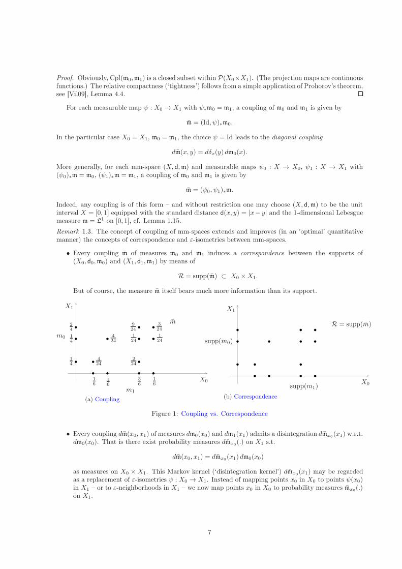
Remark 1.3. The concept of coupling of mm-spaces extends and improves (in an ’optimal’ quantitativemanner) the concepts of correspondence and ε-isometries between mm-spaces.

• Every coupling m of measures m0 and m1 induces a correspondence between the supports of(X0, d0,m0) and (X1, d1,m1) by means of

R = supp(m) ⊂ X0 ×X1.

But of course, the measure m itself bears much more information than its support.

24

14

14

36

16

16

16

424

424

124

124

224

924

324

X0

X1

m

m0

m1

(a) Coupling

X0

X1

R = supp(m)

supp(m0)

supp(m1)

(b) Correspondence

Figure 1: Coupling vs. Correspondence

• Every coupling dm(x0, x1) of measures dm0(x0) and dm1(x1) admits a disintegration dmx0(x1) w.r.t.dm0(x0). That is there exist probability measures dmx0(.) on X1 s.t.

dm(x0, x1) = dmx0(x1) dm0(x0)

as measures on X0 ×X1. This Markov kernel (‘disintegration kernel’) dmx0(x1) may be regardedas a replacement of ε-isometries ψ : X0 → X1. Instead of mapping points x0 in X0 to points ψ(x0)in X1 – or to ε-neighborhoods in X1 – we now map points x0 in X0 to probability measures mx0(.)on X1.

7

Lemma 1.4 (Gluing lemma). Let X0, X1, . . . , Xk be Polish spaces and m0,m1, . . . ,mk probability mea-sures, defined on the respective σ-fields. Then for every choice of couplings µi ∈ Cpl(mi−1,mi), i =1, . . . , k, there exists a unique probability measure µ ∈ P(X0 ×X1 × . . .×Xk) s.t.

(πi−1, πi)∗µ = µi (∀i = 1, . . . , k). (1.2)

µ is called gluing of the couplings µ1, . . . , µk and denoted by

µ = µ1 ⊠ . . .⊠ µk.

In particular, µ has marginals m0,m1, . . . ,mk. That is, (πi)∗µ = mi for all i = 0, 1, . . . , k. Note,however, that the latter (in contrast to (1.2)) does not determine µ uniquely.

Proof. The proof in the case k = 2 is well-known, see e.g. [Dud02], proof of Lemma 11.8.3, [Vil03], Lemma7.6. For convenience of the reader, let us briefly recall the construction: disintegration of dµ1(x0, x1) w.r.t.dm1(x1) yields a Markov kernel dpx1(x0) such that

dµ1(x0, x1) = dpx1(x0)dm1(x1).

Similarly, disintegration of dµ2(x1, x2) w.r.t. dm1(x1) leads to a kernel dqx1(x2). In terms of these kernelsthe probability measure µ = µ1 ⊠ µ2 on X0 ×X1 ×X2 is defined as

dµ(x0, x1, x2) = dpx1(x0)dqx1(x2)dm1(x1).

The solution for general k is constructed iteratively. Assume that µ(i) := µ1 ⊠ . . . ⊠ µi is alreadyconstructed. By definition/construction it is a coupling of µ(i−1) and mi whereas µi+1 is a coupling ofmi and mi+1. The previous step thus allows to construct the gluing of µ(i) and µi+1 which is the desiredµ(i+1) = µ(i) ⊠ µi+1.

Lemma 1.5. Let X0 and Xk, k ∈ N, be Polish spaces and m0 and mk, k ∈ N, probability measures,defined on the respective σ-fields. Then for every choice of couplings µk ∈ Cpl(m0,mk), k ∈ N, thereexists a probability measure µ ∈ P

(∏∞k=0Xk

)s.t.

(π0, πk)∗µ = µk (∀k ∈ N). (1.3)

Proof. Let µk ∈ Cpl(m0,mk) for k ∈ N be given and define for each n ∈ N a probability measure µ(n) onX = X0 ×X1 × . . . Xn by

dµ(n)(x0, x1, x2, . . . , xn) = dµ1,x0(x1) dµ2,x0(x2) . . . dµn,x0(xn) dm0(x0)

where dµk,x0(xk) denotes the disintegration of dµk(x0, xk) w.r.t. dm0(x0). The projective limit of theseprobability measures µ(n) as n→ ∞ is the requested µ.

1.2 The Lp-Distortion Distance

Definition 1.6. For any p ∈ [1,∞), the Lp-distortion distance between two metric measure spaces(X0, d0,m0) and (X1, d1,m1) is defined as

∆∆p((X0, d0,m0), (X1, d1,m1))

= inf

(∫

X0×X1

∫

X0×X1

|d0(x0, y0)− d1(x1, y1)|p dm(x0, x1)dm(y0, y1)

)1/p

: m ∈ Cpl(m0,m1)

.

Similarly, the L∞-distortion distance is defined as

∆∆∞((X0, d0,m0), (X1, d1,m1))

= inf

sup

|d0(x0, y0)− d1(x1, y1)| : (x0, x1), (y0, y1) ∈ supp(m)

: m ∈ Cpl(m0,m1)

.

8

Lemma 1.7. For each p ∈ [1,∞] and each pair of metric measure spaces (X0, d0,m0) and (X1, d1,m1),the infimum in the definition of ∆∆p((X0, d0,m0), (X1, d1,m1)) will be attained. That is, there exists ameasure m ∈ Cpl(m0,m1) such that

∆∆p((X0, d0,m0), (X1, d1,m1)) =

(∫

X0×X1

∫

X0×X1

|d0(x0, y0)− d1(x1, y1)|p dm(x0, x1)dm(y0, y1)

)1/p

(1.4)in the case p <∞ and

∆∆∞((X0, d0,m0), (X1, d1,m1)) = sup

|d0(x0, y0)− d1(x1, y1)| : (x0, x1), (y0, y1) ∈ supp(m)

.

Proof. According to Lemma 1.2, Cpl(m0,m1) is a non-empty compact subset of P(X0 ×X1). Moreover,for any p ∈ [1,∞) the function

disp(.) : m 7→(∫

X0×X1

∫

X0×X1

|d0(x0, y0)− d1(x1, y1)|p dm(x0, x1)dm(y0, y1)

)1/p

is lower semicontinuous on P(X0×X1) due to the continuity of d0 and d1. Passing to the limit pր ∞, thisalso yields the lower semicontinuity for the analogously defined function dis∞(.). Thus for any p ∈ [1,∞],the function disp(.) attains its minimum on Cpl(m0,m1).

Definition 1.8. A coupling m ∈ Cpl(m0,m1) is called optimal (for ∆∆p) if (1.4) is satisfied. The set ofoptimal couplings of the mm-spaces (X0, d0,m0) and (X1, d1,m1) will be denoted by Opt(m0,m1).

Note that – despite this short hand notation – the set Opt(m0,m1) strongly depends on the choice ofthe metrics d0, d1 and on the choice of p.

Lemma 1.9. For each p ∈ [1,∞] and each triple of metric measure spaces (X0, d0,m0), (X1, d1,m1) and(X2, d2,m2),

∆∆p((X0, d0,m0), (X2, d2,m2)) ≤ ∆∆p((X0, d0,m0), (X1, d1,m1)) + ∆∆p((X1, d1,m1), (X2, d2,m2)).

Proof. Choose optimal couplings µ ∈ Opt(m0,m1) and ν ∈ Opt(m1 m2) and glue them together to obtaina probability measure r = µ⊠ ν on X0×X1×X2 with (π0, π2)∗r ∈ Cpl(m0,m2). Thus in the case p <∞

∆∆p((X0, d0,m0), (X2, d2,m2))

≤(∫ ∫ ∣∣∣d0(x0, y0)− d2(x2, y2)

∣∣∣p

dr(x0, x1, x2)dr(y0, y1, y2)

)1/p

=

(∫ ∫|d0(x0, y0)− d1(x1, y1) + d1(x1, y1)− d2(x2, y2)|p dr(x0, x1, x2)dr(y0, y1, y2)

)1/p

≤(∫ ∫

|d0(x0, y0)− d1(x1, y1)|p dr(x0, x1, x2)dr(y0, y1, y2))1/p

+

(∫ ∫|d1(x1, y1)− d2(x2, y2)|p dr(x0, x1, x2)dr(y0, y1, y2)

)1/p

= ∆∆p((X0, d0,m0), (X1, d1,m1)) + ∆∆p((X1, d1,m1), (X2, d2,m2)).

This is the claim. Here, the last inequality is a consequence of the triangle inequality for the Lp-norm.Exactly the same arguments also prove the claim in the case p = ∞.

1.3 Isomorphism Classes of MM-Spaces

Lemma 1.10. For each p ∈ [1,∞] and each pair of metric measure spaces (X0, d0,m0) and (X1, d1,m1),the following assertions are equivalent:

9

(i) ∆∆p((X0, d0,m0), (X1, d1,m1)) = 0.

(ii) ∃m ∈ Cpl(m0,m1) such that d0(x0, y0) = d1(x1, y1) for m2-a.e. (x0, x1, y0, y1) ∈ (X0 ×X1)2.

(iii) There exist a metric measure space (X, d,m) – complete and separable, as usual – with full supportand Borel maps ψ0 : X → X0, ψ1 : X → X1 which push forward the measures and pull back themetrics:

• (ψ0)∗m = m0, (ψ1)∗m = m1,

• d = (ψ0)∗d0 = (ψ1)

∗d1 on X ×X.

(iv) There exists a Borel measurable bijection ψ : X0 → X

1 with Borel measurable inverse ψ−1 betweenthe supports X

0 = supp(X0, d0,m0) and X1 = supp(X1, d1,m1) such that

• ψ∗m0 = m1,

• d0 = ψ∗d1 on X0 ×X

0.

Proof. Taking into account the existence of optimal couplings (Lemma 1.7), the equivalence of (i) and(ii) is obvious. For the implication (ii) ⇒ (iii), one may choose m = m, restricted to its support X whichis some closed subset of X0 ×X1. On X , a complete separable metric is given by

d((x0, x1), (y0, y1)) =1

2d0(x0, y0) +

1

2d1(x1, y1).

Finally, one may choose ψ0 and ψ1 to be the projection maps X → X0 and X → X1, resp. They areBorel measurable and push forward m to its marginals m0 and m1. Moreover, di(ψi(x), ψi(y)) = di(xi, yi)for i = 0, 1 and thus, according to assumption (ii), for m2-a.e. (x, y) = ((x0, x1), (y0, y1)) ∈ X2

d0(ψ0(x), ψ0(y)) = d0(x0, y0) = d1(x1, y1) = d1(ψ1(x), ψ1(y)).

However, d0 and d1 (more precisely, their pull backs via the projection maps) are continuous functionson X2, and m has full support. Thus the previous identity holds without exceptional set on X2. This inturn implies – according to our choice of d – that

d(x, y) = d0(ψ0(x), ψ0(y)) = d1(ψ1(x), ψ1(y))

for all x, y ∈ X .(iii) ⇒ (iv): The maps ψi : X → X

i for i = 0, 1 are isometric bijections with Borel measurableinverse. Indeed, since the maps ψi pull back the metrics, they are injective and isometries. For showingsurjectivity, note that any y ∈ X

i is the limit of a sequence yk = ψi(xk)k∈N in the image of ψi since

ψ pushes forward the measures. Then xkk∈N is a Cauchy sequence in X and due to the completenessof X it has a limit x ∈ X whose image ψi(x) coincides with y. Now ψ = ψ1 ψ−10 : X

0 → X1 is the

requested bijective Borel map with Borel measurable inverse.(iii) or (iv) ⇒ (i) and (ii): Choose m = (ψ0, ψ1)∗m or m = (Id, ψ)∗m0.

Definition 1.11. Two metric measure spaces (X0, d0,m0) and (X1, d1,m1) will be called isomorphic ifany (hence every) of the preceding assertions holds true. This obviously defines an equivalence relation.The corresponding equivalence class will be denoted by [X0, d0,m0] and called isomorphism class of(X0, d0,m0). The family of all isomorphism classes of metric measure spaces (with complete separablemetric and normalized volume, as usual) will be denoted by X0.

In the sequel, elements of X0 will be denoted by X , X ′, X0, X1 etc. Each of them is an equivalenceclass of isomorphic mm-spaces, say

X = [X, d,m], X ′ = [X ′, d′,m′], X0 = [X0, d0,m0], X1 = [X1, d1,m1].

Representatives within these classes will be denoted as before by (X, d,m), (X ′, d′,m′), (X0, d0,m0) or(X1, d1,m1), resp. Note that in each equivalence class there is a space with full support. Indeed, any(X, d,m) is isomorphic to (supp(X, d,m), d,m).

10

All relevant properties of mm-spaces considered in the sequel will be properties of the correspondingisomorphism classes. (This also holds true for the quantities diam(.), sizep(.), ∆∆p(., .) defined so far.)Thus, mostly, there is no need to distinguish between equivalence classes and representatives of theseclasses and we simply call X0 the space of metric measure spaces. For any p ∈ [1,∞], the subspace ofmm-spaces with finite Lp-size will be denoted by

Xp = X ∈ X0 : sizep(X ) <∞.

Proposition 1.12. For each p ∈ [1,∞], ∆∆p is a metric on Xp.

Proof. Symmetry, finiteness and nonnegativity are obvious. By construction (see Lemma 1.10), ∆∆p

vanishes only on the diagonal of Xp × Xp. The triangle inequality was derived in Lemma 1.9.

Remark 1.13. For each p ∈ [1,∞), the metric space(Xp,∆∆p

)will be separable but not complete.

The separability will follow from an analogous statement for (Xp,Dp), see Proposition 2.4, combinedwith the estimate ∆∆p ≤ 2Dp from Proposition 2.6 below. Incompleteness will be proven in Corollary5.18.

Remark 1.14. The Lp-distortion distance can also be interpreted in terms of classical optimal transporta-tion with some additional constraint. Given p ∈ [1,∞) and metric measure spaces (X0, d0,m0), (X1, d1,m1),put Yi := Xi ×Xi, µi = mi ⊗mi for i = 0, 1 and

c(y0, y1) = |a(y0)− b(y1)|p

with a(y0) = d0(x0, x′0), b(y1) = d1(x1, x

′1) for y0 = (x0, x

′0) ∈ Y0, y1 = (x1, x

′1) ∈ Y1. Then

∆∆p(X0,X1)p = inf

∫

Y0×Y1

c(y0, y1)dµ(y0, y1) : µ ∈ Cpl(µ0, µ1)

,

where

Cpl(µ0, µ1) =µ ∈ P(Y0 × Y1) s.t. dµ(x0, x

′0, x1, x

′1) = dm(x0, x1)dm(x′0, x

′1)

for some m ∈ Cpl(m0,m1)

⊂ Cpl(µ0, µ1).

An alternative approach to (optimal) couplings and to the Lp-distortion distance is based on the factthat every mm-space is a standard Borel space or Lebesgue-Rohklin space since by definition all (mm-)spaces under consideration are Polish spaces. Thus all of them can be represented as images of the unitinterval I = [0, 1] equipped with L1, the 1-dimensional Lebesgue measure restricted to I. This leads toa variety of quite impressive representation results. A drawback of these formulas, however, is that quiteoften any geometric interpretation gets lost.

Lemma 1.15. (i) For every mm-space (X, d,m) there exists a Borel map ψ : I → X such that

m = ψ∗L1.

Any such map ψ will be called parametrization of the mm-space (X, d,m). The set of all parametriza-tions will be denoted by Par(X, d,m) or occasionally briefly by Par(m).

(ii) Given mm-spaces (X0, d0,m0) and (X1, d1,m1), a probability measure m on X0 ×X1 is a couplingof m0 and m1 if and only if there exist ψ0 ∈ Par(X0, d0,m0) and ψ1 ∈ Par(X1, d1,m1) with

m = (ψ0, ψ1)∗L1.

11

(iii) For any p ∈ [1,∞) and any X0 = [X0, d0,m0] and X1 = [X1, d1,m1]

∆∆p(X0,X1) = inf

(∫ 1

0

∫ 1

0

|d0(ψ0(s), ψ0(t))− d1(ψ1(s), ψ1(t))|p ds dt)1/p

:

ψ0 ∈ Par(X0, d0,m0), ψ1 ∈ Par(X1, d1,m1)

.

Proof. (i) is well-known, see e.g. [Sri98], Theorem 3.4.23.(ii) Let parametrizations ψ0, ψ1 of m0,m1, resp. be given. If m = (ψ0, ψ1)∗L1 then (πi)∗m = (ψi)∗L1 =

mi for each i = 0, 1. Thus m ∈ Cpl(m0,m1). Conversely, according to part (i) for every m ∈ Cpl(m0,m1)there exists a Borel map ψ : I → X0 ×X1 such that m = ψ∗L1. Put ψi = πi ψ such that ψ = (ψ0, ψ1).Then (ψi)∗L1 = (πi)∗m = mi for each i = 0, 1.

(iii) is an obvious consequence of (ii).

Remarks 1.16. (i) Given an mm-space (X, d,m) without atoms (i.e. with m(x) = 0 for each x ∈ X),a Borel measurable map ψ : I → X with m = ψ∗L1 can be chosen in such a way that it is bijectivewith Borel measurable inverse ψ−1 : X → I.

(ii) For a general mm-space (X, d,m), the measure m can be decomposed into a countable (infinite orfinite) weighted sum of atoms and a measure without atoms. That is,

m =∞∑

i=1

αi δxi +m′

for suitable xi ∈ X , αi ∈ [0, 1]. Put αi =∑i

j=1 αj for i ∈ N∪∞, I ′ =[α∞, 1

)and X ′ = supp(m′).

Then there exists a Borel measurable map ψ : I → X such that m = ψ∗L1,

ψ :[αi−1, αi

)→ xi

for each i ∈ N, and ψ|I′ : I ′ → X ′ is bijective with Borel measurable inverse (see Figure).

X

0 1

α1α2

ψ

Figure 2: Borel isomorphism ψ

(iii) Typically, the triple (I, ψ∗d,L1) will not be a mm-space in the sense of the previous section butjust a pseudo metric measure space in the sense of chapter 5.3 below. For every ψ ∈ Par(X, d,m),it will be homomorphic to the mm-space (X, d,m) (see Definition 5.1 below).

For another canonical representation of elements X ∈ X in terms of matrix distributions, see Propo-sition 5.29.

12

2 The Topology of (Xp,∆∆p)

2.1 Lp-Distortion Distance vs. L0-Distortion Distance

In order to characterize the topology on Xp induced by ∆∆p observe that it is essentially an Lp-distanceand recall that Lp-convergence for functions is equivalent to convergence in probability and convergenceof the p-th moments (or uniform p-integrability). Following [Dud02], convergence in probability is theappropriate concept of ‘L0-convergence’. It is metrized among others by the Ky Fan-metric. Adoptingthis concept to our setting leads to the following definition of the L0-distortion distance ∆∆0:

∆∆0(X0,X1) = inf

ǫ > 0 : m⊗m

((x0, x1, y0, y1) : |d0(x0, y0)−d1(x1, y1)| > ǫ

)≤ ǫ, m ∈ Cpl(m0,m1)

.

Proposition 2.1. For each p ∈ [1,∞), every point X∞ and every sequence (Xn)n∈N in Xp the followingstatements are equivalent:

(i) ∆∆p(Xn,X∞) → 0 as n→ ∞;

(ii) ∆∆0(Xn,X∞) → 0 as n→ ∞ and

sizep(Xn) → sizep(X∞) as n→ ∞;

(iii) ∆∆0(Xn,X∞) → 0 as n→ ∞ and

supn∈N

∫ ∫

dn(x,y)>Ldn(x, y)

pdmn(x) dmn(y) → 0 as L→ ∞. (2.1)

Note that condition (2.1) is void for each sequence (Xn)n∈N with uniformly bounded diameter. Sucha sequence converges w.r.t. ∆∆p (for some, hence all p ∈ [1,∞)) if and only if it converges w.r.t. ∆∆0.

Proof. Given the sequence (Xn)n∈N in Xp, the point X∞ as well as optimal couplings mn of them, we canmodel all the distances dn, d∞ as (suitably coupled) random variables on one probability space. That is,there exists a probability space (Ω,A,P) and random variables ξn : Ω → R for n ∈ N ∪ ∞ s.t.

(ξn, ξ∞

)∗P =

(dn, d∞

)∗(mn ⊗ mn) (∀n ∈ N),

see Lemma 1.5. Then indeed ∆∆p(Xn,X∞) is the Lp-distance of the random variables ξn, ξ∞, and∆∆0(Xn,X∞) is the Ky Fan-distance of them:

∆∆p(Xn,X∞) =

(∫

Ω

|ξn − ξ∞|pdP)1/p

,

∆∆0(Xn,X∞) = infǫ > 0 : P(|ξn − ξ∞| > ǫ) ≤ ǫ

.

Moreover, the Lp-size of Xn is just the p-th moment of ξn. Hence, the claim of the Theorem is animmediate consequence of the well-known and fundamental result from Lebesgue’s integration theory:The following statements are equivalent:

• ξn → ξ∞ in Lp;

• ξn → ξ∞ in probability and∫|ξn|pdP →

∫|ξ∞|pdP;

• ξn → ξ∞ in probability and (ξn)n∈N is uniformly p-integrable.

See e.g. [BB01], Theorem 21.7.

13

m

m4

m2

Example 2.2. For each n ∈ N, let Xn = [Xn, dn,mn] be the complete graph with 2n vertices, unit distancesand uniform distribution, a representative of Xn is e.g. given by Xn = 1, . . . , 2n, dn(i, j) = 1 for all

i 6= j and mn = 12n

∑2n

i=1 δi. Then (Xn)n∈N is a Cauchy sequence w.r.t. ∆∆p for each p ∈ 0 ∪ [1,∞).More precisely, for any p ∈ [1,∞),

∆∆p(Xn,Xk)p = ∆∆0(Xn,Xk) ≤ |2−n − 2−k| for all k, n ∈ N.

However, the sequence will not converge in X, see Lemma 5.17.

Proof. Since the distortion function dis(in, jn, ik, jk) = |dn(in, jn)− dk(ik, jk)| can attain only the values0 and 1, for each coupling m ∈ Cpl(mn,mk), independent of p and ǫ,

∫ ∫ ∣∣∣dn − dk

∣∣∣p

dm dm = m2(dis > ǫ

)= m

2(dis 6= 0

)

=∑

in,ik

m(in, ik)[ ∑

jk 6=ik

m(in, jk) +∑

jn 6=in

m(jn, ik)∣∣∣.

Assume now that k > n. Then the choice

m =1

2n

2n∑

in=1

( 1

2k−n

2k∑

ik=1

δin,(in−1)2k−n+jk

)

leads to the upper estimate ∆∆pp = ∆∆0 ≤ 1

2n1

2k−n

(2k−n − 1

).

2.2 Lp-Distortion Distance vs. Lp-Transportation Distance

The Lp-distortion distance is closely related to the Lp-transportation distance Dp introduced earlier bythe author [Stu06]. The definition of the latter requires to introduce some further concepts.

to symmetry

triangle inequalityas constraint

arbitrary,

fixed due

X0

X0

X1

X1

d0

d1

d

d

Given metric spaces (X0, d0) and (X1, d1), a symmetricR+-valued function d onX×X – whereX = X0⊔X1 denotesthe disjoint union of these spaces (with induced topology) –will be called coupling of the metrics d0 and d1 if

• it satisfies the triangle inequality on X ×X

• it coincides with d0 on X0 ×X0

• it coincides with d1 on X1 ×X1.

Note that this implies that d is continuous on X ×X since

|d(x0, x1)− d(y0, y1)| ≤ d0(x0, y0) + d1(x1, y1)

but it might vanish outside the diagonal. Thus, d is a pseudometric on X .

Given metric measure spaces (X0, d0,m0) and (X1, d1,m1), the set Cpl(d0, d1) will denote the set ofall couplings of the metrics restricted to the supports, that is, couplings of the metric spaces (X

0, d0) and(X

1, d1) where X0 and X

1 denote the support of the measures m0 and m1, resp.

14

The Lp-transportation distance between X0 and X1 is defined as

Dp(X0,X1) = inf

(∫

X0×X1

dp(x0, x1)dm(x0, x1)

)1/p

: m ∈ Cpl(m0,m1), d ∈ Cpl(d0, d1)

.

The usual limiting argument leads to consistent definitions for p = ∞:

D∞(X0,X1) = inf

sup

d(x0, x1) : (x0, x1) ∈ supp(m)

: m ∈ Cpl(m0,m1), d ∈ Cpl(d0, d1)

.

One easily verifies that the distances Dp(X0,X1) only depend on the isomorphism classes of X0 and X1,resp. (and not on the choice of the representatives within these equivalence classes). Obviously, all ofthem can be estimated in terms of the Gromov-Hausdorff distance between the supports of the measures

Dp(X0,X1) ≤ dGH

(supp(X0), supp(X1)

).

Remark 2.3. Taking into account that each isometric embedding leads to a coupling of the metrics d0, d1and vice versa, each coupling d defines an isometric embedding into (X

0

⊔X

1, d), one easily verifies that

Dp(X0,X1) = inf

Wp

(m0, m1

):(X, d

)cpl. sep. metric space,

ı0 : X0 → X, ı1 : X

1 → X isometric embeddings, m0 = ı0∗m0, m1 = ı1∗m1

where Wp(., .) denotes the Lp-Wasserstein distance on the space of probability measures on (X, d). More-over, in view of Lemma 1.15 we conclude

Dp(X0,X1) = inf

(∫ 1

0

∫ 1

0

dp(ı0(ψ0(s)

), ı1(ψ1(t)

))ds dt

)1/p

: ψ0 ∈ Par(m0), ψ1 ∈ Par(m1),

(X, d

)cpl. sep. metric space, ı0 : X

0 → X, ı1 : X1 → X isometric embeddings

.

The infimum in the above definition is always attained.

Proposition 2.4. Assume p ∈ [1,∞).

(i) For each pair(X0,X1

)of metric measure spaces there exists an ‘optimal’ pair

(m, d

)of couplings

such that

Dp(X0,X1) =

(∫

X0×X1

dp(x0, x1)dm(x0, x1)

)1/p

.

(ii) Dp is a complete separable geodesic metric on Xp.

Proof. In the case p = 2, all the assertions are proven in [Stu06], Lemma 3.3 and Theorem 3.6. Theirproofs, however, apply without any change to general p ∈ [1,∞).

The corresponding L0-transportation distance D0 is defined – in the spirit of the Ky Fan metric – by

D0(X0,X1) = inf

ǫ > 0 : m

((x0, x1) : d(x0, x1) > ǫ

)≤ ǫ, m ∈ Cpl(m0,m1), d ∈ Cpl(d0, d1)

.

Remark 2.5. Albeit the Lp-transportation distance and the Lp-distortion distance are closely related,they measure quite different quantities. Both definitions rely on the choice of an optimal coupling m

which produces pairs (x0, x1), (y0, y1), . . . of matched points.

• Each such pair produces certain transportation cost, say d(x0, x1). The Lp mean of it yields theLp-transportation distance. It is the Lp-Wasserstein distance of the measures in an – optimallychosen – ambient metric space. The relevant question here is how far the two spaces (or the twomeasures) are from each other after they are brought into optimal position (i.e. after choosing thebest isometric embedding of the two spaces into some common spaces.)

15

• For the Lp-distortion distance the relevant question is how much the distance between any pair ofpoints in one of the two spaces, say (x0, y0) ∈ X2

0 , is changed if one passes to the pair of matchedpoints in the other space, say (x1, y1) ∈ X2

1 . This is the distortion of the distance. This quantity isindependent of any embedding. Its Lp-mean defines the Lp-distortion distance.

X0

X1

d

d

d

d0 d1

d1x0

y0

z0

x1

y1

z1

z′1

z′′1 = y′1

Figure 3: Dp = Lp-mean of d, ∆∆p = Lp-mean of |d0 − d1|

Let us summarize some of the elementary estimates for the metrics ∆∆p and Dp for varying p’s.

Proposition 2.6. (i) ∀p ∈ [1,∞] : ∆∆p ≤ 2Dp, ∆∆0 ≤ 2D0 and ∆∆∞ = 2D∞.

(ii) ∀1 ≤ p ≤ q ≤ ∞: ∆∆1+1/p0 ≤ ∆∆p ≤ ∆∆q, D

1+1/p0 ≤ Dp ≤ Dq.

(iii) ∀1 ≤ p ≤ q <∞, restricted to the space X ∈ X : diam(X ) ≤ L for a given L ∈ R+:

Lp−q ·∆∆qq ≤ ∆∆p

p ≤(1 + Lp

)·∆∆0, (L/2)p−q · Dq

q ≤ Dpp ≤

(1 + (L/2)p

)· D0.

Proof. (i) Let mm-spaces X0 and X1 be given. Without restriction, assume that the respective measureshave full support and put X = X0 × X1. If d is a coupling of d0 and d1 then the function dis :(x0, x1, y0, y1) 7→ |d0(x0, y0)− d1(x1, y1)| defined on X ×X satisfies dis(x, y) ≤ d(x) + d(y) and thus foreach ǫ > 0

(x, y) : dis > ǫ ⊂(x : d(x) > ǫ/2 ×X

)∪(X × y : d(y) > ǫ/2

).

This, in particular, implies for any m ∈ P(X ×X)

m2(dis > ǫ) ≤ 2m(d > ǫ/2).

If we now assume in the case p = 0 that D0(X0,X1) < ǫ/2 then the right hand side of the previousinequality will be less than ǫ which in turn proves that ∆∆0(X0,X1) < ǫ. This proves the claim for p = 0.

For p ∈ [1,∞), choosing the pair(m, d

)of couplings optimal for Dp , the claim follows from

∆∆p(X0,X1) ≤(∫

X

∫

X

|d0(x0, y0)− d1(x1, y1)|p dm(x0, x1)dm(y0, y1)

)1/p

≤(∫

X

∫

X

∣∣d(x0, x1) + d(y0, y1)∣∣p dm(x0, x1)dm(y0, y1)

)1/p

≤ 2

(∫

X

d(x0, x1)pdm(x0, x1)

)1/p

= 2Dp(X0,X1).

Passing to the limit pր ∞ yields the upper estimate in the case p = ∞.For the lower estimate, assume that ∆∆∞(X0,X1) = L and that m is an optimal coupling w.r.t. ∆∆∞.

Then dis(x, y) ≤ L for m-a.e. x, y ∈ X . Continuity of dis implies that this holds for all x, y ∈ supp(m).Therefore, a coupling d of d0 and d1 can be defined by putting

d(x0, x1) = inf

d0(x0, y0) + L/2 + d1(y1, x1) : (y0, y1) ∈ supp(m)

16

for arbitrary x0 ∈ X0 and x1 ∈ X1. For this coupling, obviously d(x0, x1) ≤ L/2 for all (x0, x1) ∈ supp(m).Thus D∞ ≤ L/2.

(ii) Simple applications of Jensen’s inequality yield for each coupling as above and for all 1 ≤ p ≤q ≤ ∞

(∫

X

∫

X

|d0(x0, y0)− d1(x1, y1)|p dm(x0, x1)dm(y0, y1)

)1/p

≤(∫

X

∫

X

|d0(x0, y0)− d1(x1, y1)|q dm(x0, x1)dm(y0, y1)

)1/q

as well as (∫

X

d(x0, x1)pdm(x0, x1)

)1/p

≤(∫

X

d(x0, x1)qdm(x0, x1)

)1/q

.

For the L0-Lp-estimates, recall that Markov’s inequality states that ǫp ·P(|ξ| > ǫ) ≤∫|ξ|pdP for each

random variable ξ and each ǫ > 0. Thus,

ǫp+1 ≤∫

|ξ|pdP

for all ǫ > 0 satisfying P(|ξ| > ǫ) > ǫ. Moreover, note that infǫ > 0 : P(|ξ| > ǫ) ≤ ǫ

= sup

ǫ > 0 :

P(|ξ| > ǫ) > ǫ, where we define sup ∅ := 0. Applying this to ξ = dis(.) and to ξ = d, resp., yields the

stated L0-Lp-estimates.(iii) To prove the Lq-Lp-estimate, let m be an optimal coupling for ∆∆p. Then,

∆∆q(X0,X1)q ≤

∫

X

∫

X

|d0(x0, y0)− d1(x1, y1)|q dm(x0, x1)dm(y0, y1)

≤ Lq−p ·∫

X

∫

X

|d0(x0, y0)− d1(x1, y1)|p dm(x0, x1)dm(y0, y1) = Lq−p ·∆∆p(X0,X1)p,

since |d0(x0, y0) − d1(x1, y1)| ≤ L for all x0, y0, x1, y1 under consideration. Moreover, it also followsimmediately that ∆∆∞(X0,X1) ≤ L and thus (according to (i)) that

D∞(X0,X1) ≤L

2.

This finally proves

Dq(X0,X1)q ≤

∫

X

dq(x0, x1)dm(x0, x1) ≤(L2

)q−p·∫

X

dp(x0, x1)dm(x0, x1) =(L2

)q−p· Dp(X0,X1)

p,

where m is now an optimal coupling w.r.t. Dp. For the Lp-L0-estimate, recall the obvious estimate∫ξpdP =

∫

ξ>ǫξpdP+

∫

ξ≤ǫξpdP ≤ ǫLp + ǫp ≤ ǫ(Lp + 1)

provided 0 ≤ ξ ≤ L and P(ξ > ǫ) ≤ ǫ ≤ 1. Applying this to ξ = dis(.) and to ξ = d, resp., – in the lattercase with L/2 in the place of L – yields the asserted Lp-L0-estimates.

2.3 L0-Distortion Distance vs. L0-Transportation Distance and Gromov’s

Box Distance

Our next goal is to analyze the topologies induced by ∆∆0 and D0, resp. For this purpose, define themodulus of mass distribution as a function on X× R+ by

ϑ(X , r) = inf

ǫ > 0 : m

(x ∈ X : m(Bǫ(x)) ≤ r

)≤ ǫ

and put Θ(X , r) = 24ϑ(X , r1/4) + 12r1/4.

17

Lemma 2.7 ([GPW09], Prop. 10.1, Lemma 10.3). (i) For each X0 ∈ X0,

limr→0

Θ(X0, r) = 0.

(ii) For all X0,X1 ∈ X0,

D0

(X0,X1

)≤ Θ

(X0, ∆∆0

(X0,X1

)).

Recall the corresponding lower bound D0

(X0,X1

)≥ 1

2∆∆0

(X0,X1

)from Proposition 2.6.

Corollary 2.8. For every sequence (Xn)n∈N in X0 and every X0 ∈ X0,

D0(Xn,X0) → 0 as n→ ∞ ⇐⇒ ∆∆0(Xn,X0) → 0 as n→ ∞.

In other words, D0 and ∆∆0 induce the same topology on X0, called Gromov-weak topology.

Note that the metric D0 is complete ([Gro99]) whereas ∆∆0 is non-complete (Example 2.2). Thus, inparticular, the two metrics are neither Lipschitz nor Hölder equivalent.

These metrics are closely related to Gromov’s box metric λ defined by

λ(X0,X1) = inf

ǫ > 0 : ∃ψ0 ∈ Par(m0), ψ1 ∈ Par(m1) :

∀s, t ∈ [0, 1− λǫ) :∣∣∣d0(ψ0(s), ψ0(t))− d1(ψ1(s), ψ1(t))

∣∣∣ ≤ ǫ

for any λ > 0. Obviously, ∆∆0 admits a quite similar representation in terms of parametrizations:

∆∆0(X0,X1) = inf

ǫ > 0 : ∃ψ0 ∈ Par(m0), ψ1 ∈ Par(m1) :

L2(

(s, t ∈ [0, 1]2 :∣∣∣d0(ψ0(s), ψ0(t))− d1(ψ1(s), ψ1(t))

∣∣∣ ≤ ǫ)

≥ 1− ǫ

,

the main difference between both formulas being that the ‘exceptional set’ in the first case is the com-plement of a square (of side length close to 1) within the unit square whereas in the second case it is anysubset of the unit square of small L2-measure.

Lemma 2.9 ([Löh11]). ∆∆0 = 1/2.

Together with the trivial estimate 121 ≤ 1/2 ≤ 1 this implies

∆∆0 ≤ 1 ≤ 2∆∆0.

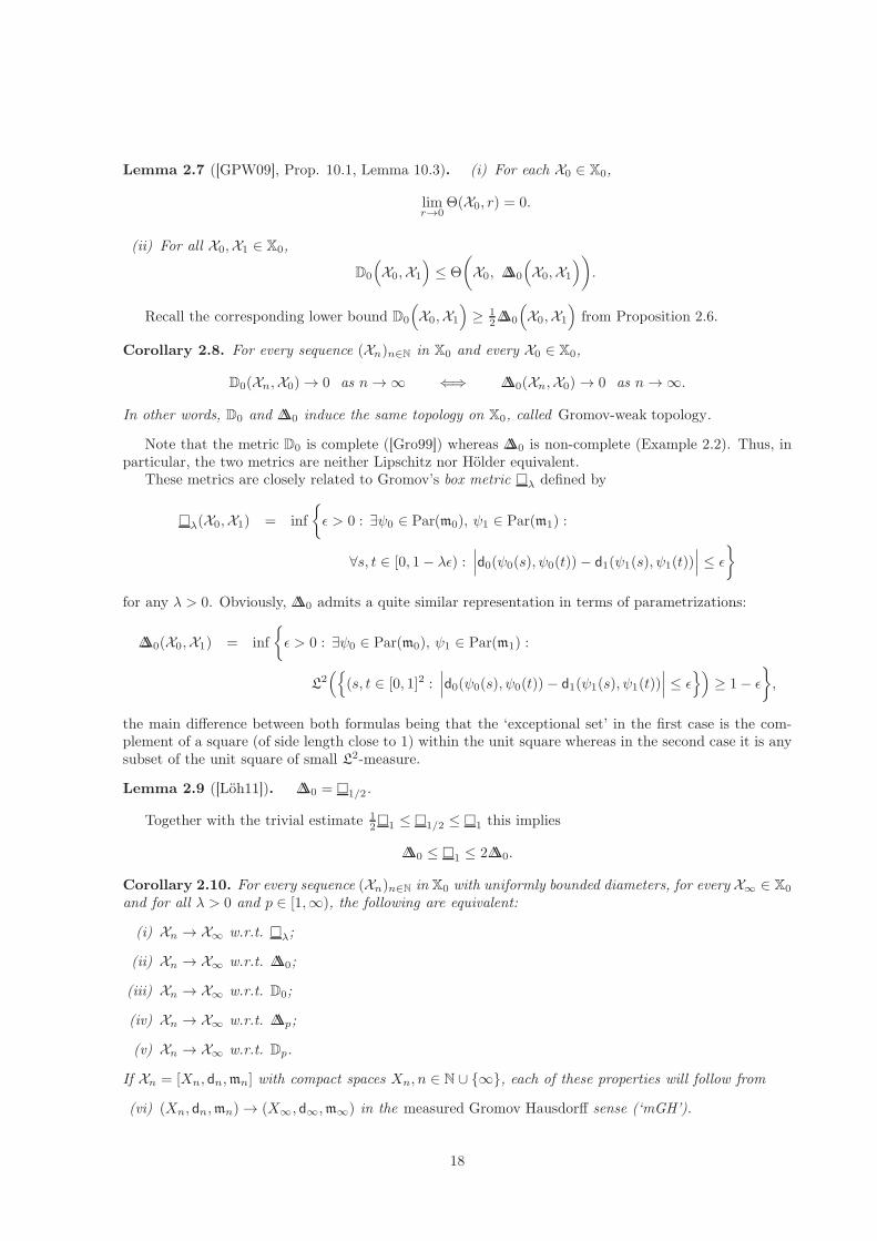
Corollary 2.10. For every sequence (Xn)n∈N in X0 with uniformly bounded diameters, for every X∞ ∈ X0

and for all λ > 0 and p ∈ [1,∞), the following are equivalent:

(i) Xn → X∞ w.r.t. λ;

(ii) Xn → X∞ w.r.t. ∆∆0;

(iii) Xn → X∞ w.r.t. D0;

(iv) Xn → X∞ w.r.t. ∆∆p;

(v) Xn → X∞ w.r.t. Dp.

If Xn = [Xn, dn,mn] with compact spaces Xn, n ∈ N ∪ ∞, each of these properties will follow from

(vi) (Xn, dn,mn) → (X∞, d∞,m∞) in the measured Gromov Hausdorff sense (‘mGH’).

18

Conversely, any of the properties (i)-(v) will imply (vi) provided the spaces (Xn, dn,mn) have full supportand satisfy uniform bounds for doubling constants and diameters.

Proof. For the relation between Dp- and mGH-convergence we refer to [Stu06], Lemma 3.18. The rest isobvious by the previous discussions.

Remarks 2.11. • The history of mm-spaces essentially starts with Gromov’s monograph [Gro99], moreprecisely, the famous Chapter 3 1

2 therein. He promoted very much the idea of focussing on propertieswhich are invariant under isomorphisms. He also introduced several distances on X, among others,the box distance λ. (Even before that, the topology of mGH-convergence on the space of mm-spaces was introduced by Fukaya [Fuk87]. The concept of mGH-convergence, however, is notcompatible with the equivalence relation of isomorphism classes.)

• The Lp-transportation distance Dp was introduced and discussed in detail (mainly restricted to thecase p = 2) by the author in [Stu06].

• Both the L0-transportation distance and the L0-distortion distance ∆∆0 were introduced by Greven,Pfaffelhuber and Winter [GPW09]. They called them Gromov-Prohorov metric and Eurandommetric, resp. Indeed, they derived an equivalent formulation for ∆∆0 in the spirit of the usualdefinition of the Prohorov distance. They also introduced the L1-distortion distance ∆∆1 (at least fortruncated d’s) and gave Example 2.2 (with non-optimal constants). The Gromov-Prohorov metricand its relation to the so-called Gromov-Hausdorff-Prohorov metric were discussed in [Vil09].

• The space X serves as an important model in image analysis and shape matching. In a series ofpapers, Memoli introduced and analyzed various distances (partly for finite, partly for compactmm-spaces) with emphasis on computational aspects and in view of applications to shape matchingand object recognition. In [Mém11], he presented an exhaustive survey on the distances ∆∆p andDp (which he denoted by 2Dp and Sp, resp.), their mutual relations and applications in imageanalysis. Among others, he deduced a slightly restricted version of Proposition 1.12 (i.e. restrictedto compact mm-spaces) as well as several estimates of Proposition 2.6 (partly with non-optimalconstants).

• In recent years, the concept of mm-spaces and related topological/metric issues on the space X foundsurprising new applications in the study of random graphs and their limits, e.g. the continuumrandom tree or the Brownian map, see e.g. [GPW09], [ADH12], [LG10] and [Mie07].

In none of the previous works, any geometric properties of the space X itself have been derived. (Theonly exception might be [Stu06] where geodesics had been characterized.) From our point of view, theemphasis of this paper is not on the ‘metric results’ from the previous chapters but on the ‘geometricresults’ (concerning geodesics, curvature, quasi-Riemannian tangent structure etc.) of the subsequentchapters.

3 Geodesics in (Xp,∆∆p)

Recall that (as usual in metric geometry) a curve (Xt)t∈J – where J denotes some interval in R – is calledgeodesic if ∀S, s, t, T ∈ J with S < s < t < T :

∆∆p(Xs,Xt) =t− s

T − S∆∆p(XS ,XT ).

Thus, by definition, geodesics are always distance minimizing and have constant speed.

Theorem 3.1. For each p ∈ [1,∞],(Xp,∆∆p

)is a geodesic space. More specifically, the following

assertions hold:

(i) For each pair of mm-spaces X0,X1 ∈ Xp and each optimal coupling m of them (cf. Definition 1.8),the family of metric measure spaces

Xt = [X0 ×X1, dt, m], t ∈ (0, 1),

19

withdt ((x0, x1), (y0, y1)) := (1− t)d0(x0, y0) + td1(x1, y1)

defines a geodesic (Xt)0≤t≤1 in Xp connecting X0 and X1.

(ii) If p ∈ (1,∞), then each geodesic (Xt)0≤t≤1 in Xp is of the form as stated in (i). That is, for eachgeodesic (Xt)0≤t≤1 there exists an optimal coupling m of the measures m0,m1, defined on the productspace of (X0, d0,m0) and (X1, d1,m1), representatives of the endpoints, such that for each t ∈ (0, 1)a representative of the isomorphism class Xt is given by (X0 ×X1, dt,m) with dt := (1− t)d0 + td1.

Note that in the case p ∈ (1,∞) a conclusion from (ii) is that geodesics (Xt)0≤t≤1 in Xp do not branchat times t 6= 0, 1. And they do not collapse to atoms at interior points. More precisely,

Corollary 3.2. If (Xt)t∈[0,1] and (X ′t)t∈[0,1] are two non-identical geodesics in Xp (for 1 < p <∞) withidentical initial and terminal points (i.e. X0 = X ′0,X1 = X ′1 and Xt 6= X ′t for some t ∈ (0, 1)) then noneof these geodesics can be extended to a geodesic beyond t = 0 or t = 1.

Corollary 3.3. If the initial point X0 of a geodesic (Xt)t∈[0,1] in Xp (for 1 < p <∞) has no atoms theneach inner point Xt, t ∈ (0, 1), of the geodesic has no atoms.

Proof of the theorem. (i) In order to prove that (Xt)0≤t≤1 is a geodesic in Xp, it suffices to verify that

∆∆p(Xs,Xt) ≤ |s− t|∆∆p(X0,X1)

for all s, t ∈ [0, 1]. We will restrict the discussion to the case p < ∞. For a given pair s, t ∈ (0, 1), notethat the ‘diagonal coupling’

d ¯m(x, y) := dδx(y)dm(x)

is one of the possible couplings of the measures of Xs and Xt (both being m). Thus, with X := X0 ×X1

∆∆p(Xs,Xt)p ≤

∫

X×X

∫

X×X|ds(x, y)− dt(x

′, y′)|p d ¯m(x, x′)d ¯m(y, y′)

=

∫

X

∫

X

|ds(x, y)− dt(x, y)|p dm(x)dm(y)

= |s− t|p∫

X

∫

X

|d0(x0, y0)− d1(x1, y1)|p dm(x0, x1)dm(y0, y1)

= |s− t|p∆∆p(X0,X1)p.

In the case s = 0 and t ∈ (0, 1), a slight modification of the argument is requested. Now we choose

d ¯m(x0, y) := dδy0(x0)dm(y)

(where y = (y0, y1)) as one of the possible couplings of the measures m0 of X0 and m of Xt. Then theargument works as before. Similarly, for the case s ∈ (0, 1) and t = 1.

(ii) Let a geodesic (Xt)0≤t≤1 in Xp be given. Fix a number k ∈ N and let µi (for i = 1, . . . , 2k) beoptimal couplings of the measures m(i−1)2−k and mi2−k . Glue together all these couplings to obtain aprobability measure

µ = µ1 ⊠ µ2 ⊠ . . .⊠ µ2k

on X0 ×X2−k × . . .×Xi2−k × . . .×X1. Put m = (π0, π1)∗µ as well as mt = (π0, πt, π1)∗µ for all t ∈ (0, 1)of the form t = i2−k (for i = 1, . . . , 2k − 1). Thus m is a coupling of m0 and m1 (a priori not optimal).

20

Let us now first restrict to the case p ≥ 2. Then for each t = i2−k (for some i = 1, . . . , 2k − 1),

∆∆p(X0,X1)p

(∗)≤

∫ ∫ ∣∣∣d0(x0, y0)− d1(x1, y1)∣∣∣p

dm(x0, x1)dm(y0, y1)

=

∫ ∫ ∣∣∣[d0(x0, y0)− dt(xt, yt)

]+[dt(xt, yt)− d1(x1, y1)

]∣∣∣p

dmt(x0, xt, x1)dmt(y0, yt, y1)

(∗∗)≤

∫ ∫ [ 1

tp−1∣∣d0(x0, y0)− dt(xt, yt)

∣∣p + 1

(1− t)p−1∣∣dt(xt, yt)− d1(x1, y1)

∣∣p]dmt(x0, xt, x1)dmt(y0, yt, y1)

− 1

C[t(1 − t)]p−1

∫ ∫ ∣∣∣(1 − t)[d0(x0, y0)− dt(xt, yt)

]− t[dt(xt, yt)− d1(x1, y1)

]∣∣∣p

dmt(x0, xt, x1)dmt(y0, yt, y1)

= (I) − (II).

The last inequality (∗∗) is based on the estimate (ii) of Lemma 3.4 below, applied pointwise to theintegrand taking a = d0−dt

t and b = dt−d11−t . In the case p = 2, it is even an equality with C = 1.

Let us have a closer look on the first integral (I). Using estimate (i) of the Lemma below, it can bebounded from above as follows

(I) = 2k(p−1)∫ ∫ [

1

ip−1∣∣d0(x0, y0)− di2−k(xi2−k , yi2−k)

∣∣p + 1

(2k − i)p−1∣∣di2−k(xi2−k , yi2−k)− d1(x1, y1)

∣∣p]

dµ(x0, . . . , xi2−k , . . . , x1)dµ(y0, . . . , yi2−k , . . . , y1)

≤ 2k(p−1)2k∑

j=1

∫ ∫ ∣∣∣d(j−1)2−k(x(j−1)2−k , y(j−1)2−k)− dj2−k(xj2−k , yj2−k)∣∣∣p

dµ(x0, . . . , x(j−1)2−k , xj2−k , . . . , x1)dµ(y0, . . . , y(j−1)2−k , yj2−k , . . . , y1)

= 2k(p−1)2k∑

j=1

∆∆p(X(j−1)2−k ,Xj2−k )p

= ∆∆p(X0,X1)p.

This allows two conclusions: i) The coupling m of m0 and m1 is optimal since the very first inequality (∗)must be an equality. ii) The second integral (II) in the above derivation must vanish. That is,∫

X0×Xt×X1

∫

X0×Xt×X1

∣∣∣(1− t)d0(x0, y0) + td1(x1, y1)− dt(xt, yt)∣∣∣p

dmt(x0, xt, x1)dmt(y0, yt, y1) = 0.

Since mt is a coupling of m and mt, this implies that the mm-spaces (Xt, dt,mt) and (X0×X1, (1− t)d0+td1, m) are isomorphic. This holds true for any t ∈ (0, 1) of the form t = i2−k for some i = 1, . . . , 2k − 1.

Now let us consider the case p ≤ 2 which requires a slightly modified argumentation. Here we considerthe Lp-distortion distance to the power 2. It yields

∆∆p(X0,X1)2

≤(∫ ∫ ∣∣∣

[d0(x0, y0)− dt(xt, yt)

]+[dt(xt, yt)− d1(x1, y1)

]∣∣∣p

dmt(x0, xt, x1)dmt(y0, yt, y1)

)2/p

(∗∗∗)≤ 1

t

(∫ ∫ [∣∣d0(x0, y0)− dt(xt, yt)∣∣p]dmt(x0, xt, x1)dmt(y0, yt, y1)

)2/p

+1

1− t

(∫ ∫ [∣∣dt(xt, yt)− d1(x1, y1)∣∣p]dmt(x0, xt, x1)dmt(y0, yt, y1)

)2/p

− p− 1

t(1− t)

(∫ ∫ ∣∣∣(1− t)[d0(x0, y0)− dt(xt, yt)

]− t[dt(xt, yt)− d1(x1, y1)

]∣∣∣p

dmt(x0, xt, x1)dmt(y0, yt, y1)

)2/p

= (I′) − (II′).

21

Now the last inequality (∗∗∗) is based on the estimate (iii) of Lemma 3.4 below, applied to the Lp-norms(w.r.t. the measure m2

t ) of the involved functions.The quantity (I′) can be estimated similarly as before, using the triangle inequality for the Lp-norm

and estimate (i) of Lemma 3.4 with p = 2:

(I′) =2k

i

(∫ ∫ ∣∣d0(x0, y0)− di2−k(xi2−k , yi2−k)∣∣p

dµ(x0, . . . , xi2−k , . . . , x1)dµ(y0, . . . , yi2−k , . . . , y1)

)2/p

+2k

2k − i

(∫ ∫ ∣∣di2−k(xi2−k , yi2−k)− d1(x1, y1)∣∣p

dµ(x0, . . . , xi2−k , . . . , x1)dµ(y0, . . . , yi2−k , . . . , y1)

)2/p

≤ 2k2k∑

j=1

(∫ ∫ ∣∣∣d(j−1)2−k (x(j−1)2−k , y(j−1)2−k)− dj2−k(xj2−k , yj2−k)∣∣∣p

dµ(x0, . . . , x(j−1)2−k , xj2−k , . . . , x1)dµ(y0, . . . , y(j−1)2−k , yj2−k , . . . , y1)

)2/p

= 2k2k∑

j=1

∆∆p(X(j−1)2−k ,Xj2−k )2

= ∆∆p(X0,X1)2.

This allows the very same conclusions as before: i) the coupling is optimal and ii) the mm-spaces(Xt, dt,mt) and (X0 ×X1, (1− t)d0 + td1, m) are isomorphic.

To indicate the dependence on k, let us now denote the optimal coupling m (obtained via the aboveconstruction) by m(k). According to Lemma 1.2, the family (m(k))k∈N has an accumulation point m(∞)

in Cpl(m0,m1). With this m(∞) in the place of the previous m(k) it follows that for all dyadic numberst ∈ (0, 1), the mm-spaces (Xt, dt,mt) and (X0 ×X1, (1− t)d0 + td1, m

(∞)) are isomorphic. Continuity ofboth as elements in X in t finally allows to conclude this identification for all t ∈ (0, 1).

In the previous proof we used the following basic estimates between real numbers, partly known asClarkson’s inequalities.

Lemma 3.4. (i) ∀p ∈ (1,∞), ∀t0 < t1 . . . < tn, ∀a1, . . . , an ∈ R+

1

(tn − t0)p−1

( n∑

i=1

ai

)p≤

n∑

i=1

1

(ti − ti−1)p−1api .

(ii) ∀p ∈ [2,∞), ∀t ∈ (0, 1) : ∃C = C(p, t) > 0 : ∀a, b ∈ R

|ta+ (1− t)b|p ≤ t|a|p + (1− t)|b|p − t(1 − t)

C|a− b|p.

(iii) For all p ∈ (1, 2], all t ∈ (0, 1), all probability spaces (Ω,A,P) and all f, g ∈ Lp(Ω,P),

‖tf + (1− t)g‖2p ≤ t‖f‖2p + (1− t)‖g‖2p − (p− 1)t(1− t)‖f − g‖2p.

Proof. (i) Consequence of Jensen’s inequality applied to numbers ai

ti−ti−1and weights λi =

ti−ti−1

tn−t0 with∑i λi = 1.For (ii) and (iii), see e.g. Prop. 3 of [BCL94]. (ii) is the quantitative version of the uniform convexity

of r 7→ rp for p ≥ 2. (iii) is the 2-convexity of the Lp-norm for p ≤ 2. Actually, both inequalities arestated only for t = 1

2 . However, a simple iteration argument allows to deduce them for arbitrary dyadict (with the optimal constant in case of (iii) and with some constant C(p, t) > 0 in case of (ii)).

22

Remark 3.5. Given a mm-space X0 we say that another mm-space X1 is a regular target for X0 if thereexists a measurable map φ : X0 → X1 such that

m = (Id, φ)∗m0

is a coupling of m0 and m1 which is optimal for ∆∆p. In other words, X1 is a regular target for X0 if thereexists a measurable map φ with φ∗m0 = m1 such that

∆∆p(X0,X1)p =

∫

X0

∫

X0

|d0(x, y)− d1(φ(x), φ(y))|p dm0(x)dm0(y). (3.1)

A geodesic (Xt)0≤t≤1 emanating from X0 is called regular (for X0) if it connects X0 with some regulartarget X1. Such a geodesic can be represented on the state space of X0 as

Xt =[X0, (1− t)d0 + t φ∗d1,m0

]

where φ∗d1 denotes the pull back of d1 from X1 to X0 through φ, that is, φ∗d1(x0, y0) = d1(φ(x0), φ(y0)).This is in analogy to the ‘classical’ theory of optimal transportation where in ‘nice situations’ the

(unique) solution to the Kantorovich problem coincides with the solution to the Monge problem. Note,however, that there is a significant difference to the ‘classical’ theory of optimal transportation on Eu-clidean or Riemannian spaces.

• ‘Nice’ points µ0 of the Wasserstein space Pp(X) on a Riemannian manifold X have the propertythat each target µ1 ∈ Pp(X) is regular for µ0. For instance, all probability measures µ0 which areabsolutely continuous with respect to the volume measure on X are ‘nice’.

• In contrast to that, even for ‘nice’ points in Xp like smooth compact Riemannian manifolds, e.g.n-dimensional spheres Sn, we expect that there are plenty of non-regular targets, e.g. productsSn × Sk.

Challenge 3.6. (i) Prove the existence (and uniqueness) of such a transport map φ between ‘nice’spaces (e.g. smooth compact Riemannian manifolds of the same dimension) – i.e. Xp-version ofBrenier [Bre91] and McCann [McC01];

(ii) Derive regularity and smoothness results for this map – i.e. Xp-version of Ma, Trudinger, Wang[MTW05].

(iii) Let X0 = (X0, d0,m0) and X1 = (X1, d1,m1) be smooth Riemannian manifolds equipped with theirRiemannian distances and with some weighted volume measures m0 and m1, resp. Assume thatthere exists a diffeomorphism φ : X0 → X1 with m1 = φ∗m0 and satisfying (3.1). Prove or disprove:each of the points

Xt =[X0, (1− t)d0 + t φ∗d1,m0

]

on the geodesic (Xt)0≤t≤1 connecting X0 and X1 is a smooth Riemannian manifold (with Rieman-nian distance and weighted volume measure).

Why should this be true (and why is it not obvious)? Let gi denote the metric tensor on the manifoldXi (i = 0, 1). Then the pull back metric tensor

φ∗g1

defines another metric tensor onX0, compatible with the pull back distance φ∗d1. Unfortunately, however,the convex combination of the metric tensors g0 and φ∗g1 does not lead to a convex combination of theRiemannian distances d0 and φ∗d1. It is unclear whether these latter convex combination is a Riemanniandistance (i.e. whether it is associated with some metric tensor).

Definition 3.7. A metric measure space (X, d,m) is called geodesic mm-space if for all x, y ∈ supp(m)there exists a curve γ : [0, 1] → X with γ0 = x, γ1 = y and length(γ) = d(x, y).

(X, d,m) is called length mm-space if for all x, y ∈ supp(m)

d(x, y) = inflength(γ) : γ0 = x, γ1 = y

.

23

It is easy to see that being a geodesic (or length) mm-space is a property of the isomorphism class[X, d,m]. The space of all isomorphism classes of geodesic mm-spaces will be denoted by Xgeo and thespace of all length mm-spaces by Xlength.

Proposition 3.8. Xgeo and Xlength are convex subsets of X.

Proof. Obviously, a mm-space (X, d,m) is a geodesic (or length) mm-space if and only if the metric space(supp(m), d) is a geodesic (or length, resp.) space in the usual sense of metric geometry, see e.g. [BBI01].To simplify the presentation, let us assume without restriction that m has full support. It is well-knownthat (X, d) is a geodesic (or length, resp.) space if and only if for each pair (x, y) ∈ X2 there exists amidpoint M(x, y) (or a sequence of 1/n-midpoints Mn(x, y), resp.) characterized by

d(x,M(x, y)) = d(y,M(x, y)) =1

2d(x, y)

(or d(x,Mn(x, y)) ≤ (12 + 1n )d(x, y) and d(y,Mn(x, y)) ≤ (12 + 1

n )d(x, y), resp.).Now let two geodesic mm-spaces [X0, d0,m0] and [X1, d1,m1] be given. Assume without restriction

that the chosen representatives have full support. Let

M0 : X20 → X0, M1 : X2

1 → X1

be the midpoint maps and define

M :(X0 ×X1)

2 → X0 ×X1((x0, x1), (y0, y1)

)7→

(M0(x0, y0),M1(x1, y1)

).

Then for each t ∈ (0, 1) and each m ∈ Cpl(m0,m1), M is a midpoint map for (X0 × X1, dt, m) withdt = (1 − t)d0 + td1. Indeed,

dt(x,M(x, y)) = (1 − t)d0(x0,M0(x0, y0)) + td1(x1,M1(x1, y1))

= (1 − t)1

2d0(x0, y0) + t

1

2d1(x1, y1)

=1

2dt(x, y)

and also dt(y,M(x, y)) = 12dt(x, y).

Essentially the same argumentation applies to 1/n-midpoint maps in the case of length spaces.

Remarks 3.9. (i) Since the set of all possible midpoints is closed the measurable selection theoremprovides a Borel measurable map M : X2 → X such that for each x, y ∈ X2 the point M(x, y) is amidpoint of x and y, provided of course X is a geodesic space. Similarly, for each n ∈ N it providesa Borel measurable 1/n-midpoint map on a given length space.

(ii) Neither Xgeo nor Xlength is closed. An easy counterexample is provided by the sequence of geodesicmm-spaces [[

I, |.|, 1nL1 +

1

2(1− 1

n)δ0 +

1

2(1− 1

n)δ1

]]

which ∆∆p-converges to [[I, |.|, 1

2δ0 +

1

2δ1

]].

4 Cone Structure and Curvature Bounds for (X,∆∆)

4.1 Cone Structure

From now on, for the rest of the paper we will restrict ourselves to the case p = 2. We simply write X

instead of X2, ∆∆ instead of ∆∆2, and size(.) instead of size2(.).We begin with a reformulation of the L2-distortion distance which is analogous to the reformulations

of the classical transport problem for the cost functions |x − y|2 in terms of the transport problem forthe cost function −2xy. Indeed, such a result only holds for p = 2.

24

Proposition 4.1. ∀X0,X1 ∈ X:

∆∆(X0,X1)2 =size(X0)

2 + size(X1)2

− 2 sup

∫

X0×X1

∫

X0×X1

d0(x0, y0)d1(x1, y1)dm(x0, x1)dm(y0, y1) : m ∈ Cpl(m0,m1)

.

Proof. Decompose the integrand |d0(x0, y0) − d1(x1, y1)|2 in the integrals used in the definition of ∆∆2

into two squares of distances and a midterm. Then observe that each of the integrals of a distance squareonly depends on one of the marginals of m, e.g.

∫

X0×X1

∫

X0×X1

d0(x0, y0)2dm(x0, x1)dm(y0, y1) =

∫

X0

∫

X0

d0(x0, y0)2dm(x0)dm(y0) = size(X0)

2.

The space X0 has a distinguished element: the isomorphism class of metric measure spaces (X, d,m)whose support consist of one point, say x ∈ X (and thus m = δx). This isomorphism class will be called1-point space and denoted by δ. Note that for each X ∈ X0,

size(X ) = ∆∆(δ,X )

and thusX

1 := X ∈ X : size(X ) = 1is the unit sphere in (X,∆∆) around δ. Given any X1 = [X1, d1,m1] ∈ X, the unique unit speed geodesicthrough X1 and emanating from δ is given by

Xt = [X1, td1,m1].

It is called ray through X1. Each element X 6= δ in X can uniquely be characterized as a pair (r,X1) ∈(0,∞)×X1. The number r is the size of X , the element X1 ∈ X1 is the ‘standardization’ of X = [X, d,m]:

X1 := [X,d

size(X ),m].

A remarkable, quite surprising fact is that the L2-distortion distance between two spaces X = (r,X1)and X ′ = (r′,X ′1) is completely determined by the sizes r = size(X ), r′ = size(X ′) and the distance∆∆(X1,X ′1) of the standardized spaces.

Lemma 4.2. Let X1,X ′1 ∈ X1 and let (Xs)s≥0, (X ′t )t≥0 be the corresponding rays. Then the quantity

1

2st

[∆∆2(Xs,X ′t )− s2 − t2

]

is independent of s, t ∈ (0,∞).

Proof. Let the rays be given as Xs = (X, sd,m) and X ′t = (X ′, td′,m′). Then for each m ∈ Cpl(m,m′)and all s, t ∈ (0,∞):

1

2st

[∫

X×X′

∫

X×X′

|sd(x, y)− td′(x′, y′)|2 dm(x, x′)dm(y, y′)− s2 − t2]

=1

2st

[s2∫

X

∫

X

d(x, y)2dm(x)dm(y)− s2

+ t2∫

X′

∫

X′

d′(x′, y′)2dm′(x′)dm′(y′)− t2

−2st

∫

X×X′

∫

X×X′

d(x, y)d′(x′, y′)dm(x, x′)dm(y, y′)

]

=−∫

X×X′

∫

X×X′

d(x, y)d′(x′, y′)dm(x, x′)dm(y, y′),

which obviously is independent of s and t. The last equality is due to the fact that size(X ) = 1 as wellas size(X ′) = 1.

25

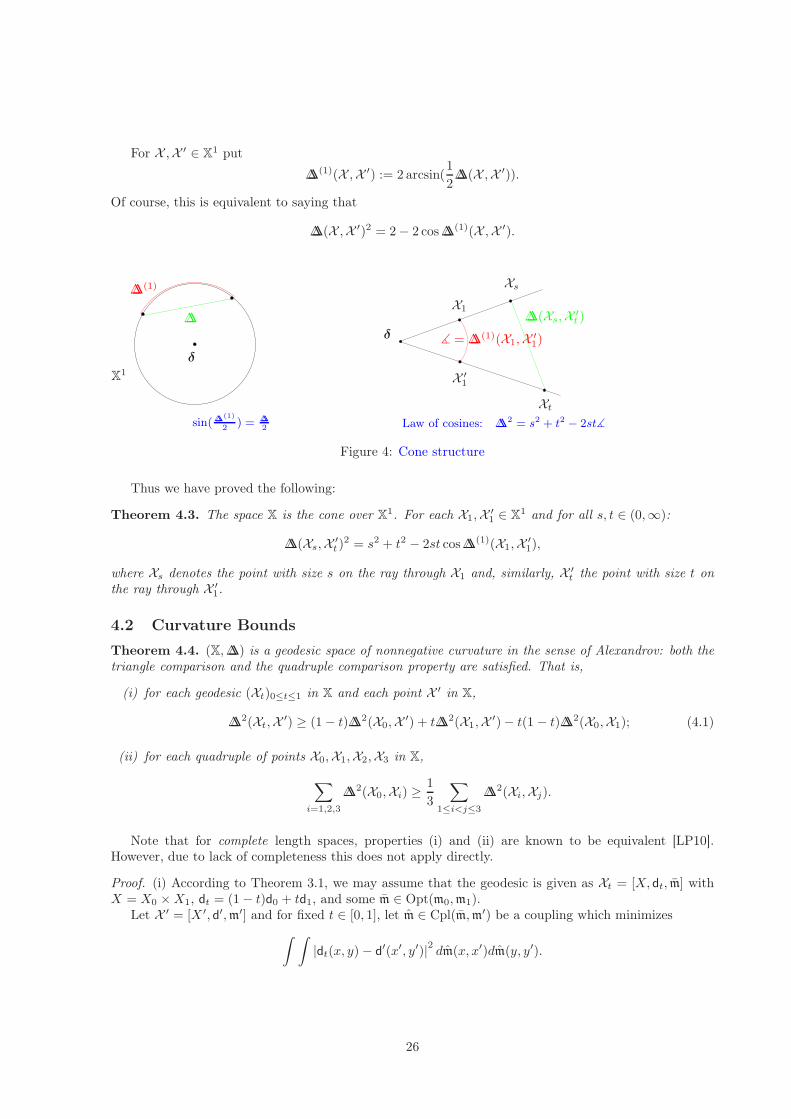
For X ,X ′ ∈ X1 put

∆∆(1)(X ,X ′) := 2 arcsin(1

2∆∆(X ,X ′)).

Of course, this is equivalent to saying that

∆∆(X ,X ′)2 = 2− 2 cos∆∆(1)(X ,X ′).

δ

X1

∆∆

∆∆(1)

sin(∆∆(1)

2) = ∆∆

2

X1

Xs

Xt

X ′1

δ ∡ = ∆∆(1)(X1,X ′1)∆∆(Xs,X ′t )

Law of cosines: ∆∆2 = s2 + t2 − 2st∡

Figure 4: Cone structure

Thus we have proved the following:

Theorem 4.3. The space X is the cone over X1. For each X1,X ′1 ∈ X

1 and for all s, t ∈ (0,∞):

∆∆(Xs,X ′t )2 = s2 + t2 − 2st cos∆∆(1)(X1,X ′1),

where Xs denotes the point with size s on the ray through X1 and, similarly, X ′t the point with size t onthe ray through X ′1.

4.2 Curvature Bounds

Theorem 4.4. (X,∆∆) is a geodesic space of nonnegative curvature in the sense of Alexandrov: both thetriangle comparison and the quadruple comparison property are satisfied. That is,

(i) for each geodesic (Xt)0≤t≤1 in X and each point X ′ in X,

∆∆2(Xt,X ′) ≥ (1− t)∆∆2(X0,X ′) + t∆∆2(X1,X ′)− t(1 − t)∆∆2(X0,X1); (4.1)

(ii) for each quadruple of points X0,X1,X2,X3 in X,

∑

i=1,2,3

∆∆2(X0,Xi) ≥1

3

∑

1≤i<j≤3∆∆2(Xi,Xj).

Note that for complete length spaces, properties (i) and (ii) are known to be equivalent [LP10].However, due to lack of completeness this does not apply directly.

Proof. (i) According to Theorem 3.1, we may assume that the geodesic is given as Xt = [X, dt, m] withX = X0 ×X1, dt = (1− t)d0 + td1, and some m ∈ Opt(m0,m1).

Let X ′ = [X ′, d′,m′] and for fixed t ∈ [0, 1], let m ∈ Cpl(m,m′) be a coupling which minimizes

∫ ∫|dt(x, y)− d′(x′, y′)|2 dm(x, x′)dm(y, y′).

26

X0

X1Xt

X ′

Triangle comparison

a1a2

a3

b1

b2

b3

Quadruple comparison:∑

a2i ≥

13

∑b2i

Figure 5: Nonnegative curvature

In other words, m is a probability measure on X = X ×X ′ which couples m and m′ in an optimal wayw.r.t. ∆∆. Then

∆∆2(Xt,X ′) + t(1− t)∆∆2(X0,X1)

=

∫

X

∫

X

|dt(x, y)− d′(x′, y′)|2 dm(x, x′)dm(y, y′) + t(1 − t)

∫

X

|d0(x, y)− d1(x, y)|2 dm(x)dm(y)

=

∫

X

∫

X

[|(1− t)d0(x, y) + td1(x, y)− d′(x′, y′)|2 + t(1− t) |d0(x, y)− d1(x, y)|2

]dm(x, x′)dm(y, y′)

=

∫

X

∫

X

[(1 − t) |d0(x0, y0)− d′(x′, y′)|2 + t |d1(x1, y1)− d′(x′, y′)|2

]dm(x0, x1, x

′)dm(y0, y1, y′)

≥ (1 − t)∆∆2(X0,X ′) + t∆∆2(X1,X ′),

where the last inequality follows from the fact that (π0, π2)∗m is a coupling of m0 and m′ - but notnecessarily an optimal one for ∆∆. Similarly, for (π1, π2)∗m and m1, m

′.

(ii) Given points X0, . . . ,X3 ∈ X, choose mi ∈ Opt(m0,mi) and define (according to Lemma 1.5) ameasure µ on X = X0 ×X1 ×X2 ×X3 by

dµ(x0, x1, x2, x3) = dm1,x0(x1) dm2,x0(x2) dm3,x0(x3) dm0(x0)

where dmi,x0(xi) denotes the disintegration of dmi(x0, xi) w.r.t. dm0(x0). Then

3∑

i=1

∆∆2(X0,Xi) =

∫

X

∫

X

3∑

i=1

∣∣d0(x0, y0)− di(xi, yi)∣∣2dµ(x) dµ(y)

≥∫

X

∫

X

1

3

∑

1≤i<j≤3

∣∣di(xi, yi)− dj(xj , yj)∣∣2dµ(x) dµ(y)

≥ 1

3

∑

1≤i<j≤3∆∆2(Xi,Xj).

The last inequality here comes from the fact that for all i, j ∈ 1, 2, 3

(πi, πj)∗µ ∈ Cpl(mi,mj)

but is not necessarily optimal. The first inequality follows from the quadruple inequality in the metricspace (R1, |.|) applied to the 4 points ξi = di(xi, yi), i = 0, 1, 2, 3, for each fixed pair (x, y) ∈ X2.

Corollary 4.5. The metric completion (X,∆∆) of (X,∆∆) is a complete length space of nonnegative cur-vature in the sense of Alexandrov.

Obviously, also X is a cone over its unit sphere X1 (which is the completion of X1).

Proof. The quadruple inequality immediately carries over to the completion. According to [LP10], forcomplete length spaces this characterizes nonnegative curvature in the sense of Alexandrov.

Corollary 4.6. (i) (X1,∆∆(1)) is a complete length space with curvature ≥ 1 in the sense of Alexandrov.

27

(ii) (X1,∆∆(1)) is a geodesic space with curvature ≥ 1: both the triangle and the quadruple comparisonproperty are satisfied.

Proof. (i) It is a well-known fact from geometry of Alexandrov spaces, see e.g. [BBI01], Thm. 10.2.3.,that cone structure together with nonnegative curvature implies that the unit sphere has curvature ≥ 1.This result immediately applies to the completion X and its unit sphere X1.

(ii) The fact that (X1,∆∆(1)) is a geodesic space follows from Theorem 4.3 (‘cone structure’) togetherwith the fact that (X,∆∆) itself is a geodesic space. The triangle and the quadruple inequality now bothfollow from (i) by applying it to points in X1.

4.3 Space of Directions, Tangent Cone, and Gradients on X

According to the previous Corollary 4.6, (X,∆∆) is a complete length space of nonnegative curvature.Indeed, we will see in Theorem 5.21 that (X,∆∆) is even a geodesic space (not just a length space). Asconsequences of general results on Alexandrov spaces this implies a variety of existence and structuralresults on tangent cones, exponential maps and gradients. We present some of the basic concepts andresults, following mainly [Pla02]. We formulate these definitions and assertions for the particular space(X,∆∆). Actually, however, they will be true for arbitrary complete geodesic spaces of lower boundedcurvature. The crucial point is that no (local) compactness is required.

The space of geodesic directions at X0 – denoted by T 1X0X – consists of equivalence classes of unit

speed geodesics emanating from X0 where two such geodesics (Xt)0≤t≤τ and (X ′t )0≤t≤τ ′ are regarded asequivalent if one of them is an extension of the other one, say e.g. τ ′ ≥ τ and

Xt = X ′t for t ≤ τ.

The space of geodesic directions is a metric space with a metric ∡ given by

∡(X•,X ′•) = lims,tց0

arccos

[1

2st

(s2 + t2 −∆∆2(Xs,X ′t )

)].

The limit always exists. Indeed, as a consequence of the curvature bound, the quantity arccos[.] in theabove formula is non-increasing in s and in t. The space of directions at X0 – denoted by T 1

X0X – is the

completion of the space of geodesic directions at X0 w.r.t. the metric ∡. The tangent cone TX0X at X0 isthe cone over the space of directions at X0.

Definition 4.7. (i) Given a number λ ∈ R, a function U : X → R will be called λ-Lipschitz continuousif

|U(X0)− U(X1)| ≤ λ ·∆∆(X0,X1)

for all X0,X1 ∈ X. In this case, we briefly write Lip(U) ≤ λ. The function U is called Lipschitzcontinuous if it is λ′-Lipschitz continuous for some λ′.

(ii) Given a number κ ∈ R, the function U : X → R is called κ-convex if for all geodesics (Xt)0≤t≤1 inX and for all t ∈ [0, 1],

U(Xt) ≤ (1− t)U(X0) + tU(X1)−κ

2t(1− t)∆∆2(X0,X1).

(Note that if U is continuous, then the latter is equivalent to d2

dt2U(Xt) ≥ κ ·∆∆2(X0,X1) in distri-butional sense on the interval (0, 1) for each given geodesic.) The function U is called semiconvexif it is κ′-convex for some κ′.

(iii) The function U is called κ-concave (or semiconcave) if −U is (−κ)-convex (or semiconvex, resp.),that is, if U(Xt) ≥ (1 − t)U(X0) + tU(X1) − κ

2 t(1 − t)∆∆2(X0,X1) for all geodesics (Xt)0≤t≤1 in X

and all t ∈ [0, 1].Note that functions which we call κ-concave are called by some other authors (−κ)-concave. The sign

convention is not consistent in the literature.

28

Example 4.8. The function X 7→ −∆∆2(X ,X0) is −2-convex for each X0. The same is true for the function

X 7→ max−∆∆2(X ,Xi) : i = 1, . . . , k

for any given set of points X1, . . . ,Xk ∈ X.

For every Lipschitz continuous, semiconcave function U : X → R the ‘ascending slope’ of U at X ∈ X

is∣∣D+U(X )

∣∣ := lim supX ′→X

[U(X ′)− U(X )]+

∆∆(X ′,X ).

A point X ∈ X is called critical for U if |D+U(X )| = 0. The set XU of critical points for U is a closedsubset of X. Each local maximizer (as well as each local minimizer) is critical for U .

For each geodesic direction Φ ∈ TX0X, say Φ = (Xt)0≤t≤τ , the directional derivative of U in directionΦ

DΦU = limtց0

1

t[U(Xt)− U(X0)]

exists and depends continuously on Φ ∈ TX0X (and thus extends to all of TX0X).

Lemma 4.9. For every Lipschitz continuous, semiconcave function U on X and each point X ∈ X:

(i) |D+U(X )| = supDΦU : Φ ∈ TX X, ‖Φ‖TX X = 1

(ii) If |D+U(X )| 6= 0 then there exists a unique unit vector Φ ∈ TX X such that

∣∣D+U(X )∣∣ = DΦU . (4.2)

The gradient of U at X ∈ X, denoted by ∇U(X ) or more precisely by ∇XU(X ), is now defined as anelement in TX X as follows:

• if X is critical for U , put ∇U(X ) = 0,

• otherwise, put ∇U(X ) := tΦ where Φ ∈ TX X is the unique unit tangent vector satisfying (4.2) andt := |D+U(X )|.

Note that by construction,‖∇U(X )‖TX X

=∣∣D+U(X )

∣∣ .

4.4 Gradient Flows on X

Definition 4.10. A curve X• : [0, L) → X (with L ∈ (0,∞]) is called ascending gradient curve of U orsolution of the (‘upward gradient flow’) differential equation

Xt = ∇U(Xt)

if for all t ∈ [0, L):

limsց0

1

s∆∆(Xt+s,Xt) =

∣∣D+U(Xt)∣∣ (4.3)

and

limsց0

1

s[U(Xt+s)− U(Xt)] =

∣∣D+U(Xt)∣∣2 . (4.4)

Theorem 4.11. Let U : X → R be Lipschitz continuous and κ-concave.

(i) Then for each X0 ∈ X there exists a unique ascending gradient curve (Xt)0≤t<∞ of U .

29

(ii) For all X0,X ′0 ∈ X and every t > 0

∆∆(Xt,X ′t

)≤ eκ t ·∆∆

(X0,X ′0

).

The uniqueness in particular implies that Xt = Xτ for all t ≥ τ where τ = infs ≥ 0 : Xs ∈ XU.

Proof. If X0 ∈ XU , then one possible solution to the gradient flow equation (as defined above) is alwaysgiven by

Xt = X0 (∀t ≥ 0).

For X0 6∈ XU , Plaut [Pla02] as well as Lytchak [Lyt05], based on (unpublished) previous work of Perelmanand Petrunin [PP], proved the existence of gradient flow curves. (The concept of gradient-like curvesused in [Pla02] leads to re-parametrizations of gradient flow curves – at least as long as they do not hitthe closed set XU .) The crucial point is that this existence result does not require any compactness of theunderlying space X. The uniqueness result and exponential Lipschitz bound is taken from [Lyt05].

Remark 4.12. In analysis (PDEs, mathematical physics), instead of the upward gradient flow mostly thedownward gradient flow for a given function U on X is considered.

Xt = ∇(−U)(Xt).

It is just the upward gradient flow for −U . (Note that in metric geometry we have to distinguish between∇(−U) and −∇U .)

This requires the function U now to be semiconvex. The relevant quantity then is the descendingslope

|D−U(X )| = |D+(−U)(X )| = lim supX ′→X

[U(X ) − U(X ′)]+∆∆(X ′,X ).

5 The Space Y of Gauged Measure Spaces

5.1 Gauged Measure Spaces

In order to analyze and characterize elements X in the completion X of the space of mm-spaces, and toobtain a more explicit representation of tangent spaces TX and exponential maps ExpX , we embed thespace of mm-spaces into a bigger space Y which in the sense of Alexandrov geometry is more regular. (Inparticular, it has less boundary.)

Definition 5.1. A gauged measure space is a triple (X, f,m) consisting of a Polish space X , a Borelprobability measure m on X , and a function f ∈ L2

s(X2,m2). The latter denotes the space of symmetric

functions f on X ×X which are square integrable w.r.t. the product measure m⊗m. Any such functionf is called gauge.

This extends the concept of metric measure spaces in two respects: i) the function f replacing thedistance d is no longer requested to satisfy the triangle inequality; ii) even if it did so, it is no longerrequested to induce the (Polish) topology on X . Metric (or gauge) and topology are decoupled to thegreatest possible extent. The only remaining constraint is that f should be measurable w.r.t. the σ-fieldinduced by the topology. To abandon the triangle inequality will make the space of all gauged measurespaces ‘more linear’.

The size of a gauged measure is simply defined as the L2-norm of its gauge function, i.e.

size(X, f,m

)=( ∫

X

∫

X

f2(x, y)dm(x) dm(y))1/2

.

30

Definition 5.2. (i) The L2-distortion distance between two gauged measure spaces (X0, f0,m0) and(X1, f1,m1) is defined by

∆∆((X0, f0,m0), (X1, f1,m1)

)

= inf

(∫

X0×X1

∫

X0×X1

|f0(x0, y0)− f1(x1, y1)|2 dm(x0, x1)dm(y0, y1)

)1/2

: m ∈ Cpl(m0,m1)

.

(ii) Every minimizer m of the above RHS will be called optimal coupling of the given gauged measurespaces. In other words, a coupling m ∈ Cpl(m0,m1) is optimal if

∆∆((X0, f0,m0), (X1, f1,m1)

)=

(∫ ∫|f0 − f1|2 dm dm

)1/2

.

(iii) Two gauged measure spaces (X0, f0,m0) and (X1, f1,m1) are called homomorphic if

∆∆((X0, f0,m0), (X1, f1,m1)

)= 0.

Obviously, this defines an equivalence relation.

Lemma 5.3. (i) Every gauged measure space (X, f,m) is homomorphic to the space (I, f′,L1) for asuitable f′ ∈ L2

s(I2,L2). Indeed, one may choose f′ = ψ∗f for any ψ ∈ Par(m).

(ii) An optimal coupling of (X, f,m) and (I, ψ∗f,L1) is given by (ψ, Id)∗L1.

Proof. Define m = (ψ, Id)∗L1 for ψ ∈ Par(m). Then obviously m is a coupling of m = ψ∗L1 and L1.

Moreover,∫

X×I

∫

X×I|f − f′|2 dm dm =

∫

I

∫

I

|ψ∗f − f′|2 dL1 dL1 = 0

according to our choice f′ = ψ∗f.

Proposition 5.4. For every pair of gauged measure spaces (X0, f0,m0) and (X1, f1,m1) there exists anoptimal coupling, i.e. a measure m ∈ Cpl(m0,m1) which realizes the L2-distortion distance.

Proof. (i) Let us first prove the claim in the particular case X0 = X1 = I and m0 = m1 = L1. Asbefore in the proof of Lemma 1.7 the claim will follow from compactness of the set Cpl(m0,m1) and lower

semicontinuity of the functional m 7→( ∫ ∫ ∣∣f0 − f1

∣∣2dm dm)1/2

on Cpl(m0,m1). The former remains truein this more degenerate setting, i.e. Lemma 1.2 applies without any change. The latter requires morecare and will be the content of the next lemma.

(ii) The case of general X0, X1 and m0,m1 can be reduced to the previous case as follows. Chooseψi ∈ Par(mi) for i = 0, 1 and put f′i = ψi

∗fi. Apply the previous part (i) to deduce the existence of acoupling m ∈ Cpl(L1,L1) which minimizes

(∫

I2

∫

I2

∣∣f′0(x0, y0)− f′1(x1, y1)∣∣2dm(x0, x1) dm(y0, y1)

)1/2

.

Put m = (ψ0, ψ1)∗m. This defines a coupling of m0 and m1 and satisfies(∫

X0×X1

∫

X0×X1

∣∣f0 − f1∣∣2dm dm

)1/2

=

(∫

I2

∫

I2

∣∣ψ∗0 f0 − ψ∗1 f1∣∣2dm dm

)1/2

= ∆∆((I, f′0,L

1), (I, f′1,L1))

≤ ∆∆((I, f′0,L

1), (X0, f0,m0))+∆∆

((X0, f0,m0), (X1, f1,m1)

)+∆∆

((X1, f1,m1), (I, f

′1,L

1))

= ∆∆((X0, f0,m0), (X1, f1,m1)

)

according to the previous lemma. This proves the optimality of m.

31

Lemma 5.5. Given two functions f0, f1 ∈ L2s(I

2,L2), the functional

m 7→ Ξ(m) :=

(∫

I2

∫

I2

∣∣f0(x0, y0)− f1(x1, y1)∣∣2dm(x0, x1) dm(y0, y1)

)1/2

is continuous on Cpl(L1,L1), the latter being regarded as a subset of P(I2) equipped with the topology ofweak convergence.

Proof. Every f ∈ L2s(I

2,L2) can be approximated in L2-norm by continuous symmetric functions on I2.(Just apply the heat kernel or any mollifier to f, see e.g. the construction in the proof of Theorem 5.19.)Thus there exist fi,n ∈ L2

s(I2,L2) ∩ C(I2) for i = 0, 1 and n ∈ N such that

(∫

I

∫

I

∣∣fi(s, t)− fi,n(s, t)∣∣2ds dt

)1/2

≤ 1

n.

For each n ∈ N the functional

m 7→ Ξn(m) :=

(∫

I2

∫

I2

∣∣f0,n(x0, y0)− f1,n(x1, y1)∣∣2dm(x0, x1) dm(y0, y1)

)1/2

is continuous on Cpl(m0,m1) due to the fact that the integrand |f0,n − f1,n|2 is continuous and boundedon I2 × I2. Moreover, by a simple application of the triangle inequality in L2(I2 × I2),

∣∣∣Ξ(m)− Ξn(m)∣∣∣ ≤

(∫

I2

∫

I2

∣∣f0(x0, y0)− f0,n(x0, y0)∣∣2dm(x0, x1) dm(y0, y1)

)1/2

+

(∫

I2

∫

I2

∣∣f1,n(x1, y1)− f1(x1, y1)∣∣2dm(x0, x1) dm(y0, y1)

)1/2

=

(∫

I

∫

I

∣∣f0(s, t)− f0,n(s, t)∣∣2ds dt

)1/2

+

(∫

I

∫

I

∣∣f1,n(s, t)− f1(s, t)∣∣2ds dt

)1/2

≤ 2

n

for each n ∈ N. This proves the continuity of m 7→ Ξ(m) on Cpl(m0,m1).

Proposition 5.6. For any pair of gauged measure spaces (X0, f0,m0) and (X1, f1,m1),

∆∆((X0, f0,m0), (X1, f1,m1)

)= 0 ⇐⇒ ∃(X, f,m), ∃ψi : X → Xi measurable s.t.

(ψi)∗m = mi, (ψi)∗fi = f (∀i = 0, 1).

In particular,

∆∆((X0, f0,m0), (X1, f1,m1)

)= 0 ⇐= ∃ψ : X0 → X1 measurable s.t. ψ∗m0 = m1, ψ

∗f1 = f0.

Here and in the sequel, identities like (ψi)∗fi = f or ψ∗f1 = f0 have to be understood as equalities

m2-a.e. on X2 or m20-a.e. on X2

0 , resp.

Proof. Assume the existence of the space (X, f,m) and the maps ψ0, ψ1 with given properties. Putm = (ψ0, ψ1)∗m. Obviously, this is an element of Cpl(m0,m1) satisfying

∫

X0×X1

∫

X0×X1

∣∣∣f0 − f1

∣∣∣2

dm dm =

∫

X

∫

X

∣∣∣ψ∗0 f0 − ψ∗1 f1∣∣∣2

dm dm = 0.

Now, conversely, assume that ∆∆(., .) = 0. Then according to Proposition 5.4 there exist m ∈ Cpl(m0,m1)with

∫ ∫|f0 − f1|2dm dm = 0. Then

f0(x0, y0) = f1(x1, y1) for m2-a.e.

((x0, x1), (y0, y1)

)∈ X2

for X := X0 ×X1. Thus (X, f, m) with f := 12 f0 +

12 f1 will do the job together with ψi = πi : X → Xi

being the projections (i = 0, 1).

32

Remarks 5.7. (i) If m0 has atoms and m1 has no atoms then there exists no map ψ : X0 → X1 withψ∗m0 = m1.

(ii) For each gauged measure space (X0, f0,m0) there exist gauged measure spaces (X1, f1,m1) without

atoms and with ∆∆((X0, f0,m0), (X1, f1,m1)

)= 0. This follows from Lemma 5.3.

Equivalence classes of homomorphic gauged measure spaces will be denoted by

X0 = [[X0, f0,m0]], X1 = [[X1, f1,m1]], X ′ = [[X ′, f′,m′]] etc.

and their respective representatives as before by (X0, f0,m0), (X1, f1,m1), (X′, f′,m′) etc. The space of

equivalence classes of homomorphic gauged measure spaces will be denoted by Y.

Theorem 5.8. (Y,∆∆) is a complete geodesic space of nonnegative curvature in the sense of Alexandrov.More specifically, the following assertions hold:

(i) For each pair of gauged measure spaces (X0, f0,m0) and (X1, f1,m1), there exists an optimal couplingm ∈ Cpl(m0,m1).

(ii) For each choice of optimal coupling m ∈ Cpl(m0,m1), a geodesic in Y connecting [[X0, f0,m0]] and[[X1, f1,m1]] is given by

Xt = [[X0 ×X1, (1− t)f0 + tf1, m]], t ∈ (0, 1). (5.1)

(iii) Every geodesic (Xt)t∈[0,1] in Y is of this form. That is, given representatives (X0, f0,m0) and(X1, f1,m1) of the endpoints of the geodesic, there exists an optimal coupling m ∈ Cpl(m0,m1)defined on X0 ×X1 such that (5.1) holds.

(iv) (Y,∆∆) satisfies the triangle comparison and the quadruple comparison properties.

(v) (Y,∆∆) is a cone over its unit sphere

Y1 = X ∈ Y : size(X ) = 1.

(vi) Y1 with the induced distance ∆∆(1) is a complete geodesic space with curvature ≥ 1 in the sense ofAlexandrov.

Proof. • Obviously, (Y,∆∆) is a metric space. (Same proof as for Lemma 1.9.)

• The existence of optimal couplings was already stated as Proposition 5.4. The assertions on exis-tence and uniqueness of geodesics thus follow exactly as in Theorem 3.1. None of the argumentsused in the proof required that d is continuous or satisfies the triangle inequality.

• The proof of the cone property from Theorem 4.3 applies without any change.

• All assertions on curvature bounds for Y and Y1 follow with exactly the same arguments as for X

and X1, see Theorem 4.4 and Corollary 4.6.

• It remains to prove the completeness of (Y,∆∆):

Let a sequence of gauged measure spaces (Xn, fn,mn), n ∈ N, be given with

∆∆((Xn, fn,mn), (Xk, fk,mk)

)→ 0 as k, n→ ∞.

Passing to a subsequence if necessary, we may assume that

∆∆((Xn, fn,mn), (Xn+1, fn+1,mn+1)

)≤ 2−n

33

for all n ∈ N which (according to Proposition 5.4) implies the existence of a coupling µn ∈Cpl(mn,mn+1) satisfying

(∫

Xn×Xn+1

∫

Xn×Xn+1

∣∣∣fn − fn+1

∣∣∣2

dµn dµn

)1/2

≤ 2−n. (5.2)

Gluing together all these measures for n = 1, . . . , N − 1 yields a measure

µN = µ1 ⊠ . . .⊠ µN−1 on XN =

N∏

n=1

Xn.

For N → ∞, the projective limitµ = lim

←−µN

of these measures is a probability measure on X =∏∞

n=1Xn with the property

(πn, πn+1)∗µ = µn

for each n ∈ N. Define functions fn ∈ L2s(X

2, µ2) by

fn(x, y) = fn(xn, yn)

for x = (xi)i∈N, y = (yi)i∈N ∈ X . Then

‖fn − fn+1‖L2s(X

2,µ2) = ∆∆((Xn, fn,mn), (Xn+1, fn+1,mn+1)

)≤ 2−n

for all n ∈ N. Therefore, (fn)n is a Cauchy sequence in the Hilbert space L2s(X

2, µ2) and thus there

exists f ∈ L2s(X

2, µ2) with

‖fn − f‖L2s(X

2,µ2) → 0.

The triple (X, f, µ) is the gauged measure space we are looking for. Indeed,

∆∆((Xn, fn,mn), (X, f, µ)

)≤ ‖fn − f‖L2

s(X2,µ2) → 0.

This proves the claim.

5.2 Equivalence Classes in L2

s(I2,L2)

The space Y admits a remarkable and very instructive representation in terms of parametrizations. Forthis purpose, let us consider the semigroup Inv(I,L1) of all Borel measurable maps φ : I → I which leaveL1 invariant, i.e. which satisfy φ∗L1 = L1. This semigroup, call it G for the moment, acts on the linearspace H = L2

s(I2,L2) via pull back

G×H → H

(φ, f) 7→ φ∗f

with(φ∗f

)(s, t) = f

(φ(s), φ(t)

).

Lemma 5.9. G acts isometrically on H.

Proof.

‖φ∗f‖2H =

∫ 1

0

∫ 1

0

∣∣∣f(φ(s), φ(t)

)∣∣∣2

ds dt(∗)=

∫ 1

0

∫ 1

0

∣∣∣f(s, t)∣∣∣

2

ds dt = ‖f‖2H

where (∗) holds due to the L1-invariance of φ.

34

The semigroup G induces an equivalence relation ≃ in H :

f ≃ g ⇐⇒ ∃φ, ψ ∈ G : φ∗f = ψ∗g.

The set of equivalence classes for this relation ≃ will be called quotient space and denoted by

L = H/G = L2s(I

2,L2)/ Inv .

It is a pseudo metric space with pseudo metric dL = dH/G = dL2/ Inv given by

dH/G([[f ]], [[g]]) = inf‖f ′ − g′‖H : f ′ ∈ [[f ]], g′ ∈ [[g]]

= inf‖φ∗f − ψ∗g‖H : φ, ψ ∈ G

.

Here [[f ]] and [[g]] denote the equivalence classes of f, g ∈ H .

Theorem 5.10. (i) (L, dL) is a metric space.

(ii) The metric spaces(L, dL) and (Y,∆∆)

are isometric. An isometry is given by

Θ :L2s(I

2,L2)/ Inv → Y

[[f ]] 7→ [[I, f,L1]].

The inverse map Θ−1 assigns to each representative (X, f,m) of a gauged measure space [[X, f,m]] ∈Y the function f′ = ψ∗f ∈ L2

s(I2,m2) where ψ is any element in Par(m).

(iii) L2s(I

2,L2)/ Inv is a complete geodesic space of nonnegative curvature in the sense of Alexandrov.

Proof. (i), (ii) Let [[f ]], [[g]] ∈ L2s(I

2,L2)/ Inv with representatives f, g in L2s(I

2,L2). Then

dL2/ Inv([[f ]], [[g]]) = inf‖φ∗f − ψ∗g‖L2 : φ, ψ ∈ Inv

≥ ∆∆

((I, f,L1), (I, g,L1)

)= ∆∆

([[I, f,L1]], [[I, g,L1]]

)

since each pair (φ, ψ) ∈ Inv× Inv defines a coupling of L1 with itself via (φ, ψ)∗L1.Conversely, given any coupling m of L1 with itself, there exists φ ∈ Par(m), i.e. φ = (φ0, φ1) : I → I2

such that φ∗L1 = m. Thus

∫

I2

∫

I2

∣∣f(x0, y0)− g(x1, y1)∣∣2dm(x0, x1) dm(y0, y1) =

∫

I

∫

I

∣∣f(φ0(s), φ0(t))− g(φ1(s), φ1(t))∣∣2ds dt

= ‖φ∗0f − φ∗1g‖2L2

with φ0, φ1 ∈ Inv(I,L1). Hence, ∆∆((I, f,L1), (I, g,L1)

)≥ dL2/ Inv([[f ]], [[g]]).

Nondegeneracy of dL2/ Inv follows from Proposition 5.4. Indeed,

dL2/ Inv([[f ]], [[g]]) = 0

implies ∆∆((I, f,L1), (I, g,L1)

)= 0 which in turn implies the existence of an optimal coupling m with∫ ∫

|f−g|2 dm dm = 0. Any such coupling m can be represented as (φ, ψ)∗L1 for suitable φ, ψ ∈ Inv(I,L1).Thus

φ∗f = ψ∗g.

It remains to prove that Θ is surjective. This simply follows from the fact that for each gaugedmeasure space (X, f,m) there exists a parametrization ψ ∈ Par(m) of its measure and that the function

35

f′ = ψ∗f defined in terms of this parametrization lies in L2s(I

2,m2). Moreover, the gauged measure space(I, f′,L1) will be homomorphic to the originally given (X, f,m):

∆∆

((I, f′,L1), (X, f,m)

)= 0,

see Lemma 5.3.(iii) All assertions follow immediately from (ii) together with the analogous statements of Theorem

5.8.

Remark 5.11. If Inv(I,L1) was a group (instead just a semigroup) then assertion (iii) of the previousTheorem (together with all the assertions from Theorem 5.8) would be an immediate consequence ofstandard results in Alexandrov geometry. Indeed, ifH is a complete length space of nonnegative curvatureand if G is a group which acts isometrically on H then the quotient space H/G again is a length spaceof nonnegative curvature, [BBI01], Prop. 10.2.4.

5.3 Pseudo Metric Measure Spaces

Definition 5.12. Given a gauged measure space (X, d,m), we say that the gauge d satisfies the triangleinequality m2-almost everywhere if there exists a Borel set N ⊂ X2 with m2(N) = 0 such that

d(x1, x2) + d(x2, x3) ≥ d(x1, x3)

for every (x1, x2, x3) ∈ X3 with (xi, xj) 6∈ N for all i, j ⊂ 1, 2, 3.Any such function d ∈ L2

s(X2,m2) will be called pseudo metric on X . In particular, a pseudo metric

is not required to be continuous but merely measurable on X × X . And of course it may vanish alsooutside of the diagonal.

Remarks 5.13. (i) Any pseudo metric d is nonnegative m2-a.e. on X2. Indeed, combining the esti-mates d(x1, x3) ≤ d(x1, x2) + d(x2, x3) and d(x2, x3) ≤ d(x2, x1) + d(x1, x3) – both valid for every(x1, x2, x3) ∈ X3 with (xi, xj) 6∈ N for all i, j ⊂ 1, 2, 3 – yields d(x1, x3) ≤ 2d(x1, x2)+d(x1, x3)which proves the claim.

(ii) The triangle inequality m2-almost everywhere (as defined above) obviously implies that the gaugefunction d satisfies the triangle inequality m3-almost everywhere in the sense that

d(x1, x2) + d(x2, x3) ≥ d(x1, x3)

for m3-a.e. triple (x1, x2, x3) ∈ X3. For the converse, see Corollary 5.20 below where it is shownthat the latter implies that the given gauged measure space is homomorphic to a pseudo metricmeasure space (i.e. a gauged measure space which satisfies the m2-a.e.-triangle inequality).

See also recent work of Petrov, Vershik and Zatitskiy [ZP11], [VPZ12] where it is shown that thevalidity of the m3-a.e.-triangle inequality for a separable gauged measure space (X, d,m) impliesthat there exists a correction of d which satisfies the triangle inequality everywhere and coincidesm2-a.e. on X2 with d (and thus in particular d is a pseudo metric in our sense).

Lemma 5.14. (i) Let (X, d,m) be a gauged measure space and ψ ∈ Par(m) a parametrization. Then

d is a pseudo metric on X ⇐⇒ ψ∗d is a pseudo metric on I.

(ii) Let (Xk, dk,mk), k ∈ N, be a sequence of gauged measure spaces with

∆∆((Xk, dk,mk), (X∞, d∞,m∞)

)−→ 0 as k → ∞

for some gauged measure space (X∞, d∞,m∞). If for each k ∈ N, dk is a pseudo metric on Xk thend∞ is a pseudo metric on X∞.

36

Proof. (i) Assume that d satisfies the triangle inequality m2-a.e. with ‘exceptional set’ N ⊂ X2. Putd′ = ψ∗d and N ′ = (ψ, ψ)−1(N) ⊂ I2. Then L2(N ′) = m2(N) = 0 and d′ satisfies the triangle inequalityfor every (t1, t2, t3) ∈ I3 with (ti, tj) 6∈ N ′ for all i, j ⊂ 1, 2, 3.

Conversely, assume that d′ satisfies the triangle inequality L2-a.e. with ‘exceptional set’ N ′ ⊂ I2. PutM ′ = I2 \N ′ and

M = (ψ, ψ)(M ′), N = X2 \M = (ψ, ψ)(N ′).

Then L2(M ′) = 1 and thusm2(M) = 1. Moreover, d satisfies the triangle inequality for every (x1, x2, x3) ∈X3 with (xi, xj) ∈M for all i, j ⊂ 1, 2, 3.

(ii) Following the argumentation in the proof of Theorem 5.8 (completeness assertion), we may assumewithout restriction that Xk = X∞, mk = m∞ for all k ∈ N and, moreover,

‖dk − d∞‖L2s(X

2∞

,m2∞

) → 0

as k → ∞. Passing to a subsequence, the latter implies

dk → d∞ m2∞-a.e. on X2

∞.

Thus the m2∞-a.e. triangle inequality carries over from dk to d∞.

Applied to two gauged measure spaces (X0, d0,m0) and (X1, d1,m1) which are homomorphic, i.e.∆∆((X0, d0,m0), (X1, d1,m1)

)= 0, the previous Lemma in particular implies that d0 satisfies the triangle

inequality m20-almost everywhere if and only if d1 satisfies the triangle inequality m

21-almost everywhere.

Thus the ‘almost everywhere triangle inequality’ is a property of homomorphism classes.

Definition 5.15. A (homomorphism class of) gauged measure space(s) X = [[X, d,m]] is called pseudometric measure space if the gauge d satisfies the triangle inequality m2-almost everywhere.

The space of homomorphism classes of pseudo metric measure spaces is denoted by X.

Corollary 5.16. The space X of pseudo metric measure spaces is a closed, convex subset of Y. It containsthe space X of metric measure spaces and its closure X.

Proof. Closedness of X follows from part (ii) of the previous Lemma. Since it obviously contains X ittherefore also contains X.

To see the convexity, let a geodesic (Xt)0≤t≤1 in Y be given. It is always of the form

Xt = [[X0 ×X1, (1− t)d0 + td1, m]].

Thus if the endpoints lie in X, the gauges d0 and d1 satisfy the triangle inequality on X0 × X1 withsuitable exceptional sets N0, N1 of vanishing m2-measure. But then also the convex combinations of d0and d1 satisfy the triangle inequality with exceptional set N0 ∪N1.

Lemma 5.17. (i) Let (X,m) and (X ′,m′) be arbitrary standard Borel spaces without atoms (i.e. Xis a Polish space and m a probability measure on B(X) with m(x) = 0 for all x ∈ X; similarlyX ′ and m′). Equip X as well as X ′ with the discrete metric

d(x, y) = d′(x, y) =

0, x = y1, else

Then (X, d,m) and (X ′, d′,m′) are homomorphic. The equivalence class [[X, d,m]] will be called thediscrete continuum.

(ii) The pseudo metric measure space X = [[X, d,m]] from (i) is the limit of the sequence of metricmeasure spaces Xn = [Xn, dn,mn], n ∈ N, considered in Example 2.2. More precisely,

∆∆(Xn,X ) ≤ 2−n/2 for all n ∈ N.

37

(iii) For each n ∈ N, the geodesic (Xn,t)0≤t≤1 connecting Xn = Xn,0 and X = Xn,1 instantaneouslyleaves the set X. That is, for each t > 0,

Xn,t 6∈ X.

Proof. (i) For every coupling m ∈ Cpl(m,m′)

∫ ∫ ∣∣∣d− d′∣∣∣2

dm dm =

∫

X×X′

[m((x, x′) : x = y, x′ 6= y′) + m((x, x′) : x 6= y, x′ = y′)

]dm(y, y′)

≤∫

X×X′

[m(y) +m

′(y′)]dm(y, y′) = 0.

(ii) Decompose X into 2n disjoint subsets of equal volume

X =

2n⋃

i=1

Xi, m(Xi) = 2−n.

Indeed, by Remark 1.16 (i), we can find a Borel measurable bijection ψ : I → X with m = ψ∗L1 andBorel measurable inverse. Now perform the decomposition on I.Define a coupling m of mn and m by

dm(j, x) =

2n∑

i=1

1Xi(x)dm(x) dδi(j).

Then

∆∆2(Xn,X ) ≤∫ ∫ ∣∣∣dn − d

∣∣∣2

dm dm

=2n∑

i,j=1

∫ ∫ ∣∣∣dn(i, j)− d(x, y)∣∣∣2

1Xj (y) 1Xi(x) dm(x) dm(y)

=

2n∑

i=1

m(Xi)2 = 2−n.

This yields the asserted upper estimate.(iii) The geodesic (Xn,t)0≤t≤1 connecting Xn = Xn,0 and X = Xn,1 is given by

Xn,t = [[Xn ×X, dt, m]]

with dt = (1− t)dn + td. For each t > 0, the pseudo metric dt is not a metric which generates the Polishtopology of Xn ×X .

Corollary 5.18. X is not closed. Even more, it is not open in X.

To obtain at least a vague geometric interpretation of the convergence Xn → X in the previous Lemma5.17(ii), think of Xn being the tree consisting of 2n edges ei = (0, vi) of length 1/2, glued together at theorigin. The vertices vi may be regarded as points on the circle with radius 1/2, connected to each otheronly via the origin. The limit space X then may be regarded as the circle with radius 1/2 equipped withthe uniform distribution (= Haar measure) and the discrete metric (which amounts to say that each pairof points is connected only via the origin).

Theorem 5.19. X = X.

Proof. Given any pseudo metric measure space (X, d,m), we have to find metric measure spaces (Xn, dn,mn)with

∆∆((Xn, dn,mn), (X, d,m)

)→ 0.

38

We will modify the given pseudo metric step by step to transform it into a complete separable metric.(i) According to Lemma 5.3 and Lemma 5.14(i), we may assume without restriction that X = I,

m = L1. We then also will choose Xn = I, mn = L1 for all n. Let d be the given pseudo metric on I.That is, d is a symmetric L2-function on I × I which satisfies the triangle inequality L2-a.e. in the senseof Definition 5.12.

(ii) Without restriction d is bounded, say bounded by L. Indeed, d is square integrable on I2 andthus can be approximated in L2-norm by dk = mind, k for k ∈ N. Obviously, dk is again a pseudometric and now in addition bounded. The convergence dk → d in L2 implies (I, dk,L

1) → (I, d,L1) in∆∆-distance.

(iii) We extend d to a pseudo metric d′ on R by

d′(x, y) =

d(x, y), if x, y ∈ IL/2, if x ∈ I, y 6∈ I or y ∈ I, x 6∈ I0, if x, y 6∈ I.

(iv) Let ηn for n ∈ N be a smooth mollifier kernel on R, i.e. ηn ≥ 0 on R, ηn = 0 outside of [− 1n ,+

1n ]

and∫ηn(t) dt = 1, say ηn(t) = n · η(nt) with

η(t) =

C · exp

(1

t2−1

), t ∈ (−1, 1)

0, else.

Put

d′n(x, y) =

∫

R

∫

R

d′(x+ s, y + t) ηn(s) ηn(t) ds dt. (5.3)

For each n ∈ N, this defines a pseudo metric on R. The triangle inequality holds for each triple of pointsx, y, z ∈ R. Indeed,

d′n(x, y) + d′n(y, z)− d′n(x, z)

=

∫

R

∫

R

∫

R

[d′(x + s, y + t) + d′(y + t, z + u)− d′(x+ s, z + u)

]ηn(s) ηn(t) ηn(u) ds dt du

which is nonnegative since the integrand [. . .] is nonnegative for L3-a.e. triple (s, t, u).Hence, d′n is continuous and satisfies the triangle inequality. Moreover,

‖d′n − d‖L2(I2) → 0

as n→ ∞.(v) Finally, we put

dn(x, y) = d′n(x, y) +1

n|x− y| (5.4)

for x, y ∈ I. Then dn is a complete separable metric which induces the standard Euclidean topology onI. In particular, (I, dn,L

1) is a metric measure space. Moreover, ‖dn−d‖L2(I2) ≤ ‖d′n−d‖L2(I2)+1n → 0

as n→ ∞. This proves the claim.

The proof of the previous theorem in particular leads to the following

Corollary 5.20. For a gauged measure space (X, d,m), the following assertions are equivalent:

(i) d satisfies the triangle inequality m2-a.e.

(ii) d satisfies the triangle inequality m3-a.e.

Note that in contrast to [ZP11], our result does not require the pseudo metric to be separable.

Proof. Let us briefly sketch the arguments for "(ii) ⇒ (i)". (The converse implication is obvious.) Given(X, d,m), we choose a parametrization ψ ∈ Par(m) to transfer everything from X to I. In particular, thepull back d′ = ψ∗d will satisfy the triangle inequality L3-a.e. on I. We approximate d′ by convolutionwith the mollifier kernels ηn (as in the previous proof) and obtain pseudo metrics d′n on I which satisfythe triangle inequality everywhere. For n → ∞ we obtain, at least along subsequences, that d′n → d′

L2-a.e. on I2. Thus d′ satisfies the triangle inequality L

2-a.e. Back to the space X , this amounts to saythat the original d satisfies the triangle inequality m2-a.e.

39

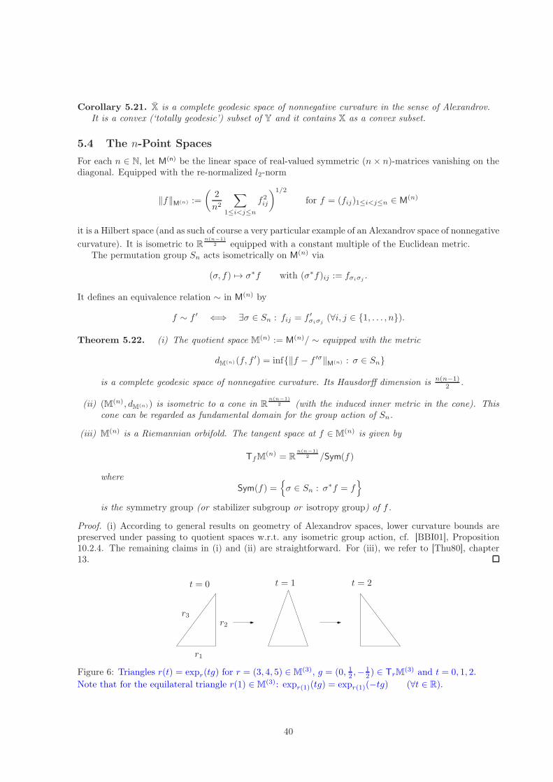
Corollary 5.21. X is a complete geodesic space of nonnegative curvature in the sense of Alexandrov.It is a convex (‘totally geodesic’) subset of Y and it contains X as a convex subset.

5.4 The n-Point Spaces

For each n ∈ N, let M(n) be the linear space of real-valued symmetric (n× n)-matrices vanishing on thediagonal. Equipped with the re-normalized l2-norm

‖f‖M(n) :=

(2

n2

∑

1≤i<j≤nf2ij

)1/2

for f = (fij)1≤i<j≤n ∈ M(n)

it is a Hilbert space (and as such of course a very particular example of an Alexandrov space of nonnegative

curvature). It is isometric to Rn(n−1)

2 equipped with a constant multiple of the Euclidean metric.The permutation group Sn acts isometrically on M(n) via

(σ, f) 7→ σ∗f with (σ∗f)ij := fσiσj .

It defines an equivalence relation ∼ in M(n) by

f ∼ f ′ ⇐⇒ ∃σ ∈ Sn : fij = f ′σiσj(∀i, j ∈ 1, . . . , n).

Theorem 5.22. (i) The quotient space M(n) := M(n)/ ∼ equipped with the metric

dM(n)(f, f ′) = inf‖f − f ′σ‖M(n) : σ ∈ Sn

is a complete geodesic space of nonnegative curvature. Its Hausdorff dimension is n(n−1)2 .

(ii) (M(n), dM(n)) is isometric to a cone in Rn(n−1)

2 (with the induced inner metric in the cone). Thiscone can be regarded as fundamental domain for the group action of Sn.

(iii) M(n) is a Riemannian orbifold. The tangent space at f ∈ M(n) is given by

TfM(n) = R

n(n−1)2 /Sym(f)

whereSym(f) =

σ ∈ Sn : σ∗f = f

is the symmetry group (or stabilizer subgroup or isotropy group) of f .

Proof. (i) According to general results on geometry of Alexandrov spaces, lower curvature bounds arepreserved under passing to quotient spaces w.r.t. any isometric group action, cf. [BBI01], Proposition10.2.4. The remaining claims in (i) and (ii) are straightforward. For (iii), we refer to [Thu80], chapter13.

r1

r2r3

t = 0 t = 1 t = 2

Figure 6: Triangles r(t) = expr(tg) for r = (3, 4, 5) ∈ M(3), g = (0, 12 ,− 12 ) ∈ TrM

(3) and t = 0, 1, 2.

Note that for the equilateral triangle r(1) ∈ M(3): expr(1)(tg) = expr(1)(−tg) (∀t ∈ R).

40

r1 r2

r3

Figure 7: For r = (1, 1, 2) and g = (0, 0, 1): g ∈ TrM(3) but g 6∈ TrM

(3)≤ .

Now let us consider the subset M(n)≤ in M(n) consisting of those symmetric (n×n)-matrices (fij)1≤i<j≤n

which ‘satisfy the triangle inequality’ in the following sense:

fij + fjk ≥ fik (∀i, j, k ∈ 1, . . . , n). (5.5)

Note that this constraint is compatible with the equivalence relation ∼ induced by the action of thepermutation group Sn:

∀f, f ′ ∈ M(n) with f ∼ f ′ : f ∈ M(n)≤ ⇐⇒ f ′ ∈ M

(n)≤ .

Hence, the space M(n)≤ := Mn

≤/ ∼ coincides with the subset of M(n) of equivalence classes of f whichsatisfy (5.5).

Example 5.23. The simplest non-trivial case is n = 3. Here

M(3) =

0 r1 r2r1 0 r3r2 r3 0

: r = (r1, r2, r3) ∈ R

3

andM

(3)≤ =

r ∈ R

3 : r1 ≤ r2 + r3, r2 ≤ r3 + r1, r3 ≤ r1 + r2

.

A fundamental domain of the quotient space M(3)/S3 is for instance given by

M(3) =r ∈ R

3 : r1 ≤ r2 ≤ r3

.

r2 r3

r1

(a) The domain bounded by the blue lines is

M(3)≤ ∩ S

2.

(b) The red colored area isM

(3)∩ S

2.

41

Figure 8: The green vectors illustrate elements in TfM(3)≤ which are mutually identified, whereas the

black vector is in TfM(3), but not in in TfM

(3)≤ .

Corollary 5.24. (i) M(n)≤ is a closed convex subset of M(n). It is itself an Alexandrov space of non-

negative curvature with dimension n(n−1)2 .

(ii) For f ∈ M(n)≤ the tangent space TfM

(n)≤ consists of those g ∈ TfM

(n) for which expf (tg) = f + tg

stays within M(n)≤ at least for some t > 0.

Now let us consider the injection

Φ :M(n) → Y,

f = (fij)1≤i<j≤n 7→ X = [[1, . . . , n, f, 1n

∑ni=1 δi]].

Elements in the image Y(n) := Φ(M(n)

)are called n-point spaces. They are characterized as gauged

measure spaces for which the mass is uniformly distributed on n (not necessarily distinct) points. Forconvenience, we also require that the gauge functions vanish on the diagonal. The image

X(n) := Φ

(M

(n)≤

)

of M(n)≤ consist of those mm-spaces with mass uniformly distributed on n points.

Proposition 5.25. For each n ∈ N, Φ is a 1-Lipschitz map:

∆∆(Φ(f),Φ(g)

)≤ dM(n)(f, g) (∀f, g ∈ M

(n)).

Moreover,size

(Φ(f)

)= ‖f‖M(n).

Proof. Obviously, size2(Φ(f)

)= 1

n2

∑ni,j=1 f

2ij = ‖f‖2

M(n). Moreover, (cf. Proposition 4.1)

−∆∆2(Φ(f),Φ(g)

)+ size2

(Φ(f)

)+ size2

(Φ(g)

)= sup

p∈P(n)

2

n2

n∑

i,j=1

n∑

k,l=1

fij · gkl · pik · pjl

where P(n) denotes the set of doubly stochastic (n× n)-matrices, i.e. set of all p = (pij)1≤i,j≤n ∈ Rn×n+

satisfying∑n

i=1 pil =∑n

j=1 pkj = 1 for all k, l = 1, . . . , n. Particular examples of such doubly stochasticmatrices are given for each σ ∈ Sn by

pij = δiσj .

42

The claim thus follows from the fact that

−d2M(n)

(f, g)+ ‖f‖2

M(n) + ‖g‖2M(n) = sup

σ∈Sn

2

n2

n∑

i,j=1

fij · gσiσj .

Remark 5.26. The injection

Φ : M(n)≤ → X

is an embedding. Indeed, assume that

∆∆(Φ(dk),Φ(d∞)

)→ 0 as k → ∞

for some d∞ ∈ M(n)≤ and some sequence (dk)k∈N in M

(n)≤ . Assume for simplicity that d∞ and all the dk

are metrics on 1, . . . , n. (All d∞, dk ∈ M(n)≤ can be approximated by metrics.) The dk are uniformly

bounded. Thus according to Corollary 2.10

D2

(Φ(dk),Φ(d∞)

)→ 0 as k → ∞.

According to the union lemma ([Gro99], [Stu06]) this implies that there exists a metric space (X, d) andisometric embeddings ηk :

(1, . . . , n, dk

)→ (X, d) for all k ∈ N ∪ ∞ such that

d2

((ηk)∗

( 1n

n∑

i=1

δi), (η∞)∗

( 1n

n∑

j=1

δj))

→ 0 as k → ∞

where d2 now denotes the L2-Wasserstein distance for probability measures on (X, d), i.e.

d2

((ηk)∗

( 1n

n∑

i=1

δi), (η∞)∗

( 1n

n∑

j=1

δj))

= inf 1

n

n∑

i,j=1

d2(ηk(i), η∞(j)

)pij :

∑

l

pil =∑

l

plj = 1 for all i, j1/2

.

For this ‘classical’ transport problem, however, it is known that the infimum is attained (among others)on the set of extremal points within the set of doubly stochastic matrices. Hence,

d2

((ηk)∗

( 1n

n∑

i=1

δi), (η∞)∗

( 1n

n∑

j=1

δj))

= inf 1

n

n∑

i=1

d2(ηk(i), η∞(σi)

): σ ∈ Sn

1/2

.

Moreover, the triangle inequality for d implies

2 inf 1

n

n∑

i=1

d2(ηk(i), η∞(σi)

): σ ∈ Sn

1/2

≥ inf 1

n2

n∑

i,j=1

∣∣∣d(ηk(i), ηk(j)

)− d(η∞(σj), η

∞(σi))∣∣∣

2

: σ ∈ Sn

1/2

= inf 1

n2

n∑

i,j=1

∣∣∣dkij − d∞σjσi

∣∣∣2

: σ ∈ Sn

1/2

= dM(n)

(dk, d∞

).

This finally implies dM(n)

(dk, d∞

)→ 0 as k → ∞ which is the claim.

Challenge 5.27. Prove or disprove that the injections

Φ : M(n) → Y

andΦ : M

(n)≤ → X

are isometric embeddings.

43

Proposition 5.28.⋃

n∈N X(n) is dense in X and⋃

n∈N Y(n) is dense in Y.

Proof. The density assertion (w.r.t. ∆∆) concerning X or X is an immediate consequence of the analogousdensity statement for X w.r.t. D in [Stu06], Lemma 3.5, and the estimate ∆∆ ≤ 2D of Lemma 2.6.

To see the density assertion concerning Y, let a gauged measure space X be given. We alwayscan choose a representative (X, f,m) without atoms. The gauge function f ∈ L2

s(X2,m2) then can be

approximated in L2-norm by piecewise constant functions f(n) ∈ L2s(X

2,m2), n ∈ N. Even more, these

functions f(n) on X ×X can be chosen to be constant on X(n)i ×X

(n)j for 1 ≤ i < j ≤ n for a suitable

partition of X into sets X(n)i of volume 1

n (∀i = 1, . . . , n). That is, for each n ∈ N the gauged measure

space (X, f(n),m) is homomorphic to the n-point space(1, . . . , n, f (n), 1

n

∑ni=1 δi

)for

f(n)ij := f(n)

∣∣∣X

(n)i ×X(n)

j

(∀1 ≤ i < j ≤ n).

The spaces M(n) also play a key role in the ‘reconstruction theorem’ of Gromov [Gro99] and Vershik[Ver98] based on ‘random matrix distributions’. For each n ∈ N and each gauged measure space (X, f,m),

let ν(X,f,m)n denote the distribution of the matrix

(f(xi, xj)

)1≤i<j≤n ∈ M(n)

under the measure dmn(x1, . . . , xn). Here mn = m⊗n denotes the n-fold product measure of m. Letm∞ = m⊗N denote the infinite product of m defined on X∞ = (xi)i∈N : xi ∈ X, put

M(∞) =(fij)1≤i<j<∞ : fij ∈ R

and let ν(X,f,m)∞ denote the distribution of

(f(xi, xj)

)1≤i<j<∞ ∈ M(∞)

under the measure dm∞(x1, x2, . . .).

Proposition 5.29. For the following assertions, the implications (i) ⇒ (ii) ⇔ (iii) hold true for allgauged measure spaces (X, f,m) and (X ′, f′,m′):

(i) (X, f,m) and (X ′, f′,m′) are homomorphic (as elements in Y)

(ii) For each n ∈ N: ν(X,f,m)n and ν

(X′,f′,m′)n coincide (as probability measures on M(n))

(iii) ν(X,f,m)∞ and ν

(X′,f′,m′)∞ coincide (as probability measures on M(∞)).

For metric measure spaces (X, f,m) and (X ′, f′,m′), the assertions (i), (ii) and (iii) are equivalent.

Proof. (i) ⇒ (ii) Assuming the spaces to be homomorphic amounts to assume that there exists a measurem ∈ Cpl(m,m′) on X ×X ′ such that f(x, y) = f′(x′, y′) for m2-a.e. ((x, x′), (y, y′)). Thus

distr. of(f(xi, xj)

)1≤i<j≤n

under dmn(x1, . . . , xn

)

= distr. of(f(xi, xj)

)1≤i<j≤n

under dmn((x1, x

′1), . . . , (xn, x

′n))

= distr. of(f′(x′i, x

′j))1≤i<j≤n

under dmn((x1, x

′1), . . . , (xn, x

′n))

= distr. of(f′(x′i, x

′j))1≤i<j≤n

under dm′n(x′1, . . . , x

′n

).

(ii) ⇔ (iii): Straightforward consequence of the fact that the Borel field in M(∞) is generated by pre-images under projections into M(n), n ∈ N.

(iii) ⇒ (i): Reconstruction theorem [Gro99], 3 12 .5.

44

6 The Space Y as a Riemannian Orbifold

6.1 The Symmetry Group

Let Polish spaces X1, X2, X3 with Borel probability measures m1,m2,m3 be given as well as couplingsµ′ ∈ Cpl(m1,m2) and µ′′ ∈ Cpl(m2,m3). Recall the gluing construction from Lemma 1.4 which yields ameasure µ = µ′ ⊠ µ′′ on X1 ×X2 ×X3 with (π1, π2)∗µ = µ′ and (π2, π3)∗µ = µ′′.

Definition 6.1. The melting of µ′ and µ′′ is the probability measure µ ∈ Cpl(m1,m3) defined as

µ = (π1, π3)∗(µ′⊠ µ′′).

It will be denoted by µ′ ⊡ µ′′.

Lemma 6.2. Let a gauged measure space (X, f,m) be given.

(i) Cpl(m,m), the space of all self-couplings of m, is a group with composition ⊡. The neutral elementis the diagonal coupling

dν(x, y) = dδx(y) dm(x).

The element inverse to µ is given by

dµ−1(x, y) = dµ(y, x).

(ii) A norm is given on this group by

‖µ‖f =

(∫

X

∫

X

∣∣∣f(x0, y0)− f(x1, y1)∣∣∣2

dµ(x0, x1) dµ(y0, y1)

)1/2

.

Proof. (i) is obvious: the gluing of µ and µ−1 for instance is given by (π1, π2, π1)∗µ. Projecting this ontothe first and third factor yields

(π1, π1)∗µ = (π1, π1)∗m

which is the diagonal coupling.(ii) The inequality to be verified

‖µ′ ⊡ µ′′‖f ≤ ‖µ′‖f + ‖µ′′‖f

follows exactly in the same way as the triangle inequality for ∆∆.

Definition 6.3. The symmetry group of (X, f,m) is the subgroup of Cpl(m,m) of elements with vanishingnorm:

Sym(X, f,m) =µ ∈ Cpl(m,m) : ‖µ‖f = 0

.

In other words, Sym(X, f,m) is the set of all optimal couplings of (X, f,m) with itself.We say, that (X, f,m) has no symmetries if Sym(X, f,m) only contains the neutral element (diagonal

coupling).

The symmetry group Sym(X, f,m) will depend on the choice of the representative within the equiva-lence class [[X, f,m]]. For different choices of representatives, the groups will be obtained from each othervia conjugation and thus in particular will be isomorphic to each other.

Lemma 6.4. Let two homomorphic gauged measure spaces (X, f,m) and (X ′, f′,m′) be given with ν ∈Opt(m,m′) being a coupling which realizes the vanishing ∆∆-distance. Then

Sym(X ′, f′,m′) = ν−1 ⊡ Sym(X, f,m) ⊡ ν

=µ′ = ν−1 ⊡ µ⊡ ν : µ ∈ Sym(X, f,m)

.

45

Proof. The fact that µ is in Sym(X, f,m) implies that f(x0, y0) = f(x1, y1) for µ2-a.e. ((x0, x1), (y0, y1)) ∈X2 × X2. The fact that ν realizes the (vanishing) distance of (X, f,m) and (X ′, f′,m′) implies thatf(x0, y0) = f′(x′0, y

′0) for ν2-a.e. ((x0, x

′0), (y0, y

′0)) ∈ (X ×X ′)2. Thus

f′(x′0, y′0) = f(x0, y0) = f(x1, y1) = f′(x′1, y

′1)

for (ν−1 ⊠ µ ⊠ ν)2-a.e. ((x′0, x0, x1, x′1), (y

′0, y0, y1, y

′1)) ∈ (X ′ ×X × X ×X ′)2. Projecting the measure

ν−1 ⊠ µ⊠ ν from X ′ ×X ×X ×X ′ onto X ′ ×X ′ yields the claim:

f′(x′0, y′0) = f′(x′1, y

′1)

for (ν−1 ⊡ µ⊡ ν)2-a.e. ((x′0, x′1), (y

′0, y′1)) ∈ (X ′ ×X ′)2.

If the underlying space is not just a gauged measure space but a metric measure space, then thesymmetry group admits an equivalent representation in more familiar terms.

Definition 6.5. Given a metric measure space (X, d,m), let

sym(X, d,m) =φ : X → X : m = φ∗m, d = φ∗d

where X denotes the support of m.

Note that any φ which preserves the metric is Lipschitz continuous and thus in particular Borelmeasurable. If moreover it is measure preserving, then according to the proof of (iii) ⇒ (iv) in Lemma1.10 it is necessarily bijective with Borel measurable inverse.

Lemma 6.6. Let (X, d,m) be a metric measure space.

(i) sym(X, d,m) is a group (with composition of maps as group operation)

(ii) The groups sym(X, d,m) and Sym(X, d,m) are isomorphic. For any φ ∈ sym(X, d,m) the corre-sponding measure in µ ∈ Sym(X, d,m) is given by

µ := (Id, φ)∗m.

(iii) Let (X ′, d′,m′) be another metric measure space, isomorphic to the first one with ψ : X → X ′

being a Borel measurable bijection which pushes forward the measure and pulls back the metric.Then

sym(X ′, d′,m′) = ψ sym(X, d,m) ψ−1.

Proof. Most properties are obvious. Let us briefly comment on the inverse of the isomorphism in (ii).Let a measure µ ∈ Sym(X, d,m) be given. It is an optimal coupling of (X, d,m) with itself with vanishing∫ ∫

|d − d|2dµdµ. According to Lemma 1.10 this implies that there exists a bijective Borel map (withBorel inverse) φ : X → X satisfying m = φ∗m and d = φ∗d.

6.2 Geodesic Hinges

A geodesic hinge is a pair of geodesics (Xt)0≤t≤τ and (X ′t )0≤t≤τ ′ emanating from a common point X0 = X ′0in Y. To simplify the presentation, we assume τ = τ ′ = 1. (Since the geodesics are not required to haveunit speed, this is no restriction.)

We fix representatives (X0, f0,m0), (X1, f1,m1) and (X ′1, f′1,m

′1) of the endpoints as well as optimal

couplings m ∈ Cpl(m0,m1) and m′ ∈ Cpl(m0,m′1). We are now looking for couplings of m and m′, that

is, for µ ∈ Cpl(m, m′) being measures on X = X0 ×X1 ×X0 ×X ′1. The projections onto the respectivefactors will be denoted by π0, π1, π

′0, π′1. Note that the factor X0 shows up twice in the definition of µ.

For t ∈ (0, 1], we define the functional

Ct(µ) =1

t2

∫

X

∫

X

∣∣∣∣(1 − t)[f0(x0, y0)− f0(x

′0, y′0)]

+t[f1(x1, y1)− f′1(x

′1, y′1)]∣∣∣∣

2

dµ(x0, x1, x′0, x′1) dµ(y0, y1, y

′0, y′1)

46

on Cpl(m, m′). Moreover, we put

C0(µ) = supt>0

Ct(µ).

Lemma 6.7. (i) For each t ∈ (0, 1], there exists a measure µt ∈ Cpl(m, m′) which minimizes Ct(.), an’optimal’ coupling of m and m

′ w.r.t. the cost function |ft − f′t|2.

(ii) The quantity

C∗t = Ct(µt) =1

t2∆∆2(Xt,X ′t )

is non-increasing in t.

(iii) For each µ with(π0, π

′0

)∗µ ∈ Sym(X0, f0,m0),

t 7→ Ct(µ) is independent of t ∈ (0, 1]

and thus C0(µ) = Ct(µ) = C1(µ). In particular,

C0(µ) =

∫

X

∫

X

[f1(x1, y1)− f′1(x

′1, y′1)]2dµ(x0, x1, x

′0, x′1) dµ(y0, y1, y

′0, y′1) <∞.

(iv) For each µ with(π0, π

′0

)∗µ 6∈ Sym(X0, f0,m0),

C0(µ) = ∞.

(v) The functional C0 is lower semicontinuous on Cpl(m, m′).

(vi) Every accumulation point µ0 of (µt)t>0 satisfies(π0, π

′0

)∗µ0 ∈ Sym(X0, f0,m0).

Proof. (i) follows from the existence result in Proposition 5.4 and the fact that

C∗t = infCt(µ) : µ ∈ Cpl(m, m′)

=

1

t2∆∆2(Xt,X ′t ).

(ii) is a general consequence of nonnegative curvature in Alexandrov geometry.(iii), (iv) are obvious: If the condition

(π0, π

′0

)∗µ ∈ Sym(X0, f0,m0) was not satisfied then obviously

C0(µ) = ∞. On the other hand, the previously mentioned condition(π0, π

′0

)∗µ ∈ Sym(X0, f0,m0) implies

Ct(µ) = C1(µ) <∞ independent of t and thus C0(µ) = C1(µ) <∞.(v) According to Lemma 5.3, we may assume without restriction that X0 = X1 = X ′1 = I and

m0 = m1 = m′1 = L1. With the same argument as in the proof of Lemma 5.5 (approximating f0, f1, f′1 ∈ L2

by bounded continuous f0,i, f1,i, f′1,i), Ct(.) is proven to be continuous on Cpl(m, m′). As a supremum of

continuous functionals Ct, the functional C0 is lower semicontinuous.(vi) Assume that

(π0, π

′0

)∗µ0 6∈ Sym(X0, f0,m0) for an accumulation point µ0 of the family (µt)t>0.

Then ∫

X

∫

X

[f0(x0, y0)− f0(x

′0, y′0)]2dµ0(x0, x1, x

′0, x′1) dµ0(y0, y1, y

′0, y′1) ≥ 2ǫ > 0

and thus for a converging (sub)sequence (µtn)n,

∫

X

∫

X

[f0(x0, y0)− f0(x

′0, y′0)]2dµtn(x0, x1, x

′0, x′1) dµtn(y0, y1, y

′0, y′1) ≥ ǫ

uniformly in n. This impliesCtn(µtn) ր ∞

which contradicts the minimality of µtn .

Proposition 6.8. Let a geodesic hinge (Xt)0≤t≤1 and (X ′t )0≤t≤1 be given as above with speeds R =∆∆(X0,X1), R

′ = ∆∆(X0,X ′1) and representatives (X0×X1, f0+ t(f1− f0), m), (X0×X ′1, f0+ t(f′1− f0), m′),

resp. Then there exists a probability measure µ on X := X0 ×X1 ×X0 ×X ′1 with

47

• µ ∈ Cpl(m, m′), more precisely, (π0, π1)∗µ = m and (π′0, π′1)∗µ = m′

• (π0, π′0)∗µ ∈ Sym(X0, f0,m0)

and

C0(µ) = infC0(µ) : µ ∈ Cpl(m, m′), (π0, π

′0)∗µ ∈ Sym(X0, f0,m0)

.

Equivalently,

⟨f1 − f0, f

′1 − f0

⟩L2(X2,µ2)

= sup⟨

f1 − f0, f′1 − f0

⟩L2(X2,µ2)

: µ ∈ Cpl(m, m′),

(π0, π′0)∗µ ∈ Sym(X0, f0,m0)

.

Moreover,

cos∡(X•,X ′•

)≥ 1

RR′⟨f1 − f0, f

′1 − f0

⟩L2(X2,µ2)

.

Proof. The existence of µ follows from the lower semicontinuity of C0 proven in the previous Lemma.Moreover,

C0(µ) = limt→0

Ct(µ) ≥ limt→0

C∗t .

On the other hand, nonnegative curvature of Y implies that the angle between the geodesics always exists.Indeed, it is a monotone limit

cos∡(X•,X ′•

)= lim

t→0

1

2RR′

[R2 +R′2 − 1

t2∆∆(Xt,X ′t )

]

=1

2RR′

[R2 +R′2 − lim

t→0C∗t

].

Finally, since f0(x0, y0) = f0(x′0, y′0) for µ2-a.e.

((x0, x1, x

′0, x′1), (y0, y1, y

′0, y′1))∈ X2 we may rewrite the

previous expressions for each coupling µ (with the required properties of its pairwise marginals) as follows

R2 +R′2 − C0(µ)

=

∫

X

∫

X

([f1(x1, y1)− f0(x0, y0)

]2+[f′1(x

′1, y′1)− f0(x

′0, y′0)]2

−[f1(x1, y1)− f′1(x

′1, y′1)]2)

dµ(x0, x1, x′0, x′1) dµ(y0, y1, y

′0, y′1)

= 2

∫

X

∫

X

[f1(x1, y1)− f0(x0, y0)

]·[f′1(x

′1, y′1)− f0(x

′0, y′0)]dµ(x0, x1, x

′0, x′1) dµ(y0, y1, y

′0, y′1).

This is the claim.

Conjecture 6.9. For each geodesic hinge as above,

cos∡(X•,X ′•

)=

1

RR′⟨f1 − f0, f

′1 − f0

⟩L2(X2,µ2)

.

6.3 Tangent Spaces and Tangent Cones

Definition 6.10. The tangent space at X ∈ Y is defined as

TX =⋃

[[X,f,m]]=XL2s(X

2,m2)/ ∼

with union taken over all gauged measure spaces (X, f,m) in the homomorphism class [[X, f,m]]. Hereg ∈ L2

s(X2,m2) and g′ ∈ L2

s(X′2,m′2) are regarded as equivalent, briefly g ∼ g′, if they are defined on

48

two representatives (X, f,m) and (X ′, f′,m′) of X for which there exists a coupling µ ∈ Cpl(m,m′) suchthat f = f′ and g = g′ µ2-a.e. on (X ×X ′)2. More precisely, the latter means that

f(x, y) = f′(x′, y′) and g(x, y) = g′(x′, y′)

for µ2-a.e.((x, x′), (y, y′)

)∈ (X ×X ′)2.

Remarks 6.11. (i) This, indeed, is an equivalence relation: g ∼ g′ and g′ ∼ g′′ implies g ∼ g′′.

(ii) For g, h defined as symmetric L2-functions on the same representative (X, f,m) of X , the aboveequivalence means that g = h µ2-a.e. for some µ ∈ Sym(X, f,m).

(iii) Given a gauged measure space (X, f,m), a probability space (X ′,m′) (for consistence, with X ′ beinga Polish space) is called “enlargement” of (X,m) if there exists a measurable map φ : X ′ → X withm = φ∗m′. In this case, the map

Φ : g 7→ φ∗g

defines an isometric embedding of the Hilbert space L2s(X

2,m2) into the Hilbert space L2s(X

′2,m′2).Put f′ = φ∗f. Then

g ∼ φ∗g

for each g ∈ L2s(X

2,m2). Indeed, µ := (φ, Id)∗m′ defines a coupling of m and m′ with the propertyf = f′, g = φ∗g µ2-a.e.

Therefore, for all g, h ∈ L2s(X

2,m2),

g ∼ h ⇐⇒ φ∗g ∼ φ∗h.

(iv) For each gauged measure space (X, f,m), the “standard” space (I,L1) together with some parametriza-tion φ ∈ Par(m) can be regarded as an enlargement. Hence, each tangent vector admits a represen-tative in L2

s(I2,L2). In other words, the tangent space can be considered as subspace of L2

s(I2,L2),

see section 6.4 below.

Definition 6.12. A metric dTX will be defined on the tangent space TX as follows: for g, h ∈ TX , sayg ∈ L2

s(X2,m2), h ∈ L2

s(X′2,m′2) with [[X, f,m]] = [[X ′, f′,m′]] = X , we put

dTX (g, h) = inf‖g − h‖L2((X×X′)2,µ2) : µ ∈ Cpl(m,m′), f = f′ µ2-a.e. on (X ×X ′)2

.

Remarks 6.13. (i) dTX is symmetric and satisfies the triangle inequality.

(ii) dTX (g, h) = 0 if and only if g ∼ h.

(iii) Given g, h ∈ TX , say g ∈ L2s(X

2,m2), h ∈ L2s(X

′2,m′2) with [[X, f,m]] = [[X ′, f′,m′]] = X , choosea common enlargement (X, m) of (X,m) and (X ′,m′) with embeddings φ : X → X , φ′ : X → X ′.Since the spaces (X, f,m) and (X ′, f′,m′) are homomorphic we may assume without restriction thatφ∗f = φ′∗f′ =: f. Put g = φ∗g, h = φ∗h. Then g ∼ g, h ∼ h and

dTX (g, h) = dTX (g, h) = inf‖g − h‖L2(X4,µ2) : µ ∈ Sym(X, f, m)

.

Lemma 6.14. dTX is a cone metric on TX .

Proof. The claim will follow from the fact that for each g ∈ L2s(X

2,m2), h ∈ L2s(X

′2,m′2) with ‖g‖L2 =‖h‖L2 = 1, the quantity

1

2st

[dTX (sg, th)

2 − s2 − t2]

is independent of s and t ∈ (0,∞). The latter can be seen as follows

1

2st

[dTX (sg, th)

2 − s2 − t2]

= inf 1

2st

[‖sg − th‖2L2((X×X′)2,µ2) − s2 − t2

]: µ ∈ Cpl(m,m′), f = f′ µ2-a.e.

= − sup〈g, h〉L2((X×X′)2,µ2) : µ ∈ Cpl(m,m′), f = f′ µ2-a.e.

.

49

Definition 6.15. The exponential map ExpX : TX → Y is defined by

g 7→ [[X, f + g,m]]

for g ∈ L2s(X

2,m2).

Remark 6.16. This definition is consistent since g ∼ g′ implies [[X, f + g,m]] = [[X ′, f′ + g′,m′]]. Indeed,given g ∈ L2

s(X2,m2), g′ ∈ L2

s(X′2,m′2) with [[X, f,m]] = [[X ′, f′,m′]], we know that g ∼ g′ if and only if

there exists a measure µ ∈ Cpl(m,m′) such that f = f′ and g = g′ µ2-a.e. This implies f + tg = f′ + tg′

µ2-a.e. for every t ∈ R which in turn implies

[[X, f + tg,m]] = [[X ′, f′ + tg′,m′]]

for every t ∈ R. In other words,ExpX (tg) = ExpX (tg

′)

for every t. Thus Exp is well-defined.

Definition 6.17. For X ∈ Y we define the map τYX : TX → [0,∞] by

τYX (g) = supt ≥ 0 :

(ExpX (sg)

)s∈[0,t] is geodesic in Y

.

Analogously, for X ∈ X, we define

τ XX (g) = supt ≥ 0 :

(ExpX (sg)

)s∈[0,t] is geodesic in X

.

Recall that TXY, the tangent cone at X in the sense of Alexandrov geometry (cf. section 4.3.), isdefined as the cone over its unit sphere T 1

XY which in turn is the completion of the space of geodesic

directions T 1XY. Equivalently, TXY can be considered as the completion of TXY which in turn is the cone

over T 1XY. Denote the metric on TXY by dYX .

Theorem 6.18. (i) The setg ∈ TX : τYX (g) > 0

can be identified with the cone TXY via g 7→(

ExpX (sg))s∈[0,τY

X(g))

.

(ii) For each g ∈ TX , say g ∈ L2s(X

2,m2), with τYX (g) > 0,

dYX (g, 0) = ‖g‖TXY = ‖g‖L2(X2,m2) = dTX (g, 0).

(iii) For all g, h ∈ TXY,dYX (g, h) ≤ dTX (g, h).

Proof. (i),(ii) By definition, for each g ∈ TX with τYX (g) > 0,(ExpX (sg)

)s∈[0,τY

X(g))

is a geodesic in

Y. Hence, g is an element of the cone TXY. Conversely, each geodesic (Xs)s∈[0,t] in Y emanating fromX = X0 can be represented as Xs = ExpX (sg) for suitable g ∈ L2

s(X2,m2) and suitable representative

(X, f,m) of X .(iii) To prove the inequality between the distances on TXY and TX it suffices to verify the analogous

inequality between the induced distances on the respective unit spheres T 1XY and T

1X (since both spaces

are cones over their respective unit spheres). Let representatives (X, f,m) and (X ′, f′,m′) of X be givenas well as unit tangent vectors g ∈ L2

s(X2,m2) and g′ ∈ L2

s(X′2,m′2). Then

dY,1X (g, g′) = ∡

((ExpX (sg)

)s≥0,

(ExpX (tg

′))t≥0

)

whereascos dT,1X (g, g′) = sup

〈g, g′〉L2((X×X′)2,µ2) : µ ∈ Cpl(m,m′), f = f′ µ2-a.e.

According to Proposition 6.8 (with f, f′ in the place of f0, f0 and g, g′ in the place of f1 − f0, f′1 − f0)

cos dT,1X (g, g′) ≤ cos dY,1X (g, g′).

This proves the claim.

50

Corollary 6.19. (i) The setg ∈ TX : τ XX (g) > 0

can be identified with the cone TX X.

(ii) For all g, h ∈ TX X ⊂ TXY,

dXX (g, h) = dYX (g, h) ≤ dTX (g, h).

6.4 Tangent Spaces – A Comprehensive Alternative Approach

Recall the fact (sect. 5.2) that the space Y of gauged measure space is isometric to a quotient space L ofL2s(I

2,L2). The tangent spaces TX for X = [[X, f,m]] ∈ Y, therefore, will be in one-to-one correspondencewith the tangent spaces Tf (to be defined below) for f ∈ L.

Given a function f ∈ L2s(I

2,L2), we put

Sym(f) =(ψ0, ψ1) ∈ Inv(I,L1)2 : ψ∗0 f = ψ∗1 f

.

Note that this will be a group, isomorphic to the previously introduced Sym(I, f,L1), provided we identifyall (ψ0, ψ1) ∈ Sym(f) which satisfy ψ0 = ψ1. (The latter should be understood as identity L2-a.e. asusual.) We say that f has no symmetries if

∀ψ0, ψ1 ∈ Inv(I,L1) : ψ∗0 f = ψ∗1 f =⇒ ψ0 = ψ1.

Definition 6.20. The tangent space

Tf = L2s(I

2,L2)/ Sym(f)

is the quotient space of L2s(I

2,L2) with respect to the equivalence relation

g ∼ h ⇐⇒ ∃(ψ0, ψ1) ∈ Sym(f) : ψ∗0g = ψ∗1h.

It is a metric space with metric

df(g, h) = inf‖ψ∗0g − ψ∗1h‖L2(I2,L2) : (ψ0, ψ1) ∈ Sym(f)

.

If f has no symmetries then Tf = L2s(I

2,L2). In particular, then Tf is a Hilbert space.

This definition justifies to regard the tangent spaces Tf (and thus also the previously defined tangentspaces TX ) as infinite dimensional Riemannian orbifolds.

Definition 6.21. The exponential map Expf : Tf → L is defined by

g 7→ [[f + g]].

Equivalently, it may be considered as map Expf : Tf → Y with

g 7→ [[I, f + g,L1]].

Indeed, however, the measure space (I,L1) does not play any particular role. It is just one of manypossible enlargements of a given space. It can be replaced by any other standard Borel space withoutatoms. Thus for any gauged measure space (X, f,m) without atoms we may define

T(X,f,m) = L2s(X

2,m2)/Sym(X, f,m)

where two elements g and h in L2s(X

2,m2) are identified if there exists a measure µ ∈ Sym(X, f,m) – aself-coupling of m which leaves f invariant – such that

g(x, y) = h(x′, y′) for µ2-a.e.((x, x′), (y, y′)

)∈ X4.

For g ∈ T(X,f,m) we putExp(X,f,m)(g) = [[X, f + g,m]].

Corollary 6.22. For each gauged measure space (X, f,m) without atoms, the space T(X,f,m) may be iden-tified with the tangent space TX where X denotes the homomorphism class of (X, f,m). The exponentialmaps Exp(X,f,m) and ExpX are defined consistently.

51

6.5 Ambient Gradients

Definition 6.23. A function U : Y → R is called strongly differentiable at X ∈ Y

• if the directional derivative

DhU(X ) := limtց0

1

t

[U(ExpX (th))− U(X )

]

exists for every h ∈ TX and

• if there exists a tangent vector g ∈ TX such that

DhU(X ) = 〈g, h〉L2((X×X′)2,µ2)

for every h ∈ TX and every µ ∈ Cpl(m,m′) with f = f′ µ2-a.e. on (X ×X ′)2.

Here we assumed g ∈ L2s(X

2,m2) and h ∈ L2s(X

′2,m′2) with (X, f,m) and (X ′, f′,m′) being tworepresentatives of X .

The tangent vector g ∈ TX is then called ambient gradient of U at X . It is denoted by

g = ∇∇U(X ).

Lemma 6.24. For any function U : Y → R which is strongly differentiable at X ∈ Y, the ambientgradient is unique and satisfies

‖∇∇U(X )‖ = supDhU(X ) : ‖h‖ = 1

.

Here ‖h‖ = ‖h‖L2(X′2,m′2) = dTX (h, 0) for h ∈ L2s(X

′2,m′2) and ‖g‖ = ‖g‖L2(X2,m2) = dTX (g, 0) forg = ∇∇U(X ) ∈ L2

s(X2,m2) with representatives (X, f,m) and (X ′, f′,m′) of X .

Proof. Uniqueness. In order to be the ambient gradient ∇∇U(X ), a function g ∈ L2s(X

2,m2) in particularhas to satisfy

DhU(X ) = 〈g, h〉L2(X2,µ2) for every h ∈ L2s(X

2,m2).

(Indeed, choose X ′ = X and µ to be diagonal coupling.) The latter property determines g (if it exists)uniquely within L2

s(X2,m2). Two ambient gradients g and g′ defined on two representatives of X may

always be extended (via pull back) to functions on a common enlargement. Thus the ambient gradientis unique (if it exists).

Norm identity. For each h and each coupling µ (which leaves f invariant) as above

DhU(X ) = 〈g, h〉L2((X×X′)2,µ2)

≤ ‖g‖L2((X×X′)2,µ2) · ‖h‖L2((X×X′)2,µ2)

= ‖g‖L2(X2,m2) · ‖h‖L2(X′2,m′2).

Thus DhU(X ) ≤ ‖g‖ for each h ∈ TX with ‖h‖ = 1. On the other hand, assume without restriction that‖g‖ > 0 and choose h = 1

‖g‖g and µ = diagonal coupling of m to obtain

DhU(X ) =1

‖g‖〈g, g〉L2((X×X)2,µ2) = ‖g‖.

Theorem 6.25. Let U : Y → R be Lipschitz continuous, semiconcave and strongly differentiable inX ∈ Y. Assume that the ambient gradient ∇∇U(X ) lies in TXY or, in other words, assume that τYX (g) > 0for g = ∇∇U(X ). Then

∇∇U(X ) = ∇YU(X ).

Here ∇Y denotes the gradient in the sense of Alexandrov geometry as introduced e.g. in section 4.3, see[Pla02].

52

Proof. Put g = ∇∇U(X ). According to the argumentation in the proof of the previous Lemma, g1 = 1‖g‖g

is the maximizer ofh 7→ DhU(X )

in T1X . Therefore, assuming that g ∈ TXY, the normalized g1 in particular is the maximizer of h 7→

DhU(X ) in T 1XY. Up to a multiplicative constant, this already characterizes the gradient of U at X in

the sense of Alexandrov geometry. The previous Lemma finally yields the equivalence of the norms (=lengths of tangent vectors) in both spaces.

Corollary 6.26. Let U : Y → R be defined on all of Y and assume that its restriction to X is Lipschitzcontinuous and semiconcave. Assume furthermore that U is strongly differentiable in X ∈ X and that theambient gradient ∇∇U(X ) lies in TX X. Then

∇∇U(X ) = ∇XU(X ).

7 Semiconvex Functions on Y and their Gradients

7.1 Polynomials on Y and their Derivatives

A striking consequence of the detailed knowledge of the geometry of Y is that for major classes of functionson Y one can explicitly calculate sharp bounds for derivatives of any order. Of particular interest will bebounds for first and second derivatives.

An important class of ‘smooth’ functions on Y is given by polynomials of order n ∈ N. These arefunctions U : Y → R of the form

U(X ) =

∫

Xn

u

((d(xi, xj)

)1≤i<j≤n

)dmn(x) (7.1)

for X = [[X, d,m]] where u : Rn(n−1)

2 → R is any Borel function which grows at most quadratically.Mostly, u will be differentiable with bounded derivatives of any order. For our purpose, derivatives oforder 1 and 2 are sufficient. Here and in the sequel, mn = m ⊗ . . .⊗ m denotes the n-fold product of m

and x = (x1, . . . , xn) ∈ Xn whereas ξ = (ξij)1≤i<j≤n ∈ Rn(n−1)

2 . Deviating from the convention of theprevious Chapter, the gauge function will be denoted by d. In most cases of application, indeed, it willbe a pseudo metric.

Note that all these functions U are functions of homomorphism classes, i.e. the definition of U(X )does not depend on the choice of the representative (X, d,m) of X , see Proposition 5.29. Moreover, itmight be worthwhile to mention that the set of polynomials of any order separates points in X ([Gro99],cf. also [GPW09], Prop. 2.6)

Recall that each geodesic (Xt)0≤t≤1 in Y can be represented as

Xt = [[X0 ×X1, d0 + t(d1 − d0), m]] (7.2)

for given representatives of X0 and X1 and a suitable choice of m ∈ Opt(m0,m1). Thus U is representedalong the geodesic (Xt)0≤t≤1 as

U(Xt

)=

∫

(X0×X1)nu

((d0(x

i0, x

j0) + t

(d1(x

i1, x

j1)− d0(x

i0, x

j0)))

1≤i<j≤n

)dmn(x0, x1) (7.3)

where (x0, x1) now stands for the n-tuple ((xi0, xi1))1≤i≤n of points (xi0, x

i1) ∈ X0 ×X1.

Lemma 7.1. Assume that U : Y → R is given by formula (7.1) with u ∈ C2(Rn(n−1)

2 ,R+) with boundedderivatives. Then for each geodesic (Xt)0≤t≤1 in Y (represented as in (7.2)):

d

dtU(Xt) =

∑

1≤i<j≤n

∫

(X0×X1)n

∂

∂ξiju

((d0(x

p0 , x

q0) + t

(d1(x

p1, x

q1)− d0(x

p0, x

q0)))

1≤p<q≤n

)·

·(d1(x

i1, x

j1)− d0(x

i0, x

j0)

)dmn(x0, x1)

53

and

d2

dt2U(Xt) =

∑

1≤k<l≤n

∑

1≤i<j≤n

∫

(X0×X1)n

∂

∂ξkl

∂

∂ξiju

((d0(x

p0, x

q0) + t

(d1(x

p1, x

q1)− d0(x

p0, x

q0)))

1≤p<q≤n

)·

·(d1(x

i1, x

j1)− d0(x

i0, x

j0)

)·(d1(x

k1 , x

l1)− d0(x

k0 , x

l0)

)dmn(x0, x1)

for all t ∈ (0, 1) and as a right limit for t = 0.

Proof. These formulae are straightforward consequences of the representation of (7.3): interchangingorder of differentiation (w.r.t. t) and integration (w.r.t. xi0, x

i1) and application of chain rule.

Note that at t = 0 the previous formulas simplify, e.g.

d

dtU(Xt)

∣∣t=0

=∑

1≤i<j≤n

∫

(X0×X1)n

∂

∂ξiju

((d0(x

p0 , x

q0))1≤p<q≤n

)·(d1(x

i1, x

j1)− d0(x

i0, x

j0)

)dmn(x0, x1).

Theorem 7.2. Let n ∈ N as well as numbers λ, κ ∈ R be given and let u : Rn(n−1)

2 → R be continuousand bounded (or with at most quadratic growth).

(i) If u is λ-Lipschitz continuous on Rn(n−1)

2 then U is λ′-Lipschitz continuous on Y for λ′ = λ · n(n−1)2 .

(ii) If u is κ-convex on Rn(n−1)

2 then U is κ′-convex on Y for κ′ = κ · n(n−1)2 .

Proof. (i) Approximating u by uk ∈ C2 (with bounded derivatives), we may apply the estimates of theprevious Lemma. Thus for any geodesic (Xt)t in Y

∣∣∣ ddtU(Xt)

∣∣∣ ≤ λ ·∑

1≤i<j≤n

∫

(X0×X1)n

∣∣∣d1(xi1, xj1)− d0(xi0, x

j0)∣∣∣dmn(x0, x1)

≤ λ ·∑

1≤i<j≤n

(∫

X0×X1

∫

X0×X1

∣∣∣d1(xi1, xj1)− d0(xi0, x

j0)∣∣∣2

dm(xi0, xi1)dm(xj0, x

j1)

)1/2

= λ · n(n− 1)

2·∆∆(X0,X1).

Since ∆∆(X0,X1) is the speed of the geodesic (Xt)t, this implies

LipU ≤ λ · n(n− 1)

2.

(i’) A more direct proof, avoiding any approximation argument, is based on the explicit representationformula (7.3). It immediately yields

|U(X1)− U(X0)| ≤∫

(X0×X1)n

∣∣∣∣u((

d1(xi1, x

j1))1≤i<j≤n

)− u

((d0(x

i0, x

j0))1≤i<j≤n

)∣∣∣∣ dmn(x0, x1)

≤ λ ·(∫

(X0×X1)n

∣∣∣∣(d1(x

i1, x

j1)− d0(x

i0, x

j0))1≤i<j≤n

∣∣∣∣2

dmn(x0, x1)

)1/2

=n(n− 1)

2λ ·(∫

(X0×X1)2

∣∣∣∣d1(x11, x

21)− d0(x

10, x

20)

∣∣∣∣2

dm2(x0, x1)

)1/2

=n(n− 1)

2λ ·∆∆

(X1,X0

).

(ii) Recall that for smooth u, κ-convexity is equivalent to

∑

1≤k<l≤n

∑

1≤i<j≤n

∂

∂ξkl

∂

∂ξiju(ξ) · Vij · Vkl ≥ κ ·

∑

1≤i<j≤n|Vij |2 (∀ξ, V ∈ R

n(n−1)2 ).

54

Thus, similarly to the previous argumentation, Lemma 7.6 in the case of κ-convex u now yields

d2

dt2U(Xt) ≥ κ ·

∑

1≤i<j≤n

∫

(X0×X1)n

∣∣∣d1(xi1, xj1)− d0(xi0, x

j0)∣∣∣2

dmn(x0, x1)

= κ · n(n− 1)

2·∆∆2(X0,X1).

This proves the claim.(ii’) Again, a more direct proof (without approximation) is possible, based on (7.3). It implies

U(Xt)− tU(X1)− (1− t)U(X0)

=

∫

(X0×X1)n

[u

((t d1(x

i1, x

j1) + (1− t) d0(x

i0, x

j0))1≤i<j≤n

)

−t u((

d1(xi1, x

j1))1≤i<j≤n

)− (1− t)u

((d0(x

i0, x

j0))1≤i<j≤n

)]dmn(x0, x1)

≤ −κ2· t(1− t) ·

∫

(X0×X1)n

∣∣∣∣(d1(x

i1, x

j1)− d0(x

i0, x

j0))1≤i<j≤n

∣∣∣∣2

dmn(x0, x1)

= −κ2· t(1− t) · n(n− 1)

2·∫

(X0×X1)2

∣∣∣∣d1(x11, x

21)− d0(x

10, x

20)

∣∣∣∣2

dm2(x0, x1)

= −κ2· n(n− 1)

2· t(1 − t) ·∆∆2

(X1,X0

).

This proves the κ′-convexity of U for κ′ = κ · n(n−1)2 .

Remark 7.3. The formulas in Lemma 7.6 for derivatives of t 7→ U(Xt) not only hold for geodesics (Xt)t∈[0,1]but for all curves (Xt)t≥0 in Y induced by exponential maps:

Xt = ExpX (tg) for some g ∈ TX .

For instance, the directional derivative of U at X = [[X, d,m]] in direction g ∈ L2s(X

2,m2) is given by

DgU(X ) =∑

1≤i<j≤n

∫

Xn

∂

∂ξiju((

d(xp, xq))1≤p<q≤n

)· g(xi, xj) dmn(x) (7.4)

This leads to an explicit representation formula for the ambient gradient of U at X .

To this end, given u and (X, d,m) as above, put

udij(x) =∂

∂ξiju((

d(xp, xq))1≤p<q≤n

), (7.5)

for x = (x1, . . . , xn) ∈ Xn.

Theorem 7.4. The ambient gradient ∇∇U(X) of the function U at the point X = [[X, d,m]] ∈ Y is thefunction f ∈ L2

s(X2,m2) given by f(y, z) = 1

2 f(y, z) +12 f(z, y) with

f(y, z) =∑

1≤i<j≤n

∫

Xn−2

udij

(x1, . . . , xi−1, y, xi+1, . . . , xj−1, z, xj+1, . . . , xn

)

dmn−2(x1, . . . , xi−1, xi+1, . . . , xj−1, xj+1, . . . , . . . , xn).

Moreover, ∇∇(−U)(X) = −∇∇U(X).

55

Proof. For a given representative (X, d,m) of X put f as above. Now in addition, let g ∈ TX be given.Let us first consider the particular case that g is given on the same representative, i.e. g ∈ L2

s(X2,m2).

Then

DgU(X ) =∑

1≤i<j≤n

∫

Xn

∂

∂ξiju((

d(xp, xq))1≤p<q≤n

)· g(xi, xj) dmn(x)

=∑

1≤i<j≤n

∫

Xn

udij(x1, . . . , xn) · g(xi, xj) dmn(x)

=∑

1≤i<j≤n

∫

X2

∫

Xn−2

udij

(x1, . . . , xi−1, y, xi+1, . . . , xj−1, z, xj+1, . . . , xn

)· g(y, z)

dmn−2(x1, . . . , xi−1, xi+1, . . . , xj−1, xj+1, . . . , . . . , xn) dm2(y, z)

=

∫

X2

f(y, z) · g(y, z) dm2(y, z) = 〈f, g〉L2(X2,m2).

Now let us consider the general case: g ∈ L2s(X

′2,m′2) for some representative (X ′, d′,m′) of X . PutX = X × X ′ and let m be any coupling of m and m′ such that d = d′ m2-a.e. on X2. Choose d

on X2 which coincides a.e. with d (and d′) and define f , g ∈ L2s(X

2, m2) by g(y, z) = g(y′, z′) fory = (y, y′), z = (z, z′) ∈ X ×X ′,

f(y, z) =∑

1≤i<j≤n

∫

Xn−2

1

2

[udij

(x1, . . . , xi−1, y, xi+1, . . . , xj−1, z, xj+1, . . . , xn

)

+udij

(x1, . . . , xi−1, z, xi+1, . . . , xj−1, y, xj+1, . . . , xn

)]

dmn−2(x1, . . . , xi−1, xi+1, . . . , xj−1, xj+1, . . . , . . . , xn).

Then f(y, z) = f(y, z) for y = (y, y′), z = (z, z′) ∈ X × X ′ since d = d m2-a.e. on X2. Repeating the

previous calculation with X, f , g and m in the place of X, f, g and m yields

DgU(X ) = 〈f , g〉L2(X2,m2). (7.6)

Remark 7.5. • Polynomials of degree 2 are of the form∫X

∫X u(d(x, y)) dm(x) dm(y). They had been

used e.g. to define the Lp-size of X = [[X, d,m]].

• Polynomials of degree 3 can be used to determine whether a space X ∈ Y satisfies the triangleinequality, at least in a certain weak sense. For instance,

U(X ) =

∫

X

∫

X

∫

X

[d(x, z)− d(x, y)− d(y, z)

]−dm(x) dm(y) dm(z)

vanishes if and only if X ∈ Y satisfies the triangle inequality m3-a.e., cf. Remark 5.13.

• Polynomials of degree 4 allow to determine whether a given curvature bound (either from above orfrom below) in the sense of Alexandrov is satisfied. This will be achieved through the functionalsGK and HK to be considered below.

7.2 Nested Polynomials

Besides polynomials, there are many other functions on Y for which derivatives (of any order) can becalculated explicitly. Among them are functions

U : Y → R+

56

of the form

U(X ) =

∫

X

U

(∫

X

η(d(x, y))dm(y)

)dm(x) (7.7)

for given functions U : R+ → R+ and η : R+ → R+. Any functional of this type will be called nestedpolynomial of order 2. The F -functional to be considered in the next chapter will be of this type.

Note, however, that analogous Lipschitz continuity and semiconvexity results can be easily obtainedalong the same lines of reasoning for more general classes of nested polynomials including for instance

U(X ) =

∫

X

U

(∫

X

η(d(x, y))dm(y),

∫

X

ϑ(d(x, z))dm(z)

)dm(x)

or

U(X ) =

∫

X

∫

X

U

(∫

X

∫

X

θ(d(x, y), d(x, z), d(x,w), d(y, z), d(y, w), d(z, w)

)dm(w)dm(z)

)dm(y)dm(x).

Lemma 7.6. Assume that U : Y → R+ is given by formula (7.7) with U ∈ C2(R+,R+) and η ∈C1(R+,R+), both with bounded derivatives.

(i) Then for each geodesic (Xt)0≤t≤1 in Y and represented as in (7.2):

d

dtU(Xt) =

∫

X0×X1

[U ′(∫

X0×X1

η(d0(x, z) + t(d1(x, z)− d0(x, z))

)dm(z)

)

·∫

X0×X1

η′(d0(x, y) + t(d1(x, y)− d0(x, y)

)·(d1(x, y)− d0(x, y)

)dm(y)

]dm(x)

for all t ∈ (0, 1) and as a right limit for t = 0.

(ii) Moreover,

d2

dt2U(Xt) =

∫

X0×X1

[U ′′(∫

X0×X1

η(d0(x, z) + t(d1(x, z)− d0(x, z))

)dm(z)

)

·(∫

X0×X1

η′(d0(x, y) + t(d1(x, y)− d0(x, y)

)·(d1(x, y)− d0(x, y)

)dm(y)

)2]dm(x)

+

∫

X0×X1

[U ′(∫

X0×X1

η(d0(x, z) + t(d1(x, z)− d0(x, z))

)dm(z)

)

·∫

X0×X1

η′′(d0(x, y) + t(d1(x, y)− d0(x, y)

)·(d1(x, y)− d0(x, y)

)2dm(y)

]dm(x),

again for all t ∈ (0, 1) and as a right limit at t = 0.

Proof. As in the case of polynomials, these formulae are straightforward consequences of the representa-tions (7.7) and (7.2) which provide an explicit formula for the dependence of U(Xt) on t:

U(Xt) =

∫

X0×X1

U

(∫

X0×X1

η(d0(x, y) + t(d1(x, y)− d0(x, y))

)dm(y)

)dm(x).

Now again, interchanging the order of differentiation and integration and applying the chain rule leadsto the asserted formulas for the directional derivatives.

Remarks 7.7. (i) In the case t = 0, using the abbreviation w0(x) =∫X0η(d0(x, z))dm0(z), the previous

formulas yield

d

dtU(Xt)

∣∣∣t=0

=

∫

X0×X1

∫

X0×X1

U ′(w0(x)) · η′(d0(x, y)) ·(d1(x, y)− d0(x, y)

)dm(y)dm(x), (7.8)

d2

dt2U(Xt)

∣∣∣t=0

=

∫

X0

U ′′(w0(x))

[∫

X0×X1

η′(d0(x, y)) ·(d1(x, y) − d0(x, y)

)dm(y)

]2dm(x)

+

∫

X0×X1

∫

X0×X1

U ′(w0(x)) · η′′(d0(x, y)) ·(d1(x, y)− d0(x, y)

)2dm(y)dm(x),

57

(ii) More generally, for each X0 = [[X0, d0,m0]] = [[X1, d1,m1]] ∈ Y, each g ∈ L2s(X

21 ,m

21) and each

m ∈ Cpl(m0,m1) with d0 = d1 m2-a.e.

DgU(X ) =

∫

X0×X1

∫

X0×X1

U ′(w0(x0)) · η′(d0(x0, y0)) · g(x1, y1) dm(y0, y1)dm(x0, x1).

Corollary 7.8. The ambient gradient of U at the point X = [[X, d,m]] is given by the function f =∇∇U(X ) ∈ L2(X2,m2) defined as

f(x, y) =1

2

(U ′(w(x)) + U ′(w(y))

)· η′(d(x, y)) (7.9)

where w(.) :=∫X η(d(., z))dm(z). In particular,

‖∇∇U(X )‖ =1

2

[∫

X

∫

X

[U ′(w(x)) + U ′(w(y))

]2· η′(d(x, y))2dm(y)dm(x)

] 12

.

Theorem 7.9. (i) If U and η are Lipschitz functions on R+, then U is a Lipschitz function on (Y,∆∆)with

Lip(U) ≤ Lip(U) · Lip(η).

(ii) Assume that U, η ∈ C2(R+) with

U ′ ≥ −L, U ′′ ≥ −λ and |η′| ≤ C1, η′′ ≤ C2

for some numbers L, λ, C1, C2 ∈ R+. Then U is κ-convex on (Y,∆∆) with

κ ≥ −λ · C21 − L · C2.

Proof. (i) For Lipschitz continuous U and η, the formula in Lemma 7.6 (i), yields∣∣∣∣d

dtU(Xt)

∣∣∣∣ ≤ Lip(U) · Lip(η) ·∫

X0×X1

∫

X0×X1

|d1(x, y)− d0(x, y)|dm(y)dm(x)

≤ Lip(U) · Lip(η) ·∆∆(X0,Xt)

and thusLip(U) ≤ Lip(U) · Lip(η).

(Indeed, a more direct estimation is possible without any t-differentiation.)(ii) The given bounds on derivatives of U and η allow to estimate the right hand side in Lemma 7.6 (ii)as follows:

d2

dt2U(Xt) ≥− λ · C2

1 ·∫

X0×X1

(∫

X0×X1

|d1(x, z)− d0(x, z)|dm(y)

)2

dm(x)

− L · C2 ·∫

X0

∫

X0

|d1(x, z)− d0(x, z)|2dm(y)dm(x)

≥− (λ · C21 + L · C2) ·∆∆(X0,X1)

2.

That is, d2

dt2U(Xt) ≥ κ ·∆∆(X0,X1)2 for each geodesic (Xt)0≤t≤1 in Y. This is the κ-convexity of U on the

geodesic space (Y,∆∆).

A straightforward generalization yields analogous assertions for functionals U : Y → R+ of the form

U(X ) =

∫ ∞

0

Ur(X )ρrdr

for some probability density ρ on R+ and a one-parameter family of functionals Ur, r ∈ R+, of the form(7.7) with appropriate Ur and ηr (depending in a measurable way on r ∈ R+):

Ur(X ) =

∫

X

Ur

(∫

X

ηr(d(x, y))dm(y)

)dm(x).

58

Corollary 7.10. (i) If Ur and ηr are Lipschitz (∀r ≥ 0) then so is U with

Lip(U) ≤∫ ∞

0

Lip(Ur) Lip(ηr)ρrdr.

(ii) If Ur and ηr are C2 (∀r ≥ 0) then U is κ-convex for

κ = −∫ ∞

0

[‖(U ′′r )‖∞ · ‖η′r‖2∞ + ‖(U ′r)‖∞ · ‖η′′r ‖∞

]ρrdr

7.3 The G-Functionals

Throughout this section, let

ζ(r) =

−2r − 1, r ≤ −1r2, −1 ≤ r ≤ 00, 0 ≤ r.

Given a number K > 0 and a gauged measure space (X, d,m), we say that m3-a.e. triangle in (X, d) has

perimeter ≤ 2π/√K if

d(x1, x2) + d(x2, x3) + d(x3, x1) ≤ 2π/√K

for m3-a.e. (x1, x2, x3) ∈ X3. Put

YperK =

X = [[X, d,m]] ∈ Y : m3-a.e. triangle in (X, d) has perimeter ≤ 2π/

√K.

For K ≤ 0 we put YperK = Y.

Lemma 7.11. For each K ∈ R, YperK is a closed convex subset of Y.

Proof. Convexity: the inequalities d0(x1, x2)+d0(x2, x3)+d0(x3, x1) ≤ 2π/√K and d1(x1, x2)+d1(x2, x3)+

d1(x3, x1) ≤ 2π/√K carry over from given spaces (X0, d0,m0) and (X1, d1,m1), resp., to the product space

(equipped with any coupling measure) and they are preserved under convex combinations.Closedness: the inequalities dn(x1, x2) + dn(x2, x3) + dn(x3, x1) ≤ 2π/

√K on a sequence of spaces

carry over to the limit space. In detail, this stability result is based on the same arguments as the stabilityof the triangle inequality, see proof of Corollary 5.16.

Definition 7.12. (i) The G0-functional is defined on Y by

G0(X ) =

∫

X4

ζ

(3∑

1≤i≤3d2(x0, xi)−

∑

1≤i<j≤3d2(xi, xj)

)dm4(x0, x1, x2, x3).

(ii) For any K ∈ (0,∞) we define the GK -functional by

GK(X ) =

∫

X4

ζ

(− 1

K

[ ∑

1≤i≤3cos(√

Kd(x0, xi))]2

+3

K+

2

K

∑

1≤i<j≤3cos(√

Kd(xi, xj)))

dm4(x0, x1, x2, x3)

provided X ∈ YperK and GK(X ) = ∞ otherwise.

(iii) For any K ∈ (−∞, 0) we define the GK-functional by

GK(X ) =

∫

X4

ζ

(− 18

Klog[13

∑

1≤i≤3cosh

(√−Kd(x0, xi)

)]

+9

Klog[13+

2

9

∑

1≤i<j≤3cosh

(√−Kd(xi, xj)

)])dm4(x0, x1, x2, x3).

Note that GK(X ) → G0(X ) for K ր 0 as well as for K ց 0.

59

Theorem 7.13. (i) For each K ∈ R the function GK is semiconvex and locally Lipschitz continuouson Y

perK . If K 6= 0 it is globally Lipschitz continuous; if K = 0 it satisfies ‖∇∇GK(X )‖ ≤ 36 ·size(X ).

(ii) Moreover, ∇∇GK is given explicitly, e.g. for K = 0 at the point X ∈ Y as the symmetrization of thefunction f ∈ L2(X2,m2) defined by

f(z, z′) = 6d(z, z′) ·∫

X2

[3ζ′(3(d2(z, z′) + d2(z, y) + d2(z, y′)

)−(d2(z′, y) + d2(z′, y′) + d2(y, y′)

))

−2ζ′((

d2(y, z) + d2(y, z′) + d2(y, y′))−(d2(y′, z) + d2(y′, z′) + d2(z, z′)

))]dm2(y, y′).

(iii) For each K ∈ R and X ∈ Xgeo:

GK(X ) = 0 ⇐⇒ X has curvature ≥ K in the sense of Alexandrov.

Here an isomorphism class X of mm-spaces is said to have curvature ≥ K (or ≤ K) in the senseof Alexandrov if for some (hence any) of its representatives (X, d,m) the metric space (supp(m), d) hascurvature ≥ K (or ≤ K, resp.) in the sense of Alexandrov.

Proof. (i), (ii) Differentiability (weakly up to order two) and semiconvexity follow from the previousTheorem 7.2 applied to suitable functions u on R6. In the case K = 0, the appropriate choice is

u(ξ01, . . . , ξ23

)= ζ

(3∑

1≤i≤3ξ20i −

∑

1≤i<j≤3ξ2ij

).

Approximating ζ by

ζǫ = Φǫ(ζ) :=ζ

1 + ǫ√ζ

and analogously u by uǫ = Φǫ(u) we obtain Lipschitz continuous, semiconvex functions uǫ on R6 whichapproximate u (which itself is locally Lipschitz and semiconvex). According to Theorem 7.4, this alsoyields the formula for the gradient ∇∇G.

The formula for ∇∇G(X ) together with the estimate −2 ≤ ζ′ ≤ 0 implies

|∇∇G(X )(z, z′)| ≤ 36 · |d(z, z′)|

and thus ‖∇∇G(X )‖ ≤ 36 · size(X ).The general case of K ∈ R is treated analogously. For instance, in the case K = −1 one has to choose

u(ξ01, . . . , ξ23

)= ζ

(18 log

(13

∑

1≤i≤3cosh ξ0i

)− 9 log

(13+

2

9

∑

1≤i,j≤3cosh ξij

)).

Again it is easily verified that this function is Lipschitz continuous and semiconvex on R6.

(iii) We first discuss the case K = 0. Obviously, G0(X ) = 0 is equivalent to

3∑

1≤i≤3d2(x0, xi) ≥

∑

1≤i<j≤3d2(xi, xj) (7.10)

for m4-a.e. quadruple (x0, x1, x2, x3) ∈ X4. Since d is continuous the latter is equivalent to (7.12) forall quadruples (x0, x1, x2, x3) ∈ X4. According to a recent characterization by Lebedeva and Petrunin[LP10], for a geodesic mm-space this in turn is equivalent to nonnegative curvature in the sense ofAlexandrov.

Analogously, in the case K < 0 the condition GK(X ) = 0 is obviously equivalent to the condition

( ∑

1≤i≤3cosh

(√−Kd(x0, xi)

))2

≥ 3 + 2∑

1≤i<j≤3cosh

(√−Kd(xi, xj)

)(7.11)

60

for all quadruples (x0, x1, x2, x3) ∈ X4. In the case K > 0 it is equivalent to the facts that all trianglesin X have perimeter ≤ 2π/

√K and that

( ∑

1≤i≤3cos(√

Kd(x0, xi)))2

≤ 3 + 2∑

1≤i<j≤3cos(√

Kd(xi, xj))

(7.12)

for all quadruples (x0, x1, x2, x3) ∈ X4.Again in both cases, within geodesic mm-spaces, the latter characterizes the spaces of curvature ≥ K

in the sense of Alexandrov [LP10].

7.4 The H-Functionals

Definition 7.14. (i) The H0-functional is defined on Y by

H0(X ) =

∫

X4

ζ

(d2(x1, x2) + d2(x2, x3) + d2(x3, x4) + d2(x4, x1)

−d2(x1, x3)− d2(x2, x4)

)dm4(x1, x2, x3, x4)

with ζ as before in Definition 7.12.

(ii) For K ∈ (0,∞) we define the HK-functional by

HK(X ) =

∫

X4

ζ

(− 2

K

4∑

i=1

cos∗(√

Kd(xi, xi+1))

+8

Kcos(12

√Kd(x2, x4)

)· cos

(12

√Kd(x1, x3)

))dm4(x1, x2, x3, x4)

with x5 := x1 and cos∗(r) := cos(r) for r ∈ [−π/2, π/2] and cos∗(r) = −∞ else.

(iii) For any K ∈ (−∞, 0) we define the HK-functional by

HK(X ) =

∫

X4

ζ

(− 8

Klog[14

4∑

i=1

cosh(√

−Kd(xi, xi+1))]

+8

Klog[cosh

(12

√−Kd(x2, x4)

)cosh

(12

√−Kd(x1, x3)

)])dm4(x1, x2, x3, x4).

Note that HK(X ) → H0(X ) for K ր 0 as well as for K ց 0.

Theorem 7.15. (i) For each K ∈ R the function HK is semiconvex and locally Lipschitz continuouson Y. It is globally Lipschitz if K 6= 0.

(ii) Moreover, ∇∇HK is given explicitly, e.g. for K = 0 at the point X ∈ Y as the symmetrization ofthe function f ∈ L2(X2,m2) defined by

f(z, z′) = 4d(z, z′) ·∫

X2

[2ζ′(d2(z, z′) + d2(z′, y) + d2(y, y′) + d2(y′, z)− d2(z, y)− d2(z′, y′)

)

−ζ′(d2(z, y) + d2(y, z′) + d2(z′, y′) + d2(y′, z)− d2(z, z′)− d2(y, y′)

)]dm2(y, y′).

(iii) For each X ∈ Xgeo and each K ∈ R:

X has curvature ≤ K in the sense of Alexandrov =⇒ HK(X ) = 0.

In particular, in the case K = 0

X has curvature ≤ 0 in the sense of Alexandrov ⇐⇒ H0(X ) = 0.

61

Proof. (i), (ii) The proof of (local/global) Lipschitz continuity and semiconvexity is almost identical tothe previous one for GK . Also the formula for ∇∇H is derived in completely the same way.

(iii) Obviously, H0(X ) = 0 is equivalent to

d2(x1, x2) + d2(x2, x3) + d2(x3, x4) + d2(x4, x1)− d2(x1, x3)− d2(x2, x4) ≥ 0 (7.13)

for all quadruples (x1, x2, x3, x4) ∈ X4. According to a recent characterization by Berg and Nikolaev[BN08], for a geodesic mm-space this in turn is equivalent to nonpositive curvature in the sense ofAlexandrov. The claim for general K ∈ R follows from the next lemma.

Lemma 7.16. Let (X, d) be a geodesic metric space of curvature ≤ K and in the sense of Alexandrovfor some K ∈ R \ 0. Then if K < 0

4 cosh(12

√−Kd(x2, x4)

)· cosh

(12

√−Kd(x1, x3)

)

≤ cosh(√

−Kd(x1, x2))+ cosh

(√−Kd(x2, x3)

)+ cosh

(√−Kd(x3, x4)

)+ cosh

(√−Kd(x4, x1)

)

for every quadruple (x1, x2, x3, x4) ∈ X4. Analogously, if K > 0

4 cos(12

√Kd(x2, x4)

)· cos

(12

√Kd(x1, x3)

)

≥ cos(√

Kd(x1, x2))+ cos

(√Kd(x2, x3)

)+ cos

(√Kd(x3, x4)

)+ cos

(√Kd(x4, x1)

)

for every quadruple (x1, x2, x3, x4) ∈ X4 with d(xi, xi+1) ≤ π2√K

for each i = 1, . . . , 4.

Proof. To simplify notation, we first assume K = 1. Let a quadruple (x1, . . . , x4) ∈ X4 be given withd(xi, xj) ≤ π

2√K

for all i, j and let z be a midpoint of x1 and x3. Then by triangle comparison, applied

to the triangle (x1, x2, x3)

cos(d(z, x2)

)· cos

(12d(x1, x3)

)≥ 1

2cos(d(x1, x2)

)+

1

2cos(d(x3, x2)

).

Considering the triangle (x1, x4, x3) we obtain similarly

cos(d(z, x4)

)· cos

(12d(x1, x3)

)≥ 1

2cos(d(x1, x4)

)+

1

2cos(d(x3, x4)

).

Since r 7→ cos(r) is decreasing and concave on the interval [0, π/2],

cos(12d(x2, x4)

)≥ cos

(12d(x2, z) +

1

2d(z, x4)

)≥ 1

2cos(d(x2, z)

)+

1

2cos(d(z, x4)

).

Altogether this implies

cos(12d(x2, x4)

)· cos

(12d(x1, x3)

)

≥ 1

4cos(d(x1, x2)

)+

1

4cos(d(x3, x2)

)+

1

4cos(d(x1, x4)

)+

1

4cos(d(x3, x4)

).

In the case K = −1, the same formulas hold true with all cos replaced by cosh and all ≥ replaced by ≤.The general case follows by re-scaling.

8 The F-Functional

8.1 Balanced spaces

Given a gauged measure space (X, d,m), we define its volume growth function v : R+ ×X → R+ by

vr(x) := m(Br(x))

where Br(x) = y ∈ X : |d(x, y)| < r.

62

Definition 8.1. A gauged measure space (X, d,m) is called balanced if there exists a function v⋆ : R+ →R+ such that for every r > 0

vr(x) = v⋆r for m-a.e. x ∈ X.

Remarks 8.2. (i) Being balanced is invariant under homomorphisms of gauged measure spaces (seeProposition 5.6).

(ii) A metric measure space (X, d,m) is balanced if and only if for all r ∈ R+

x 7→ vr(x) does not depend on x ∈ supp(m) ⊂ X.

Proof. (i) as well as the “if”-implication in (ii) are obvious. For the converse, note that v⋆ has at mostcountably many discontinuities. Choose r > 0 in which v⋆ is continuous. By the triangle inequality, forall x and all y ∈ Bǫ(x)

vr−ǫ(x) ≤ vr(y) ≤ vr+ǫ(x).

Hence,y 7→ vr(y) is continuous on supp(m).

Thusvr(y) = v⋆r for all y ∈ supp(m). (8.1)

Recall that this holds for all r > 0 in which v⋆ is continuous. Since r 7→ vr(y) is left continuous for eachy ∈ X , (8.1) extends to all r > 0.

Proposition 8.3. Assume that a gauged measure space (X, d,m) is homogeneous in the sense that foreach pair (x, y) ∈ X2 there exists a map ψ : X → X which sends x to y and which preserves measureand gauge. Then (X, d,m) is balanced.

Proof. The fact that ψ preserves measure and gauge implies vr(x) = vr(ψ(x)).

Example 8.4. Discrete Circles. For n ∈ N, let X =ek2πi/n ⊂ C : k = 1, . . . , n

, let m be the uniform

distribution on the n points ofX and let d be the graph distance onX (which – up to a multiplicativeconstant – coincides with the induced distance within the unit circle of C). Then (X, d,m) isbalanced.

The volume growth v⋆ is a step function with values in 2k−1n for k = 1, . . . , ⌊n+1

2 ⌋ and (in additionif n is even) 1.

Platonic Solids. Each platonic solid (regarded as a metric measure space with uniform distribution onthe vertices and induced graph distance or, alternatively, with distance of ambient Euclidean space)is a balanced space.

Discrete Continuum. The discrete continuum (see 5.17) is balanced with volume growth

v⋆r =

0, r ≤ 11, r > 1.

Proposition 8.5. For X ∈ Xlength the following are equivalent:

(i) X is balanced with v⋆r = r ∧ 1

(ii) X is the circle of length 2 (with uniform distribution).

Proof. Without restriction, assume that m has full support. A first consequence of the volume growth isthe doubling property for m and thus the compactness of X (cf. [Gro99], [BBI01]). Since X was assumedto be a length space, we conclude that it is a geodesic space.

Let γ : [0, 1] → X be a geodesic of length L = d(γ0, γ1) ≤ 1. Then for each n ∈ N

m

(B L

2n(γ))≥ m

(n⋃

i=1

B L2n

(γ i

n

))=

n∑

i=1

m

(B L

2n

(γ i

n

))= n · v⋆L

2n=L

2.

63

Thus m(γ) ≥ L2 .

According to the volume growth, the diameter is 1. Thus there exists a pair (x, y) ∈ X2 such thatd(x, y) = 1. Let γ be a connecting geodesic. Then

m(γ) ≥ 1

2.

(Hence, there exist at most two such geodesics which are ‘disjoint’ in the sense that the restrictions tothe open interval (0, 1) are disjoint. If there exist two ‘disjoint’ geodesics then we are done: they willsupport all the mass.)

Let z = γ1/2 be the midpoint of γ. Then

1

2≤ m (γ) ≤ m

(B 1

2(z))=

1

2.

Thus within B 12(z) all the mass is supported by γ. There is no branching. But at x and y, the boundary

points of B 12(z), other geodesics α, β (of length 1) must start. Otherwise, vr(x) = r/2 and vr(y) = r/2

for all r ∈ (0, 1). The diameter bound requires that γ composed with these geodesics α and β emanatingfrom x and y, resp., constitute a closed curve. This yields the claim.

Example 8.6. Let X = I∞ be the infinite dimensional torus, i.e. the infinite product of I = R/Z, thecircle of length 1. The 1-dimensional Lebesgue measure L1 on I induces a Borel probability measurem = L∞ on the Polish space X . Given a sequence of positive real numbers (an)n∈N, we define a metricd on X by

d(x, y) = 2 supn∈N

d1(xn, yn)

an

where d1 denotes the standard metric on I, i.e. d1(s, t) = infk∈Z |s− t+ k|.

(i) Then (X, d,m) is balanced with

v⋆r =∏

n∈N(r an ∧ 1).

(ii) If an = 1 for all n then m(Br(x)) = 0 for all x ∈ X and all r ∈ [0, 1). That is, (X, d,m) is balancedwith v⋆r = 0 for r < 1 (and of course v⋆r = 1 for r ≥ 1).

(iii) If an = en then (X, d,m) is balanced with

v⋆r = r−12 log r+O(1) as r → 0.

Indeed, for each x ∈ X and r > 0

m(Br(x)) =∏

an<1/r

(r · an) = exp

∑

n<− log r

(log r + n)

= exp

(−(log r)2 +

1

2(log r)2 +O(log r)

).

Now let us have a closer look on Riemannian spaces which are balanced. We will consider the volumegrowth (r, x) 7→ vr(x) for triples (X, d,m) where X = M is a Riemannian manifold (which alwaysis assumed to be smooth, complete and connected) equipped with its Riemannian distance d and itsRiemannian volume measure m. To avoid confusing normalization constants, for the rest of this sectionwe will not require that the measure m is normalized. Even more, we will not require that it is finite (i.e.we will also allow spaces of infinite volume). The manifold M will be called balanced if its volume growthfunction m(Br(x)) is independent of x.

The favorite examples here are the simply connected n-dimensional Riemannian manifolds Mn,K of

constant sectional curvature K ∈ R. The model spaces Mn,K for K > 0 are rescaled versions of thestandard n-sphere Sn = Mn,1 whereas for K < 0 they are rescaled versions of the hyperbolic spaceHn = Mn,−1. The space form for K = 0 is the Euclidean space Rn = Mn,0.

64

Example 8.7. For each n ∈ N and K ∈ R, the space Mn,K is balanced with volume growth

v⋆r =2πn/2

Γ(n/2)

∫ r

0

(sinh(

√−Kt)√

−K

)n−1

dt (8.2)

if K < 0; if K > 0, sinh(√−Kt)√−K must be replaced by sin(

√Kt∧π)√K

and if K = 0 by t.

Besides model spaces, there exist many other Riemannian examples of balanced spaces.

Example 8.8. • Product of spheres, e.g. M = S2 × S2:

Here vr(x) = v⋆r = (2π)2 ·(1− cos(r ∧ π)

)2for all x ∈M and r > 0.

• Torus M = Rn/Zn = In with I = R/Z circle of length 1:Here vr(x) = v⋆r for all (r, x) ∈ R+ ×M for some function v⋆ : R+ → R+ satisfying

v⋆r =

cnr

n for 0 ≤ r ≤ 12

1 for r ≥ 1.

Lemma 8.9 (Gray, Vanhecke [GV79]). For any n-dimensional Riemannian manifold (M, g) – equippedwith its Riemannian distance d and its (non-normalized) Riemannian volume measure m – the volumegrowth function admits the following asymptotic expansion

vr(x) = cnrn ·(1 + b2(x)r

2 + b4(x)r4 + b6(x)r

6 +O(r8))

(8.3)

as r ց 0 locally uniformly in x ∈ X with cn = πn/2

Γ(n/2+1) and explicitly given coefficients b2, b4, b6. In

particular,

• b2(x) = − s(x)6(n+2) where s(x) denotes the scalar curvature at x ∈M

• b4(x) =1

360(n+2)(n+4)

(− 3‖R‖2(x) + 8‖Ric‖2(x) + 5s2(x)− 18∆s(x)

)

with R denoting the Riemannian curvature tensor and Ric the Ricci tensor.

In dimension n = 2, the coefficient b4 is explicitly given as

b4(x) =1

1440

(s2(x) − 3∆ s(x)

).

In n = 3, it is given as

b4(x) =1

6300

(4s2(x) − 2‖Ric‖2(x)− 9∆ s(x)

).

In dimensions n ≥ 3, the coefficient b4 can also be expressed as

b4(x) =1

360(n+ 2)(n+ 4)

(− 3‖W‖2(x) + C′n ‖Ric‖2(x) + C′′n s

2(x) − 18∆s(x))

(8.4)

with C′n = 8− 3(n−2)2 and C′′n = 5− 3

[2n(n−1)]2 + 8n2 in terms of the traceless Ricci tensor

Ric = Ric− s

ng (8.5)

and the Weyl tensor

W = R− 1

n− 2Ric g − s

2n(n− 1)g g. (8.6)

Indeed (see [Pet07a]),

‖Ric‖2 = ‖Ric‖2 + 1

n2s2

and

‖R‖2 = ‖W‖2 + 1

(n− 2)2‖Ric‖2 + 1

[2n(n− 1)]2s2.

65

• If M is conformally flat then the Weyl tensor vanishes [Pet07a].

• Conversely, if the Weyl tensor vanishes and n ≥ 4 then M is conformally flat.

• If the traceless Ricci tensor vanishes and n ≥ 3 then M is Einstein (i.e. Ric = λg for some λ ∈ R).

Corollary 8.10. Every balanced Riemannian manifold has constant scalar curvature.

Proof. If vr(x) is independent of x then so are the coefficients bk(x) in the above asymptotic expansion.For k = 2 this is the claim.

The converse implication is not true. Even worse: constant sectional curvature does not imply thatM is balanced.

Example 8.11. Consider the Riemannian manifold

M = H/G

obtained as the quotient space of H under the action of a discrete subgroup G of isometries of H, actingfreely on it. Then M has constant curvature −1.Hence, for each x ∈M there exists R > 0 such that

vr(x) = v⋆r for all r ∈ [0, R].

On the other hand, if M is non-compact for each r > 0

vr(x) → 0 as x→ ∞.

Note that there also exist such examples M = H/G which are non-compact but have finite volume, seee.g. Example 5.7.4 in [Dav90].

Conjecture 8.12. Let v⋆ be the volume growth of a given model space Mn,K and let v denote the volumegrowth of another, arbitrary Riemannian manifold M .

(I) Gray, Vanhecke (1979):

∀x as r → 0 : vr(x) = v⋆r + o(rn+4) ⇐⇒ M has sectional curvature K and dimension n

(II) Moreover:

∀x, ∀r > 0 : vr(x) = v⋆r ⇐⇒ M = Mn,K .

Theorem 8.13. The Conjectures (I) and (II) are true in each of the following cases

(i) n ≤ 3

(ii) M is conformally flat

(iii) M is an Einstein manifold

(iv) M satisfies the uniform lower bound Ricx ≥ (n− 1)K

(v) M satisfies the uniform upper bound Ricx ≤ (n− 1)K.

Proof. Conjecture (I) has been proven by Gray and Vanhecke in [GV79]. Being unaware of this result,an independent proof of it as well as a proof of Conjecture (II) has been proposed to the author byAndrea Mondino (personal communication, May 2012). For the convenience of the reader, we sketch thearguments for both conjectures.

According to the asymptotic formula for the volume growth (up to order 2), the assumption on thelocal coincidence of the volume growth of M and MK,n implies

• dimM = n

66

• s(x) = s⋆ = n(n− 1)K for all x.

Taking into account the 4th-order term of the volume growth, it yields

−3‖R‖2(x) + 8‖Ric‖2(x) = −3‖R⋆‖2 + 8‖Ric⋆‖2

or equivalently

− 3‖W‖2(x) +(8− 3

(n− 2)2

)‖Ric‖2(x) = −3‖W⋆‖2 +

(8− 3

(n− 2)2

)‖Ric⋆‖2. (8.7)

Now assume (iii), (iv) or (v). Since s(x) = n(n − 1)K, each of these assumptions implies that Ric = 0.

Anyway, W⋆ = 0 and Ric⋆= 0. Hence, according to (8.7), W = 0 and thus R = R⋆ = s

⋆

2n(n−1)g g.Next assume (ii), i.e. M is conformally flat. Then W = 0. Since W⋆ = 0 and Ric

⋆= 0, it implies

Ric = 0 and thus R = R⋆ = s⋆

2n(n−1)g g.The case (i) follows from the explicit formulas for the coefficient b4 in dimensions 2 and 3.

To prove the validity of Conjecture (II) in all these cases, finally, assume that M has constant sectionalcurvature K and dimension n. Then by the Bishop-Gromov volume comparison theorem

vr(x) ≤ v⋆r

for all r and x. Moreover, equality (for all r and x) holds true if and only if M is the model spaceMn,K .

Remark 8.14. Within the larger frame of Finsler manifolds M , Conjectures (I) and (II) are wrong. Infact, every n-dimensional normed space equipped with a multiple of the n-dimensional Lebesgue measureis balanced – and after appropriate choice of the normalizing constant – has the same volume growth asthe Euclidean space Rn.

8.2 The F-Functional and its Gradient Flow

Now let us fix a balanced space X ⋆ ∈ X (with volume growth v⋆) as well as a Borel function ρ : R+ → R+

with ρr > 0 for all r and∫∞0

(r2 + r4)ρrdr < ∞. We regard X ⋆ as a “model space” within the categoryof pseudo metric measure spaces. The downward gradient flow for the F -functional to be defined below– either on X or on Y – will push any other space X towards X ⋆.

Define F : Y → R+ by

F(X ) =1

2

∫ ∞

0

∫

X

[∫ r

0

(vt(x)− v⋆t

)dt

]2dm(x)ρrdr

where vr(x) = m(Br(x)) for X = [[X, d,m]]. Recall that Br(x) = y ∈ X : |d(x, y)| < r.

Theorem 8.15. (i) Each global minimizer X of F is balanced with

m(Br(x)) = v⋆r for all r ∈ [0,∞) and m-a.e. x ∈ X.

(ii) The function F : Y → R+ is Lipschitz continuous and semiconvex. More precisely, it is κ-convexwith κ = − supr>0

[r ρr

]and Lipschitz continuous with Lip(F) ≤

∫∞0 r ρrdr.

(iii) The ambient gradient of −F at a point X = [[X, d,m]] ∈ X is given by ∇∇(−F)(X ) = f ∈ L2s(X

2,m2)with

f(x, y) =

∫ ∞

0

(vr(x) + vr(y)

2− v⋆r

)ρ(r ∨ d(x, y)

)dr

where ρ(a) =∫∞a ρrdr.

67

Proof. (i) Since we assumed that v⋆r is the volume growth of X ∗, the function F will attain its globalminimum 0 at least at the point X ∗. For any other minimizer X , it immediately follows that

wr(x) = w⋆r

for m-a.e. x ∈ X and a.e. r ≥ 0 where

w⋆r :=

∫ r

0

v⋆t dt, wr(x) =

∫ r

0

vt(x)dt.

Indeed, this actually holds for each r > 0 since for every x ∈ X the function r 7→ wr(x) is continuous.(It is obtained as the anti-derivative of a function r 7→ vr(x) which itself is non-decreasing and left con-tinuous.) With the same argument, r 7→ w⋆

r is seen to be continuous.(ii) Note that F can be written as F(X ) =

∫∞0

Fr(X )ρrdr with Fr(X ) =∫XUr

(∫Xηr(d(x, y))dm(y)

)dm(x)

as in (7.7) if one chooses

Ur(a) =1

2(a− w⋆

r )2, ηr(a) = (r − |a|)+ .

For each geodesic (Xt)0≤t≤1 emanating from Xd

dtF(Xt)

∣∣∣t=0

=

∫ ∞

0

∫

X

∫

X

(wr(x)−w⋆

r

)·(1(−r,0](d(x, y))−1[0,r)(d(x, y))

)·[d1(x, y)−d(x, y)

]dm(y) dm(x) ρr dr

and thus

|∇F(X )| ≤

∫

X

∫

X

[∫ ∞

|d(x,y)||wr(x)− w⋆

r | ρrdr]2dm(y)dm(x)

12

≤∫ ∞

0

r ρrdr.

For the last inequality, note that |wr(x) − w⋆r | ≤ r (since 0 ≤ vr(x) ≤ 1 and 0 ≤ v⋆r ≤ 1) for all gauged

measure spaces.A similar calculation yields

d2

dt2F(Xt)

∣∣∣t=0

=

∫ ∞

0

∫

X

[∫

X

(1(−r,0](d(x, y)) − 1[0,r)(d(x, y))

)·(d1(x, y)− d(x, y)

)dm(y)

]2dm(x)ρrdr

+

∫ ∞

0

∫

X

∫

X

(wr(x) − w⋆

r

)·(d1(x, y)− d(x, y)

)2dm(y)dm(x)ρr d

(δd(x,y) + δ−d(x,y) − 2δ0

)(r)

≥ − supr>0

[r ρr

]·∫

X

∫

X

(d1(x, y) − d(x, y)

)2dm(y)dm(x)

= κ ·∆∆(X1,X )2

provided κ is chosen as in the claim.(iii) According to Corollary 7.8

∇∇(−Fr)(X )(x, y) = −1

2

[U ′(wr(x)) + U ′(wr(y))

]η′r(d(x, y)).

Since X ∈ X we may assume that d(x, y) ≥ 0. Integrating w.r.t. ρr dr yields

∇∇(−F)(X )(x, y) = −∫ ∞

0

1

2

[U ′(wr(x)) + U ′(wr(y))

]η′r(d(x, y))ρrdr

=

∫ ∞

0

(wr(x) + wr(y)

2− w⋆

r

)· 1[0,r)(d(x, y)) ρrdr

=

∫ ∞

0

∫ ∞

0

(vt(x) + vt(y)

2− v⋆t

)· 1t≤r · 1d(x,y)<rdt ρr dr

=

∫ ∞

0

(vt(x) + vt(y)

2− v⋆t

)ρ(t ∨ d(x, y))dt

with ρ(a) =∫∞aρrdr.

68

Corollary 8.16. (i) For each X0 ∈ X the gradient flow equation

Xt = ∇(−F)(Xt) (8.8)

has a unique solution X• : [0,∞) → X starting in X0. For all X0,X ′0 ∈ X and all t > 0

∆∆(Xt,X ′t ) ≤ e|κ| t ·∆∆(X0,X ′0) (8.9)

with κ from assertion (ii) of the above Theorem.

(ii) Similarly, for each X0 ∈ Y, there exists a unique solution to the gradient flow equation (8.8) in Y.It also satisfies the Lipschitz estimate (8.9).

Remark 8.17. (i) The concept of ambient gradients (see Section 6.5) allows a quite intuitive inter-pretation of the evolution driven by (8.8). According to this calculus, ∇∇(−F)(X ) is the functionf ∈ L2(X2,m2) given by

f(x, y) =

∫ ∞

0

(vr(x) + vr(y)

2− v⋆r

)ρ(r ∨ d(x, y))dr. (8.10)

This fact should be interpreted as follows:the function f is positive for those pairs of points (x, y) ∈ X2 for which - in average w.r.t. thedistribution ρ(r ∨ d(x, y)) dr of the radius - the volume of the balls Br(x) and Br(y) is too largecompared with the volume v⋆r of balls in the model space; and vice versa, if the volume of Br(x)and Br(y) is too small (in average w.r.t. r) then f(x, y) < 0.The infinitesimal evolution of X under the gradient flow is given by

dt(x, y) = d(x, y) + tf(x, y) +O(t2)

with f as above. That is, d(x, y) will be enlarged if the volume of balls centered at x and y is toolarge, and d(x, y) will be reduced if the volume of balls is too small.

(ii) The gradient flow for −F gets stuck if it enters the set of critical points. Obviously, X is criticalfor −F if and only if

∇∇(−F)(X ) = 0.

In view of (8.10) this yields: X is critical if and only if for m2-a.e. (x, y) ∈ X2

vr(x) + vr(y)

2= v⋆r

in average w.r.t. the measure ρ(r ∨ d(x, y))dr.

(iii) The above identification of the ambient gradient leads to an even more intuitive formula if wedispense with smoothing the volume growth, i.e. if in the definition of U we replace the functionswr and w⋆

r by the original vr and v⋆r , resp. Let

F(X ) =1

2

∫ ∞

0

∫

X

(vr(x)− v⋆r )2dm(x)ρrdr

for a Borel function ρ ≥ 0 on R+ as above. Then a direct calculation as above yields

∇∇(−F)(X )(x, y) =[vd(x,y)(x) + vd(x,y)(y)

2− v⋆

d(x,y)

]· ρd(x,y).

Remark 8.18. For each n ∈ N, the F -functional induces a functional

F (n) = F Φ : M(n) → R+

on the space M(n) of symmetric (n × n)-matrices (dij)1≤i<j≤n with vanishing diagonal entries via theinjection Φ : M(n) → Y, see section 5.4. This functional F (n) again is Lipschitz continuous and κ-convex(with the same bounds as F). It admits a unique downward gradient flow in M

(n). This flow (d(t))t≥0can be characterized in a very explicit way as follows:

69

• As long as dt does not reach points d ∈ M(n) with non-trivial symmetries, the flow is simply given

by the first order ODE in Rn(n−1)

2

d

dtd(t) = −∇F (n)

(d(t)

)

with

∇ijF (n)(d)=

∫ ∞

0

(vr(i) + vr(j)

2− v⋆r

)ρ(r ∨ dij) dr for 1 ≤ i < j ≤ 1

and vr(i) =1n ♯k = 1, . . . , n : dik < r

.

• If d admits symmetries, say σ∗1d = d, . . . , σ∗l d = d for σ1, . . . , σl ∈ Sn, then smoothness of F (n) on

Rn(n−1)

2 , invariance under actions of Sn, and uniqueness of ∇F (n) imply that the evolution remains

within the subspace M(n)σ1,...,σl of elements in M(n) which are invariant under all these permutations

σ1, . . . , σl. Within this linear subspace, the downward gradient flow for F (n) again solves a firstorder ODE until it reaches a point with additional symmetries.

The functional F is closely related to the famous Einstein-Hilbert functional of Riemannian geometry.To explore this link, for given n ∈ N let us consider a one-parameter family F (ε), ε > 0, of such functionals

F (ε)(X ) =1

2

∫ ∞

0

∫

X

(wr(x)− w⋆r )

2dm(x)ρ(ε)r dr

defined in terms of weight functions ρ(ε)• : R+ → R+ satisfying as before

supr>0

[r ρ(ε)r ] <∞,

∫ ∞

0

rρ(ε)r dr <∞ (∀ε > 0)

and now in addition with c′n =[

cn6(n+2)(n+3)

]2(where cn = πn/2

Γ(n/2+1) , see Lemma 8.9)

c′n ·∫ ∞

0

r2n+6 · ρ(ε)r dr → 1 as ε→ 0

and

∫ ∞

0

r2n+8 · ρ(ε)r dr → 0 as ε→ 0.

Theorem 8.19. Let n ∈ N be given and let r 7→ v⋆r be the volume growth of some balanced Riemannianmanifold of dimension n and volume 1. Let s⋆ be its scalar curvature. Then for each compact Riemannianmanifold of dimension n and volume 1, regarded as a metric measure space (X, d,m)

limεց0

F (ε)(X ) =1

2

∫

X

(s(x)− s⋆)2dm(x)

where s(x) denotes the scalar curvature at x ∈ X.

Proof. The asymptotic expansion

vr(x) = cn · rn(1− s(x)

6(n+ 2)r2 +O(r4)

).

of the volume growth implies

wr(x) =cn

n+ 1· rn+1

(1− s(x)(n+ 1)

6(n+ 2)(n+ 3)r2 +O(r4)

)

70

and thus

Fr(X ) :=1

2

∫

X

(wr(x)− w⋆r )

2dm(x)

=1

2c′n · r2n+6

∫

X

(s(x) − s⋆ +O(r2)

)2dm(x)

=1

2c′n · r2n+6

[∫

X

(s(x) − s⋆)2dm(x) +O(r2)

].

Integrating w.r.t. ρ(ε)r dr therefore yields

F (ε)(X ) =

∫ ∞

0

Fr(X )ρ(ε)r dr

=1

2

∫

X

(s(x) − s⋆)2dm(x) · c′n ·∫ ∞

0

r2n+6ρ(ε)r dr + c′n ·∫ ∞

0

O(r2)r2n+6ρ(ε)r dr.

This proves the claim.

Remark 8.20. In Riemannian geometry, the canonical interpretation (and construction) of gradient flowsfor

F(X) =1

2

∫

X

(s(x)− s⋆)2dm(x)

is to regard it as a functional on the space Met(X) of metric tensors on a given Riemannian manifoldX , cf. [CK04]. The downward gradient flow then is characterized as the evolution of metric tensorsdetermined by

d

dtg(x) = (s(x)− s⋆) · Ricg(x).

This evolution is different from the evolution governed by the downward gradient flow induced by theL2-distortion distance on the space of pseudo metric measure spaces and also different from the inducedflow within the space of Riemannian manifolds.

Finally, we will study combinations of the F - and the G-functionals. Let n ∈ N be given and chooseK > 0 such that the model space Mn,K has volume 1. This amounts to K = [(n + 1)cn+1]

2/n. PutX⋆ = Mn,K ,

v⋆r =

∫ √Kr∧π

0

sinn−1(t) dt/∫ π

0

sinn−1(t) dt,

choose any strictly positive weight function ρ : R+ → R+ and define the F -functional on Y as before interms of these quantities by

F(X ) =1

2

∫ ∞

0

∫

X

[∫ r

0

(vt(x) − v⋆t ) dt

]2dm(x)ρrdr.

Moreover, let GK as introduced in Definition 7.12 and put

U = F + GK : Y → R+.

Theorem 8.21. (i) The functional U is Lipschitz continuous and semiconvex. It admits a uniquedownward gradient flow in Y as well as in X.

(ii) For all X ∈ Xgeo

U(X ) = 0 ⇐⇒ X = Mn,K .

Proof. (i) follows from Theorems 7.13 and 8.15.(ii) Let X be a representative of X with full support. According to Theorem 7.13, U(X ) = 0 implies

that X has curvature ≥ K in the sense of Alexandrov, and according to Theorem 8.15 it implies thatthe volume growth of X is given by v⋆. Thus in particular, X has Hausdorff dimension n. The lowercurvature bound implies a Bishop-Gromov volume comparison estimate with equality if and only if Xcoincides with the model space Mn,K , [BBI01], Thm. 10.6.8 and Exercise 10.6.12.

71

Index

X, 6⊡, 45⊠, 8, 45∡, 28µ−1, 45ψ∗, 6ψ∗, 6

ambient gradient, 52

balanced, 63

Cpl(., .), 6coupling, 6

DΦ, 29Dh, 52δ, 25diagonal coupling, 7directions, 28discrete continuum, 37distortion distance ∆∆p, 8

ExpX , 50Exp(X,f,m), Expf , 51

GK , 59∇∇, 52∇, 29gauge function, 30gluing, 8

HK , 61homomorphism class [[X, f,m]], 33

I, 11Inv(., .), 34isomorphism class [X, d,m], 10

L, 35L1, 11

M(n), M(n)≤ , 40

M(n), M(n)≤ , 40

M(∞), 44matrix distribution, 44melting, 45mm-space (X, d,m), 6

Opt(., .), 9optimal coupling, 9

Par(.), 11

pseudo metric, 36pull back, 6push forward, 6

Sym(.), 45sym(.), 46size, 6space of gauged measure spaces, 33space of mm-spaces, 11space of pseudo metric measure spaces, 37

TX , 48Tf , T(X,f,m), 51

T 1X , T 1

X , TX , 28tangent cone, 28transportation distance Dp, 14

τYX , τX

X , 50

vr, v⋆r , 63

volume growth, 62

X1, 25Xgeo,Xlength, 24Xp, 11X(n), Y(n), 42X, 37

Y, 33Y

perK , 59

72

References

[ADH12] R. Abraham, J.-F. Delmas, and P. Hoscheit, A note on Gromov-Hausdorff-Prokhorov distancebetween (locally) compact measure spaces, ArXiv e-prints (2012).

[AGS05] L. Ambrosio, N. Gigli, and G. Savaré, Gradient flows: In metric spaces and in the space ofprobability measures, Lectures in mathematics, Birkhäuser, 2005.

[BB01] H. Bauer and R.B. Burckel, Measure and integration theory, De Gruyter Studies in Mathe-matics, De Gruyter, 2001.

[BBI01] D. Burago, I.U.D. Burago, and S. Ivanov, A course in metric geometry, Graduate Studies inMathematics, American Mathematical Society, 2001.

[BCL94] K. Ball, E.A. Carlen, and E.H. Lieb, Sharp uniform convexity and smoothness inequalities fortrace norms, Invent. Math. 115 (1994), 463–482.

[BGP92] Yu. Burago, M. Gromov, and G. Perel’man, A.D. Alexandrov spaces with curvature boundedbelow, Russian Mathematical Surveys 47 (1992), no. 2, 1.

[BN08] I. Berg and I. Nikolaev, Quasilinearization and curvature of Aleksandrov spaces, GeometriaeDedicata 133 (2008), 195–218.

[Bre91] Y. Brenier, Polar factorization and monotone rearrangement of vector-valued functions,Comm. Pure Appl. Math. 44 (1991), 375–417.

[BSC05] A. Bendikov and L. Saloff-Coste, Spaces of smooth functions and distributions on infinite-dimensional compact groups, J. Funct. Anal. 218 (2005), no. 1, 168–218.

[CC97] J. Cheeger and T.H. Colding, On the structure of spaces with Ricci curvature bounded below.I, J. Differential Geom. 46 (1997), no. 3, 406–480.

[CC00a] , On the structure of spaces with Ricci curvature bounded below. II, J. Differential Geom.54 (2000), no. 1, 13–35.

[CC00b] , On the structure of spaces with Ricci curvature bounded below. III, J. DifferentialGeom. 54 (2000), no. 1, 37–74.

[CK04] B. Chow and D. Knopf, The Ricci flow: An introduction, Mathematical Surveys and Mono-graphs, vol. 110, AMS, 2004.

[Dav90] E.B. Davies, Heat kernels and spectral theory, Cambridge Tracts in Mathematics, CambridgeUniversity Press, 1990.

[Del99] T. Delmotte, Parabolic Harnack inequality and estimates for Markov chains on graphs, Rev.Mat. Iberoamericana 15 (1999), 181–232.

[Dud02] R.M. Dudley, Real analysis and probability, Cambridge Studies in Advanced Mathematics,Cambridge University Press, 2002.

[Fuk87] K. Fukaya, Collapsing of Riemannian manifolds and eigenvalues of Laplace operator, Inven-tiones Mathematicae 87 (1987), 517–547.

[GPW09] A. Greven, P. Pfaffelhuber, and A. Winter, Convergence in distribution of random metricmeasure spaces (Λ-coalescent measure trees), Probab. Theory Related Fields 145 (2009), 285–322.

[Gro99] M. Gromov, Metric Structures for Riemannian and Non-Riemannian Spaces, Progress inMathematics, Birkhäuser, 1999.

[GV79] A. Gray and L. Vanhecke, Riemannian geometry as determined by the volumes of small geodesicballs, Acta Mathematica 142 (1979), 157–198.

73

[Kig01] J. Kigami, Analysis on fractals, Cambridge tracts in mathematics, vol. 143, Cambridge Uni-versity Press, 2001.

[KL08] B. Kleiner and J. Lott, Notes on Perelman’s papers, Geom. Topol. 12 (2008), no. 5, 2587–2855.

[LG10] J.-F. Le Gall, Geodesics in large planar maps and in the Brownian map, Acta Math. 205(2010), 287–360.

[Löh11] W. Löhr, Equivalence of Gromov-Prohorov- and Gromov’s box-metric on the space of metricmeasure spaces, ArXiv e-prints (2011).

[Lot08] J. Lott, Some geometric calculations on Wasserstein space, Comm. Math. Phys. 277 (2008),no. 2, 423–437.

[LP10] N. Lebedeva and A. Petrunin, Curvature bounded below: a definition a la Berg-Nikolaev,Electron. Res. Announc. Math. Sci. 17 (2010), 122–124.

[LV09] J. Lott and C. Villani, Ricci curvature for metric-measure spaces via optimal transport, Ann.of Math. (2) 169 (2009), no. 3, 903–991.

[Lyt05] A. Lytchak, Open map theorem for metric spaces, Algebra i Analiz 17 (2005), 139–159.

[McC01] R.J. McCann, Polar factorization of maps on Riemannian manifolds, Geom. Funct. Anal. 11(2001), 589–608.

[Mém11] F. Mémoli, Gromov-Wasserstein distances and the metric approach to object matching, Found.Comput. Math. 11 (2011), 417–487.

[Mie07] G. Miermont, Tessellations of random maps of arbitrary genus, ArXiv e-prints (2007).

[MT07] J. Morgan and G. Tian, Ricci flow and the Poincaré conjecture, Clay Mathematics Mono-graphs, vol. 3, American Mathematical Society, Providence, RI, 2007.

[MTW05] X.-N. Ma, N.S. Trudinger, and X.-J. Wang, Regularity of potential functions of the optimaltransportation problem, Arch. Ration. Mech. Anal. 177 (2005), 151–183.

[OS94] Y. Otsu and T. Shioya, The Riemannian structure of Alexandrov spaces, J. Differential Geom.39 (1994), no. 3, 629–658.

[OS09] S.-I. Ohta and K.-T. Sturm, Heat flow on Finsler manifolds, Comm. Pure Appl. Math. 62(2009), no. 10, 1386–1433.

[Ott01] F. Otto, The geometry of dissipative evolution equations: the porous medium equation, Comm.Partial Differential Equations 26 (2001), no. 1-2, 101–174.

[Per02] G. Perelman, The entropy formula for the Ricci flow and its geometric applications, ArXivMathematics e-prints (2002).

[Pet07a] P. Petersen, Riemannian geometry, Graduate Texts in Mathematics, Springer, 2007.

[Pet07b] A. Petrunin, Semiconcave functions in Alexandrov’s geometry, Surveys in differential geometry.Vol. XI, Surv. Differ. Geom., vol. 11, Int. Press, Somerville, MA, 2007, pp. 137–201.

[Pla02] C. Plaut, Metric spaces of curvature ≥ k, Handbook of geometric topology, North-Holland,Amsterdam, 2002, pp. 819–898.

[PP] G. Perel’man and A. Petrunin, Quasigeodesics and gradient curves in Alexandrov spaces, un-published preprint.

[She01] Z. Shen, Lectures on Finsler geometry, Series on Multivariate Analysis Series, World Scientific,2001.

74

[Sri98] S.M. Srivastava, A course on Borel sets, Graduate Texts in Mathematics, vol. 180, Springer-Verlag, New York, 1998.

[Stu06] K.-T. Sturm, On the geometry of metric measure spaces. I, Acta Math. 196 (2006), 65–131.

[Thu80] W. Thurston, The geometry and topology of three-manifolds, Princeton University lecturenotes, 1980, http://library.msri.org/books/gt3m.

[Ver98] A. Vershik, The universal Urysohn space, Gromov metric triples and random matrices on thenatural numbers, Russian Math. Surveys 53 (1998), 921–938.

[Vil03] C. Villani, Topics in optimal transportation, Graduate Studies in Mathematics, vol. 58, Amer-ican Mathematical Society, Providence, RI, 2003.

[Vil09] , Optimal transport – old and new, Grundlehren der Mathematischen Wissenschaften,vol. 338, Springer-Verlag, Berlin, 2009.

[VPZ12] A. Vershik, F. Petrov, and P. Zatitskiy, Geometry and dynamics of admissible metrics inmeasure spaces, ArXiv e-prints (2012).

[Woe00] W. Woess, Random walks on infinite graphs and groups, Cambridge Tracts in Mathematics,vol. 138, Cambridge University Press, Cambridge, 2000.

[ZP11] P. B. Zatitskiı and F. V. Petrov, Correction of metrics, Zap. Nauchn. Sem. S.-Peterburg. Otdel.Mat. Inst. Steklov. (POMI) 390 (2011), no. Teoriya Predstavlenii, Dinamicheskie Sistemy,Kombinatornye Metody. XX, 201–209, 309.

75