the sources and nature of long-term memory in the business cycle

Working Paper 9116

THE SOURCES AND NATURE OF LONG-TERM MEMORY IN THE BUSINESS CYCLE

by Joseph G. Haubrich and Andrew W. Lo

Joseph G. Haubrich is an economic advisor at the Federal Reserve Bank of Cleveland. Andrew W. Lo is a research associate at the National Bureau of Economic Research and an associate professor in the Sloan School of Management at the Massachusetts Institute of Technology. For helpful comments, the authors thank Don Andrews, Pierre Perron, Fallaw Sowell, and seminar participants at Columbia University, the. NBER Summer Institute, the Penn Macro Lunch Group, and the University of Rochester. They also gratefully acknowledge research support from the National Science Foundation, the Rodney L. White Fellowship at the Wharton School of Business, the John M. Olin Fellowship at the National Bureau of Economic Research, and the University of Pennsylvania Research Foundation.

Working papers of the Federal Reserve Bank of Cleveland are preliminary materials circulated to stimulate discussion and critical comment. The views stated herein are those of the authors and not necessarily those of the Federal Reserve Bank of Cleveland or of the Board of Governors of the Federal Reserve System.

November 1991

www.clevelandfed.org/research/workpaper/index.cfm

ABSTRACT

This paper examines the stochastic properties of aggregate macroeconomic time series from the standpoint of fractionally integrated models, focusing on the persistence of economic shocks. We develop a simple macroeconomic model that exhibits long-range dependence, a consequence of aggregation in the presence of real business cycles. We then derive the relation between properties of fractionally integrated macroeconomic time series and those of microeconomic data and discuss how fiscal policy may alter the stochastic behavior of the former. To implement these results empirically, we employ a test for fractionally integrated time series based on the Hurst-Mandelbrot rescaled range. This test, which is robust to short-term dependence, is applied to quarterly and annual real GNP to determine the sources and nature of long-term dependence in the business cycle.


1. Introduction

Questions about the persistence of economic shocks currently occupy an

important place in macroeconomics. Most of the controversy has centered on

whether aggregate time series are better approximated by fluctuations around a

deterministic trend or by a random walk plus a stationary or temporary

component. The empirical results from these studies are mixed, perhaps

because measuring low-frequency components is difficult. Looking at the class

of fractionally integrated processes, which exhibits an interesting type of

long-range dependence in an elegant and parsimonious way, can help to resolve

the problem. This new approach also accords well with the classic NBER

business cycle program developed by Wesley Claire Mitchell, who urged

examination of trends and cycles at all frequencies.

Economic life does not proceed smoothly: There are good times and bad

times, a rhythmical pattern of prosperity and depression. Recurrent downturns

and crises take place roughly every three to five years and thus seem part of

a nonperiodic cycle. Studying such cycles in detail has been the main

activity of twentieth century macroeconomics. Even so, isolating cycles of

these frequencies has been difficult because the data evince many other cycles

of longer and shorter duration. Mitchell (1927, p. 463) remarks, "Time series

also show that the cyclical fluctuations of most (not all) economic processes

occur in combination with fluctuations of several other sorts: secular

trends, primary and secondary, seasonal variations, and irregular

fluctuations." Properly eliminating these other influences has always been

controversial. No less an authority than Irving Fisher (1925) considered the


2

business cycle to be a myth, akin to a run of luck at Monte Carlo. In a

similar vein, Slutzk. (1937) suggested that cycles arise from smoothing

procedures used to create the data.

A similar debate is now taking place. The standard methods of removing a

linear or exponential trend assume implicitly that business cycles are

fluctuations around a trend. Other work (e.g., Nelson and Plosser [1982])

challenges this assumption and posits stochastic trends similar to random

walks, highlighting the distinction between temporary and permanent changes.

Since the cyclical, or temporary, component is small relative to the

fluctuation in the trend component (the random walk part) when viewed

empirically, business cycles look more like Fisher's myth. This is important

for forecasting purposes, because permanent changes (as in the case of a

random walk) have a large effect many periods later, whereas temporary changes

(as in stationary fluctuations around a trend) have small future effects. The

large random walk component also provides evidence against some theoretical

models of aggregate output. Models that focus on monetary or aggregate demand

disturbances as a source of transitory fluctuations cannot explain much output

variation; supply-side or other models must be invoked (see Nelson and Plosser

[I9821 and Campbell and Mankiw [1987]).

The recent studies posit a misleading dichotomy, however. In stressing

trends versus random walks, they overlook earlier work by Mitchell (1927),

Adelman (1965), and Kuznets (1965), who focused on correlations in the data

that fall between secular trends and transitory fluctuations. In the language

of the early NBER, most recent studies miss Kondratiev, Kuznets, and Juglar


3

cycles. The longer-run (lower-frequency) properties can be difficult to

handle with conventional ARMA or ARIMA models because such properties involve

what seem to be an excessive number of free parameters. Of course, an MA(120)

fits the post-Civil War annual data quite well, but most of the relations

would be spurious, and it is doubtful how well such an overfitted

specification could predict. Fractionally differenced processes exhibit

long-run dependence by adding only one free parameter, the degree of

differencing, and show promise in explaining the lower-frequency effects

(i.e., Kuznets' (1965) and Adelman's (1965) "long swings," or the effects that

persist from one business cycle to the next). Standard methods of fitting

Box-Jenkins models have trouble with the number of free parameters needed for

long-term dependence, especially the sort captured by a fractional process.

We think a better approach is a more direct investigation of this alternative

class of stochastic processes.

This paper examines the stochastic properties of aggregate output from the

standpoint of fractionally integrated models. We introduce this type of

process in section 2 and review its main properties, its advantages, and its

weaknesses. Section 3 develops a simple macroeconomic model that exhibits

long-term dependence. Section 4 employs a new test for fractional integration

in time series to search for long-term dependence in the data. Though related

to a test developed by Hurst and Mandelbrot, our model is robust to short-term

dependence. Section 5 summarizes and concludes.


2. Review of Fractional Techniques in Statistics

A random walk can model time series that look cyclic but nonperiodic. The

first differences of that series (or in continuous time, the derivative)

should then be white noise. This is an example of the common intuition that

differencing (differentiating) a time series makes it "rougher," whereas

summing (integrating) makes it "smoother." Many macroeconomic time series

resemble neither a random walk nor white noise, suggesting that some

compromise or hybrid between the random walk and its integral may be useful.

Such a concept has been given content through the development of the

fractional calculus, i.e., differentiation and integration to non-integer

0rders.l The fractional integral of order between zero and one may be

viewed as a filter that smooths white noise to a lesser degree than the

ordinary integral; it yields a series that is rougher than a random walk but

smoother than white noise. Granger and Joyeux (1980) and Hosking (1981)

develop the time-series implications of fractional differencing in discrete

time. For expositional purposes, we review the more relevant properties in

sections 2.1 and 2.2.

2.1. Fractional Differencing

Perhaps the most intuitive exposition of fractionally differenced time

series is via their infinite-order autoregressive (AR) and moving-average (MA)

representations. Let $ satisfy

(l-Lld$ = Et,


where e, is white noise, d is the degree of differencing, and L denotes the

lag operator. If d = 0, then X, is white noise, whereas if d = 1, X, is a

random walk. However, as Granger and Joyeux (1980) and Hosking (1981) have

shown, d need not be an integer. From the binomial theorem, we have the

relation

where the binomial coefficient (f) is defined as

= d(d-1) (d-2)- (d-k+l)

k!

for any real number d and non-negative integer k.2 From (2.2), the AR

representation of X, is apparent:

where 4 = (-ilk (i) . The AR coefficients are often reexpressed more

directly in terms of the gamma function:

k d r k-d 4 = (-I) (k) = r(-i)r(i+l)

By manipulating (2.1) mechanically, X, may also be viewed as an

infinite-order MA process, since


The particular time-series properties of X, depend intimately on the value

of the differencing parameter d. For example, Granger and Joyeux (1980) and

Hosking (1981) show that X, is stationary when d is less than one-half,

and invertible when d is greater than minus one-half. Although the

specification in (2.1) is a fractional integral of pure white noise, the

extension to fractional ARIMA models is clear.

The AR and MA representations of fractionally differenced time series have

many applications and illustrate the central properties of fractional

processes, particularly long-term dependence. The MA coefficients 8, give

the effect of a shock k periods ahead and indicate the extent to which current

levels of the process depend on past values. How fast this dependence decays

furnishes valuable information about the process. Using Stirling's

approximation, we have

for large k. Comparing this with the decay of an AR(1) process highlights a

central feature of fractional processes: They decay hyperbolically, at rate

kd- 1 , rather than at the exponential rate of pk for an AR(1). For example,


7

compare in figure 1 the autocorrelation function of the fractionally

differenced series (~-L)'.~'~x, = et with that of the AR(1) X, 0.9% + 6,.

Although they both have first-order autocorrelations of 0.90, the AR(1)'s

autocorrelation function decays much more rapidly.

Figure 2 plots the impulse-response functions of these two processes. At

lag 1, the MA coefficients of the fractionally differenced series and the

AR(1) are 0.475 and 0.900, respectively. At lag 10, these coefficients

are 0.158 and 0.349, while at lag 100, they fall to 0.048 and 0.000027. The

persistence of the fractionally differenced series is apparent at the longer

lags. Alternatively, we may ask what value of an AR(1)'s autoregressive

parameter will yield, for a given lag, the same impulse response as the

fractionally differenced series (2.1). This value, simply the k-th root of

Bk, is plotted in figure 3 for various lags when d - 0.475. For large k,

this autoregressive parameter must be very close to unity.

These representations also show how standard econometric methods can fail

to detect fractional processes, necessitating the methods described in section

4. Although a high-order ARMA process can mimic the hyperbolic decay of a

fractionally differenced series in finite samples, the large number of

parameters required would give the estimation a poor rating from the usual

Akaike or Schwartz criteria. An explicitly fractional process, however,

captures that pattern with a single parameter, d. Granger and Joyeux (1980)

and Geweke and Porter-Hudak (1983) provide empirical support for this by

showing that fractional models often outpredict fitted ARMA models.


8

The lag polynomials A(L) and B(L) provide a metric for the persistence of

5. Suppose 5 represents GNP, which falls unexpectedly this year. How

much should this alter a forecast of GNP? To address this issue, define %

as the coefficients of the lag polynomial C(L) that satisfy the relation

(1-L)% = C(L)E,, where the process 5 is given by (2.1). One measure

used by Campbell and Mankiw (1987) is

m

lim a, =I % = C(1). k+m k=O

For large k, the value of 8, measures the response of 5+k to an

innovation at time t, a natural metric for persistence. From (2.7), it is

immediate that for 0 < d < 1, C(l) = 0, and that asymptotically, there is no

persistence in a fractionally differenced series, even though the

autocorrelations die out very ~lowly.~ This holds not only for d < 1/2 (the

stationary case), but also for 1/2 < d < 1 (the nonstationary case).

From these calculations, it is apparent that the long-run dependence of

fractional processes relates to the slow decay of the autocorrelations, not to

any permanent effect. This distinction is important; an IMA(1,l) can have

small yet positive persistence, but the coefficients will never mimic the slow

decay of a fractional process.

The long-term dependence of fractionally differenced time series forces us

to modify some conclusions about decomposing time series into "permanent" and

"temporary" components. Although Beveridge and Nelson (1981) show that


9

nonstationary time series can always be expressed as the sum of a random walk

and a stationary process, the stationary component may exhibit long-range

dependence. This suggests that the temporary component of the business cycle

may be transitory only in the mathematical sense and that it is, for all

practical purposes, closer to what we think of as a long, nonperiodic cycle.

2.2. Spectral Representation

The spectrum, or spectral density (denoted f(o)), of a time series

specifies the contribution each frequency makes to the total variance.

Granger (1966) and Adelman (1965) have pointed out that most aggregate

economic time series have a typical spectral shape, where the spectrum

increases dramatically as the frequency approaches zero (f(w) -r as w -+

0). Most of the power (variance) seems to be concentrated at low frequencies.

However, prewhitening or differencing the data often leads to

overdifferencing , or "zapping out" the low- frequency component, and frequently

replaces the peak by a dip at zero. Fractional differencing yields an

intermediate result. The spectra of fractional processes exhibit peaks at

zero (unlike the flat spectrum of an ARMA process), but ones not so sharp as

those of a random walk. A fractional series has a spectrum that is richer in

low-frequency terms and that shows more persistence. We illustrate this by

calculating the spectrum of fractionally integrated white noise, and present

several formulas needed in sections 3 and 4. Given % = (l-~)-~r,,

the series is clearly the output of a linear system with a white noise input,

so that the spectrum of % is6


where z = eiw , and u2 = E [ E ~ ] .

The identity 1 1-2 1 = 2(1-cos(w)) implies that for small w,

2 f ( w ) = C W - ~ ~ , C = 2'K '

This approximation encompasses the two extremes of white noise (or a finite

ARMA process) and a random walk. For white noise, d = 0 and f(w) = c, while

for a random walk, d = 1 and the spectrum is inversely proportional to &.

A class of processes of current interest in the statistical physics

literature, called l/f noise, matches fractionally integrated noise with d =

1/2.

3 . A Simple Macroeconomic Model with Long-Term Dependence

Over half a century ago, Wesley Claire Mitchell (1927, p. 230) wrote that

"We stand to learn more about economic oscillations at large and about

business cycles in particular, if we approach the problem of trends as

theorists, than if we confine ourselves to strictly empirical work." Indeed,

gaining insights beyond stylized facts requires guidance from theory.

Theories of long-range dependence may provide organization and discipline in

constructing models of growth and business cycles. They can also guide future

research by predicting policy effects, postulating underlying causes, and

suggesting new ways to analyze and combine data. Ultimately, examining the


11

facts serves only as a prelude. Economic understanding requires more than a

consensus on the Wold representation of GNP; it demands a falsifiable model

based on the tastes and technology of ifhe actual economy.

Thus, before testing for long-run dependence, we develop a simple model

in which aggregate output exhibits long-run dependence. The model presents

one reason that macroeconomic data might show the particular stochastic

structure for which we test. It also shows that models can restrict the

fractional differencing properties of time series, thus holding promise for

distinguishing between competing theories. Furthermore, the maximizing model

presented below connects long-term dependence to the central economic concepts

of productivity, aggregation, and the limits of the representative- agent

paradigm.

3.1. A Simple Real Model

One plausible mechanism for generating long-run dependence in output,

which we will mention briefly and not pursue, is that production shocks

themselves follow a fractionally integrated process. This explanation for

persistence follows that used by Kydland and Prescott (1982). In general,

such an approach begs the question, but in the present case, evidence from

geophysical and meteorological records suggests that many economically

important shocks have long-run correlation properties. Mandelbrot and Wallis

(1969b), for instance, find long-run dependence in rainfall, river flows,

earthquakes, and weather patterns (as measured by tree rings and sediment

deposits) .


12

A more satisfactory model explains the time-series properties of data by

producing them despite white noise shocks. This section develops such a model

with long-run dependence, using a linear quadratic version of the real

business cycle model of Long and Plosser (1983) and the aggregation results

of Granger (1980). In our multisector model, the output of each industry (or

island) follows an AR(1) process, but aggregate output with N sections follows

an ARMA (N,N-1) process, making dynamics with even a moderate number of

sectors unmanageable. Under fairly general conditions, however, a simple

fractional process can closely approximate the true ARMA specification.

Consider a model economy with many goods and a representative agent who

chooses a production and consumption plan. The infinitely lived agent

inhabits a linear quadratic version of the real business cycle model and has a

lifetime utility function of U = Cptu(C,), where C, is an Nxl vector

denoting period t consumption of each of the N goods in our economy. Each

period's utility function u(C,) is given by

l J u(C,) = C,L - -C BC,, 2 t

where L is an Nxl vector of ones. In anticipation of the aggregation

considered later, we assume B to be diagonal so that CLBC, = ZbiiCZt.

The agent faces a resource constraint: Total output Y, may be either

consumed or saved. Thus,


13

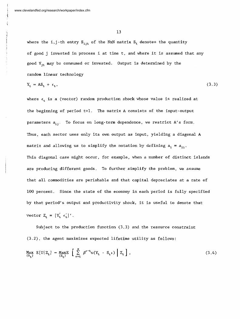
where the i , j - t h entry Sijt of the NxN matrix St denotes the quantity

of good j invested i n process i a t time t , and where it i s assumed tha t any

good Yjt may be consumed or invested. Output i s determined by the

random l inear technology

Yt =ASt + E,, (3.3)

where et i s a (vector) random production shock whose value i s realized a t

the beginning of period t + l . The matrix A consists of the input-output

parameters ai j . To focus on long-term dependence, we r e s t r i c t A's form.

Thus, each sector uses only i t s own output as input, yielding a diagonal A

matrix and allowing us to simplify the notation by defining ai = aii.

This diagonal case might occur, for example, when a number of d i s t inc t islands

are producing dif ferent goods. To further simplify the problem, we assume

tha t a l l commodities are perishable and that capi ta l depreciates a t a ra te of

100 percent. Since the s t a t e of the economy in each period i s fu l ly specified

by tha t period's output and productivity shock, it i s useful to denote that

vector Z, = [Y; E L ] ' .

Subject to the production function (3.3) and the resource constraint

(3 .2 ) , the agent maximizes expected lifetime u t i l i t y as follows:

Max E[UI Zt] = MaxE [ f /37-tu(~t - St') I Zt ] , {St} {St) 7=t


14

where we have substituted for consumption in (3.4) using the budget equation

(3.2). This maps naturally into a dynamic programming formulation, with a

value function V(Zt) and optimality equation

With quadratic utility and linear production, it is straightforward to

discover and verify the form of V(Zt):

V(Y,E) - q'Y + Y'PY + R + E[E'TE], (3.6)

where q and R &note Nxl vectors and P and T are NxN matrices, with entries

being fixed constants given by the matrix Riccati equation resulting from the

value function's recursive definition.' Given the value function, the

first-order conditions of the optimality equation (3.5) yield the chosen

quantities of consumption and investment/savings and, for the example

presented here, have the following closed-form solutions:

and

where


The simple form of the optimal consumption and investment decision rules comes

from the quadratic preferences and the linear production function. Two

qualitative features bear emphasizing. First, higher output today will

increase both current consumption and current investment, thus increasing

future output. Even with 100 percent depreciation, no durable commodities,

and i.i.d. production shocks, the time-to-build feature of investment induces

serial correlation. Second, the optimal choices do not depend on the

uncertainty that is present. This certainty equivalence feature is clearly an

artifact of the linear-quadratic combination.

The time series of output can now be calculated from the production

function (3.1) and the decision rule (3.7). Quantity dynamics then come from

the difference equation

where Ki is some fixed constant. The key qualitative property of quantity

dynamics summarized by (3.11) is that output Yi, follows an AR(1) process.


16

Higher output today implies higher output in the future. That effect dies off

at a rate that depends on the parameter ai, which in turn depends on the

underlying preferences and technology.

The simple output dynamics for a single industry or island neither mimics

business cycles nor exhibits long-run dependence. However, aggregate output,

the sum across all sectors, does show such dependence, which we demonstrate

here by applying the aggregation results of Granger (1980, 1988).

It is well known that the sum of two series Xt and Y,, each AR(1) with

independent error, is an ARMA(2,l) process. Simple induction then implies

that the sum of N independent AR(1) processes with distinct parameters has an

ARMA(N,N-1) representation. With more than six million registered businesses

in America (Council of Economic Advisors, 1988), the dynamics can be

incredibly rich - - and the number of parameters unmanageably huge. The common

response to this problem is to pretend that many different firms (islands)

have the same AR(1) representation for output, which reduces the dimensions of

the aggregate ARMA process. This "canceling of roots" requires identical

autoregressive parameters. An alternative approach reduces the scope of the

problem by showing that the ARMA process approximates a fractionally

integrated process and thus summarizes the many ARMA parameters in a

parsimonious manner. Though we consider only the case of independent sectors,

dependence is easily handled.

Consider the case of N sectors, with the productivity shock for each

serially uncorrelated and independent across islands. Furthermore, let the

sectors differ according to the productivity coefficient ai. This implies


17

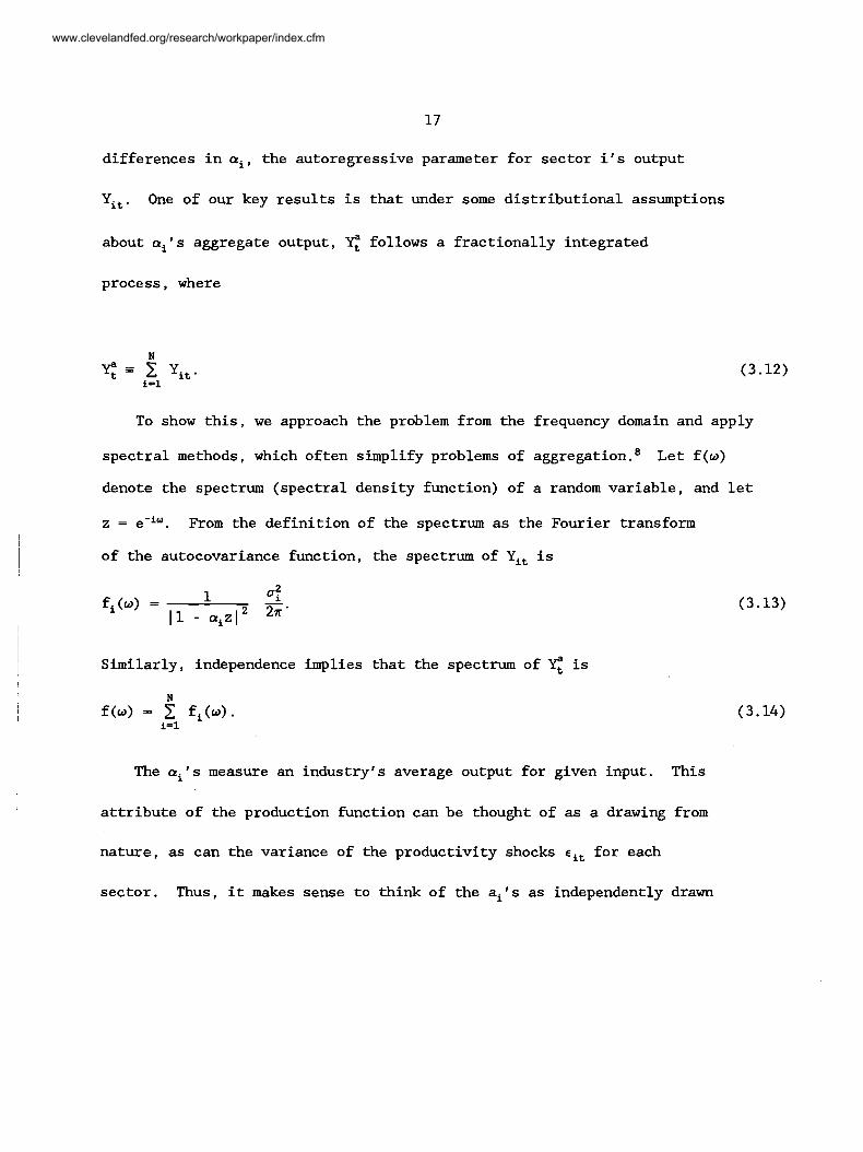
differences in ai, the autoregressive parameter for sector i's output

Yi,. One of our key results is that under some distributional assumptions

about ails aggregate output, 3 follows a fractionally integrated

process, where

To show this, we approach the problem from the frequency domain and apply

spectral methods, which often simplify problems of aggregation. Let f (w)

denote the spectrum (spectral density function) of a random variable, and let

z = e-iw. From the definition of the spectrum as the Fourier transform

of the autocovariance function, the spectrum of Yit is

Similarly, independence implies that the spectrum of 3 is

The ails measure an industry's average output for given input. This

attribute of the production function can be thought of as a drawing from

nature, as can the variance of the productivity shocks tit for each

sector. Thus, it makes sense to think of the airs as independently drawn


18

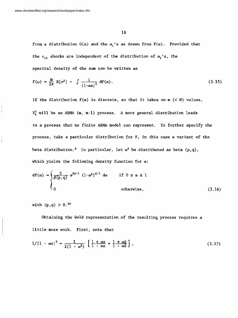
from a distribution G(a) and the ai's as drawn from F(a). Provided that

the E , , shocks are independent of the distribution of a,'~, the

spectral density of the sum can be written as

If the distribution F(a) is discrete, so that it takes on m (< N) values,

Y: will be an ARMA (m, m-1) process. A more general distribution leads

to a process that no finite ARMA model can represent. To further specify the

process, take a particular distribution for F, in this case a variant of the

beta distrib~tion.~ In particular, let a2 be distributed as beta (p,q),

which yields the following density function for a:

( 0 otherwise,

with (p, q) > 0. lo

Obtaining the Wold representation of the resulting process requires a

little more work. First, note that


19

where 2 denotes the complex conjugate of z, and the terms in brackets can

be further expanded by long division. Substituting this expansion and the

beta distribution (3.16) into the expression for the spectrwn and simplifying

(using the relation z + 2 = 2 cos(w)) yields

Then, the coefficient of cos(h) is

Since the spectral density is the Fourier transform of the autocovariance

function, (3.19) is the k-th autocovariance of 3. Furthermore,

because the integral defines a beta function, (3.19) simplifies to /3(p+k/2,

q - 1)/ /3(p,q). Dividing by the variance gives the autocorrelation

coefficients, which reduce to

Using the result from S tirling ' s approximation r(a+k)/r(b+k) = ka-b,

(3.20) is proportional (for large lags) to kl-q. Thus, aggregate output

Y: follows a fractionally integrated process of the order d = 1 - Q 2 '


20

Furthermore, as an approximation for long lags, this does not necessarily rule

out interesting correlations at higher, e.g., business cycle, frequencies.

Similarly, comovements can arise as the fractionally integrated income process

induces fractional integration in other observed time series. This phenomenon

has been generated by a maximizing model based on tastes and

technologies. l1

In principle, all of the model's parameters may be estimated, from the

distribution of production functions to the variance of output shocks.

Although to our knowledge no one has explicitly estimated the distribution of

production function parameters, many people have estimated production

functions across industries.12 (One of the better recent studies

disaggregates to 45 industries.13) For our purposes, the quantity

closest to a, is the value-weighted intermediate-product factor share.

Using a translog production function, this gives the factor share of inputs

coming from industries, excluding labor and capital. These inputs range from

a low of 0.07 for radio and television advertising to a high of 0.81 for

petroleum and coal products. Thus, even a small amount of disaggregation

reveals a large dispersion, suggesting the plausibility and significance of

the simple model presented in this section.

Although the original motivation for our real business cycle model was to

illustrate how long-range dependence could arise naturally in an economic

system, our results have broader implications for general macroeconomic

modeling. They show that moving to a multiple-sector real business cycle

model introduces not unmanageable complexity, but qualitatively new behavior


21

that in some cases can be quite manageable. Our findings also show that

calibrations aimed at matching only a few first and second moments can

similarly hide major differences between models and the data, missing long-run

dependence properties. While widening the theoretical horizons of the

paradigm, fractional techniques also widen the potential testing of such

theories.

3.2. Fiscal Policy and Welfare Implications

Taking a policy perspective raises two natural questions about the

fractional properties of national income. First, will fiscal or monetary

policy change the degree of long-term dependence? Friedman and Schwartz

(1982), for example, point out that long-run income cycles correlate with

long-run monetary cycles. Second, does long-term dependence have welfare

implications? Do agents care that they live in such a world?

In the basic Ramsey-Solow growth model, as in its stochastic extensions,

taxes affect output and capital levels but not growth rates; thus, tax policy

does not affect fractional properties. l4 However, two alternative

approaches suggest richer possibilities. First, recall that fractional noise

arises through the aggregation of many autoregressive processes. Fiscal

policy may not change the coefficients of each process, but a tax policy can

alter the distribution of total output across individuals, effectively

changing the fractional properties of the aggregate. Second, endogenous

growth models often allow tax policy to affect growth rates by reducing

investment in research, thus depressing future growth. l5 Hence, the


22

autoregressive parameters of an individual firm's output could change with

policy, in turn affecting aggregate income.

Unfortunately, implementing either approach with even a modicum of realism

would be quite complicated. In the dynamic stochastic growth model, taxation

drives a wedge between private and social returns, resulting in a suboptimal

equilibrium. This eliminates methods that exploit the pareto-optimality of

competitive equilibrium, such as dynamic programming. Characterizing

solutions requires simulation methods, because no closed forms have been

found.16 Thus, it seems clear that fiscal policy can affect fractional

properties. Explicitly calculating the impact would take this paper too far

afield and is best left for future research.

Those who forecast output or sales will care about the fractional nature

of output, but fractional processes can have normative implications as well.

Following Lucas (1987), this section estimates the welfare costs of economic

instability under different regimes. We can decide if people care whether

their world is fractional. For concreteness, let the typical household

consume C,, evaluating this via a utility function:

Also assume that

m


2 3

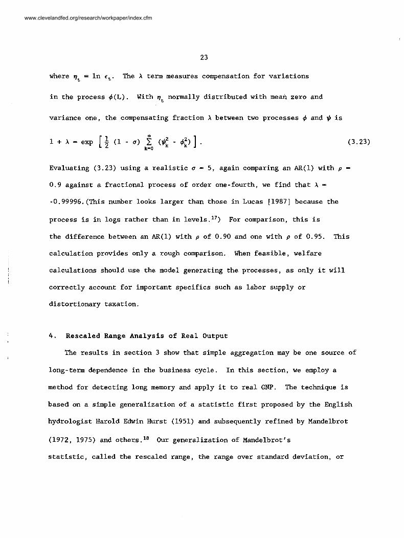
where 9, = In r , . The X term measures compensation for variations

in the process 4(L). With 9, normally distributed with mean zero and

variance one, the compensating fraction X between two processes 4 and 1/, is

m 1 + X = exp [ $ (1 - 0) 1 (1/,: - 43 ] - (3.23)

k=O

Evaluating (3.23) using a realistic a = 5, again comparing an AR(1) with p =

0.9 against a fractional process of order one-fourth, we find that X =

-0.99996.(This number looks larger than those in Lucas [1987] because the

process is in logs rather than in levels.17) For comparison, this is

the difference between an AR(1) with p of 0.90 and one with p of 0.95. This

calculation provides only a rough comparison. When feasible, welfare

calculations should use the model generating the processes, as only it will

correctly account for important specifics such as labor supply or

distortionary taxation.

4. Rescaled Range Analysis of Real Output

The results in section 3 show that simple aggregation may be one source of

long-term dependence in the business cycle. In this section, we employ a

method for detecting long memory and apply it to real GNP. The technique is

based on a simple generalization of a statistic first proposed by the English

hydrologist Harold Edwin Hurst (1951) and subsequently refined by Mandelbrot

(1972, 1975) and others.18 Our generalization of Mandelbrot's

statistic, called the rescaled range, the range over standard deviation, or


24

the R/S statistic, enables us to distinguish between short- and long-run

dependence, in a sense that will be made precise below. We define our notions

of short and long memory and present the test statistic in section 4.1.

Section 4.2 gives the empirical results for real GNP. We find long-term

dependence in log-linearly detrended output, but considerably less dependence

in the growth rates. To interpret these findings, we perform several Monte

Carlo experiments under two null and two alternative hypotheses. Results are

reported in section 4.3.

4.1. The R/S Statistic

To develop a method of detecting long memory, we must be precise about the

distinction between long- term and short- term statistical dependence. One of

the most widely used concepts of short-term dependence is the notion of

"strong-mixing" (based on Rosenblatt [1956]), a measure of the decline in

statistical dependence of two events separated by successively longer time

spans. Heuristically, a time series is strong-mixing if the maximal

dependence between any two events becomes trivial as more time elapses between

them. By controlling the rate at which the dependence between future events

and those of the distant past declines, it is possible to extend the usual

laws of large numbers and central-limit theorems to dependent sequences of

random variables. Such mixing conditions have been used extensively by White

(1980), White and Domowitz (1984), and Phillips (1987), for example, to relax

the assumptions that ensure consistency and asymptotic normality of various

econometric estimators. We adopt this notion of short-term dependence as part


2 5

of our null hypothesis. As Phillips (1987) observes, these conditions are

satisfied by a great many stochastic processes, including all Gaussian

finite-order stationary ARMA models. Moreover, the inclusion of a moment

condition allows for heterogeneously distributed sequences (such as those

exhibiting heteroscedasticity) , an especially important extension in view of

the nonstationarities of real GNP.

In contrast to the "short memory" of weakly dependent (i.e.,

strong-mixing) processes, natural phenomena often display long-term memory in

the form of nonperiodic cycles. This has led several authors, most notably

Mandelbrot, to develop stochastic models that exhibit dependence even over

very long time spans. The fractionally integrated time-series models of

Mandelbrot and Van Ness (1968), Granger and Joyeux (1980), and Hosking (1981)

are examples of these. Operationally, such models possess autocorrelation

functions that decay at much slower rates than those of weakly dependent

processes, violating the conditions of strong-mixing. To detect long-term

dependence (also called strong dependence), Mandelbrot suggests using the R/S

statistic, which is the range of partial sums of deviations of a time series

from its mean, rescaled by its standard deviation. In several seminal papers,

Mandelbrot demonstrates the superiority of the R/S statistic over more

conventional methods of determining long- run dependence, such as

autocorrelation analysis and spectral analysis. l9

In testing for long memory in output, we employ a modification of the R/S

statistic that is robust to weak dependence. In Lo (1991), a formal sampling

theory for the statistic is obtained by deriving its limiting distribution


analytically using a functional central-limit theorem. 20 We use this

statistic and its asymptotic distribution for inference below. Let Xt

denote the first difference of log-GNP; we assume that

where p is an arbitrary but fixed parameter. Whether or not X, exhibits

long-term memory depends on the properties of E,. For the null hypothesis

H, the sequence of disturbances E, satisfies the following conditions:

(Al) E[et] = 0 for all t.

(A2) sup E[ JE,~'] < a for some p > 2. t

exists, and u2 > 0

(A4) ( E ~ ) is strong-mixing, with mixing coefficients % that

satisfy21

Condition (Al) is standard. Conditions (A2) through (A4) are restrictions

on the maximal degree of dependence and heterogeneity allowable while still

permitting some form of the law of large numbers and the (functional)

central-limit theorem to obtain. Note that we have not assumed stationarity.

Although condition (A2) rules out infinite-variance marginal distributions of

E ~ , such as those in the stable family with characteristic exponent less

than two, the disturbances may still exhibit leptokurtosis via time-varying


2 7

conditional moments (e.g., conditional heteroscedasticity). Moreover, since

there is a trade-off between conditions (A2) and (A4), the uniform bound on

the moments may be relaxed if the mixing coefficients decline faster than (A4)

requires .22 For example, if we require 6 , to have finite absolute

moments of all orders (corresponding to /3 + co), then % must decline

faster than l/k. However, if we restrict 6 , to have finite moments only up

to order four, then % must decline faster than l/k2. These conditions

are discussed at greater length in Phillips (1987), to which we refer

interested readers.

Conditions (Al) through (A4) are satisfied by many of the recently

proposed stochastic models of persistence, such as the stationary AR(1) with a

near-unit root. Although the distinction between dependence in the short

versus the long run may appear to be a matter of degree, strongly dependent

processes behave so differently from weakly dependent ones that our dichotomy

seems quite natural. For example, the spectral densities of strongly

dependent processes are either unbounded or zero at frequency zero. Their

partial sums do not converge in distribution at the same rate as weakly

dependent series, and graphically, their behavior is marked by cyclic patterns

of all kinds, some that are virtually indistinguishable from trends.23

To construct the modified R/S statistic, consider a sample XI, 3,

1 . . . , X,, and let En denote the sample mean lj X,. Then, the modified R/S statistic, which we shall call a, is given by


k k a=- [x, - gn) - Min 1 [xj - a,)], - j=l where

2 and 6, and 7 are the usual sample variance and autocovariance estimators j

of X. Q,, is the range of partial sums of deviations of Xj from its mean,

k, normalized by an estimator of the partial sum's standard deviation divided by n. The estimator 3,(q) involves not only sums of squared

deviations of Xj, but also its weighted autocovariances up to lag q; the

weights wj(q) are those suggested by Newey and West (1987), and they always

2 yield a positive estimator 6,(q) .24 Theorem 4 . 2 in Phillips

(1987) demonstrates the consistency of 3,(q) under the following

conditions :

(A2') supt ~[lr,~~'] < for some B > 2 .

(A5) As n increases without bound, q also rises without bound, such that

- o(n1/4 .


2 9

The choice of the truncation lag q is a delicate matter. Although q must

increase with the sample size (although at a slower rate), Monte Carlo

evidence suggests that when q becomes large relative to the number of

observations, asymptotic approximations may fail dramatically. If the

chosen q is too small, however, the effects of higher-order autocorrelations

may not be captured. Clearly, the choice of q is an empirical issue that muust

take into account the data at hand.

Under conditions (Al), (A2'), (A3) . . . A(5), Lo (1991) shows that the

statistic V,, = has a well-defined asymptotic distribution given by

the random variable V, whose distribution function Fv (v) isz6

Using F,, critical values may be readily calculated for tests of any

significance level. The most commonly used values are reported in tables la

and lb. Table la reports the fractiles of the distribution, while table lb

reports the symmetric confidence intervals about the mean. The moments of V

are also easily computed using the density function fv; it is

2 7r2 straightforward to show that E[V] = $ and E[V ] = -. Thus, 6


30

the mean and standard deviation of V are approximately 1.25 and 0.27,

respectively. The distribution and density functions are plotted in figure 4.

Note that the distribution is positively skewed and that most of its mass

falls between three-fourths and two.

If the obsemations are independently and identically distributed with

variance a:, our normalization by 3,(q) is asymptotically equivalent to

1 normalizing by the usual standard deviation estimator sn = [ii lj(xj - En)2]1'2.

The resulting statistic, which we call on, is precisely the one proposed

by Hurst (1951) and Mandelbrot (1972):

k k O n 2 [ Max 1 X j - E n - Min 1 (xj - En}] . 'n j=l 1 9 5 1 1 j=l

Under the more restrictive null hypothesis of i.i.d. observations, the

statistic vn = Gn/fi can be shown to converge to V as well. However, in

the presence of short-range dependence, vn does not converge to V, whereas Vn still does. Of course, if the particular form of short-range

dependence is known, it can be accounted for in deriving the limiting

distribution of vn. For example, if Xt is a stationary AR(1) with

autoregressive parameter p, Lo (1991) shows that vn converges to (V,

where ( = *j(l+p)/(l-p). But since we would like our limiting


31

distribution to be robust to general forms of short-range dependence, we

use the modified R/S statistic Vn below.

4.2. Empirical Results for Real Output

We apply our test to two time series of real output: quarterly postwar

real GNP from 1947:IQ to 1987:IVQ, and the annual Friedman and Schwartz (1982)

series from 1869 to 1972. These results are reported in table 2. Entries in

the first numerical row are estimates of the classical R/S statistic f,,

which is not robust to short-term dependence. The next eight rows are

estimates of the modified R/S statistic Vn(q) for values of q from one to

eight. Recall that q is the truncation lag of the spectral density estimator

at frequency zero. Reported in parentheses below the entries for Vn(q) are

estimates of the percentage bias of the statistic qn, computed as

100 [fn/vn(q> - 11.

The first column of numerical entries in table 2 indicates that the null

hypothesis of short-term dependence for the first difference of log-GNP cannot

be rejected for any value of q. The classical R/S statistic also supports the

null hypothesis, as do the results for the Friedman and Schwartz series. On

the other hand, when we log-linearly detrend real GNP, the results are

considerably different. The third column of numerical entries in table 2

shows that short-term dependence may be rejected for log-linearly detrended

quarterly output with values of q from one to four. That the rejections are

weaker for larger q is not surprising, since additional noise arises from

estimating higher-order autocorrelations. When values of q beyond four are


3 2

used, we no longer reject the null hypothesis at the 5 percent level of

significance. Finally, using the Friedman and Schwartz time series, we only

reject with the classical R/S statistic and with V,(l).

The values reported in table 2 are qualitatively consistent with the

results of other empirical studies of fractional processes in GNP, such as

Diebold and Rudebusch (1989) and Sowell (1989). For first differences, the

R/S statistic falls below the mean, suggesting a negative fractional exponent,

or in level terms, an exponent between zero and one. Furthermore, though the

earlier papers produce point estimates, the imprecision of these estimates

means that they do not reject the hypothesis of short-term dependence. For

example, the standard-deviation error bounds for Diebold and Rudebusch's

two point estimates, d = 0.9 and d = 0.52, are (0.42, 1.38) and (0.06, 1.10),

respectively.

Taken together, our results confirm the unit-root findings of Campbell and

Mankiw (1987), Nelson and Plosser (1982), Perron and Phillips (1987), and

Stock and Watson (1986). That there are more significant autocorrelations in

log-linearly detrended GNP is precisely the spurious periodicity suggested by

Nelson and Kang (1981). Moreover, the trend plus stationary noise model of

GNP is not contained in our null hypothesis; hence, our failure to reject the

null hypothesis is also consistent with the unit-root model .27 To see

this, observe that if log-GNP y were trend stationary, i.e., if t


33

where r,~, is stationary white noise, then its first difference X, would

simply be X, = /3 + r , , where r , = 'It - But this innovations

process violates our assumption (A3) and is therefore not contained in our

null hypothesis.

Sowell (1989) has used estimates of d to argue that the trend-stationary

model is correct. Following the lead of Nelson and Plosser (1982), he

investigates whether the d parameter for the first-differenced series is close

to zero, as the unit-root specification suggests, or close to minus one, as

the trend-stationary specification suggests. His estimate of d is in the

general range of -0.9 to -0.5, providing some evidence that the

trend-stationary interpretation is correct. Even in this case, however, the

standard errors tend to be large, on the order of 0.36. Although our

procedure yields no point estimate of d, it does seem to rule out the

trend-stationary case.

To conclude that the data support the null hypothesis because our

statistic fails to reject it is premature, of course, since the size and power

of our test in finite samples is yet to be determined.

4.3. Size and Power of the Test

To evaluate the size and power of our test in finite samples, we perform

several illustrative Monte Carlo experiments for a sample of 163 observations,

which corresponds to the number of quarterly observations of real GNP growth

from 1947: IQ to 1987: I V Q . ~ ~ We simulate two null hypotheses:


independently and identically distributed increments, and increments that

follow an ARMA(2,2) process. Under the i.d.d. null hypothesis, we fix the

mean and standard deviation of our random deviates to match the sample mean

and standard deviation of our quarterly data set: 7.9775 x and

1.0937 x respectively. To choose parameter values for the

ARMA(2,2) simulation, we estimate the model

using nonlinear least squares. The parameter estimates are as follows

(standard errors are in parentheses):

Table 3 reports the results of both null simulations.

It is apparent from the i.i.d. null panel of table 3 that the 5 percent

test based on the classical R/S statistic rejects too frequently. The 5

percent test using the modified R/S statistic with q = 3 rejects 4 . 6 percent

of the time, closer to the nominal size. As the number of lags increases to

eight, the test becomes more conservative. Under the ARMA(2,2) null

hypothesis, it is apparent that modifying the R/S statistic by the spectral


2 density estimator &,(q) is critical. The size of a 5 percent test based on the

classical R/S statistic is 34 percent, whereas the corresponding size using

the modified R/S statistic with q = 5 is 4.8 percent. As before, the test

becomes more conservative when q is increased.

Table 3 also reports the size of tests using the modified R/S statistic

when the lag length q is optimally chosen using Andrews' (1987) procedure.

This data-dependent procedure entails computing the first-order

autocorrelation coefficient j(1) and then setting the lag length as the

integer value of fin, wherez9

Under the i.i.d. null hypothesis, Andrews' formula yields a 5 percent test

with empirical size 6.9 percent; under the ARMA(2,2) alternative, the

corresponding figure is 4.1 percent. Although significantly different from

the nominal value, the empirical size of tests based on Andrews' formula may

not be economically important. In addition to its optimality properties, the

procedure has the advantage of eliminating a dimension of arbitrariness from

the test. Table 4 reports power simulations under two fractionally differenced

d alternatives: (1 - L) et = qt, where d = (1/3, -1/3). Hosking (1981)

has shown that the autocovariance function yc(k) equals


Realizations of fractionally differenced time series of length 163 are

simulated by pre-multiplying vectors of independent standard normal random

variates by the Cholesky factorization of the 163 x 163 covariance matrix,

whose entries are given by (3.11). To calibrate the simulations, a:

is chosen to yield unit variance E,. We then multiply the e, series by

the sample standard deviation of real GNP growth from 1947:IQ to 1987:IVQ and

add the sample mean of real GNP growth over the same period. The resulting

time series is used to compute the power of the R/S statistic (see table 4).

For small values of q, tests based on the modified R/S statistic have

reasonable power against both of the fractionally differenced alternatives.

For example, using one lag, the 5 percent test has 58.7 percent power against

the d = 1/3 alternative and 81.1 percent power against the d = -1/3

alternative. As the lag is increased, the test's power declines.

Note that tests based on the classical R/S statistic are significantly

more powerful than those using the modified R/S statistic. This, however, is

of little value when distinguishing between long-term and short-term

dependence, since the test using the classical statistic also has power

against some stationary finite-order ARMA processes. Finally, note that tests

using Andrews' truncation lag formula have reasonable power against the d =

-1/3 alternative, but are considerably weaker against the more relevant d =

1/3 alternative.


37

The simulation evidence in tables 3 and 4 suggests that our empirical

results do indeed support the short-term dependence of GNP with a unit root.

Our failure to reject the null hypothesis does not seem to be explicable by a

lack of power against long-memory alternatives. Of course, our simulations

are illustrative and by no means exhaustive; additional Monte Carlo

experiments will be required before a full assessment of the test's size and

power is complete. Nevertheless, our modest simulations indicate that there

is little empirical evidence of long-term memory in GNP growth rates. Perhaps

a direct estimation of long-memory models would yield stronger results, an

issue that has recently been investigated by several authors.30

5 . Conclus ion

This paper has suggested a new approach for investigating the stochastic

structure of aggregate output. Traditional dissatisfaction with conventional

methods - - from observations about the typical spectral shape of economic time

series to the discovery of cycles at all periods - - calls for such a

reformation. Indeed, recent controversy about deterministic versus stochastic

trends and the persistence of shocks underscores the difficulties even modem

methods have in identifying the long-run properties of the data.

Fractionally integrated random processes provide one explicit approach to

the problem of long-term dependence; naming and characterizing this aspect is

the first step in studying the problem scientifically. Controlling for

long-term dependence improves our ability to isolate business cycles from

trends and to assess the propriety of that decomposition. To the extent that


3 8

long-term dependence explains output, it deserves study in its own right.

Furthermore, Singleton (1988) has pointed out that dynamic macroeconomic

models often inextricably link predictions about business cycles, trends, and

seasonal effects. So, too, is long-term dependence linked: A fractionally

integrated process arises quite naturally in a dynamic linear model via

aggregation. Our model not only predicts the existence of fractional noise,

but suggests the character of its parameters. This class of models leads to

testable restrictions on the nature of long-term dependence in aggregate data,

and also holds the promise of enhancing policy evaluation.

Advocating a new class of stochastic processes would be a fruitless task

if its members were intractable. But in fact, manipulating such processes

causes few problems. We construct an optimizing linear dynamic model that

exhibits fractionally integrated noise, and provide an explicit test for such

long-term dependence. Modifying a statistic developed by Hurst and Mandelbrot

gives us a statistic robust to short-term dependence. This modified R/S

statistic possesses a well-defined limiting distribution, which we have

tabulated. Illustrative computer simulations indicate that this test has

power against at least two specific alternative hypotheses of long-term

memory.

Two main conclusions arise from our empirical work and from Monte Carlo

experiments. First, the evidence does not support long-term dependence in

GNP. Rejections of the short- term-dependence null hypothesis occur only with

detrended data and are consistent with the well-known problem of spurious

periodicities induced by log-linear detrending. Second, since a


39

trend-stationary model is not contained in our null hypothesis, our failure to

reject may also be viewed as supporting the first-difference stationary model

of GNP, with the additional result that the stationary process is at best

weakly dependent. This supports and extends Adelman's conclusion that, at

least within the confines of the available data, there is little evidence of

long-term dependence in the business cycle.


Footnotes

1. The idea of fractional differentiation is an old one (dating back to an oblique reference by Leibniz in 1695), but the subject lay dormant until the nineteenth century, when Abel, Liouville, and Riemann developed it more fully. Extensive applications have only arisen in this century; see, for example, Oldham and Spanier (1974). Kolmogorov (1940) was apparently the first to notice its applicability in probability and statistics.

2. When d is an integer, (2.3) reduces to the better-known formula for the

binomial coefficient, d! k! (d-k) ! ' We follow the convention that

(8) = 1 and (8) = 0.

3. See Hosking (1981) for further details.

4. See Cochrane (1988) andQuah (1987) for opposing views.

5. There has been some confusion about this point in the literature. Geweke and Porter-Hudak (1983) argue that C(l) > 0. They correctly point out that Granger and Joyeux (1980) erred, but then incorrectly claim that (1) = 1 ) If our equation (2.7) is correct, then it is apparent that C(l) = 0 (which agrees with Granger [I9801 and Hosking [1981]). Therefore, the focus of the conflict lies in the approximation of the ratio r(k+d)/r(k+l) for large k. We have used Stirling's approximation. However, a more elegant derivation follows from the functional analytic definition of the gamma function as the solution to the following recursive relation (see, for example, Iyanaga and Kawada [1980, section 179.A]) :

r(x+i) = x~(x)

and the conditions

r(x+n) - 1. r(1) = 1 lim - - n - . ~ nxI'(n)

6. See Chatfield (1984, chapters 6 and 9).

7. See Sargent (1987, chapter 1) for an excellent exposition.

8. See Theil (1954).

9. Granger (1980) conjectures that this particular distribution is not essential.

10. For a discussion of the variety of shapes the beta distribution can take as p and q vary, see Johnson and Kotz (1970).


Two additional points are worth emphasizing. First, the beta

distribution need not be over (0,l) to obtain these results, only over

( 1 ) Second, it is indeed possible to vary the aifs so that ai

has a beta distribution.

Leontief, in his classic (1976) study, reports own-industry output coefficients for 10 sectors, investigating how much an extra unit of food will increase food production. Results vary from 0.06 (fuel) to 1.24 (other industries).

See Jorgenson, Gollop, and Fraumeni (1987).

See Atkinson and Stiglitz (1980).

For example, see Romer (1986) and King, Plosser, and Rebelo (1987).

See King, Plosser, and Rebelo (1987), Baxter (1988), and Greenwood and Huffman (1991).

We calculate this using (2.7) and the Hardy-Littlewood approximation for the resulting Rieman Zeta Function, following Titchmarsh (1951, section 4.11).

See Mandelbrot and Taqqu (1979) and Mandelbrot and Wallis (1968, 1969a-c) .

See Mandelbrot (1972, 1975), Mandelbrot and Taqqu (1979), and Mandelbrot and Wallis (1968, 1969a-c).

This statistic is asymptotically equivalent to Mandelbrot's under independently and identically distributed observations. However, Lo (1991) shows that the original R/S statistic may be significantly biased toward rejection when the time series is short-term dependent. Although aware of this bias, Mandelbrot (1972, 1975) did not correct for it, since his focus was on the relation of the R/S statistic's logarithm to the logarithm of the sample size, which involves no statistical inference; such a relation clearly is unaffected by short-term dependence.

Let ( E ~ ( w ) ) be a stochastic process on the probability space (fl,

F, P) and define

a(A,B) = sup IP(AnB) - P(A)P(B)I AcF,BcF

(A-l,Wl The quantity a(A,B) is a measure of the dependence between the two

a fields A and B in F. Denote by B: the Bore1 a field generated


t by [E,(w), . . . , E~(w)], i.e., B, = u[E,(w), . . . , E~(w)] c F. Define the coefficients cr, as

cr, = sup a (B'-~, B " ) . j +k

j

Then, (E,(w)) is said to be strong-mixing if lim cr, = 0. 0.00

For further details, see Rosenblatt (1956), White (1984), and the papers in Eberlein and Taqqu (1986).

See Herndorf (1985). Note that one of Mandelbrot's (1972) arguments in favor of R/S analysis is that finite second moments are not required. This is indeed the case if we are interested only in the almost sure convergence of the statistic. However, since we wish to derive its limiting distribution for purposes of inference, a stronger moment condition is needed.

See Mandelbrot (1972) for further details.

ui(q) is also an estimator of the spectral density function of

Xt at frequency zero, using a Bartlett window.

See, for example, Lo and MacKinlay (1988).

V may be shown to be the range of a Brownian bridge on the unit interval. See Lo (1991) for further details.

Of course, this may be the result of low power against stationary but near-integrated processes, an issue that must be addressed by Monte Carlo experiments.

All simulations were performed in double precision on a VAX 8700 using the IMSL 10.0 random number generator DRNNOA. Each experiment consisted of 10,000 replications.

In addition, Andrews' procedure requires weighting the autocovariances by

j (j = 1, . . . , [%I ) , in contrast to Newey and West's (1987)

1 - 1 (j = 1, . . . , q), where q is an integer but (4) need not be. q+l

See, for example, Diebold and Rudebusch (1989), Sowell (1987), and Yajima (1985, 1988).


4 3

References

Adelman, Irma (1965): "Long Cycles: Fact or Artifact?" American

Economic Review 55, 444-463.

Andrews, Donald (1987): "Heteroskedasticity and Autocorrelation Consistent Covariance Matrix Estimation," Working Paper, Cowles Foundation, Yale University.

Atkinson, Anthony B., and Joseph E. Stiglitz (1980): Lectures on Public

Economics. New York: McGraw-Hill.

Baxter, Marianne (1988): "Approximating Suboptimal Dynamic Equilibria: A Euler Equation Approach," Working Paper, University of Rochester.

Beveridge, Stephen, and Charles R. Nelson (1981): "A New Approach to Decomposition of Economic Time Series into Permanent and Transitory Components, with Particular Attention to Measurement of the 'Business Cycle'," Journal of Monetary Economics 4, 151-174.

Campbell, John Y., and N. Gregory Mankiw (1987): "Are Output Fluctuations Transitory?" Quarterly Journal of Economics 102, 857-880.

Chatfield, Christopher (1984): The Analysis of Time Series: An

Introduction, 3d ed. New York: Chapman and Hall.

Cochrane, John (1988): "How Big Is the Random Walk in GNP?" Journal of Political Economy 96, 893-920.

Diebold, Francis X., and Glenn D. Rudebusch (1989): "Long Memory and Persistence in Aggregate Output, " Journal of Monetary Economics 24, 189 - 209.

Eberlein, Ernst, and Murad Taqqu (1986): Dependence in Probability and

Statistics, vol. 11, Progress in Probability and Statistics.

Birkhauser: Boston.


Fisher, Irving (1925): "Our Unstable Dollar and the So-Called Business Cycle," Journal of the American Statistical Association 20, 179- 202.

Friedman, Milton, and Anna J. Schwartz (1982): Monetary Trends in the

United States and the United Kingdom, NBER Monograph. Chicago: University of Chicago Press.

Geweke, John, and Susan Porter-Hudak (1983): "The Estimation and Application

of Long Memory Time Series Models," Journal of Time Series Analysis 4, 221-238.

Granger, Clive W. J. (1966): "The Typical Spectral Shape of an Economic Variable," Econometrica 37, 150-161.

(1980): "Long Memory Relations and the Aggregation of Dynamic Models," Journal of Econometrics 14, 227-238.

(1988): "Aggregation of Time Series Variables - - A Survey," Federal Reserve Bank of Minneapolis, Institute for Empirical Macroeconomics, Discussion Paper 1.

, and Roselyne Joyeux (1980): "An Introduction to Long-Memory Time Series Models and Fractional Differencing," Journal of Time Series Analysis 1, 14-29.

Greenwood, Jeremy, and Gregory W. Huffman (1991): "Tax Analysis in a Real-Business Cycle Model: On Measuring Harberger Triangles and Okun Gaps, " Journal of Monetary Economics 27, 167-190.

Hemdorf, Norbert (1985): "A Functional Central Limit Theorem for Strongly Mixing Sequences of Random Variables, " Zei tschrif t fuer Wahrscheinl ichkei tstheori e und Verwandte Gebiete 69, 541 -550.

Hosking, J.R.M. (1981): "Fractional Differencing," Biometrika 68, 165-176.

Hurst, Harold E. (1951): "Long Term Storage Capacity of Reservoirs," Transactions of the American Society of Civil Engineers 116, 770-799.


Iyanaga, Shokichi, and Yukiyosi Kawada, eds. (1977): Encyclopedic

Dictionary of Mathematics, Mathematical Society of Japan. Cambridge : Mass.: M.I.T. Press.

Johnson, Norman L., and Samuel Kotz (1970): Continuous Univariate Distributions, vol. 2. New York: John Wiley & Sons.

Jorgenson, Dale W., Frank M. Gollop, and Barbara M. Fraumeni (1987): Productivity and U. S . Economic Growth, Harvard Economic Studies, vol. 159. Cambridge, Mass.: Harvard University Press.

King, Robert G., Charles I. Plosser, and Sergio Rebelo (1987): "Production, Growth and Business Cycles," Working Paper, University of Rochester.

Kolmogorov, Andrei N. (1940): "Wienersche Spiralen und Einige Andere Interessante Kurven im Hilberteschen Raum," Comptes Rendus (Doklady) de lrAcadamie des Sciences de lrURSS 26, 115-118.

Kuznets, Simon (1965): Economic Growth and Structure. New York: Norton.

Kydland, Finn, and Edward C. Prescott (1982): "Time to Build and Aggregate Economic Fluctuations," Econometrica 50, 1345-1370.

Leontief, Wassily W. (1976): The Structure of the American Economy

1919-1939, 2d ed. White Plains, N.Y.: International Arts and Sciences Press, Inc.

Lo, Andrew. W. (1991): "Long-Term Memory in Stock Market Prices,"

Econometrica 59, 1279-1313.

, and A. Craig MacKinlay (1988): "The Size and Power of the Variance Ratio Test in Finite Samples: A Monte Carlo Investigation," Journal of Econometrics 40, 203-238.

Long, John B., Jr., and Charles I. Plosser (1983): "Real Business Cycles," Journal of Political Economy 91, 39-69.

Lucas, Robert E., Jr. (1987): Models of Business Cycles, Yrjo Jahnsson

Lectures. New York: Basil Blackwell.

Mandelbrot, Benoit (1972): "Statistical Methodology for Non-Periodic Cycles: From the Covariance to R/S Anslysis," Annals of Economic and

Social Measurement 1, 259-290.

(1975): "Limit Theorems on the Self-Normalized Range for Weakly and Strongly Dependent Processes," Zeitschrift fuer Wahrscheinlichkeitstheorie und Verwandte Gebiete 31, 271-285.


, and Murad Taqqu (1979): "Robust R/S Analysis of Long-Run Serial Correlation," Bul l e t i n o f t he Internat ional S t a t i s t i c a l I n s t i t u t e 48, Book 2, 59-104.

, and John Van Ness (1968), "Fractional Brownian Motion, Fractional Noises and Applications'," S.I.A.M. Review 10, 422-437.

, and James Wallis (1968): "Noah, Joseph and Operational Hydrology," Water Resources Research 4, 909-918.

, and James Wallis (1969a) : "Computer Experiments with Fractional Gaussian Noises," parts 1, 2, and 3, Water Resources Research 5, 228 - 267.

, and James Wallis (1969b): "Some Long Run Properties of Geophysical Records, " Water Resources Research 5, 321-340.

, and James Wallis (1969~): "Robustness of the Rescaled Range R/S in the Measurement of Noncyclic Long Run Statistical Dependence," Water Resources Research 5, 967-988.

Mitchell, Wesley Claire (1927): Business Cycles: The Problem and I t s S e t t i n g , NBER Studies in Business Cycles No. 1. New York: National Bureau of Economic Research.

Nelson, Charles R., and Heejoon Kang (1981): "Spurious Periodicity in Inappropriately Detrended Time Series," Econornetrica 49, 741-751.

, and Charles I. Plosser (1982): "Trends and Random Walks in Macroeconomic Time Series: Some Evidence and Implications," Journal o f Monetary Economics 10, 139-162.

Newey, Whitney K., and Kenneth D. West (1987): "A Simple, Positive Semi-Definite Heteroscedasticity and Autocorrelation Consistent Covariance Matrix," Econornetrica 55, 703-705.

Oldham, Keith B., and Jerome Spanier (1974): The Fractional Calculus. New York: Academic Press.

Perron, Pierre, and Peter C. B. Phillips (1987): "Does GNP Have a Unit Root?" Economic Le t t e r s 23, 139-145.

Phillips, Peter C. B. (1987): "Time Series Regression with a Unit Root," Econornetrica 55, 277- 301.

Quah, Danny (1987): "What Do We Learn from Unit Roots in Macroeconomic Time Series?" NBER Working Paper No. 2450.


Romer, Paul M. (1986): "Increasing Returns and Long-Run Growth," Journal of Political Economy 94, 1002-1037.

Rosenblatt, Murray (1956): "A Central Limit Theorem and a Strong Mixing Condition," Proceedings of the National Academy of Sciences 42, 43-47.

Sargent , Thomas J . (1987) : Dynamic Macroeconomic Theory. Cambridge, Mass.: Harvard University Press.

Singleton, Kenneth J. (1988): "Econometric Issues in the Analysis of Equilibrium Business Cycle Models, " Journal of Monetary Economics 21, 361-386.

Slutzky, Eugene (1937): "The Summation of Random Causes as the Source of Cyclic Processes," Econometrica 5, 105-146.

Sowell, Fallaw (1987a): "Fractional Unit Root Distributions," Discussion Paper No. 87-05, Institute of Statistics and Decision Sciences, Duke University.

(1989): "The Deterministic Trend in Real GNP," GSIA Working Paper No. 88-89-60, Carnegie-Mellon University.

Stock J., and M. Watson (1986): "Does GNP Have a Unit Root?" Economics Letters 22, 147-151.

Theil, Henri (1954): Linear Aggregation of'Economic Relations.

Amsterdam: North-Holland.

Titchmarsh, E. C. (1951) : The Theory of the Riemann Zeta-Function. Oxford, England: Clarendon Press.

White, Halbert (1980): "A Heteroscedasticity-Consistent Covariance Matrix Estimator and a Direct Test for Heteroscedasticity," Econometrica 48, 817-838.

(1984) : Asymptotic h he or^ for Econometricians. New York: John Wiley & Sons.

, and I. Domowitz (1984): "Nonlinear Regression with Dependent Observations," Econometrica 52, 143-162.

Yajima, Yoshihiro (1985): "On Estimation of Long-Memory Time Series Models," Australian Journal of Statistics, 303-320.

(1988): "On Estimation of a Regression Model with Long-Memory Stationary Errors," Annals of Statistics 16, 791-807.


- 475 0

pj f o r (I -L) - E t 7

m 0

z 0 - t 6 = 0

DL x 0 * g 0 t 3 Q

h]

0

0

0 0 30 60 90 120

LAG

Source : Authors

Figure 1

Autocorrelation functions of an AR(1) with coefficient 0.90 (dashed line) and

a fractionally differenced series X, = (1 - L ) - ~ c , with differencing parameter

d = 0.475 (solid line). Although both processes have a first-order

autocorrelation of 0.90, the fractionally differenced process decays much more

slowly.


Source: Authors

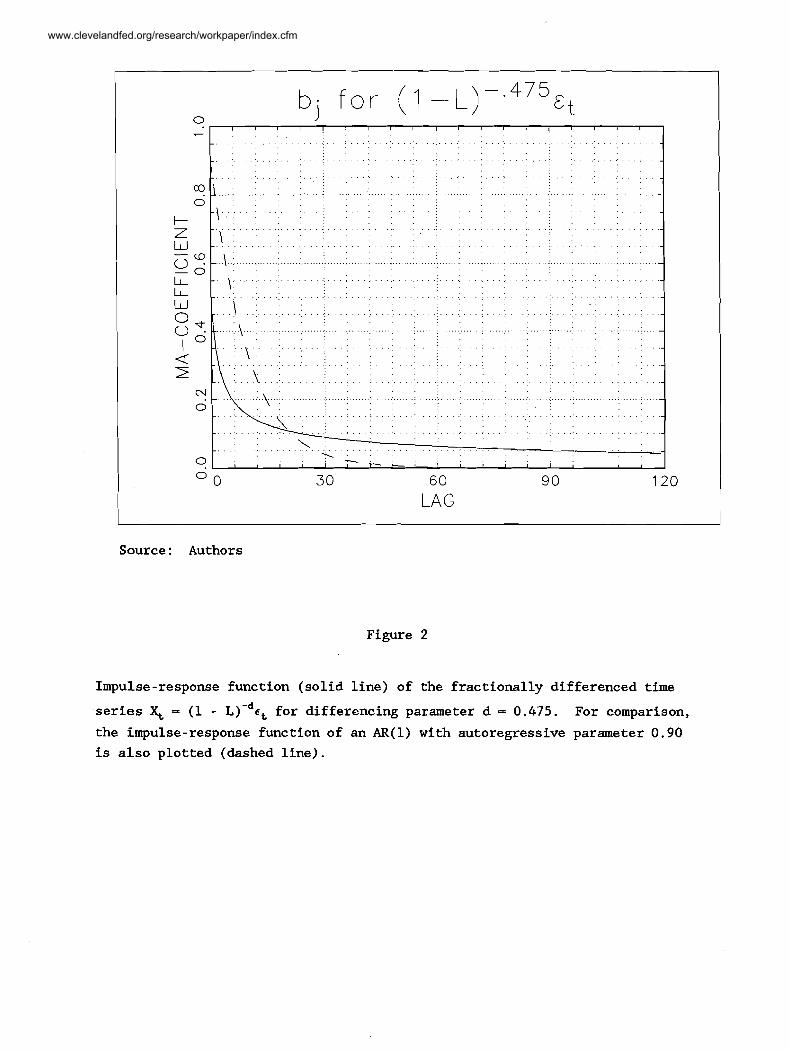
Figure 2

Impulse-response function (solid line) of the fractionally differenced time

series X, - (1 - L ) - ~ E ~ for differencing parameter d - 0.475. For comparison,

the impulse-response function of an AR(1) with autoregressive parameter 0.90

is also plotted (dashed line).


E q u i v a l e n t p o f A R ( I )

Source: Authors

. . . . . . . . . . . . . . . . - . \ . : . . . . . . . . . . . . . . r . . : . . . . . . . . . . . . . . . . I . . . - - . . . : . . . . . . : . . . . . . . . . . . .

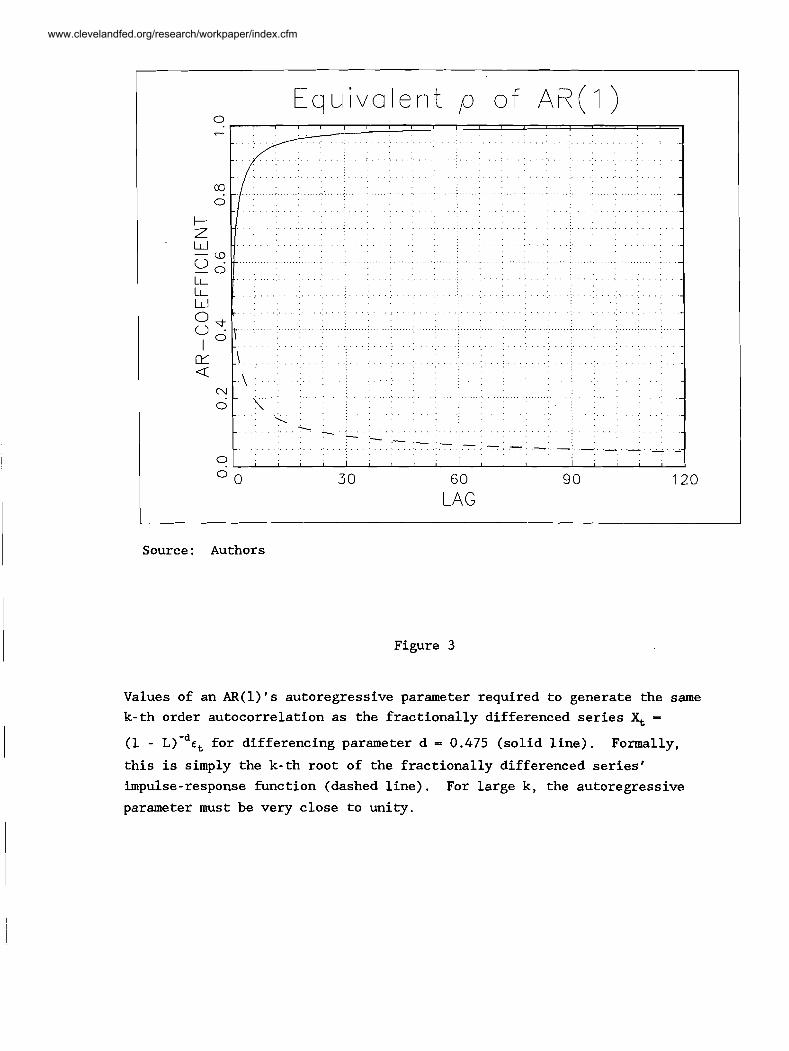
Figure 3

0

0

Values of an AR(1)'s autoregressive parameter required to generate the same

k-th order autocorrelation as the fractionally differenced series X, =

(1 - ~ ) - ~ e , for differencing parameter d = 0.475 (solid line). Formally,

this is simply the k-th root of the fractionally differenced series'

impulse-response function (dashed line). For large k, the autoregressive

parameter must be very close to unity.

. . . . . . . . . . . . . . . . . . . . . . . . w - : . : . : . . . . . . . . . . . . . . . . . . . . . . . . . . . . . . . '. . . . . . . . . . . . . . . . . . . . . . . . . . . . .

. . . . . . . . . . . . . . . . . . . ." ". . . . . . . . . . . . .

. . . . . . . . . . . . . . . . . . . . . . . . . . . . . . . . . . . . . . . . . . . . . . . . . . . . . . . . . . . . . . . . . . . . . . . . - . . . . . . . . . . . . . . - . .

. . . . . . . . . . . .

. . . . . . . . . . . . . . . . . . . . . . . . . . . . . . . . . . . . . . . . . . . . . . . . . . : . . . . . . - - < .: , ; . i . I . , ; .- . . . . - . . . . . . . . . . . . . - - . . . . . . . . . . . . . - . _ I _ _ . . . . . . . . . . . . . . . . . . . . . . . . . . . . . . . . . . . . . . . . . . . . . . . . . . . - . .- ,-.. .-. .&. . . , . - . . . . . . . . . . . . . . . . - - . . : . . . . . . . . . .

0 ~ " " 1 " " ~ " " 1 " " 30 60 90 120

LAG


Source : Authors

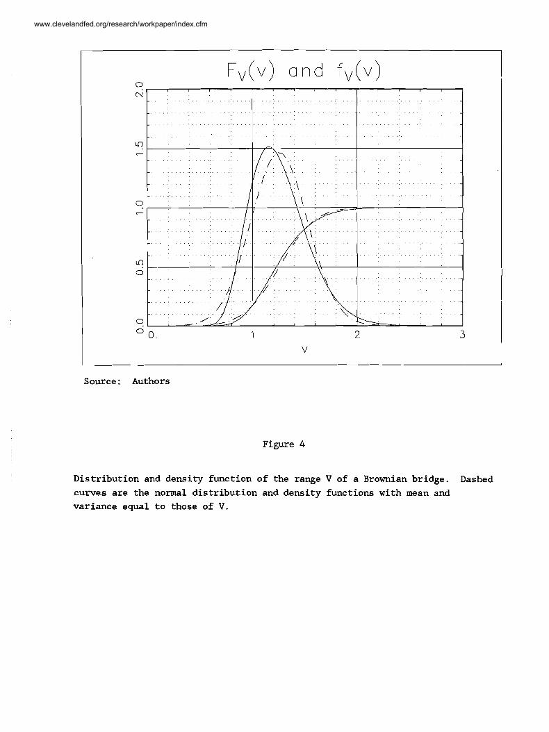
Figure 4

Distribution and density function of the range V of a Brownian bridge. Dashed

curves are the normal distribution and density functions with mean and

variance equal to those of V.


Table la. Fractiles of the Distribution Fv(v)

Table Ib. Symmetric Confidence Intervals about the Mean

Source: Authors


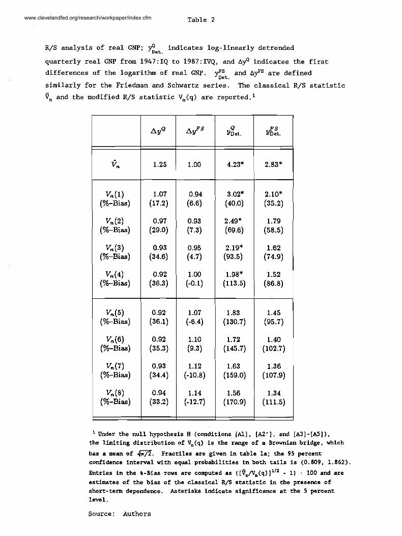
Table 2

R/S analysis of real GNP; . indicates log- linearly detrended

quarterly real GNP from 1947 : IQ to 1987 : IVQ, and indicates the first

differences of the logarithm of real GNP. g:. and AfS are defined

similarly for the Friedman and Schwartz series. The classical R/S statistic

9, and the modified R/S statistic Vn(q) are reported. l

Under the null hypothesis H (conditions [All , [A2 ' ] , and [A31 - [AS] ) , the limiting distribution of V,(q) is the range of a Brownian bridge, which

has a mean of m. Fractiles are given in table la; the 95 percent confidence interval with equal probabilities in both tails is (0.809, 1.862).

Entries in the %-Bias rows are computed as ([~,/v,(~)]"~ - 1) 100 and are

estimates of the bias of the classical R/S statistic in the presence of short-term dependence. Asterisks indicate significance at the 5 percent level.

Source : Authors


Table 3

Finite sample distribution of the modified R/S statistic under i.i.d. and ARMA(2,2) null hypotheses for the first difference of real log-GNP. The Monte Carlo experiments under the two null hypotheses are independent and consist of 10,000 replications each. Parameters of the i. i. d. simulations were chosen to match the sample mean and variance of quarterly real GNP growth rates from 1947:IQ to 1987:IVQ; parameters of the ARMA(2,2) were chosen to match point estimates of an ARMA(2,2) model fitted to the same data set. Entries in the column labeled "q" indicate the number of lags used to compute the R/S statistic. A lag of zero corresponds to Mandelbrot's classical R/S statistic, and a non-integer lag value corresponds to the average (across replications) lag value used according to Andrews' (1991) optimal lag formula. Standard errors for the empirical size may be computed using the usual normal

approximation; they are 9.95 x 2.18 x and 3.00 x for the 1, 5, and 10 percent tests, respectively.

i.i.d. Null Hypothesis:

ARMA(2,2) Null Hypothesis:

n

163

163

163 163 163 163 163 163 163 163

Source: Authors

Size 10%-Test

0.138

0.121

0.125 0.111 0.097 0.082 0.071 0.061 0.050 0.040

Q

0

1.5

1 2 3 4 5 6 7 8

Max

2.457

2.457

2.423 2.326 2.221 2.136 2.087 2.039 1.989 1.960

n

163

163

163 163 163 163 163 163 163 163

Min

0.522

0.525

0.533 0.564 0.602 0.641 0.645 0.636 0.648 0.657

Min

0.746

0.610

0.626 0.564 0.550 0.569 0.609 0.616 0.629 0.644

q

0

6.8

1 2 3 4 5 6 7 8

Mean

1.167

1.171

1.170 1.174 1.179 1 . 1.189 1.193 1.198 1.203

Max

3.649

2.200

3.027 2.625 2.412 2.294 2.241 2.181 2.109 2.035

S. D.

0.264

0.253

0.254 0.246 0.239 0.232 0.225 0.219 0.213 0.207

Mean

1.730

1.177

1.439 1.273 1.202 1.180 1.178 1.180 1.180 1.179

Size 1%-Test

0.022

0.015

0.016 0.011 0.009 0.006 0.004 0.002 0.000 0.000

Siee 5%-Test

0.081

0.069

0.069 0.058 0.046 0.036 0.030 0.024 0.018 0.015

S. D .

0.396

0.229

0.321 0.279 0.257 0.244 0.236 0.229 0.222 0.215

Size 1%-Test

0.175

0.009

0.034 0.010 0.012 0.012 0.010 0.008 0.006 0.005

Size 5%-Test

0.340

0.041

0.110 0.054 0.055 0.054 0.048 0.040 0.034 0.030

Size 10%-Test

0.442

0.OM

0.182 0.111 0.108 0.102 0.093 0.082 0.079 0.066


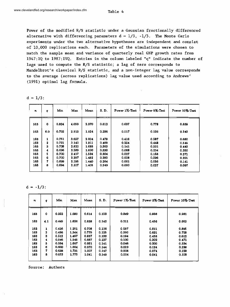
Table 4

Power of the modified R/S statistic under a Gaussian fractionally differenced alternative with differencing parameters d = 1/3, -1/3. The Monte Carlo experiments under the two alternative hypotheses are independent and consist of 10,000 replications each. Parameters of the simulations were chosen to

match the sample mean and variance of quarterly real GNP growth rates from 1947: IQ to 1987: IVQ. Entries in the column labeled "q" indicate the number of

lags used to compute the R/S statistic; a lag of zero corresponds to Mandelbrot's classical R/S statistic, and a non-integer lag value corresponds

to the average (across replications) lag value used according to Andrews'

(1991) optimal lag formula.

Source: Authors

n

163

163

163 163 163 163 163 163 163 163

Min

0.824

0.702

0.751 0.721 0.708 0.696 0.700 0.700 0.699 0.694

q

0

6.0

1 2 3 4 5 6 7 8

n

163

163

163 163 163 163 163 163 163 163

q

0

4.1

1 2 3 4 5 6 7 8

Min

0.352

0.449

0.416 0.466 0.512 0.546 0.564 0.600 0.658 0.652

Max

4.659

2.513

3.657 3.140 2.820 2.589 2.417 2.297 2.195 2.107

Max

1.080

1.626

1.251 1.344 1.467 1.545 1.667 1.664 1.731 1.775

Mean

2.370

1.524

2.004 1.811 1.688 1.600 1.534 1.482 1.440 1.405

Mean

0.614

0.838

0.708 0.779 0.837 0.887 0.931 0.970 1.007 1.041

S. D.

0.612

0.286

0.478 0.409 0.363 0.330 0.304 0.282 0.264 0.249

S. D.

0.103

0.142

0.116 0.125 0.132 0.137 0.141 0.144 0.147 0.149

Power 10%-Test

0.839

0.240

0.680 0.545 0.440 0.350 O.27l 0.201 0.141 0.097

Power 1%-Test

0.637

0.017

0.416 0.254 0.141 0.068 0.027 0.008 0.001 0.000

Power 1%-Teat

0.849

0.211

0.587 0.350 0.194 0.100 0.046 0.019 0.008 0.004

Power 5%-Test

0.778

0.126

0.587 0.448 0.331 0.234 0.158 0.096 0.056 0.027

Power 5%-Test

0.956

0.456

0.811 0.631 0.458 0.309 0.200 0.124 0.074 0.041

Power 10%-Test

0.981

0.600

0.895 0.758 0.612 0.47l 0.334 0.236 0.158 0.10s


the sources and nature of long-term memory in the business cycle

Documents