the solow model - karl · pdf fileuniversity college dublin, ma macroeconomics notes, 2014...
TRANSCRIPT

University College Dublin, MA Macroeconomics Notes, 2014 (Karl Whelan) Page 1
The Solow Model
We have discussed how economic growth can come from either capital deepening (increased
amounts of capital per worker) or from improvements in total factor productivity (sometimes
termed technological progress). This suggests that economic growth can come about from
saving and investment (so that the economy accumulates more capital) or from improvements
in productive efficiency. In these notes, we consider a model that explains the role these two el-
ements play in generating sustained economic growth. The model is also due to Robert Solow,
whose work on growth accounting we discussed in the last lecture, and was first presented in
his 1956 paper “A Contribution to the Theory of Economic Growth.”
The Solow Model’s Assumptions
The Solow model assumes that output is produced using a production function in which output
depends upon capital and labour inputs as well as a technological efficiency parameter, A.
Yt = AF (Kt, Lt) (1)
It is assumed that adding capital and labour raises output
∂Yt∂Kt
> 0 (2)
∂Yt∂Lt
> 0 (3)
However, the model also assumes there are diminishing marginal returns to capital accumula-
tion. In other words, adding extra amounts of capital gives progressively smaller and smaller
increases in output. This means the second derivative of output with respect to capital is
negative.
∂2Yt∂Kt
< 0 (4)
University College Dublin, MA Macroeconomics Notes, 2014 (Karl Whelan) Page 2
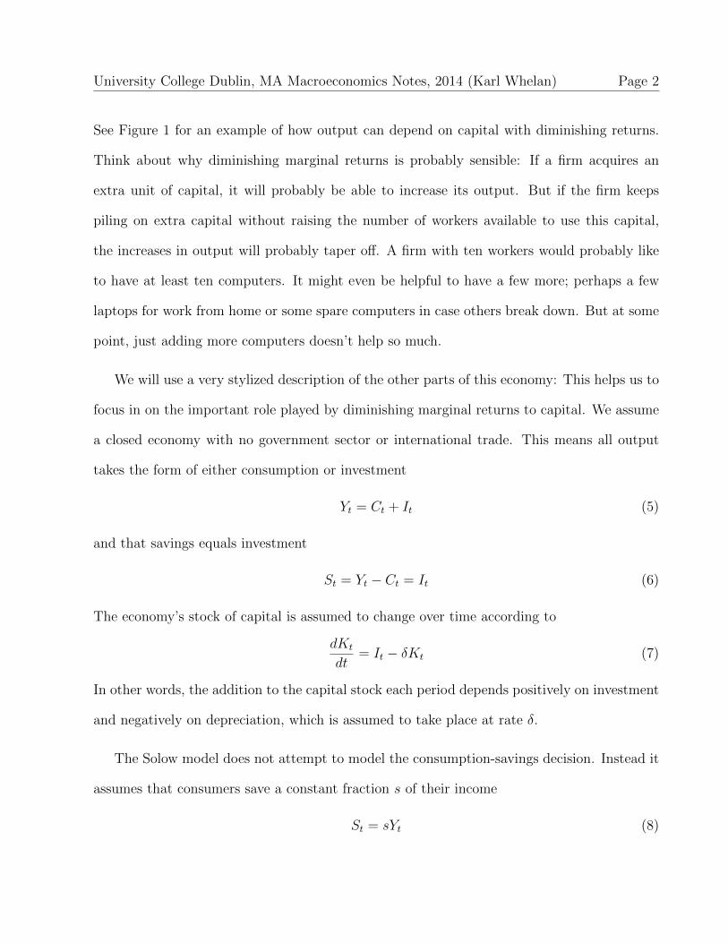
See Figure 1 for an example of how output can depend on capital with diminishing returns.
Think about why diminishing marginal returns is probably sensible: If a firm acquires an
extra unit of capital, it will probably be able to increase its output. But if the firm keeps
piling on extra capital without raising the number of workers available to use this capital,
the increases in output will probably taper off. A firm with ten workers would probably like
to have at least ten computers. It might even be helpful to have a few more; perhaps a few
laptops for work from home or some spare computers in case others break down. But at some
point, just adding more computers doesn’t help so much.
We will use a very stylized description of the other parts of this economy: This helps us to
focus in on the important role played by diminishing marginal returns to capital. We assume
a closed economy with no government sector or international trade. This means all output
takes the form of either consumption or investment
Yt = Ct + It (5)
and that savings equals investment
St = Yt − Ct = It (6)
The economy’s stock of capital is assumed to change over time according to
dKt
dt= It − δKt (7)
In other words, the addition to the capital stock each period depends positively on investment
and negatively on depreciation, which is assumed to take place at rate δ.
The Solow model does not attempt to model the consumption-savings decision. Instead it
assumes that consumers save a constant fraction s of their income
St = sYt (8)

University College Dublin, MA Macroeconomics Notes, 2014 (Karl Whelan) Page 3
Figure 1: Diminishing Marginal Returns to Capital
Capital
Output
Output
University College Dublin, MA Macroeconomics Notes, 2014 (Karl Whelan) Page 4
Capital Dynamics in the Solow Model
Because savings equals investment in the Solow model, equation (8) means that investment
is also a constant fraction of output
It = sYt (9)
which means we can re-state the equation for changes in the stock of capital
dKt
dt= sYt − δKt (10)
Whether the capital stock expands, contracts or stays the same depends on whether investment
is greater than, equal to or less than depreciation.
dKt
dt> 0 if δKt < sYt (11)
dKt
dt= 0 if δKt = sYt (12)
dKt
dt< 0 if δKt > sYt (13)
In other words, if the ratio of capital to output is such that
Kt
Yt=s
δ(14)
the the stock of capital will stay constant. If the capital-ouput ratio is lower than this level,
then the capital stock will be increasing and if it is higher than this level, it will be decreasing.
Figure 2 provides a graphical illustration of this process. Depreciation is a simple straight-
line function of the stock of capital while output is a curved function of capital, featuring
diminishing marginal returns. When the level of capital is low sYt is greater than δK. As
the capital stock increases, the additional investment due to the extra output tails off but the
additional depreciation does not, so at some point sYt equals δK and the stock of capital stops
increasing. Figure 2 labels the particular point at which the capital stock remains unchanged
as K∗. At this point, we have KtYt
= sδ.

University College Dublin, MA Macroeconomics Notes, 2014 (Karl Whelan) Page 5
In the same way, if we start out with a high stock of capital, then depreciation, δK, will
tend to be greater than investment, sYt. This means the stock of capital will decline. When
it reaches K∗ it will stop declining. This an example of what economists call convergent
dynamics. For any fixed set of the model parameters (s and δ) and other inputs into the
production (At and Lt) there will be a defined level of capital such that, no matter where the
capital stock starts, it will converge over time towards this level.
Figure 3 provides an illustration of how the convergent dynamics determine the level of
output in the Solow model. It shows output, investment and depreciation as a function of the
capital stock. The gap between the green line (investment) and the orange line (output) shows
the level of consumption. The economy converges towards the level of output associated with
the capital stock K∗.
An Increase in the Savings Rate
Now consider what happens when the economy has settled down at an equilibrium unchanging
level of capital K1 and then there is an increase in the savings rate from s1 to s2.
Figure 4 shows what happens to the dynamics of the capital stock. The line for investment
shifts upwards: For each level of capital, the level of output associated with it translates into
more investment. So the investment curve shifts up from the green line to the red line. Starting
at the initial level of capital, K1, investment now exceeds depreciation. This means the capital
stock starts to increase. This process continues until capital reaches its new equilibrium level
of K2 (where the red line for investment intersects with the black line for depreciation.) Figure
5 illustrates how output increases after this increase in the savings rate.

University College Dublin, MA Macroeconomics Notes, 2014 (Karl Whelan) Page 6
Figure 2: Capital Dynamics in The Solow Model
Capital, K
Investment,
Depreciation Depreciation δK
Investment sY
K*

University College Dublin, MA Macroeconomics Notes, 2014 (Karl Whelan) Page 7
Figure 3: Capital and Output in the Solow Model
Capital, K
Investment,
Depreciation,
Output
Depreciation δK
Investment sY
K*
Output Y
Consumption

University College Dublin, MA Macroeconomics Notes, 2014 (Karl Whelan) Page 8
Figure 4: An Increase in the Saving Rate
Capital, K
Investment,
Depreciation Depreciation δK
Old Investment s1Y
K1
New Investment s2Y
K2

University College Dublin, MA Macroeconomics Notes, 2014 (Karl Whelan) Page 9
Figure 5: Effect on Output of Increased Saving
Capital, K
Investment,
Depreciation
Output
Depreciation δK
Old Investment s1Y
K1
New Investment s2Y
K2
Output Y

University College Dublin, MA Macroeconomics Notes, 2014 (Karl Whelan) Page 10
An Increase in the Depreciation Rate
Now consider what happens when the economy has settled down at an equilibrium unchanging
level of capital K1 and then there is an increase in the depreciation rate from δ1 to δ2.
Figure 6 shows what happens in this case. The depreciation schedule shifts up from the
black line associated with the original depreciation rate, δ1, to the new red line associated with
the new depreciation rate, δ2. Starting at the initial level of capital, K1, depreciation now
exceeds investment. This means the capital stock starts to decline. This process continues
until capital falls to its new equilibrium level of K2 (where the red line for depreciation
intersects with the green line for investment.) So the increase in the depreciation rate leads
to a decline in the capital stock and in the level of output.
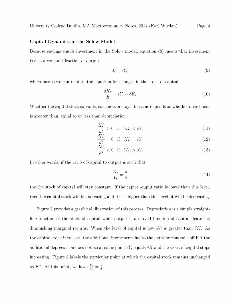
An Increase in Technological Efficiency
Now consider what happens when technological efficiency At increases. Because investment
is given by
It = sYt = sAF (Kt, Lt) (15)
a one-off increase in A thus has the same effect as a one-off increase in s. Capital and output
gradually rise to a new higher level. Figure 7 shows the increase in capital due to an increase
in technological efficiency.

University College Dublin, MA Macroeconomics Notes, 2014 (Karl Whelan) Page 11
Figure 6: An Increase in Depreciation
Capital, K
Investment,
Depreciation Old Depreciation δ1K
Investment sY
K1
K2
New Depreciation δ2K
University College Dublin, MA Macroeconomics Notes, 2014 (Karl Whelan) Page 12
Figure 7: An Increase in Technological Efficiency
Capital, K
Investment,
Depreciation
Depreciation δK
Old Technology A1F(K,L)
K1
New Technology A2F(K,L)
K2

University College Dublin, MA Macroeconomics Notes, 2014 (Karl Whelan) Page 13
Solow and the Sources of Growth
In the last lecture, we described how capital deepening and technological progress were the
two sources of growth in output per worker. Specifically, we derived an equation in which
output growth was a function of growth in the capital stock, growth in the number of workers
and growth in technological efficiency.
Our previous discussion had pointed out that a one-off increase in technological efficiency,
At, had the same effects as a one-off increase in the savings rate, s. However, there are
important differences between these two types of improvements. The Solow model predicts
that economies can only achieve a temporary boost to economic growth due to a once-off
increase in the savings rate. If they want to sustain economic growth through this approach,
then they will need to keep raising the savings rate. However, there are likely to be limits in
any economy to the fraction of output that can be allocated towards saving and investment,
particularly if it is a capitalist economy in which savings decisions are made by private citizens.
Unlike the savings rate, which will tend to have an upward limit, there is no particular
reason to believe that technological efficiency At has to have an upper limit. Indeed, growth
accounting studies tend to show steady improvements over time in At in most countries. Going
back to Young’s paper on Hong Kong and Singapore discussed in the last lecture, you can
see now why it matters whether an economy has grown due to capital deepening or TFP
growth. The Solow model predicts that a policy of encouraging growth through more capital
accumulation will tend to tail off over time producing a once-off increase in output per worker.
In contrast, a policy that promotes the growth rate of TFP can lead to a sustained higher
growth rate of output per worker.

University College Dublin, MA Macroeconomics Notes, 2014 (Karl Whelan) Page 14
The Capital-Output Ratio with Steady Growth
Up to now, we have only considered once-off changes in output. Here, however, we consider
how the capital stock behaves when the economy grows at steady constant rate GY . Specif-
ically, we can show in this case that the ratio of capital to output will tend to converge to a
specific value. Recall from the last lecture that if we have something of the form
Zt = Uαt W
βt (16)
then we have the following relationship between the various growth rates
GZt = αGU
t + βGWt (17)
The capital output ratio KtYt
can be written as KtY−1t . So the growth rate of the capital-output
ratio can be written as
GKYt = GK
t −GYt (18)
Adjusting equation 10, the growth rate of the capital stock can be written as
GKt =
1
Kt
dKt
dt= s
YtKt
− δ (19)
so the growth rate of the capital-output ratio is
GKYt = s
YtKt
− δ −GY (20)
This gives a slightly different form of convergence dynamics from those we saw earlier. This
equation shows that the growth rate of the capital-output ratio depends negatively on the
level of this ratio. This means the capital-output ratio displays convergent dynamics. When
it is above a specific equilibrium value it tends to fall and when it is below this equilibrium
value it tends to increase. Thus, the ratio is constantly moving towards this equilibrium value.
University College Dublin, MA Macroeconomics Notes, 2014 (Karl Whelan) Page 15
We can express this formally as follows:
GKYt > 0 if
Kt
Yt<
s
δ +GY(21)
GKYt = 0 if
Kt
Yt=
s
δ +GY(22)
GKYt < 0 if
Kt
Yt>
s
δ +GY(23)
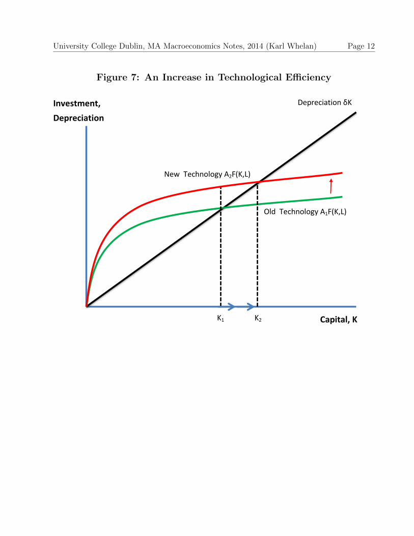
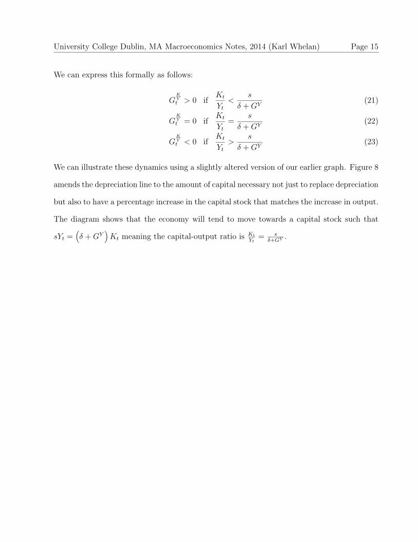
We can illustrate these dynamics using a slightly altered version of our earlier graph. Figure 8
amends the depreciation line to the amount of capital necessary not just to replace depreciation
but also to have a percentage increase in the capital stock that matches the increase in output.
The diagram shows that the economy will tend to move towards a capital stock such that
sYt =(δ +GY
)Kt meaning the capital-output ratio is Kt
Yt= s
δ+GY.

University College Dublin, MA Macroeconomics Notes, 2014 (Karl Whelan) Page 16
Figure 8: The Equilibrium Capital Stock in a Growing Economy
Capital, K
Investment,
Depreciation Depreciation and Growth (δ+GY)K
Investment sY
K*

University College Dublin, MA Macroeconomics Notes, 2014 (Karl Whelan) Page 17
Why Growth Accounting Can Be Misleading
Of the cases just considered in which output and capital both increase—an increase in the
savings rate and an increase in the level of TFP—the evidence points to increases in TFP
being more important as a generator of long-term growth. Rates of savings and investment
tend for most countries tend to stay within certain ranges while large increases in TFP over
time have been recorded for many countries. It’s worth noting then that growth accounting
studies can perhaps be a bit misleading when considering the ultimate sources of growth.
Consider a country that has a constant share of GDP allocated to investment but is
experiencing steady growth in TFP. The Solow model predicts that this economy should
experience steady increases in output per worker and increases in the capital stock. A growth
accounting exercise may conclude that a certain percentage of growth stems from capital
accumulation but ultimately, in this case, all growth (including the growth in the capital
stock) actually stems from growth in TFP. The moral here is that pure accounting exercises
may miss the ultimate cause of growth.

University College Dublin, MA Macroeconomics Notes, 2014 (Karl Whelan) Page 18
Krugman on “The Myth of Asia’s Miracle”
I encourage you to read Paul Krugman’s 1994 article “The Myth of Asia’s Miracle.” It
discusses a number of examples of cases where economies where growth was based on largely
on capital accumulation. In addition to the various Asian countries covered in Alwyn Young’s
research, Krugman (correctly) predicted a slowdown in growth in Japan, even though at the
time many US commentators were focused on the idea that Japan was going to overtake US
levels of GDP per capita.
Perhaps most interesting is his discussion of growth in the Soviet Union. Krugman notes
that the Soviet economy grew strongly after World War 2 and many in the West believed they
would become more prosperous than capitalist economies. The Soviet Union’s achievement
in placing the first man in space provoked Kennedy’s acceleration in the space programme,
mainly to show the U.S. was not falling behind communist systems. However, some economists
that had examined the Soviet economy were less impressed. Here’s an extended quote from
Krugman’s article:
When economists began to study the growth of the Soviet economy, they did so
using the tools of growth accounting. Of course, Soviet data posed some prob-
lems. Not only was it hard to piece together usable estimates of output and input
(Raymond Powell, a Yale professor, wrote that the job “in many ways resembled
an archaeological dig”), but there were philosophical difficulties as well. In a so-
cialist economy one could hardly measure capital input using market returns, so
researchers were forced to impute returns based on those in market economies at
similar levels of development. Still, when the efforts began, researchers were pretty
sure about what: they would find. Just as capitalist growth had been based on

University College Dublin, MA Macroeconomics Notes, 2014 (Karl Whelan) Page 19
growth in both inputs and efficiency, with efficiency the main source of rising per
capita income, they expected to find that rapid Soviet growth reflected both rapid
input growth and rapid growth in efficiency.
But what they actually found was that Soviet growth was based on rapid–growth
in inputs–end of story. The rate of efficiency growth was not only unspectacular,
it was well below the rates achieved in Western economies. Indeed, by some
estimates, it was virtually nonexistent.
The immense Soviet efforts to mobilize economic resources were hardly news. Stal-
inist planners had moved millions of workers from farms to cities, pushed millions
of women into the labor force and millions of men into longer hours, pursued mas-
sive programs of education, and above all plowed an ever-growing proportion of
the country’s industrial output back into the construction of new factories.
Still, the big surprise was that once one had taken the effects of these more or
less measurable inputs into account, there was nothing left to explain. The most
shocking thing about Soviet growth was its comprehensibility.
This comprehensibility implied two crucial conclusions. First, claims about the
superiority of planned over market economies turned out to be based on a mis-
apprehension. If the Soviet economy had a special strength, it was its ability to
mobilize resources, not its ability to use them efficiently. It was obvious to every-
one that the Soviet Union in 1960 was much less efficient than the United States.
The surprise was that it showed no signs of closing the gap.
Second, because input-driven growth is an inherently limited process, Soviet growth
was virtually certain to slow down. Long before the slowing of Soviet growth be-
University College Dublin, MA Macroeconomics Notes, 2014 (Karl Whelan) Page 20
came obvious, it was predicted on the basis of growth accounting.
The Soviet leadership did a good job for a long time of hiding from the world that their
economy had stopped growing but ultimately the economic failures of the centrally planning
model (combined with its many political and ethnic tensions) ended in a dramatic implosion
of the communist system in Russia and the rest of Eastern Europe.
A Formula for Steady Growth
All of the results so far apply for any production function with diminishing marginal returns
to capital. However, we can also derive some useful results by making specific assumptions
about the form of the production function. Specifically, we will consider the constant returns
to scale Cobb-Douglas production function
Yt = AtKαt L
1−αt (24)
This means output growth is determined by
GYt = GA
t + αGKt + (1 − α)GL
t (25)
Now consider the case in which the growth rate of labour input is fixed at n
GLt = n (26)
and the growth rate of total factor productivity is fixed at g.
GAt = g (27)
The formula for output growth becomes
GYt = g + αGK
t + (1 − α)n (28)

University College Dublin, MA Macroeconomics Notes, 2014 (Karl Whelan) Page 21
This means all variations in the growth rate of output are due to variations in the growth
rate for capital. If output is growing at a constant rate, then capital must also be growing at
a constant rate. And we know that the capital-output ratio tends to move towards a specific
equilibrium value. So along a steady growth path, the growth rate of output equals the growth
rate of capital. Thus, the previous equation can be re-written
GYt = g + αGY
t + (1 − α)n (29)
which can be simplified to
GYt =
g
1 − α+ n (30)
The growth rate of output per worker is
GYt − n =
g
1 − α(31)
So the economy tends to converge towards a steady growth path and the growth rate of output
per worker along this path is g1−α . Without growth in technological efficiency, there can be
no steady growth in output per worker.
A Useful Formula for Output Per Worker
In this case of the Cobb-Douglas production function, output per worker can be written as
YtLt
= At
(Kt
Lt
)α(32)
In other words, output per worker is a function of technology and of capital per worker. A
drawback of this representation is that we know that increases in At also increase capital
per worker, so this has the misleading implications about the role of capital accumulation
discussed above. It is useful, then, to derive an alternative characterisation of output per
University College Dublin, MA Macroeconomics Notes, 2014 (Karl Whelan) Page 22
worker, one that we will use again. First, we’ll define the capital-output ratio as
xt =Kt
Yt(33)
So, the production function can be expressed as
Yt = At (xtYt)α L1−α
t (34)
Here, we are using the fact that
Kt = xtYt (35)
Dividing both sides of this expression by Y αt , we get
Y 1−αt = Atx
αt L
1−αt (36)
Taking both sides of the equation to the power of 11−α we arrive at
Yt = A1
1−αt x
α1−αt Lt (37)
So, output per worker is
YtLt
= A1
1−αt x
α1−αt (38)
This equation states that all fluctuations in output per worker are due to either changes in
technological progress or changes in the capital-output ratio. When considering the relative
role of technological progress or policies to encourage accumulation, we will see that this
decomposition is more useful than equation (32) because the level of technology does not
affect xt in the long run while it does affect KtLt
. So, this decomposition offers a cleaner picture
of the part of growth due to technology and the part that is not.
University College Dublin, MA Macroeconomics Notes, 2014 (Karl Whelan) Page 23
A Formal Model of Convergence Dynamics
Because At is assumed to grow at a constant rate each period, this means that all of the
interesting dynamics for output per worker in this model stem from the behaviour of the
capital-output ratio. We will now describe in more detail how this ratio behaves. Before
doing so, I want to introduce a new piece of terminology that we will use in the next few
lectures.
A useful mathematical shorthand that saves us from having to write down derivatives with
respect to time everywhere is to write
Yt =dYtdt
(39)
What we are really interested in, though, is growth rates of series, so we need to scale this by
the level of output itself. Thus, YtYt
, and this is our mathematical expression for the growth
rate of a series. For our Cobb-Douglas production function, we can use the result we derived
earlier to express the growth rate of output as
YtYt
=AtAt
+ αKt
Kt
+ (1 − α)LtLt
(40)
The Solow model assumes
AtAt
= g (41)
Nt
Nt
= n (42)
So this can be re-written as
YtYt
= g + αKt
Kt
+ (1 − α)n (43)
Similarly, because
xt = KtYt−1 (44)
University College Dublin, MA Macroeconomics Notes, 2014 (Karl Whelan) Page 24
its growth rate can be written as
xtxt
=Kt
Kt
− YtYt
(45)
To get an expression for the growth rate of the capital stock, w re-write the capital accu-
mulation equation as
Kt = sYt − δKt (46)
and divide across by Kt on both sides
Kt
Kt
= sYtKt
− δ (47)
This means we write, the growth rate of the capital stock as
Kt
Kt
=s
xt− δ (48)
Now using equation (43) for output growth and equation (48) for capital growth, we can
derive a useful equation for the dynamics of the capital-output ratio:
xtxt
= (1 − α)Kt
Kt
− g − (1 − α)n (49)
= (1 − α)(s
xt− g
1 − α− n− δ) (50)
This dynamic equation has a very important property: The growth rate of xt depends nega-
tively on the value of xt. In particular, when xt is over a certain value, it will tend to decline,
and when it is under that value it will tend to increase. This provides a specific illustration
of the convergent dynamics of the capital-output ratio.
What is the long-run steady-state value of xt, which we will label x∗? It is the value
consistent with xx
= 0. This implies that
s
x∗− g
1 − α− n− δ = 0 (51)

University College Dublin, MA Macroeconomics Notes, 2014 (Karl Whelan) Page 25
This solves to give
x∗ =s
g1−α + n+ δ
(52)
Given this equation, we can derive a more intuitive-looking expression to describe the conver-
gence properties of the capital-output ratio. The dynamics of xt are given by
xtxt
= (1 − α)(s
xt− g
1 − α− n− δ) (53)
Multiplying and dividing the right-hand-side of this equation by ( g1−α + n+ δ):
xtxt
= (1 − α)(g
1 − α+ n+ δ)
(s/xt − g
1−α − n− δg
1−α + n+ δ
)(54)
The last term inside the brackets can be simplified to give
xtxt
= (1 − α)(g
1 − α+ n+ δ)
(1
xt
sg
1−α + n+ δ− 1
)(55)
= (1 − α)(g
1 − α+ n+ δ)
(x∗
xt− 1
)(56)
= (1 − α)(g
1 − α+ n+ δ)
(x∗ − xtxt
)(57)
This equation states that each period the capital-output ratio closes a fraction equal to λ =
(1 − α)( g1−α + n + δ) of the gap between the current value of the ratio and its steady-state
value.
Illustrating Convergence Dynamics
Often, the best way to understand dynamic models is to load them onto the computer and
see them run. This is easily done using spreadsheet software such as Excel or econometrics-
oriented packages such as RATS. Figures 1 to 3 provide examples of the behaviour over time
of two economies, one that starts with a capital-output ratio that is half the steady-state level,
and other that starts with a capital output ratio that is 1.5 times the steady-state level.

University College Dublin, MA Macroeconomics Notes, 2014 (Karl Whelan) Page 26
The parameters chosen were s = 0.2, α = 13, g = 0.02, n = 0.01, δ = 0.06. Together these
parameters are consistent with a steady-state capital-output ratio of 2. To see, this plug these
values into (52):
x∗ =(K
Y
)∗=
sg
1−α + n+ δ=
0.2
1.5 ∗ 0.02 + 0.01 + 0.06= 2 (58)
Figure 9 shows how the two capital-output ratios converge, somewhat slowly, over time to
their steady-state level. This slow convergence is dictated by our choice of parameters: Our
“convergence speed” is:
λ = (1 − α)(g
1 − α+ n+ δ) =
2
3(1.5 ∗ 0.02 + 0.01 + 0.06) = 0.067 (59)
So, the capital-output ratio converges to its steady-state level at a rate of about 7 percent
per period. These are fairly standard parameter values for annual data, so this should be
understood to mean 7 percent per year.
Figure 10 shows how output per worker evolves over time in these two economies. Both
economies exhibit growth, but the capital-poor economy grows faster during the convergence
period than the capital-rich economy. These output per worker differentials may seem a little
small on this chart, but the Figure 11 shows the behaviour of the growth rates, and this chart
makes it clear that the convergence dynamics can produce substantially different growth rates
depending on whether an economy is above or below its steady-state capital-output ratio.
During the initial transition periods, the capital-poor economy grows at rates over 6 percent,
while the capital-rich economy grows at under 2 percent. Over time, both economies converge
towards the steady-state growth rate of 3 percent.

University College Dublin, MA Macroeconomics Notes, 2014 (Karl Whelan) Page 27
Figure 9: Convergence Dynamics for the Capital-Output Ratio

University College Dublin, MA Macroeconomics Notes, 2014 (Karl Whelan) Page 28
Figure 10: Convergence Dynamics for Output Per Worker

University College Dublin, MA Macroeconomics Notes, 2014 (Karl Whelan) Page 29
Figure 11: Convergence Dynamics for the Growth Rate of Output Per Worker

University College Dublin, MA Macroeconomics Notes, 2014 (Karl Whelan) Page 30
Illustrating Changes in Key Parameters
Figures 12 to 14 examine what happens when the economy is moving along the steady-state
path consistent with the parameters just given, and then one of the parameters is changed.
Specifically, they examine the effects of changes in s, δ and g.
Consider first an increase in the savings rate to s = 0.25. This has no effect on the
steady-state growth rate. But it does change the steady-state capital-output ratio from 2 to
2.5. So the economy now finds itself with too little capital relative to its new steady-state
capital-output ratio. The growth rate jumps immediately and only slowly returns to the long-
run 3 percent value. The faster pace of investment during this period gradually brings the
capital-output ratio into line with its new steady-state level.
The increase in the savings rate permanently raises the level of output per worker relative
to the path that would have occurred without the change. However, for our parameter values,
this effect is not that big. This is because the long-run effect of the savings rate on output per
worker is determined by sα
1−α , which in this case is s0.5. So in our case, 25 percent increase in
the savings rate produces an 11.8 percent increase in output per worker (1.250.5 = 1.118). More
generally, a doubling of the savings rate raises output per worker by 41 percent (20.5 = 1.41).
The charts also show the effect of an increase in the depreciation rate to δ = 0.11. This
reduces the steady-state capital-output ratio to 4/3 and the effects of this change are basically
the opposite of the effects of the increase in the savings rate.
Finally, there is the increase in the rate of technological progress. I’ve shown the effects of
a change from g = 0.02 to g = 0.03. This increases the steady-state growth rate of output per
worker to 0.045. However, as the charts show there is another effect: A faster steady-state
growth rate for output reduces the steady-state capital-output ratio. Why? The increase in

University College Dublin, MA Macroeconomics Notes, 2014 (Karl Whelan) Page 31
g raises the long-run growth rate of output; this means that each period the economy needs
to accumulate more capital than before just to keep the capital-output ratio constant. Again,
without a change in the savings rate that causes this to happen, the capital-output ratio will
decline. So, the increase in g means that—as in the depreciation rate example—the economy
starts out in period 25 with too much capital relative to its new steady-state capital-output
ratio. For this reason, the economy doesn’t jump straight to its new 4.5 percent growth rate
of output per worker. Instead, after an initial jump in the growth rate, there is a very gradual
transition the rest of the way to the 4.5 percent growth rate.

University College Dublin, MA Macroeconomics Notes, 2014 (Karl Whelan) Page 32
Figure 12: Capital-Output Ratios: Effect of Increases In ...

University College Dublin, MA Macroeconomics Notes, 2014 (Karl Whelan) Page 33
Figure 13: Growth Rates of Output Per Hour: Effect of Increases In ...

University College Dublin, MA Macroeconomics Notes, 2014 (Karl Whelan) Page 34
Figure 14: Output Per Hour: Effect of Increases In ...

University College Dublin, MA Macroeconomics Notes, 2014 (Karl Whelan) Page 35
Convergence Dynamics in Practice
The Solow model predicts that no matter what the original level of capital an economy starts
out with, it will tend to revert to the equilibrium levels of output and capital indicated by
the economy’s underlying features. Does the evidence support this idea?
Unfortunately, history has provided a number of extreme examples of economies having
far less capital than is consistent with their fundamental features. Wars have provided the
“natural experiments” in which various countries have had huge amounts of their capital
destroyed. The evidence has generally supported Solow’s prediction that economies that
experience negative shocks should tend to recover from these setbacks and return to their
pre-shock levels of capital and output. For example, both Germany and Japan grew very
strongly after the war, recovering prosperity despite the massive damage done to their stocks
of capital by war bombing.
A more extreme example, perhaps, is study by Edward Miguel and Gerard Roland of the
long-run impact of U.S. bombing of Vietnam in the 1960s and 1970s. Miguel and Roland found
large variations in the extent of bombing across the various regions of Vietnam. Despite large
differences in the extent of damage inflicted on different regions, Miguel and Roland found
little evidence for lasting relative damage on the most-bombed regions by 2002. (Note this
is not the same as saying there was no damage to the economy as a whole — the study is
focusing on whether those areas that lost more capital than average ended up being poorer
than average).

University College Dublin, MA Macroeconomics Notes, 2014 (Karl Whelan) Page 36
Things to Understand from these Notes
Here’s a brief summary of the things that you need to understand from these notes.
1. The assumptions of the Solow model.
2. The rationale for diminishing marginal returns to capital accumulation.
3. Effects of changes in savings rate, depreciation rate and technology in the Solow model.
4. Why technological progress is the source of most growth.
5. Why growth accounting calculations can underestimate the role of technological progress.
6. Krugman on the Soviet Union.
7. The Solow model’s predictions about convergent dynamics.
8. The formula for steady growth rate with a Cobb-Douglas production function.
9. The formula for the convergence rate with a Cobb-Douglas production function.
10. Historical examples of convergent dynamics.