THE S

OLAR W

IND’S

EFFECT

ON MUON F

LUX

F I NA

L PR

ES

EN

T AT

I ON

BY

DA

VI D

RA

TH

MA

NN

- BL O

CH

Image Source: BBC

1

ABSTRACT

This experiment sought to evaluate the impact of the solar wind on the amount of muons coming in by correlating the rate of muon flux detected in a Quarknet 6000-series Scintillator detector with a) the natural day-night cycle an b) the dynamic solar wind data from NASA's SOHO satellite.

Using two different experimental setups (each running for 64 hours), the experimenter observed no statistically significant correlation between the day-night cycle and the rate of muon flux. He did, however, observe a seemingly statistically significant positive correlation between the muon flux and the real-time solar wind data; nevertheless, that correlation was neither linear nor completely supported by the data. On the setup with the detectors stacked atop one another and pointing directly up at the sky, a stronger visual correlation was observed (71% of data points within one standard deviation; 94% within two). When the Pearson Equation was used to find a correlation, it gave a value of about 0.44 (2 significant figures), which shows a mild positive correlation. On the setup with the detectors separated by a box and pointed toward the ecliptic, the visual correlation was not well shown (65% within one standard deviation; 88% within two). The Pearson value on the second data run showed a very, very weak negative correlation of -0.12.

Thus, this experiment showed no visible correlation between the day/night cycle and the muon flux. Using all four detectors stacked directly atop one another, it showed a mild positive correlation between the solar wind density and the measured muon flux. Using all four detectors, pointed toward the ecliptic, with a box in between them, the experiment showed no statistically significant correlation.

2Image Source: DeviantArt (users: Nightangel/Monoxism)

FOCUS QUESTIONS

1. How does the rate at which muons and other particles arrive change over time?

2. What does that demonstrate about the effects of the solar wind?

3. What significance does this have in a greater context?

Image Source: Daniel Wilkinson

3

BACKGROUND RESEARCH

Experiments similar to this one have, indeed, been completed in the past.

“Measurements of the Cosmic Muon Flux with the Willi Detector as a Source of Information about Solar Events” (Bucharest, 2010) found that there was approximately a 5% increase in muons during the day.

“Solar Wind Effect on the Muon Flux at Sea Level” (Rio De Janeiro, 2005) found that “Forbush events” in which the sun ejects plasma, and the muon flux is decreased, are common. Thus, solar events can sometimes be negatively correlated with muon flux.

4Image Source: Creative Commons (User: Originalwana)

SOLAR WIND: A QUOTIDIAN (DAILY) PATTERN?

• Initially, this experiment will compare muon flux during the day and at night. I will associate these day and night fluctuations with the solar wind by the following assumptions.

• In some cases, it takes particles from the solar wind many days to reach the earth.

• However, I think that those particles likely to affect my muon count will almost certainly be traveling closer to the speed of light; ergo, there will only be eight to ten minutes of delay between solar events and local events.

• Furthermore, for those particles most likely to result in muon production (or for those most likely to interfere with muon flux), it is reasonable for me to assume that, during the night, the earth’s large mass will prevent them from reaching my detector.

5Image Source: Zastavski.com

HYPOTHESIS

1. When the experiment is run, slightly more muons will likely be detected during the day, because some of them come from the solar wind. During the night, the earth will probably shield the detectors from those muons, so the muon flux (rate of arrival) will decrease slightly.

However, it’s also possible that the opposite will occur: more muons may be detected at night due to a decrease in solar wind modulation of the cosmic ray spectrum.

Image Source: collidingparticles.com

6

HYPOTHESIS (CONTINUED)

2. If the initial portion of my hypothesis (as well as my assumptions) is correct, a fair conclusion should be that the solar wind bolsters, rather than attenuates, the rate of muon flux.

3. If the first two components of my hypothesis are correct, I can conclude that the solar wind consists partially of particles that end up creating muons, because the modulation effect is well known and would reduce the rate of muon flux, were it the only variable in play.

Image Source: collidingparticles.com

7

After plateauing the four scintillators connected to a Quarknet DAQ board, I measure the muon flux by looking at the times when all four detectors are triggered simultaneously (within 40 ns of each other).

EXPERIMENTAL TECHNIQUE OVERVIEW

Image Source: Fermilab 8

DETAILED SETUP, 1ST EXPERIMENT

1) Without plugging the DAQ into a power source, connect all four scintillators’ data cables into the DAQ. Then, plug their power cables into the voltage regulator.  

2) Plug the voltage regulator cable into the DAQ. Then, plug a CAT5 cable into your GPS receiver and your DAQ’s GPS IN port.

3) Plug the USB (type B) connector into the DAQ and into a PC. You may need to install the CP210x Serial-to-USB driver on your PC.

4) Finally, after ensuring that each connection is tight, plug your DAQ into an electric outlet.

5) Start hyperterminal on your PC, and set up a new connection. Call it COM-3, use the port “COM3” and set the Bits per second to 115200. Finally, set the flow control to XON/XOFF.

6) Ensure that the scintillators are stacked on top of one another in order, and properly plateaued (see Quarknet’s Plateauing guidelines for more details). There should be no more than four centimeters between detectors, and they should be flat, facing up.

7) Run a short test at 4 coincidences. You should get approximately 5-8 counts per second, or 400-600 per minute (WC 00 3F ; 0.770 V in daytime).

8) Ensure other variables (time delay, threshold voltage, etc.) are set to their defaults for the Quarknet 6000 DAQ.

9Image Source: NASA

DETAILED PROCEDURE OF BOTH EXPERIMENTS

1) Prepare experimental equipment, as discussed in previous slide (or, for second experiment, on slides eighteen and nineteen).

2) Set up DAQ board to take data over a 24-hour (or longer) period. It should be counting four coincidences on all four stacked detectors (WC 00 3F via the COM/USB interface; http://quarknet.fnal.gov/toolkits/ati/det-user.pdf for assistance).

3) Capture the text data using the Quarknet guidelines.

4)  After 64 hours, finish the data collection, following the Quarknet guidelines. Run a Flux analysis.

5) From this raw data, make a more detailed result and propose an explanation (e.g., muon flux was 5% higher during the day, perhaps because some muons came from the solar wind).

6) Attempt to identify trends in the data. Also, check to see if the data correlate with real-time measurements of the solar wind using a visual standard deviation test and a Pearson (PPMCC) statistical correlation test.

7) Document findings, procedures, and potential sources of error.

10Image Source: NASA

0.55 0.6 0.65 0.7 0.75 0.8 0.85 0.9 0.95 1 1.050

2

4

6

8

10

12

14

16

18

Plateauing for all 4 coin-cidences

Voltage (V)

Counts (Hz)

PLAT

EAUIN

G DAT

A

To reduce noise and ensure the detectors’ functionality, I plateau the detectors by adjusting their voltage and comparing it to the count rate.

Plateau occurs around 0.80 V

11 Image Source: Sydney Electrical Contractors

PRELIM

INARY

RESULT

S

12

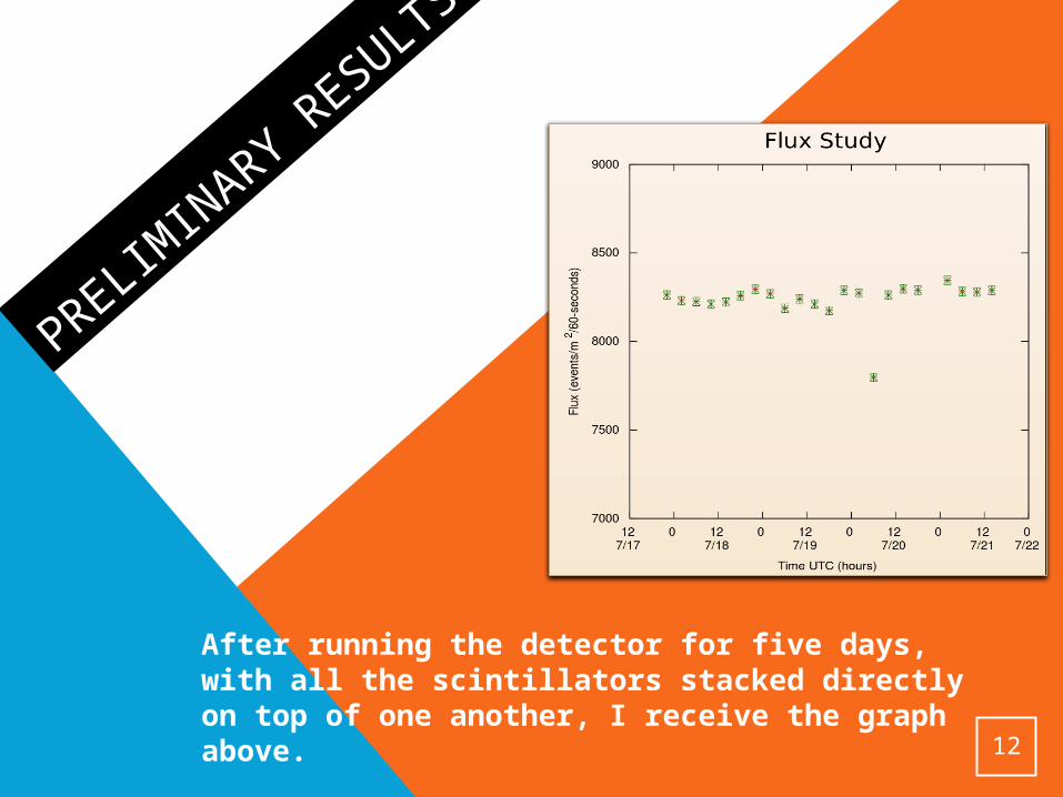
After running the detector for five days, with all the scintillators stacked directly on top of one another, I receive the graph above.

INTERPRETING MY PRELIMINARY RESULTS

Peaks

Outlier!

Irregular Curve

What do these data tell us?

No discernible daily pattern.

Fluctuations are generally not terribly statistically significant, at least with a bin width of four hours (1-3 error bars)

Further investigation is needed!

13

INTERPRETING RESULTS (CONTINUED)

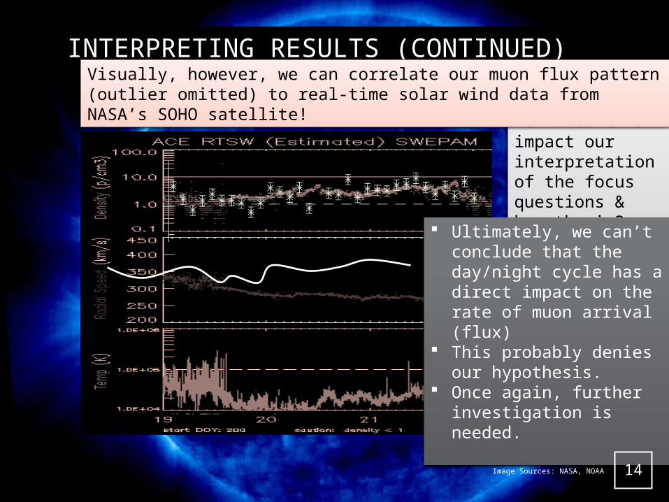
How does this impact our interpretation of the focus questions & hypothesis? Ultimately, we can’t

conclude that the day/night cycle has a direct impact on the rate of muon arrival (flux)

This probably denies our hypothesis.

Once again, further investigation is needed.

14

Visually, however, we can correlate our muon flux pattern (outlier omitted) to real-time solar wind data from NASA’s SOHO satellite!

Image Sources: NASA, NOAA

NOTES ON MY DATA FITOf course, this graph was not produced without a few statistical adjustments (see below).With these adjustments, 23 of my 32 (71%) 2-hour averages appear to be within one standard deviation of the SOHO data. Seven are within two standard deviations. Only two lie outside two standard deviations.

15

Proton density is measured logarithmically

But muon flux’s y-axis is measured linearly, from a flux of 8100 to 8600 events/m2/minute.

The scale is also offset by one hour, because these protons take longer to reach the earth than the satellite

PEARSON TEST OF STATISTICAL CORRELATION

We can calculate the degree of similarity between the two data sets by comparing the expected correlation (none) with the observed correlation. An R-value substantially greater than zero means a positive correlation; an R-value substantially less than zero means a negative correlation.

=

16Equaion source: Wikipedia

Bottom 122 107

Avg 91.35714286 92.42857143

PPMCC Value 2558

1 77 95 91.35714286 92.42857143 -14.35714286 2.571428571 -36.91836735 206.127551 6.612244898

2 99 96 91.35714286 92.42857143 7.642857143 3.571428571 27.29591837 58.41326531 12.75510204

3 118 99 91.35714286 92.42857143 26.64285714 6.571428571 175.0816327 709.8418367 43.18367347

4 103 105 91.35714286 92.42857143 11.64285714 12.57142857 146.3673469 135.5561224 158.0408163

5 93 104 91.35714286 92.42857143 1.642857143 11.57142857 19.01020408 2.698979592 133.8979592

6 100 104 91.35714286 92.42857143 8.642857143 11.57142857 100.0102041 74.69897959 133.8979592

7 106 97 91.35714286 92.42857143 14.64285714 4.571428571 66.93877551 214.4132653 20.89795918

8 122 105 91.35714286 92.42857143 30.64285714 12.57142857 385.2244898 938.9846939 158.0408163

9 107 101 91.35714286 92.42857143 15.64285714 8.571428571 134.0816327 244.6989796 73.46938776

10 82 94 91.35714286 92.42857143 -9.357142857 1.571428571 -14.70408163 87.55612245 2.469387755

11 117 86 91.35714286 92.42857143 25.64285714 -6.428571429 -164.8469388 657.5561224 41.32653061

12 91 91 91.35714286 92.42857143 -0.357142857 -1.428571429 0.510204082 0.12755102 2.040816327

13 94 92 91.35714286 92.42857143 2.642857143 -0.428571429 -1.132653061 6.984693878 0.183673469

14 66 89 91.35714286 92.42857143 -25.35714286 -3.428571429 86.93877551 642.9846939 11.75510204

15 97 95 91.35714286 92.42857143 5.642857143 2.571428571 14.51020408 31.84183673 6.612244898

16 84 94 91.35714286 92.42857143 -7.357142857 1.571428571 -11.56122449 54.12755102 2.469387755

17 87 87 91.35714286 92.42857143 -4.357142857 -5.428571429 23.65306122 18.98469388 29.46938776

18 89 89 91.35714286 92.42857143 -2.357142857 -3.428571429 8.081632653 5.556122449 11.75510204

19 78 84 91.35714286 92.42857143 -13.35714286 -8.428571429 112.5816327 178.4132653 71.04081633

20 75 81 91.35714286 92.42857143 -16.35714286 -11.42857143 186.9387755 267.5561224 130.6122449

21 66 83 91.35714286 92.42857143 -25.35714286 -9.428571429 239.0816327 642.9846939 88.89795918

22 82 85 91.35714286 92.42857143 -9.357142857 -7.428571429 69.51020408 87.55612245 55.18367347

23 94 84 91.35714286 92.42857143 2.642857143 -8.428571429 -22.2755102 6.984693878 71.04081633

24 80 82 91.35714286 92.42857143 -11.35714286 -10.42857143 118.4387755 128.9846939 108.755102

25 97 72 91.35714286 92.42857143 5.642857143 -20.42857143 -115.2755102 31.84183673 417.3265306

26 72 96 91.35714286 92.42857143 -19.35714286 3.571428571 -69.13265306 374.6989796 12.75510204

27 100 100 91.35714286 92.42857143 8.642857143 7.571428571 65.43877551 74.69897959 57.32653061

28 82 98 91.35714286 92.42857143 -9.357142857 5.571428571 -52.13265306 87.55612245 31.04081633

29 91.35714286 92.42857143 0 0 0

30 91.35714286 92.42857143 0 0 0

31 91.35714286 92.42857143 0 0 0

32 91.35714286 92.42857143 0 0 0

91.35714286 92.42857143 91.35714286 92.42857143 0 0 0 0

Total sum 1491.714286 5972.428571 1892.857143

Sqrt(total sum) 77.28148919 43.50697809

Denominator 3362.284057

Final result 0.443660994

INTERPRETING THE PEARSON VALUE17

Image Source: “Skbekas”

• Putting all of the data into the Pearson equation, I receive a value of approximately 0.44. For my sample size (thousands of points; only 32 bins), I think this means that there is a statistically significant correlation between the two data sets.

A PARADIG

MATIC

SHIFT IN

MY

HYPOTH

ESIS

18

The

initi

al as

sum

ptions I

mad

e when

star

ting th

e ex

perim

ent a

re p

robab

ly

inco

rrect

!

•I a

ssum

ed th

at d

ay a

nd nig

ht var

iatio

ns

in h

igh-e

nergy

solar

win

d wou

ld b

e m

ore

impor

tant t

han ch

anges

in o

vera

ll sola

r

wind d

ensit

y.

•By

corre

latin

g my

resu

lts w

ith th

e

mea

sure

men

ts o

f the

SOHO sate

llite,

I

can se

e th

at th

e pro

ton d

ensit

y of

the

solar

win

d in sp

ace

seem

s to

pre

dict

chan

ges in

terre

stria

l muon

flux.

Image Source: NASA

ALTERING THE PROCEDURE

• Experimental changes may add precision to my data and thus make it easier to confirm the observed trend in a second data run. • It’s possible that orienting the detectors directly toward

the ecliptic will de-munge (reveal the true patterns in) the data. By placing the detectors further apart, and pointing them at the ecliptic (72 degrees in July), I’ll be able to reduce the solid angle of the sky and reduce the disparity in terms of units and scale between the two data sets. This may also increase my R-value from the PPMCC test, helping confirm my correlation; or, it could make a false correlation disappear.

Image Source: collidingparticles.com

19

EXPERIMENTAL SETUP, SECOND EDITION

Image Source: collidingparticles.com

Top scintillator

Central box to reduce solid angle

Angle of 72 degrees to point toward ecliptic.

20

Box height = 21 cm

SECOND RUN R

ESULTS

21

After running the detector for three days, with all the scintillators stacked according to the 2nd Edition Experimental Setup, I receive the graph above. It also shows no day/night cycle.

INTERPRETING RESULTS – 2ND EXPERIMENT

22

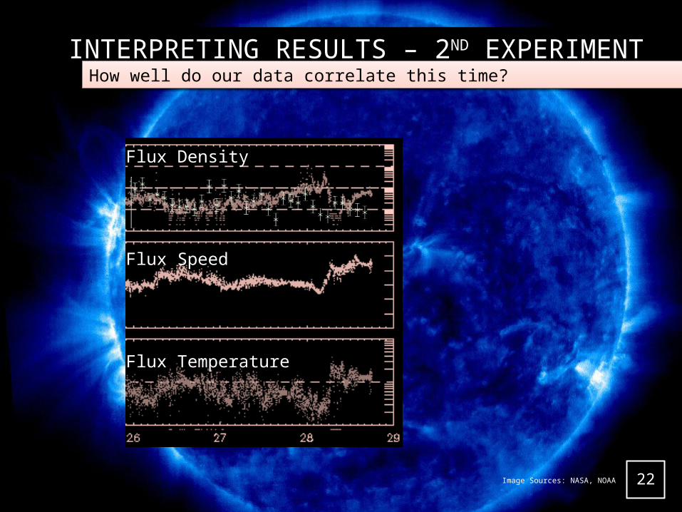
How well do our data correlate this time?

Image Sources: NASA, NOAA

Flux Density

Flux Speed

Flux Temperature

NOTES ON MY 2ND DATA FITThe data do not seem to support as strong a correlation this time.

Visually, my adjusted data gives the following conclusions: 21 of my 32 (66%) 2-hour averages appear to be within one standard deviation of the SOHO data; seven are within two standard deviations; and four lie outside two standard deviations.

Once again, this graph was not produced without a few statistical adjustments (see below).

23

Proton density is measured logarithmically (same scale as before)

But muon flux’s y-axis is measured linearly, from a flux of 2600 to 2750 events/m2/minute. (Yes, the flux went down.)

The scale is offset once again by one hour, because these protons take longer to reach the earth than the satellite

PEARSON TEST, 2ND EXPERIMENT

= on the data set gives us a value of about -0.12, which is not all that statistically significant for my sample size, and definitely does not indicate a positive correlation. It could indicate a very, very slight negative correlation.

24

Image Source: “Skbekas”

A DISPARITY

BETWEEN TWO

TECHNIQUES?

25

The second experiment (euphemistically) doesn’t look as well correlated as the first did.• It’s possible that the first result was unusual and that a

re-run of the first experiment would not indicate a correlation with the solar wind density.

• It’s also possible that the second half of the second experiment was atypical due to unexplained phenomena.

• It’s possible that poorly controlled variables in the second experiment impacted the results. From a visual inspection, the experimental setup may have sagged by about 2 cm over time, which could have put the detectors out of alignment and caused the steady downward trend in flux during the second half of the data run. I wasn’t able to verify if that occurred or not.

• In the second experiment, increasing the distance between detectors reduced the overall flux by about 2/3; it likely reduced the signal-to-noise ratio by that amount.

Image Source: NASA

FURTHER RESEARCH

This experiment’s conclusion is not terribly strong: a correlation observed using one experimental technique disappeared when the technique was altered. If I had more time and resources, I would do more data runs using the first experimental setup to see if the correlation observed was a statistical blip or whether it was a consistent finding. Then, I would do more data runs using the second experimental setup (but perhaps one manufactured to greater precision) to see if I could verify the disparity between the two setups.

26Image Source: NASA

CONCLUSION

• I cannot yet make a conclusion about whether the terrestrial muon flux is correlated with the solar wind density in space, because I found contradictory results.

• I can conclude that there is no direct correlation between the terrestrial muon flux and the day/night cycle, at least as observed in this experiment.

27

THANKS FOR WATCHING!Special thanks to:

Stuart Briber

Vicki Johnson

Jason Nielsen

Tanmayi Sai

Brendan Wells

the speakers

& my fellow interns

Image Source: DeviantArt (user: TrekkieTechie)

28