the sleipner incident - a computer-aided catastrophe revisted · this solution for the axial and...

NBC Number 06 (April 2016)

Copyright © Ramsay Maunder Associates Limited (2004 – 2016). All Rights Reserved

The Sleipner Incident - a Computer-Aided Catastrophe Revisted In a recent article (‘NAFEMS: the Early Days’, January 2016), Peter Bartholomew describes how John Robinson, one of the

founders of NAFEMS, noted in the early 1970s “… that both coding and modelling errors were commonplace and only time

separated the community from computer-aided catastrophe (CAC)”. In the early 1990s just such an incident of CAC

occurred when the reinforced concrete Sleipner Platform A sank in a Norwegian Fijord. No one was injured, but the

incident cost some $700M (US). The subsequent inquiry found that the FE modelling local to the failure had been

inadequate, under-predicting the shear forces by some 45%, and that the reinforcement detailing in the region was not

adequate to support the loading. This incident, now some 25 years ago, is a significant reminder of the importance of good

simulation governance and, as there are useful lessons to learn from it, this challenge revisits the Sleipner Incident.

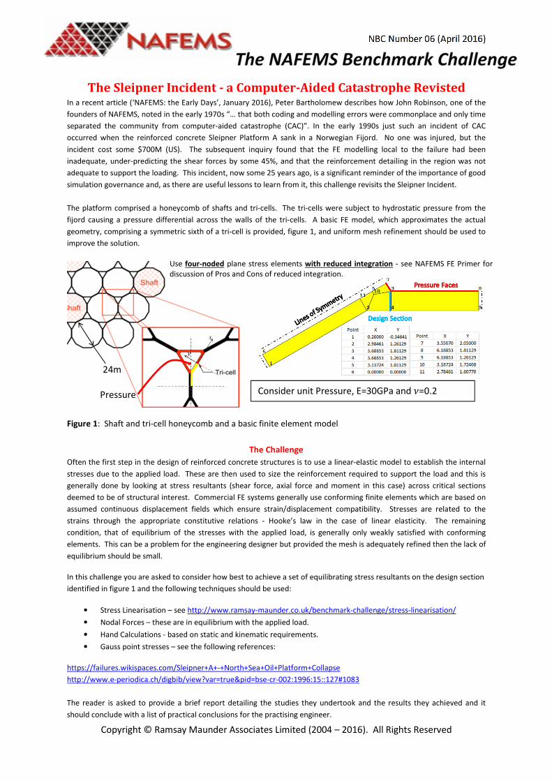
The platform comprised a honeycomb of shafts and tri-cells. The tri-cells were subject to hydrostatic pressure from the

fijord causing a pressure differential across the walls of the tri-cells. A basic FE model, which approximates the actual

geometry, comprising a symmetric sixth of a tri-cell is provided, figure 1, and uniform mesh refinement should be used to

improve the solution.

Figure 1: Shaft and tri-cell honeycomb and a basic finite element model

The Challenge

Often the first step in the design of reinforced concrete structures is to use a linear-elastic model to establish the internal

stresses due to the applied load. These are then used to size the reinforcement required to support the load and this is

generally done by looking at stress resultants (shear force, axial force and moment in this case) across critical sections

deemed to be of structural interest. Commercial FE systems generally use conforming finite elements which are based on

assumed continuous displacement fields which ensure strain/displacement compatibility. Stresses are related to the

strains through the appropriate constitutive relations - Hooke’s law in the case of linear elasticity. The remaining

condition, that of equilibrium of the stresses with the applied load, is generally only weakly satisfied with conforming

elements. This can be a problem for the engineering designer but provided the mesh is adequately refined then the lack of

equilibrium should be small.

In this challenge you are asked to consider how best to achieve a set of equilibrating stress resultants on the design section

identified in figure 1 and the following techniques should be used:

• Stress Linearisation – see http://www.ramsay-maunder.co.uk/benchmark-challenge/stress-linearisation/

• Nodal Forces – these are in equilibrium with the applied load.

• Hand Calculations - based on static and kinematic requirements.

• Gauss point stresses – see the following references:

https://failures.wikispaces.com/Sleipner+A+-+North+Sea+Oil+Platform+Collapse

http://www.e-periodica.ch/digbib/view?var=true&pid=bse-cr-002:1996:15::127#1083

The reader is asked to provide a brief report detailing the studies they undertook and the results they achieved and it

should conclude with a list of practical conclusions for the practising engineer.

Consider unit Pressure, E=30GPa and �=0.2

24m

Pressure

Use four-noded plane stress elements with reduced integration - see NAFEMS FE Primer for

discussion of Pros and Cons of reduced integration.



Raison d’être for the Challenge

This challenge is an interesting one since it looks again at some of the mistakes that occurred in the

original analysis of the Sleipner Platform and thus provides a reminder, should it be needed, that

considerable care is required when dealing with finite element results.

As the engineer charged with specifying the reinforcement for the platform you are interested in

being able to establish the critical sections where the stress resultants are a maximum. If adequate

reinforcement is not placed at these sections to resist the loads, then the design will fail. The

engineer can often predict, from experience, where these sections might be and, as in the shear

resultant for the tri-cell, the magnitude of a statically determinate resultant. Statically

indeterminate stress resultants cannot be so easily determined particularly for complex structures or

components and the engineer is then required to undertake appropriate structural analysis.

If the structural analysis is performed using a standard conforming finite element (CFE) system then

the engineer will have at his disposal a set of strongly equilibrating nodal forces and a set of weakly

equilibrating finite element stress fields from which to determine the stress resultants. This

response examines the ways in which these quantities may be used to determine the stress

resultants and also how accurately they are captured. It will also look at the properties of Gauss

point stresses and expel some of the myths that exist about their properties.

Henry Petroski, in his excellent book, ‘Design Paradigms: Case Histories of Error and Judgement in

Engineering’, discusses an observation that, at least for bridges, major failures are spaced at thirty

year intervals. The reason for this is postulated as being the result of a ‘communication gap’

between one generation of engineers and the next. It is therefore appropriate that one generation

on from the Sleipner incident, practising engineers are reminded of why the failure occurred.

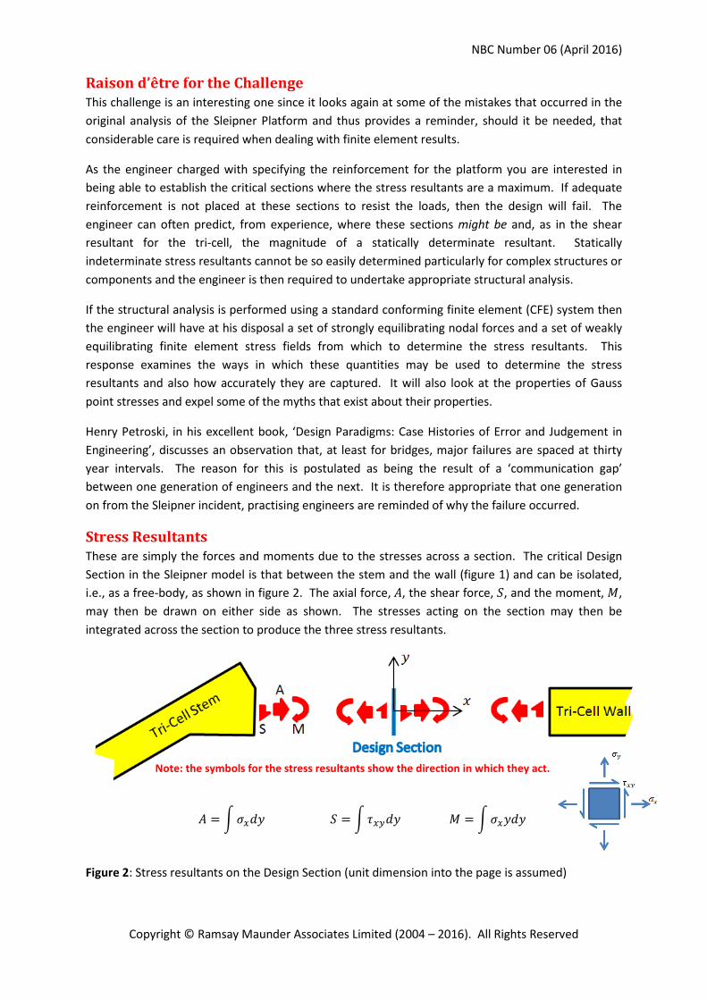
Stress Resultants

These are simply the forces and moments due to the stresses across a section. The critical Design

Section in the Sleipner model is that between the stem and the wall (figure 1) and can be isolated,

i.e., as a free-body, as shown in figure 2. The axial force,�, the shear force, �, and the moment, �,

may then be drawn on either side as shown. The stresses acting on the section may then be

integrated across the section to produce the three stress resultants.

� = �� = �� = ��

Figure 2: Stress resultants on the Design Section (unit dimension into the page is assumed)

Note: the symbols for the stress resultants show the direction in which they act.



The shear resultant is determined exactly through an assumption of symmetry and consideration of

statics. The axial force and moment resultants, however, are statically indeterminate with the exact

values depending on the relative flexibility between the stem and the wall. This can be assessed

through finite element analysis.

It is worth noting that the ideas of stress linearisation were developed in the pressure vessel industry

where the codes of practice require engineers to estimate the stress resultants at critical sections

called stress classification lines (SCL). In this challenge, we are interested in the SCL shown in figures

1 and 2.

Stress Resultants by Hand

It is always good practice, where possible, for the engineer to estimate the stress resultants by hand

calculation. The loading on the tri-cell wall is shown in figure 3 together with diagrams representing

the distributions in axial force, shear force and bending moment along the span of the beam. The

figure shows the moment resultant being equal to the fixed end moment. This would be true if the

tri-cell stem was rigid and, therefore, for the real flexible stem, the fixed end moment will provide a

conservative (upper bound) of the actual moment.

Figure 3: Hand calculation for shear and moment stress resultants

The axial stress resultant may be estimated through a consideration of the continuity of

displacements (kinematics) at the design section – see figure 4.



Figure 4: Hand calculation for axial stress resultant

The complete set of stress resultants as calculated by hand is shown in table 1. The shear resultant

is exact, the moment resultant is a conservative upper-bound value and the axial resultant is a non-

conservative lower-bound value as part of the tri-cell stem was assumed to be rigid.

Beam

Axial 1.11N

Shear 2.5N

Moment 2.083Nm

Table 1: Stress resultants from hand calculation

It should be noted here that the stress resultants calculated above are perfectly adequate for the

design of the tri-cell. It would appear, however, that the Sleipner engineers did not originally do

such a check although it is revealed in the references that the replacement for the failed platform

was designed using the sort of simple hand calculation outlined above. Acknowledging that the

engineering analysis could have stopped at this point, it is of interest to persue further the idea that

accurate stress resultants, taking account of the flexibility of the stem, should also be available from

a finite element analysis of the tri-cell.

Verification of the Finite Element System

Before launching into any finite element analysis it is wise, first, to ensure that the element type to

be used in the selected FE system is functioning correctly. Most commercial software vendors

supply benchmark problems with which they will have verified the software and which may be used

by the engineer to confirm that all is correct. Many of these benchmarks have known theoretical

solutions. In addition to checking the FE system is sound, such verification problems give the

engineer the opportunity to understand how a particular element performs, for example, in the level

of mesh refinement that might be needed to recover accurate stresses. If a benchmark problem can

be found that is similar to the actual problem considered then this will also provide an initial

understanding of how the structure works.



Given that the span/depth ratio of the tri-cell wall is relatively large, then engineer’s bending theory

may be considered valid; the influence of shear deformation will be small. If this is to be considered

as a plane elasticity problem then the stress resultants will be distributed in the form of stresses in

the usual manner for beams as shown in figure 5.

The shear stress distribution is assumed to be parabolic so that the peak value, at the centre of the section, is 1.5 times the average value.

Figure 5: Static boundary conditions for the tri-cell wall sub-model

The axial stress resultant does not change along the span of the beam whereas the shear resultant

varies linearly with span and the moment resultant quadratically as shown in figure 3. At any

position, �, along the span the shear stress varies quadratically across a section (�=constant) and the

axial stress due to the moment varies linearly. The axial and shear stresses may then be written in

terms of the stress resultants and these fields have been plotted in figure 6.

This solution for the axial and shear stress may be derived using an Airey Stress Function approach – see, for example, E.J. Hearn,

‘Mechanics of Materials’, Vol. 2, 2nd

Edition, p699, Pergamon, (1985).

Figure 6: Axial and shear stress distributions for the tri-cell wall sub-model

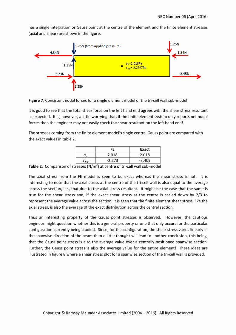
The consistent nodal forces for a single element model of the tri-cell wall are shown in figure 7. The

forces shown in blue, due to the uniformly distributed load and the shear, cancel out and thus do

not appear in the final set of consistent forces. The four-noded element with reduced integration



has a single integration or Gauss point at the centre of the element and the finite element stresses

(axial and shear) are shown in the figure.

Figure 7: Consistent nodal forces for a single element model of the tri-cell wall sub-model

It is good to see that the total shear force on the left hand end agrees with the shear stress resultant

as expected. It is, however, a little worrying that, if the finite element system only reports net nodal

forces then the engineer may not easily check the shear resultant on the left hand end!

The stresses coming from the finite element model’s single central Gauss point are compared with

the exact values in table 2.

FE Exact

� 2.018 2.018

� -2.273 -3.409

Table 2: Comparison of stresses (N/m2) at centre of tri-cell wall sub-model

The axial stress from the FE model is seen to be exact whereas the shear stress is not. It is

interesting to note that the axial stress at the centre of the tri-cell wall is also equal to the average

across the section, i.e., that due to the axial stress resultant. It might be the case that the same is

true for the shear stress and, if the exact shear stress at the centre is scaled down by 2/3 to

represent the average value across the section, it is seen that the finite element shear stress, like the

axial stress, is also the average of the exact distribution across the central section.

Thus an interesting property of the Gauss point stresses is observed. However, the cautious

engineer might question whether this is a general property or one that only occurs for the particular

configuration currently being studied. Since, for this configuration, the shear stress varies linearly in

the spanwise direction of the beam then a little thought will lead to another conclusion, this being,

that the Gauss point stress is also the average value over a centrally positioned spanwise section.

Further, the Gauss point stress is also the average value for the entire element! These ideas are

illustrated in figure 8 where a shear stress plot for a spanwise section of the tri-cell wall is provided.



Figure 8: Shear stress distribution spanwise linear, depthwise quadratic

There is another method of finding stress resultants from a finite element model and this is to

integrate the finite element stresses across the section. This method is known as stress

linearisation.

Stress Linearisation

This is a method often used in finite element analysis to obtain stress resultants on sections of

interest such as the Design Section. It performs the same integration as identified in figure 2, but on

the finite element stress and using a numerical integration scheme. The method comes from the

pressure vessel industry where the codes of practice require stress resultants to be checked at

critical sections in an axisymmetric FE model. It is important, when using this approach, that the

stresses are considered in a coordinate system normal and tangential to the section of interest. If

this is not done, then the stress resultants cannot be correctly evaluated.

In the tri-cell wall example, the direct stress parallel to a section (� ) does not contribute to the

stress resultants and the linearised value of this stress has no practical meaning. Similarly, the stress

invariants (principal stresses, von Mises stress etc.) vary in direction or indeed have no direction

along a section and thus it is difficult to see any physical meaning of linearised values of these

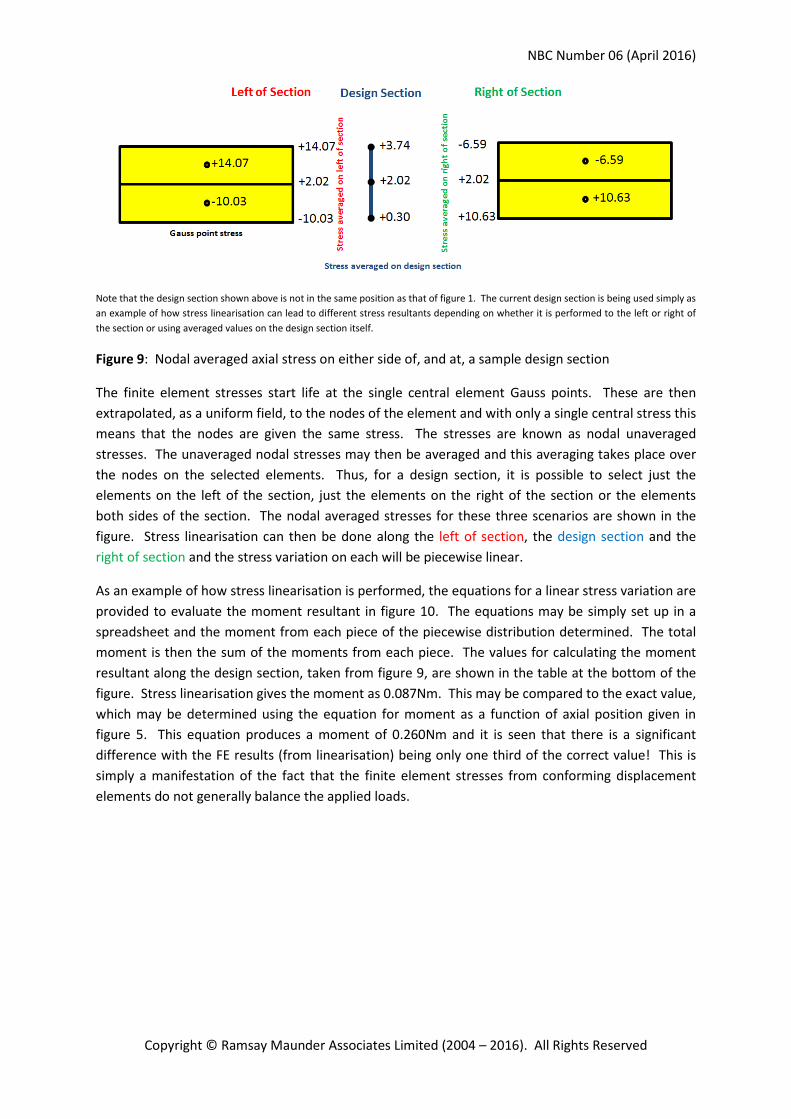
quantities. It is worth understanding how stress linearisation is performed across a section and the

axial stresses for a two element/edge mesh are shown in figure 9. Note that in this figure, the

design section refers to a section half way along the tri-cell wall and not the design section defined

in figure 1.

�� = �� ; � = 0

�� = �� ; � = 0

�� = ��

Where:

�� = � ; �� = �

; �� = � ∙ �

��

�

�

� Length Weighted Average (LWA) Shear Stress

Area Weighted Average (AWA) Shear Stress



Note that the design section shown above is not in the same position as that of figure 1. The current design section is being used simply as

an example of how stress linearisation can lead to different stress resultants depending on whether it is performed to the left or right of

the section or using averaged values on the design section itself.

Figure 9: Nodal averaged axial stress on either side of, and at, a sample design section

The finite element stresses start life at the single central element Gauss points. These are then

extrapolated, as a uniform field, to the nodes of the element and with only a single central stress this

means that the nodes are given the same stress. The stresses are known as nodal unaveraged

stresses. The unaveraged nodal stresses may then be averaged and this averaging takes place over

the nodes on the selected elements. Thus, for a design section, it is possible to select just the

elements on the left of the section, just the elements on the right of the section or the elements

both sides of the section. The nodal averaged stresses for these three scenarios are shown in the

figure. Stress linearisation can then be done along the left of section, the design section and the

right of section and the stress variation on each will be piecewise linear.

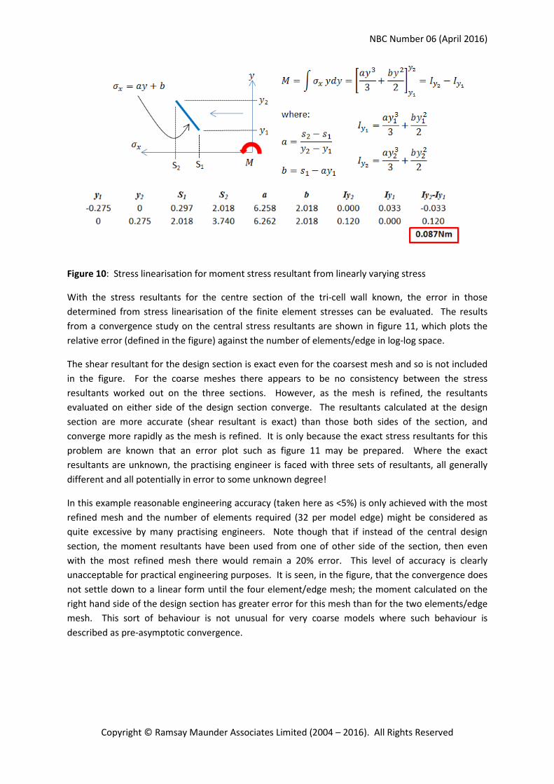
As an example of how stress linearisation is performed, the equations for a linear stress variation are

provided to evaluate the moment resultant in figure 10. The equations may be simply set up in a

spreadsheet and the moment from each piece of the piecewise distribution determined. The total

moment is then the sum of the moments from each piece. The values for calculating the moment

resultant along the design section, taken from figure 9, are shown in the table at the bottom of the

figure. Stress linearisation gives the moment as 0.087Nm. This may be compared to the exact value,

which may be determined using the equation for moment as a function of axial position given in

figure 5. This equation produces a moment of 0.260Nm and it is seen that there is a significant

difference with the FE results (from linearisation) being only one third of the correct value! This is

simply a manifestation of the fact that the finite element stresses from conforming displacement

elements do not generally balance the applied loads.



Figure 10: Stress linearisation for moment stress resultant from linearly varying stress

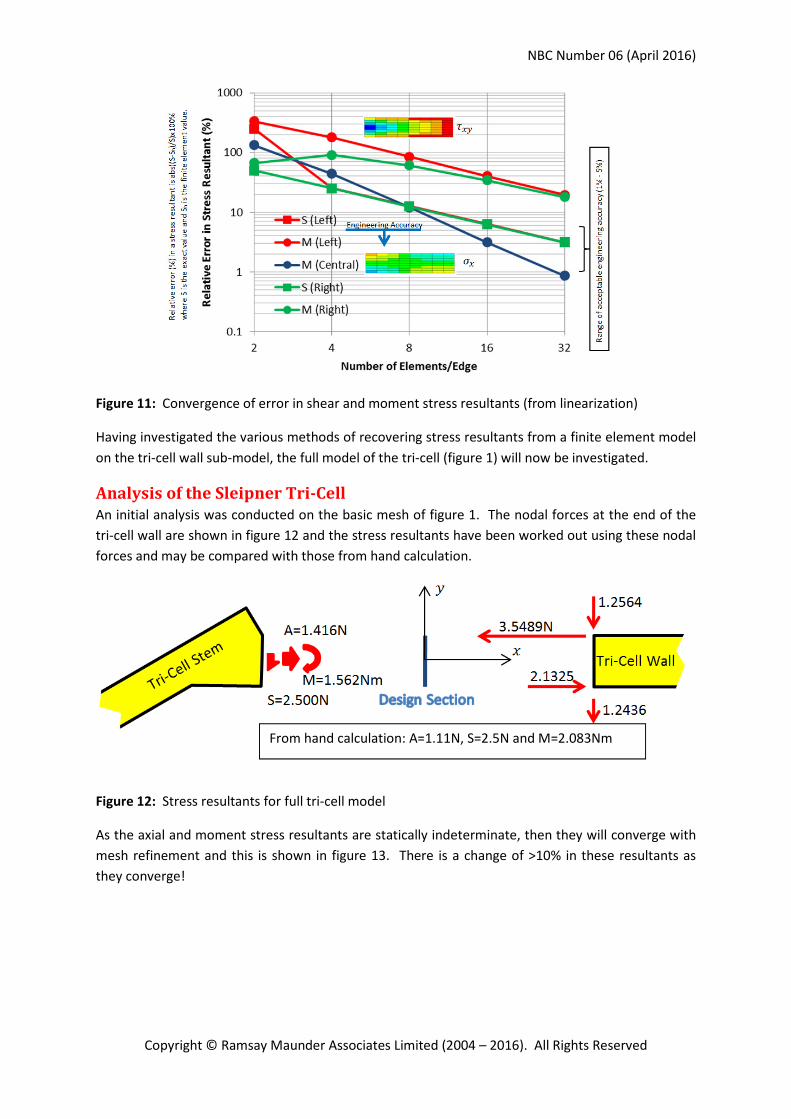
With the stress resultants for the centre section of the tri-cell wall known, the error in those

determined from stress linearisation of the finite element stresses can be evaluated. The results

from a convergence study on the central stress resultants are shown in figure 11, which plots the

relative error (defined in the figure) against the number of elements/edge in log-log space.

The shear resultant for the design section is exact even for the coarsest mesh and so is not included

in the figure. For the coarse meshes there appears to be no consistency between the stress

resultants worked out on the three sections. However, as the mesh is refined, the resultants

evaluated on either side of the design section converge. The resultants calculated at the design

section are more accurate (shear resultant is exact) than those both sides of the section, and

converge more rapidly as the mesh is refined. It is only because the exact stress resultants for this

problem are known that an error plot such as figure 11 may be prepared. Where the exact

resultants are unknown, the practising engineer is faced with three sets of resultants, all generally

different and all potentially in error to some unknown degree!

In this example reasonable engineering accuracy (taken here as <5%) is only achieved with the most

refined mesh and the number of elements required (32 per model edge) might be considered as

quite excessive by many practising engineers. Note though that if instead of the central design

section, the moment resultants have been used from one of other side of the section, then even

with the most refined mesh there would remain a 20% error. This level of accuracy is clearly

unacceptable for practical engineering purposes. It is seen, in the figure, that the convergence does

not settle down to a linear form until the four element/edge mesh; the moment calculated on the

right hand side of the design section has greater error for this mesh than for the two elements/edge

mesh. This sort of behaviour is not unusual for very coarse models where such behaviour is

described as pre-asymptotic convergence.



Figure 11: Convergence of error in shear and moment stress resultants (from linearization)

Having investigated the various methods of recovering stress resultants from a finite element model

on the tri-cell wall sub-model, the full model of the tri-cell (figure 1) will now be investigated.

Analysis of the Sleipner Tri-Cell

An initial analysis was conducted on the basic mesh of figure 1. The nodal forces at the end of the

tri-cell wall are shown in figure 12 and the stress resultants have been worked out using these nodal

forces and may be compared with those from hand calculation.

Figure 12: Stress resultants for full tri-cell model

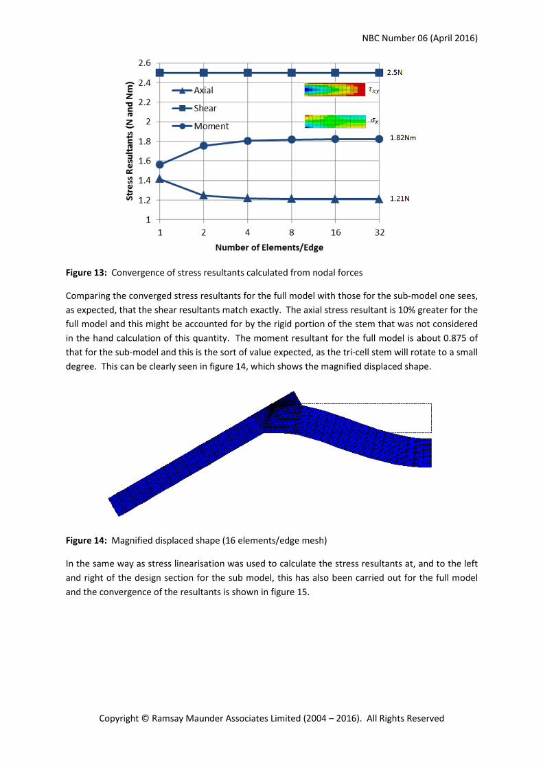
As the axial and moment stress resultants are statically indeterminate, then they will converge with

mesh refinement and this is shown in figure 13. There is a change of >10% in these resultants as

they converge!

From hand calculation: A=1.11N, S=2.5N and M=2.083Nm



Figure 13: Convergence of stress resultants calculated from nodal forces

Comparing the converged stress resultants for the full model with those for the sub-model one sees,

as expected, that the shear resultants match exactly. The axial stress resultant is 10% greater for the

full model and this might be accounted for by the rigid portion of the stem that was not considered

in the hand calculation of this quantity. The moment resultant for the full model is about 0.875 of

that for the sub-model and this is the sort of value expected, as the tri-cell stem will rotate to a small

degree. This can be clearly seen in figure 14, which shows the magnified displaced shape.

Figure 14: Magnified displaced shape (16 elements/edge mesh)

In the same way as stress linearisation was used to calculate the stress resultants at, and to the left

and right of the design section for the sub model, this has also been carried out for the full model

and the convergence of the resultants is shown in figure 15.



Figure 15: Convergence of stress resultants calculated from stress linearisation

For the coarse meshes the sign of the axial and shear resultants is incorrect on the left of the design

section and even for the most refined mesh there remains significant spread depending where the

linearisation was conducted – 0.47N in the shear which, as we know the true value to be 2.5N,

represents a difference of some 20%.

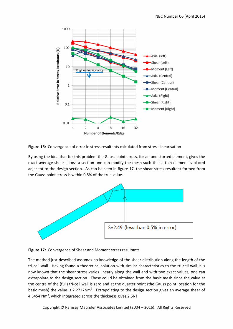
As the exact stress resultants are known for each mesh (figure 13) the error in the values from stress

linearisation may be determined and these have been plotted in figure 16. The error in the stress

resultants from linearisation is significant and for the most refined mesh only the axial and shear

resultants to the right of the design section are acceptable. If the engineer had not calculated the

exact resultants from nodal forces then he/she would have been left with having to use figure 15,

which would, to say the least, be rather unsatisfactory.

Thus, stress linearisation requires significant mesh refinement to recover accurate resultants even

for a stress field found in a beam under a uniformly distributed load – see figure 11. When the

design section goes through a point of stress singularity, then the results are polluted by the

presence of the singularity and it becomes almost impossible to make a sound engineering decision

on the data that is obtained.

Spread = 0.47N



Figure 16: Convergence of error in stress resultants calculated from stress linearisation

By using the idea that for this problem the Gauss point stress, for an undistorted element, gives the

exact average shear across a section one can modify the mesh such that a thin element is placed

adjacent to the design section. As can be seen in figure 17, the shear stress resultant formed from

the Gauss point stress is within 0.5% of the true value.

Figure 17: Convergence of Shear and Moment stress resultants

The method just described assumes no knowledge of the shear distribution along the length of the

tri-cell wall. Having found a theoretical solution with similar characteristics to the tri-cell wall it is

now known that the shear stress varies linearly along the wall and with two exact values, one can

extrapolate to the design section. These could be obtained from the basic mesh since the value at

the centre of the (full) tri-cell wall is zero and at the quarter point (the Gauss point location for the

basic mesh) the value is 2.2727Nm2. Extrapolating to the design section gives an average shear of

4.5454 Nm2, which integrated across the thickness gives 2.5N!

Engineering Accuracy



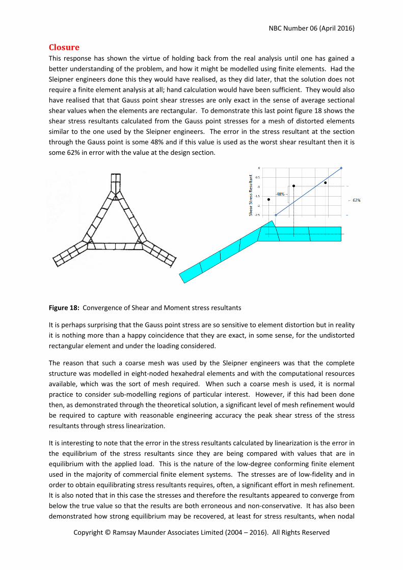
Closure

This response has shown the virtue of holding back from the real analysis until one has gained a

better understanding of the problem, and how it might be modelled using finite elements. Had the

Sleipner engineers done this they would have realised, as they did later, that the solution does not

require a finite element analysis at all; hand calculation would have been sufficient. They would also

have realised that that Gauss point shear stresses are only exact in the sense of average sectional

shear values when the elements are rectangular. To demonstrate this last point figure 18 shows the

shear stress resultants calculated from the Gauss point stresses for a mesh of distorted elements

similar to the one used by the Sleipner engineers. The error in the stress resultant at the section

through the Gauss point is some 48% and if this value is used as the worst shear resultant then it is

some 62% in error with the value at the design section.

Figure 18: Convergence of Shear and Moment stress resultants

It is perhaps surprising that the Gauss point stress are so sensitive to element distortion but in reality

it is nothing more than a happy coincidence that they are exact, in some sense, for the undistorted

rectangular element and under the loading considered.

The reason that such a coarse mesh was used by the Sleipner engineers was that the complete

structure was modelled in eight-noded hexahedral elements and with the computational resources

available, which was the sort of mesh required. When such a coarse mesh is used, it is normal

practice to consider sub-modelling regions of particular interest. However, if this had been done

then, as demonstrated through the theoretical solution, a significant level of mesh refinement would

be required to capture with reasonable engineering accuracy the peak shear stress of the stress

resultants through stress linearization.

It is interesting to note that the error in the stress resultants calculated by linearization is the error in

the equilibrium of the stress resultants since they are being compared with values that are in

equilibrium with the applied load. This is the nature of the low-degree conforming finite element

used in the majority of commercial finite element systems. The stresses are of low-fidelity and in

order to obtain equilibrating stress resultants requires, often, a significant effort in mesh refinement.

It is also noted that in this case the stresses and therefore the resultants appeared to converge from

below the true value so that the results are both erroneous and non-conservative. It has also been

demonstrated how strong equilibrium may be recovered, at least for stress resultants, when nodal



forces are used and given the poor performance of stress linearisation with low-fidelity non-

equilibrating stress fields, this approach should be favoured by the practising engineer.

In the Sleipner model, the design section had a stress singularity at one end. No standard finite

element can cope with infinite stresses and, from an engineering perspective, these are often

ignored as a manifestation of an idealised finite element model (a sharp corner in this case). If the

stress singularity is ignored then the stresses across the design section are linear and quadratic,

respectively, for the axial and shear stress. The four-noded element used in this study is not much

better than a constant stress element and, therefore, it is not surprising that it performs so poorly.

The higher-order (eight-noded) element would have performed better but, with little more than a

linear stress capability, it would still have required significant mesh refinement to achieve sensible

stress resultants. Since many practical engineering problems involve bending moments and shear

forces of the type seen in the tri-cell wall, it seems somewhat inappropriate that higher-fidelity

elements are not provided by software vendors. For example, in a displacement formulation, a cubic

(p=3) displacement field element would have recovered exactly, with a single element, the stress

field in the sub model. In the presence of the singularity in the full model, however, it would

probably have struggled and would certainly not have provided a stress field at the design section in

equilibrium with the applied loads.

Practical Conclusions

This study, based on the Sleipner failure, has provided some useful results for the practising

engineer:

1) Statically determinate stress resultants may be found by hand but statically indeterminate

ones require some form of analysis that includes the relative flexibility of the structure, e.g.,

finite element analysis.

2) Stress resultants may be determined from nodal forces if they are interpreted correctly. The

statically indeterminate resultants will converge with mesh refinement whereas statically

determinate ones are exact irrespective of the mesh chosen.

3) Gauss point stresses have certain properties that may be useful to the engineer but as these

properties do not necessarily extend to distorted elements and general stress fields the

engineer needs to be certain that they apply to his/her situation before making a potentially

rash decision to use them.

4) Stress linearisation is a valid way of determining the stress resultants across a section.

However, because CFEs provide finite element stress fields that are only weakly in

equilibrium with the applied load, then considerable mesh refinement might be needed to

obtain accurate results. If the design section runs through a point of stress singularity then

the stress field adjacent to the singularity is polluted and it is unlikely that equilibrating

stress resultants can be obtained through stress linearisation.

the sleipner incident - a computer-aided catastrophe revisted · this solution for the axial and...

Documents