the six-port technique with
TRANSCRIPT


The Six-Port Technique withMicrowave and Wireless Applications

For a listing of recent titles in theArtech House Microwave Library,
turn to the back of this book.

The Six-Port Technique withMicrowave and Wireless Applications
Fadhel M. GhannouchiAbbas Mohammadi

Library of Congress Cataloging-in-Publication DataA catalog record for this book is available from the U.S. Library of Congress.
British Library Cataloguing in Publication DataA catalogue record for this book is available from the British Library.
ISBN-13: 978-1-60807-033-6
Cover design by Yekaterina Ratner
© 2009 ARTECH HOUSE685 Canton StreetNorwood, MA 02062
All rights reserved. Printed and bound in the United States of America. No part of this book maybe reproduced or utilized in any form or by any means, electronic or mechanical, including pho-tocopying, recording, or by any information storage and retrieval system, without permission inwriting from the publisher. All terms mentioned in this book that are known to be trademarks orservice marks have been appropriately capitalized. Artech House cannot attest to the accuracy ofthis information. Use of a term in this book should not be regarded as affecting the validity ofany trademark or service mark.
10 9 8 7 6 5 4 3 2 1

v
Contents
Chapter 1 Introduction to the Six-Port Technique
1.1 Microwave Network Theory ........................................................................... 1 1.1.1 Power and Reflection ............................................................................... 1 1.1.2 Scattering Parameters ............................................................................... 3
1.2 Microwave Circuits Design Technologies ...................................................... 6 1.2.1 Microwave Transmission Lines ............................................................... 6 1.2.2 Microwave Passive Circuits ..................................................................... 7 1.2.3 Fabrication Technologies ....................................................................... 10
1.3 Six-Port Circuits ............................................................................................ 13 1.3.1 Microwave Network Measurements ....................................................... 13 1.3.2 Wireless Applications............................................................................. 16 1.3.3 Microwave Applications ........................................................................ 17
References ...................................................................................................... 18
Chapter 2 Six-Port Fundamentals
2.1 Analysis of Six-Port Reflectometers ............................................................... 2 2.2 Linear Model ................................................................................................. 24 2.3 Quadratic Model ............................................................................................ 26 2.4 Six- to Four-Port Reduction .......................................................................... 28 2.5 Error Box Procedure Calculation .................................................................. 31 2.6 Power Flow Measurements ........................................................................... 32 2.7 Six-Port Reflectometer with a Reference Port .............................................. 33 2.8 Measurement Accuracy Estimation ............................................................... 34
References ..................................................................................................... 36
Chapter 3 The Design of Six Port Junctions
3.1 Design Consideration for Six-Port Junctions ................................................ 39 3.2 Waveguide Six-Port Junctions ...................................................................... 41 3.3 Frequency Compensated Optimal Six-Port Junctions ................................... 43 3.4 Frequency Compensated Quasi-Optimal Six-Port Junctions ........................ 49 3.5 A Six-Port Junction Based on a Symmetrical Five-Port Ring Junction ........ 53

vi The Six-Port Technique with Microwave and Wireless Applications
3.6 High Power Six-Port Junction in Hybrid WaveGuide/
Stripline Technology ............................................................................................. 58 3.7 Worst-Case Error Estimation ........................................................................ 59
References ..................................................................................................... 62
Chapter 4 Calibration Techniques
4.1 Calibration Method Using Seven Standards .................................................. 65 4.2 Linear Calibration Using Five Standards ...................................................... 67 4.3 Nonlinear Calibration Using Four Standards ................................................ 70 4.4 Nonlinear Calibration Using Three Standards............................................... 71 4.5 Self-Calibration Based on Active Load Synthesis ........................................ 79 4.6 Dynamic Range Extension ............................................................................ 81 4.7 Diode Linearization Technique ..................................................................... 84 4.8 Power Calibration Technique ........................................................................ 86
References ..................................................................................................... 88
Chapter 5 Six-Port Network Analyzers
5.1 General Formulation ..................................................................................... 91 5.2 Case of a Reciprocal Two-Port DUT ............................................................ 93 5.3 Case of an Arbitrary Two-Port DUT ............................................................. 94 5.4 Six-Port Based De-Embedding Technique: Theory ...................................... 96 5.5 Two-Port De-Embedding Technique ............................................................ 99 5.6 Calculation of the Error-Box Parameters .................................................... 102 5.7 Determination of S Parameters of an Arbitrary DUT .................................. 103 5.8 Tri-Six-Port Network Analyzer ................................................................... 104 5.9 N-Six-Port Network Analyzer ..................................................................... 109 5.10 A Single Six-Port N-Port Vector Network Analyzer ................................ 111 5.11 N-Port Calibration Algorithm ................................................................... 113
References ................................................................................................... 117
Chapter 6 Source Pull and Load-Pull Measurements Using the Six-Port Technique
6.1 Principles of Source-Pull/Load-Pull Measurements .................................... 119 6.2 Impedance and Power Flow Measurements with an Arbitrary Test Port
Impedance ........................................................................................................... 120 6.3 Operation of a Six-Port in Reverse Configuration ...................................... 122
6.3.1 Six-Port Reflectometer Calibration in Reverse Configuration ............. 124 6.3.2 Error Box Calculation for Reverse Six-Port Measurements ................. 127 6.3.3 Discussion ............................................................................................ 128
6.4 Source-Pull Configuration Using Six-Port .................................................. 129 6.4.1 Passive Source-Pull Configuration ....................................................... 129 6.4.2 Active Source-Pull Configuration ........................................................ 130

Introduction to the Six-Port Technique vii
6.5 Load-Pull Configuration Using Six-Port ..................................................... 131 6.5.1 Passive Load-Pull Configuration .......................................................... 131 6.5.2 Active Branch Load-Pull Configuration .............................................. 133 6.5.3 Active Loop Load-Pull Configuration .................................................. 134
6.6 Source-Pull/Load-Pull Configuration Using Six-Port ................................. 135 6.7 A De-Embedding Technique for On-Wafer Load-Pull Measurements ....... 136
6.7.1 Calibration and Measurement Techniques ........................................... 136 6.8 Applications of Source-Pull Measurements ................................................ 139
6.8.1 Low Noise Amplifier Characterization ................................................ 139 6.8.2 Mixer Characterization ......................................................................... 140 6.8.3 Power Amplifier Characterization ........................................................ 141
6.9 Source-Pull/Load-Pull Oscillator Measurements ........................................ 142 6.9.1 Six-Port Reflectometer with Variable Test Port Impedance ................ 143 6.9.2 Oscillator Measurements ...................................................................... 143
6.10 AM-AM/AM-PM Distortion Measurements of Microwave Transistors
Using Active Load-Pull ....................................................................................... 145 6.10.1 Principle of Operation ........................................................................ 145 6.10.2 Measurement Procedure ..................................................................... 149
6.11 Time-Domain Wave-Correlator for Power Amplifier Characterization and
Optimization ........................................................................................................ 150 6.11.1 Time-Domain Waveform Measurement ............................................. 150 6.11.2 Multiharmonic Six-Port Reflectometer .............................................. 151 6.11.3 Time-Domain Voltage and Current Measurements ............................ 154
References ................................................................................................... 157
Chapter 7 Six-Port Wireless Applications
7.1 Multiport Transceiver .................................................................................. 161 7.1.1 Multiport Modulator ............................................................................. 161 7.1.2 Multiport Demodulator......................................................................... 163
7.2 Six-Port Receiver ........................................................................................ 164 7.2.1 Five-Port Receiver ................................................................................ 168 7.2.2 Noise in Six-Port Receiver ................................................................... 171 7.2.3 Six-Port Receiver Calibration .............................................................. 176 7.2.4 Six-Port Structure Bandwidth .............................................................. 177
7.3 Six-Port in Software Radio Applications .................................................... 178 7.3.1 Five-Port Structure in Software Defined Radio Applications .............. 180
7.4 Six-Port in UWB Applications .................................................................... 182 7.4.1 Six-Port Impulse Radio Modulator ...................................................... 183 7.4.2 Six-Port Impulse Radio Demodulator .................................................. 184 7.4.3 Five-Port Receiver in UWB ................................................................. 185
7.5 Six-Port in Millimeter-Wave Radios ........................................................... 188 7.6 Comparison Between Six-Port and Conventional Receivers ...................... 192
7.6.1 RF Performance..................................................................................... 192

viii The Six-Port Technique with Microwave and Wireless Applications
7.6.2 Boundary Limitations ........................................................................... 193 7.7 Six-Port in Phased-Array Systems .............................................................. 193
References ................................................................................................... 196
Chapter 8 Six-Port Microwave Applications
8.1 Six-Port Microwave Reflectometer ............................................................. 199 8.1.1 Six-Port Reflectometer ......................................................................... 199 8.2.1 High Power Microwave Reflectometer ................................................ 202
8.2 Six-Port Wave-Correlator ........................................................................... 203 8.2.1 General Concept ................................................................................... 203 8.2.2 Calibration System ............................................................................... 204 8.2.3 Architecture of a Wave-Correlator ....................................................... 206 8.2.4 Beam Direction Finder Using a Six-Port Wave-Correlator .................. 206 8.2.5 Doppler Estimation Using a Six-Port Wave-Correlator ....................... 207
8.3 Six-Port Applications in Direction Finders ................................................. 209 8.4 Six-Port Applications in Radar.................................................................... 213
8.4.1 Six-Port Doppler Sensor ....................................................................... 213 8.4.2 Six-Port Range Sensor.......................................................................... 214 8.4.3 Radar Structure ..................................................................................... 215 8.4.4 Radar Calibration ................................................................................. 216
8.5 Antenna Measurement Using Six-Port ........................................................ 216 8.5.1 Near-Field Antenna Measurement ....................................................... 216 8.5.2 Polarization Measurement .................................................................... 218
8.6 Material Characterization Using Six-Port ................................................... 220 8.6.1 Measurement System ........................................................................... 220 8.6.2 Probe Model Analysis .......................................................................... 220 8.6.3 Probe Calibration .................................................................................. 223
8.7 Optical Measurement Using Six-Port .......................................................... 223 8.7.1 Optical Six-Port Junction Design ......................................................... 224 8.7.2 Optical Six-Port Analysis ..................................................................... 226
References ................................................................................................... 228
About the Authors ......................................................................................................... 231
Index …………………………………………………………………………………… 233

1
Chapter 1
Introduction to the Six-Port Technique
This chapter is an introductory chapter to the book and it briefly reports the basic
concepts and principles related to transmissions lines, modeling of linear
networks, defining S parameters, and some elements relevant to microwave
metrology and the design of network analyzers.
1.1 MICROWAVE NETWORK THEORY
The definition of voltages and currents for non-TEM lines is not straightforward
[1]. Moreover, there are some practical limitations when one tries to measure
voltages and currents in microwave frequencies. To solve these problems, the
incident and reflected powers and their parameters are measured in microwave
frequencies. The scattering parameters, which indeed are the parameters that can
be directly related to power measurements, are used to characterize microwave
circuits and networks.
1.1.1 Power and Reflection
Figure 1.1 shows a one-port network with input impedance Z that is connected to
the generator Vg with generator impedance Zg. Power is transmitted from the
generator to the one-port network. The current and voltage at terminal are
g
g
Vi
Z Z=
+ (1.1)
and
g
g
ZVv
Z Z=
+ (1.2)

2 The Six-Port Technique with Microwave and Wireless Applications
In order to receive the maximum available power from generator in the load, the
conjugate matched, *
gZ Z= , conditions must be realized. Let g g gZ R jX= + ;
then, under this condition, the incident current and voltage are defined as [2]
gZ
a b
V +I +
gV −
+
Figure 1.1 One-port network and extraction of incident and reflected waves using a directional
coupler.
* 2
g g
gg g
V VI
RZ Z+ = =
+ (1.3)
and
* *
* 2
g g g g
gg g
Z V Z VV
RZ Z+ = =
+ (1.4)
The relationship between incident voltage and incident current is given by
*
gV Z I+ += (1.5)
The maximum available power is
2
*Re( )4
g
Ag
VP VI
R= =
(1.6)
where current and voltage are RMS values. As may be seen from (1.4) and (1.5),
incident voltage and incident current are independent of the impedance of the one-
port network. The terminal voltage and current according to Figure 1.1 are
obtained as
V V V+ −= + (1.7a)

Introduction to the Six-Port Technique 3
I I I+ −= − (1.7b)
From (1.6), the incident power is defined as the maximum available power from a
given generator as
2
*Re ( )4
g
incg
VP V I
R+ + = =
(1.8)
By using (1.4), the incident power (1.8) can be written as
2
2*
g
inc
g
V RP
Z
+
= (1.9)
The magnitude of the normalized incident wave, a, and reflected wave, b, are
defined as the square root of the incident and reflected powers as
*
g
inc gg
V Ra P I R
Z
+
+= = = (1.10a)
*
g
r gg
V Rb P I R
Z
−
−= = = (1.10b)
The dimensions of a and b are the square root of power. They are directly related
to power flow. The ratio of the normalized reflection wave to normalized incident
wave is called reflection coefficient
b
aΓ = (1.11)
1.1.2 Scattering Parameters
The normalized incident and reflected waves are related by scattering matrix. The
scattering matrix characterizes a microwave network at a given frequency and
operating conditions. Let the characteristics impedance of the transmission lines
in Figure 1.2 be equal to Z0; then the scattering matrix of a two-port network can
be represented as
1 11 12 1
2 21 22 2
b s s a
b s s a
=
(1.12)

4 The Six-Port Technique with Microwave and Wireless Applications
0Z
1a
TWO- PORT
NETWORK
1b 2b 2a
0TLZ Z= 0TLZ Z=Input Output
Figure 1.2 Two-port network and extraction of incident and reflected waves using directional coupler.
where 2
11 1 1 0/
as b a
== is the input reflection coefficient while the output is
terminated with Z0,
221 2 1 0
/a
s b a=
= is the forward transmission coefficient between Z0 terminations,
112 1 2 0
/a
s b a=
= is the reverse transmission coefficient between Z0 terminations,
and 1
22 2 2 0/
as b a
== is the output reflection coefficient while the input is
terminated with Z0.
If we have a lossless passive two-port, the power applied to the input port is
either reflected or transmitted. Accordingly,
2 2
11 21 1s s+ = (1.13)
The advantage of scattering parameters is that they can be evaluated by attaching
direction couplers to all of the network ports. The directional couplers separate
incident and reflected power waves directly, simplifying the measurement
procedure. The fact to remember is that the conditions required for determining
the individual s-parameter value need properly terminated transmission lines at the
various ports [3].
The scattering matrix may be expanded to define any N-port network, where N is
any positive integers. The characteristic impedance of the different port can be the
same. This is the case in the many practical applications. However, the scattering
matrix can be generalized to include the different characteristic impedances in
various ports [1]. An N-port network is shown in Figure 1.3, where an is the
incident wave in port n and bn is the reflected wave in port n.

Introduction to the Six-Port Technique 5
1a1b 01Z
0NZNb Na
nanb 0nZ
1Port −
Port n−
Port N−
Figure 1.3 An arbitrary N-port microwave network.
The scattering matrix, or [S] matrix, is defined in relation to these incident and
reflected waves as
1 11 12 1 1
2 21 2
1
N
N N NN N
b s s s a
b s a
b s s a
=
⋯
⋮
⋮ ⋮
⋯
(1.14)
A specific element of [S] matrix is defined as
,
0/
ki j i j a for k j
s b a= ≠
= (1.15)
A vector network analyzer is mostly used to measure the scattering parameters. A
vector network analyzer is basically a four-channel microwave receiver that
processes the amplitude and phase of the transmitted and reflected waves from a
microwave network.
A vector network analyzer generally includes three sections: RF source and test
set, IF processing, and digital processing. To measure the scattering parameters of
a DUT, RF source sweep over a specific bandwidth, the four-port reflectometer
samples the incident, reflected and transmitted RF waves, and a switch allows the
network to be driven from either ports of DUT.
6 The Six-Port Technique with Microwave and Wireless Applications
1.2 MICROWAVE CIRCUITS DESIGN TECHNOLOGIES
1.2.1 Microwave Transmission Lines
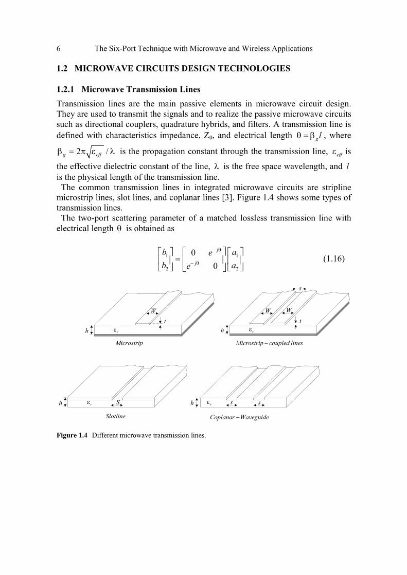
Transmission lines are the main passive elements in microwave circuit design.
They are used to transmit the signals and to realize the passive microwave circuits
such as directional couplers, quadrature hybrids, and filters. A transmission line is
defined with characteristics impedance, Z0, and electrical length g lθ = β , where
2 /g effβ = π ε λ is the propagation constant through the transmission line, εeff is
the effective dielectric constant of the line, λ is the free space wavelength, and l
is the physical length of the transmission line.
The common transmission lines in integrated microwave circuits are stripline
microstrip lines, slot lines, and coplanar lines [3]. Figure 1.4 shows some types of
transmission lines.
The two-port scattering parameter of a matched lossless transmission line with
electrical length θ is obtained as
1 1
2 2
0
0
j
j
b ae
b ae
− θ
− θ
=
(1.16)
W
t
h rε
Microstrip
W
t
h rε
W
s
Microstrip coupled lines−
Sh rε
Coplanar Waveguide−Slotline
sh rε s
Figure 1.4 Different microwave transmission lines.

Introduction to the Six-Port Technique 7
gZ
l
gV LZ0Z lθ = β
inZ
Figure 1.5 A terminated transmission line.
In practice, a transmission line is terminated to a load. A terminated transmission
line is shown in Figure 1.5. Let us assume that the load impedance is LZ , the
physical length and the characteristic impedance of the transmission line l, 0Z ,
respectively. By use of the classic transmission lines theory, it can be shown that
the input impedance of a lossless terminated transmission line is obtained as [1]
0
0
0
tan( )
tan( )
Lin
L
Z jZ lZ Z
Z jZ l
+ β=
+ β (1.17)
1.2.2 Microwave Passive Circuits
A microwave subsytem includes transmission lines, passive circuits, and active
devices. The passive circuits are the key sections in microwave signal processing.
These circuits are usually realized using transmission lines and lump elements. In
this section, some microwave passive circuits, which are commonly used in
microwave signal processing and multiport architectures, are explained.
Wilkinson Power Divider A Wilkinson power divider is shown in Figure 1.6. This
divider is used to in-phase split the power. Although this circuit can be used for
arbitary power division, the equal split power divider (3 dB) is more common.
This divider is often made in microstrip or stripline. The scattering parameter of
an ideal Wilkinson power divider can be shown as
[ ]0 / 2 / 2
/ 2 0 0
/ 2 0 0
j j
S j
j
− −
= − −
(1.18)

8 The Six-Port Technique with Microwave and Wireless Applications
Input
/ 4λ
02Z
02Z
02Z
0Z
0Z
0Z
Wilkinson Power Divider
Directional
Coupler
Isolated
Through
Coupled
Directional Coupler
0 / 2Z
0 / 2Z
0Z0Z
0Z 0Z
0Z0Z
/ 4λ02Z
0Z
0Z
0Z
0Z
1
2
3
4
∑
∆
/ 4λ
/ 4λ
/ 4λ
3 / 4λ
Figure 1.6 Some microwave passive circuits.
Directional Coupler A directional coupler is a four-port circuit matched at all
ports. The scattering matrix of a symmetrical direction coupler is as
[ ]
0 0
0 0
0 0
0 0
j
jS
j
j
α β α β = β α
β α
(1.19)
where the amplitudes α and β are related as
2 2 1α + β =
(1.20)

Introduction to the Six-Port Technique 9
According to (1.18), power supplied to port 1 is coupled to port 3 (the coupled
port) with the coupling factor 2 2
13s = β , while the reminder of the input power is
delivered to port 2 (the through port) with the coefficient 2 2 2
12 1s = α = − β . In an
ideal directional coupler, no power is delivered to port 4 (the isolated port). The
following relations are generally used to characterize a directional coupler [1]:
1
3
10log 20log dBP
Coupling CP
= = = − β (1.21a)
3
2
4 14
10log 20log dBP
Directivity DP s
β= = = (1.21b)
21
14
4
10log 20log dBP
Isolation I sP
= = = −
(1.21c)
Quadrature Hybrid Couplers Hybrid couplers are special cases of direction
couplers, where the coupling factor is 3 dB. A hybrid coupler is shown in Figure
1.6. The qudrature hybrid has a 90 degree phase shift between ports 2 and 3 when
fed at port 1. The scattering matrix for a quadrature coupler is as
[ ]
0 1 0
1 0 01
0 0 12
0 1 0
j
jS
j
j
=
(1.22)
Rat-Race Couplers A rat-race coupler, shown in Figure 1.6, has a 180 degree
phase difference between port 2 and 3 when fed at port 4. The scattering matrix of
a rat-race coupler is
[ ]
0 1 1 0
1 0 0 11
1 0 0 12
0 1 1 0
S
− =
−
(1.23)
The microwave circuits commonly use the passive circuits including transmission
lines, couplers, lumped elements, and resonators. Table 1.1 shows the different
uses of microwave passive technologies.

10 The Six-Port Technique with Microwave and Wireless Applications
Table 1.1 Passive Circuit Technologies
Application
Versus
Devices
Matching
Circuits
Signal
Filtering
Signal/
Dividing/
Combining
Device
Biasing
Impedance
Transformer
Phase
Transformer
Transmission Lines
High High High High High High
Coupled Lines Low Moderate High Low Low High
Lumped Elements
Yes
(Low
freq.)
Moderate
(Low
freq.)
Low High Low No
Hybrid Couplers
No Low High No Low Yes
Discontinuities High High Low Yes Low No
Resonators Moderate High No No No No
1.2.3 Fabrication Technologies
Microwave and RF passive and active circuits are realized by use of transmission
lines, microwave passive circuits, and solid state devices. Moreover, the
wireless and microwave systems demand smaller size, lighter weight, and lower
cost. Microwave solid state devices are an integral part of technology
advancement using different fabrication technologies. The modern microwave
circuits are usually fabricated by the use of microwave integrated circuits (MIC)
monolithic hybrid microwave integrated circuits (MHMIC), and monolithic
microwave integrated circuits (MMIC)
1.2.3.1 Microwave Solid State Devices
The microwave solid state devices are generally categorized into two main
groups: microwave diodes and microwave transistors. The microwave diodes have
different applications in microwave systems including detecting, mixing,
switching, and oscillating. A Schottky diode is usually used for mixing and
detection applications, while for attenuation and switching applications, a PIN
diode usually is recommended.
In varactor diode, the nonlinear behavior of the PN junction capacitance is used.
Varactor diodes are commonly used for resonance phase shifting applications. A
Gunn diode is a negative resistance device and its power properties depend on the
behavior of bulk semiconductor rather than junction. The main application of this
device is in designing oscillators.
On the other hand, the microwave transistors are the key devices to realize
microwave active circuits. The various types of transistors that find their use in
microwave applications are bipolar junction transistors (BJT) field effect
transistors (FET), metal-semiconductor field effect transistors (MESFET),
Introduction to the Six-Port Technique 11
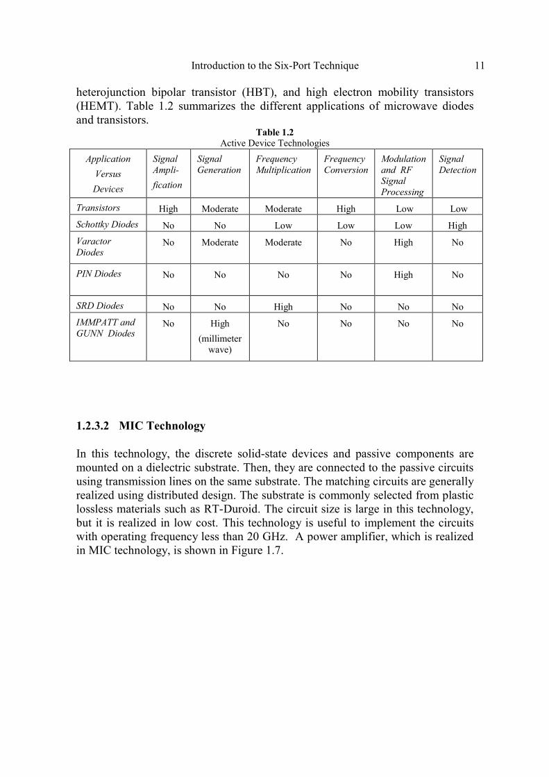
heterojunction bipolar transistor (HBT), and high electron mobility transistors
(HEMT). Table 1.2 summarizes the different applications of microwave diodes
and transistors. Table 1.2
Active Device Technologies
Application
Versus
Devices
Signal Ampli-
fication
Signal Generation
Frequency Multiplication
Frequency Conversion
Modulation and RF Signal Processing
Signal Detection
Transistors High Moderate Moderate High Low Low
Schottky Diodes No No Low Low Low High
Varactor Diodes
No Moderate
Moderate No High
No
PIN Diodes No No No No High
No
SRD Diodes No No High No No No
IMMPATT and GUNN Diodes
No High
(millimeterwave)
No No No No
1.2.3.2 MIC Technology
In this technology, the discrete solid-state devices and passive components are
mounted on a dielectric substrate. Then, they are connected to the passive circuits
using transmission lines on the same substrate. The matching circuits are generally
realized using distributed design. The substrate is commonly selected from plastic
lossless materials such as RT-Duroid. The circuit size is large in this technology,
but it is realized in low cost. This technology is useful to implement the circuits
with operating frequency less than 20 GHz. A power amplifier, which is realized
in MIC technology, is shown in Figure 1.7.

12 The Six-Port Technique with Microwave and Wireless Applications
Figure 1.7 A power amplifier in MIC technology.
1.2.3.3 MHMIC Technology
In MHMIC technology, the substrate is usually alumina due to its high
permittivity (about 10) and very low loss. The chip devices and circuits are used
in this technology and the matching is realized using both distributed and lumped
designs. The circuit size in this technology is small and its cost is moderate. This
technology can be used to realize microwave circuits up to 50 GHz. A typical
circuit fabricated using MHMIC technology is shown in Figure 1.8.
Figure 1.8 A six-port junction with integrated power detectors in MHMIC technology.

Introduction to the Six-Port Technique 13
Figure 1.9 A Ku band I-Q vector modulator using CPW transmission line in MMIC.
1.2.3.4 MMIC Technology
In MMIC, by use of silicon, GaAs, or SiGe fabrication processes, the active
devices are fabricated on substrate and passive devices are printed on substrate.
The matching circuits are on-chip lumped or distributed. The circuit size is very
small and the cost for high volume is low. The power handling in this technology
is medium. The technology can efficiently be used in microwave and millimeter-
wave circuits up to 100 GHz. A six-port junction designed with an MMIC
technology and using coplanar waveguide transmission line is shown in Figure
1.9.
1.3 SIX-PORT CIRCUITS
1.3.1 Microwave Network Measurements
The microwave and wireless technology are founded based on microwave
network measurements. A microwave network analyzer consists of a computer
controlled automated measurement setup including a synthesizer source, a test-set,
a receiver, and processing and display units. The network analyzer contains the
required directional couplers and switches to measure one- or two-port networks.
The main block of a vector network analyzer is shown in Figure 1.10. The full [S]
parameters matrix measurement of a two-port requires two different setups [4].
The basic network analyzer has a synthesized RF source with Z0 output impedance
(characteristic and line impedance) and three RF input ports.

14 The Six-Port Technique with Microwave and Wireless Applications
R
Network
Analyzer
Output Data−Phase Lock in Loop− −
AB
DUT
Figure 1.10 Block diagram of a vector network analyzer.
From these three ports, port R (reference) is used to measure the incident voltage
of the applied RF signal, and the other two measure incident and reflected waves.
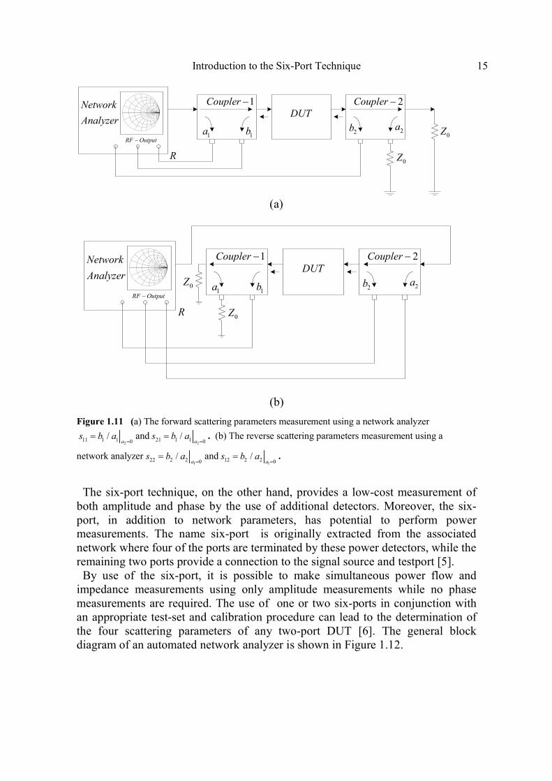
The reflection in port 1 , s11, and the forward scattering parameters of a two-port,
s21, are determined by using the setup of Figure 1.11(a).The direction couplers
have Z0 characteristic impedances. Accordingly, they present Z0 terminations to
the two-port that includes the device under test (DUT). The reflection in port 1 is
computed from the complex ratio of 1 1/b a . The forward transmission from the
source to the load is computed using 2 1/b a .
The reflection in port 2, s22, and the reverse transmission parameter, s12, are
measured using Figure 1.11(b). In this setup the signal is applied to the output port
while terminating the input port of the DUT with Z0 through coupler 1. The
reflection of the output port is obtained by the ratio of 2 2/b a . The reverse
transmission is computed from 1 2/b a . The computerized storage and use of
calibration data permit one to realize accurate and de-embedded measurements up
to the device access ports.
A key element in the implementation of vector network analyzer (VNA) is a
detection system that provides both amplitude and phase responses. The detection
section is conventionally realized using heterodyne architecture involving multiple
frequency conversion and the associated local oscillators. These components make
the measurement system relatively complex and costly. However, a heterodyne
VNA generally provides a better dynamic range compared to a homodyne VNA
six-port network analyzer, which is described in Chapter 5. The source-pull and
load-pull measurement techniques using six-port VNA are discussed in Chapter 6.
Introduction to the Six-Port Technique 15
0Z1a 1b
R
DUT1Coupler −Network
Analyzer
RF Output−
2Coupler −
2b 2a
0Z
(a)
1a 1b
R
DUT1Coupler −Network
Analyzer
RF Output−
2Coupler −
2b 2a0Z
0Z
(b)
Figure 1.11 (a) The forward scattering parameters measurement using a network analyzer
211 1 1 0
/a
s b a=
= and2
21 1 1 0/
as b a
== . (b) The reverse scattering parameters measurement using a
network analyzer1
22 2 2 0/
as b a
== and
112 2 2 0
/a
s b a=
= .
The six-port technique, on the other hand, provides a low-cost measurement of
both amplitude and phase by the use of additional detectors. Moreover, the six-
port, in addition to network parameters, has potential to perform power
measurements. The name six-port is originally extracted from the associated
network where four of the ports are terminated by these power detectors, while the
remaining two ports provide a connection to the signal source and testport [5].
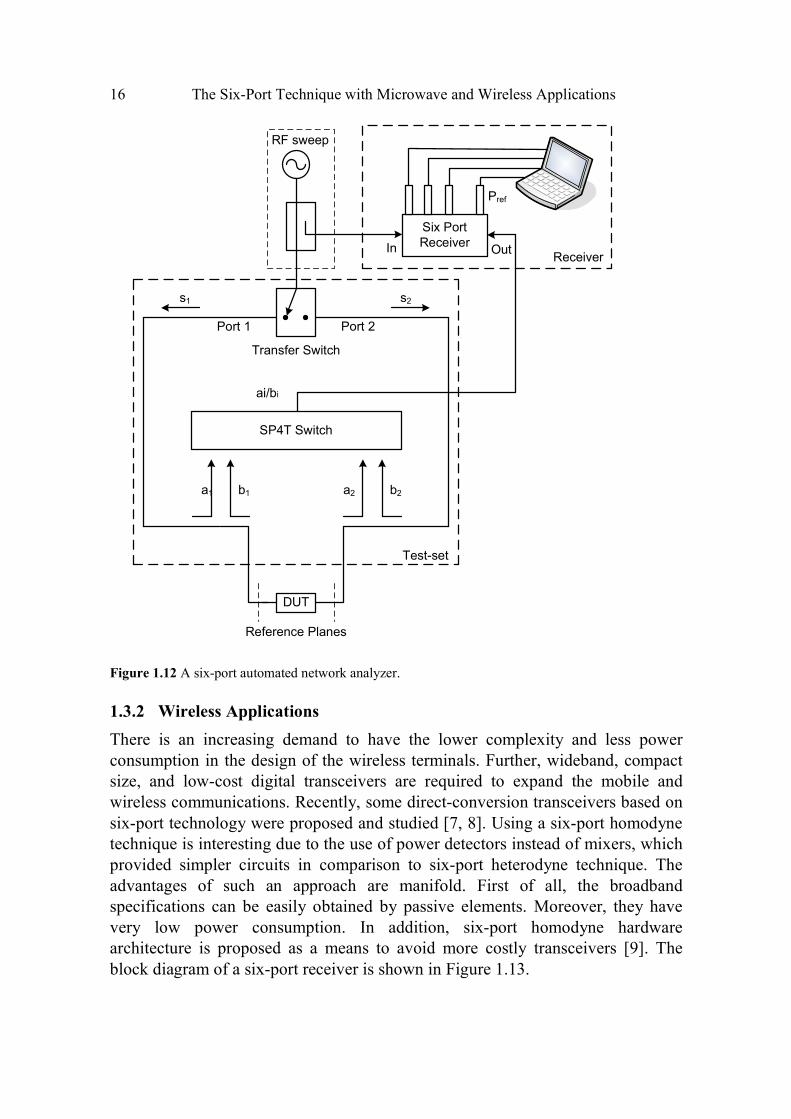
By use of the six-port, it is possible to make simultaneous power flow and
impedance measurements using only amplitude measurements while no phase
measurements are required. The use of one or two six-ports in conjunction with
an appropriate test-set and calibration procedure can lead to the determination of
the four scattering parameters of any two-port DUT [6]. The general block
diagram of an automated network analyzer is shown in Figure 1.12.
16 The Six-Port Technique with Microwave and Wireless Applications
OutIn
Six Port
Receiver
Pref
SP4T Switch
DUT
a2 b2a1 b1
s1 s2
Transfer Switch
Port 2Port 1
Reference Planes
Test-set
ai/bi
Receiver
RF sweep
Figure 1.12 A six-port automated network analyzer.
1.3.2 Wireless Applications
There is an increasing demand to have the lower complexity and less power
consumption in the design of the wireless terminals. Further, wideband, compact
size, and low-cost digital transceivers are required to expand the mobile and
wireless communications. Recently, some direct-conversion transceivers based on
six-port technology were proposed and studied [7, 8]. Using a six-port homodyne
technique is interesting due to the use of power detectors instead of mixers, which
provided simpler circuits in comparison to six-port heterodyne technique. The
advantages of such an approach are manifold. First of all, the broadband
specifications can be easily obtained by passive elements. Moreover, they have
very low power consumption. In addition, six-port homodyne hardware
architecture is proposed as a means to avoid more costly transceivers [9]. The
block diagram of a six-port receiver is shown in Figure 1.13.

Introduction to the Six-Port Technique 17
Figure 1.13 Direct conversion receiver based on six-port.
The main advantage of the six-port is the extremely large frequency bandwidth
of the RF circuit. The other advantage of the six-port system is similar to that of
the zero-intermediate frequency (IF) mixer based receiver (i.e., one local oscillator
and no image rejection filter). The six-port transceiver architectures introduce
various applications including software defined radio (SDR), ultra wideband
system (UWB), and millimeter-wave [10–12].
Six-port has attracted much attention as a low-cost transceiver in new wireless
standards. Recently, a six-port transceiver was implemented using CMOS
technology in 60 GHz [13]. The target is to provide a very low-cost, miniaturized,
and low DC power consumption transceiver for IEEE 802.15 applications. It is
shown that the total DC power consumption of the transceiver is less than 100
mW. The wireless applications of six-port technology are extensively discussed
in Chapter 7.
1.3.3 Microwave Applications
The six-port technique has great potential in microwave applications where
measuring the phase and amplitude of a microwave signal is required. A common
application is the reflectometer where the reflection coefficient of device under
test (DUT) is measured [5]. The directional finding of the received waveform is
the other application where a six-port may be used as a wave correlated [14].
The six-port application in radar is shown in Figure 1.14. This technology has
attracted attention to realize low-cost and high performance radar, especially in
the automobile industry [15]. Moreover, antenna measurement, including the
near-field and polarization measurement, can be achieved using six-port
technology.

18 The Six-Port Technique with Microwave and Wireless Applications
1a 2a
f f+ ∆
f
d
Figure 1.14 Block diagram of a six-port radar system.
The material characterization, especially in high power applications, is a very
interesting use of this technology [16]. Moreover, there are recently some
applications to use the six-port architecture in optical systems [17]. The
microwave applications of six-port systems are presented in Chapter 8.
References
[1] Pozar, D. M., Microwave Engineering, Third Edition, New York: John Wiley & Sons, 2005.
[2] Vendelin, G. D., A. M. Pavio, and U. L. Rohde, Microwave Circuit Design Using Linear and Nonlinear Techniques, Second Edition, New York: Wiley-Interscience, 2005.
[3] Maloratsky, L. G., Passive RF & Microwave Integrated Circuits, New York: Elsevier, 2004.
[4] Besser, L., and R. Gilmore, Practical RF Circuit Design for Modern Wireless Systems, Volume
1, Norwood, MA: Artech House, 2003.
[5] Engen, G. F., Microwave Circuit Theory and Foundation of Microwave Metrology, IEE
Electrical Measurement Series 9, London: Peter Peregrinus Ltd., 1992.
[6] Ghannouchi, F. M., Y. Xu, and R. G. Bosisio, “A One-Step Connection Method for the Measurement of N-Port Microwave Networks Using Six Port Techniques,” IEE Proceedings Part-H. Microwave, Antenna & Propagation, Vol. 141, No. 4, pp. 285–289, August 1994.
[7] Bosisio, R.G., Y. Y. Zhao, X. Y. Xu, S. Abielmona, E. Moldovan, Y. S. Xu, M. Bozzi, S. O. Tatu, J. F. Frigon, C. Caloz, and K. Wu, “New-Wave Radio,” IEEE Microwave Magazine, pp.
89–100, February 2008.
[8] Luo, B., and M. Y. W. Chia, “Performance Analysis of Serial and Parallel Six-Port Modulators,” IEEE Trans. Microwave Theory & Tech., Vol. 56, No. 9, September 2008.
[9] Boulejfen, N., F. M. Ghannouchi, and A. B. Kouki, “A Homodyne Multiport Network Analyzer
for S-Parameter Measurements of Microwave N-Port Circuits/Systems,” Microwave & Optical Technology Letters, Vol. 24, No.1, pp. 63–67, January 2000.
[10] Mohajer, M., A. Mohammadi, and A. Abdipour, “Direct Conversion Receivers Using Multi-Port
Structures for Software Defined Radio Systems,” IET Microwaves, Antennas & Propagation, Vol. 1, No. 2, pp. 363–372, April 2007.
[11] Zhao, Y., J. F. Frigon, K.Wu, and R. G. Bosisio, “Multi(Six)-Port Impulse Radio for Ultra-
Wideband,” IEEE Trans. Microwave Theory & Tech., Vol. 54, No. 4, pp. 1707–712, June 2006.

Introduction to the Six-Port Technique 19
[12] Mirzavand, R., A. Mohammadi, and A. Abdipour, “Low-Cost Implementation of Broadband
Microwave Receivers in Ka Band Using Multi-Port Structures,” IET Microwaves, Antennas & Propagation, Vol. 3, No. 3, pp. 483–491, 2009.
[13] Wang, H., K. Lin, Z. Tsai, L. Lu, H. Lu, C. Wang, J. Tsai, T. Huang, and Y. Lin, “MMICs in the
Millimeter-Wave Regime,” IEEE Microwave Magazine, pp. 99–117, February 2009.
[14] Yakabe, T., F. Xiao, K. Iwamoto, F. M. Ghannouchi, K. Fujii, and H. Yabe, “Six-Port Based
Wave-Correlator with Application to Beam Direction Finding,” IEEE Trans. on Instrumentation and Measurements, Vol. 50, No. 2, pp. 377–380, April 2001.
[15] Miguelez, C. G., B. Huyart, E. Bergeault, and L. P. Jallet, “A New Automobile Radar Based on
the Six-Port Phase/Frequency Discriminator,” IEEE Trans. Vehicular Tech., Vol. 49, No. 4, pp.
1416–1423, July 2000.
[16] Caron, M., A. Akyel, and F. M. Ghannouchi, “A Versatile Easy to Do Six-Port Based High Power
Reflectometer,” Journal of Microwave Power and Electromagnetic Energy, Vol. 30, No. 4, pp.
23–239, 1995.
[17] Fernandez, I. M., J. G. Wanguemert-Pérez, A. O. Monux, R. G. Bosisio, and K. Wu, “Planar
Lightwave Circuit Six-Port Technique for Optical Measurements and Characterizations,” Journal of Lightwave Technology, Vol. 23, No. 6, pp. 2148–2157, June 2005.


21
Chapter 2
Six-Port Fundamentals
The basic work related to the six-port technique was carried out in the 1970s
primarily by Engen and Hoer [1–4]. Since that time, many researchers have been
involved in six-port measurement techniques from the theoretical side as well as
the experimental side [5–14]. The main advantage of this technique is its
capability to make impedance measurement and network analysis using only
scalar measurements such as power or voltage measurement. No phase
measurements are required; hence, no frequency downconversion is needed for
the measurements. This simplifies a lot the hardware requirements and reduces
the cost of the equipment. In addition, the six-port technique can be used to make
multiport measurements and can also be used for power measurements. In this
chapter, the fundamentals of the six-port technique and the analysis and the
modeling of the six-port reflectometer are presented. Some practical
considerations are also discussed.
2.1 ANALYSIS OF SIX-PORT REFLECTOMETERS
A six-port reflectometer is generally composed of an arbitrary, time-stationary,
linear, and passive microwave six-port junction, where four ports are fitted with
power detectors, D3, D4, D5 and D6, with port 1 connected to a microwave
source and port 2 to the device under test (DUT), as shown in Figure 2.1. ia and
ib , i = 1, 2, ..., and 6, are the incident and reflected normalized voltages at the
sixth terminal of the six-port junction. The ia and ib are related through the
scattering parameters of the six-port junction as follows:
=b Sa (2.1)

22 The Six-Port Technique with Microwave and Wireless Applications
where S is a (6×6) complex matrix, ( )1 2 6, , ,b b ... b=b and ( )1 2 6, ,...,a a a=a . Let’s
designate the reflection coefficient of the power detector Di by iΓ , such as:
Figure 2.1 A six-port reflectometer.
Γ = ii
i
a
b, i = 3, 4, 5, and 6 (2.2)
by substituting (2.2) into (2.1) and after algebraic manipulations, one can obtain
( )( )
( )( )
11 12 13 3 14 4 15 5 16 61
21 22 23 3 24 4 25 5 26 62
31 32 33 3 34 4 35 5 36 6
41 42 43 3 44 4 45 5 46 6
51 52 53 3 54 4 55 5 56 6
61 62 63 3 64 4 65 5 66 6
s s s s s s
s s s s s s
s s s 1 s s s0
s s s s 1 s s0
s s s s s 1 s0
s s s s s s 10
b
b
Γ Γ Γ Γ Γ Γ Γ Γ Γ − Γ Γ Γ
= Γ Γ − Γ Γ
Γ Γ Γ − Γ
Γ Γ Γ Γ −
1
2
3
4
5
6
a
a
b
b
b
b
(2.3)
the solution of the last matrix equation given the following:
1 11 1 12 2a m b m b= + (2.4a)
DUTZ g
D 3
a3 a5
a1
b1
a2
b2
b3
D4
a4
b4
D 5
b5
D 6
a6
b6
Six-port Junction

Six-Port Fundamentals 23
2 21 1 22 2a m b m b= + (2.4b)
and
1 1 2 2i i ib m b m b= + , i = 3, 4, 5, and 6 (2.5)
where m ij are the entries of the inverse of the (6×6) matrix introduced in (2.3).
The reflection coefficient of the DUT connected to port 2 of the six-port junction
is:
2
2
a
bΓ = (2.6)
By substituting (2.6) into (2.5) and by using (2.4), one can obtain
( )2 2
ii i i i
i
kb h b h q b
h
= Γ + = Γ −
, i = 3, 4, 5, and 6 (2.7)
where
1
21
ii
mh
m= , 22 1
2
21
ii i
m mk m
m= − , and i
i
i
kq
h= − (2.8)
The net absorbed power by the power detector Di can be calculated as follows:
( )( )
2 2
2 2 2 2 2 22
2 21
i i i i
i i i i i i i
P b a
P h q b q b
= ν −
= ν − Γ Γ − = α Γ − (2.9)
where iν is a scalar parameter that characterizes the detector and
( )2
i1i i ihα = ν − Γ , with i = 3, 4, 5, and 6 (2.10)
Equation (2.9) is a quadratic equation that relates each power reading to the
reflection coefficient Γ of the DUT. This equation constitutes the starting point of
any calibration technique. It is important to remember that this equation is
obtained for a time-stationary, passive, and linear six-port junction and no

24 The Six-Port Technique with Microwave and Wireless Applications
constraints are stated for the generator’s internal impedance and the input
impedance of the power detectors. In the case where the power detectors are perfectly matched to the output ports of
the six-port junction ( 0)iΓ = , iq point values can be directly calculated using the
S parameters of the six-port junction. In such situations, one can write:
2 21 1 22 2b s a s a= + (2.11)
and
1 1 2 2i i ib s a s a= + ; i = 3, 4, 5, and 6 (2.12)
Knowing that 2 2a b= Γ and eliminating 1a from (2.12) by using (2.11), and after
identification with (2.7), one can deduce that
2 21 22 1
21
i ii
s s s sh
s
−= and 1
22 1 2 21
ii
i i
sq
s s s s=
− (2.13)
2.2 LINEAR MODEL
Equation (2.9) can be expanded in a linear manner and grouped in matrix format
as follows:
22 2 2 * 2
3 3 3 3 3 3 33
22 2 2 * 2 22 4 4 4 4 4 4 44
2 22 2 2 * 25 5 5 5 5 5 5 5
*22 2 2 * 266 6 6 6 6 6 6
1q q qP
q q qPb
P q q qP q q q
α α −α −α α α −α −α Γ = = Γ α α −α −α Γ α α −α −α
P (2.14)
Knowing that ( )Re( ) 1 2 ∗Γ = Γ + Γ and ( )Im( ) 2j ∗Γ = Γ − Γ , one can write:
2 2
*
1 11 0 0 0
0 1 0 0
0 0 1/ 2 1/ 2Re( )
0 0 / 2 / 2Im( ) j j
Γ Γ = = Γ Γ −Γ Γ
Γ (2.15)

Six-Port Fundamentals 25
By introducing (2.15) into (2.14), one can obtain the following equation [5]:
( ) ( )( ) ( )( ) ( )( ) ( )
22 2 2 2
3 3 3 3 3 3 3
22 2 2 22 4 4 4 4 4 4 4
2 22 2 2 2
5 5 5 5 5 5 5
22 2 2 2
6 6 6 6 6 6 6
2 Re 2 Im
2 Re 2 Im
2 Re 2 Im
2 Re 2 Im
q q q
q q qb
q q q
q q q
α α − α − α α α − α − α
= = ρ α α − α − α α α − α − α
P Γ CΓ (2.16)
Where 2
2bρ = and C is a (4×4) real matrix which characterize the six-port
reflectometer.
Using (2.16), one can easily deduce that
11 1−= =ρ ρ
Γ C P XP (2.17)
The iq point values can be directly calculated using the entries of matrix C as
follows:
3 4
22
i ii
i
c jcq
c
+=
− (2.18)
We can assume that the six-port junction has qi point position values in such a
way that the determinant of C is not equal to zero. Therefore, the real and
imaginary parts of the complex reflection coefficient can be deduced as follows:
( )
4
3 2
1
4
1 2
1
Re
j jj
j jj
x P
x P
+=
+=
Γ =∑
∑
(2.19a)
( )
4
4 2
1
4
1 2
1
Im
j jj
j jj
x P
x P
+=
+=
Γ =∑
∑ (2.19b)

26 The Six-Port Technique with Microwave and Wireless Applications
where x ij are the entries of the matrix X. Equation (2.19) automatically accounts
for the fact that the measurement of the reflection coefficient of a linear DUT is
power independent. The power flow exciting the DUT is:
4
1 2
1
j jj
x P +=
ρ = ∑ (2.20)
The normalization of all entries of matrix X by x11 does not affect the above
formalism; thus, (2.17) is still valid for the calculation of Γ . In the above
formalism, eleven linearly independent real parameters are sufficient to model the
six-port reflectometer. These parameters have to be determined in advance using
an appropriate calibration technique.
2.3 QUADRATIC MODEL
It was shown for an arbitrary six-port reflectometer so that the power readings at
the four detection ports of the six-port junction are:
2 22
2i i iP q b= α Γ − , i = 3, 4, 5, and 6 (2.21)
By normalizing P4, P5 and P6 by P3, one can obtain three power independent
equations
2
2
i
3 3
i ii
P qP
P q
Γ −= = µ
Γ −, i = 4, 5, and 6 (2.22)
where
3
ii
αµ =
α (2.23)
From (2.22), it can be deduced that 11 real and independent parameters are needed
to completely model the six-port reflectometer. In addition, it can be seen that Γ
is the solution of a set of three quadratic equations.
Equation (2.22) is a circle equation that can alternatively be written in the
following format [15]:
Six-Port Fundamentals 27
22
i iR Q= Γ − i = 4, 5, and 6 (2.24)
where the center and the radius of the circles in the Γ plane are, respectively:
2
2
3 3
2
2 2
3 3
i ii
i
i i
pq
q qQ
p
q q
∗
µ−
=µ
−
(2.25a)
2
2
3 32
22
2 2
3 3
i i ii
i
i i
qp
q qR
p
q q
µ µ− +
= µ −
(2.25b)
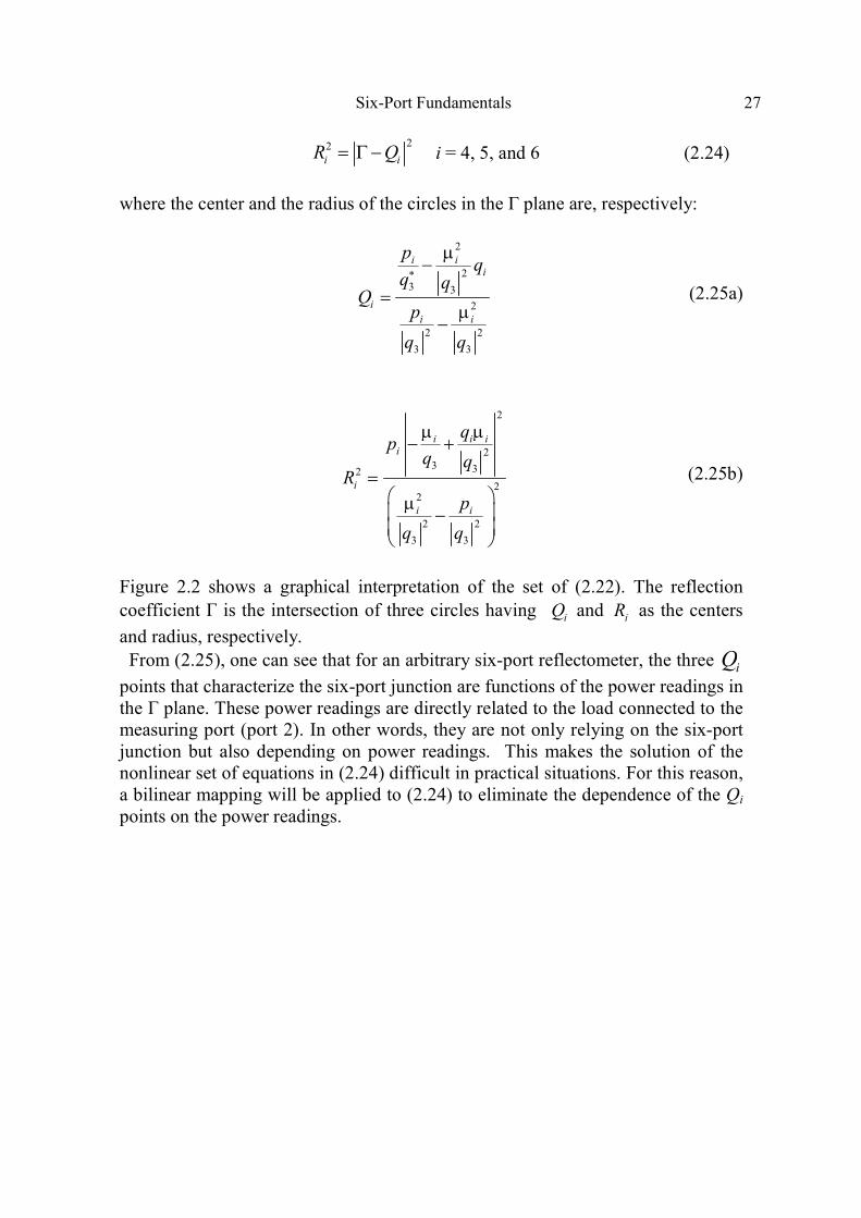
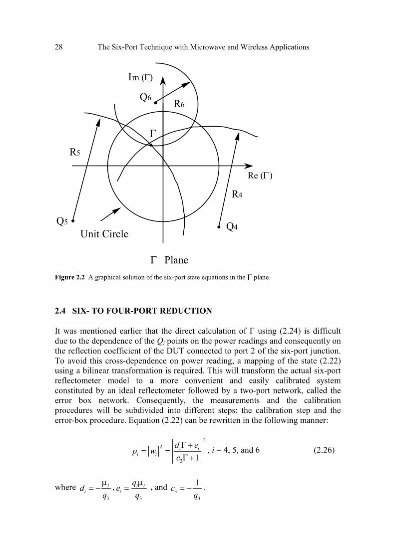
Figure 2.2 shows a graphical interpretation of the set of (2.22). The reflection
coefficient Γ is the intersection of three circles having iQ and iR as the centers
and radius, respectively.
From (2.25), one can see that for an arbitrary six-port reflectometer, the three Qi
points that characterize the six-port junction are functions of the power readings in
the Γ plane. These power readings are directly related to the load connected to the
measuring port (port 2). In other words, they are not only relying on the six-port
junction but also depending on power readings. This makes the solution of the
nonlinear set of equations in (2.24) difficult in practical situations. For this reason,
a bilinear mapping will be applied to (2.24) to eliminate the dependence of the Qi
points on the power readings.
28 The Six-Port Technique with Microwave and Wireless Applications
Q4Q5
Q6
R4
R5
R6
Unit Circle
Γ Plane
Re (Γ)
Im (Γ)
.
.
. .
Γ
Figure 2.2 A graphical solution of the six-port state equations in the Γ plane.
2.4 SIX- TO FOUR-PORT REDUCTION
It was mentioned earlier that the direct calculation of Γ using (2.24) is difficult
due to the dependence of the Qi points on the power readings and consequently on
the reflection coefficient of the DUT connected to port 2 of the six-port junction.
To avoid this cross-dependence on power reading, a mapping of the state (2.22)
using a bilinear transformation is required. This will transform the actual six-port
reflectometer model to a more convenient and easily calibrated system
constituted by an ideal reflectometer followed by a two-port network, called the
error box network. Consequently, the measurements and the calibration
procedures will be subdivided into different steps: the calibration step and the
error-box procedure. Equation (2.22) can be rewritten in the following manner:
2
2
3 1
i ii i
d ep w
c
Γ += =
Γ +, i = 4, 5, and 6 (2.26)
where
3
iid
q
µ= − ,
3
i ii
qe
q
µ= , and
3
3
1c
q= − .

Six-Port Fundamentals 29
Using (2.26), one can deduce the reflection coefficient Γ as of function wi as
follows:
5 5 6 64 4
3 4 4 3 5 5 3 6 6
e w e we w
c w d c w d c w d
− −−Γ = = =
− − − (2.27)
Using (2.27), one can derive that
3
3 3
i j j ii ii j
j j j j
d e d ee c dw w
e c d e c d
−−= +
− − (2.28)
with i = 4, 5, and 6; j = 4, 5, and 6 with i ≠ j. Using (2.28) to calculate w5 and w6 as functions of w4 and after the
substitution of their corresponding expressions (2.26), one can obtain
2
4 4p w= (2.29a)
2
5 42
5
1p w m
A= − (2.29b)
and
2
6 42
6
1p w n
A= − (2.29c)
where
4 3 4
5
5 3 5
e c dA
e c d
−=
− and 4 3 4
6
6 3 6
e c dA
e c d
−=
− (2.30a)
and
j 5 4 4 5
5 3 5
md e d e
m m ee c d
ϕ −= =
− (2.30b)
and

30 The Six-Port Technique with Microwave and Wireless Applications
j 6 4 4 6
6 3 6
nd e d e
n n ee c d
ϕ −= =
− (2.30c)
Equation (2.29) shows that the expressions of the iQ points, o, m, and n in the 4w
plane are power independent and rely only on the six-port junction. This is
opposite of the expressions of iQ points in the Γ plan; see (2.25).
Equation (2.29) is circle’s equations. The intersection of these three circles in the
4W plane provides the solution shown in Figure 2.3.
Figure 2.3 A graphical solution of the six-port state equations in the W4 plane.
Equation (2.29) can be expanded in a linear manner and grouped in a matrix
format as follows:
2
4 422
5 5 4
2 26 6 4
0 1 0 0
1
p w
A p m m m w
A p n n wn
∗ ∗
∗
= + − − − −
(2.31)
m n
W 4 Plane
ϕ m
ϕ n
| n
Re (W 4 )
I m (W 4 )
0
| m | .
.
.
.
A 5 p
5 ¦
¦ p 4
¦ 6
A 6
p W 4

Six-Port Fundamentals 31
After several matrix manipulations and one matrix inversion, one can obtain an
explicit expression to calculate w4 as function of the three normalized power
readings and the six-port calibration parameters2
5A ,2
6A , m and n . Knowing that
( )4 4 4Re( ) 1 2w w w ∗= + and ( )4 4 4
Im( ) 2w j w w ∗= − , one can deduce [1,15]:
( )( ) ( )2 22 2
4 6 6 4 5 5
4
sin sin Re
2 sin ( ) 2 sin ( )
m n
n m n m
p A p n p A p mw
n m
ϕ − + ϕ − += +
ϕ − ϕ ϕ − ϕ (2.32)
( )( ) ( )2 22 2
4 6 6 4 5 5
4
cos cos Im
2 sin ( ) 2 sin ( )
m n
n m n m
p A p n p A p mw
n m
ϕ − + ϕ − += +
ϕ − ϕ ϕ − ϕ (2.33)
The calibration parameters have to be calculated in advance using an appropriate
calibration technique. Chapter 3 is devoted to this matter.
It is important to notice that there are several choices for the definition of the
embedded reflection coefficient w4 . These choices depend on the selection of the
normalizing power reading, 3P or 4P or
5P or
6P , and on the choice of the
independent embedded reflection coefficient, w4 or w5 or w6 .
2.5 ERROR BOX PROCEDURE CALCULATION
An actual reflectometer can be modeled as an ideal reflectometer connected to an
error box network as shown in Figure 2.4. The embedded reflection coefficient,
w , is related to the de-embedded reflection coefficient, Γ , by
1
d ew
c
Γ +=
Γ + (2.34)
where ( )11 22 21 12d s s s s= − − , 11e s= , and 22c s= − and d, e, and c are three
complex parameters of the two-port network that models the transition between
the measuring plane of an ideal six-port reflectometer and the measuring plane of
an actual six-port reflectometer as shown in Figure 2.4. ijs are the scattering
parameters of the two-port error box network.

32 The Six-Port Technique with Microwave and Wireless Applications
These parameters, d, e, and c, have to be known in advance. The use of three
well-known standards, 1 2,s sΓ Γ , and 3
sΓ , allows the straightforward calculation of
the three unknown parameters by solving a set of three linear complex equations.
s s s si i i iw c d e wΓ − Γ − = and i = 1, 2, and 3 (2.35)
In practice, the short-open-load technique (SOLT) is often used in case the
measuring plane terminal of the six-port reflectometer is coaxial. The expression
of the de-embedded reflection coefficient Γ as a function of the three error box
parameters is:
e w
cw d
−Γ =
− (2.36)
Actual Reflectometer
Ideal
ReflectometerError Box
W Γ
Figure 2.4 Modeling of an actual reflectometer as an ideal reflectometer connected to an error box
network.
2.6 POWER FLOW MEASUREMENTS
The six-port reflectometer has the capability to measure the power absorbed by
any DUT without the need to use an extra power meter and without the need to
insert any coupler between the measuring port and the DUT. Using (2.9) and
(2.26), one can write:
22 2 2 22 3
3 3 3 2 3 22
3
1DUT DUTP q b c bc
α= α Γ − = Γ + (2.37)

Six-Port Fundamentals 33
and
( )2 2 2 2
2 2 21DUT DUTP b a b= − = − Γ (2.38)
By substituting the expression of 2
2b extracted from (2.37) into (2.38), one can
obtain:
( )2 2
3 3
22
3 3
1
1
DUT
DUT
DUT
c PP
c
− Γ=
α Γ + (2.39)
The only coefficient left unknown in (2.39) is2
3α . To determine this coefficient, a
power calibration has to be carried out using a precise power meter. By
connecting a power meter to the measuring port, we can calculate 2
3α as follows
( )2 2
3 32
3 2
3
1
1
PM
PM PM
c P
P c
− Γα =
Γ + (2.40)
where PMΓ and3P are, respectively, the measured reflection coefficient by the
six-port reflectometer and the measured power level at port 3 of the six-port
junction. PMP is the power measured by the standard power meter and c3 = c
(this will be proved in Chapter 4) is a complex parameter obtained during the
error-box de-embedding procedure.
2.7 SIX-PORT REFLECTOMETER WITH A REFERENCE PORT
In most practical situations, the six-port junction is designed in such a way that its
third port is isolated from the measuring port ( )32 0s ≈ and thus does not respond
significantly to the DUT. In such a case the six-port junction comprises a
reference port, 3P , which monitors the power flow exciting the DUT. In addition,
if the mismatch of the measuring port is not excessive ( )220s ≈ , the module of q3
becomes too large in comparison to Γ . Therefore, the set of (2.9) becomes:

34 The Six-Port Technique with Microwave and Wireless Applications
2 22
3 3 3 2P a q b= (2.41a)
2 22
4 4 2 4P a b q= Γ − (2.41b)
2 22
5 5 2 5P a b q= Γ − (2.41c)
2 22
6 6 2 6P a b q= Γ − (2.41d)
The division of (2.41b), (2.41c), and (2.41d) by (2.41a) leads to a similar equation
(2.24). In such a case, the iQ point expressions become independent of the power
and their expressions are the following
i iQ q= ; i = 4, 5, and 6 (2.42)
2.8 MEASUREMENT ACCURACY ESTIMATION
It was mentioned that the graphical solution of the state quadrature equations of
the six-port reflectometer is the common intersection of three circles. The centers
of these three circles are primarily determined by the six-port characteristics and
are nominally independent of the reflection coefficient of the DUT. Figure 2.3
shows that the radius of each circle is proportional to the square root of the
normalized power readings pi . In practice, due to measurement errors and
detector noises, the three circles usually do not intersect at a common point. Their
intersection will fall inside a triangle area as shown in Figure 2.5.
Assume that the four real calibration parameters, 5 6, ,A A m , and n , are known
after a suitable calibration. Generally speaking, power detectors readings 3P ,
4P ,
5P , and 6P are different from their corresponding noiseless values
3tP , 4tP ,
5tP ,
and 6tP . A maximum likelihood estimation of w via a least square procedure can
be used to find a best estimation of the reflection coefficient Γ .

Six-Port Fundamentals 35
Figure 2.5 Confidence area of six-port reflectometer measurements.
If the power detector noise is assumed to be a Gaussian distribution, it can be
shown that the maximum likelihood estimation of 3P ,
4P ,5P , and
6P is to
minimize the error function as follows:
26
3
i it
i i
P PF
=
−=
σ ∑ (2.43)
where iσ is the standard variance of the measured values iP . In order to (2.43)
for itP , it is more convenient to substitute itP as a function of 3tP .
By introducing a new parameter 3 3 3tP Pε = − and using (2.29), it is easy to
obtain :
2
4 4 3 4tP P wε = − (2.44a)
Q4
Q5
R4
R5
R 6
Unit Circle
Γ Plane
Re ( Γ )
Im ( Γ )
. .
Q6 .

36 The Six-Port Technique with Microwave and Wireless Applications
2
3 4
5 5 2
5
tP w mP
A
−ε = − (2.44b)
and
2
3 4
6 6 2
6
tP w nP
A
−ε = − (2.44c)
The substitution of (2.43) into (2.42) gives:
26
3
i
i i
F=
ε=
σ ∑ (2.45)
The minimizing of F leads to the knowledge of 3tP , hence,
4 5 6, ,t t tP P P via (2.43).
It is important to notice that the selection of the function to be minimized is only
appropriate when the power detector noise is assumed to have a Gaussian
distribution. In case of a strong departure from the Gaussian distribution, the
maximum likelihood estimation will not give acceptable results, and a nonlinear
minimization is required. Statistically based methods to construct estimators and
to compare different six-port junction designs can also be found in the literature
[9, 16].
References
[1] Engen, G. F., “The Six-Port Reflectometer: An Alternative Network Analyzer,” IEEE Trans. Microwave Theory and Tech., Vol. MTT-25, pp. 1075–1079, 1977.
[2] Engen, G. F., “The Six-Port Measurement Technique–A Status Report,” Microwave Journal, Vol. 21, pp. 18–89, 1978.
[3] Hoer, C. A., “The Six-Port Coupler: A New Approach to Measuring Voltage, Current, Power,
Impedance and Phase,” IEEE Trans. IM, Vol. IM-21, 1972, pp. 466–470.
[4] Hoer, C. A., “Using Six-Port and Eight-Port Junctions to Measure Active and Passive Circuit Parameters,” NBS Tech. Note 673, 1975.
[5] Oishi, T., and W. W. Kahn, “Stokes Vector Representation of the Six-Port Network Analyzer:
Calibration and Measurement,” MTT International Microwave Symposium, June 1985, St.Louis, MO, pp. 503–506.
[6] Woods, D., “Analysis and Calibration Theory of the General 6-Port Reflectometer Employing
Four Amplitude Detectors,” IEE, Part H, Vol. 126, No. 2, pp. 221–228, February 1979.

Six-Port Fundamentals 37
[7] Somlo, P. I., and Hunter, J. D., “A Six-Port Reflectometer and Its Complete Characterization by
Convenient Calibration Procedures,” IEEE Trans. Microwave Theory Tech., Vol. MTT-30, No. 2, pp. 186–192, February 1982.
[8] Ghannouchi, F. M., Mesures Micro-Ondes Assistants par Ordinateur Utilisant un Nouveau Corrtlateur Six-Port, Ph.D. Thesis, Ecole Polytechnique de Montreal, 1987.
[9] Chang, K., Encyclopedia of RF and Microwave Engineering, New York: Wiley, 2005.
[10] Yakabe, T., F. M., Ghannouchi, E. Eid, K. Fujii, and H. Yabe, “Six-Port Based Wave Correlator
with Application to Beam Direction Finding.” IEEE Transactions on Instrumentation and Measurement, Vol. 50, No. 2, pp. 377–380, 2001.
[11] Bosisio, R. G. , Y. Y. Zhao, X. Y. Xu, S. Abielmona, E. Moldovan, Y. S. Xu, M. Bozzi, S. O.
Tatu, J. F. Frigon, C. Caloz, and K. Wu, “'New-Wave Radio,” IEEE Microwave Magazine, pp. 89–100, February 2008.
[12] Mohajer, M., A. Mohammadi, and A. Abdipour, “Direct Conversion Receivers Using Multi-Port
Structures for Software Defined Radio Systems,” IET Microwaves, Antennas & Propagation, 2007, Vol. 1, No. 2, pp.363–372, April 2007.
[13] Tatu, S. O., E. Moldovan, S. Affes, B. Boukari, K. Wu, and R. G. Bosisio, “Six-Port
Interferometric Technique for Accurate W-Band Phase-Noise Measurements, IEEE Trans. Microwave Theory & -Tech., Vol. 56, No. 6, pp.1372–1379, June 2008.
[14] Bensmida, S., P. Poiré, R. Negra, F. M. Ghannouchi, and G. Brassard , “New Time-Domain
Voltage and Current Waveform Measurement Setup for Power Amplifier Characterization and Optimization,” IEEE Trans. Microwave Theory & Tech., Vol. 56, No. 1, pp. 224–231, January
2008.
[15] Engen, G. F., “A Least Square Solution for Use in Six-Port Measurement Technique,” IEEE Trans. Theory and Tech., Vol. MTT-28, pp. 1437–1477, 1980.
[16] Engen, G. F., Microwave Circuit Theory and Foundation of Microwave Metrology, IEE
Electrical Measurement Series 9, London, U.K.: Peter Peregrinus Ltd., 1992.


39
Chapter 3
The Design of Six-Port Junctions
The most important characteristic of any microwave six-port reflectometer that
directly influences the functionality of the reflectometer and determines the
measurement accuracy, is the relative positions in the Γ plane of the four
complex parameters, qi; [1–6]. In most practical cases, the six-port junction
comprises a reference port to monitor the incident power level; in such a case,
only three invariant Qi points remain pertinent in designing six-port junctions.
Various proposed microwave six-port configurations are based on the
interconnection of several four- and/or three-port networks such as hybrid
junctions or power dividers [7–18]. In this chapter, analysis and design
consideration for six-port junctions are discussed and several practical junctions
designed in different transmission technologies are described.
3.1 DESIGN CONSIDERATION FOR SIX-PORT JUNCTIONS
It was mentioned in Chapter 2 that each six-port reflectometer comprises a
microwave source, a six-port junction, and four power detectors. In cases where
the six-port junction incorporates a reference port, the basic relationship that
governs the operation of the reflectometer is as follows:
22
3
ii i i
Pp q
P= = µ Γ − , i = 4, 5, and 6 (3.1)
where
ip is the normalized power reading value,
2
iµ and qi are the parameters which
characterize the six-port reflectometer and are related to the calibration
parameters, and Γ is the complex reflection coefficient of the DUT.

40 The Six-Port Technique with Microwave and Wireless Applications
The first step to design a six-port junction is to choose the values of 2
iµ and the
positions of the iq in the Γ plane. It is obvious from the inspection of (3.1) that
2
iµ are proportionality factors that determine the power levels at the input of the
power detectors. Usually, these parameters are chosen such that the measured
power levels are within the power dynamic range of power detectors fitted to the
four measuring ports of the six-port junctions. Therefore, the major task in
designing six-port junctions is to select the positions of the iq in the Γ plane [1].
Based on symmetric configurations, the optimal position of the iq points of a
preferred six-port junction, which offer uniform measurement accuracy, should be
located at the vertices of an equilateral triangle, having its center at the origin of
the Γ plane. In such a case, we obtain:
4 5 6q q q= = (3.2)
and the relative phase separations between iq are equal to 120°. The only degree
of freedom left is to fix the magnitude of the iq points. Since the reflection
coefficient, Γ , is determined from the intersection of three circles (see Chapter
2), it is evident that an ill-conditioned numerical situation will result when the
centers of these circles become too large ( )n m≈ ≈ ∞ or too small ( )0n m≈ ≈ ,
or when the iq points are collinear ( 0n mϕ − ϕ = or n mϕ − ϕ = π ). In addition,
the selection of iq inside the Smith chart will result in a singularity and
measurement problem when Γ = iq . Therefore the optimal design of the six-port
junction results in:
4 1.5 oq °≈ ∠θ (3.3a)
( )5
1.5 120oq °≈ ∠ θ + (3.3b)
and
( )6
1.5 120oq °≈ ∠ θ − (3.3c)
Where θ0 is an arbitrary phase reference value.

The Design of Six-Port Junctions 41
3.2 WAVEGUIDE SIX-PORT JUNCTIONS
The simplest six-port junction to design is to connect three identical probes in an
upside wall of a waveguide section [2]. Each probe is separated from its adjacent
probe by an electrical length equal to gL . A directional coupler to monitor the
power level should be inserted between the source and the input port of the wave-
guide section. The DUT is connected to output port of the waveguide section. The
block diagram of the waveguide six-port junction is shown in Figure 3.1. cc and
ct are the coupling and the transmission factors of the lossless input directional
coupler, respectively; gc and gt are the coupling and the transmission factors of
the three waveguide probe directional couplers; and cθ , gθ , and lθ are the phases
associated with the electrical lengths, cL , gL , and lL of the input directional
coupler, the waveguide section between two adjacent probes and the waveguide
section between the third waveguide probe coupler and the measuring reference
plane of the six-port junction.
The following expression, which relates the DUT’s excitation signal, 2b , to the
six-port input signal, 1a , can be easily obtained:
( )23
2 1
c l gj
c gb a t t e− θ +θ + θ
= (3.4)
The reflected signal by the DUT, 2a , is related to
2b by the following equation:
2 2a b= Γ (3.5)
where Γ is the reflection coefficient of the DUT.
The straightforward analysis of the wave’s propagation of the incident signal
exciting port 1, 1a , and the reflected signal by the device under test (DUT), 2a ,
having a reflection coefficient of Γ , through the waveguide six-port junction
allows for the calculation of the expressions of the four signals emerging at the
four detection ports of the six-port junction as follows:
( )22
3 3
l gjc
c g
b cb e
t t
+ θ + θ= (3.6)

42 The Six-Port Technique with Microwave and Wireless Applications
Γ
gLcc
ctgc
gtgt gtgc gcgL
lL
cL
2a2b
Figure 3.1 Block diagram of a waveguide six-port junction.
( ) ( )2 + 4 22
4 2 5
1− θ + θ θ + θ = Γ +
l g g lj j
g gg
b b t c e et
(3.7)
( ) ( )g+ 2 2
5 2 3
1− θ +θ θ + θ = Γ +
l g lj j
g gg
b b t c e et
(3.8)
and
( ) +2
6 2
1− θ θ
= Γ +
l lj jg
g
b b c e et
(3.9)
By identifying (3.8), (3.9), and (3.10) to basic equations of a six-port
reflectometer, (2.7), one can easily deduce that the expression of the three iq as
functions of the characteristic of the components that constitute the six-port
junction:
( )4 2
4 5
1 g lj
g
q et
+ θ + θ−= (3.10a)
( )2 2
5 3
1 g lj
g
q et
+ θ + θ−= (3.10b)
and
( )2
6
1lj
g
q et
+ θ−= (3.10c)

The Design of Six-Port Junctions 43
From (3.10), it is clear that the positions of the iq points in the Γ plane will
rotate as the frequency changes, unless lθ is equal to zero, which is difficult to
obtain in practice. In addition to having a phase difference of 2 3π between each
pair of ( ),i jq q , gθ must be equal to 3π , which corresponds to an gL equal
to 6gλ . In practice, 1gt ≈ ; in such a case, the iq point positions become
( )4
1 2 2 3lq ≈ ∠ θ − π (3.11a)
( )5
1 2 2 3lq ≈ ∠ θ + π (3.11b)
and
6 1 2 lq ≈ ∠ θ (3.11c)
It is clear from the (3.11) that the iq point positions will rotate as the frequency
changes, and the phase separation of 120° between each pair of iq points is
obtained only for one frequency where 6g gL = λ . Therefore, this design is
suitable only for narrow frequency band applications.
3.3 FREQUENCY COMPENSATED OPTIMAL SIX-PORT JUNCTIONS
A block diagram of a six-port junction incorporating three four-port directional
couplers1Q ,
2Q and 3Q , two two-way power dividers 1D and 2D , and seven
delay lines 1L ,...7L is shown in Figure 3.2. The purpose of the following
analytical development is first to determine the values of the coupling factors of
the directional couplers that permit one to obtain an optimal design [3]; and
second, to calculate the electrical lengths of the delay lines that assure a frequency
compensation of the six-port junction. The block diagram of the six-port junction
is shown in Figure 3.2.
The following expression, which relates the DUT’s excitation signal, b2, to the
six-port input signal, a1, can be easily obtained:
( )1
2 1 1
qjb ja c e
− θ +θ= (3.12)
The reflected signal by the DUT, 2a , is related to
2b by the following equation:

44 The Six-Port Technique with Microwave and Wireless Applications
2 2a b= Γ (3.13)
where Γ is the reflection coefficient of the DUT.
The straightforward analysis of the wave’s propagation of the incident signal
exciting port 1, 1a , and the reflected signal by the device under test (DUT), 2a ,
having a reflection coefficient of Γ , through the six-port junction allows the
calculation of the expressions of the four signals emerging at the four detection
ports of the six-port junction as follows:
( )6 12 13
12
− θ +θ −θ−= pjjb t
b ec
(3.14)
( ) ( )1 2 3 1 2 3 6 72 22 1 2 2
4
1 22
− θ +θ +θ +θ +θ − − θ −θ −θ −θ +θ +θ = Γ −
q p qj jjb t c tb e e
c c (3.15)
( ) ( )( )( )
( )( )
1 2 5 3 4 5
1 2 5 4 6 7
3 4 5
21 2
5 2 3 3
2
2 3
1 2 3 3
2
.
− θ +θ +θ +θ +θ − θ +θ +θ −θ
− − θ −θ −θ +θ +θ +θ
− θ +θ +θ −θ
= +
−Γ −
+
q p q
q
j j
j
j
t bb e t t e jc
c t e
c t t e jc
(3.16)
and
( ) ( )( )( )
( )( )
1 2 5 3 4 5
1 2 5 4 6 7
3 4 5
21 26 2 3 3
2
2 3
1 2 3 3
2
.
− θ +θ +θ +θ +θ − θ +θ +θ −θ
− − θ −θ −θ +θ +θ +θ
− θ +θ +θ −θ
= +
− Γ −
+
q p q
c
j j
j
j
t bb e jt c e t
jc c e
c jt c e t
(3.17)
Where θq, ci, and ti , are respectively, the electrical lengths, the coupling factors,
and the transmission factors of the lossless quadrature hybrid directional couplers
(ci2 + ti
2 = 1) . θp is the electrical lengths of the 3 dB two-way power dividers

The Design of Six-Port Junctions 45
and θi are the electrical lengths of the lossless transmissions lines connecting the
different components of the six-port junction [4].
Input
b2
a2
PD1
Q1
Q3
P3 P4
PDk: Power Divider
Qk: Directional Coupler
Lk: Transmission Line
PD2
Q2
P5 P6
P1 P2L1
L2
L4
L5
L7
L6
b3 b4 b5 b6
Figure 3.2 Block diagram of an optimal six-port junction.
By identifying (3.15), (3.16) and (3.17) to the basic equation of a six-port
reflectometer, (2.7), one can easily deduce that the expression of the three iq as a
function of the characteristics of the components which constitute the six-port
junction:
( )1 2 3 6 7224
1 2
qjtq e
c c
− − θ −θ −θ −θ +θ +θ= (3.18a)
( )
( )( )1 2 5 4 6 7
3 4 5
2
2 3
5
1 2 3 3
q
j
j
c t eq
c t t e jc
− − θ −θ −θ +θ +θ +θ
− θ +θ +θ −θ
−=
+ (3.18b)

46 The Six-Port Technique with Microwave and Wireless Applications
and
( )
( )( )1 2 5 4 6 7
3 4 5
2
2 3
6
1 2 3 3
q
j
j
jc c eq
c jt c e t
− − θ −θ −θ +θ +θ +θ
− θ +θ +θ −θ
−=
+ (3.18c)
From the (3.18), it is clear that the positions of the qi points in the Γ plane rotate
as the frequency changes. To make the junction frequency compensated, the two
following equations have to be satisfied:
1 2 3 6 72 qθ + θ + θ + θ = θ + θ (3.19a)
and
3 4 5qθ + θ + θ = θ (3.19b)
Substituting (3.19a) and (3.19b) into (3.18), we obtain:
24
1 2
tq
c c= (3.20a)
( )
25
1 2 3 3
cq
c t j c t
−=
+ (3.20b)
and
( )
2
6
1 2 3 3
cq
c t j t c
−=
− (3.20c)
To obtain an optimum design, the coupling factors of the directional couplers
must be equal to
1 0.45 (6.75dB)c = (3.21a)
22 3 (1.76dB)c = (3.21b)

The Design of Six-Port Junctions 47
and
31 2 (3dB)c = (3.21c)
In such a case, the qi point positions become
4 1.54 0q °= ∠ (3.22a)
5 1.54 120q °= ∠ (3.22b)
and
6 1.54 120q °= ∠− (3.22c)
It is clear, from (3.22) that the magnitude of the qi points can be adjusted by fixing
the value of 1c . The values of iµ can be calculated as follows:
2 2 14
1
0.47t c c
tµ = ≈ (3.23a)
5 1 2 3 3 0.47c t t jcµ = + ≈ (3.23b)
6 1 3 2 30.47c t jt cµ = + ≈ (3.23c)
The equality of the three values of 2 0.22iµ ≈ shows the advantage of frequency
compensated six-port junction in minimizing the requirement of the dynamic
range of the four power detectors. In such a case, the same quality power
detectors, having a 50 dB dynamic range, can be sufficient for power reading
purposes.
In case of frequency compensation of the six-port junction, only a slightly
residual displacement of the qi points in the Γ plane will result due to the non-
ideal behaviors (mismatches, phase and amplitude variations, etc.) of the
directional couplers and the power dividers over their operational frequency
bandwidths [5,6].

48 The Six-Port Technique with Microwave and Wireless Applications
Figure 3.3 An optimal six-port junction in microstrip lines using Lange couplers and Wilkinson power dividers.
Figure 3.4 An optimal six-port junction in stripline using broadside multisection directional couplers and Wilkinson power dividers.

The Design of Six-Port Junctions 49
An optimal six-port junction in microstrip technology has been designed using
Lange couplers and Wilkinson power dividers and reported in [8]. The layout of a
six-port junction in microstrip is shown in Figure 3.3.
A wideband optimal six-port junction in stripline technology has been designed
using broadside multisections directional couplers and stripline Wilkinson power
dividers and reported in [19]. The layout of the six-port junction is shown in
Figure 3.4.
3.4 FREQUENCY COMPENSATED QUASI-OPTIMAL SIX-PORT
JUNCTIONS
It has been shown that an optimal six-port junction cannot be realized using only
standard 3 dB hybrids and/or power dividers. A quasi-optimal design, shown in
Figure 3.5, can be realized using 3 dB quadrature hybrid junctions and 3 dB power
dividers. The relative positions of the qi in the Γ plane are shown in the
following:
4 1 oq = ∠θ (3.24a)
5 2 ( 135 )oq °= ∠ θ + (3.24b)
62 ( 135 )oq °= ∠ θ − (3.24c)
where oθ is an arbitrary phase reference value.
A block diagram of a quasi-optimal six-port junction incorporating four-port 3 dB
directional couplers 1 2 3, ,Q Q Q , and 4Q , a two-way power divider 1D , and seven
delay lines 1L ,...7L are shown in Figure 3.5. By repeating the same algebraic
developments as for the frequency compensated optimum six-port junction, one
can find the values of iq point positions in the Γ plane as shown here:
( )1 2 3 42
4
p qjq je
− − θ +θ +θ −θ +θ −θ= (3.25a)
( ) ( )( )1 2 3 4 5 7 3 62
5
p qj jq je j e− − θ +θ +θ −θ +θ −θ − θ +θ −θ −θ= − (3.25b)

50 The Six-Port Technique with Microwave and Wireless Applications
and
( ) ( )( )1 2 3 4 5 7 3 62
6
p qj jq je j e− − θ +θ +θ −θ +θ −θ − θ +θ −θ −θ= − +
(3.25c)
For the frequency compensated six-port junction, the electrical lengths iL of the
delay lines must satisfy the following equations:
4 1 2 32q pθ + θ + θ = θ + θ + θ (3.26a)
5 7 3 6θ + θ = θ + θ (3.26b)
In such a case, the iq point positions in the Γ plane become frequency invariant.
4 1 90q °= ∠ (3.27a)
52 135q °= ∠ − (3.27b)
and
62 45q °= ∠ − (3.27c)

The Design of Six-Port Junctions 51
Figure 3.5 Block diagram of a quasi-optimal six-port junction.
By adding a 3 dB attenuator in the delay line, L4, the qi point positions in the Γ
plane are pushed away by a factor of 2 from the center of the Smith chart and
become
4 2 90q °= ∠ (3.28a)
5 2 135q °= ∠− (3.28b)
and
6 2 45q °= ∠− (3.28c)
Input DUTb2
a2
ML
PD
Q2
Q3
Q4
P 3
P4
P5
P6
A
PD: Power Divider
Qk : 3 dB Hybrid Coupler
Pk: Power Detectors
A : 3 dB Attenuator
ML: Matched Load
L4
L 2 L5
L3
L7
L6
L1
10 dB
Directional
Coupler

52 The Six-Port Technique with Microwave and Wireless Applications
A frequency compensated quasi-optimal six-port junction designed using branch
line couplers, a Wilkinson power divider, and a 3 dB attenuator has been
manufactured in Miniature Hybrid Microwave Integrated Circuit technology
(microstrip on 10 mil Alumina substrate). The layout of the six-port junction is
shown in Figure 3.6 and the details are reported in [20].
A second frequency compensated coplanar waveguide quasi-optimal six-port
junction, which incorporates four branch line couplers, a Wilkinson power
divider, and a 3 dB attenuator, has been designed and manufactured in Monolithic
Microwave Integrated Circuit technology on 500 µm GAs substrate. The four
power detectors are integrated in the six-port junction. The dimension of the
junction is 3×3.5 mm2. The layout of the six-port junction is shown in Figure 3.7
and the details are reported in [21].
Figure 3.6 Quasi-optimal six-port junction designed in MHMIC technology using couplers and a multisection Wilkinson power divider. (© 1993 Wiley [20].)
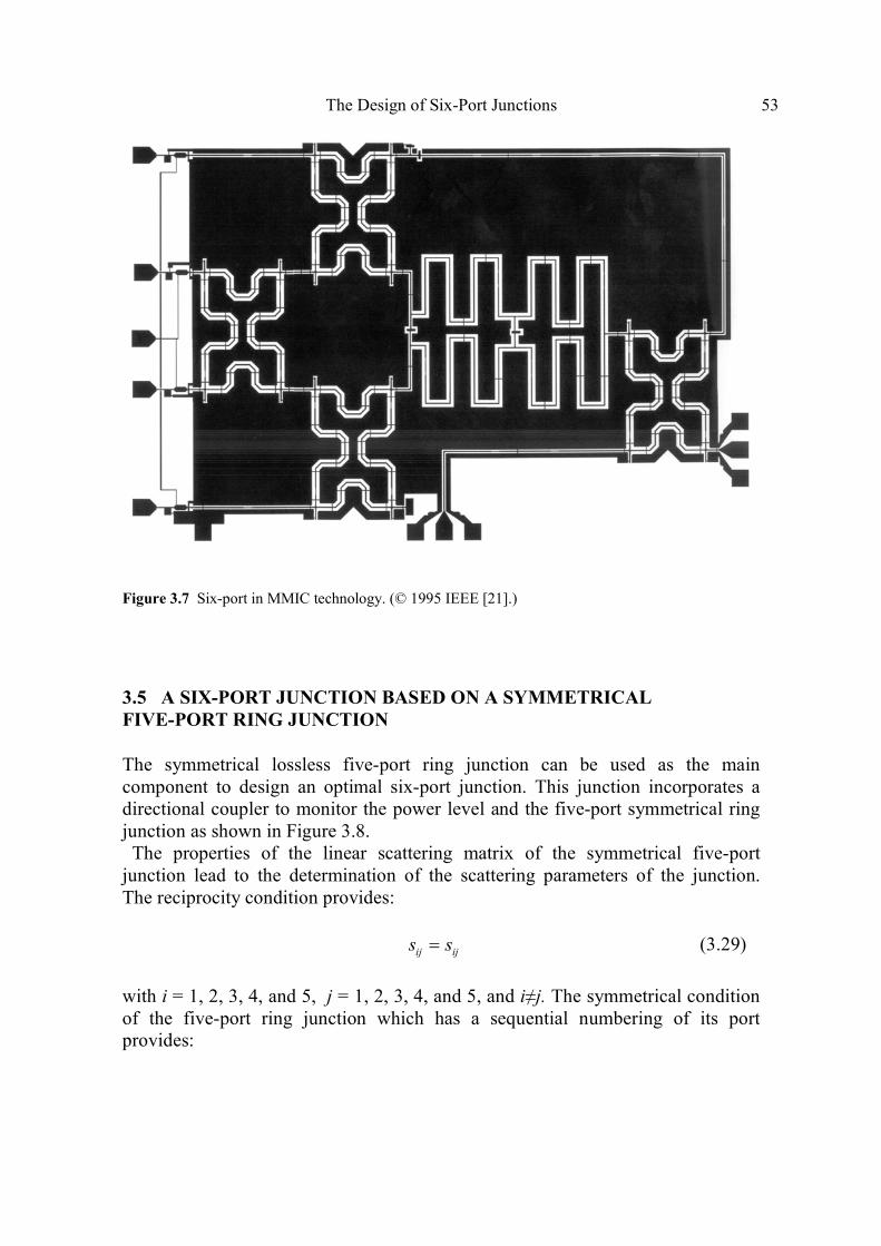
The Design of Six-Port Junctions 53
Figure 3.7 Six-port in MMIC technology. (© 1995 IEEE [21].)
3.5 A SIX-PORT JUNCTION BASED ON A SYMMETRICAL
FIVE-PORT RING JUNCTION
The symmetrical lossless five-port ring junction can be used as the main
component to design an optimal six-port junction. This junction incorporates a
directional coupler to monitor the power level and the five-port symmetrical ring
junction as shown in Figure 3.8.
The properties of the linear scattering matrix of the symmetrical five-port
junction lead to the determination of the scattering parameters of the junction.
The reciprocity condition provides:
ij ijs s= (3.29)
with i = 1, 2, 3, 4, and 5, j = 1, 2, 3, 4, and 5, and i≠j. The symmetrical condition
of the five-port ring junction which has a sequential numbering of its port
provides:

54 The Six-Port Technique with Microwave and Wireless Applications
(a)
(b)
Figure 3.8 (a) Schematic of a symmetrical five-port ring junction. (b) A schematic of a symmetrical five-port ring based six-port junction.

The Design of Six-Port Junctions 55
11 22 33 44 55s s s s s= = = = = α (3.30a)
12 15 23 34 45s s s s s= = = = = β (3.30b)
13 14 24 25 35s s s s s= = = = = δ (3.30c)
From (3.30) one can conclude that only three independent s parameters are
sufficient to form the S matrix:
α β δ δ β β α β δ δ = δ β α β δ δ δ β α β
β δ δ β α
S (3.31)
For a lossless junction, one can write that
2 2 22 2 1α + β + δ = (3.32)
The unitary condition of S matrix provides
2
2
2
2
0
0
0
0
∗ ∗ ∗ ∗
∗ ∗ ∗ ∗
∗ ∗ ∗ ∗
∗ ∗ ∗ ∗
αβ + βα + δβ + βδ + δ =αδ + δα + δβ + βδ + β =
αδ + βδ + δβ + δα + β =
αβ + βδ + δβ + βα + δ =
(3.33)
For a matched five-port ring junction ( 0α = ), using (3.32) and (3.33) leads to
2
2
2 2
0
0
2 2 1
∗ ∗
∗ ∗
δβ + βδ + δ =
δβ + βδ + β =
β + δ =
(3.34)
56 The Six-Port Technique with Microwave and Wireless Applications
The above set of equations gives:
0.5β = δ = (3.35)
By assuming that β is real and by substituting the value of β in one of the two
first equations, one can easily deduce that:
0.5 120δ = ∠ ± (3.36)
Finally, the S matrix of a six-port junction comprising a symmetrical and matched
five-port ring junction and an ideal directional coupler connected to port 1 of the
five-port junction as shown in Figure 3.8 is as follows:
0
0 0
0 0 0 0 0
0 0
0 0
0 0
t jc t t t
t
jc
t
t t
t t
δ β δ β δ β β δ
= β β δ δ
δ β δ β
β δ δ β
spS
(3.37)
Using (1.13), one can deduce the positions of the three iq points in the complex
plane using the S parameters of the six-port junction:
41
4
21 42
2 60s t
qs s t
β= = = ∠
− − δβ (3.38a)
51
5
21 52
2 180s t
qs s t
δ= = = ∠
− − δβ (3.38b)
and
61
6 2
21 62
2 60s
qs s
β= = = ∠ −
− −δ (3.38c)
These values were calculated using 0.5 120δ = ∠ . The analytical development to
obtain the above design specifications can be found in [10]. An optimal L-band
microstrip line six-port junction designed on a 10 mil Alumina substrate, shown in
Figure 3.9, is reported in [22]. It incorporates a 10 dB edge-line coupler and the
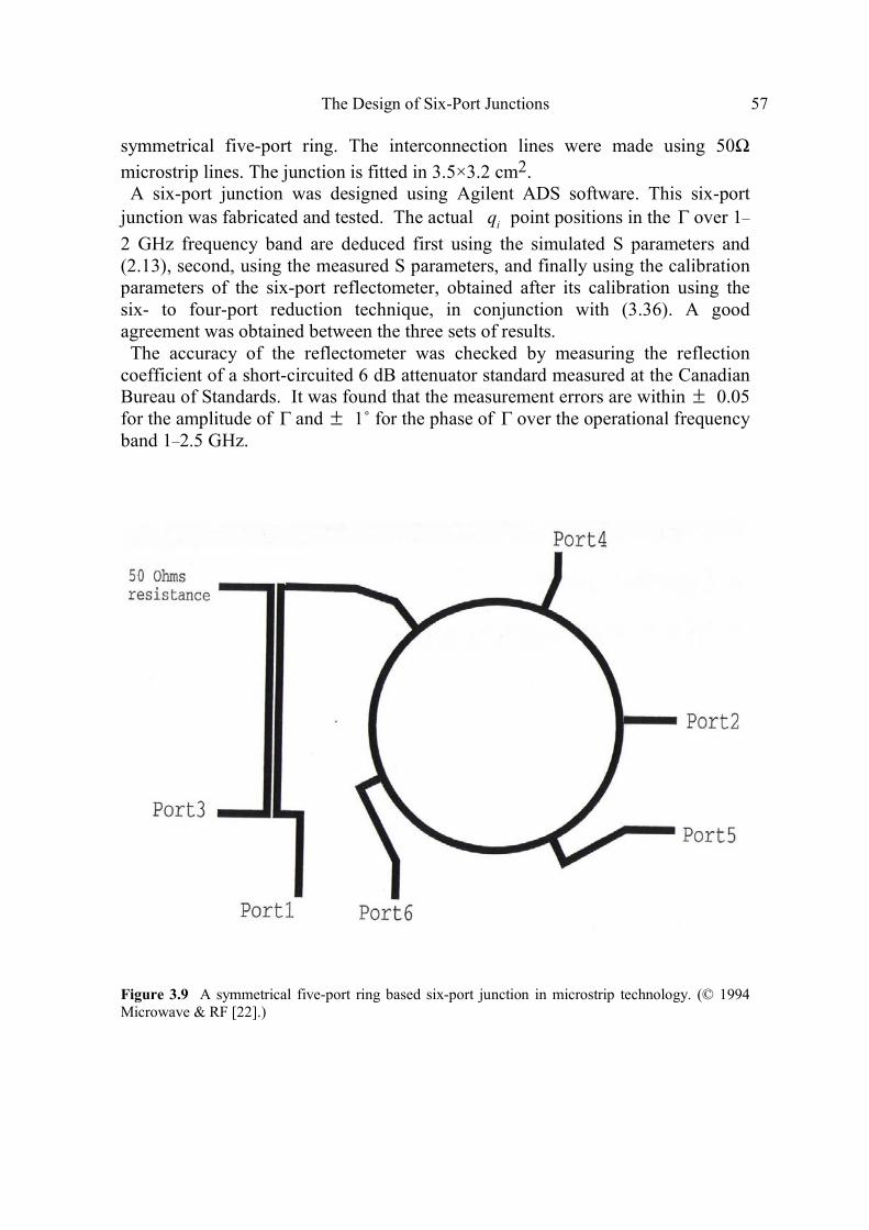
The Design of Six-Port Junctions 57
symmetrical five-port ring. The interconnection lines were made using 50Ω
microstrip lines. The junction is fitted in 3.5×3.2 cm2.
A six-port junction was designed using Agilent ADS software. This six-port
junction was fabricated and tested. The actual iq point positions in the Γ over 1–
2 GHz frequency band are deduced first using the simulated S parameters and
(2.13), second, using the measured S parameters, and finally using the calibration
parameters of the six-port reflectometer, obtained after its calibration using the
six- to four-port reduction technique, in conjunction with (3.36). A good
agreement was obtained between the three sets of results.
The accuracy of the reflectometer was checked by measuring the reflection
coefficient of a short-circuited 6 dB attenuator standard measured at the Canadian
Bureau of Standards. It was found that the measurement errors are within ± 0.05
for the amplitude of Γ and ± 1˚ for the phase of Γ over the operational frequency
band 1–2.5 GHz.
Figure 3.9 A symmetrical five-port ring based six-port junction in microstrip technology. (© 1994
Microwave & RF [22].)

58 The Six-Port Technique with Microwave and Wireless Applications
3.6 HIGH POWER SIX-PORT JUNCTION IN HYBRID WAVEGUIDE/
STRIPLINE TECHNOLOGY
A high power six-port junction in hybrid waveguide stripline technology, using a
stripline waveguide directional coupler and a nonsymmetrical stripline five-port
ring junction, was designed and manufactured and tested at 2.45 GHz (ISM
frequency). This junction is capable of handling power as much as the waveguide
portion of the junction could handle. It is expected that this design could handle
up to several kilowatts of power; the details of the design can be found in [23].
The block diagram is shown in Figure 3.10.
Figure 3.10 A high power six-port junction comprising a nonsymmetrical five-port ring junction in
microstrip technology and hybrid stripline-waveguide directional coupler. (© 1994 IEEE [23].)

The Design of Six-Port Junctions 59
3.7 WORST-CASE ERROR ESTIMATION
It was shown in Chapter 2 that the six-port reflectometer can be linearly modeled
by a 4×4 real matrix and the basic relation that governs its operation in (2.17) is
repeated hereafter:
= ρ ΓP C (3.39)
Also, it was shown that the calculation of the real and imaginary parts of the
reflection coefficient can be realized by means of (2.19) repeated hereafter
4
3 2
1
4
1 2
1
j jj
j jj
x P
Rx P
+=
+=
=∑
∑ and
4
4 2
1
4
1 2
1
j jj
j jj
x P
Ix P
+=
+=
=∑
∑ (3.40)
In Chapter 2, it was shown that the iq values of the six-port junction are related to
the entries of matrix C by means of (2.18).
For a six-port junction that incorporates a reference port (port 3) to monitor the
power level and which is completely isolated from the measuring port ( )320s ≅ ,
and if the measuring port mismatch is not excessive ( )220s ≅ , the module of
3q
becomes too large and the six-port junction is almost completely defined by the
position of the three remaining 4q , 5q , and
6q . In such a case, the first row
elements of C can be approximated by 11 1c = and 12 13 14 0c c c= = = .
Figure 3.11 shows a geometrical representation of the different parameters
involved in the worst case error estimation. Using some geometrical
manipulations, it is simple to show that the expression of the relative error in
amplitude measurements and the absolute error in phase measurements, in the
worst-case situation, can be calculated using the absolute errors of the real and
imaginary parts, R∆ and I∆ of the reflection coefficient jR IΓ = Γ ∠ϕ = + , as
follows:
max ,r b
Γ − Γ Γ − Γ∆ Γ = Γ Γ Γ
(3.41a)
( )max ,n v∆ϕ = θ θ (3.41b)
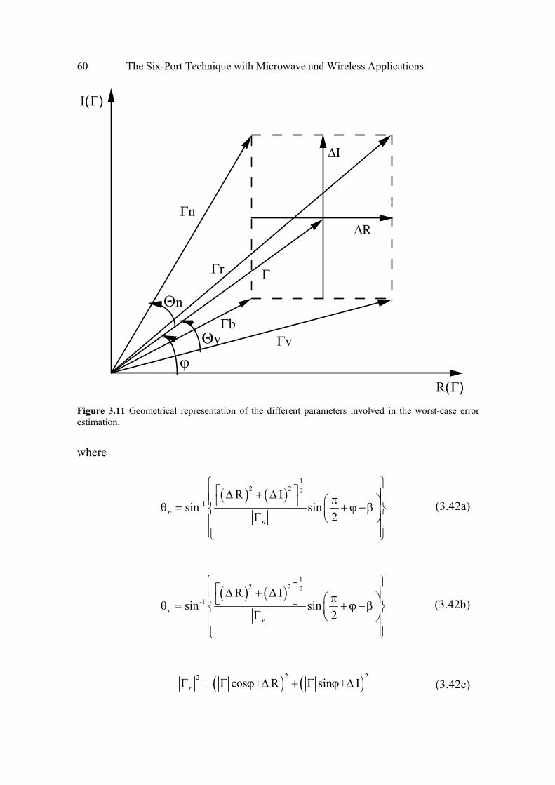
60 The Six-Port Technique with Microwave and Wireless Applications
R(Γ)
I(Γ)
∆R
∆I
Γv
Γn
Γb
Γr Γ
ϕ
Θv
Θn
Figure 3.11 Geometrical representation of the different parameters involved in the worst-case error
estimation.
where
( ) ( )1
2 2 2
-1R I
sin sin2
n
n
∆ + ∆ π θ = + ϕ −β Γ
(3.42a)
( ) ( )1
2 2 2
-1R I
sin sin2
vv
∆ + ∆ π θ = + ϕ − β Γ
(3.42b)
( ) ( )2 22
cos + R sin + IrΓ = Γ ϕ ∆ + Γ ϕ ∆ (3.42c)

The Design of Six-Port Junctions 61
( ) ( )2 22
cos + R sin IvΓ = Γ ϕ ∆ + Γ ϕ − ∆ (3.42d)
( ) ( )2 22cos R sin + InΓ = Γ ϕ − ∆ + Γ ϕ ∆ (3.42e)
( ) ( )2 22cos R sin IbΓ = Γ ϕ − ∆ + Γ ϕ − ∆ (3.42f)
and
-1 Rtan
I
∆ β = ∆
(3.42g)
Using (3.41), we can deduce the expression of the absolute errors of the real and
imaginary parts of Γ as a function of the parameters of the six-port junction and
the relative errors in the power readings as follows:
6
i=3
RR = i i
i
PP
∂∆ α
∂∑ (3.43a)
and
6
i=3
II = i i
i
PP
∂∆ α
∂∑ (3.43b)
where
( )4
3, 2 1 1, 2 3 2
1
24
1 2
1
Ri j i j j
j
i
j jj
x x x x P
Px P
− − +=
+=
−∂
=∂
∑
∑
(3.44a)

62 The Six-Port Technique with Microwave and Wireless Applications
( )4
4, 2 1 1, 2 4 2
1
24
1 2
1
Ii j i j j
j
i
j jj
x x x x P
Px P
− − +=
+=
−∂
=∂
∑
∑
(3.44b)
and
ii
i
P
P
∆α = , i=3, 4, 5, and 6 (3.44c)
To estimate the worst-case error in reflection coefficient measurements for a given
six-port junction, it is sufficient to know the values of the iq positions and the
relative errors of the power detectors. The above formulation can be used to
compare different six-port junction configurations, such as Engen’s design or
quasi-optimal design or other designs. A comparative study of some proposed
six-port junction designs has been carried out in [24]. Constant contour plots, for
amplitude and phase measurements, in the worst-case situation, have been
obtained over the entire Smith chart and for different precision of power sensors.
It was found that a dynamic range of 60 dB can be reached with a power sensor
having a precision of 0.1%.
References
[1] Engen, G. F., “An Improved Circuit for Implementing the Six-Port Technique of Microwave
Measurements,” IEEE Trans. on Microwave Theory & Tech., Vol. MTT 25, No. 12, pp. 1080–1083, December 1977.
[2] Griffin, E. J., “Six-Port Reflectometer Circuit Comprising Three Directional Coupler,” Electron Letts., pp. 491–493, 1982.
[3] Rafal, M. D., and Joines, W. T., “Optimizing the Design of the Six-Port Junction,” IEEE MTT-S Digest, pp. 437–439, 1980.
[4] Collier, R. J., and N. A. Deeb, “"On the Use of a Microstrip Three Line System as a Six-Port Reflectometer,” IEEE Trans. on Microwave Theory & Tech., Vol. MTT-27, pp. 847–853,
October 1979.
[5] Cullen, A. L., “Impedance Measurement Using Six-Port Directional Coupler,” IEE Proc., Vol. 127, Part H, No. 2, pp. 32–38, April 1980.
[6] Hansson, E. R. B., and G. P. Riblet, “An Ideal Six-Port Network Consisting of Matched
Reciprocal Losses Five-Port and a Perfect Directional Coupler,” IEEE Trans. on Microwave Theory & Tech., Vol. 31, pp. 284–289, March 1983.
[7] Eda, K., “Miniature Hybrid Microwave IC’s Using Novel Thin Film Technology,” MTT-S, International Microwave Symposium Digest, pp. 419–422, 1990.

The Design of Six-Port Junctions 63
[8] Ghannouchi, F. M., S. Wang, and R. G. Bosisio, “A Preferred Frequency Balanced Six-Port
Junction in Microstrip Line,” SMBO International Microwave Symposium Proceedings, Vol. 1, pp. 285–290, July 1989.
[9] Cullen A. L., and A. J. Belfort, “Seven Port Millimeter-Wave Reflectometer,” Electronics Lett., Vol. 21, No. 3, January 1985.
[10] Riblet G. P., and E. R. B. Hansson, “An Ideal Six-Port Network Consisting of a Matched
Reciprocal Lossless Five-Port and a Perfect Directional Coupler,” IEEE Tran. on Microwave Theory & Tech., Vol. MTT-31, No. 3, pp. 284–288, 1983.
[11] Robert, P. J., and J. E. Carroll, “Design Features of Multi-Port Reflectometers,” IEE Proc., Vol.
129, Pt. H, No. 5, pp. 245–252, October 1982.
[12] Li, S. H., and R. G. Bosisio, “Analysis and Optimized Circuit of Six-Port Reflectometer,” Acta Electronica Sinica, Vol. 11, No. 2, pp. 1–8, 1983.
[13] Wang, S., “A CAD/CAM Wideband Microwave Six-Port Junction,” Master thesis, École Polytechnique de Montreal, February 1990.
[14] Griffin, E. J., G. J. Slack, and L. D. Hill, “Broadband Six-Port Reflectometer Junction,” Electron Lett., pp. 921–922, 1983.
[15] Feng, Z. H., “Broadband Dielectric Waveguide Coupler and Six-Port Network,” IEEE MTT-S Digest, pp. 237–240, 1986.
[16] Malkomes, M., and R. Walsdorf, “Integrated Fin-Line 6-Ports for MM-Wave Network
Analyzers,” IEEE MTT-S Digest, pp. 669–671, 1986.
[17] Ohta, I., “A New Six-Port Microwave Network: Six-Port Magic Junction,” IEEE Tran. on Microwave Theory & Tech., Vol. MTT-36, pp. 859–864, May 1988.
[18] Berman, M., P. I. Somlo, and M. J. Buckley, “A Comparative Statistical Study of Some Proposed Six-Port Junction Designs,” IEEE Trans. on Microwave Theory & Tech., Vol. MTT-35, pp. 971–
977, November 1987.
[19] Ghannouchi, F. M., R. G. Bosisio, and S. Wang “A CAD/CAM of an Optimum and Wideband Triplate Six Port Junction,” International Conference on Millimeter Wave & Microwave
(ICOMM-90), Dehra Dun, India, pp. 466–470, December 1990.
[20] Ghannouchi, F. M., R. G. Bosisio, D. Maurin, and M. Cuhaci, "A Design of Six-Port Junction on
MHMIC Technology,” Microwave and Optical Tech. Letters, Vol. 6, No.10, pp. 573–575,
August 1993.
[21] Taymia, S. I., R. Hajji, and F. M. Ghannouchi, “A CAD/CAM of an Coplanar Wave Guide
MMIC Six-Port Junction,” Canadian Conference in Electrical and Computer Engineering, Montreal Canada, September 1995.
[22] Ghannouchi, F. M., “Compact Microwave Circuit Perform Swept Vector Measurements,”
Microwave & RF, pp. 67–68, February 1994.
[23] Akyel, C., F. M. Ghannouchi, and M. Caron, “A New Design for High-Power Six-Port Reflectometers Using Hybrid Stripline/Waveguide Technology,” IEEE Trans. on Instrumentation and Measurements, Vol. 43, No. 2, pp. 316–321, April 1994.
[24] Ghannouchi, F. M., and R. G. Bosisio, “A Comparative Worst-Case Error Analysis of Some Proposed Six-Port Designs,” IEEE Trans. on Instrumentation and Measurements, Vol. 37, No. 4,
pp. 552–556, 1988.


65
Chapter 4
Calibration Techniques
In Chapter 2, the fundamentals of the six-port techniques have been presented and
it has been shown that a calibration procedure to determine the parameters of the
model of the six-port reflectometer is needed. Different methods have been
proposed in the literature [1–14]. The number of known standards and the
computation effort required are the most important parameters in selecting a
calibration technique. Two categories of methods can be defined. The first
category uses a linear formalism to solve for the calibration parameters, and the
second category uses nonlinear formalism in conjunction with iterative numerical
techniques to solve for the calibration parameters. In this chapter we will present
five different calibration techniques as well as a calibration technique to increase
the dynamic range of the six-port reflectometer. A calibration technique using
active loads will be also presented.
4.1 CALIBRATION METHOD USING SEVEN STANDARDS
It was shown in Chapter 2 that the three normalized power readings are related to
reflection coefficient of a DUT, Γ , as follows:
2
i i
3 1i
d ep
c
Γ +=
Γ +i =4, 5, and 6 (4.1)
By designating x jyΓ = + , 3 3 3x yc c jc= + , i xi yid d jd= + , and i xi yie e je= + , and
after algebraic manipulations, (4.1) can be written as follows:
( ) ( )( )( ) ( )
2 2 2
3 3 3
2 22 2
1 2
2
i x y
i i i i
p c x y c x c y
d x y e x y
+ + + − =
+ + + η + κ, i = 4, 5, and 6 (4.2)

66 The Six-Port Technique with Microwave and Wireless Applications
where i xi xi yi yid e d eη = + and i xi yi yi xid e d eκ = − . The connection of a well-
known standard having a reflection coefficient, kΓ , to the measuring port of the
six-port reflectometer gives
( ) ( ) ( ) ( )2 2 22 2 2 2
3 3 3
11 2 2k k x k y k i k k i i k i k
ik
c x y c x c y d x y e x yp
+ + + − = + + + η + κ
for i = 4, 5, and 6 (4.3)
As we have mentioned before, the determination of the relative values of the
calibration parameters is sufficient because the formalism that relates the
reflection coefficient, Γ , to the calibration parameters is power independent; thus,
one can deliberately set the value of the amplitude of c3 to unity (3 1c = ) .
It is important to notice that for a given standard k, (4.3) provides only two
independent equations, because the left-hand side of (4.3) is the same for the three
equations. Therefore, seven standards are required to solve for the 14 real linearly
independent calibration parameters2
id ,2
ie , 3xc , cy3 , iη , and iκ .
Alternatively, one can solve the set of 14 equations, obtained using (4.3) and
seven standards, as a nonlinear set of 14 equations comprising fourteen
independent unknowns 3 3, , , ,x y xi yi xic c d d e , and yie ; i= 4, 5, and 6. Writing (4.2)
for i and j with i≠j and subtracting these equations, one can easily deduce that
2 2 ij ij ij
ij
ep p x p yx y
dp
+ η + κ+ =
− (4.4)
Where
22
jiij
i j
eeep
p p= − ,
22
jiij
i j
dddp
p p= − ,
22
2ji
iji j
pp p
ηη η = −
, and
22
2ji
iji j
pp p
κκ κ = −
for i = 4, 5, and 6; j = 4, 5, and 6 and i ≠ j .
Equation (4.4) leads to a set of two linear and independent equations in x and y
( ) ( )( ) ( )
46 45 45 45 45 46 46 46
56 45 45 45 45 56 56 56
dp ep p x p y dp ep p x p y
dp ep p x p y dp ep p x p y
+ η + κ = + η + κ
+ η + κ = + η + κ
(4.5)

Calibration Techniques 67
The calculation of the real and imaginary parts of the reflection coefficient Γ of
any DUT connected to the measuring port uses the three relative power readings
and the calibration parameters as follows:
( )( )( )( )( )( )( )( )
45 56 56 45 56 46 46 56
46 56 56 46 56 54 45 56
56 45 45 56 56 46 46 56
56 46 46 56 56 56 45 56
ep dp ep dp p dp p dp
ep dp ep dp p dp p dpx
p dp p dp p dp p dp
p dp p dp p dp p dp
− κ − κ −
− κ − κ = η − η κ − κ −
η − η κ − κ
(4.6a)
and
( )( )( )( )( )( )( )( )
56 45 45 56 46 56 56 46
45 56 56 45 56 46 46 56
56 45 45 56 56 46 46 56
56 46 46 56 56 56 46 56
p dp p dp ep dp p dp
ep dp ep dp p dp p dpy
p dp p dp p dp p dp
p dp p dp p dp p dp
η − η − κ −
− η − η = η − η κ − κ −
η − η κ − κ
(4.6b)
This method requires a large number of well-known standards. The imprecision
in the knowledge of their reflection coefficients has a direct effect on the accuracy
of the calculation of the calibration parameters, consequently the accuracy of the
reflection coefficient measurements. Therefore, it is more interesting, in practice,
to minimize the number of the known calibration standards required in the
calibration procedure. For this reason a calibration technique that requires only
five standards is reported in the next section.
4.2 LINEAR CALIBRATION USING FIVE STANDARDS
It was shown in Chapter 2 that the six-port reflectometers can be modeled by a
(4×4) real matrix, C, which relates the four power readings to the complex
reflection coefficient Γ as follows:
= ρ ΓP C (4.7)
where [ ]3 4 5 6, , ,T
p p p p=P , 2
1 Re( ) Im( )T
= Γ Γ Γ
Γ , and 2
2bρ = . By
connecting four different standards to the measuring port, one can write in an
explicit manner:

68 The Six-Port Technique with Microwave and Wireless Applications
3 31 32 33 34
2
4 41 42 43 44
5 51 52 53 54
6 61 62 63 64
1
Re( )
Im( )
k
k kk
k k
k k
p c c c c
p c c c c
p c c c c
p c c c c
Γ = ρ Γ Γ
k=1, 2, 3, and 4 (4.8)
By dividing each row of the above matrix equation by the first row one can
obtain:
( ) ( )
( ) ( )( )
2
1 2 3 4
2
31 32 33 34
3
Re Im
Re Im
j j k j k j k
jkk k k
k
c c c c
pc c c c
p
+ Γ + Γ + Γ =
+ Γ + Γ + Γ (4.9)
with j = 4, 5, and 6 designating the power readings and k = 1, 2, 3, and 4
designating the calibration standards.
The above equations can be written in matrix format as follows
− −= 1 1
j 3j 3C G P P GC (4.10)
where 1 2 3 4, ,
T
j j j jc c c c = jC
2
1 1 1
2
2 2 2
2
3 3 3
2
4 4 4
1 Re( ) Im( )
1 Re( ) Im( )
1 Re( ) Im( )
1 Re( ) Im( )
Γ Γ Γ Γ Γ Γ
= Γ Γ Γ
Γ Γ Γ
G
1
2
3
4
0 0 0
0 0 0
0 0 0
0 0 0
j
j
j
j
p
p
p
p
=
jP
Using (4.10), it can be easily deduced that
4 5 64 5 6
− − − −= = = =1 1 1 1
3 3 0P GC P GC P GC P GC V (4.11)
where 1 2 3 4
1 1 1 1, , ,
T
= ρ ρ ρ ρ 0
V is an unknown vector related to the power flow
exciting the four standards during calibration procedure. Equation (4.11) leads to
−= 1
jj 0C G P V , j=3, 4, 5, and 6 (4.12)
After connecting a fifth standard to the measuring port, one can write

Calibration Techniques 69
5 55 53 4 5 6
, , ,T
= ρ Γ = ρ Γ 5P C C C C C (4.13)
Substituting (4.12) in (4.13), one can write
5 3 4 5 6 5, , ,
T− − − − = ρ Γ 1 1 1 1
5 0 0 0 0P G P V G P V G P V G P V (4.14)
Rearranging (4.14), one can write
5 3 4 5 6, , ,
T T T T = ρ 5 0 0 0 0P V P V P V P V P S (4.15)
where [ ]5, , ,
T Ta b c d− = Γ =
1S G is a known vector which can be calculated
using the five reflection coefficients of the five calibration standards. Equation
(4.15) can be written in an explicit manner as follows
35 31 32 33 34 5 1
45 41 42 43 44 5 2
55 51 52 53 54 5 3
65 61 62 63 64 5 4
p p a p b p c p d
p p a p b p c p d
p p a p b p c p d
p p a p b p c p d
ρ ρ ρ ρ = ρ ρ
ρ ρ
(4.16)
The solution of the above matrix equation leads to the calculation of the relative
values of the entries of vector5ρ
0V . It was mentioned in Chapter 1 that the
formalism to calculate the reflection coefficient is power level independent;
therefore, the proportionality constant 5ρ has no effect on the overall final results
since it is automatically embedded in the calibration parameters ijc .
Knowing 5ρ
0V and using (4.12), one can deduce all the entries of the calibration
matrix C. The calculation of the reflection coefficient for any DUT is as follows
( )
4
3 2
1
4
1 2
1
Re ,
j jj
j jj
x P
x P
+=
+=
Γ =∑
∑ ( )
4
4 2
1
4
1 2
1
Im
j jj
j jj
x P
x P
+=
+=
Γ =∑
∑ (4.17)
where xij are the entries of the inverse of the calibration matrix C. The power
absorbed by the DUT can be calculated as follows:

70 The Six-Port Technique with Microwave and Wireless Applications
( ) ( )4
2 2 2
2 1 2
1
1 1DUT DUT DUT j jj
P b x P +=
= − Γ = − Γ
∑ (4.18)
4.3 NONLINEAR CALIBRATION USING FOUR STANDARDS
It was shown in Chapter 1 that the calibration matrix of the six-port reflectometers
is the following:
( ) ( )( ) ( )( ) ( )( ) ( )
22 2 2 2
3 3 3 3 3 3 3
22 2 2 2
4 4 4 4 4 4 4
22 2 2 2
5 5 5 5 5 5 5
22 2 2 2
6 6 6 6 6 6 6
2 Re 2 Im
2 Re 2 Im
2 Re 2 Im
2 Re 2 Im
q q q
q q q
q q q
q q q
α α − α − α α α − α − α
= α α − α − α α α − α − α
C (4.19)
One can deduce from (4.19) that the elements of each row are related by the
following equation:
2 2
3 4 1 24 0j j j jc c c c+ − = , j = 3, 4, 5, and 6 (4.20)
On the other hand, it was also shown that
= j
j 3C H C ; j = 3, 4, 5, and 6 (4.21)
where − −=j 1 1
j 3H G P P G and G is a known matrix related to the four reflection
coefficients of the four standards and their corresponding power readings. As we
have mentioned before, the knowledge of the relative values of the entries of the
calibration matrix of the six-port reflectometer is sufficient to perform
measurements since the measurement equation is power independent. Therefore,
without any constraint, we can fix c11 to unity.
The substitution of (4.21) into (4.20) and the writing of results in explicit manner
give
2 2 2
1 2 32 3 33 4 34 23 32 33 24 32 34
34 33 34 12 32 13 33 14 34
2(
) 0
j j j j j j
j j j j
c c c c c c c
c c c c c
δ + δ + δ + δ + σ + σ +
σ + σ + σ + σ = (4.22)

Calibration Techniques 71
where j 2 2
3 4 1 2( ) ( ) 4j j j ji i i i ih h h hδ = + − , and
3 3 4 4 1 2 2 12( ),j j j j j j j j jik i k i k i k i kh h h h h h h hσ = + − +
with j = 3, 4, 5, and 6.
Equation (4.22) is a set of four nonlinear equations comprising three unknowns:
32c , 33c , and
34c . In practical situations, the six-port junction incorporates a
reference port, port 3, to monitor the power level; hence, the power reading 3P is
quasi-independent of the DUT. In such a case the entries of the first row can be
approximated by31 1c ≈ , and
32 33 34 0c c c≈ ≈ ≈ . These values can be used as
initial guests for the numerical algorithm needed to calculate the actual values of
the three unknowns. The Newton-Raphson technique can be used for this purpose.
Following the calculation of the entries of the first row of the C matrix, the values
of the entries of the remaining rows can be straightforwardly calculated using
(4.10). The calculation of the reflection coefficient of any DUT is then obtained
using (4.17).
All the calibration and measurement methods described above require the use of
well-known standards and relate explicitly in one step the reflection coefficient Γ
to the power readings and the calibration parameters. The calibration and
measurement procedures based on the six- to four-port reduction technique and
the concept of de-embedding are more powerful and robust, in practice, since they
require only three well-known standards.
4.4 NONLINEAR CALIBRATION USING THREE STANDARDS
It was mentioned in Chapter 1 that 11 real parameters are sufficient to model the
six-port reflectometer. It also was mentioned that the embedded reflection
coefficient, 4w , can be related to the reflection coefficient, Γ , via the three error
box complex parameters (six real parameters). This is shown in Figure 4.1.
Consequently, the partition of the calibration in two different steps is possible.

72 The Six-Port Technique with Microwave and Wireless Applications
Figure 4.1 Modeling of a six-port reflectometer; (a) an actual six-port reflectometer, and (b) an ideal
reflectometer followed by a two-port error box network.
The first step is to find five real parameters that relate the four power readings to
the embedded reflection coefficient, 4w , and the second step is to find in the error
box, three complex parameters, , ,and ,c d e which relate, 4w to Γ via a bilinear
transformation. By defining
-
4mjw w e ϕ= (4.24)
Equation (2.29) becomes
2
4p w= (4.25)
Actual Reflectometer
Ideal
ReflectometerError Box
w 4 Γ
Six-Port Reflectometer
Γ(a)
(b)

Calibration Techniques 73
2
5 2
5
1p w m
A= − (4.26)
( ) 2
6 2
6
1n mjp w n e
Aϕ −ϕ= − (4.27)
We notice that the second iQ point in the W plane becomes real following the
bilinear mapping. The graphical common intersection of these circles in the W
plane gives the de-embedded reflection coefficient w shown in Figure 4.2.
Equations (2.32) and (2.33) give explicit expressions for the calculation w 4 and
can be used to calculate w providing that we substitute mm ∠ϕ and nn ∠ϕ by
0m ∠ and ( )n mn ∠ ϕ − ϕ in (2.33), respectively. Therefore, the real and
imaginary parts of the embedded reflection coefficient w can be calculated as
follows:
Figure 4.2 Graphical solution in the W plane.
Re (W)
Im (W)
m
n
| n |
0
| m | . .
.
A5p
5¦
¦ p 4
¦ 6
A6
p
ϕ m
ϕn -
w

74 The Six-Port Technique with Microwave and Wireless Applications
( )2 2
4 5 5Re2
p A p mw
m
− += (4.28)
( )( )
( )( )( )
( )
22 2 24 6 6 n 4 5 5
n m n m
cos Im
2 sin 2 sin
mp A p n p A p m
wn m
− + ϕ − ϕ − += +
ϕ − ϕ ϕ − ϕ (4.29)
Knowing that ( )( ) ( )( )2 22
4 Re Imp w w w= = + and using (4.28) and (4.29), one
can eliminate w and obtain a nonlinear equation function only of the power
readings and the five calibration parameters as follows:
( ) ( ) ( )( )( )
222 2 22 2 2 2 2 2
4 5 5 4 6 6 4
22 2 2
4 5 5 4 6 6
4 1
2 0
n p A p m m p A p n m n p z
m n p A p m p A p n z
− + + − + − −
− − + − + = (4.30)
where ( )n mcos z = ϕ − ϕ . Equation (4.30) is the basis of six- to four-port
reduction techniques. At least five different and unknown loads are required to
generate a system of five equations in order to solve for the five calibration
parameters 5 6, , ,A A m n , and z.
It is clear from the (4.30) that the solution, 0m n= = , is the trivial one to avoid,
since (4.30) will be equal to zero regardless of the values of the normalized power
readings, 4p , 5p , and
6p or the parameters 5A and
6A . The calculation of the de-
embedded reflection coefficient w as a function of the power readings and the five
calibration parameters are as follows:
( )2 2
4 5 5Re2
p A p mw
m
− += (4.31a)
( )( )2 2 22
4 5 54 6 6
2
1Im
2 21
z p A p mp A p nw
n mz
− +− +± = + −
(4.31b)
The sign ambiguity can be resolved using a partially known reflection coefficient.
To obtain a good estimation of the embedded reflection coefficient, w, one can
calculate the common intersection of the three radical axes as shown in Figure 4.3.

Calibration Techniques 75
Figure 4.3 Common intersections of the three straight lines in the W complex plane.
Each straight line passes through the two common intersections of one pair of
circles among the three pairs. This intersection is the radical center, cr , of the
three circles, and its coordinates are:
( )
2 2 2
0Re2
mc
r r mr
m
− += (4.32a)
( )22 2 2
0 2Re( ) 1Im
2
n cc
r r n r n zr
z n
− + − −= (4.32b)
m
o
n
rm
rn
ro
Radical center
Φn
--Φ
m

76 The Six-Port Technique with Microwave and Wireless Applications
where
2
0 4r p= is the square of the first circle; 2 2
5 5mr A p= is the square of the
second circle, and 2 2
6 6nr A p= is the square of the third circle.
In practice, the intersection of the three circles is not a clear point, but a small
curvilinear triangle where the “true” embedded reflection coefficient should fall as
shown in Figure 4.2. Equation (4.32) can be used to calculate an estimate of w. This estimate can be used as an initial guess for further iterative calculations to
obtain the actual embedded reflection coefficient, w.
For the omn triangle in Figure 4.3, it easy to deduce that:
( )2 2 2
n mcos 2
n m n mz
nm
+ − −= ϕ − ϕ =
(4.33)
By substituting (4.33) into (4.30), one can obtain an equivalent equation identical
to the one published in [12, 15, and 16] as follows:
( ) ( )( ) ( ) ( )( )
2 4 2 4 2 2 2
4 5 5 6 6 5 4 5 6 4 6
2 2 2
5 6 5 6 4 5 5
2
6 6 0
pp qA p rA p r p q A p p q p r A p p
p q r A A p p p p q r p q q p r A p
r r p q A p pqr
+ + + − − + − −
+ − − + − − + − − +
− − + =
(4.34)
where2
p n m= − , 2
q n= and 2
r m= .
By introducing new variables, (4.34) can be linearized as follows [15]:
2 2 2
1 4 2 5 3 6 4 4 5 5 5 6 6 5 6
7 4 8 5 9 6 1
x p x p x p x p p x p p x p p
x p x p x p
+ + + + +
+ + + = − (4.35)
where
1 1x qr= (4.36a)
4
2 5x A pr= (4.36b)
4
3 6x A pq= (4.36c)
( ) 2
4 5x r p q A pqr= − − (4.36d)

Calibration Techniques 77
( ) 2
5 6x q p r A pqr= − − (4.36e)
( ) 2 2
6 5 6x p q r A A pqr= − − (4.36f)
( )7x p q r qr= − − (4.36g)
( ) 2
8 5x q p r A pr= − − (4.36h)
26
9
( )r p q Ax
pq
− −= (4.36i)
In practice, nine or more different and unknown loads are needed to solve a linear
system that can be formed using (4.35). The value obtained can be used to
calculate an initial guess for the nonlinear system to be solved in the least squares
sense as follows [15].
5 7 9
1 9 5 7
2
2
x x xr
x x x x
−=
− (4.37a)
4 7 8
1 8 4 7
2
2
x x xq
x x x x
−=
− (4.37b)
5 7 9 4 7 8 7
1 9 5 7 1 8 4 7 1
2 2
2 2
x x x x x x xp
x x x x x x x x x
− −= + +
− − (4.37c)
1
45 7 9 4 7 8 7 5 7 9
5 2
1 9 5 7 1 8 4 7 1 1 9 5 7
2 2 2
2 2 2
x x x x x x x x x xA x
x x x x x x x x x x x x x
− − −= + + − − −
(4.37d)
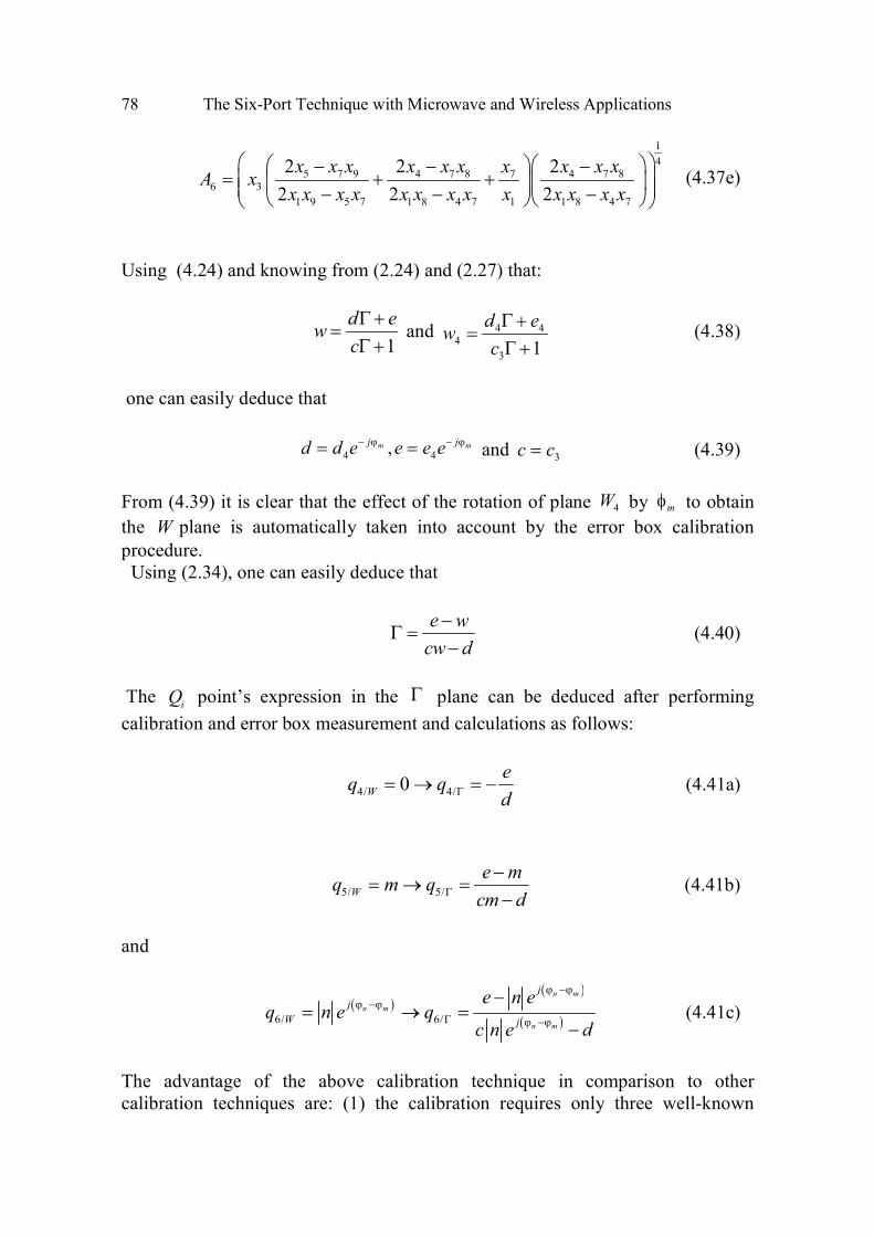
78 The Six-Port Technique with Microwave and Wireless Applications
1
45 7 9 4 7 8 7 4 7 8
6 3
1 9 5 7 1 8 4 7 1 1 8 4 7
2 2 2
2 2 2
x x x x x x x x x xA x
x x x x x x x x x x x x x
− − −= + + − − −
(4.37e)
Using (4.24) and knowing from (2.24) and (2.27) that:
1
d ew
c
Γ +=
Γ + and 4 4
4
3 1
d ew
c
Γ +=
Γ + (4.38)
one can easily deduce that
4 4,m mj jd d e e e e− ϕ − ϕ= = and
3c c= (4.39)
From (4.39) it is clear that the effect of the rotation of plane 4W by mφ to obtain
the W plane is automatically taken into account by the error box calibration
procedure.
Using (2.34), one can easily deduce that
e w
cw d
−Γ =
− (4.40)
The iQ point’s expression in the Γ plane can be deduced after performing
calibration and error box measurement and calculations as follows:
4/ 4/0W
eq q
dΓ= → = − (4.41a)
5/ 5/W
e mq m q
cm dΓ
−= → =
− (4.41b)
and
( )( )
( )6/ 6/
n m
n m
n m
jj
W j
e n eq n e q
c n e d
ϕ −ϕϕ −ϕ
Γ ϕ −ϕ
−= → =
− (4.41c)
The advantage of the above calibration technique in comparison to other
calibration techniques are: (1) the calibration requires only three well-known

Calibration Techniques 79
calibration standards for error box calibration procedure, and (2) the six- to four-
port calibration procedure does not require any well-known calibration standards;
however, it requires at least five unknown and different impedance terminations or
excitation conditions.
In opposition to other calibration techniques, the measuring reference plane can
be changed, for example, by adding a connector or a transition without a need to
recalibrate the six-port reflectometer. Only a new error box calibration is
required. The new error box calibration parameters and the “old” six- to four-port
calibration parameters are needed to calculate the reflection coefficient of any
DUT relative to the new measuring reference plane.
4.5 SELF-CALIBRATION BASED ON ACTIVE LOAD SYNTHESIS
It was mentioned earlier that the exact knowledge of the calibration standards used
in six- to four-port reduction calibration technique is not required [16]. To insure
stability of the numerical solvers, calibration standards with well-spaced reflection
coefficients in the complex plane have to be used. These standards can be actively
synthesized using the widely known active load concept and have been used in
active load-pull systems.
The active load technique can lead, in principle, to the synthesis of any load
(even outside the unit circle) over the Smith chart for calibration purposes [17].
With this method, all operations that are inherent to the reflectometer such as
junction calibration become invisible to the user, leaving only a simple
experimental procedure for error-box measurements [2] to be carried out, as in
standard network analyzers. The block diagram of the system used is shown in
Figure 4.4. It consists of the six-port reflectometer system (six-port junction,
Schottky diode detectors, and CPU) and the controllable vector modulator (or a
phase shifter and an attenuator).
The incoming signal from the source is split into two parts using a two-way
power divider. One of them feeds port 1 of the junction, while the other passes
through the modulator and feeds the measuring reference port 2.

80 The Six-Port Technique with Microwave and Wireless Applications
Figure 4.4 Block diagram of a self-calibration system for a six-port reflectometer.
The device used to control attenuation and phase shift in the loop is based on an
in-phase and quadrature (IQ) vector modulator, which is controlled by two
voltages (I and Q) and imposes attenuation and phase shift directly related to these
two voltages. This relationship is theoretically described by the following
equations
1tan
IK
Q−φ =
(4.42)
and
/ 2 2a K I Q= +
(4.43)
Where I and Q are the two control voltages, φ is the phase shift produced, and a
is the attenuation. Thus, if a precise model of this device is available, that is, if the
modulator follows exactly these equations and the constants K and K’ are
perfectly known, only one iteration measurement procedure is necessary to
determine the necessary corrections to the reflection coefficient to bring it to the
desired target. If the model is not precise enough, a few numbers of iterations will
be needed to obtain reasonable precision on the targeted reflection coefficient
[17].
With preliminary calibration data, the three measured power ratios are used to
compute the value of the reflection coefficient seen at the measuring port [18].
After a comparison with the targeted reflection coefficient, appropriate
instructions are sent to the attenuator and phase shifter to correct the coefficient
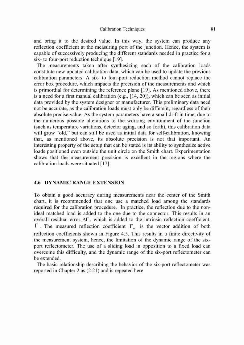
Calibration Techniques 81
and bring it to the desired value. In this way, the system can produce any
reflection coefficient at the measuring port of the junction. Hence, the system is
capable of successively producing the different standards needed in practice for a
six- to four-port reduction technique [19].
The measurements taken after synthesizing each of the calibration loads
constitute new updated calibration data, which can be used to update the previous
calibration parameters. A six- to four-port reduction method cannot replace the
error box procedure, which impacts the precision of the measurements and which
is primordial for determining the reference plane [19]. As mentioned above, there
is a need for a first manual calibration (e.g., [14, 20]), which can be seen as initial
data provided by the system designer or manufacturer. This preliminary data need
not be accurate, as the calibration loads must only be different, regardless of their
absolute precise value. As the system parameters have a small drift in time, due to
the numerous possible alterations to the working environment of the junction
(such as temperature variations, detector aging, and so forth), this calibration data
will grow “old,” but can still be used as initial data for self-calibration, knowing
that, as mentioned above, its absolute precision is not that important. An
interesting property of the setup that can be stated is its ability to synthesize active
loads positioned even outside the unit circle on the Smith chart. Experimentation
shows that the measurement precision is excellent in the regions where the
calibration loads were situated [17].
4.6 DYNAMIC RANGE EXTENSION
To obtain a good accuracy during measurements near the center of the Smith
chart, it is recommended that one use a matched load among the standards
required for the calibration procedure. In practice, the reflection due to the non-
ideal matched load is added to the one due to the connector. This results in an
overall residual error, ∆Γ , which is added to the intrinsic reflection coefficient,
Γ . The measured reflection coefficient mΓ is the vector addition of both
reflection coefficients shown in Figure 4.5. This results in a finite directivity of
the measurement system, hence, the limitation of the dynamic range of the six-
port reflectometer. The use of a sliding load in opposition to a fixed load can
overcome this difficulty, and the dynamic range of the six-port reflectometer can
be extended.
The basic relationship describing the behavior of the six-port reflectometer was
reported in Chapter 2 as (2.21) and is repeated here

82 The Six-Port Technique with Microwave and Wireless Applications
R(Γ)
I(Γ)
Γm
Γ
∆Γ
∆Γ= Error vector
Figure 4.5 Residual reflection’s error effect on the six-port measurement accuracy.
2 22
2i i iP b q= α Γ − , i = 3, 4, 5, and 6 (4.44)
It can be easily shown that the power reading iP corresponding to a device under
test having an impedance near the center of the Smith chart ( )0Γ ≈ can be
approximated with a good accuracy as follows:
( )cos
ii i oi qP P P Γ′≅ − θ − θ (4.45)
where
2 22
2i i iP b q′= α (4.46a)
22
22oi i iP b q= α Γ (4.46b)
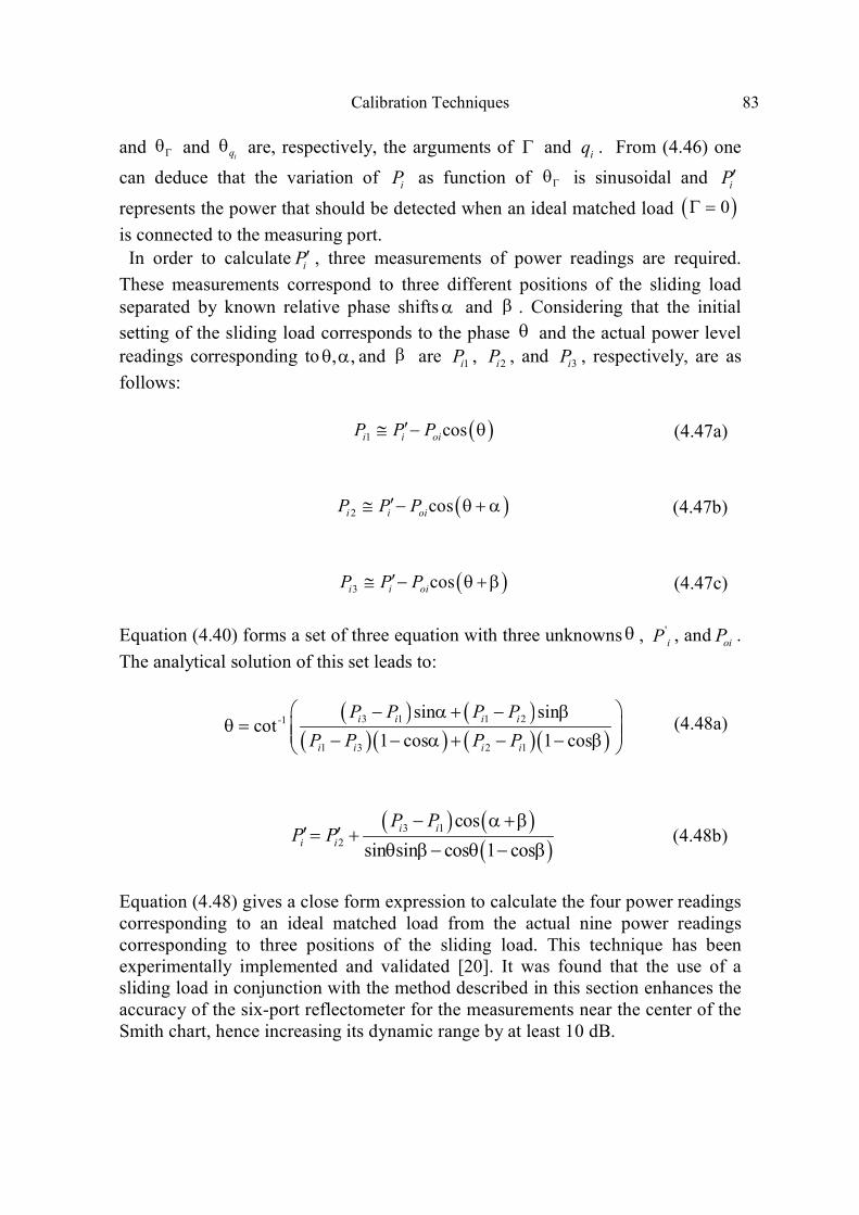
Calibration Techniques 83
and Γθ and iqθ are, respectively, the arguments of Γ and iq . From (4.46) one
can deduce that the variation of iP as function of Γθ is sinusoidal and iP′
represents the power that should be detected when an ideal matched load ( )0Γ =
is connected to the measuring port.
In order to calculate iP′ , three measurements of power readings are required.
These measurements correspond to three different positions of the sliding load
separated by known relative phase shifts α and β . Considering that the initial
setting of the sliding load corresponds to the phase θ and the actual power level
readings corresponding to , ,θ α and β are 1iP ,
2iP , and 3iP , respectively, are as
follows:
( )1 cosi i oiP P P′≅ − θ (4.47a)
( )2 cosi i oiP P P′≅ − θ + α (4.47b)
( )3 cosi i oiP P P′≅ − θ + β (4.47c)
Equation (4.40) forms a set of three equation with three unknowns θ , '
iP , and oiP .
The analytical solution of this set leads to:
( ) ( )( )( ) ( )( )
3 1 1 2-1
1 3 2 1
sin sincot
1 cos 1 cos
i i i i
i i i i
P P P P
P P P P
− α + − βθ = − − α + − − β
(4.48a)
( ) ( )( )
3 1
2
cos
sin sin cos 1 cos
i ii i
P PP P
− α + β′ ′= +
θ β − θ − β (4.48b)
Equation (4.48) gives a close form expression to calculate the four power readings
corresponding to an ideal matched load from the actual nine power readings
corresponding to three positions of the sliding load. This technique has been
experimentally implemented and validated [20]. It was found that the use of a
sliding load in conjunction with the method described in this section enhances the
accuracy of the six-port reflectometer for the measurements near the center of the
Smith chart, hence increasing its dynamic range by at least 10 dB.
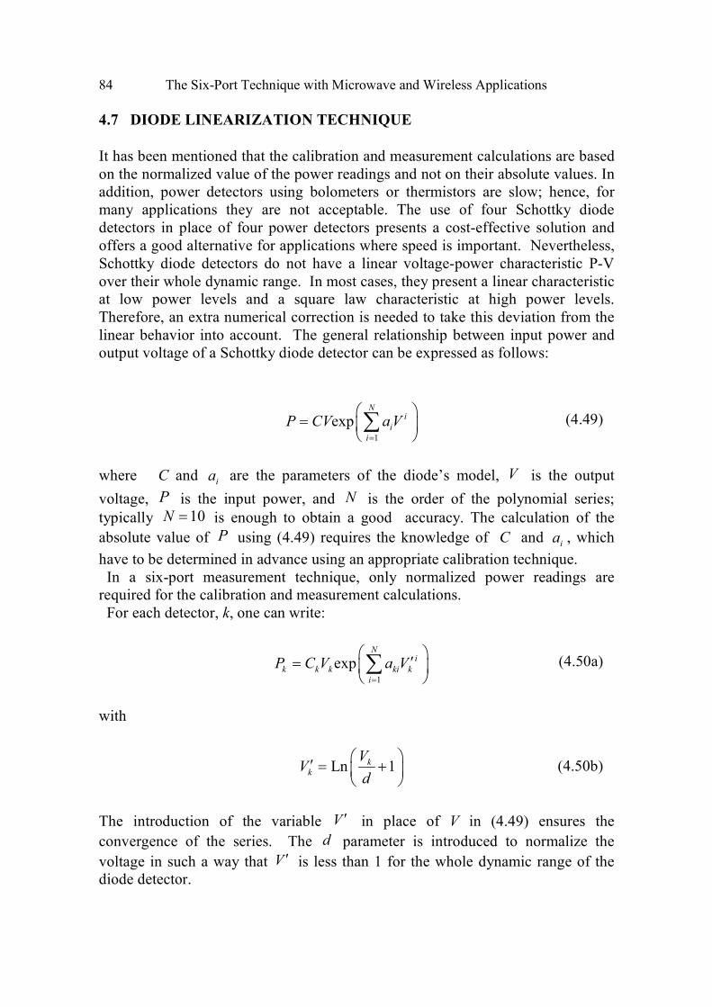
84 The Six-Port Technique with Microwave and Wireless Applications
4.7 DIODE LINEARIZATION TECHNIQUE
It has been mentioned that the calibration and measurement calculations are based
on the normalized value of the power readings and not on their absolute values. In
addition, power detectors using bolometers or thermistors are slow; hence, for
many applications they are not acceptable. The use of four Schottky diode
detectors in place of four power detectors presents a cost-effective solution and
offers a good alternative for applications where speed is important. Nevertheless,
Schottky diode detectors do not have a linear voltage-power characteristic P-V
over their whole dynamic range. In most cases, they present a linear characteristic
at low power levels and a square law characteristic at high power levels.
Therefore, an extra numerical correction is needed to take this deviation from the
linear behavior into account. The general relationship between input power and
output voltage of a Schottky diode detector can be expressed as follows:
1
expN
ii
i
P CV a V=
=
∑ (4.49)
where C and ia are the parameters of the diode’s model, V is the output
voltage, P is the input power, and N is the order of the polynomial series;
typically 10N = is enough to obtain a good accuracy. The calculation of the
absolute value of P using (4.49) requires the knowledge of C and ia , which
have to be determined in advance using an appropriate calibration technique.
In a six-port measurement technique, only normalized power readings are
required for the calibration and measurement calculations.
For each detector, k, one can write:
1
expN
ik k k ki k
i
P C V a V=
′=
∑ (4.50a)
with
Ln 1kk
VV
d
′ = +
(4.50b)
The introduction of the variable V ′ in place of V in (4.49) ensures the
convergence of the series. The d parameter is introduced to normalize the
voltage in such a way that V ′ is less than 1 for the whole dynamic range of the
diode detector.

Calibration Techniques 85
The linearization technique is based on the fact that the six-port junction is a
passive and linear junction; therefore, for a given load, the power reading ratio
3k kp P P= is independent of the power level.
By connecting a passive load at the measuring port and sweeping the power level
of the source, for two different power levels of the generator, j and j+1, one can
write:
, 1 , 1
, 1 1
,
, ,
1
exp
exp
Ni
k k j ki k jk j i
Nik j
k k j ki k ji
C V a VP
PC V a V
+ ++ =
=
′
=
′
∑
∑ (4.51)
Consequently, the normalized power readings are constant, , , 1k j k jp p += , and are
not functions of the power level; thus, one can write
, , , 1 , 1
1 1
3 3, 3 3, 3 3, 1 3 3, 1
1 1
exp exp
exp exp
N Ni i
k k j ki k j k k j ki k ji i
N Ni i
j i j j i ji i
C V a V C V a V
C V a V C V a V
+ += =
+ += =
′ ′
=
′ ′
∑ ∑
∑ ∑ (4.52)
After simplifying and evaluating the logarithm of the right-hand and the left-hand
sides of (4.52), we obtain:
( )( ) ( )( ) , 1 3,
, , 1 3 3, 3, 1
1 3, 1 ,
LnN
k j ji i i iki k j k j i j j
i j k j
V Va V V a V V
V V+
+ += +
′ ′ ′ ′− − − =
∑ (4.53)
Equation (4.53) is a linear one for the unknowns kia and3ia . By using a different
load and different power level, one can form a set of linear equations to be able to
solve for the parameters ( )3,ki ia a . It is important to notice that three different
sets of parameters a3i have to be calculated. Each set is associated with one
pair of power detectors ( )4 3,D D , ( )5 3,D D , and ( )6 3,D D . In practice, three
different loads, (open, short, and matched load) and a power step of 1 dB are
sufficient to obtain accurate solutions for the linear system (4.53), which offers a
reasonable precision in the measurements.

86 The Six-Port Technique with Microwave and Wireless Applications
Once all three sets of coefficient ( )3,ki ia a are obtained, one can calculate the
following power ratio:
1
3
3 3
1
exp
exp
Ni
k ki ki k
kNi
i ki
V a VP
PV a V
=
=
′
= υ
′
∑
∑ (4.54)
where 3
k
k
C
Cυ = and kυ is a real parameter that can be embedded in the five
calibration parameters.
The normalized power readings, kp′ , required to calibrate the six-port
reflectometer, to perform error box calculation, and to calculate the complex
reflection coefficient can be calculated using only voltage measurements as
follows:
( )3 3
1
expN
ik k ki i k
i
p V V a a V=
′ ′= −
∑ (4.55)
The advantages of the technique described above are: (1) no power meter is
needed for the linearization technique, and (2) no precise variable attenuator is
required during the linearization procedure.
In addition, in case the four diode detectors are quasi-identical, there would be
no need for any further corrections to be taken into account for the effect of the
environment temperature or operating frequency.
It is also worth mentioning that the computation effort needed for the
linearization and the measurement procedures is relatively insignificant.
4.8 POWER CALIBRATION TECHNIQUE
It was shown that the six-port reflectometer can be used to calculate the power
flow propagating toward the device under test (DUT). A power calibration,
which calculates an extra real parameter, 2
3α , is needed for that purpose. In the
case of a six-port reflectometer fitted with four diode detectors, the power
calibration calculation is different.
Using (2.39), the absorbed power by any load can be calculated as follows:

Calibration Techniques 87
( ) ( )2 22 2
3 3 33
1
2 22 2
3 3
1 exp1
1 1
Ni
L i kL i
L
c C V a Vc PP
c c
=
′− Γ − Γ
= =α Γ + α Γ +
∑ (4.56)
The only unknown quantities are the ratio 2
3 3C α and the coefficients3ia . It is
assumed herein that c is the parameter of the error box.
It was mentioned above that the six-port junction is a linear one. Therefore, for a
fixed load connected to the measuring port, the ratio of the power absorbed by the
load for two different levels of the generator is the same as the ratio of the third
power readings corresponding to these power levels of the generator. Therefore,
one can deduce:
3 3, 1 3 3, 111
3 3, 3 3,
1
exp
exp
Ni
j i jjiL
j NiL
j i ji
C V a VP
PC V a V
+ ++=
=
′
=
′
∑
∑ (4.57)
By connecting an absolute power meter to the measuring port and after
simplifying and evaluating the logarithm of the right-hand and the left-hand sides
of (4.57), one can deduce the following equation
( )( ) , 3, 1
3 3, 3, 1
1 , 1 3,
LnN
PM j ji ii j j
i PM j j
P Va V V
P V+
+= +
′ ′− =
∑ (4.58)
where ,PM jP and
, 1PM jP + are the two power readings given by the power meter.
By sweeping the power level of the source, one can generate a set of equations,
similar to (4.58), which can be grouped to form a linear system. The solution of
this linear system gives the coefficients 3ia needed to calculate the power
absorbed by the load in (4.56). Once these coefficients are obtained, for a given
power level, i, of the source, one can write
( )
2 2
,3
22 23
3, 3
1
1
1 exp
PM i PM
Ni
PM i i ki
P c cC
c V a V=
Γ +=
α ′− Γ
∑
(4.59)
where the remaining unknown ratio 2
3 3C α can be calculated.

88 The Six-Port Technique with Microwave and Wireless Applications
References
[1] Ghannouchi, F. M., and R. G. Bosisio, “An Alternative Explicit Six-Port Matrix Calibration Formalism Using Five Standards,” IEEE Trans. Microwave Theory Tech., Vol. 36, No. 3, pp.
494–498, March 1988.
[2] Engen, G. F., “Calibrating the Six-Port Reflectometer by Means of Sliding Terminations,” IEEE Trans. Microwave Theory Tech., Vol. MTT-26, pp. 951–957, 1978.
[3] Susman, L., “Calibration of Six-Port Reflectometer Using Projection Geometry Concept,”
Electronic Letters, Vol. 20, No. 1, pp. 9–11, 1984.
[4] Somlo, P. I., and J. D. Hunter, “A Six-Port Reflectometer and Its Complete Characterization by
Convenient Calibration Procedures,” IEEE Trans. Microwave Theory Tech., Vol. MTT-30, No.
2, pp. 186–192, February 1982.
[5] Hunter, J. D., and P. I. Somlo, “An Explicit Six-Port Calibration Method Using Five Standards,”
IEEE Trans. Microwave Theory Tech., Vol. MTT-33, No. 1, pp.69–71, January 1985.
[6] Qian, C. Z., “An Improved Method for Six-Port Reflectometer Calibration,” IEEE Trans. Instr. & Meas., Vol. IM-34, No. 4, pp. 611–615, December1985.
[7] Ghannouchi, F. M., and R. G. Bosisio, “Calibration and Measurement of Six-Port Reflectometer
Using a Matrix Approach,” Technical Report EPM-86/48, Ecole Polytechnique of Montreal, October 1986.
[8] Engen, G. F., “An Improved Circuit for Implementing the Six-Port Technique of Microwave
Measurements,” IEEE Trans. Microwave Theory Tech., Vol. MTT-25, No. 12, pp. 1080–1083, December 1977.
[9] Ghannouchi, F. M., and R. G. Bosisio, “Calibration and Measurement of Six-Port Reflectometer
Using a Matrix Approach,” Technical Report EPM/RT-86/46, Report EPM/RT-86/47 and Report EPM/RT-86/48, Ecole Polytechnique of Montreal, October 1986.
[10] Hoer, C. A., “Choosing Line Lengths for Calibrating Network Analyzers,” IEEE Trans. Microwave Theory Tech., Vol. 31, pp. 76–77, January 1983.
[11] Ghannouchi, F. M., and R. G. Bosisio, “An Improved Load Formulation for Use in Six-Port
Calibration Methods,” Alta Frequenza, Vol. 57, No. 8, pp. 497–499, 1988.
[12] Engen, G. F., “A Least Square Solution for Use in the Six-Port Measurement Technique,” IEEE Trans. Microwave Theory Tech., Vol. MTT-28, pp. 1473–1477, December 1980.
[13] Riblet, G. P., and E. R. B. Hansson, “Aspects of the Calibration of a Single Six-Port Using a
Load and Offset Reflection Standards,” IEEE Trans. Microwave Theory Tech., Vol. MTT-30, pp. 2120–2125, 1982.
[14] Ghannouchi, F. M., and R. G. Bosisio, “The Six Port Reflectometer and Its Complete Calibration
by Four Standard Terminations,” IEE Proceedings-H: Microwaves, Antennas and Propagation, Vol. 135, No. 4, pp. 285–288, August 1988.
[15] Hodgetts, T. E., and E. J. Griffin, “An Unified Treatment of the Theory of Six-Port
Reflectometer Calibration Using The Minimum of Standards,” Royal Signals and Radar Establishment, UK, Report 83003, 1983.
[16] Potter, C. M., and G. Hjipieris, “A Robust Six- to Four Reduction Algorithm,” IEEE MTT Symposium Proceedings , Vol. 3, pp. 1263–1266, 1993.

Calibration Techniques 89
[17] Yakabe, T., F. M. Ghannouchi, E. E. Eid, K.Fujii, and H. Yabe, “Six-Port Self-Calibration
Based on Active Loads Synthesis,” IEEE Trans. Microwave Theory Tech., Vol. 50, No. 4, pp. 1237–1239, April 2002.
[18] Ghannouchi, F. M., and R. G. Bosisio, “A Wide Band Millimeter Wave Six-Port Reflectometer
Using Four Diode Detectors Calibrated Without Power Ratio Standard,” IEEE Trans. Instrumentation and Measurement,. Vol. 40, pp. 1043–1046, Decemeber 1991.
[19] Le, D. L., and F. M. Ghannouchi, “Source–Pull Measurements Using Reverse Six-Port
Reflectometers with Application to MESFET Mixer Design,” IEEE Trans. Microwave Theory Tech., Vol. 42, pp. 1589–1595, September. 1994.
[20] Yakabe, T., M. Kinoshita, and H. Yabe, “Complete Calibration of a Six-Port Reflectometer with
One Sliding Load and One Short,” IEEE Trans. Microwave Theory Tech., Vol. 42, pp. 2035–2039, November 1994.


91
Chapter 5
Six-Port Network Analyzers
In the previous chapters, the fundamentals, the calibration techniques, and the
design of six-port reflectometers have been presented and discussed. This chapter
presents the theory and discusses the design and the calibration of six-port based
network analyzer. The theory and the calibration of a two-port six-port vector
network analyzer are presented. A six-port based de-embedding technique needed
for the measurement of devices without coaxial terminals is also presented. The
theory, the measurement, and the calibration of a tri-six-port-based network
analyzer are presented. An N-six-port measurement technique, which requires
only a one-step connection, is also presented and discussed. Finally, a single six-
port junction based N-port vector network analyzer is presented in which the six-
port junction is used as a complex wave comparator.
5.1 GENERAL FORMULATION
It was shown in Chapter 1 that the six-port reflectometer is capable of making
simultaneous power flow and impedance measurements using only amplitude
measurements while no phase measurements are required. The use of two six-port
reflectometers in conjunction with an appropriate calibration procedure can lead to
the determination of the four scattering parameters of any two-port device under
test (DUT) [1-4]. The general block diagram of a two-port six-port based network
analyzer is shown in Figure 5.1.
CNT1 and CNT2 are two repeatable phase and amplitude controllers inserted in
branch 1 and branch 2 of the six-port network analyzer (SPNA). CNT1 and CNT2
are used to vary the amplitude and the phase of the emerging signal a1 and a2
from the two measuring ports of the two six-port junctions, SP1 and SP2.
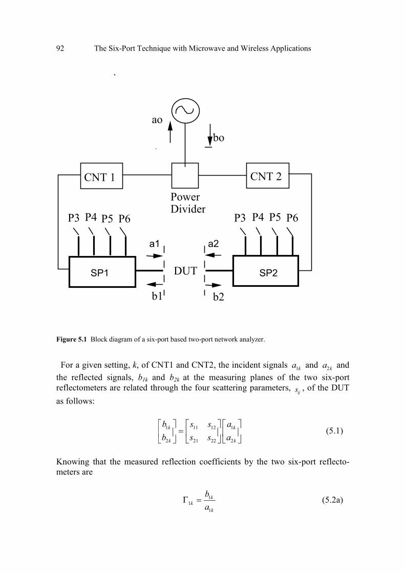
92 The Six-Port Technique with Microwave and Wireless Applications
Figure 5.1 Block diagram of a six-port based two-port network analyzer.
For a given setting, k, of CNT1 and CNT2, the incident signals 1ka and
2ka and
the reflected signals, b1k and b2k at the measuring planes of the two six-port
reflectometers are related through the four scattering parameters, sij
, of the DUT
as follows:
1 111 12
2 221 22
k k
k k
b as s
b as s
=
(5.1)
Knowing that the measured reflection coefficients by the two six-port reflecto-
meters are
1
1
1
kk
k
b
aΓ = (5.2a)
CNT 1 CNT 2
Power Divider
P3 P4 P5 P6 P3 P4 P5 P6
DUT
b1 b2
ao
bo
a1 a2
SP2SP1

Six-Port Network Analyzers 93
2
2
2
kk
k
b
aΓ = (5.2b)
one can rewrite (5.1) in the following format
1 11 12k ks s gΓ − = (5.3a)
2 22 21k ks s gΓ − = (5.3b)
where 2
1
kk
k
ag
a= . The use of two different settings for the amplitude and phase
controllers, k=1, and 2, leads to obtaining a set of four linear equations similar to
(5.3). The solution of this set gives the four unknown ijs parameters.
5.2 CASE OF A RECIPROCAL TWO-PORT DUT
The multiplication of (5.3a) by (5.3b) allows the elimination of kg and gives the
following equation:
11 2 22 1 1 2k k k ks sΓ + Γ − ∆ = Γ Γ (5.4)
where 11 22 12 21s s s s∆ = − . Equation (5.4) can be used to calculate the S parameters
of a reciprocal two-port DUT s12 = s21( ). In such a case three excitations, k =1, 2,
and 3, are required to form a set of three complex linear equations with three
unknowns 11s ,
22s , and ∆ . The solution of this linear system leads to a complete
knowledge of 11s and
22s and to a partial knowledge of 21s .
21 11 22s s s= −∆ (5.5a)
( ) ( )21 11 22arg args s s n= −∆ + π (5.5b)

94 The Six-Port Technique with Microwave and Wireless Applications
with n =1, 2, ..., N. The nonambiguous determination of the phase of s21 requires
multifrequency measurements or the knowledge of an approximate value for the
phase of s21 .
It is important to notice that in cases of a reciprocal DUT, no extra calibration,
besides the calibration of each six-port reflectometer for reflection measurements,
is required to determine the S parameters of the two-port device under test.
5.3 CASE OF AN ARBITRARY TWO-PORT DUT
In the case of an arbitrary DUT, (5.3) can be rewritten as follows:
111 12
221 22
1 k
k k k
s s
g gs s
Γ = Γ
(5.6)
Equation (5.6) shows that the measurements of 1kΓ and
2kΓ , at two different
excitations, k =1 and 2, are sufficient to determine the four S parameters of any
DUT provided that kg is known for these two excitations. The determination of S
parameters is based on the solution of a set of four complex linear equations with
four unknowns. At this stage, kg is still unknown and has to be calculated using
the calibration parameters of the SPNA which should be obtained in advance
using the procedure explained next.
The determination of the excitation kg , when the DUT is connected to the
SPNA and when the branch controllers are set at condition k, is based on the
characterization of the calibration of three-port network resulting from the two
measuring planes, 1 and 2, and the reference plane at the output of the RF signal
generator, plane 0, as shown in Figure 5.2.
The relationships between the incident ikb and the reflected ika waves at the two
measuring planes 1 and 2 are:
1 10 0 11 1 12 2
k k kk k k ka u b u b u b= + + (5.7a)
2 20 0 21 1 22 2
k k kk k k ka u b u b u b= + + (5.7b)

Six-Port Network Analyzers 95
Figure 5.2 The three-port network needs to be characterized at both controller settings.
where u ijk
represent the scattering parameters of the three-port network at
excitation k. Equation (5.7) can be rewritten in matrix format as follows:
111 1 12 2 10
0
221 1 22 2 20
1
1
k k kkk k
kk k kkk k
au u ub
au u u
− Γ − Γ= − Γ − Γ
(5.8)
Using Crammer’s rules and after algebraic manipulations, one can obtain:
( ) ( )
( )1
21
k k k k kk
k k k
B A D Ag
C A
+ Γ=
+ Γ (5.9)
where
10 ,kkA u=
20 ,kkB u=
20 12 10 22
k k k kkC u u u u= −
and
10 21 20 11
k k k kkD u u u u= −
source
three-port
calibration
networks
k=1 and 2
a1k
a2k
b2kb1k
b0k a0k
two-port
DUT
plane 0
planes 1 and 2
96 The Six-Port Technique with Microwave and Wireless Applications
The calculation of gk needed for the determination of the DUT’s S parameters is
straightforward using the measured reflection coefficients Г1k , and Г2k, when the
DUT is connected to the measuring planes, and the calibration parameters of the
SPNA k kB A , k kC A , and k kD A . The determination of these parameters is
based on the following equation obtained by substituting (5.9) into (5.3a) and by
replacing 2
1
kk
k
ag
a= by its equivalent expression deduced using (5.3a), and which
is equal to ( )1 11 12k s sΓ − :
( )12 22 1 12 1 1 11
s s s s s s s sk k kk k k
k k k
B C Ds s s s
A A A+ ∆ − Γ + Γ = Γ − (5.10)
with s= 1, 2, and 3 and k= 1 and 2, and sijs are the scattering parameters of the
standards. The use of the same three known and different two-port standards (s=1,
2, and 3) for both excitations (k=1 and 2) provides two sets of linear equations,
one set per excitation. Each set includes three equations and three unknowns
( ,k kB A k kC A , k kD A ). The solution of these sets allows the calculation of the
six calibration parameters, three per excitation.
Alternatively, it is possible to use three unknown reciprocal two-port standards
and three different excitations in place of two known two-port standards and two
excitations to solve for the six calibration parameters. The procedure to determine
the S parameters of a reciprocal two-port standard, described in Section 5.2, can
be applied to calculate the S parameters of the three standards before solving the
linear system (5.10) for k kB A , ,k kC A and k kD A . The calibration technique is
general in the sense that no assumption is made regarding the isolation between
branches and it is applicable whenever the bandwidth of the hardware is
appropriate: six-port junctions, controllers, and so forth.
5.4 SIX-PORT BASED DE-EMBEDDING TECHNIQUE: THEORY
S-parameter measurements of devices whose terminals are noncoaxial (e.g.,
microstrip lines, coplanar waveguide lines, rectangular or circular waveguides,
and fin lines) require the use of a test fixture with suitable transitions between the
DUT terminals and the coaxial terminals of the measurement system [6]. Several
de-embedding techniques have been used to extract the de-embedded (intrinsic) S
parameters of the noncoaxial DUT from the embedded (raw) S′ parameters
obtained using a network analyzer for the DUT mounted in an appropriate test
fixture [7–11]. Based on the above methods, a six-port based technique that
requires three reciprocal unknown two-port standards, a through connection, a

Six-Port Network Analyzers 97
matched two-port standard, and an unmatched two-port standard, is presented in
this section.
The relationship between the scattering parameter matrix entries and the
transmission parameters matrix entries of an arbitrary two-port device is the
following:
11 12 22 11 21 12 11
21 22 2212
1
1
d d s s s s s
d d ss
′ ′ ′ ′ ′− + = = ′′ −
D (5.11)
Figure 5.3 shows a typical setup for S parameters de-embedding purposes. Let A
and B be the transmission matrices associated to the left and right parts of the test
fixture, respectively, and D be the DUT transmission matrix. The incident signals
at the DUT (test fixture) reference planes are aA and aB ( ′ a A , ′ a B ), respectively,
and the reflected signals at the DUT (test fixture) reference planes are bA and bB
( ′ b A , ′ b B ), respectively, as shown in Figure 5.3. A, D, and B are related to the
incident and reflected signals as follows:
A A
A A
b b
a a
′ = ′
A (5.12a)
A B
A B
b b
a a
=
D (5.12b)
B B
B B
b b
a a
′ = ′
B (5.12c)
Using (5.12), one can write
A B B
A B B
b b b
a a a−
′ ′ ′ = = ′ ′ ′
1ADB M (5.13)
M represents the transmission matrix of the test fixture holding the DUT.

98 The Six-Port Technique with Microwave and Wireless Applications
Figure 5.3 General representation of the de-embedding problem.
The two embedded reflection coefficients wA and wB can be measured by the
two reflectometers SPA and SPB for two different excitations, k = 1, and 2. These
excitations are obtained by changing the setting of the amplitude and phase
controllers CNT1 and CNT2, shown in Figure 5.1. This leads to a system of
equations (similar to (5.6)), including four linear equations with four unknowns,
which are the embedded scattering parameters of the test fixture holding the
DUT ′ s 11 , ′ s 12 , ′ s 21 , and ′ s 22 :
11 12
21 22
1 Ak
k k Bk
ws s
g g ws s
′ ′ = ′ ′′ ′
, k =1 and 2 (5.14)
where AkAk
Ak
bw
a
′=
′, and Bk
Bk
Bk
bw
a
′=
′ are, respectively, the embedded reflection
coefficients measured by the two reflectometers SPA and SPB, respectively, and
Bkk
Ak
ag
a
′′ =
′ are the two excitation parameters that should be calculated using the
APC

Six-Port Network Analyzers 99
calibration technique described in section 5.9. The same three reciprocal two-port
standards, which will be introduced in the next section, can be used to calculate
the calibration parameters k kB A′ ′ , k kC A′ ′ , and k kD A′ ′ of the three-port
calibration network needed for the calculation of ′ g k .
The solution of (5.14) leads to the determination of S′ parameters of the test
fixture holding the DUT.
To be able to recover the de-embedded S parameters of the DUT from the
embedded S′ parameters and transmission matrices A and B, which model,
respectively, the right and the left sides of the test fixture delimited by the actual
measuring planes of SPA and SPB, the reference planes of the device under test
(see Figure 5.3) have to be determined in advance. This step constitutes the
calibration procedure which has to be carried out before measuring any DUT.
5.5 TWO-PORT DE-EMBEDDING TECHNIQUE
As mentioned above, the calibration procedure consists of using three unknown
reciprocal two-port standards needed to calculate the entries of the A and B
transmission matrices:
1. A through connection standard:
0 1
1 0
=
1
S (5.15a)
2. A matched reciprocal two-port standard:
0
0
f
f
=
2
S (5.15b)
3. An unmatched reciprocal two-port standard:
g h
h g
=
3
S (5.15c)
Notice that the determinants of the transmission matrices 1D , 2
D , and 3D
corresponding to these standards are equal to unity.

100 The Six-Port Technique with Microwave and Wireless Applications
After placing the three standards successively in the test fixture and measuring
their corresponding embedded reflection coefficients for two different excitations
and applying (5.14) to calculate their corresponding S′ parameters, one can
construct three different transmission matrices, one for each standard, 1M ,
2M
and 3M using the standard transformation between scattering parameters and
transmission parameters shown here:
22 11 21 12 11
2212
1M
1
s s s s s
ss
′ ′ ′ ′ ′− + = ′′ −
(5.16)
A second way to calculate the M matrix is based on the following: from (5.16),
one can see that the knowledge of 11s′ , 22s′ , and ′∆ ( 11 22 12 21s s s s′ ′ ′ ′ ′∆ = − ) leads to
the partial knowledge of the matrix M. Only a normalizing parameter 12s′
corresponding to each standard is still an unknown. These normalizing
parameters can be embedded, respectively, in the matrices 2D ,
3D and T defined
below. In such a case the entries of the nonnormalized transmission matrix M can
be found directly from the solution of a set of linear systems obtained for three
different excitations when the standard, or the DUT, is connected to the measuring
ports as follows:
11 22Bk Ak Ak Bks w s w w w′ ′ ′+ − ∆ = , k= 1, 2, and 3 (5.17)
Let P, Q , R, and T be:
− =1
2 1M M P (5.18a)
− =1
3 1M M Q (5.18b)
− =1
3 2M M R (5.18c)
− =1
3 2D D T (5.18d)
where 2
D and 3
D are the corresponding transmission matrices of the second and
the third standards, respectively.

Six-Port Network Analyzers 101
By using the three equations obtained by means of (5.13), for the three standards,
in conjunction with (5.16), one can derive the following equations:
=2
AD PA (5.19a)
=3
AD QA (5.19b)
=AT RA (5.19c)
Each of the three matrix equations includes a pairs of similar matrices, (D2, P),
(D3, Q), and (R, T), which have been shown mathematically to have the same
trace, determinant, and sign values. The trace invariance property for such
matrices yields the following equation:
ii iiu vΣ = Σ (5.20)
where iiu and iiv are the diagonal entries of a pair of similar matrices ( U , V ).
Applying that property to (5.19a) to calculate the 21s′ parameter of the matched
standard, it is found that two values for f can satisfy the trace invariance property;
( ) ( )2
11 22 11 22
1
4
2
p p p pf
+ + + −= (5.21a)
( ) ( )2
11 22 11 22
2
4
2
p p p pf
+ − + −= (5.21b)
where pij are the entries of matrix P. One way to resolve this ambiguity is to utilize
the fact that, in practice, the entries of the transmission matrix A for an
appropriate test fixture should satisfy the following equation:
12 11
22 21
a a
a a≤ (5.22)
This inequality is equivalent to:
2212
11 211
i
i
f pp
f p p
−≤
−, i = 1 and 2 (5.23)

102 The Six-Port Technique with Microwave and Wireless Applications
Using (5.19b) and (5.19c), and after some algebraic manipulations, one can
calculate the remaining unknown parameters of the third standard as follows:
( ) ( )
2
11 22 11 22
1 fh
q q f r r
−=
+ − + (5.24)
where iiq and iir are the entries of matrices Q and R, respectively.
For the 11s parameter of the unmatched standard, two values for g can satisfy the
trace invariance property:
( )( )1
2 2 21 11 22g fh r r f h= − + + + (5.25a)
( )( )1
2 2 22 11 22g fh r r f h= − − + + + (5.25b)
Again, the sign ambiguity can be resolved knowing that, in practice, the measured
value of 11s , of the third standard, should be comparable to the value of g, in
amplitude and in phase. Therefore, one can use the following criterion to select g:
11 11i is g s g− ≤ + , i= 1 and 2 (5.26)
We assume that the impedances of both the test-ports of SPA and SPB are equal
to the line characteristic impedance, which is 50Ω in practice.
5.6 CALCULATION OF THE ERROR-BOX PARAMETERS
Knowing the parameters of all standards used, we are able now to determine the
aij entries of matrix A by means of (5.18). Each matrix equation can be written as
a set of four homogenous linear complex equations with four unknowns.
Assembling these four sets into one leads to an overdetermined homogenous
complex linear system with four unknowns, aij, and 12 equations:
0=CA (5.27)
where [ ]11 12 21 22
Ta a a a=A and C is a known (12×4) complex matrix.

Six-Port Network Analyzers 103
A singular value decomposition (SVD) technique can be used to solve the above
system to insure a reliable and good solution even if the matrix C presents a bad
condition number. The transmission matrix B, which models the right-hand side
of the test fixture, can easily be calculated using A and M as follows:
B=M-1
A (5.28)
5.7 DETERMINATION OF S PARAMETERS OF AN ARBITRARY DUT
To be able to calculate the S parameters of any DUT, we first need to determine
the S′ matrix of the test fixture holding the DUT using (5.14). This procedure
requires the use of good quality phase and amplitude controllers CNT1 and CNT2
with reliable repeatability.
Using the transmission matrices of the two error box networks A and B, the
transmission matrix of the DUT can be obtained using the following equation:
−= 1D A MB (5.29)
where M is the transmission matrix of the test fixture holding the DUT and is
related to its S′ parameters via (5.14).
The standard transformation between the transmission parameter matrix and the
scattering parameter matrix allows the calculation of the de-embedded S
parameters of the DUT as follows:
12
11
22
ds
d= (5.30a)
12 21
12 11
22
d ds d
d
= −
(5.30b)
21
22
1s
d= (5.30c)
and
21
22
22
ds
d= − (5.30d)
The above calibration and de-embedding procedures can be implemented on a
network analyzer comprising two reflectometers (e.g., six-port network
analyzers), or can also be implemented on four CNAs that directly provide the
embedded S′ parameters. In this case, the four measurement matrices M1, M2,
M3, and M can be directly calculated using (5.16). When a four-channel network

104 The Six-Port Technique with Microwave and Wireless Applications
analyzer is used, only excitation 1 and excitation 2 are needed to compute the S
parameters of an arbitrary DUT.
In the case of a purely reflecting DUT ( )12 21 0s s′ ′= = , the transformation between
the scattering matrix, S, and the transmission matrix D becomes singular, as can
be deduced from (5.28). Therefore, a test to detect such a situation is required and
an alternative method for calculating 11s and 22s should be included in the
algorithm. A test may consist of checking whether the determinant of M in (5.14)
goes to zero, and in a such a case, the following relationships can be used to
calculate 11s and 22s .
[ ]
1111
22det
A
A
ws
w
− α=
− α + α (5.31a)
and
[ ]
B 1122
22det B
ws
w
− β=
− β + β (5.31b)
where αij and βij are the entries of the scattering matrices ′A and B′ associated
with the error box matrice A and B, which can be easily calculated using the
transmission matrices A and B and the embedded reflection coefficient Aw and
Bw measured when the DUT is connected to one of the measuring reference
planes.
It is important to notice that the through connection standard can be replaced by
a delay line as in the line reflect line (LRL) technique. In this case, the equivalent
reference plane of a virtual through connection positioned at the middle of this
delay line is considered in the computation. The difference between the delay line
and the matched standard electrical length is considered as the electrical length of
the matched standard in the computation.
5.8 TRI-SIX-PORT NETWORK ANALYZER
The block diagram of the three-six-port network analyzer (TSPNA) is shown in
Figure 5.4 [15]. The basic relationship that relates the incident signals to the
reflected signals for a given three-port DUT is
=b Sa (5.32)

Six-Port Network Analyzers 105
Device under
testSP3
CNT
1
CNT
3
SP1
SP
2
CNT
2
power divider
source
plane 1 plane 3
a1k
b1k a3k
b3k
a0k b0kplane 0
a2k b2k
plane2
Figure 5.4 Block diagram of TSPNA.
where ( )1 2 3, ,
Ta a a=a , and ( )1 2 3
, ,T
b b b=b . When the amplitude and phase
controllers, CNT1, CNT2, and CNT3, are set at condition k, (5.32) can be
reexpressed as follows:
k k
′=SG G (5.33)

106 The Six-Port Technique with Microwave and Wireless Applications
where ( )1 2 31 , ,
T
k kk g g=G , ( )1 2 2 3 3, ,T
k k k k kk g g′ = Γ Γ ΓG , 1
ikik
k
ag
a= , and ik
ik
ik
b
aΓ =
with i = 1, 2, and 3; and k = 1, 2, and 3.
Γik is the reflection coefficient measured by SPI, for the excitation k. The three
six-port reflectometers are assumed to be calibrated for reflection measurements.
For the four-port network delimited by the three measuring planes (planes 1, 2,
and 3) and the reference plane at the output of the RF signal generator (plane 0)
shown in Figure 5.4, the following equation can be written:
okb= k
k k 0U a U (5.34a)
where
11 1 12 2 13 3
21 1 22 2 23 3
31 1 32 2 33 3
1
1
1
k k kk k k
k k kk k k
k k kk k k
u u u
u u u
u u u
− Γ − Γ − Γ
= − Γ − Γ − Γ − Γ − Γ − Γ
kU
(5.34b)
and ( )1 2 3, ,
Ta = k k kk a a a and ( )10 20 30, ,k k ku u u=
Tk
0U and okb is the incident signal at
the generator port of the four-port network.
Solving (5.34a) for aik using Crammer’s rules, one can easily write
( )( )
( )( )
( )( )
0
11 1
0
det
b det det
det det
b det
ik
k ik
k k
k
U
U U
U U
U
kikik
k
k
ag
a= = = (5.35)

Six-Port Network Analyzers 107
Figure 5.5 Calibration of the TSPNA.
Here ( )detik
U ( ( )1detk
U ) is the determinant of matrix kU with its ith (first)
column replaced by a column vector k
0U . The assembling of (5.33) obtained for
three different excitations, in one matrix equation gives:
21 31 11
21 31 12
21 31 13
22 32 21
22 32 22
22 32 23
23 33 31
23 33 32
23 33 33
1 0 0 0 0 0 0
0 0 0 1 0 0 0
0 0 0 0 0 0 1
1 0 0 0 0 0 0
0 0 0 1 0 0 0
0 0 0 0 0 0 1
1 0 0 0 0 0 0
0 0 0 1 0 0 0
0 0 0 0 0 0 1
g g s
g g s
g g s
g g s
g g s
g g s
g g s
g g s
g g s
11
21 21
31 31
12
22 22
32 32
13
23 23
33 33
g
g
g
g
g
g
Γ Γ Γ
Γ = Γ
Γ Γ
Γ Γ
(5.36)
source
three-port
calibration
networks
k=1, 2, and 3
aik bik
bjk ajk
bok aokreciprocal
two-port
standards
s=1, 2, and 3 matched
load
step1 i=1, j=2
step2 i=1, j=3
step3 i=2, j=3

108 The Six-Port Technique with Microwave and Wireless Applications
The solution of the linear system (5.36) provides the nine unknown S parameters
of the three-port DUT.
The calculation of the six ikg (i = 1 and 2; k = 1, 2, and 3) is easily obtained
using (5.35). For example, 23g should be calculated as follows:
3 3
11 13 13 33
3 3 3 3
21 13 20 10 23 33
3 3 3 3
31 13 30 10 33 33
23 3 3
12 23 13 33
3 3 3 3
20 10 22 23 23 33
3 3 3 3
30 10 32 23 33 33
1 1
1
1
1
1
u u
u u u u
u u u ug
u u
u u u u
u u u u
− Γ − Γ
− Γ − Γ
− Γ − Γ=
− Γ − Γ
− Γ − Γ
− Γ − Γ
(5.37)
The calibration of the TSPNA can be subdivided into three parts. As shown in
Figure 5.5, each part is equivalent to the calibration of a dual six-port network
analyzer. By connecting a matched load at one port of the four-port network
shown in Figure 5.5, the four-port network will be reduced to a three-port
network, which can be characterized by determining its nine parameters, three for
each excitation, using the method explained in section 5.2. The rotation of this
matched load between the measuring ports of the three reflectometers and the
calculation of the corresponding calibration parameters kiju ,and 0 0
k kj iu u lead to
the complete determination of the 27 calibration parameters, 9 per excitation,
needed for the operation of the TSPNA.
kiju , and 0 0
k kj iu u can be deduced from the calibration parameters of each pair
of six-port reflectometers (SPi, SPj), ( )k k ijB A , ( )k k ij
C A , and ( )k k ijD A as
follows.
( )0
0
kj
k kk iji
uB A
u= (5.38a)
and
( ) ( )
( ) ( )
;
;
kk k k k jjij ij
kij k
k k jj k kij ij
D A B A u i ju
C A u B A j i
+ >
= + >
(5.38b)
with ukjj as the reflection coefficient of the jth port of the four-port network when
all the remaining ports are terminated by matched loads. These parameters can be

Six-Port Network Analyzers 109
easily measured in advance, using a calibrated six-port reflectometer. In
conclusion, three steps are required for the calibration of TSPNA:
Step 1: Calibration of (SP1, SP2), as explained in section 5.2, while SP3 is
terminated by a matched load for each excitation (k = 1, 2, and 3). This step gives
the following nine complex parameters ( )20 10 21 12, ,k k k ku u u u .
Step 2: Calibration of (SP1, SP3), as explained in section 5.2, while SP2 is
terminated by a matched load for each excitation (k = 1, 2, and 3). This step gives
the following nine complex parameters ( )30 10 31 13, ,k k k ku u u u .
Step 3: Calibration of (SP2, SP3), as explained in section 5.2, while SP1 is
terminated by a matched load for each excitation (k = 1, 2, and 3). This step gives
the following nine complex parameters ( )30 20 32 23, ,k k k ku u u u .
The method to determine the 27 calibration parameters required to calculate the
six excitation parameters ikg (i = 2 and 3; k = 1, 2, and 3) is explicit, rigorous, and
does not requires any isolation between branches. Only three unknown reciprocal
two-port standards, three repeatable and absorptive switches, and two repeatable
amplitude and phase controllers are required for the operation of the TSPNA.
5.9 N-SIX-PORT NETWORK ANALYZER
The above described technique for the calibration and measurements of the
TSPNA can be easily extended to handle the N-six-port network analyzer
(NSPNA). The block diagram of the NSPNA is shown in Figure 5.6. The number
of the six-port reflectometers and the number of excitations required should be
equal to the number of ports, N, of the DUT, and the calibration procedure
includes 2
nC steps. Each step is to calibrate each pair of six-port reflectometers
and to deduce the 3N complex parameters ( )0 0 , ,k k k ki j ij jiu u u u , k =1, 2, 3, ..., N. The
calibration procedure of the NSPNA is illustrated in Figure 5.6.
Therefore, the total number of the calibration parameters is 23 nNC and the linear
system to be solved for the calculation should include 2N equations to solve for
the 2N unknown S parameters.
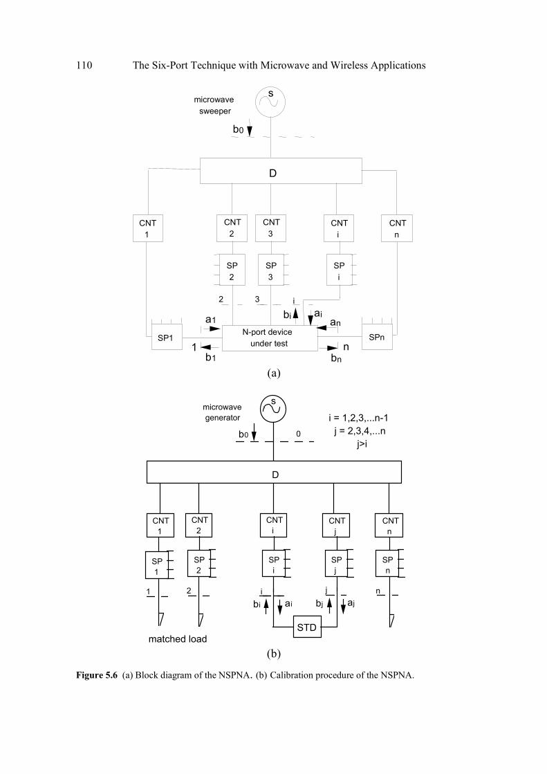
110 The Six-Port Technique with Microwave and Wireless Applications
(a)
CNT
1
CNT
n
STD
SP
i
CNT
i
D
microwave
generator
b0
s
SP
j
CNT
j
CNT
2
SP
2
2 i j
ajbj
0
1
SP
1
SP
n
n
aibi
matched load
i = 1,2,3,...n-1
j = 2,3,4,...n
j>i
(b)
Figure 5.6 (a) Block diagram of the NSPNA. (b) Calibration procedure of the NSPNA.
N-port device
under test
CNT
1
CNT
n
SPnSP1
SP
3
CNT
3
D
microwave
sweeper
a 1
b0
s
b 11 n
bn
an
SP
i
CNT
i
SP
2
CNT
2
2 3 i ai bi

Six-Port Network Analyzers 111
5.10 A SINGLE SIX-PORT N-PORT VECTOR NETWORK ANALYZER
The six-port junction operates as a relative two-channel receiver in this
application [16]. As explained, the six-port can perform reflection coefficient
measurements at the test port while the input port is connected to an RF generator
and the four remaining ports to power/voltage detection sensors. In this
configuration, shown in Figure 5.7, incident and reflected waves ain and aout are
completely independent and the six-port junction reflectometer operates as a wave
comparator providing the ratio aout/ ain. This ratio is a function of the measured
reflection coefficient and the calibration parameters, which have to be determined
in advance, as follows
Figure 5.7 A six-port wave comparator.
( )
1
21
out out
in out
a C
a C
Γ=
− Γ (5.39)
where outout
out
a
bΓ = , C1 and C2 are the calibration parameters characterizing the
two-port network constituted by the six-port junction when the four reading ports
are terminated by the four power/voltage sensors. These parameters have to be
determined in advance, and Γout is the measured reflection coefficient at port 2 of
the six-port junction. According to Chapter 4, when the six-port junction includes
a reference port, the reflection coefficient measurement is independent from the
generator impedance. Using this hypothesis and a very simple flow graph, the

112 The Six-Port Technique with Microwave and Wireless Applications
coefficients 1
C and 2
C can be related directly to the S parameters of six-port
reflectometer as follows:
C1 = S21,SP and C2 = S22,SP (5.40)
2N
PS
T S
witch
Bo
x
Figure 5.8 A six-port automated network analyzer.
Using the six-port as a two-channel receiver and adding an appropriate test set
designed using switches and couplers and power dividers, a single six-port
junction N-port vector network analyzer can be designed. The block diagram of
the proposed system is shown in Figure 5.8.
For calibration and measurement purposes of S parameters, the incidents and/or
the reflected waves ai and bi are sampled via N two-dual directional couplers.
Using the primary SPNT absorptive switch box, the signal generator is routed
successively to the iP ports of the DUT. For a given setting of the latter switch
box, the secondary absorptive 2NPST switch box is used to route all ai and bi to
Six-Port Network Analyzers 113
the measuring port (port 2) of the six-port junction, respectively. The ratio
between the raw air or bir and the reference wave aRef feeding port 1 of the six-
port junction can be provided by the two-channel six-port receiver as follows by
the six-port receiver:
( )
21,
22,
or
1
SPi i
ref SP
sb aR
a S
Γ= =
− Γ (5.41)
with 2
2
b
aΓ = , where Γ is the measured reflection coefficient at the output of six-
port. For full vector calibration and de-embedding purposes needed to transfer the
measurement’s reference planes form the inputs of the six port junction to the
DUT, the technique presented in Section 5.5 or several established techniques
such as QSOLT [9] or TRL [17] can be used as in the case of two-port
commercial VNA. For multiport VNA the calibration algorithm presented in the
next section can be used to de-embed the raw S parameters measured at the SPR
ports to the N-port of the DUT.
5.11 N-PORT CALIBRATION ALGORITHM
In the proposed setup, the measurements are performed at the SPR as ratios
between channel 1 as a receiver for the incident and reflected waves and channel
2 as a reference. This first requires calibration of the six-port junction as a
reflectometer using one of the techniques reported in Chapter 3 [12, 13, 17]. Then
the raw S parameters measured at the SPR ports have to be de-embedded to get
the true S parameters of the DUT [5, 14, 15].
The calibration algorithm used in this measurement setup is based on making
full calibration for port 1 using OSL standards and then making two-port
calibration using a (THRU) standard. The block diagram of the N-port calibration
procedure is shown in Figure 5.9. The calibration steps can be described as
follows.
114 The Six-Port Technique with Microwave and Wireless Applications
Step 1: Performing OSL at port 1
This step is performed to calculate the parameters ( 11 22
1 1,e e , and
11 22 21 12
1 1 1 1 )e e e e e∆ = − of the error box representing the transfer from port 1 to the
six-port receiver (SPR) reference plane as shown in Figure 5.9. These parameters
can be calculated by measuring the reflection coefficients of OSL at port 1 at each
frequency point using (5.33)–(5.36).
The reflection coefficient at the standard connected to port 1 plane (ΓSTD) can be described as a function of the measured reflection coefficient at the SPR plane (Γm) and the error box matrix
1
ije as follows:
12 21 22
11 1 1 1 1
1 22 22
1 11 1
STD STDm
STD STD
e e e ee
e e
Γ −∆ Γ +Γ = + =
− Γ − Γ + (5.42)
Using open, short, and load standards, one can write
(5.43)
The error box Ei models the interconnection between the SPR measurement port
and the port i of the DUT and relates the reflected to the incident waves, defined
according the following equation
(5.44)
111
1
22
1
1 *
1 *
1 *
open Mopen open Mopen
short Mshort short Mshort
load Mload load Mload
e
e
e
− Γ Γ −Γ Γ = Γ Γ −Γ Γ ∆ Γ Γ −Γ Γ
.mi mi
iduti duti
b aE
a b
=

Six-Port Network Analyzers 115
⋮
Figure 5.9 Block diagram of the N-port calibration procedure.
where openΓ , shortΓ , and loadΓ are the actual reflection coefficients of the OSL
standards. ,MopenΓ ,MshortΓ and MloadΓ are the measured reflection coefficients of
the OSL standards using SPR.
Step 2: THRU Connection between port 1 and each port of the N-ports
By performing this step, the parameters of the remaining error boxes between the
N-ports and the SPR can be calculated as functions of the measured S parameters
of the THRU using the following relations:
1 11
22 1
22 1 11
11 1 11 1( )
T NmKK
K T Km
S ee
t e S e
−=
+ − (5.45)
22
11 1 1
22 22
11
T K KKK mKK
K
t ee S
e e= −
− (5.46)
( )2
22 22
11 1
1 1
11
1 KT K T KKK mK m K
e eT S S
t
−= − (5.47)

116 The Six-Port Technique with Microwave and Wireless Applications
( )1 11 11
1 1 11T KK m K KT S e e= − and ( )1 11 11
1 1 11TKK mK KT S e e= − (5.48)
where k is the port number and Sm are the measured S-parameters of the THRU
connected between port 1 and port K. Step 2 will be repeated until K=N where N is the number of ports.
Step 3: Calculation of the term KJT , which characterizes the path between port k
and port j
12 21 1 1
11
K JKJ k j
T TT e e
t= = (5.49)
Step 4:De-embedding of the DUT’s S parameters
After calculating all the parameters of the error boxes, the de-embedded S
parameters of the DUT can be calculated using (5.40).
1
11*( * )S A I A −= + Γ (5.50)
where
( )
( )
( )
11
11 1 1
11 1
11
22 1 221
21 22 2
11
1
1
m m N
N
m m Nm
N
mNN NmN
N NN
S e S
t t
S e SSA t t t
S eS
t t
−
− = −
⋯ ⋯
⋯
⋮ ⋮ ⋮ ⋮
⋯ ⋯
(5.51)
11 11 11 11
11 1 2 3diag( , , , )Ne e e eΓ = … (5.52)
and I is the identity matrix. This calibration algorithm has the advantage of taking
the cross-talk between ports into consideration, which leads to accurate results
compared to other calibration algorithms. It also avoids the problem of

Six-Port Network Analyzers 117
impractical line lengths when using the TRL method at relatively low frequencies.
References
[1] Kaliouby, L., and R. G. Bosisio, “A New Method for Six-Port Swept Frequency Automatic Network Analysis,” IEEE Trans. on Microwave Theory and Tech., Vol. 32, No. 12, pp. 1678–
1682, December 1984.
[2] Cronson, H. M., and L. Susman, “A Six-Port Automatic Network Analyzer,” IEEE Trans. on Microwave Theory and Tech., Vol. MTT-25, pp. 1086–1091, December 1977.
[3] Engen, G. F., and C. A. Hoer, “Thru-Reflect-Line: An Improved Technique for Calibrating the
Dual Six-Port Automatic Network Analyzer,” IEEE Trans. on Microwave Theory and Tech., Vol. MTT-27, pp. 987–992, 1979.
[4] Li, S., and R. G. Bosisio, “A Calibration of Multiport Reflectometer by Means of Four
Open/Short Circuit,” IEEE Trans. on Microwave Theory and Tech., Vol. MTT-30, pp. 1085–1090, July 1982.
[5] Li, S. H., and R. G. Bosisio, “The Automatic Measurement of N-Port Microwave Junction by Means of the Six-Port Technique,” IEEE Trans. Instr. Meas., Vol. IM-31, No. 1, pp. 40–43,
1982.
[6] Maury, M. A., S. L. March, and G. R. Simpson, “TRL Calibration of Vector Automatic Network Analyzers,” Microwave Journal, Vol. 30, No. 5, pp. 387–382, May 1987.
[7] Rubin, D., “De-Embedding MM-Wave MICs with TRL,” Microwave Journal, Vol. 33, No. 6,
pp. 141–150, June 1990.
[8] Locatelli, G. P., “De-Embedding Techniques for Device Characterization,” ALTA FREQ., Vol.
57, No. 5, pp. 267–272, June 1988.
[9] Engen, G.F. and C.A. Hoer, “Thru-Reflect-Line: An Improved Technique for Calibrating the Dual Six-Port Automatic Network Analyzer,” IEEE Trans. on Microwave Theory and Tech., Vol. 27, pp. 987–993, December 1979.
[10] Williams, D. F., “De-Embedding and Un-Terminating Microwave Fixtures with Nonlinear Least Squares,” IEEE Trans. on Microwave Theory and Tech., pp. 787–792, June 1990.
[11] Reeve, G., R. B. Marks, and D. Blackburn, “Microwave Monolithic Integrated Circuit-Related
Metrology at NIST,” IEEE Trans. Instr. Meas., pp. 958–961, December 1990.
[12] Eul, H. J., and B. Schiek, “A Generalization Theory and New Calibration Procedures for
Network Analyzer Self-Calibration,” IEEE Trans. on Microwave Theory and Tech., Vol. MTT-
39, pp. 724–731, April 1991.
[13] Soares, R. A., P. Gouzien, P. Legaud, and G. Follot, “A Unified Mathematical Approach to
Two-Port Calibration Techniques and Some Applications,” IEEE Trans. Microwave Theory Tech., Vol. MTT-37, pp. 1660–1674, November 1989.
[14] Ghannouchi, F. M., Y. Xu, and R. G. Bosisio, “A One-Step Connection Method for the
Measurement of N-Port Microwave Networks Using of Six Port Techniques,” IEE Proceedings Part-H. Microwave, Antenna & Propagation, Vol. 141, No. 4, pp. 285–289, August 1994.
[15] Ghannouchi, F. M., “A Calibration and Measurement Method of a Tri-Six-Port Network
Analyzer Suitable for On Wafer Characterization of Three Port Devices,” IEEE Trans. Instrum. Meas. ,Vol. 42, No. 4, pp. 864–866, August 1993.

118 The Six-Port Technique with Microwave and Wireless Applications
[16] Khouaja, S. and F. M. Ghannouchi, “A Single Six-Port Based Automated Network Analyzer,”
IEEE MTT-S, pp. 1503–1506, 1998.
[17] Engen, G .F., “Calibrating the Six-Port Reflectometer by Means of Sliding Termination,” IEEE
Trans. Microwave Theory., pp. 951–957, December 1978.

119
Chapter 6
Source-Pull and Load-Pull Measurements
Using the Six-Port Technique
In previous chapters, it has been shown that a six-port reflectometer can be used to
simultaneously perform impedance and power flow measurements. A
straightforward application of such capability of six-port technique is the load-pull
measurements of microwave transistors. Typical setups for passive and active
load-pull measurements as well as the extension of this technique to perform
harmonic load-pull measurements will be described in this chapter. The on-wafer
load-pull measurements on chip devices require special attention, and an
alternative approach for impedance and power flow calibration using a reflection-
based technique will be presented.
6.1 PRINCIPLES OF SOURCE-PULL/LOAD-PULL MEASUREMENTS
The object of load/source-pull measurements is the experimental determination of
the performances of a device in large-signal operation mode and the identification
of the conditions that yield the optimum or desired performance in terms of
power, power efficiency or linearity or a trade-off between them. Load-pulling
means varying the output load, that is, the load at the output side of the device
under test (DUT), and source-pulling means varying the input load, that is, the
load at the source side of the DUT. In fact, the load-pull measurements on a
microwave transistor consist essentially of plotting the constant power contour
absorbed the load seen by the DUT which can span the whole Smith chart for
given bias point and input power level. Different setups have been used in the past
for such measurements. A typical load-pull/measurement system is shown in
Figure 6.1. One could split these techniques into two types: passive source-
pull/load-pull setups and active source-pull/load-pull setups.

120 The Six-Port Technique with Microwave and Wireless Applications
Figure 6.1 A typical load-pull/source-pull measurement system.
Indeed, any load-pull system should be capable of measuring the input
impedance of the DUT, the load impedance seen by the DUT at its output, ZL, the
source load impedance presented to the DUT at its input, ZS, the input power
absorbed by the DUT, Pin, and the power delivered to load, PL. In addition, any
load-pull system has to monitor the voltage and currents across both the input and
output of the DUT for any pair of (ZS , ZL) to be able to plot the power-added
efficiency in the Smith chart. In some circumstances, measurement and
monitoring of the linearity of the device are also required. Several metrics’
linearity can be used depending on the application such as AM/AM and AM/PM
distortions, carrier to third-order intermodulation products (C/IMD3), adjacent
channel power ratio (ACPR), and error vector magnitude (EVM).
6.2 IMPEDANCE AND POWER FLOW MEASUREMENTS WITH AN
ARBITRARY TEST PORT IMPEDANCE
Six-port measurement techniques have been used for linear S parameters’
measurements of microwave circuits. Figure 6.2 shows a six-port reflectometer. It
has been shown in previous chapters that the measurements of the complex S
parameters of N-port network require 4N power readings.

Source-Pull and Load-Pull Measurements Using the Six-Port Technique 121
Figure 6.2 A six-port reflectometer with variable test port impedance.
Phase information is derived without any need to convert RF signal down to IF
frequency or baseband. Moreover, it has also been shown that the calibration and
measurement calculations are not a function of the source impedance presented to
the input port of the six-port reflectometer; hence, one could change such a source
impedance by using a passive tuner inserted before the input port of the six-port
reflectometer. The power flow exciting the device under test connected to the
measuring port of the six-port junction can be calculated using the expression
obtained in Chapter 2 and reported here:
( ) ( ) ( )( ) ( ) ( )DUT
w f e ff
c f w f d f
−Γ =
− +
(6.1)
( ) ( ) ( )( ) ( )
2
1
rDUT
DUT
k f P fP f
c f f=
+ Γ
(6.2)
where ( )c f , ( )d f , and ( )e f are the error box parameters,
( )w f is the
embedded reflection coefficient, ( )k f is the power calibration parameter that has
to be determined at each measurement’s frequency, ( )REFP f is the power reading
measured by the reference port of the six-port junction, and ( )DUT fΓ is the
reflection coefficient measured by the six-port reflectometer.
( )s fΓ , shown in Figure 6.2, is the source impedance seen by the DUT. The
complex value of ( )s fΓ is related to the tuner impedance, ( )t fΓ , and the S
122 The Six-Port Technique with Microwave and Wireless Applications
parameters, sij , of the two-port network delimited by the input and the output
ports of the six-port junction when the remaining ports of the six-port junction are
terminated by the 50 Ω power sensors. ( )s fΓ can be obtained as:
( ) ( ) ( ) ( )( )
12 21
22
11
( ) ( )
1 ( ) 1
t ts
t t
s f s f f ff s f
s f f
Γ α Γ + βΓ = + =
− Γ µ Γ + (6.3)
where ( )fα , ( )fβ , and ( )fµ are directly related to the two-port network
delimited by the input and the output reference planes of the six-port junction.
If the six-port junction is designed to be transparent in such a way that the input
and measuring port of the six-port junction are both situated in the main direct line
of 50 Ω ( )12 21 11 221; 0s s s s= ≅ ≅ ≅ , a good approximation of the module of
( )s fΓ is
( ) ( )s tf fΓ ≅ Γ
(6.4)
Such a configuration allows online impedance and power flow measurements
while the impedance presented to the DUT can be changed arbitrarily over the
whole Smith chart. This assumes that the tuner was precalibrated and the
impedance corresponding to Гt is known for any position of the stubs of the used
tuner.
6.3 OPERATION OF A SIX-PORT IN REVERSE CONFIGURATION
Generally, a six-port junction is built with physically assigned input, output,
power reference port, and three other power detection ports. The normal use of a
six-port reflectometer requires the connection of the signal generator at the input
port and the DUT to the output port of the six-port junction, as shown in Figure
6.3(a).
Microwave signals are injected from the input through the output; the six-port
measures the reflection coefficient Γ of the DUT and the power flow at the output
port. It was demonstrated in Chapter 4 that the signal generator impedance can be
arbitrary and has no effect on the six-port calibration and measurement
calculations [8]. This configuration of the six-port reflectometer can be considered
as the direct configuration. However, if the signal generator is connected to the
output and the DUT to the input of the six-port and the microwave signal is
injected from the output port through the input port, then the six-port junction is
considered in a reverse configuration as shown in Figure 6.3(b).

Source-Pull and Load-Pull Measurements Using the Six-Port Technique 123
Figure 6.3 Six-port reflectometer: (a) direct and (b) reverse configurations. (Copyright 1994 IEEE from [9].)
In this configuration, the six-port would measure the reflection coefficient of the
DUT, seen at the reference plane located at the output port (port 2) of the six-port
junction. The calibration procedure of the six-port reflectometer used in this
reverse configuration is divided into two steps: (1) the classical six-port to four-
port reduction technique using 13 unknown and well distributed loads, and (2) a
new error box procedure using three well-known standards [9]. The determination
of these error box parameters are based on those obtained in direct configuration
and on some analytical manipulations.
Figure 6.4 shows the different steps required for the calibration, de-embedding,
and measurement procedures of the reverse six-port reflectometer. The calibration
and de-embedding procedures characterize the six-port junction and fix the
reference plane for the measurements; see Figure 6.4(a, b). A self-calibration
approach [10,11], contrary to an explicit calibration method [12], can be used in
this context. Notice that a -10 dB directional coupler is added to the output in the
de-embedding procedure. This coupler will allow the use of the six-port junction
in reverse configuration, as shown in Figure 6.4(c). This configuration consists of

124 The Six-Port Technique with Microwave and Wireless Applications
a generator connected to the output port of the six-port reflectometer via the -10
dB directional coupler.
The six-port junction measures the reflection coefficient of the tuner that is
shifted from the input port (port 1) to the reference plane at the output port (port
2). The microwave signal injected through the coupler excites the DUT. A part of
this signal is reflected toward the six-port and allows the latter to measure the
reflection coefficient of the tuner connected to the input port. The six-port
junction was designed to be transparent ( )12 21 11 221; 0s s s s= ≅ ≅ ≅ , in order to
minimize the insertion loss allowing the tuner to cover a wider area on the Smith
chart. The measured tuner reflection coefficient is shifted to the reference plane
defined by the de-embedding procedure at the right-hand side of the six-port and
the directional coupler.
Note that at first the six-port reflectometer is calibrated in the direct
configuration and next is used in the reverse configuration. Thus, this
measurement technique can be justified if we can establish a relation between the
calibration and the de-embedding of the direct and the reverse six-port junctions.
6.3.1 Six-Port Reflectometer Calibration in Reverse Configuration
Generally, the six-port is constructed with a power reference port and three
remaining detection ports (ports 4, 5, and 6) such that the power readings at the
six-ports obey the following expressions:
2 2
3 3 3 21ref LP P a b= = β + Γ (6.5a)
2 2
21 , 4,5,6i i i LP a b i= β + Γ = (6.5b)
where iβ are real constants, ia are complex constants that characterize the six-
port junction, 2b is the outgoing wave at the output port (port 2, in Figure 6.4),
and LΓ is the reflection coefficient of the DUT. Dividing iP by refP , the ratio
of3/iP P can next be written as 13:
244 4L
ref
PQ
P= α Γ −
(6.6a)
255 5L
ref
PQ
P= α Γ − (6.6b)
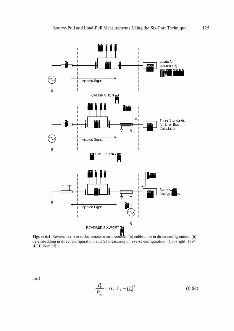
Source-Pull and Load-Pull Measurements Using the Six-Port Technique 125
Figure 6.4 Reverse six-port reflectometer measurements: (a) calibration in direct configuration; (b) de-embedding in direct configuration; and (c) measuring in reverse configuration. (Copyright 1994
IEEE from [9].)
and
266 6L
ref
PQ
P= α Γ − (6.6c)

126 The Six-Port Technique with Microwave and Wireless Applications
where iα and iQ are complex constants. The reflection coefficient LΓ of the load
is determined by the intersection of three circles using the six- to four-port
reduction technique similar to technique explained in Chapter 4 as
4
22*
4 44 4 4 5 4
2 * *55 5 5 5 5 5 5
*26 6 6 6 6
6 66
ref
L
Lref
L
ref
P
P Q Q QP
Q Q QP
Q QQP
P
α α −α −α Γ = α + α −α −α Γ α −α −α Γ α
(6.7a)
244 4
12 *
4 4 4 5 42* * 5
5 5 5 5 5 5 5
*
6 6 6 6 6
266 6
ref
L
Lref
L
ref
PQ
PQ Q
PQ Q Q
PQ Q
PQ
P
−
− α
Γ α −α −α Γ = α −α −α − α Γ α −α −α − α
(6.7b)
Examining (6.7), we note that the product of rows two and three is equal to row
one. Hence, after some algebraic manipulation, we eliminate LΓ and obtain the
following relation:
2 2 2
2 2 2 2 25 6 54 4
2 2 26 5 64
4
( ) ( ) ( )
( ) ( )
( )
ref ref ref ref ref
ref ref ref ref
ref
P P PP Pp q A r B r p q A
P P P P P
P P PPq p r B p q r A B
P P P P
Pp p q r
P
+ + + − − +
− − + − − +
− − +
2 25 6( ) ( ) 0ref ref
P Pq q p r A r r p q B pqr
P P
− − + − − + =
(6.8)
where the real quantities p, q, r, A2,B2 are the calibration constants related to iα
and iQ and associated with the physical structure of the six-port junction [10].
These parameters are determined by the six-port to four-port reduction theory:
for each specified frequency, at least five measurements for different distributed
loads that lead to a set of five nonlinear equations are needed to solve this set of

Source-Pull and Load-Pull Measurements Using the Six-Port Technique 127
equations [10,11]. The explicit knowledge of the impedance values of these
distributed loads is not required in the calculation of p, q, r, A2, and B2. As
discussed earlier, in practice, 13 loads are employed to improve the accuracy of
the calibration over the entire Smith chart.
The elimination of 2
2b in (6.5) makes the quantities p, q, r, A2, and B2
completely independent of the choice of port 1 or port 2 for the test port of the six-
port junction. Hence, if the power reference and the remaining detection ports are
fixed, the calibration of the six-port, which aims at the determination of p, q, r, A2,
and B2, will normally give the same value of these parameters for a six-port used
in either direct or reverse configurations.
6.3.2 Error Box Calculation for Reverse Six-Port Measurements
Once the calibration constants are found, the six-port can measure an embedded
reflection coefficient 2 2( , , , , , )i refw g P P p q r A B= at an unknown reference plane
[10]. The error box calculation (or de-embedding procedure) determines the three
complex constants c, d, and e, which relate w to the reflection coefficient, Γ, at a
chosen reference plane by the following relation:
1
d ew
c
Γ +=
Γ + (6.9)
With three well-known standards and with their measured embedded reflection
coefficients wi given by the six-port, one can easily find c, d, and e by solving the
linear system given here:
1 1 1 1
2 2 2 2
3 3 3 3
std std
std std
std std
w c d e w
w c d e w
w c d e w
Γ − Γ − = −
Γ − Γ − = −
Γ − Γ − = −
(6.10)
Referring to Figure 6.4(c), for a reverse six-port, the microwave signal must be
injected from the output port (port 2) to the input port (port 1) and we must
present the three de-embedding standards at the left side of the reference plane,
which is physically impossible. To overcome this difficulty, a direct six-port error
box, as shown in Figure 6.4(b), with the three standards connected successively to
the measuring port at the right side of the reference plane is used. For the reverse
six-port error box calculation, the system (6.10) is replaced by the following:

128 The Six-Port Technique with Microwave and Wireless Applications
1 1
1 1
2 2
2 2
3 3
3 3
std std
std std
std std
c dw e w
c dw e w
c dw e w
′ ′′− − = −
Γ Γ
′ ′′− − = −
Γ Γ
′ ′′− − = −
Γ Γ
(6.11)
where the value stdiΓ of the three standards in (6.10) are replaced by 1/ std
iΓ in
(6.11). Note that using the value of stdiΓ is equivalent to presenting these
standards at the left side of the reference plane, which is valid when Γ is referred
to the same characteristic impedance (50 Ω).
In practice, it is usually convenient to use a short circuit, an open circuit, and a
matched load of 50 Ω (Γ = 0) as the three de-embedding standards. Unfortunately,
for a reverse six-port error box procedure, the matched load needs to be replaced
by another standard to avoid the l/ Γ singularity. To circumvent this difficulty, one
can determine the reverse six-port error box by first finding the coefficients c, d, and e of the conventional error box procedure and next deducing the coefficient c', d', and e' of the reverse six-port error box using the following relations:
1/ ; 1/ ; 1/c c d d e e′ ′ ′= = = (6.12)
These relations can be easily derived by comparing the two sets of linear
equations, (6.10) and (6.11). Measurement results obtained by a reverse six-port
calibrated and de-embedded according to the above procedures confirm the
validity of this technique [9]. The reverse six-port reflectometer is suitable for
performing source-pull measurements at the input of the DUT. The measurement
technique consists of a signal injected into the DUT via the directional coupler.
The reflected signal from the input port of the DUT allows the six-port to perform
measurements in the opposite direction. It should be mentioned that when the
DUT is well matched, the six-port reflectometer will not be powered and will not
operate. However, source-pull measurements are only useful when the DUT input
is mismatched.
6.3.3 Discussion
In light of (6.9) and (6.12), we can easily see that 1/′Γ = Γ where ′Γ and Γ are,
respectively, the reflection coefficients measured by a six-port in reverse and in
direct configurations. It may seem that this relation can be equally obtained by just

Source-Pull and Load-Pull Measurements Using the Six-Port Technique 129
taking /b aΓ = and /a b′Γ = (where a and b are, respectively, the incident and
the reflected wave), but this is not true. For example, in the case of a direct six-
port measurement, .1/ measΓ does not lead to the impedance of the generator and
has no physical significance. In a direct six-port configuration, the DUT is
connected to port 2 of the six-port reflectometer that measures the ratio of 2 2/a b ,
the incoming and outgoing waves at the output of the junction (port 2, in Figure
6.10). This ratio 2 2/a b represents the reflection coefficient of the DUT, seen from
the left side of the reference plane. In a reverse six-port configuration, the
reference plane is always located at port 2 but the output port of the reflectometer
becomes port 1.
Thus, the reverse six-port junction measures the ratio of 1 1/a b rather than 2 2/a b .
The ratio 1 1/a b shifted to port 2 of the six-port junction by the de-embedding
procedure then represents the reflection coefficient of the test port of the six-port
reflectometer, seen from the load side of the reference plane. Therefore, the
inverse value 1 1/b a cannot yield the reflection coefficient of the device under test
connected to port 2. In summary, reverse six-port reflectometer measurements
require a conventional calibration procedure to characterize the six-port junction
and a special error box to fix the reference plane. This error box can be obtained
either by using the relations given by (6.12) or by inverting the actual reflection
coefficient Γ of the standards used to calculate the parameters c, d, and e of the
direct error box.
6.4 SOURCE-PULL CONFIGURATION USING SIX-PORT
The source-pull measurement is aimed at evaluating linear/nonlinear device
performance as a function of source impedance [1]. In source-pull measurement,
the input load varies as a load at the source side. The source-pull is measured
using six-port technique both in passive and active configurations.
6.4.1 Passive Source-Pull Configuration
The passive source-pull techniques are based on the use of a tuner. Figure 6.5
shows the setup for a passive source-pull: the input signal is injected into the
device under test (DUT) via a directional coupler, and the source impedance is set
with a stub tuner. The six-port in such an arrangement is operated in reverse
configuration and measures the source impedance seen at the reference plane.

130 The Six-Port Technique with Microwave and Wireless Applications
Figure 6.5 A passive source-pull measurement system.
6.4.2 Active Source-Pull Configuration
Figure 6.6 shows the setup for an active source-pull measurement. This setup uses
a variable attenuator and a variable phase shifter. The attenuator and phase shifter
values can be varied during the measurement.
Figure 6.6 An active source-pull measurement system.

Source-Pull and Load-Pull Measurements Using the Six-Port Technique 131
The six-port in this setup is used in reverse configuration allowing the
measurements of the source impedance seen at the reference plane. As may be
seen, the active source-pull configuration has more flexibility and accuracy in
comparison to the conventional passive source-pull technique.
6.5 LOAD-PULL CONFIGURATION USING SIX-PORT
The load-pull measurement evaluates linear/nonlinear device performance as a
function of load impedance. Both passive and active load-pull measurement
setups can be realized using the six-port technique.
6.5.1 Passive Load-Pull Configuration
The passive load-pull configuration, as shown in Figure 6.7, comprises two six-
port junctions, SP1 and SP2 and two tuners, T1 and T2. This configuration allows
SP1DUT
Ref 4 5 6
1 2 SP2
4 5 6
21
Ref
OUTINΓin
a1
b1
T1 T2
b2
a2
Figure 6.7 Six-port based passive load-pull measurement configuration.
the evaluation of a large-signal input impedance ( )in fΓ of the TUT and the
power delivered to it ( )inP f by means of SP1 as shown in the Figure 6.7.
The source impedance seen by the DUT at its input can be changed by varying
the stub positions of T1 as follows:
( ) ( )1 1 1in f b a fΓ = = Γ (6.13)

132 The Six-Port Technique with Microwave and Wireless Applications
( )( ) ( ) ( )( )
( ) ( )
2
1 12 2
1 1 2
1
11
( )2 1
r in
in
in
k f P f fP f a b
c f f
− Γ= − =
+ Γ (6.14)
In opposition to ( )in fΓ , the source impedance ( )s fΓ cannot be determined
online using the conventional calibration and measurement approaches describing
the operation of the six-port reflectometer in direct or forward mode. As
presented in the previous chapters, a straightforward technique to solve such a
problem is to perform a precalibration of T1 using a network analyzer that gives
the impedance of the tuner’s port connected to the TUT DUT as a function of the
tuner’s stub positions. This technique requires a repeatable and high quality
computer driven tuner.
The reflection coefficient associated with load impedance and the power
absorbed by the load, are measured with SP2 operated in direct configuration (port
1 is connected to the DUT and port 2 to the load) and can be calculated as follows:
( ) ( ) ( )2 2L f a f b fΓ = (6.15)
( )( ) ( ) ( )
( ) ( )
2
2 2 2 2
2 2 2
2
(1 )1( )
2 1
r L
L
L
k f P f fP f b a
c f f
− Γ= − =
+ Γ
(6.16)
SP2 operated in forward configuration provides the value of Γ2; consequently, ΓL
can be easily obtained as follows:
2
2 1L
Γ +Γ =
Γ +
α βδ
(6.17)
where α, β, and δ are the complex coefficients modeling the two-port network
delimited by the reference planes where ГL and Г2 are defined and measured. α, β,
and δ parameters can be determined beforehand using the short open load de-
embedding technique. Section 6.6 provides the necessary equations to de-embed
both the reflection coefficient and the power flow measurements between different
reference planes and through different error networks.
The passive source-pull tuning configuration, as shown in Figure 6.5, and
explained in section 6.3.1, allows the measurements of the source impedance,
which has to be retuned for every load impedance to maximize the power
absorbed by the DUT. In case of a DUT that can be considered unilateral (s12~0),
the position of this input tuner can fixed once for a maximum power transfer at the
input of the transistor (Γs= Γin*).

Source-Pull and Load-Pull Measurements Using the Six-Port Technique 133
6.5.2 Active Branch Load-Pull Configuration
The active load-pull measurement system is basically a six-port network analyzer
that incorporates two six-port junctions including phase and amplitude signal
controllers inserted in one branch. The active load-pull configuration is shown in
Figure 6.8.
(a)
φ
VG VD
1 2
SP1 SP2
Six-PortTuner
Six-Port
Attenuator
Power Divider
Source
Linear
Amplifier
Attenuator
Phase Shifter
IsolatorIsolator
(b)
Figure 6.8 Six-port based active load-pull measurement : (a) configuration and (b) measurement systems.
The two six-port junctions are calibrated independently for impedance and power
flow measurements in a reflection mode operation. The active load-presented to
the TUT, ( )LZ f , can be varied by changing the phase and the amplitude of the

134 The Six-Port Technique with Microwave and Wireless Applications
injected signal ( )2a f at the output of the TUT. The active load-pull measurement
system is presented in Figure 6.8.
The complex value of ( )LZ f can be deduced from the measured reflection
coefficient, ( )2fΓ , obtained by the second six-port reflectometer SP2 as follows:
( ) ( )( )0
1
1
LL
L
fZ f Z
f
+ Γ=
− Γ (6.18)
( )( )2
1L f
fΓ =
Γ
(6.19)
The absorbed power by the active (electronic) load presented to the DUT can be
calculated using the following expression:
( ) ( ) ( )
2
2 2LP f P f f= Γ
(6.20)
6.5.3 Active Loop Load-Pull Configuration
An alternative technique to realize active load-pull measurement is the active loop
method. The active loop architecture is shown in Figure 6.9; a directional coupler
placed at the output of the DUT (the loop coupler) takes part of the signal and
sends it to a variable attenuator, a phase shifter, a tunable filter, and an amplifier.
The loop also uses a circulator upstream from the amplifier. Then, the signal is re-
injected back in to the DUT output. In this configuration, the reflection coefficient
provided to the DUT does not change with the output power if the loop amplifier
is in the linear region and has a constant gain [2].
Figure 6.9 Six-port active loop load-pull measurement system.

Source-Pull and Load-Pull Measurements Using the Six-Port Technique 135
6.6 SOURCE-PULL/LOAD-PULL CONFIGURATION USING SIX-PORT
The source-pull/load-pull technique is a characterization method of DUT based on
the output performance’s optimization by tuning output and input impedances
seen at DUT accesses. Similar to the load impedance, the impedance of the source
providing the input signal for the DUT also plays a role in its behavior. The source
impedance presented at the device input can influence output characteristics like
linearity or optimum load impedance.
A passive source-pull/load-pull configuration is shown in Figure 6.10. The input
and output tuners may be replaced with active source and active load
configurations. To implement a source-pull/load-pull measurement system, the
source switch position 1 is used. In this position, the switch connects the source
signal in the load-pull configuration. In such a configuration, one can measure
directly (Γin, Pin) and (ΓL, PL) using SP1 and SP2 operated both in the forward
configuration for a fixed position of the input tuner presenting Γs to the input of
the DUT. Knowing ΓL, one can easily obtain Γout using (6.17) along with the
SOLT de-embedding technique to determine the three error box parameters.
1
Lout
L
Γ +Γ =
Γ +
α βδ
(6.21)
where α, β, and δ are the complex coefficients modeling the two-port network
delimited by the reference planes where ГL and Гout are defined and measured.
The Γs presented to the device can be determined by operating the input six-port
SP1 in reverse configuration through the appropriate setting of the three switches
connected to the input tuner, the generator, and the input directional coupler in
position 0.
outΓinΓ
LΓsΓ
tΓ
Figure 6.10 A block diagram of source-pull/load-pull configuration.
Hence, the source impedance can be varied and adjusted for any position of the
load impedance. Accordingly, the source-pull/load-pull provides a solution for
simultaneous measurement of both the input reflection coefficient of the device

136 The Six-Port Technique with Microwave and Wireless Applications
under test (DUT) and the reflection coefficient of the synthesized source with
variable impedance [1,3].
6.7 A DE-EMBEDDING TECHNIQUE FOR ON-WAFER LOAD-PULL
MEASUREMENTS
An absolute de-embedding technique for simultaneous impedance and power
measurements suitable for on-wafer load-pull measurements of microwave
transistors is proposed [1,3-7]. This technique allows one to perform impedance
and power calibration of a network analyzer directly from the embedded reflection
coefficient measurements. This technique requires two sets of open-short-load
calibration standards, one coaxial and one noncoaxial such as coplanar (CPW). An
absolute power calibration performed at the coaxial reference planes using a
standard power meter is also required for accurate power flow measurement
purposes at the coplanar reference planes of the microwave probes needed for on-
wafer measurements.
6.7.1 Calibration and Measurement Techniques
A general formulation of the problem is illustrated in Figure 6.11, where ( )A,B
are two error box networks delimited by the network analyzer reference planes
and the coaxial reference planes; ( )′ ′A , B are two error box networks delimited
by the coaxial reference planes and the coplanar reference planes at the tips of the
microwave probes. Let [ ] [ ]( )A , B and [ ] [ ]( )′ ′A , B designate the transmission
matrices of these two pairs of error box networks.
The reflection coefficients at both coaxial and coplanar reference planes are
related, respectively, to the reflection coefficients at the network analyzer
reference planes and the coaxial reference planes (see Figure 6.11) as follows:
Figure 6.11 On-wafer impedance and absolute power calibration procedure.
′Γ A
′P A
′PB
′Γ B
′ ′ΓB
ΓA
PA ′ ′ Γ A
ΓB
PB
DUT
A′′′′ A B′′′′ B
Tip probe planes
plan NA plane NA plane Coaxial plane Coaxial plane PSA
PSA

Source-Pull and Load-Pull Measurements Using the Six-Port Technique 137
1 2
3 1
AA
A
α Γ + α′Γ =
α Γ +
(6.22a)
1 2
3 1
AA
A
′ ′ ′α Γ + α′′Γ =
′ ′α Γ +
(6.22b)
1 2
3 1
BB
B
β Γ + β′Γ =
β Γ +
(6.22c)
1 2
3 1
BB
B
′ ′ ′β Γ + β′′Γ =
′ ′β Γ + (6.22d)
where iα , i′α , iβ , and i
′β are the error box parameters, which can be calculated
using four OSL calibrations, two at the coaxial reference planes and two at the
coplanar reference planes.
The two power flows at the coaxial reference planes can be calculated as follows
[6]:
2
31
A SAA
A
k PP
′′ =
′ ′+ α Γ (6.23a)
2
31
B SBB
B
k PP
′′ =
′ ′+ β Γ (6.23b)
where SAP and SBP are two power readings sampled by two directional couplers
as shown in Figure 6.1. These directional couplers can be placed within the
network analyzer or can be inserted between the coaxial reference planes and the
coplanar reference planes and Ak ′ , Bk ′ are power calibration factors which can be
calculated by connecting an absolute power meter successively at both coaxial
reference planes as follows:
( )
2
3
2
1
1
APM APMA
SAPM APM
Pk
P
′ ′+ α Γ′ =
′− Γ (6.24a)
( )
2
2
1
1
BPM BPMB
SBPM BPM
Pk
P
′ ′+ β Γ′ =
′− Γ (6.24b)
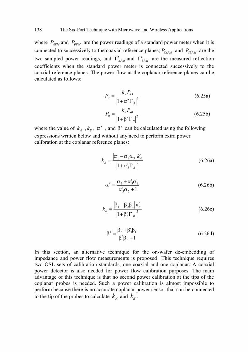
138 The Six-Port Technique with Microwave and Wireless Applications
where APMP and BPMP are the power readings of a standard power meter when it is
connected to successively to the coaxial reference planes; SAPMP and SBPMP are the
two sampled power readings, and APM′Γ and BPM
′Γ are the measured reflection
coefficients when the standard power meter is connected successively to the
coaxial reference planes. The power flow at the coplanar reference planes can be
calculated as follows:
21
A SAA
A
k PP =
′′+ α Γ
(6.25a)
21
B SBB
B
k PP =
′′+ β Γ (6.25b)
where the value of Ak , Bk , ′′α , and ′′β can be calculated using the following
expressions written below and without any need to perform extra power
calibration at the coplanar reference planes:
1 2 3
2
31
AA
A
kk
′α − α α=
′+ α Γ (6.26a)
3 3 1
3 2 1
′α + α α′′α =
′α α + (6.26b)
1 2 3
2
31
BB
B
kk
′β − β β=
′+ β Γ (6.26c)
3 3 1
3 2 1
′β + β β′′β =
′β β + (6.26d)
In this section, an alternative technique for the on-wafer de-embedding of
impedance and power flow measurements is proposed This technique requires
two OSL sets of calibration standards, one coaxial and one coplanar. A coaxial
power detector is also needed for power flow calibration purposes. The main
advantage of this technique is that no second power calibration at the tips of the
coplanar probes is needed. Such a power calibration is almost impossible to
perform because there is no accurate coplanar power sensor that can be connected
to the tip of the probes to calculate kA and kB .

Source-Pull and Load-Pull Measurements Using the Six-Port Technique 139
6.8 APPLICATIONS OF SOURCE-PULL MEASUREMENTS
In the conventional application of a six-port to characterize a DUT, the microwave
signal generator is connected to the input port, the DUT is connected to the output
port, and the four remaining measuring ports are used for power detection
purposes. This configuration allows the six-port to measure the power absorbed by
the device under test and of the generator has no effect on the measurement of the
six-port; therefore, it is impossible to get information about the effect of the
source impedance on the performance of the DUT.
In certain situations, such as in the characterization of mixers, oscillators, or
noise measurements, it is more desirable to vary the generator impedance and
measure its reflection coefficient than to measure the reflection coefficient of the
DUT. Such source-pull characterization is not possible, either by using an
automatic vector network analyzer or by using the conventional six-port
configuration. In this section, an approach for source-pull measurements of active
two-port devices using a six-port reflectometer in reverse configuration is
presented. The microwave source, the DUT, and the measuring reference plane
are all placed at the output of the six-port junction. A tuner is connected at the
input of the six-port junction. In this arrangement, the six-port can drive
simultaneously the input of the DUT and perform source-pull measurements.
6.8.1 Low Noise Amplifier Characterization
An important part of low noise amplifier design is the measurement of the
transistor’s noise figure and the determination of noise parameters. Figure 6.12
shows a setup for noise characterization using the reverse six-port source-pull
measurement technique. The six-port junction is calibrated at all test frequencies
and measures the source impedance seen by the DUT. Obviously, the microwave
generator must be turned off when the noise source is on for noise measurement
and vice versa. The stability of the DUT is also important during this
characterization. The noise figure can be determined using the noise source and a
noise meter and a standard measurement procedure.
The noise figure is obtained as [14]
10log DUT in addedDUT
DUT in
G N NNF
G N
+= (6.27)
where Nadded is the difference between measured output noise level and the noise
level at the input of the device, GDUT is the gain of the DUT, and Nin is the
available noise power at input of the DUT.

140 The Six-Port Technique with Microwave and Wireless Applications
Figure 6.12 Using a reverse six-port reflectometer for noise characterization. (Copyright 1995 IEEE
from [14].)
The advantage of the six-port source-pull based noise measurement is that the
six-port in reverse configuration gives the source impedance for any tuner position
without any need to premeasure and calibrate the tuner in advance using the
network analyzer. In addition in this setup tuner repeatability is not an issue at all.
6.8.2 Mixer Characterization
Mixers employ mostly the nonlinearity of the active device to generate
intermodulation products. Thus, their behavior depends strongly on the load and
the LO and RF source impedance terminations. Computer-aided design
approaches using harmonic balance methods allow the optimization of the input
and output matching impedances, but the accuracy of the analysis relies on the
device modeling.
In practice, it is possible to optimize, at the same time, the input and the output
impedances by using a reverse six-port reflectometer to perform source-pull
Source-Pull and Load-Pull Measurements Using the Six-Port Technique 141
Figure 6.13 Experimental setup for the source-pull characterization of MESFET gate mixer. (© 1994
from IEEE [9].)
measurements at the input and a direct six-port reflectometer to obtain load-pull
measurements [15] at the output of the DUT.
The mixer performance can be optimized by increasing its conversion gain, by
improving return losses at its ports or even its linearity. The advantage of the six-
port source-pull based mixer characterization is that the six-port in the reverse
configuration gives the source impedance for any tuner position without the need
to premeasure and calibrate the tuner in advance of using the network analyzer.
In addition, in this set-up tuner repeatability is not important. The experimental
source-pull/load-pull characterization of a GaAs MESFET as a mixer is shown in
Figure 6.13. This technique can be used to find the optimal input RF and LO load
impedances of a MESFET gate mixer. The measurement results of the
characterization of the mixer are presented in [9].
6.8.3 Power Amplifier Characterization
Figure 6.14 shows a common setup for power amplifier characterization. The use
of reverse six-port reflectometers allows for the measurement of the source and
load impedances presented to the transistor by input and output tuning.

142 The Six-Port Technique with Microwave and Wireless Applications
outΓ
inΓ
LΓ
sΓ
tΓ
Figure 6.14 Two reverse six-port reflectometers for power amplifier characterization.
The PA designer can verify the transistor sensitivity in power gain versus
termination impedances and can easily optimize the output power, the amplifier
gain, the power-added efficiency, or the intercept point of the transistor [16]. The
power relations are obtained as follows:
( ) ( )22
2 (1 )out LP f b f= − Γ
(6.28a)
( ) ( )22
1(1 )in inP f a f= − Γ
(6.28b)
out
in
PPower gain
P− =
(6.28c)
out in
dc
P PPAE
P
−=
(6.28d)
where it is assumed that the dissipated dc power is known to calculate the power-
added efficiency (PAE).
6.9 SOURCE-PULL/LOAD-PULL OSCILLATOR MEASUREMENTS
The characterization of active microwave devices is generally done by the
measurement of S parameters using automatic network analyzers (ANA). The test
port impedance of the ANA seen by the active device under test is the normal line
characteristic impedance of the measurement system (50Ω). It must be noted that
Source-Pull and Load-Pull Measurements Using the Six-Port Technique 143
such a test port impedance cannot normally be varied during measurements. This
constraint is not convenient when measuring active devices with a negative
resistance (e.g., diode, transistors, and so forth), because oscillations might occur
during characterization whenever the negative resistance of the device exceeds
50Ω. In this section a six-port reflectometer with variable test port impedance is
considered. The six-port junction was specially designed to allow the variation of
the test port impedance over almost the entire Smith chart. Such a reflectometer is
found suitable for a large signal active microwave device characterization such as
microwave source-pull/load-pull oscillator measurements [17].
6.9.1 Six-Port Reflectometer with Variable Test Port Impedance
By using the transparent six-port assumption, from (6.4) it can be seen that to
obtain a variation of the test port impedance, it is sufficient to vary the internal
impedance of the generator [17]. The variation of the test port impedance can be
performed by the use of a three-stub tuner inserted between the signal generator
and the input port of the six-port junction, as shown in Figure 6.2.
The generator and the three-stub tuner can be considered equivalent to a
generator with variable test port impedance. Based on the above consideration and
by using an appropriate calibration method, nonsensitive to the source power level
variation and to the internal source impedance [11], the calibration parameters of
the six-port reflectometer obtained for given tuner stub positions are valid for any
position of the stubs.
6.9.2 Oscillator Measurements
Source-pull/load-pull oscillator measurements monitor both the oscillator power
and the frequency as a function of the load impedance seen by the oscillator under
test. The impedance seen by the oscillator can be changed and, at the same time,
known over the quasi-entire Smith chart, by simultaneously changing and
measuring the test port impedance of the six-port junction.
Figure 6.15 shows a block diagram of an experimental setup for source-
pull/load-pull oscillator characterization using the reflectometer with variable test
port impedance. The reflection coefficient associated with the load impedance ZL
seen by the oscillator is directly deduced from the measured reflection coefficient
mΓ as follows:
1
1
mL o
m
Z ZΓ +
=Γ −
(6.29)

144 The Six-Port Technique with Microwave and Wireless Applications
Figure 6.15 A block diagram of the experimental setup for source-pull/load-pull oscillator
measurements. (© 1992 IEEE from [17].)
where oZ is the characteristic impedance of the measurement system (50Ω). The
available power Pa from the oscillator can be calculated using the six-port
calibration parameters and the power calibration parameter as follows [18]:
( )( ) ( ) ( )
( ) ( )
2
3
2
1
m
a
m
k f P f fP f
c f f
Γ=
+ Γ (6.30)
where ( )c f is the de-embedding calibration parameter obtained by the six-port
error box calibration at the oscillator frequency f, ( )k f is a scalar parameter
obtained by the power calibration at the oscillator frequency f, ( )3P f is the
power reading at port 3 of the six-port junction at the oscillator frequency f, and
( )m fΓ is the reflection coefficient measured by the six-port reflectometer at the
oscillator frequency f. The impedance seen by the oscillator can be simultaneously varied and measured
over the quasi-entire Smith chart by changing the tuner stub positions and
measuring the test port impedances of the six-port junction. The available power
from the oscillator under test Pa is easily obtained at any tuner stub position and at
any operating oscillator frequency using (6.29) and (6.30).
The oscillator frequency is measured by using a directional coupler and a
frequency counter as shown in Figure 6.15. The six-port reflectometer is
calibrated at discrete frequency points centered on the nominal oscillator
frequency. The measurement results of the characterization of an oscillator are
presented in [17].

Source-Pull and Load-Pull Measurements Using the Six-Port Technique 145
6.10 AM-AM/AM-PM DISTORTION MEASUREMENTS OF
MICROWAVE TRANSISTORS USING ACTIVE LOAD-PULL
Low phase distortion MESFET power amplifiers and limiters are key components
in systems where the information is related to the phase of the microwave signal.
For an accurate and quick design of linear solid state power amplifiers (SSPAs)
and power limiters in hybrid microwave integrated circuits (HMIC) and
monolithic microwave integrated circuits (MMIC) technologies, transistor
characterization in terms of phase distortion measurements is highly
recommended. The AM/PM distortion behavior can be described by the relative
phase shift versus input power, ( )inPφ and the AM/PM conversion coefficient k is
in degrees per dB. Various methods for measuring the AM-PM conversion
coefficients at intermediate frequencies have been published [19,20].
However, for microwave/millimeter wave amplifiers, it is less complex and
tedious to obtain the characteristic ( )inPφ , by single-carrier power sweep
measurements [21]. Then, if needed, k can be found by derivation of φ with
respect to ( / )in inP d dPφ . Actually, the measured ( )inPφ curve as a phase transfer
function is more general to characterize the AM-PM distortion performance of
microwave transistors and power amplifiers. In addition, the ( )inPφ
characterization is especially useful for microwave limiters, where the variation
range of the phase shift over a given power range beyond saturation is the main
concern [22].
This section presents an approach to simultaneously investigate the AM/PM
characteristics along with the AM-AM characteristics as the functions of the
power level and the load impedance over the Smith chart using the six-port. For a
designed performance in terms of output power, efficiency, and AM-PM
distortion, this comprehensive characterization can provide data for improving the
design of limiting amplifier or SSPAs driven by time-variable envelop signals.
The proposed approach is based on the principles of a dual six-port network
analyzer [21] and the active loading technique [23]. In comparison with the setups
employing heterodyne network analyzers, the advantages of this measurement
setup are: (1) the impedance and power measurements are performed at the actual
power level of the device, and no extra attenuators are needed for power device
characterization; (2) the AM-PM characterizations are carried out at the input and
output reference planes of the device under test, loaded by arbitrary impedances;
and (3) the cost of this system is much lower than the cost of the setups using two
automatic network analyzers for AM-PM distortion load-pull measurements.
6.10.1 Principle of Operation
The measurement system is shown in Figure 6.16. As shown, two six-port
junctions, associated with the amplitude and phase controllers, can be utilized for

146 The Six-Port Technique with Microwave and Wireless Applications
Figure 6.16 Block diagram of load-pull phase of distortion measurement system. (© 1995 IEEE from
[21].)
active load-pull techniques. Meanwhile, the measurement system can be viewed
as a three-port network with reference planes 1, 2, and 3. In order to measure the
input-output phase shift of the transistor under test (TUT), three two-port passive
standards, Z1, Z2, and Z3, are introduced to obtain a calibration coefficient. Due
to the fact that the three-port network has fixed network scattering parameters
during the four measurements of the TUT, Z1, Z2, and Z3 for a fixed setting of
the amplitude and phase controllers, we can obtain the following equations
expressed in matrix format [10].
12 1 22 12 1 1 1 11
12 1 22 12 1 2 1 11
12 1 22 12 1 3 1 11
(1) (1) (1) (1) (1) (1) (1) (1)
(2) (2) (2) (2) (2) (2) (2) (2)
(3) (3) (3) (3) (3) (3) (3) (3)
S S S x S
S S S x S
S S S x S
∆ − Γ Γ Γ − ∆ − Γ Γ = Γ − ∆ − Γ Γ Γ −
(6.31)
where xi is related to scattering parameters of the three-port network for a given
amplitude and phase setting; 11 22 12 21
( ) ( ) ( ) ( ) ( )k S k S k S k S k∆ = − and ( )ijS k k, = 1,
2, and 3 are the known S parameters of three standards Z1, Z2, and Z3. Γ1(k), k = 1,
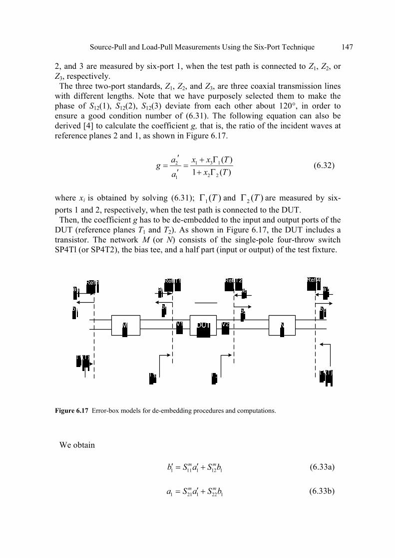
Source-Pull and Load-Pull Measurements Using the Six-Port Technique 147
2, and 3 are measured by six-port 1, when the test path is connected to Z1, Z2, or
Z3, respectively.
The three two-port standards, Z1, Z2, and Z3, are three coaxial transmission lines
with different lengths. Note that we have purposely selected them to make the
phase of S12(1), S12(2), S12(3) deviate from each other about 120°, in order to
ensure a good condition number of (6.31). The following equation can also be
derived [4] to calculate the coefficient g, that is, the ratio of the incident waves at
reference planes 2 and 1, as shown in Figure 6.17.
1 3 12
2 21
( )
1 ( )
x x Tag
x Ta
′ + Γ= =
+ Γ′ (6.32)
where xi is obtained by solving (6.31); 1( )TΓ and
2 ( )TΓ are measured by six-
ports 1 and 2, respectively, when the test path is connected to the DUT.
Then, the coefficient g has to be de-embedded to the input and output ports of the
DUT (reference planes T1 and T2). As shown in Figure 6.17, the DUT includes a
transistor. The network M (or N) consists of the single-pole four-throw switch
SP4Tl (or SP4T2), the bias tee, and a half part (input or output) of the test fixture.
Figure 6.17 Error-box models for de-embedding procedures and computations.
We obtain
1 11 1 12 1
m mb S a S b′ ′= + (6.33a)
1 21 1 22 1
m ma S a S b′= + (6.33b)

148 The Six-Port Technique with Microwave and Wireless Applications
and
2 11 2 12 2
n na S b S a′= +
(6.34a)
2 21 2 22 2
n nb S b S a′ ′= +
(6.34b)
where mijS and n
ijS are the S parameters of the networks M and N. Also, we have
1 1 1( ) /T b a′ ′Γ = and2 2 2( ) /T b a′ ′Γ = . From the above equations, a2/a1 can be
developed and related to coefficient g as follows:
2 12 2 11
1 21 1 22
( ). .
( )
m n n
n m m
a S T Sg
a S T S
Γ − ∆=
Γ − ∆
(6.35)
where 11 22 12 21
m m m m mS S S S∆ = − and 11 22 12 21
n n n n nS S S S∆ = − . Since the switches SP4T1
and SP4T2 are operated under linear conditions, the S parameters of networks M and N are constants when Pin, sweeps, and they can be obtained using de-
embedding method such as TRL [24].
According to the definition of the normalized waves a and b, the ratio of the
voltages at the output and input ports of the DUT for any arbitrary load at a given
Pin is determined as follows:
2 2 2 2
1 1 1 1
1 1/.
1
L
in
V a b a
V a b a
+ + Γ= =
+ + Γ
(6.36)
where2 1/a a is obtained by (6.35), inΓ is the input reflection coefficient of the
DUT, and LΓ is the load reflection coefficient presented to the TUT.
In brief, by means of the switches, 1(1)Γ ,
1(2)Γ , 1(3)Γ ,
2 (1)Γ , 2 (2)Γ ,
2 (3)Γ , 1( )TΓ , and
2 ( )TΓ can be measured when the Z1, Z2, Z3 and DUT are
inserted in turn for a fixed setting of the amplitude and phase controllers.
Meanwhile, it’s easy to obtain inΓ , Pin and LΓ , PL with the de-embedding
techniques when 1( )TΓ and
2 ( )TΓ are measured by six-port 1 and six-port 2
[13]. Therefore, the phase shift of the DUT can be determined by (6.31 through
6.36). The harmonics are filtered, as shown in Figure 6.14, to ensure that the
signals detected by the power-meter are the fundamental components only.
The phase distortion, φ , is defined as an input-output phase shift, relative to the
reference phase shift value at a given lower input power ref
inP (small-signal
operation mode) for a given load impedance. Thus, the pertinent relative phase
shift corresponds to the change of the angle of V2/V1 when Pin increases. The

Source-Pull and Load-Pull Measurements Using the Six-Port Technique 149
measurement ( ( )inf Pφ = ) of the AM-PM distortion behavior, followed by the
calculation of the derivative ( / )ind dPφ , provides the AM-PM conversion
coefficient. Similarly, the AM-AM distortion is described by the deviation of the
gain from its value at a small-signal input power level. Due to the fact that PL and
Pin are already measured, the operating power gain ( ( )p inG g P= ) can be deduced
and the AM-AM conversion coefficient can be determined by the derivative
( / )p indG dP [19, 21].
6.10.2 Measurement Procedure
Traditionally, the load-pull has to be carried out for each given Pin with
variable LΓ . This results in a large number of measurements and adjustments. The
present experimental procedure performs the active load-pull measurements by
fixing the positions of the amplitude and phase controllers and sweeping the input
power. In such conditions LΓ changes, as Pin is swept. Then, the amplitude and
phase controllers are adjusted at new positions and the measurements are
performed with another sweep of Pin. Finally, the load-pull contours for a given
Pin can be extracted from the recorded measurement database.
In addition, the characteristics ( L inP P∼ ) and ( inPφ ∼ ) for a given LΓ can be
obtained as a postmeasurement calculation result. The power-added efficiency
PAE and GP can also be deduced. It is known that in an active load-pull system,
when Pin changes it is difficult to maintain the required LΓ value by adjusting the
amplitude and phase controllers. This problem can be circumvented by means of
the above alternative procedure. The error sources in the proposed approach are
mainly due to the following four aspects. First, the measurements are made by
increasing the input power and not by amplitude modulation as in the actual
operation mode. Therefore, the dynamic effect of the AM modulation, which
becomes more significant by increasing the modulation bandwidth, is ignored.
Second, the self-heating effect can introduce a drift in the electrical operational
conditions. To minimize this effect, the temperature of the fixture of the transistor
investigated has to be maintained almost constantly by circulating a flux of air
during characterization. Third, the measurement accuracy can also be diminished
if the power level exceeds the operational range where the switches are linear. It is
preferable to use mechanical switches instead of solid-state switches when
characterizing high-power devices. Fourth, the extraction of the pertinent data
from the raw database and the postmeasurement calculations using interpolation
routines might introduce error. This effect can be reduced by increasing the
amount of experimental data.

150 The Six-Port Technique with Microwave and Wireless Applications
6.11 TIME-DOMAIN WAVE-CORRELATOR FOR POWER AMPLIFIER
CHARACTERIZATION AND OPTIMIZATION
Time-domain waveform measurement techniques are considered one of the most
useful methods for characterizing nonlinear microwave devices and amplifiers.
This is especially important for switching-mode and harmonic-controlled circuits.
The principle of highly efficient operation is to allow for a specific amount of
higher harmonic content in the current and voltage waveforms at the transistor
output terminals. In this way, power dissipation in the device is minimized by
avoiding the simultaneous presence of high currents and voltages in the device.
In order to verify proper operating conditions or to tune a circuit, it is essential to
measure and analyze the waveforms. Moreover, information about the amount of
magnitude and phase of spectral components in the output waveforms of a
nonlinear device under a large-signal stimulus is important for a better
understanding of the electrical behavior and for accurate large signal modeling of
the device under test (DUT). At microwave and millimeter frequencies, high-
speed sampling oscilloscopes [25], special vector network analyzer (VNA) setups,
optical sampling systems [26], and microwave transition analyzer (MTA)
techniques [27, 28] have been used.
In this section, an approach for high-frequency time-domain voltage and current
waveform measurements using six-port junction is described [29]. The advantage
of this waveform measurement setup is its relatively low implementation cost
compared to all the above-mentioned measurement techniques, especially at
millimeter-wave frequencies.
6.11.1 Time-Domain Waveform Measurement
One method of determining time-domain voltage and current waveforms consists
of measuring the complex Fourier coefficients of the waves in the frequency
domain. By accurately determining the magnitude of the dc component (Vo , Io), as
well as the magnitude and phase of the fundamental (V1, I1) and harmonic
frequency components (Vn, In), the time-domain waveforms can be calculated
from the measured coefficients by using the well-known inverse Fourier
transformation
02
0
( ) Re m
j nf tn
n
v t V e π
=
= ∑ (6.37)
and
02
0
( ) Re m
j nf tn
n
i t I e π
=
= ∑ (6.38)
where n denotes the harmonic order, f0 is the fundamental frequency, and m is the
total number of included harmonics. The dc components, Vo, Io, are routinely

Source-Pull and Load-Pull Measurements Using the Six-Port Technique 151
measured directly with a biasing instrument; however, the measurement of the
complex Fourier coefficients Vn, In for 1n ≥ is more difficult. Here, these
measurements with a deliberately modified six-port reflectometer have been
performed. To be able to determine the waveforms at the DUT output plane, the
measurement of the complex voltage traveling waves, also called pseudo-waves
[30], is performed at the fundamental (f0 ) , second (2f0 ), and third (3f0 ) harmonic
frequencies.
At a given reference plane, Vn and In in (6.33) and (6.34) are related to the
incident and reflected voltage traveling waves by [30,31]
n n nV a b= + (6.39)
and
n nn
c
a bI
Z
−= (6.40)
where Zc is the characteristic impedance of the system, typically 50Ω. By
measuring the pseudo-reflection coefficient n n na bΓ = , the magnitude and phase
of the voltage traveling wave an can easily be determined if the voltage traveling
wave bn is delivered by a reference generator, that is, its magnitude and phase of
its harmonic contents are well known. By measuring the pseudoreflection
coefficient nΓ at a given reference plane by means of a six-port reflectometer, the
voltage and the current frequency components can be deduced according to (6.39)
and (6.40). A multiharmonic generator is used to generate the harmonic-rich voltage wave
with well-known magnitude and phase components, as a reference signal
generator for the time-domain waveform calibration [29]. It is preferable that the
reference generator consists of a step recovery diode (SRD) excited by a
continuous wave (CW) RF signal at the fundamental frequency GHz. In most
cases, to reach an adequate input drive level for the SRD, a high-gain amplifier is
required.
6.11.2 Multiharmonic Six-Port Reflectometer
As discussed in Chapter 3, six-port junctions are in most cases designed using
directional couplers and power dividers that can cover several octaves of
bandwidth. However, the detection block of a conventional six-port reflectometer
is not able to discriminate the different spectral components because it only
detects the total power at the detection ports. Time-domain waveform
measurements, however, require the measurement of a few complex Fourier

152 The Six-Port Technique with Microwave and Wireless Applications
coefficients of the signal. In order to perform this measurement, the power
detection block of the six-port reflectometer is modified, as shown in Figure 6.18,
to become frequency selective and, hence, allow for multiharmonic
measurements.
The power detection block consists of a single-pole-four-through (SP4T) switch,
a tunable yttrium–iron–garnet (YIG) filter, and a power meter. For harmonic
measurements, the YIG filter is adjusted to pass only one harmonic frequency
component at a time from the output of the SP4T switch to the power meter.
Using the SP4T switch to successively switch from Ports 3 to 6 and detect the
powers, the reflection coefficient Γ = b/a can be measured in magnitude and phase
according to (6.37). The measurement procedure is detailed next. The YIG filter is
centered at f0. Port 3 is selected by means of the switch SP4T and the power is
measured. Before tuning the YIG filter to 2f0 , the powers at Port, 4, 5, and 6 are
measured. In the following measurement cycle, the filter is adjusted to 2f0 and the
powers at Ports 3, 4, 5, and 6 are determined. Finally, the filter is set to 3f0 and the
power detection steps are repeated.
Before every measurement, the repeatability of the YIG filter adjustment and the
switch contact quality has to be checked. The multiharmonic six-port
reflectometer is calibrated at f0, 2f0, and 3f0. The relationship between the
measured powers at Ports 3, 4, 5, and 6 (P3n, P4n, P5n, and P6n ) and the output
power, POUT n and the reflection coefficient, ΓLn , are given by [29]:
2
3 3
1
1
in in snin
n n sn
P Ak
P A
+ Γ=
+ Γ
(6.41)
where 1
sn
Ln
Γ =Γ
and
23
3
(1 )1
nOUTn Pn Sn
n sn
PP k
A= − Γ
+ Γ (6.42)
ink and inA (for i = 4, 5, 6) are determined by the six-port calibration procedure.
The constants Pnk are determined by an absolute power calibration method using a
reference power meter; n represents the harmonic order.
The six-port reflectometer calibration principles for time-domain voltage and
current waveform measurements are shown in Figure 6.19. The Fourier
coefficients of the harmonic-rich reference voltage wave An generated by Gref
have to be well known in both magnitude and phase. Unlike An, the spectral

Source-Pull and Load-Pull Measurements Using the Six-Port Technique 153
content of Bn, generated by Gunk, does not have to be known. Therefore, it can be
any arbitrary multiharmonic generator [29].
Figure 6.18 Multiharmonic SP reflectometer topology. (© 2008 IEEE [29].)
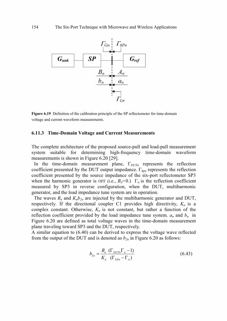
154 The Six-Port Technique with Microwave and Wireless Applications
Figure 6.19 Definition of the calibration principle of the SP reflectometer for time-domain
voltage and current waveform measurements.
6.11.3 Time-Domain Voltage and Current Measurements
The complete architecture of the proposed source-pull and load-pull measurement
system suitable for determining high-frequency time-domain waveform
measurements is shown in Figure 6.20 [29].
In the time-domain measurement plane, ΓDUTn represents the reflection
coefficient presented by the DUT output impedance. Γ6pn represents the reflection
coefficient presented by the source impedance of the six-port reflectometer SP3
when the harmonic generator is OFF (i.e., Bn=0.) Γn is the reflection coefficient
measured by SP3 in reverse configuration, when the DUT, multiharmonic
generator, and the load impedance tune system are in operation.
The waves Bn and Knb2n are injected by the multiharmonic generator and DUT,
respectively. If the directional coupler C1 provides high directivity, Kn is a
complex constant. Otherwise, Kn is not constant, but rather a function of the
reflection coefficient provided by the load impedance tune system. an and bn in
Figure 6.20 are defined as total voltage waves in the time-domain measurement
plane traveling toward SP3 and the DUT, respectively.
A similar equation to (6.40) can be derived to express the voltage wave reflected
from the output of the DUT and is denoted as b2n in Figure 6.20 as follows:
2
6
( 1)
( )
n DUTn nn
n Pn n
Bb
K
Γ Γ −=
Γ − Γ (6.43)

Source-Pull and Load-Pull Measurements Using the Six-Port Technique 155
Figure 6.20 Complete architecture of the proposed source-pull and load-pull measurement system
suitable for determining high-frequency time-domain waveform measurements. (© 2008 IEEE [29]. )
Whereas Bn in (6.43) has been determined in the calibration procedure by
replacing the DUT with a reference generator, Kn, ΓDOUTn, and Γ6pn need to be
measured with either a six-port reflectometer or a VNA. b2n can now be
determined and can be calculated according to
2 2n n Lna b= Γ
(6.44)
where LnΓ is measured by the six-port reflectometer SP2 in Figure 6.20. A
drawback of measurement systems using SP reflectometers in a reverse
configuration is the drastic loss of measurement accuracy in a 50Ω environment.
This is not an issue, however, for source-pull and load-pull systems since the
impedance levels are typically different form the system reference impedance,
ensuring sufficient precision for the reflection coefficient measurement in the
proposed setup. Finally, voltage and current waveforms at the DUT output port
are obtained using (6.39) and (6.40) as follows:
2 2n n nV b a= + (6.45)
156 The Six-Port Technique with Microwave and Wireless Applications
2 2n nn
C
a bI
Z
−= (6.46)
Depending on the bandwidth of the six-port junction, the frequency selective
detection module, and the fundamental frequency, in most cases measurements of
V and I at three to five harmonics are sufficient to determine the shape of time-
domain voltage and current waveforms accurately for amplifier design
applications.
The instantaneous voltage VDUT and the current IDUT waveforms at the output
terminal of the DUT are given by
0
32
0
( ) Re j nf t
DUT nn
V t V e π
=
= ∑ (6.47)
and
0
32
0
( ) Re j nf t
DUT nn
I t I e π
=
= ∑
(6.48)
and Vn, In (n=1,2,3 ) are measured with SP2 and SP3, whereas V0, I0 are measured
with a bias instrument. This setup was implemented and used for a medium-power
device optimized for maximum efficiency to demonstrate the capability of the
measurement system.
Time-domain voltage and current waveform measurements were performed with
the setup and compared to those obtained with a microwave transition analyzer
(MTA) based system. The measured time-domain voltage and current waveforms
at the output terminal of the FET are presented in Figure 6.21. The maximum
relative error of the measured waveforms is approximately 4% [29].

Source-Pull and Load-Pull Measurements Using the Six-Port Technique 157
Figure 6.21 Comparison of voltage and current waveforms measured with the time-domain setup and
an MTA. (a) Voltage waveform. (b) Current waveform. (© 2008 IEEE [29].)
References
[1] Le, D., and F. M. Ghannouchi, “Multitone Characterization and Design of FET Resistive Mixers
Based on Combined Active Source Source–Pull Load–Pull Techniques,” IEEE Trans. Instrument Meas., Vol. 46, No. 9, pp. 1201–1208, September 1998.
[2] Teppati, V., A. Ferrero, and U. Pisani, “Recent Advances in Real-Time Load-Pull Systems,”
IEEE Trans. on Instrumentation and Measurement, Vol. 57, pp. 2640–2646, November 2008.
[3] Berghoff, G., E. Bergeault, B. Huyart, and L. Jallet, “Automated Characterization of HF Power
Transistors by Source–Pull and Multiharmonic Load–Pull Measurements Based on Six-Port

158 The Six-Port Technique with Microwave and Wireless Applications
Techniques,” IEEE Trans. on Microwave Theory and Techniques, Vol. 46, No. 12, pp. 2068–
2073, December 1998.
[4] Soares, R. A., P. Gouzien, P. Legaud, and G. Follot, “A Unified Mathematical Approach to
Two-Port Calibration Techniques and Some Applications,” IEEE Trans. Microwave Theory Tech., Vol. MTT-37, pp. 1660–1674, November 1989.
[5] Ghannouchi, F. M., F. Beauregard, R. Hajji, and A. Brodeur, “A De-Embedding Technique for
Reflection-Based S-Parameters Measurements of HMICs and MMICs,” Microwave & Optical Tech. Letters, Vol. 10, No. 4, pp. 218–222, November 1995.
[6] Ghannouchi, F. M., G. Zhao, and F. Beauregard, “Simultaneous Load-Pull of Intermodulation
and Output Power Under Two Tone Excitation for Accurate SSPA Design,” IEEE Trans. Micro. Theory & Tech, Vol. 42, No. 6, pp. 943–950, June 1994.
[7] Ferrero, A., and U. Pisani, “An Improved Calibration Technique for On-Wafer Large-Signal
Transistor Characterization,” IEEE Trans. Inst. & Meas., Vol. 42, No.2, pp. 360–364, April 1993.
[8] Somlo, P. I., and J. D. Hunter, “Microwave Impedance Measurement,” IEE Electrical Measurement Series 2, London: Peter Peregrinus, 1985.
[9] Luan, D., and F. M. Ghannouchi, “Source-Pull Measurements Using Reverse Six-Port
Reflectometers with Application to MESFET Mixer Design,” IEEE Trans. Microwave Theory Tech., Vol. 42, pp. 1589–1595, 1994.
[10] Hodgetts, T. E., and G. J. Griffin, “A Unified Treatment of the Six-Port Reflectometer
Calibration Using a Minimum of Standards,” Royal Signals and Radar Establishment Rep. No. B3003, 1983.
[11] Engen, G. F., “Calibrating the Six-port Reflectometer by Means of Sliding Terminations,” IEEE Microwave Theory Tech., Vol. 26, pp. 951–957, December 1978.
[12] Hunter, J. D., and P. I. Somlo, “Explicit Six-Port Calibration Method Using Five Standards,”
IEEE Microwave Theory Tech., Vol. MTT-33, pp. 69–72, January1985.
[13] Engen, G. F., “The Six-Port Reflectometer: An Alternative Network Analyzer,” IEEE Microwave Theory Tech., Vol. 25, pp. 1075–1080, December 1977.
[14] Le, D., and F. M. Ghannouchi, “Noise Measurements of Microwave Transistors Using an
Uncalibrated Mechanical Stub Tuner and a Built-In Reverse Six-Port Reflectometer,” IEEE Trans. Instrument Meas., Vol. 44. No. 4, pp. 847–852, August 1995.
[15] Ghannouchi, F. M., R. Larose, and R. G. Bosisio, “A New Multiharmonic Loading Method for
Large Signal Microwave Transistor Characterization,” IEEE Microwave Theory Tech., Vol. 39,
pp. 986–992, June 1991.
[16] Gonzalez, G., Microwave Transistor Amplifiers Analysis and Design, Second Ed., Englewood
Cliffs, NJ: Prentice-Hall, 1996.
[17] Ghannouchi, F. M., and R. G. Bosisio, “Source-Pull/Load-Pull Oscillator Measurements at
Microwave/MM Wave Frequencies,” IEEE Trans. Instrument Meas., Vol. 41, pp. 32–35,
February 1992.
[18] Yakabe, T., M. Kinoshita, and H. Yabe, “Complete Calibration of a Six-Port Reflectometer with
One Sliding Load and One Short,” IEEE Trans. Microwave Theory Tech., Vol. 42, pp. 2035–
2039, November 1994.
[19] Koyama, K., T. Kawasaki, and J. E. Hanely, “Measurement of AM-PM Conversion
Coefficients,” Telecommun., Vol. 12, No. 6, pp. 25–28, June 1978.

Source-Pull and Load-Pull Measurements Using the Six-Port Technique 159
[20] Moss, J. F., “AM-AM and AM-PM Measurements using the PM Null Technique,” IEEE Trans. Microwave Theory Tech ,Vol. MTT-35, No. 8, pp. 780–782, 1987.
[21] Ghannouchi, F. M., G. Zhao, and F. Beauregard, “Simultaneous AM-AM/AM-PM Distortion
Measurements of Microwave Transistors Using Active Load-Pull and Six-Port Techniques,”
IEEE Trans. Microwave Theory Tech. Vol. 43, No.1, pp.1584–1588, July 1995.
[22] Parra, T., et al., “X-Band Low Phase Distortion MMIC Power Limiter,” IEEE Trans. Microwave Theory Tech. Vol. 41, No. 5, pp. 876–879, 1993.
[23] Ghannouchi, F. M., and R. G. Bosisio, “An Automated Millimeter-Wave Active Load-Pull
Measurement System Based on Six-Port Techniques,” IEEE Trans. Instrum. Meas., Vol. 41, No.
6, pp. 957–962, 1992.
[24] Engen, G. F., and C. A. Hoer, “Thru-Reflect-Line: An Improved Technique for Calibrating the l
Dual Six-port Automatic Network Analyzer,” IEEE Trans. Microwave Theory Tech., Vol. MTT-
27, pp. 987–993, 1979.
[25] Sipila, M., K. Lehtinen, and V. Pora, “High Frequency Periodic Time-Domain Waveform
Measurement System,” IEEE Trans. Microw. Theory Tech., Vol. 36, No. 10, pp. 1397–1405,
October 1988.
[26] Weiss, M., and Z. Popovic, “Time-Domain Optical Sampling of Nonlinear Microwave Power
Amplifiers,” IEEE MTT-S Int. Microw. Symp. Dig., pp. 889–892, June 1999.
[27] Raay, F. V., and G. Kompa, “A New On-wafer Large-Signal Waveform Measurement System
with 40 GHz Harmonic Bandwidth,” IEEE MTT-S Int. Microw. Symp. Dig., pp. 1435–1438, June
1992.
[28] Verspecht, J., P. Debie, A. Barel, and L. Martens, “Accurate on Wafer Measurement of Phase
and Amplitude of the Spectral Components of Incident and Scattered Voltage Waves at the
Signal Ports of Nonlinear Microwave Device,” IEEE MTT-S Int. Microw. Symp. Dig., pp. 1029–
1032, May 1995.
[29] Bensmida, S., P. Poiré, R. Negra, F. M. Ghannouchi, and G. Brassard, “New Time-Domain
Voltage and Current Waveform Measurement Setup for Power Amplifier Characterization and
Optimization,” IEEE Trans. Microwave Theory Tech., Vol. 56, No. 1, pp. 224–231, January
2008.
[30] Marks, R. B., and D. F. Williams, “A General Waveguide Circuit Theory,” J. Res. Nat. Inst. Standards Technol., Vol. 97, No. 5, pp. 533–562, September 1992.
[31] Verspecht, J., “Large-Signal Network Analysis,” IEEE Microwave, vol. 6, no. 4, pp. 82–92,
December 2005.

161
Chapter 7
Six-Port Wireless Applications
There is increasing demand for reduced complexity and power consumption in the
design of wireless terminals. Furthermore, wideband, compact-sized, and low-cost
digital transceivers are required to expand mobile and wireless communications.
Use of a multiport homodyne technique is interesting in wireless communications
due to the utilization of power detectors instead of mixers. This technique
provides simpler circuits in comparison with its heterodyne counterpart. The
advantages of such an approach are manifold. First of all, the broadband
specifications can be easily achieved by passive elements. Moreover homodyne
technique ensures low power consumption. In addition, its hardware architecture
is proposed as a means to avoid more costly transceivers. The objective of this
chapter is to study the multiport transceivers and their wireless applications.
7.1 MULTIPORT TRANSCEIVER
In this section, the operation of multiport structures as modulators and
demodulators is discussed.
7.1.1 Multiport Modulator
In a multiport modulator, some versions of the LO signal under various
amplitudes/phase angles are discussed, where the amplitude and phase of the
collected signal are properly achieved. The multiport transmitter uses some
variable reflectors and one collector, instead of conventional mixers. Figure 7.1
shows the functional block diagram of a multiport modulator, which consists of
one input, one output, and N reflection ports. The input signal is the local
reference signal, ( )LOa t . The multiport structure produces N various versions of
the LO signal and combines them in the output ports.

162 The Six-Port Technique with Microwave and Wireless Applications
|S31|ej 311
3
2
aLO
aRF
11
N
12
1M
N1
N2
NM
|S23|ej
|SN1|ej N1
|S2N|ej 2N
Modulation
Control
Figure 7.1 Functional block diagram of an N-port modulator.
The multiport junction is assumed to be a linear network, so the output signal of
the multiport structure is as follows:
1
2
1 2
1
1 1
2 2
, 1, 2,...,
i
i
Nk
RF i i i LOi
ji i
ji i
a S S a k M
S S e
S S e
=
= Γ =
=
=
∑φ
φ
(7.1)
where ijS are the scattering parameters of the multiport structure, and kiΓ is the
kth value of the reflection coefficient at the ith port using K reflection states. The
input and output signals are shown as LOa and RFa , respectively. For a specific
multiport structure, where the scattering parameters are given, the distinct values
for kiΓ can be calculated for each desired modulation scheme.
Figure 7.2 is a diagram of the six-port direct QPSK modulator. It consists of a
six-port circuit, a switch matrix, and open and short terminations. The circuit
operates as follows: port 1 is fed with a carrier signal, which is routed to ports 3,
4, 5, and 6 through the different branches of the six-port circuit. Signals present at
ports 3 to 6 are routed to different terminations by the switch matrix, controlled by
baseband data.

Six-Port Wireless Applications 163
Six-Port
Switch Matrix
Termination
Modulated
Signal
3 4 5 6
21
Figure 7.2 Six-port direct modulator architecture.
Those reflected signals are then summed at port 2, which is the output for the
modulated signal. The output signal acquires different phases depending on the
terminations applied at ports 3–6 [1]. A six-port direct 16QAM modulator is also
recently introduced by the use of a similar concept [2].
7.1.2 Multiport Demodulator
In a multiport demodulator, the received RF signal is summed with a local
oscillator signal under various phase angles. The multiport receiver uses power
detectors instead of conventional mixers. Figure 7.3 shows the functional block
diagram of a multiport demodulator, which consists of two inputs and N outputs.
The input signal is the received RF signal, a
RF(t) , and the local reference signal is
a
LO(t) .
The multiport structure produces N various combinations of RF and LO signals
and directs them to N power detectors. Therefore, N scalar outputs can be
obtained. The multiport junction is assumed to be a linear network. The N signal
levels off the multiport structure outputs, detected using Schottky diode detectors,
and the expression of demodulation equations can be derived as:
1
N
i oii
I Pα=
=∑ (7.2a)
1
N
i oii
Q Pβ=
=∑ (7.2b)

164 The Six-Port Technique with Microwave and Wireless Applications
Figure 7.3 Functional block diagram of an N-port demodulator.
where I and Q are the in-phase and quadrature components of the modulated
signal, and α
i and
β
iare the demodulation coefficients.
7.2 SIX-PORT RECEIVER
A multiport receiver consists of two inputs and N outputs. In direct-conversion
receiver applications, the RF and LO signals are applied to two input ports as two
complex inputs shown in Figure 7.4. The multiport structure produces N various
combinations of RF and LO signals and injects them to N power detectors, so that
N outputs can be obtained [3, 4]. If the multiport junction is a linear network, N
outputs of the multiport structure will be as follows:
2
1 2 1,2,...,i i LO i RFP S a S a i N= + =
(7.3a)
1
1 1ij
i iS S e φ= (7.3b)

Six-Port Wireless Applications 165
Figure 7.4 Direct conversion receiver based on six-port.
2
2 2ij
i iS S e φ= (7.3c)
where Sij is the scattering parameter of the multiport structure. Assuming that the
RF signal with digital modulation has the same frequency as the LO signal, the RF
and LO signals can be represented by:
1
2
LOjLO LOa a e ϕ=
(7.4)
2 21
2
RFjRF RFa a I Q e ϕ= +
(7.5)
where I and Q are in-phase and quadrature-phase modulating signals. By
substituting (7.4) and (7.5) in (7.3) and by use of the relations:
( )2 2 cos RFI I Q= + ϕ (7.6a)
( )2 2 sin RFQ I Q= − + ϕ (7.6b)
the expressions of output powers can be derived as

166 The Six-Port Technique with Microwave and Wireless Applications
( )( ) ( )( )
2 2 2 2 2 21 2
1 2
1 1
2 2
cos sin
i i LO i RF
i i RF LO i i
P S a S a I Q
S S a a I Q
= + +
+ +ϕ ϕ (7.7)
where RF LOϕ ϕ ϕ= − and 1 2i i iϕ ϕ ϕ= − . Assuming that the LO power is known,
the unknown parameters will be (I2+Q2), I, and Q. Thus, (7.7) can be rewritten as
follows:
( ) ( ) ( )2 2
2 2 2 2
1 2 1 2
1 2
cos sin
1 1, ,
2 2
, 1,2,...,
i i i i i i i
i i LO i i RF i i i RF LO
i i i
P M L I Q N I N Q
M S a L S a N S S a a
for i N
= + + + ϕ + ϕ
= = =
ϕ = ϕ − ϕ =
(7.8)
where Mi, Li, and Ni are constant governing parameters for given operating
conditions, which are functions of scattering parameters and the power of LO and
received RF signals. Equation (7.8) presents N equations with three unknown
parameters. From (7.8), the six-port equations can be written in matrix form:
1
I 2 + Q2( )I
Q
= DT−1 ⋅
P1
P2
P3
P4
(7.9)
where DT is a matrix defined as:
1 1 1 1 1 1
2 2 2 2 2 2
3 3 3 3 3 3
4 4 4 4 4 4
cos( ) sin( )
cos( ) sin( )
cos( ) sin( )
cos( ) sin( )
M L N N
M L N N
M L N N
M L N N
φ φφ φφ φφ φ
=
TD
(7.10)
If the determinant of the DT matrix is nonzero, (7.9) can be solved with respect
to the unknown parameters:
1 1 2 2 3 3 4 4I P P P Pα α α α′ ′ ′ ′= + + + (7.11a)
1 1 2 2 3 3 4 4Q P P P Pβ β β β′ ′ ′ ′= + + + (7.11b)

Six-Port Wireless Applications 167
Equation (7.9) shows the general demodulation equations in six-port structures.
As seen from (7.9), there is a dependent equation that leads to a fixed value in the
first element of the calculated matrix [4, 5]. This dependent equation is the result
of the known LO power. This assumption is reasonable, because the LO power is
known to the receiver designer and can be removed from unknown parameters.
Nevertheless, if the LO power is so unstable that it cannot be treated as a
constant, the DC terms of each output can be easily removed by DC cancellation
methods (in a simple case, by a capacitor), which always are used in direct-
conversion receivers for the DC offset cancellation. Therefore, the slow variation
of the LO signal with the other DC terms will be removed, and it is not necessary
to know or calibrate the LO power exactly. Note that blindly removing the LO
power cannot cause any problems, since the information needed for I/Q detection
exists in terms of the AC outputs. Note that the (I2+Q2) parameter is variable and
cannot be removed from demodulation calculations.
This is the reason for reducing the number of outputs from four to three;
therefore, (7.9) may be changed to:
( )2 2
1 1
2 2
3 3
.
I Q P M
I P M
Q P M
+ − = − −
-1D
(7.12)
where the matrix D is defined as:
( ) ( )( ) ( )( ) ( )
1 1 1 1 1
2 2 2 2 2
3 3 3 3 3
cos sin
cos sin
cos sin
L N N
L N N
L N N
φ φφ φφ φ
=
D
(7.13)
where the determinant of the D matrix is nonzero. Therefore, the demodulation
equations will be:
1 1 2 2 3 3 1I P P P cα α α= + + − (7.14a)
1 1 2 2 3 3 2Q P P P cβ β β= + + − (7.14b)
where:
1 1 2 2 3 3 2Q P P P cβ β β= + + − (7.15a)

168 The Six-Port Technique with Microwave and Wireless Applications
1 1 2 2 3 3 1I P P P cα α α= + + − (7.15b)
Thus, it can be inferred that multiport structures require at least three independent
outputs for I and Q signal calculation. Each additional output port adds another
dependent equation into (7.12); hence, the five-port structure has the minimum
possible outputs among the multiport structures. Therefore, it can be emphasized
that any multiport structure with N output ports presents N equations with respect
to the three unknown parameters. The three independent equations can be chosen
between all of the N equations and the remainder (N-3) can be derived from these
three independent equations.
It should be mentioned that the additional equation in the common six-port
structure is only used to simplify I/Q calculations. In this case, it is sometimes
better to reduce the number of ports from six to five, if the complexity of
calculation remains the same. In regards to (7.9) and (7.12), the additional
equation in the six-port architecture leads to more calibration parameters, which
may increase the errors of the I/Q calculations due to errors in the calibration
procedure.
7.2.1 Five-Port Receiver
There is a simple way to choose three independent outputs between output ports in
conventional six-port structure. Using the same notation as Hoer [6], it can be
shown that a set of four independent outputs are obtained by choosing one
equation from each group in Table 7.1, plus a fourth equation from unselected
equations.
Table 7.1
Six-Port Independent Output Selection
Group 1 Group 2 Group 3
2LOa
21 RFLO aaP −=
23 RFLO jaaP −=
2RFa
22 RFLO aaP +=
24 RFLO jaaP +=
Therefore, the independent ports are members of the different groups. As a good
design, a member of group 2 (P1 or P2), a member of group 3 (P3 or P4), and both
members of group 1 ( 2LOa , 2
RFa ) can be chosen in which LO power is known
( 2LOa ). In case the LO power is known, the four outputs are reduced to three.

Six-Port Wireless Applications 169
Although there are various methods to implement a five-port architecture,
nevertheless, it is important to choose an efficient architecture to provide accurate
performance. Some criteria to design the five-port architecture are as follows:
1. It is necessary to choose three independent outputs that provide three
independent equations for calculating the I, Q signals. If three power outputs
are not independent, I, Q demodulation will be impossible.
2. The most important source of error in I, Q demodulation equations is due
to the calibration procedure. To reduce the impact of these errors the nonzero
elements of the D matrix should be minimized. Thus, an optimum five-port
structure with minimum error in calibration procedure is a junction that
presents a sparse D matrix.
3. Because the five-port structure falls in the direct conversion category, the
DC offset is one of the most critical parameters that must be limited. Since
the main source of DC offset is LO leakage to the RF port and vice versa, it is
required to have a high isolation between two input ports.
4. The output reduction in a five-port should not increase the complexity of I, Q calculation. Therefore, a five-port structure is preferable to six-port
structures in software defined radio applications if the complexity of the I, Q
calculation remains the same.
Figure 7.5 shows a practical implementation of a five-port receiver [7].
Supposing that all elements are ideal in this architecture, the equations of output
power can be written as:
( )2 2 2 21 1
2 4RF RF RFP a a I Q= = +
(7.16a)
( )
2
2
2 2 2 22
1 1
2 2 2
1 1 1
8 16 8 2
LO RF
LO RF RF LO
P a a
P a a I Q a a I
= +
= + + +
(7.16b)

170 The Six-Port Technique with Microwave and Wireless Applications
(a)
(b)
Figure 7.5 (a) A five-port receiver. (b) A practical implementation of five-port architecture. (©
2007 IET [7].)
( )
2
3
2 2 2 23
1 1
2 2 2
1 1 1
8 16 8 2
LO RF
LO RF RF LO
P a j a
P a a I Q a a Q
= −
= + + +
(7.16c)

Six-Port Wireless Applications 171
Hence, the demodulated signal can be written as:
2 2
2
3
RFI Q P
I P C
Q P
+ = ⋅ −
-1D
(7.17)
where
0 02 2 0
8 28 2 1 11 0 ,
4 8
1 10 1
4 8
LO
RF
LO
RF LO RF
a
a
aC
a a a
= − = −
-1D
As seen from (7.17), the five-port structure has a sparse D-1
matrix due to the zero
setting of D-1
’s elements. According to (7.17), only five constant parameters are
needed to be determined in practical conditions. Note that the elements of the C
matrix are not needed to be determined, because they can be removed by
subtracting a constant or DC cancellation in DSP. The parameter reduction in D-1
matrix makes the calibration procedure easier and mitigates the errors of
demodulation equations due to the calibration procedure.
7.2.2 Noise in Six-Port Receiver
Assuming the RF signal with digital modulation has the same frequency as the LO
signal, the RF signal plus noise can be represented by
[ ] ( ) ( ) cos( ) ( ) ( ) sin( )RF RF I c RF Q c RFa a I t n t t Q t n t t = + + + − + ω φ ω φ
(7.18)
where I and Q are in-phase and quadrature components of the modulated signal.
The noise components are
( ) ( ) /I C RFn t n t a∆= (7.19a)
( ) ( ) /Q S RFn t n t a∆= (7.19b)
where

172 The Six-Port Technique with Microwave and Wireless Applications
( ) ( ) cos( )
( ) cos( ) cos( ) ( ) sin( )sin( )
( ) cos( ) ( ) sin( )
C RF n
n C RF n C RF
C C RF S C RF
n t n t t
n t t n t t
n t t n t t∆
= + +
= + − +
= + − +
ω φ ϕ
ϕ ω φ ϕ ω φ
ω φ ω φ
By substituting (7.19) into (7.18), the expressions of output powers are
( ) ( )
2 2 2 2 2 2
1 2
1 2
1 1( ) ( )
2 2
( )cos ( )sin
high frequency terms.
i i LO i RF I Q
i i RF LO I i Q i
P S a S a I n Q n
S S a a I n Q nφ ϕ φ ϕ
= + + + −
+ + − + − − +
(7.20)
where RF LO= −φ φ φ and
1 2i i i= −ϕ ϕ ϕ .
By using lowpass filters to remove the high frequency components, baseband
output is obtained as
( ) ( )
2 2 2 2 2 2
1 2
1 2
1 1( ) ( )
2 2
( )cos ( )sin
oi i LO i RF I Q
i i RF LO I i Q i
P S a S a LP I n Q n
S S a a I n Q nφ ϕ φ ϕ
= + + + −
+ + − + − −
(7.21)
where .LP
is the lowpass component. Since the square operator increases
frequency contents of its input signal, then, 2 2( ) ( )I QLP I n Q n+ + − could be not
equal to 2 2( ) ( )I QI n Q n+ + − . We assume that the local oscillator power level is
known and does not change; thus, (7.21) can be rewritten as follows:
( ) ( )
2 2 2. ( ) ( )
cos ( ) sin ( )
oi i i RF I Q
i RF i I i Q
P M L a LP I n Q n
N a I n Q nφ ϕ φ ϕ
= + + + −
+ − + + − − (7.22)
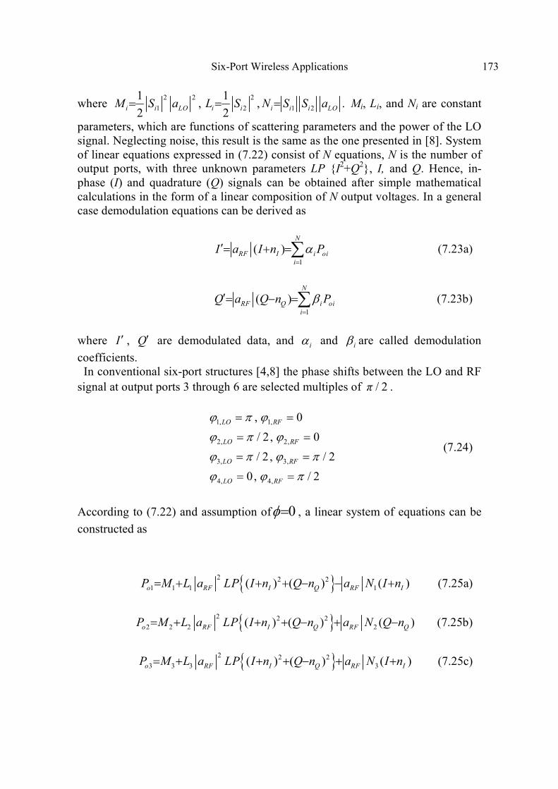
Six-Port Wireless Applications 173
where2 2 2
1 2 1 2
1 1, , .
2 2i i LO i i i i i LOM S a L S N S S a= = = Mi, Li, and Ni are constant
parameters, which are functions of scattering parameters and the power of the LO
signal. Neglecting noise, this result is the same as the one presented in [8]. System
of linear equations expressed in (7.22) consist of N equations, N is the number of
output ports, with three unknown parameters LP I2+Q2
, I, and Q. Hence, in-
phase (I) and quadrature (Q) signals can be obtained after simple mathematical
calculations in the form of a linear composition of N output voltages. In a general
case demodulation equations can be derived as
1
( )N
RF I i oii
I a I n Pα=
′= + =∑ (7.23a)
1
( )N
RF Q i oii
Q a Q n Pβ=
′= − =∑ (7.23b)
where I ′ , Q′ are demodulated data, and iα and iβ are called demodulation
coefficients.
In conventional six-port structures [4,8] the phase shifts between the LO and RF
signal at output ports 3 through 6 are selected multiples of / 2π .
1, 1,
2, 2,
3, 3,
4, 4,
, 0
/ 2, 0
/ 2 , / 2
0, / 2
LO RF
LO RF
LO RF
LO RF
ϕ π ϕ
ϕ π ϕ
ϕ π ϕ π
ϕ ϕ π
= =
= =
= =
= =
(7.24)
According to (7.22) and assumption of 0φ= , a linear system of equations can be
constructed as
2 2 2
1 1 1 1( ) ( ) ( )o RF I Q RF IP M L a LP I n Q n a N I n= + + + − − + (7.25a)
2 2 2
2 2 2 2( ) ( ) ( )o RF I Q RF QP M L a LP I n Q n a N Q n= + + + − + − (7.25b)
2 2 2
3 3 3 3( ) ( ) ( )o RF I Q RF IP M L a LP I n Q n a N I n= + + + − + + (7.25c)

174 The Six-Port Technique with Microwave and Wireless Applications
2 2 2
4 4 4 4( ) ( ) ( )o RF I Q RF QP M L a LP I n Q n a N Q n= + + + − − − (7.25d)
where ,i iM L are defined in (7.22). For a general structure, I and Q can be
obtained using the above equations by a simple matrix calculation called the
demodulation process. Finally, demodulated data can be written as a linear
composition of known parameters, oiP .
1 1 4 2 3 3 4 4( )RF I o o o oI a I n P P P Pα α α α′= + = + + +
(7.26a)
1 1 2 2 3 3 4 4( )RF Q o o o oQ a Q n P P P Pβ β β β′= − = + + + (7.26b)
The above demodulation equations are simplified for symmetrical structure. For a
symmetrical structure, we can write
, , , 1, 2,3, 4i j i j i jM M L L N N i j= = = =
(7.27)
Hence, 3 1 2 4 1
1/(2 )N=− = =− =α α β β , 2 4 1 3
0= = = =α α β β , and demodulation equations
are in a simplest form as:
3 1 1( )/(2 )o oI P P N′= −
(7.28a)
2 4 1( )/(2 )o oQ P P N′= −
(7.28b)
Using additional ADCs and DSP units, these demodulation equations can be
implemented with accurate results. A low-cost implementation of (7.28) is the
conventional op-amp circuits [9], although the accuracy may be slightly reduced.
The system of linear equations in (7.25) has four equations and three unknown
parameters, so there is a dependent equation that can be eliminated. One way to
reduce the receiver’s cost and complexity is to eliminate one of the outputs, which
eliminates one power detector and one ADC. For example, by the elimination of
4oP , the demodulation equations can be rewritten as
3 1 1( )/(2 )o oI P P N′= −
(7.29a)
2 3 1 1[2 ( )]/(2 )o o oQ P P P N′= − +
(7.29b)

Six-Port Wireless Applications 175
These equations convert six-port structure to five-port structure. For cost
reduction, we can implement these equations by an electronic circuit which can be
realized using conventional operational amplifiers as shown in Figure 7.6. In this
circuit we use variable resistors to remove the unwanted constant DC components.
The calibration process can be done by varying the value of the resistors in
horizontal arms. Moreover, there are various I/Q generation algorithms that may
be used for six-port and five-port receivers [10–12].
Beside the noise, in the case of nonideal phase shift, additional terms appeared in
(7.25) as
2 2 2( ) ( )
( ) ( ), 1,2,3, 4
oi i i RF I Q
RF i i I RF i i Q
P M L a LP I n Q n
a C N I n a S N Q n i
= + + + −
+ + + − = (7.30)
where ( )cosi iC φ ϕ= − and ( )sini iS φ ϕ= − are constants for a six-port architecture
with specific phase deviations.
Figure 7.6 Baseband circuit for a five-port structure (I/Q calculation block). (© 2009 IET [16].)
Therefore, a combination of at least three outputs is required in demodulation
process, and in this general case, the demodulation equation is rewritten as
1 1 2 2 3 3( )RF I o o oI a I n P P Pα α α′= + = + + (7.31a)
1 1 2 2 3 3( )RF Q o o oQ a Q n P P Pβ β β′= − = + +
(7.31b)

176 The Six-Port Technique with Microwave and Wireless Applications
which can be implemented by a simple modification in an electronic circuit of IQ
calculation.
7.2.3 Six-Port Receiver Calibration
To have an optimal receiver, the demodulation coefficients must be found for each
carrier frequency to minimize BER. Here, a calibration method is described based
on S-parameters of multiport linear structure as well as the characteristics of
nonlinear power detectors. The S-parameters of structures can be obtained from
simulation or measurement. At first stage, the output powers are calculated for
each constellation points using S-parameters and the characteristics of power
detectors. The calibration is performed using the video signals. Accordingly, for
each constellation point, I, Q, and oiP are known. Considering M as constellation
points ( M N≥ ), a system of linear equations B=A.X must be solved for
demodulation purpose. The matrices A and X are as follows:
11 12 1 11 22 1
21 22 2 21 22 2
1 2 1 2
1
4
|
|
,|
|
|
o o o N o o o N
o o o N o o o N
oM oM oMN oM oM oMN
N
P P P P P P
P P P P P PA
P P P P P P
X
αα
α
=
=
⋯ ⋯
⋯ ⋯
⋮ ⋮ ⋱ ⋮ ⋮ ⋮ ⋱ ⋮
⋯ ⋯
⋮
1
2
1
4
and
M
N
I
I
I
B
ββ
β
=
⋮
⋮
1
2
M
Q
Q
Q
⋮
(7.32)
The system must be solved to obtain demodulation coefficients iα and iβ . For
a five-port receiver, this system of equations is simplified to match the one
presented earlier in [13]. As may be seen, the number of equations is greater than
unknown parameters. Accordingly, a least squares solution must be implemented
to find the unknown coefficients. Therefore, a calibration procedure to solve the
least squares solution X that minimizes the norm of B-A*X is required. This
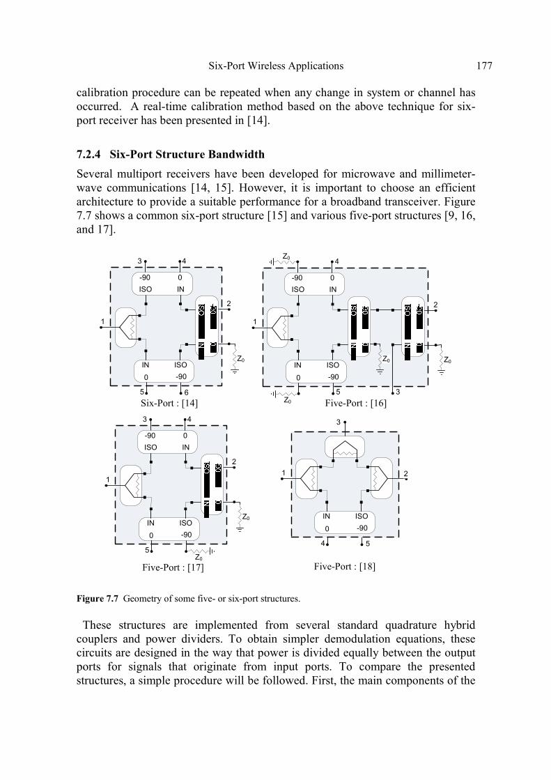
Six-Port Wireless Applications 177
calibration procedure can be repeated when any change in system or channel has
occurred. A real-time calibration method based on the above technique for six-
port receiver has been presented in [14].
7.2.4 Six-Port Structure Bandwidth
Several multiport receivers have been developed for microwave and millimeter-
wave communications [14, 15]. However, it is important to choose an efficient
architecture to provide a suitable performance for a broadband transceiver. Figure
7.7 shows a common six-port structure [15] and various five-port structures [9, 16,
and 17].
-90 0
ISO IN
-90
0
ISOIN
1
3 4
5 6
2
Z0
-90 0
ISO IN
-90
0
ISOIN
1
3 4
5
2
Z0
Z0
-90 0
ISO IN
-90
0
ISOIN
1
3
4
5
Z0
Z0
Z0
2
Z0
4
3
5
Six-Port : [14] Five-Port : [16]
Five-Port : [17] Five-Port : [18]
-90
0
ISOIN
1 2
Figure 7.7 Geometry of some five- or six-port structures.
These structures are implemented from several standard quadrature hybrid
couplers and power dividers. To obtain simpler demodulation equations, these
circuits are designed in the way that power is divided equally between the output
ports for signals that originate from input ports. To compare the presented
structures, a simple procedure will be followed. First, the main components of the

178 The Six-Port Technique with Microwave and Wireless Applications
multiport structures are designed in a desired frequency 0f (4.5 GHz is selected in
this work) and implemented with transmission lines to obtain complete structure.
Then the S-parameter of each structure is obtained from RF simulations.
Using these parameters and the characteristics of power detectors, the output
powers are calculated for each constellation point (specific I and Q ) in a QAM
modulation scheme. By known values of I , Q , and oiP , the linear system of
equations in (7.2) can be solved to obtain the demodulation coefficients iα and
iβ . Then, the circuit is investigated in the different frequencies and the average of
error vector magnitudes (EVM) in QAM constellation points are calculated for
various structures. The EVM is calculated using
2 2
2 2
( ) ( )I I Q QEVM
I Q
′ ′− + −=
+
(7.33)
where I ′ and Q′ are demodulated values which are calculated by (7.2), using the
demodulation coefficients from the previous step and output powers for I and
Q in new operational frequencies.
Figure 7.8 shows an average EVM for various structures in a frequency band of
0.8 0f to 1.2 0f . The demodulation coefficients have been calculated for0f . As
may be seen, the EVM for all structures is equal to the expected value of zero at
0f . As may be seen, the smaller and larger bandwidths are obtained from five-
port structures presented in [9] and [17], respectively. The six-port circuit of [15]
supports a smaller bandwidth than the five-port circuit of [17].
7.3 SIX-PORT IN SOFTWARE RADIO APPLICATIONS
Due to various wireless communication standards, achieving a multi-mode and
multistandard receiver is desirable. Such receivers must satisfy the requirements
to have broadband or multi-band RF stages, to have low cost, size, and power
consumption, and to be compatible with the digital signal processing section. In
order to obtain these properties, the RF stage architecture must be chosen
properly. It is obvious that the conventional superheterodyne architectures are not
suitable solutions for satisfying these requirements because they require to several
image rejection filters to eliminate image responses [18].
Moreover, when the receiver switches to another standard, it needs to use a new
image rejection filter. This problem can be solved by direct conversion
architectures because they have no image response, and thus do not require any
image rejection filters. In addition, the direct conversion architectures have more
integrated size and lower power consumption than the superheterodyne ones [18].

Six-Port Wireless Applications 179
0.8 fo 0.9 fo fo 1.1 fo 1.2 fo0
0.1
0.2
0.3
0.4
0.5
0.6
0.7
frequency
EVM
Ref. [18]
Ref. [17]
Ref. [16]
Ref. [14]
Figure 7.8 Average EVM for various multiport structures.
Software defined radio is the main architecture for future advanced radio systems
[19]. A software defined radio (SDR) is a radio in which the operating
parameters,including the frequency range, modulation type, and maximum
radiated or conducted output power can be altered by making a change in the
software without making any hardware changes [20]. The advantages of six-port
architecture such as compatibility with DSP, ultra low power consumption, and
broadband specifications make it very suitable for software defined radio
applications. Figure 7.9(a) shows the structure of a six-port SDR receiver [20, 21].
The RF front-end consists of a low-noise amplifier (LNA), a BPF, a six-port
junction, and four power detectors. The six-port junction works as an RF
downconverter in the proposed receiver. Port 2 connects to the RF signal and port
1 connects to the local oscillator (LO); the other four ports are connected to RF
power detectors. The output voltages of the RF power detectors represent power
levels of the four output ports of the six-port circuit. Signals from ports 1 and 2
are directly downconverted from RF to baseband frequency in the form of the

180 The Six-Port Technique with Microwave and Wireless Applications
output of power detectors. The signals from power detectors are then sent to the
DSP section after passing a set of BPFs and baseband amplifiers.
The DSP section is responsible for the baseband signal processing such as
demodulation and decoding. The receiver is designed to operate at the microwave
frequency and operates over a wideband for multimode schemes. For an SDR
receiver platform, the DSP computation algorithms and calibration methods are
crucial.
(a)
(b)
Figure 7.9 (a) Architecture of six-port software receiver. (b) Six-port receiver algorithm.
Figure 7.9(b) shows the algorithm flowchart of the SDR six-port receiver [21].
Subsequent to the data acquired from the antenna, some samples are selected for
calibration. This six-port calibration provides the coefficients needed for
computation to calculate the in-phase and quadrature (I/Q) data. Following a
decision algorithm, the signals are then demodulated. This process is a universal
demodulation algorithm for six-port receivers. A calibration method free from any
external connection must be used. In this receiver platform, a real-time six-port
calibration method [14] is adopted and the demodulation results for different
modulation schemes are analyzed.
7.3.1 Five-Port Structure in Software Defined Radio Applications
The performance of the five-port structure has been studied as a software radio
receiver as well [4]. The center frequency was considered to be 2.4 GHz, and the
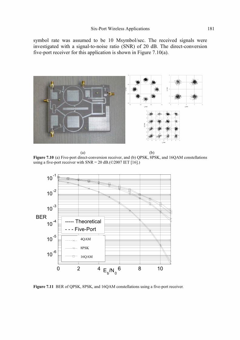
Six-Port Wireless Applications 181
symbol rate was assumed to be 10 Msymbol/sec. The received signals were
investigated with a signal-to-noise ratio (SNR) of 20 dB. The direct-conversion
five-port receiver for this application is shown in Figure 7.10(a).
(a) (b)
Figure 7.10 (a) Five-port direct-conversion receiver, and (b) QPSK, 8PSK, and 16QAM constellations
using a five-port receiver with SNR = 20 dB.(©2007 IET [16].)
Figure 7.11 BER of QPSK, 8PSK, and 16QAM constellations using a five-port receiver.
0 2 4 6 8 10
10-6
10-5
10-4
10-3
10-2
10-1
Eb /N0
4QAM
8QAM
16QAM
----- Theoretical
- - - Five-Port
4QAM
8PSK
16QAM
BER

182 The Six-Port Technique with Microwave and Wireless Applications
The constellation diagrams for various modulation schemes (QPSK, 8PSK, and
16QAM) using the five-port receiver are shown in Figure 7.10(b). The results
imply that it is possible to implement the five-port circuit precisely in MQAM and
MPSK demodulators, and it can be used as a direct demodulator receiver.
Theoretical and simulated BERs versus Eb/N0 for different modulation schemes
(QPSK, 8PSK, and 16QAM) are illustrated in Figure 7.11.
7.4 SIX-PORT IN UWB APPLICATIONS
The recent allowance of frequencies between 3 GHz and 10 GHz for UWB
applications would allow higher data throughput up to 500 Mbps over short
distances [22]. Apart from high data rates, the other compelling features of UWB
would be potentially lower cost and higher levels of integration. Ideal targets for
UWB systems are low power, low cost, high data rates, precise positioning
capability, and extremely low interference [22, 23]. The common choices of the
modulation scheme in UWB communication are pulse position modulation
(PPM), pulse amplitude modulation (PAM), and pulse shape modulation (PSM)
[24]. The long-term vision for UWB is a low power high-speed standard that
provides wireless connectivity for battery operated devices.
Pulse-based systems are one approach for implementing UWB systems to use the
UWB bands. A pulse-based system may use a modulated pulse to transfer
information. Such systems require RF front-end to support a wideband signal.
Therefore, a conventional design technique as well as RF front-end architecture
for narrowband applications must be modified and improved to overcome
obstacles in implementing RF front-end for emerging wideband applications.
Because of the characteristics of the pulse, the RF front-end of such systems tends
to be simple, using direct conversion methods. However, processing these
extremely wideband signals using an ADC would be quite challenging.
It is important to choose an efficient architecture to provide the suitable
performance for a UWB transceiver. The six-port structure is implemented for
UWB [18]. This receiver and transmitter architecture uses six-port circuits to
digitally modulate and demodulate a full 1-GHz phase spectrum. The six-port
impulse radio block diagram is shown in Figure 7.12. Differences between six-
port impulse radios and other UWB radios are in the modulation and
demodulation schemes including related radio hardware/software/signal
processing. It consists of a wideband six-port circuit, a switch matrix, and open
and short terminations.
Each component has wideband characteristics. The impulse radio hardware and
software for direct modulation and demodulation are experimentally investigated
for UWB applications [18]. The radio demonstration platform contained two six-
port interferrometers (one for modulation and the other for demodulation), four-
channel digital signal processors, four single-pole double throw (SPDT) switches,
two antennas (Rx/Tx), and various minor components such as wideband short and

Six-Port Wireless Applications 183
open circuit terminations. The radio is designed to operate in wideband channels
(over 500 MHz per channel) as required in UWB communication systems.
7.4.1 Six-Port Impulse Radio Modulator
Figure 7.12 shows the six-port impulse radio modulator. The modulator operates
as follows: port 1 is fed with a pulse signal, which is routed to ports 3–6 through
the different branches of the six-port circuit.
Figure 7.12 The six-port impulse radio test block diagram.( © 2008 IEEE [18].)

184 The Six-Port Technique with Microwave and Wireless Applications
(a)
(b) Figure 7.13 (a) Six-port impulse radio QPSK modulator measurements and simulations from 3 GHz to 4 GHz. (b) Demodulator test results showing normalized output voltages of detectors versus phase
difference between two input signals taken at any frequency within the operating channel (3 GHz to 4
GHz).(© 2008 IEEE [18].)
Signals present at ports 3–6 are routed to different terminations by the switch
matrix, which is controlled by baseband data. Port 2 outputs the digitally
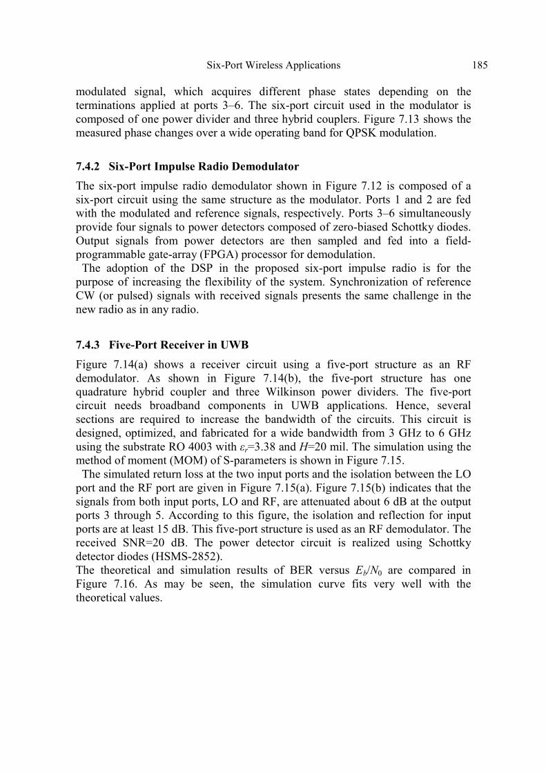
Six-Port Wireless Applications 185
modulated signal, which acquires different phase states depending on the
terminations applied at ports 3–6. The six-port circuit used in the modulator is
composed of one power divider and three hybrid couplers. Figure 7.13 shows the
measured phase changes over a wide operating band for QPSK modulation.
7.4.2 Six-Port Impulse Radio Demodulator
The six-port impulse radio demodulator shown in Figure 7.12 is composed of a
six-port circuit using the same structure as the modulator. Ports 1 and 2 are fed
with the modulated and reference signals, respectively. Ports 3–6 simultaneously
provide four signals to power detectors composed of zero-biased Schottky diodes.
Output signals from power detectors are then sampled and fed into a field-
programmable gate-array (FPGA) processor for demodulation.
The adoption of the DSP in the proposed six-port impulse radio is for the
purpose of increasing the flexibility of the system. Synchronization of reference
CW (or pulsed) signals with received signals presents the same challenge in the
new radio as in any radio.
7.4.3 Five-Port Receiver in UWB
Figure 7.14(a) shows a receiver circuit using a five-port structure as an RF
demodulator. As shown in Figure 7.14(b), the five-port structure has one
quadrature hybrid coupler and three Wilkinson power dividers. The five-port
circuit needs broadband components in UWB applications. Hence, several
sections are required to increase the bandwidth of the circuits. This circuit is
designed, optimized, and fabricated for a wide bandwidth from 3 GHz to 6 GHz
using the substrate RO 4003 with εr=3.38 and H=20 mil. The simulation using the
method of moment (MOM) of S-parameters is shown in Figure 7.15.
The simulated return loss at the two input ports and the isolation between the LO
port and the RF port are given in Figure 7.15(a). Figure 7.15(b) indicates that the
signals from both input ports, LO and RF, are attenuated about 6 dB at the output
ports 3 through 5. According to this figure, the isolation and reflection for input
ports are at least 15 dB. This five-port structure is used as an RF demodulator. The
received SNR=20 dB. The power detector circuit is realized using Schottky
detector diodes (HSMS-2852).
The theoretical and simulation results of BER versus Eb/N0 are compared in
Figure 7.16. As may be seen, the simulation curve fits very well with the
theoretical values.

186 The Six-Port Technique with Microwave and Wireless Applications
LP
F
Pow
er
Dete
cto
r
P1
P2
P3
(a)
(b)
Figure 7.14 A five-port UWB receiver. (a) Functional block diagram. (b) The microstrip layout.
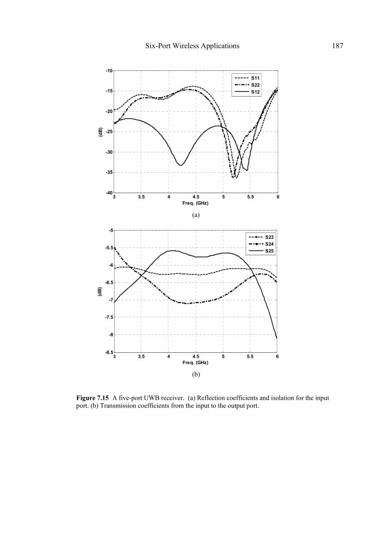
Six-Port Wireless Applications 187
3 3.5 4 4.5 5 5.5 6-40
-35
-30
-25
-20
-15
-10
Freq. (GHz)
(dB)
S11
S22
S12
(a)
3 3.5 4 4.5 5 5.5 6-8.5
-8
-7.5
-7
-6.5
-6
-5.5
-5
Freq. (GHz)
(dB)
S23
S24
S25
(b)
Figure 7.15 A five-port UWB receiver. (a) Reflection coefficients and isolation for the input
port. (b) Transmission coefficients from the input to the output port.
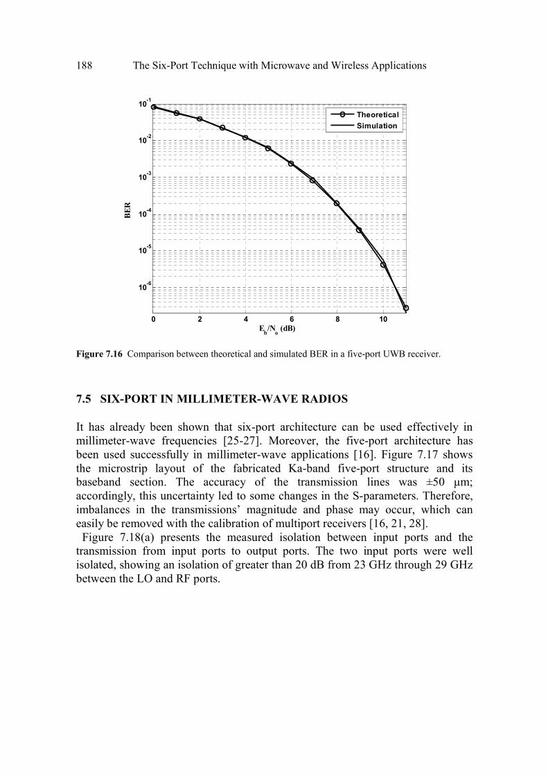
188 The Six-Port Technique with Microwave and Wireless Applications
0 2 4 6 8 10
10-6
10-5
10-4
10-3
10-2
10-1
Eb/N
o (dB)
BE
R
Theoretical
Simulation
Figure 7.16 Comparison between theoretical and simulated BER in a five-port UWB receiver.
7.5 SIX-PORT IN MILLIMETER-WAVE RADIOS
It has already been shown that six-port architecture can be used effectively in
millimeter-wave frequencies [25-27]. Moreover, the five-port architecture has
been used successfully in millimeter-wave applications [16]. Figure 7.17 shows
the microstrip layout of the fabricated Ka-band five-port structure and its
baseband section. The accuracy of the transmission lines was ±50 µm;
accordingly, this uncertainty led to some changes in the S-parameters. Therefore,
imbalances in the transmissions’ magnitude and phase may occur, which can
easily be removed with the calibration of multiport receivers [16, 21, 28].
Figure 7.18(a) presents the measured isolation between input ports and the
transmission from input ports to output ports. The two input ports were well
isolated, showing an isolation of greater than 20 dB from 23 GHz through 29 GHz
between the LO and RF ports.

Six-Port Wireless Applications 189
Figure 7.17 A Ka-band receiver fabricated using a microstrip line. (© 2009 IET [16].)
These measurement results indicate an attenuation of approximately 10 dB.
Figure 7.18(b) also shows the absolute measured phase shift from the input ports
to ports 3 and 4. The desired 180° phase difference between RF signals at ports 3
and port 4 was achieved, and the LO signal had the same phase shift at two output
ports. Finally, the circuit was tested as a direct demodulator of a 2 Mbit/s QPSK
modulated signal.
The RF and LO input levels were set to -20 dBm at center frequency. The I and
Q signals were obtained using an electric circuit shown in Figure 7.18(c). Using
the XY display of the oscilloscope, the I/Q constellation can be achieved from
analog output signals, as shown. The demodulated QPSK signal confirmed the
accuracy of the five-port receiver in millimeter-wave applications.
A six-port transceiver has been implemented using CMOS technology in 60 GHz
[26]. The target is to provide a very low-cost, miniaturized, and low DC power
consumption transceiver for IEEE 802.15 applications. The transmitter is
composed of a reflection-type I/Q modulator and a buffer amplifier, while the
receiver consists of an LNA and a six-port demodulator.
An on-chip VCO provides the LO signals for the transmitter and receiver and an
SPDT switch is used to select the transmitting or receiving path. This block
diagram of the transceiver and its chip photo are shown in Figure 7.19. The total
DC power consumption of the transceiver is less than 100 mW.

190 The Six-Port Technique with Microwave and Wireless Applications
(a)
(b)
(c)
Figure 7.18 (a) The Ka-band receiver, (b) the measured values for transmission and isolation for the
Ka band five-port receiver, and (c) The constellation diagram for demodulated I and Q signals of
QPSK modulation.( © IET 2009 [16].)

Six-Port Wireless Applications 191
Figure 7.19 (a) Block diagram and (b) chip photo of the 60-GHz CMOS six-port transceiver. The transmitter is composed of a reflection-type I/Q modulator and a buffer amplifier while the receiver
consists of an LNA and a six-port demodulator. An on-chip VCO provides the LO signals for the
transmitter and receiver and an SPDT switch is used to select the transmitting or receiving path. (© 2009 IEEE [26].)
192 The Six-Port Technique with Microwave and Wireless Applications
7.6 COMPARISON BETWEEN SIX-PORT AND CONVENTIONAL
RECEIVERS
Six-port microwave receivers push the boundaries regarding price and the upper
frequency limit. To enable a serious validation of the six-port technology, we have
to benchmark it with existing receiver architectures [27]. This section compares
the six-port receiver with conventional receivers [27, 29].
7.6.1 RF Performance
Phase Accuracy
In a conventional receiver, the phase noise of the local oscillator (LO) will be
directly transformed to the phase noise in the baseband. This will lead to neighbor
channel interference, caused by reciprocal mixing, and therefore reduce the
selectivity of the receiver. In the six-port receiver, as in the direct conversion
receiver, additional phase inaccuracy will be introduced. Because of this
unavoidable phase imbalance, phase distortion can be generated. However, phase
distortion can be reduced by performing an accurate calibration.
Noise Figure
The noise figure is usually defined by the LNA in a receiver. If no LNA is used,
we have to compare the noise of a mixer to the noise of a power detector receiver.
For frequencies beyond 50 GHz, both are usually built up using Schottky diodes.
The noise figure for diode mixers is comparable to its conversion loss which is
typically about 7 dB. Simulations on microwave power detectors using a beam
lead GaAs Schottky diode have shown that the noise figure goes down to 4.8 dB
for input powers smaller than -20 dBm.
LO Power
For most mixers to obtain a good conversion gain, the power of the local oscillator
should be in the range of 0 to 10 dBm [30]. On the other hand, a suitable condition
for six-port receivers is an LO power in the area of the receiver input power which
is much lower in practical applications (less that -20 dBm).
In-Band Dynamic Range
For six-port receivers this dynamic range is mainly limited by the accuracy of the
calibration and the detector sensitivity. First trials have shown a dynamic range of
40 dB [31, 32]. Calibration will also limit the linearity of the receiver. For mixer-
based receivers the dynamic range is limited by the linearity. This results in a

Six-Port Wireless Applications 193
dynamic range of about 90 to 100 dB for a signal bandwidth of 10 MHz. The
dynamic range of the receiver can also be increased well above 70 dB with an
AGC inserted within the LNA [33].
Self Mixing Effects
Direct coupling and external reflections lead to a DC offset for a direct conversion
receiver and a six-port receiver. Direct conversion receivers usually contain some
signal processing unit to cope with this effect. It was recently shown that six-port
receivers are less sensitive to DC offset in comparison to subharmonically
pumped direct conversion receivers [29].
7.6.2 Boundary Limitations
Size
The size of mixer-based architectures is mainly given by active components and
filters. The usual setup of a six-port is about ¾ λ in square. For V-, W-, and
D-band applications it is very possible to integrate the six-port on a chip.
Cost
The cost of a direct conversion receiver depends very much on the frequency
range. Especially for frequencies in the W- and D-bands, mixers become rare and
expensive, whereas power detectors are available for higher frequencies. For
millimeter-wave signal generation usually a lower frequency LO is followed by a
frequency multiplier, which produces a small LO power. The six-port receiver
will have a cost advantage by reduced LO power requirements. In conclusion, six-port receivers are a suitable and cost-effective alternative to
existing mixer-based receiver architectures, especially in the millimeter-wave and
sub-millimeter-wave range. In this frequency range we usually do not have to
cope with strong neighbor channel interference, so the reduced dynamic range will
be acceptable. Moreover, it has recently been shown that the six-port receiver
architecture is less sensitive to LO power variations and phase errors than the
antiparallel diode receivers [29].
7.7 SIX-PORT IN PHASED-ARRAY SYSTEMS
Six-port junctions have been primarily used as reflectometers [34, 35], that is, to
measure the reflected-to-incident waves ratio at one port of the junction.
Alternatively, one can measure the complex ratio of incident waves at two
194 The Six-Port Technique with Microwave and Wireless Applications
different ports of the junction [36, 37]. In the case of a linear array, the array
factor can be fully determined if the signals radiated by the elements are related to
each other by complex ratios. These ratios depend on the feed network but also on
the coupling between the array elements. This is represented as a coupling
network box in Figure 7.20. Let us assume that all the active elements have the
same radiation pattern and that waves a1 and a2 are not reflected back to the
antenna. The goal herein is to determine the ratio a1/a2 from the power readings. If we can determine this ratio for all the element pairs of the array, it will be
possible to calculate the array factor. To illustrate the procedure, let us consider
the two-branch network of Figure 7.20 where waves a1 and a2 are absorbed by
matched terminations. Using the superposition of sources, we can write:
7 8, 1, 2, ,6i i ia M b N b i= + = …
(7.34)
From (7.34) with i = 1 and i = 2, we have:
7 1 2 2 1 1 2 1 2
8 1 1 1 2 1 2 1 2
( ) / ( )
( ) / ( )
b a N a N M N N M
b a M a M M N N M
= − −
= − −
Using these expressions for b and bs, (7.34) can be rewritten as
1 2, 3, ,6i i ia Pa Q a i= + = …
(7.35)
Equation (7.35) has the classic form of six-port relations [36]. It relates the
incident signals on the power detectors to the waves radiated by elements 1 and 2.
Using (7.35), it is easy to implement the calibration technique for six-port
reflectometers given in [18] or [38] by replacing the unknown reflection
coefficient (b2/a2) by the ratio of interest, namely a2/a1. The remaining difficulty is
the establishment of accurate a1/a2 ratios to be used as standards in the calibration.
In the case of an antenna array, the an values used in the calibration of the
junctions embedded between each pair of elements can be determined by
measuring the radiation pattern of the array. For an N-element linear array, we can
write the following expression for the θ-component of the radiated far-field
( , )E rθ in the XZ plane:
sin
1
( , ) ( )j r N
j ndn
n
eE r K a e
r
− ββ θ
=
θ = θ ∑ (7.36)

Six-Port Wireless Applications 195
a4
a5
a6
a3
Figure 7.20 Six-port in phased-array systems.
where ( )K θ includes all the constants and the array-element factor. ( )K θ can be
measured by feeding only one element of the array. When all the active elements
are fed simultaneously, we can measure ( , )E rθ for N different values of angle θ
and build a system of N linear equations. This system can then be solved to give
one set of ans. All the data necessary to calibrate the N-1 six-port junctions can be
obtained from four far-field pattern measurements [39]. In a phased array, we
arbitrarily choose four different settings of the phase shifters. For each setting,
both the phase and magnitude patterns of the array are measured and the [an]
vectors are determined by solving the linear system of equations. The power
readings of the six-port junctions are also recorded. This data can then be used to
calibrate each one of the junctions with the procedure given in [29]. Once the
junctions are calibrated, all the ai values can be related to each other for any state
of the feed network since the six-port measurements can be used to calculate the
ratio of each pair of adjacent signals. This allows a real-time determination of the
array factor [40, 41].

196 The Six-Port Technique with Microwave and Wireless Applications
References
[1] Zhao, Y., C. Viereck, J. F. Frigon, R. G. Bosisio, and K. Wu, “Direct Quadrature Phase Shift
Keying Modulator Using Six-Port Technology,” Electronics Letters, Vol. 41, No. 21, pp. 1180–
1181, October. 2005
[2] Lou, B., and M.Y. Chia, “Direct Quadrature 16QAM Six-Port Modulator,” Electronics Letters,
Vol. 44, No. 15, July 2008.
[3] Boulajfen, N., F. M. Ghannouchi, and A. B. Kouki, “A Homodyne Multiport Network Analyzer
for S-Parameter Measurements of Microwave N-port Circuits/Systems,” Microwave Opt. Technol. Lett., Vol. 24, No. 1, pp. 63–67, January 2000.
[4] Mohajer, M., A. Mohammadi, and A. Abdipour, “Direct Conversion Receivers Using Multi-Port Structures for Software Defined Radio Systems,” IET Microwaves, Antennas & Propagation, 2007, Vol. 1, No.2, pp. 363–372, April 2007.
[5] Tatu, S. O., K. Wu, and T. Denidni, “Multi-Band Multi-Port Direct Conversion Receiver:
Design, Implementation and Demodulation Results,” Microwave and Optical Technology Letter,
Vol. 48, No. 4, pp. 817–822, April 2006.
[6] Hoer, C. A., and K. C. Roe, “Using an Arbitrary Six-Port Junction to Measure Complex Voltage
Ratios,” IEEE Trans. Microwave Theory & Tech., Vol. MTT-23, pp. 978–984, December 1975.
[7] Mohajer, M., and A. Mohammadi, “A Novel Architecture for Six-Port Direct Conversion
Receiver,” IEEE PIMRC 2004, Vol .4, pp. 2705–2709, September 2004.
[8] Buracchini, E., “The Software Radio Concept,” IEEE Communication Magazine, Vol. 38, pp.
138–143, September 2000.
[9] Mohajer, M., A. Mohammadi, and A. Abdipour, “A Software Defined Radio Direct Conversion
Receiver,” European Microwave Conference, EUMC 2005, Vol. 3, pp. 1823–1826, 2005.
[10] Huang, X., D., Hindson, M., de Leseleuc, and M., Caron., “I/Q-Channel Regeneration in 5-Port
Junction Based Direct Receivers,” IEEE MTT-S 1999, pp. 169–173, February 21-24, 1999.
[11] Cho, Y. H., B. W. Kim, and D. J. Park, “ I/Q Regeneration Algorithm for Direct Conversion
Receiver Using 5-Port Junction,” 2006 8th International Conference on Signal Processing,
November 2006.
[12] Hentschel, T., “A Simple IQ-Regeneration Technique for Six-Port Communication Receivers,”
First International Symposium on Control, Communications and Signal Processing, pp. 311–
314, 2004.
[13] Neveux, G., B. Huyart, and G. J. Rodriguez-Guisantes, “Wide-Band RF Receiver Using the Five-
Port Technology,” IEEE Transactions on Vehicular Technology, Vol. 53, No. 5, September 2004.
[14] Y. Xu, and R. G. Bosisio, “On the Real-Time Calibration of Six-Port Receivers (SPRs),”
Microwave and Optical Technology Letters, Vol. 20, No. 5, March 5, 1999.
[15] Zhao, Y., J .F. Frigon, K. Wu, and R. G. Bosisio, “Multi(Six)-Port Impulse Radio for Ultra-
Wideband,” IEEE Trans. Microwave Theory & Tech., Vol. 54, No. 4, June 2006, pp. 1707–
1712.
[16] Mirzavand, R., A. Mohammadi, and A. Abdipour, “Low-cost Implementation of Broadband
Microwave Receiver in Ka Band Using Multi-Port Structures,” IET Microwaves, Antennas & Propagation, Vol. 3, No. 3, pp. 483–491, 2009 .

Six-Port Wireless Applications 197
[17] Mirzavand, R., A. Mohammadi, and A. Abdipour, “Five-Port Transceiver for WiMAX
Applications,” 17th International Conference on Microwaves, Radar and Wireless Communications MIKON, Wroclaw, Poland, pp. 19–21 May 2008.
[18] Bosisio, R. G., Y. Y. Zhao, X. Y. Xu, S. Abielmona, E. Moldovan, Y. S. Xu, M. Bozzi, S. O.
Tatu, J. F. Frigon, C. Caloz, and K. Wu, “New-Wave Radio,” IEEE Microwave Magazine, pp.
89–100, February 2008.
[19] Ghannouchi, F. M., “Software Defined Radio Transmitters for Advanced Wireless and Satellite
Communications Systems,” Microwave Journal, Vol. 51, No. 5, pp. 202–216, May 2008.
[20] Chang, K., Encyclopedia of RF and Microwave Engineering, New York: Wiley, 2005.
[21] Xu, X., R. G. Bosisio, and K. Wu, “Analysis and Implementation of Six-Port Software-Defined
Radio Receiver Platform,” IEEE Trans. Microwave Theory & Tech., Vol. 54, No. 7, 2006, pp.
2937–2943.
[22] Yang, L., and G.B. Giannakis, “Ultra-Wideband Communications: an Idea Whose Time Has
Come,” IEEE Signal Processing Magazine, Vol. 21, No. 6, pp. 26–54, November 2004.
[23] Bellorado, J., S. S. Ghassemzadeh, L. J. Greenstein, T. Sveinsson, and V. Tarokh, “Coexistence
of Ultra-Wideband Systems with IEEE 802-11a Wireless LANs,” IEEE Global Telecommunications Conference, Vol. 1, pp. 410–414, December 2003.
[24] Da Silva, J. A. N., and M. L. R. de Campos, “Performance Comparison of Binary and Quaternary
UWB Modulation Schemes,” Proc. IEEE GLOBECOM Conf., San Francisco, CA, 2003, pp.
789–793.
[25] Li, J., R. G. Bosisio, and K. Wu, “Computer and Measurement Simulation of a New Digital
Receiver Operating Directly at Millimeter Wave Frequencies,” IEEE Trans. Microwave Theory Tech., Vol. 43, No. 12, pp. 2766–2772, December 1995..
[26] Wang, H., K. Lin, Z. Tsai, L. Lu, H. Lu, C. Wang, J. Tsai, T. Huang, and Y. Lin, “MMICs in the
Millimeter-Wave Regime,” IEEE Microwave Magazine, pp. 99–117, February 2009.
[27] Eireiner, T., and T. Müller, “Six-Port Receiver for mm-Wave – Concept, Evaluation and
Implementation,” IEEE MELECON 2006, Benalmádena (Málaga), Spain, May 16-19, 2006.
[28] Ghannouchi, F. M., and R. G. Bosisio, “An Alternative Explicit Six Port Matrix Calibration
Formalism Using Five Standards,” IEEE Trans. MTT, Vol. 36, No. 3, pp. 494–498, 1988.
[29] Khaddaj Mallat, N., E. Moldovan, and S. O. Tatu, “Comparative Demodulation Results for Six-
Port and Conventional 60 GHz Direct Conversion Receivers,” Progress in Electromagnetics Research, PIER, Vol. 84, pp. 437–449, 2008.
[30] Hewlett Packard, “The Schottky Diode Mixer,” Application Note 995.
[31] Jürgensen, J.-U., D. Krupezevic, M. Ratni, and Z. Wang, “Baseband Aspects of a Direct
Conversion Receiver Concept Using Five-Port Technology,” 2nd Karlsruhe Workshop on Software Radio, Karlsruhe, March 2002.
[32] Demers, Y., R. G. Bosisio, and F. M. Ghannouchi, “Repetitive and Single Shot Pulse Microwave
Six-Port Reflectometer,” IEEE Trans. on Instrument and Measurement, No.1. February 1990.
[33] Tatu, S. O., E. Moldovan, K. Wu, and R. G. Bosisio, “A New Direct Millimeter-Wave Six-Port
Receiver,” IEEE Trans. Microwave Theory & Tech., Vol. 49, No.12, pp. 2517–2524, December
2001.
[34] Engen, G. F., “The Six-Port Reflectometer: an Alternative Network Analyzer,” IEEE Trans. Microwave Theory Tech., Vol. MTT-25, pp. 1075–1080, December 1977.

198 The Six-Port Technique with Microwave and Wireless Applications
[35] Engen, G. F., “An Improved Circuit for Implementing the Six-Port Technique of Microwave Measurements,” IEEE Trans. Microwave Theory Tech., Vol. MTI-25, pp. 1080–1083, December
1977.
[36] Cronson, H. M., “A Six-Port Automatic Network Analyzer,” IEEE Trans. Microwave Theory Tech., Vol. MTT-25, pp. 1086–1091, December 1977.
[37] Kamarei, M., “Vector Voltmeter Applications for Microwave Imaging,” Microwave Journal, Vol.
34, pp. 102–114, November 1991.
[38] Hodgetts, T. E., and E. J. Griffin, “A Unified Treatment of the Theory of Six-Port Reflectometer
Using the Minimum of Standards,” Tech. Report 83003, Royal Signals and Radar Establishment, Malvern, U.K., 1983.
[39] Laurin, J-J., R. G. Bosisio, F. M. Ghannouchi, “Calibration of a Monitoring System for Antenna
Arrays Based on Six-port Junctions,” 1992 IEEE Antennas and Propagation International Symposium, Chicago, IL, pp. 458–461, 1992.
[40] Cassivi, Y., F. M. Ghannouchi, and R. G. Bosisio, “Six-Port Junctions in a Phased Array Antenna
for Accurate Beam Steering,” 1992 IEEE Antennas and Propagation International Symposium, Chicago, IL, pp. 462–466, 1992.
[41] Ghannouchi, F. M., A. B. Kouki, and A. Khebir, “On the Experimental Characterization of
Electromagnetic Emissions from Printed Circuit Board,” 1993 IEEE AP-S International Symposium, Ann Arbor, MI, pp. 1490–1493, 1993.

199
Chapter 8
Six-Port Microwave Applications
The six-port architecture has found many applications in microwave systems.
These applications include reflectometer, directional finder, radar, antenna
measurement, and material characterization. Moreover, there have recently been
some applications using the six-port architecture in optical systems. In this
chapter, we present the theoretical issues and implementation techniques for using
the six-port in different microwave systems.
8.1 SIX-PORT MICROWAVE REFLECTOMETER
The six-port junction is commonly used as a reflectometer. Moreover, it can be
used in very high power microwave applications by the use of a hybrid directional
coupler.
8.1.1 Six-Port Reflectometer
The schematic of a six-port reflectometer for measuring the complex reflection
coefficient of a load (DUT) is shown in Figure 8.1. The setup is comprised of a
fixed frequency sinusoidal source, the passive six-port junction, and four power
meters. As discussed in previous chapters, the six-port theory establishes that the
complex reflection coefficient of the load, at frequency f0, can be precisely
determined, after calibration, from the four readings of the power meters.
In addition, if measurement in a certain frequency range is needed, the frequency
of the source would have to be changed. For any linear passive six-port junction,
as in Figure 8.1, the incident waves on the four power meters can be calculated as
[1]

200 The Six-Port Technique with Microwave and Wireless Applications
3 2 3 2R a T b+
4 2 4 2R a T b+
5 2 5 2R a T b+
6 2 6 2R a T b+
1a
1b
2a
2b2
2
L
a
bΓ =
1
2
3
4
5
6
Figure 8.1 Six-port reflectometer for complex reflection coefficient measurement.
2 2 3,4,5,6i i ib R a T b i= + =
(8.1)
where iR and iT are complex constants that only depend on the six-port junction
and the reflection coefficients of the power. Thus, the input to any of the power
meters is a linear combination of the incident b2 and reflected a2 wave on the DUT
with relative amplitude and phase given by the complex ratio
3, 4,5,6ii
i
Rq i
T= − = (8.2)
The power meter readings can then be calculated as
2 2
2 2
2
(1 )
1 3, 4,5,6
i i i
i i i L
P b
P b K q i
= − Γ
= − Γ = (8.3)
where iΓ are the reflection coefficients of the power meters and iK are real
constants defined as2 2
(1 )i i iK T= − Γ . Normalizing power (8.3) with respect to
the power of the reference port (e.g., P3, we come up with the three power ratio
equations)

Six-Port Microwave Applications 201
2
44 4
2
3 3 3
1
1
L
L
qP K
P K q
− Γ=
− Γ (8.4a)
2
55 5
2
3 3 3
1
1
L
L
qP K
P K q
− Γ=
− Γ
(8.4b)
2
66 6
2
3 3 3
1
1
L
L
qP K
P K q
− Γ=
− Γ (8.4c)
which are used to calculate the reflection coefficient of the load LΓ . In these
equations, there are four complex constants (q3, q4, q5, and q6) and three real
constants (the ratios 5 64
3 3 3
, ,K KK
K K K ), which depend on the six-port junction and
the reflection coefficient of the power meters but not on the load. These constants
are determined by calibration, that is, by measuring a certain number of known
loads (calibration standards).
As discussed in Chapter 5, there are procedures to calibrate the six-port by means
of a two-step procedure consisting of (1) a six-to-four port reduction, which
requires a certain number of different loads whose values do not need to be
exactly known, and (2) a classical one-port calibration that usually requires three
well-known standards (for example, load–short–open). However, any other set of
known loads can be used to calibrate the six-port.
Equation (8.4) defines three circles in the complex plane whose intersection is
the reflection coefficient of the load LΓ . The design criterion of the six-port
junction aims at making these equations as robust as possible. The port 3 may be
used as a reference of the DUT’s incident power (choosing 3 30 0R q= → = ) and
one may set the remaining measurement ports q4, q5, and q6 in a symmetrical
arrangement and located at 120 degree over a circumference of a radius equal to
1.5 [2].
Notice that with these design values, (8.4) represents three circles with fixed
centers, whose radii are directly proportional to the square root of the normalized
power measurements. In this case, the six-port operation is especially simple and
geometrically interpretable.

202 The Six-Port Technique with Microwave and Wireless Applications
8.2.1 High Power Microwave Reflectometer
In high power microwave radiation, the load characteristics may change with time
as its temperature increases. This change may result in an unmatched loading
condition between the power generator and the energy applicator. Moreover, in
practical microwave power applications such as microwave drying, it is often
desirable to monitor the power absorbed by the load.
A high power reflectometer is shown in Figure 8.2. It is composed mainly of a
low power microstrip six-port junction, a directional coupler, and a rectangular
waveguide section [2]. The key component of the high power reflectometer is the
hybrid waveguide to coaxial directional coupler used to reduce the power
exchange level and feed the lowpower six-port junction.
The measurement results of a given load for different input power are presented
in Table 8.1. As may be seen, the load reflection coefficient changes as the input
power varies. This technique can be efficiently used in thermo-dielectric
measurement applications [2].
12
3 4 5 6
Figure 8.2 Setup of a high power six-port reflectometer. (© 1995 IEEE [2].)

Six-Port Microwave Applications 203
Table 8.1
Measurement Results of a Given Load for Different Input Power
Input Power (watt) Reflection Coefficient (Γ)
200 00.234 129.07∠
50 00.237 128.50∠
12.5 00.239 129.13∠
3.13 00.245 131.27∠
8.2 SIX-PORT WAVE-CORRELATOR
8.2.1 General Concept
The schematic of a two-channel wave receiver using a six-port junction is shown
in Figure 8.3. The vector relation of two microwave signals a1 and a2, applied at
ports P1 and P2, is obtained by measuring the power levels at the four remaining
ports. The signal at port 1 usually comes from the reference generator and the one
at port 2 is unknown. The waves at the power detectors can be written as a linear
combination of the incident signals
1 2 3, 4,5,6i i ib A a B a i= + =
(8.5)
The power measured by the detectors can be expressed as the following values:
2 2 2 2
11i i i iP b A a t W= = + (8.6)
where ii
i
Bt
A= and W is the complex correlation ratio of the two incident waves a1
and a2, that is, 2
1
aW
a= . We denote an arbitrary side arm port by subscript h and
one of the other three by I; then the power ratio can be expressed as
2
, ,
1, 3,4,5,6;
1
i ii h i h
h h
P t WP T i h i h
P t W
+= = = ≠
+ (8.7)

204 The Six-Port Technique with Microwave and Wireless Applications
Linear
Passive
Six-port
Junction
P3
P4
P5
P6
3b
4b
5b
6b
1a
2a
Power Meter
1
2
3
4
5
6
Figure 8.3 Block diagram of a six-port two-channel wave receiver.
where
2
,
ii h
h
AT
A= and
,i hT , it , and ht are calibration parameters of the six-port
junction, which should be determined in advance.
8.2.2 Calibration System
A calibration procedure using only one phase shifter is presented in Figure 8.4.
The incoming signal from the source is split into two parts using a two-way power
divider. One of them directly feeds port P1 of the six-port junction, while the other
feeds port P2 through a sliding phase shifter. We denote the wave correlation ratio
as c jW e− θ
where θ is the phase angle corresponding to the position of the
slidingphase shifter. We used superscript c to represent the calibration procedure.
Referring to Figure 8.4, the observed port power ratio as a function of the variable
θ may be written as
2
, ,
1( )
1
c jc i
i h i h c jh
t W eP T
t W e
− θ
− θ
+θ =
+
(8.8)
Obviously, ,
( )ci hP θ is a periodic function with period 2π. Hence, it can be
represented by the Fourier series
, ,, ( )
n i h
c c jni h
n
P C e∞
− θ
=−∞
θ = ∑
(8.9)
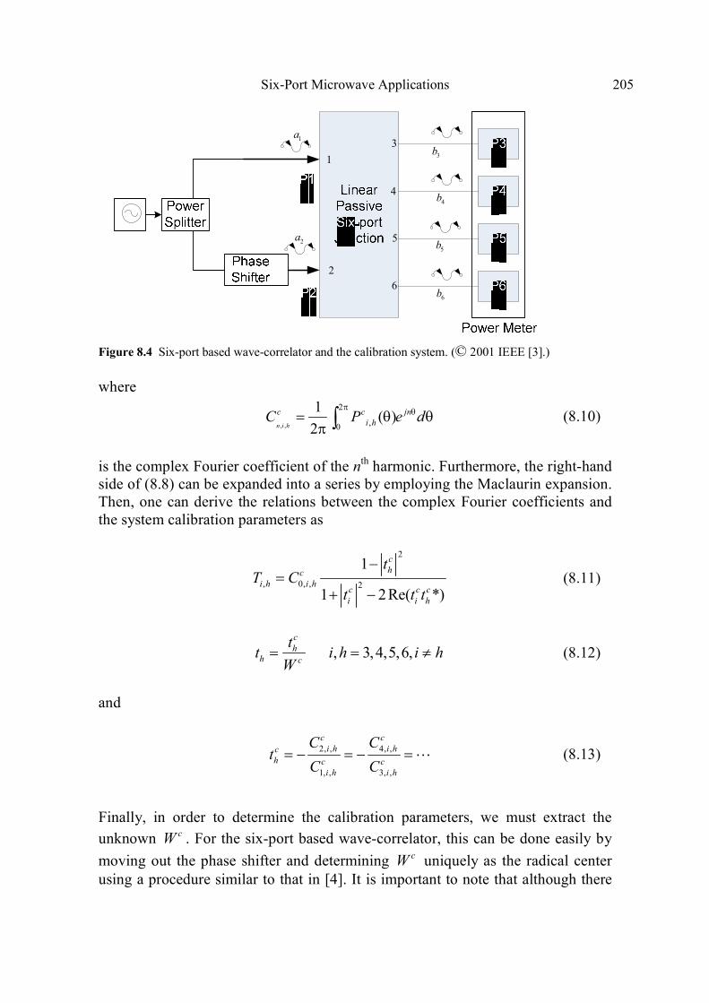
Six-Port Microwave Applications 205
3b
4b
5b
6b
1a
2a
1
2
3
4
5
6
Figure 8.4 Six-port based wave-correlator and the calibration system. (© 2001 IEEE [3].)
where
, ,
2
,0
1( )
2n i h
c c jni hC P e d
π θ= θ θπ ∫
(8.10)
is the complex Fourier coefficient of the nth harmonic. Furthermore, the right-hand
side of (8.8) can be expanded into a series by employing the Maclaurin expansion.
Then, one can derive the relations between the complex Fourier coefficients and
the system calibration parameters as
2
, 0, , 2
1
1 2Re( *)
chc
i h i hc c ci i h
tT C
t t t
−=
+ − (8.11)
, 3, 4,5,6,
ch
h c
tt i h i h
W= = ≠
(8.12)
and
2, , 4, ,
1, , 3, ,
c ci h i hc
h c ci h i h
C Ct
C C= − = − =⋯ (8.13)
Finally, in order to determine the calibration parameters, we must extract the
unknown cW . For the six-port based wave-correlator, this can be done easily by
moving out the phase shifter and determining cW uniquely as the radical center
using a procedure similar to that in [4]. It is important to note that although there

206 The Six-Port Technique with Microwave and Wireless Applications
exist 12 ratios of,i hT , only three ratios are independent of each other.
Consequently, the calibration parameters are three independent real ratios, for
example, 3,4
T , 3,5
T , 3,6
T , and four complex ratios ti , for i = 3, 4, 5, and 6.
2a
1a
Figure 8.5 Six-port circuit components.
After these 11 real calibration parameters are determined during the above
calibration procedure, the six-port based wave-correlator can be operated as a two-
channel receiver and can determine the wave-correlation ratio W using (8.7).
8.2.3 Architecture of a Wave-Correlator
A typical architecture for the six-port wave-correlator is shown in Figure 8.5. The
six-port can be fabricated using four quadrature hybrids. In this wave-correlator
structure, two incident waves are fully utilized for measuring the powers at the
remaining four ports. In the calibration process, the position of the sliding phase
shifter is adjusted. One of the main features of this calibration method is that only
one phase shifter is required, enabling the method to be applied over a broad
frequency band.
8.2.4 Beam Direction Finder Using a Six-Port Wave-Correlator
The six-port wave correlator may be efficiently used in the beam direction finding
applications. The beam direction finder is shown in Figure 8.6. We assume that
two receiving antennas are in the far-field region of the transmitting radiator. In a
far-field case, d>>2D2f/c where d is the distance between transmitting radiator
and receiving antennas, c is the light velocity, and D is the maximum linear
dimension of the receiving antennas. Suppose L is the distance between receiving
antennas, and Φ is the estimated direction angle of the received beam. Assuming
a two-dimensional case with plane wave incidence, the phase of the wave
complex field ratio at two antenna locations separated by a distance L is simply
extracted as [5]

Six-Port Microwave Applications 207
3b
4b
5b
6b
1a
2a
1
2
3
4
5
6
Φ
Figure 8.6 Block diagram for the beam direction finder using a wave-correlator.
2
arg( ) sinW Lπ
= Φλ
(8.14)
where arg( )W is the phase of the wave ratio [3]. Thus, it can be easily deduced
that the beam direction angle Φ is calculated as
1 arg( )sin
2
Wc
fL−
Φ = π
(8.15)
8.2.5 Doppler Estimation Using a Six-Port Wave-Correlator
A system based on the six-port wave-correlator is described in this section to
measure the Doppler frequency of a moving target [3]. As seen, a six-port wave-
correlator determines the vector relation between the two input signals directly by
measuring the power levels. To measure the Doppler frequency of a moving
object and then inferring its velocity, one may use a wave-correlator to evaluate
the relative velocity from the rate of phase variation between the transmitted and
received signals. After the relation between the input and output ports of the six-
port wave-correlator becomes known, the vector relation (amplitude and phase)
between the two input signals is determined by measuring the power levels at the
four output ports. The relation between the input and output ports can be described
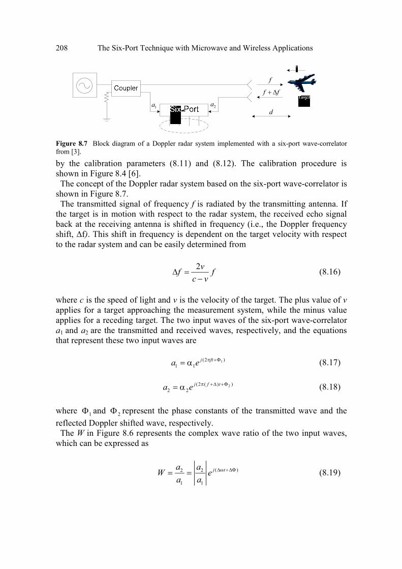
208 The Six-Port Technique with Microwave and Wireless Applications
1a 2a
f f+ ∆
f
d
Figure 8.7 Block diagram of a Doppler radar system implemented with a six-port wave-correlator
from [3].
by the calibration parameters (8.11) and (8.12). The calibration procedure is
shown in Figure 8.4 [6].
The concept of the Doppler radar system based on the six-port wave-correlator is
shown in Figure 8.7.
The transmitted signal of frequency f is radiated by the transmitting antenna. If
the target is in motion with respect to the radar system, the received echo signal
back at the receiving antenna is shifted in frequency (i.e., the Doppler frequency
shift, ∆f). This shift in frequency is dependent on the target velocity with respect
to the radar system and can be easily determined from
2vf f
c v∆ =
− (8.16)
where c is the speed of light and v is the velocity of the target. The plus value of v applies for a target approaching the measurement system, while the minus value
applies for a receding target. The two input waves of the six-port wave-correlator
a1 and a2 are the transmitted and received waves, respectively, and the equations
that represent these two input waves are
1(2 )
1 1
j fta e π +Φ= α
(8.17)
2(2 ( ) )
2 2
j f ta e π +∆ +Φ= α
(8.18)
where 1Φ and
2Φ represent the phase constants of the transmitted wave and the
reflected Doppler shifted wave, respectively.
The W in Figure 8.6 represents the complex wave ratio of the two input waves,
which can be expressed as
( )2 2
1 1
j ta aW e
a a∆ω +∆Φ= =
(8.19)
Six-Port Microwave Applications 209
where 2 f∆ω = π∆ and 2 1∆Φ = Φ − Φ . Obviously, if we denote the phase of the
wave ratio as arg( )W , then
(arg )d W
dt∆ω =
(8.20)
One may extract the velocity from (8.16) and (8.20) as
1 (arg )
4
v d W
c v f dt=
− π
(8.21)
For c>>v, we have
(arg )
4
c d Wv
f dt=
π
(8.22)
From this equation, it is clear that the target’s relative velocity can be determined
by measuring the phase difference between the transmitted and received signals.
8.3 SIX-PORT APPLICATIONS IN DIRECTION FINDERS
In order to obtain the beam direction, the phase difference between the RF input
signals can be measured using the output in-phase and quadrature baseband
signals. It is shown that these signal values will be directly related to the angle of
arrival [7]. A two-dimensional approach to direction of arrival estimation is
presented in this section. Figure 8.8 shows a schematic view of the geometrical
model. The receiving antennas are separated by a distance L. Owing to the angle
of arrival θ, a path difference (∆x) between the two propagation paths will appear.
Consequently, the RF input signals will be phase shifted with respect to each other
by an angle ∆ϕ . As mentioned before, the phase difference between the RF input
signals is directly related to the path difference. The path difference can be
expressed as
x c t∆ = ∆ (8.23a)
or similarly,
2x
∆ϕ∆ = λ
π (8.23b)
Therefore, the angle of arrival θ can be obtained as follows

210 The Six-Port Technique with Microwave and Wireless Applications
sin
2
x
L L
∆ λ ∆ϕθ = =
π (8.24)
x∆
θ
Figure 8.8 Schematic view of the geometrical model.
From (8.23), it can be concluded that the two waves will arrive in phase if the path
difference is zero or an integer number of wavelengths. Furthermore, to avoid any
ambiguity, the distance between the two antennas is chosen to be equal to half the
wavelength at the operating frequency.
Figure 8.9 shows the block diagram of the six-port circuit composed of four 90
degree hybrid couplers [8]. The power reading at each output port (i=1, 2, 3, 4)
can be expressed as
2
5 5 5 6 6 6 . exp( ) . exp( )i i iP S a j S a j= ϕ + ϕ
(8.25)
where 5a and
6a represent the normalized input voltages of the six-port circuit
corresponding to the local oscillator (LO) and RF signals, respectively. In
addition, 5iS and
6iS are the six-port transmission scattering parameters between
the LO, the respective RF input ports, and the four SP output ports. For the same
amplitude of the RF input signals, (a5=a6=a), the output signal powers become
22
6 5exp[ ( )]4
i i iP K a jπ
= + ϕ − ϕ − ζ (8.26)
where Ki is a constant and
exp [ ( 1) ]
4 2i j i
π πζ = + −
(8.27)
represents the solutions of equation 0iP = in the complex plane.

Six-Port Microwave Applications 211
The dc output voltage of an ideal power detector is proportional to the power of
the RF signal magnitude. For the six-port detection circuit presented in Figure 8.9,
the corresponding dc output voltages are proportional to the signal power.
Figure 8.9 Block diagram a typical six-port junction. (© 2004 IEEE [8].)
Supposing that four identical detectors Ki=K are used, the theoretical dc output
voltages are a function of the phase difference between the RF input signals
(6 5∆ϕ = ϕ − ϕ ).
22
sin( ( 1) )2 4
iU K a i∆ϕ π
= − − (8.28)
Each dc output voltage is periodical with 2π and shifted in phase with π/2
multiples compared to other dc output signals [8]. Accordingly, in a six-port
architecture, in-phase (I) and quadrature (Q) signals are obtained as
2
3 1 . cos( )I U U K a= − = ∆ϕ
(8.29a)
2
4 2 . sin( )Q U U K a= − = ∆ϕ
(8.29b)

212 The Six-Port Technique with Microwave and Wireless Applications
ϕ
Figure 8.10 Block diagram of the directional finding circuit.(© 2006 IET [11].)
In these equations, Ui are four six-port detected output voltages, a is the magnitude
of the input normalized wave at one port (a5=a6=a), ∆Φ is the phase difference
between the input normalized waves, and K is a constant that depends on the
power detector characteristics and on the baseband circuit gain.
Using I/Q signals, a baseband vector can be defined in the complex plane by the
following equation
2. .exp( )I jQ K a jΓ = + = ∆Φ
(8.30)
This equation shows that the phase of the Γ vector is equal to the phase difference
between RF input signals ( ∆Φ ). Therefore, this RF phase difference can be
directly measured using both I and Q signals.
By using (8.22) and (8.25), the angle of arrival is presented as
1sin arg( )
∆Φθ = = Γ
π π (8.31)
A block diagram for the beam-direction-finding circuit, according to this
geometrical model, is presented in Figure 8.10 [9]. Two antennas, which feed the
low-noise amplifiers, are connected to the six-port RF inputs. Then the six-port
output signals are detected, amplified, and processed according to (8.25), and
consequently the baseband complex signal (Γ) is obtained. In order to perform
initial direction of arrival estimations, the Γ vector can be directly visualized on an
oscilloscope screen (in XY format). According to (8.31), the position of the point
on the screen is related to the angle of arrival θ. In addition, one can deduce from
(8.30) that if the imaginary part of Γ is equal to zero, the RF input signals are in
phase. Due to an internal phase difference between two transmission paths, an
initial phase adjustment must be performed. After this adjustment, if the antenna
system is rotated in the horizontal plane, the imaginary part of Γ becomes equal to
zero when θ=0o. As a further step, the angle of arrival θ can be calculated using
(8.31).

Six-Port Microwave Applications 213
8.4 SIX-PORT APPLICATIONS IN RADAR
A six-port radar is working based on the concept of wavecorrelation. By
measuring the complex relation of the transmitted and received signals, one may
use this radar to extract the speed and range information of a moving target. The
architecture of a basic six-port radar is shown in Figure 8.11. The signal at port 1
comes from LO and the one at port 2 is unknown. The objective is to obtain a
power reading proportional to the reference signal thus not influenced by the
received signal. This permits correcting the power instability of the signal source
by normalizing the power measurements at the other detectors. Considering
Figure 8.4, detector 3 will be used for this purpose, so3 30 0R q= → = . Then,
(8.4) may be rewritten as
24 4
43 4
3 3
1 L
P KP q
P K= = − Γ
(8.32a)
25 5
53 5
3 3
1 L
P KP q
P K= = − Γ
(8.32b)
26 6
63 6
3 3
1 L
P KP q
P K= = − Γ (8.32c)
These are the equations of three circles centered on qi, whose radius is 3iP .
2 1/a aΓ = is determined by the intersection of the three circles. Constants Ki and
qi are found with a previous calibration.
8.4.1 Six-Port Doppler Sensor
The relations in (8.32) can be used to design a Doppler sensor [10, 11]. Suppose a
signal a1, transmitted by a radar and reflected by a target at a distance d, is
received at the radar after a propagation time T=2d/c, where c is the speed of
light. If the target has a relative speed v to the radar, the propagation time will be
2
d vtT
c
−= (8.33)

214 The Six-Port Technique with Microwave and Wireless Applications
1a 2a
f f+ ∆
f
d
Figure 8.11 Block diagram of a Doppler radar system.
As seen in Section 8.2.5, if the transmit signal can be written as
1 1
j ta a e ω=
(8.34)
where ω is the carrier frequency, then the received signal will be
( ) [( ) ]
2 2 2
j t T j ta a e a eω − ω+∆ω −ϕ= =
(8.35)
where 2 . / ,D v cω = ∆ω = ω and 2 . /d cϕ = ω . The complex relation of the
transmitted and received signals is
2 (2 )2
1 1
. Dj f taae
a aπ −ϕΓ = =
(8.36)
where Γ is a vector that turns at a Doppler frequency, / 2D Df = ω π , and its phase
is proportional to the range. Measuring this rotation, we can determine the
Doppler frequency. Its sign, which indicates whether the target is approaching or
moving away, can be derived by the sense of rotation.
8.4.2 Six-Port Range Sensor
Range information contained in the phase of Γ is somewhat hidden. The
distances measured are much bigger than the wavelengths at the used frequencies,

Six-Port Microwave Applications 215
so the measure will be ambiguous as follows from the expression of (8.35), where
n is unknown
.2 2
dn
c
ωϕ + π =
(8.37)
To avoid this ambiguity, a second signal can be used [10], and the range can be
obtained measuring the phase shift between the Γ coefficients at two frequencies
f1 and f2
1 2
1 2
( ).2
d
c
ω − ωϕ − ϕ = (8.38)
1 2( ) / 2f f− sets the maximum unambiguous range. For example, a range of 100m
requires a frequency shift of 1.5 MHz. This distance measurement procedure
allows determining distance easily, even if the target speed is null. To obtain a
better accuracy in short distances without introducing ambiguity for the long
ranges, three frequencies can be used. When the target becomes closer than a
certain range, the system changes one of the transmitted frequencies so the
frequency difference between them is now larger (e.g., 15 MHz), which gives a
maximum range of 10m.
8.4.3 Radar Structure
Figure 8.12 shows the block diagram of the radar [10]. The microwave oscillator
is frequency modulated by a square signal, which gives the two different
frequencies needed for the range measurement. The modulator and the VCO may
be substituted by noncontrolled oscillators and a fast switch, as only three
different frequencies are needed. A portion of the emitted signal is coupled to the
six-port, which plays the role of a mixer.
Figure 8.12 Block diagram of a six-port radar. (© 2000 IEEE [10].)

216 The Six-Port Technique with Microwave and Wireless Applications
The received signal is injected to the port 2 of the circuit after amplification, and
power detectors are placed at outputs 3–6. The frequency of the four signals that
go into the analog to digital (A/D) converter is the Doppler frequency of the
target. These signals have different phases as they come from different linear
combinations of the signal at port 1 and 2. The signal processing unit finds and
determines the frequency and the range as described before. This unit also
commands the modulation in order to change the frequency shift as the target
becomes closer.
8.4.4 Radar Calibration
It is necessary to find the values of Ki and qi in (8.32) before using the six-port
network. In this section, a straightforward algorithm is proposed [12]. The method
requires a minimum of five loads with a constant absolute value of the reflection
coefficient and unknown but well-distributed phases, followed by three known
loads. As mentioned in previous sections, speed and range are obtained from the
phase of Γ, so its magnitude is not used; hence, it is not necessary to calibrate it.
Even more, they are obtained from phase differences. Doppler frequency,
therefore speed, is derived from the phase difference of two points at the same
frequency, and distance is found with (8.38) from the phase difference of two
points, one at each frequency. Thus, calibration of the absolute phase of is not
required. In this case, the three known loads are now reduced to one, plus two
other loads with unknown magnitude and phase but with a known phase
difference between them.
8.5 ANTENNA MEASUREMENT USING SIX-PORT
8.5.1 Near-Field Antenna Measurement
As seen, the complex signal ratios (including magnitude and phase information)
can be determined using six-port network analyzers. Moreover, they can easily be
designed to operate in a dynamic range of 50 dB. Hence, they are an attractive
choice for near-field measurements [13]. A typical planar near-field antenna
measurement setup system is shown in Figure 8.13. It consists of a scanning frame
housed in an anechoic chamber, a receiver for detection of vector signals, and a
control and process unit. The test antenna radiation pattern can be directly related
to the forward transmission coefficient between the test antenna and a probe
antenna. An ideal six-port receiver would measure the transmission coefficient
directly. Furthermore, since near-field measurement techniques are approximate in
nature [14,15], the six-port network analyzer needs only measure transmission
coefficients with greater accuracy than the errors.
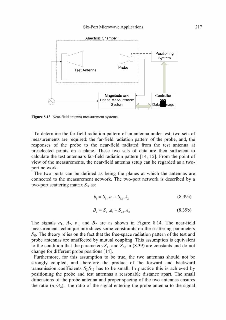
Six-Port Microwave Applications 217
Figure 8.13 Near-field antenna measurement systems.
To determine the far-field radiation pattern of an antenna under test, two sets of
measurements are required: the far-field radiation pattern of the probe, and, the
responses of the probe to the near-field radiated from the test antenna at
preselected points on a plane. These two sets of data are then sufficient to
calculate the test antenna’s far-field radiation pattern [14, 15]. From the point of
view of the measurements, the near-field antenna setup can be regarded as a two-
port network.
The two ports can be defined as being the planes at which the antennas are
connected to the measurement network. The two-port network is described by a
two-port scattering matrix Sik as:
1 11 1 12 2. .b S a S A= + (8.39a)
2 21 1 22 2. .B S a S A= + (8.39b)
The signals a1, A2, b1, and B2 are as shown in Figure 8.14. The near-field
measurement technique introduces some constraints on the scattering parameters
Sik. The theory relies on the fact that the free-space radiation pattern of the test and
probe antennas are unaffected by mutual coupling. This assumption is equivalent
to the condition that the parameters S11 and S22 in (8.39) are constants and do not
change for different probe positions [14].
Furthermore, for this assumption to be true, the two antennas should not be
strongly coupled, and therefore the product of the forward and backward
transmission coefficients S2lS12 has to be small. In practice this is achieved by
positioning the probe and test antennas a reasonable distance apart. The small
dimensions of the probe antenna and proper spacing of the two antennas ensures
the ratio (a1/A2), the ratio of the signal entering the probe antenna to the signal

218 The Six-Port Technique with Microwave and Wireless Applications
entering the test antenna from the receiver, is small. This is assuming that there is
negligible leakage of the signal A2 through the receiver to the probe port and the
probe is not badly mismatched. Finally, under reciprocal conditions (S21 = S12), the
variable S21 is the only scattering parameter changing during near-field
measurements. The principles of designing a receiver to measure this parameter
are described in [13].
8.5.2 Polarization Measurement
A six-port polarimetric measurement system with the use of two dual-polarization
antennas can be realized to measure the polarization states of incoming waves
[16]. A six-port junction used for polarization measurement is shown in Figure
8.15. As can be seen, the two output ports of a dual-polarization receiving antenna
are connected to a six-port network.
Suppose the polarization state of an incoming wave as
V Hb b′′ ′′ ′′= +b v h
(8.40)
where v and h are vertical and horizontal unit vectors.
Figure 8.14 A block of a six-port near-field antenna measurement system. (© 1987 IET [13] .)
The polarization of the incoming wave can be determined by its polarization
ratio as,

Six-Port Microwave Applications 219
/V Hr b b′′ ′′=
(8.41)
The received signals Vb′ and Hb′ from the antenna vertical and horizontal channels
are related to the incoming wave ′′b using
VV VHV V
HV HHH H
R Mb b
R Rb b
′ ′′ = ′ ′′
(8.42)
or
′ ′′=b Rb (8.43)
where R is the transfer matrix of the receiving dual-polarization antenna and
accounts for the imbalance and coupling between its horizontal and vertical
polarization channels. By using six-port theory and according to (8.5), the signals
of the power detectors,
( 3, 4,5,6)ib i = , can be expressed as a linear combination
of two variables Vb′ and Hb′ . Accordingly,
3b and 4b become
3b
4b
5b
6b
1b
2b
1
2
3
4
5
6
3a
4a
5a
6a
Vb′
Hb′
Vb′′
Hb′′
Figure 8.15 Block diagram of a six-port for polarimetric applications. (©1997 IEEE [16] .)
3 11 12
4 21 22
V
H
b M M b
b M M b
′ = ′
(8.44)

220 The Six-Port Technique with Microwave and Wireless Applications
or
′=b Mb (8.45)
where b and ′b are the input and output signals of a six-port network. M is a
matrix dependent on the six-port network configuration and must be determined in
the calibration process.
By using (8.43) in (8.45), b and ′′b are related as
′′=b MRb (8.46)
where ′ =R MR is the receiving transfer matrix. The incoming wave can then be
determined from (8.46) as
′′ ′-1b = R b (8.47)
The calibration procedures to determine the polarization state of an incoming
wave are discussed in [16, 17].
8.6 MATERIAL CHARACTERIZATION USING SIX-PORT
The six-port technique can be used to perform nondestructive permittivity
measurements. The measured permittivity is related to the reflection coefficient by
means of an effective transmission-line model.
This method is suitable for measuring relatively high-loss dielectric liquids.
8.6.1 Measurement System
Figure 8.16 shows a microwave permittivity measurement system. It consists of a
six-port microwave junction and a number of standard microwave laboratory
instruments (power meters, counters, sweepers, and so forth) controlled via a bus
interface. The device under test (DUT) is an open-ended coaxial test probe
immersed in the test liquid kept at a constant temperature [18].
8.6.2 Probe Model Analysis
An open-ended coaxial probe is used in this measurement system. Figure 8.17
shows the equivalent electrical model of the probe immersed into a test medium
with a relative complex permittivity εd. An effective transmission line is used to
model the fringing electric field in the test medium at the extremity of the probe
[19]. Assuming a quasi-TEM propagating mode, the complex admittance at plane
AA' is given by

Six-Port Microwave Applications 221
tan( )
tan( )
E d dL d
d E d
Y jY LY Y
Y jY L
+ β=
+ β
(8.48)
where YL is the admittance at the input of the effective transmission line, Yd is
the characteristic admittance of the effective transmission line, YE is the
terminating admittance at the end of the effective transmission line, βd is
propagation constant in the test medium, and L is the effective transmission line
length.
For physical (radial dimensions of the probe versus wavelength) and practical
(resolution on the measurement of the complex reflection coefficient is
0.5± degree and 0.5± percent in phase and amplitude values, respectively)
considerations, the radiation loss can be neglected [20]. In such a situation, the
terminating impedance is fully reflected impedance (open circuit) and the
admittance YE vanishes. Equation (8.48) becomes
tan( )L d dY jY L= β (8.49)
Figure 8.16 Experimental block diagram of the six-port reflectometer. DC: directional coupler; BP:
bandpass filter; D1, D2, D3, D4: Schottky diode detectors. (© 1989 IEEE [18].)

222 The Six-Port Technique with Microwave and Wireless Applications
A
A’
B
B’
Z
Region 1 Test Medium
dε
dY
L
tYtε
mΓ
Figure 8.17 An open-ended coaxial line homogeneous medium.(©1989 IEEE [18].)
Yd can be expressed as a function of physical parameters of the effective
transmission line as follows:
60 ln( / )
ddY
b a
ε=
(8.50)
where a and b are the inner and the outer diameters of the coaxial probe,
respectively. Furthermore, the admittance YL can be related to the characteristic
admittance of probe Yt and the measured reflection coefficient reported at plane
AA' as follows [18]:
2
2
1
1
t
t
j Dm
L tj Dm
eY Y
e
β
β
− Γ=
+ Γ
(8.51)
where60 ln( / )
ttY
b a
ε= , εt is dielectric constant of dielectric material inside the a
coaxial line (subscript t for Teflon, εt = 2.03-j.004), D is the physical length of the
probe, βt is the propagation constant in coaxial probe, and Γm is the complex
reflection coefficient at plane BB' given by the six-port reflectometer. Substituting
(8.49) in (8.51) and using expression Yd as given by (8.50), one can get

Six-Port Microwave Applications 223
2
2
1cot ( )
2 1
t
t
j Dt m
d j Dm
jc eX g X
fL e
β
β
− ε − Γε =
π + Γ
(8.52)
where 2 dfL
Xc
π ε= , εd is the complex permittivity of the dielectric under test,
D is the physical length of the probe, L is the effective line length, c is the wave
velocity in free space, and f is the measuring frequency. This equation is used to
compute the permittivity from the measured reflection coefficient.
8.6.3 Probe Calibration
In order to evaluate the relative dielectric constant and loss factor of the test
medium, we need to know the probe parameters D and L at each measuring
frequency. The determination of D and L is based on the use of two standard
dielectric mediums [18]. Substituting (8.49) in (8.51), one can obtain
2
2
21
d
t
d
j Lj D m
m j L
ee
e
− ββ
− β
ρ + ΓΓ =
+ ρ
(8.53)
where
t d
t d
ε − ερ =
ε + ε
(8.54)
The two calibration parameters L and D can then be evaluated by using (8.51) and
(8.53) with an iterative computation procedure. This method is also successfully
applied to determine the permittivity of moisture textile [21] and the measurement
of complex dielectric constant of ferroelectrics [22].
8.7 OPTICAL MEASUREMENT USING SIX-PORT
The six-port technique has received some attention from the optical community
after successful application of the six-port technique at microwave frequencies
[23, 24]. The early investigation on using six-port in optics was reported, in which
a six-port optical reflectometer was constructed, using free-space propagation, and
was used to measure optical complex reflection coefficients. The reasons for using
six-port technique in optical applications are probably related to the following
facts. First, the phase measurement of optical devices has been recently required
for many optical measurements. Second, the six-port measurement technique is an
optical domain continuous-wave (CW) interferrometric approach that requires a
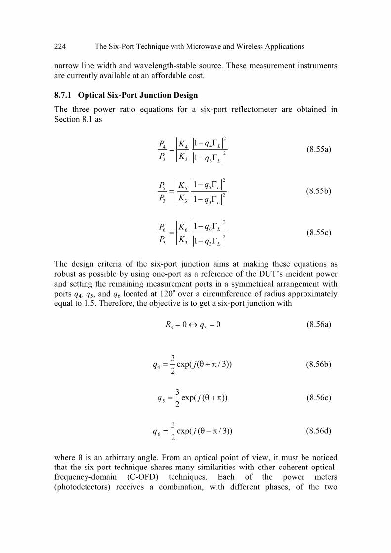
224 The Six-Port Technique with Microwave and Wireless Applications
narrow line width and wavelength-stable source. These measurement instruments
are currently available at an affordable cost.
8.7.1 Optical Six-Port Junction Design
The three power ratio equations for a six-port reflectometer are obtained in
Section 8.1 as
2
44 4
2
3 3 3
1
1
L
L
qP K
P K q
− Γ=
− Γ
(8.55a)
2
55 5
2
3 3 3
1
1
L
L
qP K
P K q
− Γ=
− Γ
(8.55b)
2
66 6
2
3 3 3
1
1
L
L
qP K
P K q
− Γ=
− Γ
(8.55c)
The design criteria of the six-port junction aims at making these equations as
robust as possible by using one-port as a reference of the DUT’s incident power
and setting the remaining measurement ports in a symmetrical arrangement with
ports q4, q5, and q6 located at 120o over a circumference of radius approximately
equal to 1.5. Therefore, the objective is to get a six-port junction with
3 30 0R q= ↔ =
(8.56a)
4
3exp( ( / 3))
2q j= θ + π
(8.56b)
5
3exp( ( ))
2q j= θ + π
(8.56c)
6
3exp( ( / 3))
2q j= θ − π
(8.56d)
where θ is an arbitrary angle. From an optical point of view, it must be noticed
that the six-port technique shares many similarities with other coherent optical-
frequency-domain (C-OFD) techniques. Each of the power meters
(photodetectors) receives a combination, with different phases, of the two

Six-Port Microwave Applications 225
monochromatic waves to be compared (incident and reflected waves at the DUT)
so that each received signal (photocurrent) contains an optical interference term
that is proportional to the cosine of the phase difference; in fact, the six-port
technique could be properly defined, in optical parlance, as being a C-OFD technique with phase diversity [24].
An architecture to implement the optimum six-port junction, as defined by
(8.56), is proposed in [24]. This junction uses multimode interference (MMI)
couplers.
These couplers can be easily constructed in planar lightwave circuit (PLC)
technology. MMI couplers are the basic building blocks of today’s photonic
integrated circuits because of their compactness, low loss, polarization
insensitivity, large bandwidth, high fabrication tolerance, and cascadability, which
allow interconnections to construct more complex structures [25].
The six-port optical architecture is shown in Figure 8.18. It is basically
composed of three MMI: two identical 2×2 couplers (M1 and M2) whose phase
responses are unimportant and one 2×3 120o coupler (M3). The same architecture
contains two interconnecting waveguides: WD is the waveguide (of length LD)
between the reference measurement plane and port 1 of M2, and WC is a
waveguide (of length LC) used to balance the design, as shown next. For the
theoretical analysis presented in this section, the remainder of the connections
between MMIs is considered to be direct (i.e., zero length of interconnecting
waveguides).
The first MMI (M1) acts as a power divider (a nonreflective load has been added
to its port 2) and is used to get a sample of the power incident on the DUT into the
measurement port P3 (so that R3=0). The second MMI (M2) is used as a directional
coupler, i.e., to separate the incident and reflected waves in the DUT that is, at
ports 2 and 3.
As signals have traveled different optical paths, and hence suffered different
phase shifts, a length of waveguide WC is included, as shown in Figure 8.18. To
balance the design, the 2×3 MMI (M3) has been designed so that at any output port
the two input signals are present with equal amplitudes and relative phases of
120o. This is the key component of the six-port junction as it is mainly responsible
for placing the q4, q5, and q6 constants on a circle with a 120o phase difference.

226 The Six-Port Technique with Microwave and Wireless Applications
LΓ
Figure 8.18 An optical six-port architecture. (© 2005 IEEE [24].)
8.7.2 Optical Six-Port Analysis
The S-parameters of the different components of the circuit, shown in Figure 8.18,
are obtained as
21: exp( )D DW S j= ξ
(8.57a)
21: exp( )C CW S j= ξ (8.57b)
31 42
1 2
41 32
exp( )
2, :
exp( ( / 2))
2
jS S
M Mj
S S
ϕ= =
ϕ − π = =
(8.57c)
31 52
3 41 42
51 32
exp( )
3
exp( ( )):
3
exp( ( 2 / 3))
3
jS S
jM S S
jS S
ψ= =
ψ − π
= = ψ − π
= =
(8.57d)

Six-Port Microwave Applications 227
where phase shifts Cξ and Dξ are related to the optical length
( C C effl L n= and D D effl L n= ) of the corresponding waveguides by
,
,
C DC D
l
cξ = ω (8.58)
Both ϕ and ψ take arbitrary values given approximately, near the design
frequency ω0, by the first-order Taylor expansion, as
2 ( )M
o o
l
cϕ = ϕ + ω − ω
(8.59)
3 ( )M
o o
l
cψ = ψ + ω− ω
(8.60)
where 2 2M M effl L n= and
3 3M M effl L n= are the optical lengths of M2 and M3
respectively. For the remaining parameters, the relation ij jiS S= between
scattering parameters linking any two ports is valid by reciprocity theorem, and
we also suppose, for the theoretical analysis, infinite directivity and perfect
matching conditions. Simple analysis of Figure 8.18 yields
1
2 1
31
3 2
21 23 41C
M
W M M
Sb b
S S S′′=
(8.61a)
3 3
4 31 2 32 2
M Mb S a S b′′ ′′= +
(8.61b)
3 3
5 41 2 42 2
M Mb S a S b′′ ′′= +
(8.61c)
and
3 3
6 51 2 52 2
M Mb S a S b′′ ′′= +
(8.61d)
In addition, from Figure 8.18 and taking into account (8.57) we get

228 The Six-Port Technique with Microwave and Wireless Applications
2
2
2
2 21 41 2
2
21 2322 2
12 13
exp( ( 2 ))
2
D
C
D
W M
C DW ML
W M
a S S aja
S Sbb b
S S
′′ =′′ − ξ − ξ − ϕ
⇒ = Γ ′′′′ =
(8.62)
Finally, introducing (8.62) into (8.61) and taking into account (8.57), one finally
obtains the following expressions for the power at the four measurement ports
[24]:
2 2
3 3 22P b b= =
(8.63a)
22 2
4 4 2
12 exp( ( 2 / 3))
6L C DP b b j= = Γ − ξ − ξ − ϕ + π
(8.63b)
22 2
5 5 2
12 exp( ( 2 ))
6L C DP b b j= = Γ − ξ − ξ − ϕ + π
(8.63c)
and
22 2
6 6 2
12 exp( ( 2 / 3))
6L C DP b b j= = Γ − ξ − ξ − ϕ − π
(8.63d)
with
2C Dθ = ξ − ξ − ϕ
(8.63e)
Thus, the proposed topology fulfills the design goals given by (8.56) with the
center point parameters qi located at 120o on a circumference of radius 1.41, and
with an arbitrary angle θ.
References
[1] Engen, G. F., “The Six-Port Reflectometer: An Alternative Network Analyzer,” IEEE Trans. Microw. Theory Tech., Vol. 25, No. 12, pp. 1075–1080, December 1977.
[2] Caron, M., A. Akyel, and F. M. Ghannouchi, “A Versatile Easy to Do Six-Port Based High Power Reflectometer,” Journal of Microwave Power and Electromagnetic Energy, Vol. 30, No.
4, pp. 231–239, 1995.
[3] Yakabe, T., F. Xiao, K. Iwamoto, F. M. Ghannouchi, K. Fujii, and H. Yabe, “Six-Port Based Wave-Correlator with Application to Beam Direction Finding,” IEEE Trans. on Instrumentation and Measurements, Vol. 50, No. 2, pp. 377–380, April 2001.

Six-Port Microwave Applications 229
[4] Yakabe, T., M. Kinoshita, and H. Yabe, “Complete Calibration of a Six-Port Reflectometer with
One Sliding Load and one Short,” IEEE Trans. Microwave Theory Tech., Vol. 42, pp. 2035–2039, November 1994.
[5] Xiao, F., Ghannouchi, F. M., and T. Yakabe, “Application of a Six-Port Wave-Correlator for a
Very Low Velocity Measurement Using the Doppler Effect,” IEEE Trans. on Instrumentation and measurement, Vol. 52, No. 2, April 2003.
[6] Hnyart, B., J. Laurin, R. G. Bosisio. and D. Roscoe, “A Direction-Finding Antenna SystemUsing
an Integrated Six-Port Circuit,” IEEE Trans. on Antennas and Propagation, Vol. 43, No. 12, pp.1508–1512, December 1995.
[7] Tatu, S. O., K. Wu, and T. A. Denidni, “Direction-of-Arrival Estimation Method Based on Six-
Port Technology,” IEE Proc.-Microw. Antennas Propag., Vol. 153, No. 3, June 2006.
[8] Miguelez, C. G., B. Huyart, E. Bergeault, and L. P. Jallet, “A New Automobile Radar Based on
the Six-Port Phase/Frequency Discriminator,” IEEE Trans. Veh. Technol., Vol. 49, No. 4, pp.
1416–1423, July 2000.
[9] Wiedmann, F., “New Structure for a Six-Port Reflectometer in Monolithic Microwave
Integrated-Circuit Technology,” IEEE Trans. Instrum. Meas., Vol. 46, pp. 527–530, April 1997.
[10] Moldovan, E., S. O. Tatu, T. Gaman, K. Wu, and R.G. Bosisio, “A New 94GHz Six-Port Collision Avoidance Radar Sensor,” IEEE Trans. Microw. Theory Tech., Vol. 52, No. 3, pp.
751–759, 2004.
[11] Tatu, S. O., K. Wu, and T. A. Denidni, “Direction-of-Arrival Estimation Method Based on Six-port Technology,” IEE Proc.-Microw. Antennas Propag., Vol. 153, No. 3, pp. 263–269, June
2006.
[12] Zhang, H., L. Li, and K. Wu, “Software-Defined Six-Port Radar Technique for Precision Range Measurements,” IEEE Sensor Journal, Vol. 8, No. 10, pp. 1745–1751, October 2008.
[13] Bialkowski, M. E., and G. S.Woods, “Design and Analysis of a Six-Port Receiver for Use in
Near-Field Antenna Measurements, IEE Proceedings, Vol. 134, Pt. H, No. 6, pp. 515-520, December 1987.
[14] Joy, E. B., W. M. Leach, and D. T. Paris, “Applications of Probe Compensated Near-Field Measurements,” IEEE Trans. on Antennas and Propagation, Vol. 26, No. 3, pp. 379–389, 1978.
[15] Pereira, J. F. R., A. P. Anderson, and J.C, Bennett, “New Procedure for Near-Field
Measurements of Microwave Antennas Without Anechoic Environments,” Proc. IEE, 131, Vol. 6, pp. 351–358, 1984.
[16] Chen T. J., and T. H. Chu, “Calibration and Measurement of a Wideband Six-Port Polarimetric
Measurement System,” IEEE Trans. on Antennas & Propagation, Vol. 45, No. 7, pp.1080–1085, July 1997.
[17] Ghannouchi, F. M., R. G. Bosisio, and R. Hajji, “Polarization Measurements of
Microwave/Millimeter Wave Antennas Using Six Port Techniques,” International Conference on Electromagnetics in Aerospace Applications, Turin, Italy, pp. 283–286, 1989.
[18] Ghannouchi, F. M., and R. G. Bosisio, “Measurement of Microwave Permittivity Using a Six-
Port Reflectometer with an Open-Ended Coaxial Line,” IEEE Trans. Instrum. Meas., Vol. 38, No. 2, pp. 505–508, April 1989.
[19] Cole, R. H., “Evaluation of Dielectric Behavior by Time-Domain Spectroscopy, Part 11:
Complex Permittivity,” J. Phys. Chem., Vol. 79, No. 14, pp. 1469–1474, 1975.
[20] Stuchly, M. A., “Equivalent Circuit of an Open-Ended Coaxial Line in Lossy Dielectric,” IEEE Trans. Instrum. Meas., vol. IM-31, June 1982.

230 The Six-Port Technique with Microwave and Wireless Applications
[21] Pourova, M., R. Zajicek, L. Oppl, and J. Vrba, “Measurement of Dielectric Properties of
Moisture Textile,” 14th Conference on COMITE 2008, pp. 1–4, April 2008.
[22] Ivanov, M., J. Banys, S. Rudys, and R. Grigalaitis, “Measurements of Complex Dielectric
Constant of Ferroelectrics with Six-port Reflectometer in 80-120 GHz Frequency Range,”
Ferroelectrics, Vol. 367, pp. 229–233, No. 1, 2008.
[23] Zhang, Y., G. Colef, Y. Li, and G. Eichmann, “Six Port Optical Reflectometer,” IEEE Trans. Instrum. Meas., Vol. 40, No. 5, pp. 869–871, October 1991.
[24] Fernández, I. M., J. G. Wangüemert-Pérez, A. O. Moñux, R. G. Bosisio, and K. Wu, “Planar Lightwave Circuit Six-Port Technique for Optical Measurements and Characterizations,” IEEE Journal of Lightwave Technology, Vol. 23, No. 6, pp. 2148–2157, June 2005.
[25] Shibata, Y., S. Oku, M. Yamamoto, and M. Naganuma, “Reflection Characteristics and Cascadability of a Multimode Interference 3 dB Coupler,” Proc. Inst. Elect. Eng., Optoelectronics,Vol. 149, pp. 217–221, 2002.

231
About the Authors
Fadhel M. Ghannouchi, a senior Canada research chair in intelligent RF radio
technology, iCORE professor, founder, and director of iRadio Laboratory,
University of Calgary is regarded as one of the foremost authorities in the fields of
RF electronics and radio technology. His current research interests are in their
applications in broadband wireless, satellite, and biomedical sciences.
Other recognitions received by Prof. Ghannouchi include: The Alberta
Professional Engineers Geologists and Geophysicist (APEGGA) Alberta
Ingenuity Fund Research Excellence Award, The Research Excellence Award of
Schulich School of Engineering, University of Calgary, and being elected
distinguished lecturer of the IEEE Microwave Theory and Technique.
For his scientific and technical accomplishments, Dr. Ghannouchi’s peers have
elected him to fellow in The Canadian Academy of Engineering, fellow of The
Engineering Institute of Canada, fellow of The Institution of Engineering and
Technology (IET formally IEE), and fellow of Institute of Electrical and
Electronics Engineers (IEEE).
Prof. Ghannouchi held several invited positions at several academic and research
institutions in Europe, North America, and Japan. He has provided consulting
services to a number of microwave and wireless communications companies
worldwide. His research interests are in the areas of microwave instrumentation
and measurements, nonlinear modeling of microwave devices and
communications systems, design of power and spectrum efficient microwave
amplification systems, design of intelligent RF transceivers for wireless and
satellite communications, and software defined and cognitive radio systems.
Prof. Ghannouchi has published extensively. He has authored two books, was
awarded 7 patents, published more that 400 peer-reviewed articles, given over 50
invited/keynote/plenary conference presentations, trained over 60 master and
Ph.D. graduates, and founded three spin-off companies.
Abbas Mohammadi is currently a professor at the Electrical Engineering
Department of Amirkabir University of Technology and director of
Microwave/Millimeter-Wave and Wireless Communications Research Lab. He
held an invited position at the University of Calgary. His research interests are in
the areas of microwave and wireless communications, six-port techniques,
software defined radio, adaptive transceivers, and MIMO systems. His research
activities led to over 120 publications, 3 U.S. patents, and one Canadian patent.
He is a senior member of the IEEE.


233
Index
ACPR, 120, See adjacent channel
power ratio
Active devices, 7
Active load, 79
Active loop method, 134
Active source-pull measurement,
130
Active source-pull/load-pull, 119
AM/AM characteristics, 145
AM/AM distortion, 120
AM/PM characteristics, 145
AM/PM distortion, 120, 145
ANA. See automatic network
analyzers
Antenna measurement, 17, 199
Array factor, 194
Baseband signal processing, 180
Beam direction finder, 206, 207
Beam direction finding, 206, 212
BER. See Bit error rate
Bilinear mapping., 73
Bilinear transformation, 28
BJT. See Bipolar junction transistor
Boundary limitations, 193
Broadband transceiver, 177
C/IMD3, 120, See carrier to third
order intermodulation products
Calibration, 78, 91
Calibration of TSPNA, 109
Calibration of TSPNA., 107
Calibration parameters, 66, 111
Calibration procedure, 123
Calibration standards, 69, 79
Calibration techniques, 65
Channel interference, 192
Characteristic impedance, 7
CMOS technology, 17
Coaxial reference planes, 136
Coaxial terminals, 96
C-OFD. See coherent optical
frequency domain
C-OFD technique with phase
diversity, 225
Complex reflection coefficient, 86
Conjugate matched, 2
Conversion gain, 141
Coplanar lines, 6
Coupling factor, 9
CW. See continuous wave
DC cancellation, 167
De-embedded reflection coefficient,
74
De-embedded S parameters, 103
De-embedding, 123
De-embedding procedure, 91, 96,
103, 127
De-embedding standards, 128
Delay line, 104
Demodulators, 161
Digital processing, 5
Digital transceivers, 16, 161
Diode Linearization Technique, 84
Direct configuration, 122
Direct conversion, 178, 192
Direct-conversion transceivers, 16
Direction finder, 199
Direction of arrival, 209
Directional coupler, 6, 8
Doppler frequency, 207
Doppler radar system, 208
Doppler sensor, 213
Dual polarization antenna, 219
Dual six-port network analyzer, 145

234 The Six-Port Technique with Microwave and Wireless Applications
DUT, 14, 21, 91, 129, See device
under test
Dynamic range, 65, 81
Embedded reflection coefficient, 31,
104, 121
Embedded reflection coefficient,, 74
Error box, 103, 114
Error box measurement, 78
Error box network, 28, 31
Error box parameters, 121
Error-box procedure, 28
EVM, 178, See error vector
magnitude
Excitation parameters, 98, 109
Fabrication Technologies, 10
Far-field radiation, 217
Field effect transistors (FET), 10
Filters, 6
Five-port receiver, 169
Five-port structure, 168
Forward transmission coefficient, 4,
216
Four standards, 70
Gaussian distribution, 36
Graphical solution, 34
Gunn diode, 10
Harmonic-controlled circuits., 150
Heterodyne, 14, 161
Heterojunction bipolar transistor
(HBT), 11
High electron mobility transistors
(HEMT), 11
High power applications, 18
High power reflectometer, 202
High power six-port junction, 58
Homodyne, 14, 161
IF processing, 5
Image rejection filters, 178
Impulse radio modulator, 183
In band dynamic range, 192
Input reflection coefficient, 4, 135,
148
Intrinsic reflection coefficient,, 81
Ka-band receiver, 189
Linear equations, 96
Linear formalism, 65
Linearization technique, 85
LO power, 192
Load impedance, 135
Load-pull measurements, 119
Load-pulling, 119
Loop coupler, 134
Lossless transmission line, 6
Low noise power amplifier
characterization, 139
Low power consumption, 16
Low-cost transceiver, 17
LRL. See line reflect line
Manual calibration, 81
Matched load, 83
Material characterization, 18, 199,
220
Maximum available power, 2
Measurement applications, 202
Measuring port, 80
Metal-semiconductor field effect
transistors (MESFET), 10
MHMIC. See Monolithic hybrid
microwave integrated circuits
MHMIC Technology, 12
MIC. See Microwave integrated
circuits
Microstrip lines, 6
Microwave applications, 17
Microwave limiters, 145
Microwave network, 3
Microwave network Measurements,
13
Microwave permittivity
measurement system, 220
Microwave transition analyzer
(MTA) techniques, 150
Millimeter-wave, 17
Mixer performance, 141
MMI. See multimode interference

Index 235
MMIC. See Monolithic microwave
integrated circuits
MMIC Technology, 13
Modulation schemes, 182
Modulators, 161
MPSK, 182
MQAM, 182
Multi-band RF stages, 178
Multiharmonic generator, 151
Multiharmonic measurements., 152
Multiport demodulator, 163
Multiport measurements, 21
Multiport modulator, 161
Multiport receiver, 163
Multiport transmitter, 161
Multistandard receiver, 178
Near-field measurement, 17, 216
Network analyzer, 13
Newton-Raphson technique, 71
Noise Figure, 192
Noise measurement, 139
Noise source, 139
Nonlinear formalism, 65
N-port calibration Algorithm, 113
N-port network, 4
NSPNA. See N six port network
analyzer
Numerical algorithm, 71
One-port network, 1
On-wafer load-pull measurements,
136
Optical reflectometer, 223
Optical sampling systems, 150
Optical six-port, 226
Optimal six-port junction, 49
Oscillator Measurements, 143
Output reflection coefficient, 4
Passive circuits, 7
Passive load, 85
Passive load-pull configuration, 131
Passive microwave circuits, 6
Passive source-pull, 129
Passive source-pull/load-pull, 119,
135
Passive tuner, 121
Permittivity measurements, 220
Phase accuracy, 192
Phase distortion, 148, 192
Phase imbalance, 192
Phase noise, 192
Phased array, 195
PIN diode, 10
PLC. See planar light wave circuit
Polarimetric measurement, 218
Polarization measurement, 17
Power amplifier characterization,
141
Power calibration, 33, 86
Power contour, 119
Power detectors, 24, 84
Power division, 7
Power measurements, 15
Power meter, 87
Power readings, 65, 70
Power-added efficiency, 120, 142
Precalibration, 132
Purely reflecting DUT, 104
QAM constellation points, 178
QSOLT, 113
Quadratic equation, 23
Quadrature Hybrid Couplers, 9
Quadrature hybrids, 6
Quasi-optimal six-port junction, 49
Radar, 17, 199
Rat-Race Couplers, 9
Reciprocal, 93
Reciprocity theorem, 227
Reference planes, 99
Reflection coefficients, 69
Reflectometer, 17, 91, 199
Reverse configuration, 122
Reverse transmission coefficient, 4
RF front-end, 182
Ring junction, 53
RMS values, 2
Scattering matrix, 3
Scattering parameters, 1, 4, 5, 14,
15, 21, 31, 53, 91, 92, 95, 96, 98,

236 The Six-Port Technique with Microwave and Wireless Applications
100, 146, 162, 166, 173, 210, 217,
227
Schottky diode, 10
Schottky diode detectors, 79, 84
SDR, 179, See software defined
radio
Self-calibration, 81, 123
Seven standards, 66
Silicon, GaAs, or SiGe fabrication
processes, 13
Six- to four-port reduction
technique, 71, 74
six-port automated network
analyzer., 112
Six-port junction, 33, 39
Six-port measurement techniques,
21
Six-port network analyzer, 14, 91
Six-port radar, 213
Six-port receiver, 113, 216
Six-port receiver (SPR) reference
plane, 114
Six-port reflectometer, 21, 31, 39,
119, 120, 129
Sliding load, 81
Sliding phase shifter, 204
Slot lines, 6
SOLT. See short open load
technique
Source impedance, 135
Source-pull measurement, 129
Source-pulling, 119
SRD. See step recovery diode
SVD. See singular value
decomposition
Switching-mode, 150
Terminated transmission, 7
Thermo-dielectric, 202
Time-domain waveform
measurement, 150, 154
Transmission lines, 6
Transmission parameters, 97
TRL, 113
TSPNA. See three six port network
analyzer
Two-port network, 3, 28, 31, 92,
111, 122, 132, 135, 217
UWB, 182, See ultra wideband
Varactor diode, 10
Variable Test Port Impedance, 143
Vector modulator, 80
Vector network analyzer, 5
VNA. See vector network analyser
Wave comparator, 111
Wave correlation, 204
Wave-correlator, 206
Waveguide six-port junction, 41
Wilkinson Power Divider, 7
Wireless communications, 16
Zero-intermediate frequency (IF),
17