NASA Technical Memorandum 1C0741

T

The Sensitivity of

Synthetic Aperture Radiometersfor Remote Sensing Applications

From Space

D.M. Le Vine

December 1989

(NASA-TM-IO074I) TH_ SENSITIVITY OF

SYNTHETIC APERTURE RAOI_METERS FOR REMOTE

SENSINb APPLICATIONS FROM SPACE {NASA)

59 p CSCL 14B

GS/43

N92-12321

Unclas

0052270

https://ntrs.nasa.gov/search.jsp?R=19920003103 2018-07-10T11:27:14+00:00Z

A _jf

NASA Technical Memorandum 100741

The Sensitivity of

Synthetic Aperture Radiometers

for Remote Sensing Applications

From Space

D. M. Le Vine

Goddard Space Flight Center

Greenbelt, Maryland

National Aeronautics andSpace Administration

Goddard Space Flight CenterGreenbelt, MD

1989

CONTENTS

Page

I. INTRODUCTION ............................................................................... 2

II. THE CORRELATION RECEIVER ................................................................ 4

III. SENSITIVITY OF THE IMAGE .................................................................. II

IV. SELECTED CONFIGURATIONS ................................................................. 16

V. COMPARISON ................................................................................. 22

VI. CONCLUSIONS ............................................................................... 24

ACKNOWLEDGMENT ............................................................................. 25

REFERENCES .................................................................................... 28

APPENDIX A. THE MEAN AND VARIANCE OF THE OUTPUT OF A CORRELATION RECEIVER ....... A-I

APPENDIX B. POWER SPECTRUM OF THE ANTENNA OUTPUT VOLTAGES .......................... B-I

APPENDIX C. THE SAG1TTAL APPROXIMATION .................................................... C-I

APPENDIX D. COORDINATE TRANSFORMATIONS .................................................. D I

APPENDIX E. RELATIONSHIP BETWEEN BRIGHTNESS AND EI.ECTR1C FIELD INTENSITY . ........... E-I

APPENDIX F. THE SYNTHESIZED BEAM .......................................................... F-I

iii PRECEDING PAGE BLANK NOT FILMED

THE SENSITIVITY OF SYNTHETIC APERTURE RADIOMETERS FOR

REMOTE SENSING APPLICATION FROM SPACE

by

David M. Le Vine

PREFACE

Aperture synthesis offers a means of realizing the full potential of microwave remote sensing from space by helping

to overcome the limitations set by antenna size. The result is a potentially lighter, more adaptable structure for applications

in space. However, because the physical collecting area is reduced, the signal-to-noise ratio is reduced and may adversely

affect the radiometric sensitivity.

Sensitivity is an especially critical issue for measurements to be made from low earth orbit because the motion of

the platform (about 7 km/s) limits the integration time available for forming an image.

The purpose of this paper is to develop expressions for the sensitivity of remote sensing systems which use aperture

synthesis. The objective is to develop basic equations general enough to be used to obtain the sensitivity of the several

variations of aperture synthesis which have been proposed for sensors in space. The conventional microwave imager (a

scanning total power radiometer) is treated as a special case and the paper concludes with a comparison of three synthetic

aperture configurations with the conventional imager.

I. INTRODUCTION

Microwave remote sensing from space offers the potential for measuring many of the parameters important for

understanding the environment of the earth on a global scale (Butler et al., 1988; Murphy et al., 1987), Among the

parameters which can be measured are sea surface temperature (Wilheit and Chang, 1980), ocean salinity (Thomann,

1976), soil moisture (Wang et al., 1983), and sea ice concentration (Swift et al., 1985). Microwave remote sensing has the

advantage that it can be done in the presence of cloud cover, permitting measurement of these parameters in regions inac-

cessible to visible and infrared sensors. Furthermore, because of the strong sensitivity of microwave radiation to the

presence of water and the ability of microwave radiation to penetrate beneath the surface, unique information is available

at microwave frequencies of compliment remote sensing at visible and infrared frequencies.

However, realizing the full potential of passive microwave remote sensing from space requires putting relatively

large antennas in space. The apertures required for microwave sensors are large compared to those required of visible and

infrared sensors because of the much longer wavelength in the microwave portion of the spectrum. For example, antenna

size is the factor limiting the implementation of an L-band radiometer in space to measure soil moisture, and antenna size

is an important factor limiting development of a microwave sensor to fill the gaps created by clouds in present-day visible

and infrared soundings of the atmosphere.

A possible means of overcoming this size limitation is to use aperture synthesis (e.g., Le Vine and Good, 1983;

Thompson, Moran and Swenson, 1986). This is a technique in which correlation receivers are used to coherently measure

the product of the signal from pairs of antennas with many different antenna spacings. For distant sources, it can be

shown that this correlation function is proportional to the Fourier transform of the intensity of the source at a frequency

which depends on the spacing between the antennas. By making measurements at many different spacings one determines

the Fourier spectrum of the source; then a map of the source can be obtained after all measurements are complete by in-

verting the transform. The resolution obtained in this manner is determined by how well the correlation function has been

measured, not by the size of the antennas used. In principle, one can obtain very high-resolution maps of the source by

measuring at many different baselines using relatively small antennas.

This technique has been successfully employed in radio astronomy to obtain very high-resolution maps of radio

sources in what is called "earth rotation synthesis" (Swenson and Mathur, 1968; Brouw, I975; Hewish, 1965; Thompson,

Moran and Swenson, 1986). The Very Large Array in Socorro, New Mexico is an example (Napier et al., 1983). Several

versions of this technique have also been proposed for remote sensing from space. These include a proposal (Schanda,

1976,1979)inwhichthebaselineischangedbymakingmeasurementsatdifferentfrequencies,aconcept(Mel'nik,1972)

involvinga movingsystemwithasinglefixedbaselineinwhichmeasurementsmustbemadeatseveraldifferenttimede-

lays,andamodificationwhichemploysascanninglineararraywhichisrotated(C.Wiley,privatecommunications).

MorerecentvariationsincludeaconfigurationresemblingaMillscrossinwhichmultiplebeamsareformedwithantenna

elementsalongeacharmof thecross(Milman,1988);avariationresemblingMel'nik'sconfiguration(Mel'nik,1972)us-

ingcontiguousparallelbeamsandmatchedfiltering(HughesAircraftCo.,privatecommunications)andfinally,ahybrid

realandsyntheticaperturesystemwhichusesrealantennasto obtainspatialresolutioninonedimensionandaperturesyn-

thesisto obtainresolutionin theotherdimension(LeVineetal., 1989;Swiftetal., 1986).

Amongthemostimportantissueswhichmustberesolvedto determinetheviabilityof aperturesynthesisfor remote

sensingfromspaceis thesensitivity(AT)whichcanbeachievedwithaparticularconfiguration.Sensitivityisanespecial-

ly criticalissuefor measurementsfromlowearthorbitbecausethemotionof theplatform(about7 km/'s)limitsthein-

tegrationtimeavailableforimaginga particularscene.Theproblemisespeciallyperniciousbecausethehigherthe spatial

resolution required the less time is spent by the spacecraft over the scene. Other factors being constant, sensitivity de-

pends on the actual (i.e. physical) collecting area of the antenna system employed. But the goal of aperture synthesis is to

reduce the physical collecting area needed for a given spatial resolution. The sensitivity lost in this trade can, in many

applications, be reclaimed by increasing the integration time-bandwidth product. However, this is not always possible for

sensors in space because platform motion restricts the integration time, and requirements on the field-of-view and the

problem of RFI restrict the bandwidth (Thompson and D'Addario, 1982). This trade-off between physical aperture and

sensitivity was the motivation behind the hybrid real-and-synthetic aperture system mentioned above which was conceived

as a means for achieving the sensitivity needed for soil moisture measurements from space (Le Vine et al., 1989; Ruf et

al., 1988).

The purpose of this paper is to develop expressions for the sensitivity of remote sensing systems which use aperture

synthesis. The objective is to develop basic equations general enough to be used to obtain the sensitivities of the several

variations which have been proposed for sensors in space. The analysis is done in two parts: the first is a derivation of

the sensitivity of the detector used to measure the signal from an individual pair of antennas (a coherent correlation

receiver) and the second is the derivation of the sensitivity of the pixels in the final image. This is illustrated in Figure 1.

On the left are shown two antennas viewing the scene. In aperture synthesis the antenna output voltages, V i, are multi-

plied together and averaged. The middle panel of Figure 1 shows the schematic of a detector which makes this measure-

ment.Theoutputof this detector, Yij, is a point in the Fourier transform space of the scene; and the scene itself is

obtained by doing an inverse Fourier transform on the set of measurements {Yij}" This is done by the processor (far right)

in Figure 1. Many variations on this basic theme are possible. The variations may differ only in how the baselines are dis-

tributed in space or may involve subtle variations in how the signal processing is implemented. However, in each of the

variations mentioned above, the correlator is a common element and the variations may all be cast in the form of Figure 1

with different processors. Hence, this paper will begin (Section II) with a discussion of the correlation receiver, deriving

first the signal-to-noise ratio (SNR) and then the temperature sensitivity (AT) of the output. Then (Section liD, an expres-

sion will be derived for the sensitivity in the final image, assuming that the processor is a discrete Fourier transform on

the set of correlator outputs. It will be shown that in the most general case, the sensitivity may not be the same at each

pixel in the image. Finally (Section IV), these results will be used to compare several of the variations of aperture synthe-

sis mentioned above as potential candidates for remote sensing from space. The sensitivities of these configurations will

also be compared with that obtained using a scanning, total power radiometer. The later result is obtained as a special

case of the analysis done above.

II. THE CORRELATION RECEIVER

In aperture synthesis the coherent product (amplitude and phase) of the output voltages from a pair of antennas is

measured for many pairs at different antenna spacings, and then an image is formed by processing this set. Ultimately,

one is interested in the signal-to-noise ratio and sensitivity of the image, but as pointed out above, it is convenient to do

the calculations in two steps, beginning with the receiver and then doing the calculations for the image. In this section,

expressions are derived for the signal-to-noise ratio and the sensitivity of the correlation receiver.

A. Signal-to-Noise Ratio (SNR)

A schematic of the ideal correlation receiver is given as part of Figure 1 (middle). The receiver forms the coherent

product of X i and Xj which represents the voltages at the output terminals of the k-th pair of antennas. As part of the sig-

nal processing, these voltages would normally be amplified, filtered and mixed down to a convenient IF for further

processing. The transfer functions, H i and Hj represent the cumulative effect of this processing. N i and Nj represent the

equivalent noise in the circuit referred to the input and HLp is a low pass filter which represents the averaging (integra-

tion) which is done after the muitipiic_!i6n.

The input X i will be written in the form X i = Xi ° + xi where Xi" is the antenna output from a (perhaps hypotheti-

cal)constantbackgroundagainstwhichchangesaremeasured.Thevoltagexi is thechangerelativetothisbackground

whichit isdesiredto detect.Thesignalri attheinputtothereceiver(Figure1)isthesumoftheantennaoutputandthe

systemnoise:ri = Xi° + Ni + xi.

Definethesignal-to-noiseratiotobe(e.g.,Tiuri, 1964)themeanchangeinoutputduetothepresenceof thesignal

dividedbythestandarddeviationof theoutputwhenthesignaliszero(i.e.,dividedbytheRMSnoise).Usingthisdefi-

nition,theSNRfor the receiver output, yij(r), is:

< y_j(X° + N + x) > - < y_j(X° + N) >(1)SNR - I

x/< y2j(XO + N) > - < y_j(X° + N) >2

Expressions for the moments of y_j needed to evaluate Equation 1 can be obtained from Figure I using standard

procedures (e.g., Appendix A). Since the signals ri(t ) are the result of thermal noise, it is reasonable to assume that they

are very broadband compared to the (bandpass) filters Hi(v). In addition, assuming that HLp(v) is very narrow band com-

pared to the Hi(v), it can be shown (Appendix A) that:

oo

< YiJ(r) > = Sij(v) HLp(0)- I Hi(v) Hj*(v) dv

--oo

Var[y,j(r)l = < yij2(r) > _ < yij(r ) >2

oo ot_

= [Sq2(vo) + Sii(vo) Sjj(vo) ] I Hi2(v) Hj2(v) dv I HLp2(v) dv

-oo -oo

(2a)

(2b)

where Sij(v) is the Fourier transform of the correlation function, Rij('r) = < ri(t) rj*(t + 'r) >, and % is the center fre-

quency of the bandpass filters. The preceding expressions ignore "fringe washing," a problem which becomes important

as the passband of Hi(v ) becomes large (Thompson and D'Addario, 1982). In employing Equations 2 it is convenient to

make the following definitions:

Hi(v) Hj*(v) dv

--IX,B =

I [ Hi(v ) Hj(v) 12 dv

H2Lp(O)7=

oa

f H2Lp(V dv

(3a)

(3b)

where B is called the "noise bandwidth" of the receiver (Tiuri, 1964; Thompson et al., 1986) and r is the equivalent in-

tegration time of the low pass filter (Kraus, 1966; Tiuri, 1964). =

Now, substituting Equations 2 into Equation I and using the definitions in Equations 3, one obtains the following

expression for the signal-to-noise ratio of the receiver:: = =

S N R = Sij(V) '_ (4)

4s_j2(Vo)+ S.(v o) S_(vo)

In order to proceed further, the spectral densities, Sij(v), are needed. These are needed in two cases: a) when the in-

put is the ambient background plus system noise (r i = Xi" + NiL and b) when the input is the ambient background plus

system noise plus the signal to be measured (r i = Xi ° + N i + xi). It will be assumed that the noise N i in the two chan-

nels of the radiometer are independent, and are independent of the ambient noise, Xi °. Then, in the first case (r i = Xi ° +

NiL one obtains the following correlation functions:

Rijlr_) = < [ Xi° + Nil [ Xj" + Nil > (5a)

< Xi° >Xj °

Rii(r) = < IX", + Ni]2 > (5b)

= < Xi ° Xi° > + < Ni 2 >

where < x i xj > has been used as a shorthand notation for the correlation function < xi(t)xj*(t + r)> and the complex

conjugate (*) has been dropped because the signals are real. If the noise and ambient signal in the two channels are the

same, the results simplify and one may write:

6

Rii(r')= Rjj(r) = < Xo2> + < No2> (6a)

= No.In thesecondcase(ri = Xi° + N i + xi), only the cross terms (i _: j) arewhere Xi° = Xj° = X o and N i = Nj

needed in Equation 4. One obtains:

Rij(r ) = < [Xi° + N i + xil[Xj ° + Nj + xj] > (6b)

= < Xi ° Xj ° > + < x i xj >

where it has been assumed that < xi Xj ° > = 0.

Now, the spectral densities Sij(v) needed in Equation 4 are obtained by Fourier transforming the Rij(r) in Equations

6a and 6b. Denoting this Fourier transform by double brackets, < < > >, Equation 4 becomes:

< < xixj> >S N R = _ (7)

"Vt< < XiOXjO> > + [ < < Xo2 > > + < < No2 > > ]2

The Fourier transforms needed in Equation 7 can be derived following straightforward procedures (e.g., Appendix

B; also see Fomalont and Wright, 1974). It turns out that the transforms are proportional to the spatial Fourier transform

of the scene evaluated at a frequency n = voL/c where L is the distance between antennas. Since Xi ° is the output due to

the ambient background, which by assumption is constant and the same for each antenna, the spectrum, < < Xi°Xj ° > >

is zero except possibly at )7 = 0. Thus, when r/ , 0, the SNR is:

< < XiX j > >SNR = X/_B r (8)

<< Xo2 >> + << No 2 >>

When T/ = 0 the correlation radiometer (Figure I) is degenerate and it becomes a total power radiometer. In this case, the

analysis follows as above except that r i = rj and Hi(v) = Hj(v). In this case, one obtains:

<< Xi2 >>

S N R = _ (9)

<< Xo2 >> + << No 2 >>

which differs from Equation 8 only by a factor of 2 (Tiuri, 1964; Kraus, 1966).

B. Sensitivity

The sensitivity of the correlation receiver is obtained by setting the left-hand side of Equation 8 to unity (i.e., SNR

= 1) and solving for the fluctuation < < xixj > > required to produce this SNR. However, before doing this it is

7

convenienttochangethenotationin theprecedingexpressionstothatcommonlyusedin radioastronomyandremote

sensingapplications.

Toproceed,noticethattheFouriertransform,< < xixj > >, canbewrittenin thefollowingform(AppendixB;

alsoseeSwensonandMathur,1968):

+!

I P.(q) B,(q) exp(-j27r].q) dq< < XiXj> > = (Z°Ae/2) "_/1 - q2 _ %.9 w B

-I

(10)

where 71= L (Vo/C) and L is the vector distance (i.e. "baseline") between the antennas, Z o = _ is the impedance of

free space and A e is the effective receiving area of the antenna. (In the general case < < xi xj > > is a complex num-

ber; however, its complex conjugate is obtained trivially by interchanging antennas. Hence, one can always form a real

signal to use in calculating the signal-to-noise ratio by averaging these two values: Re < < XiXj > > = [ < < XiXj > > 4-

< <XjXi> >]/2. This value will be used in Equation 8 to obtain the SNR. Additional discussion and an example of this

point is given in Section 11111.4.)

Before substituting into Equation 8, it is convenient to put Equation 10 into a more symmetric form by defining a

normalized brightness temperature B,(q) as follows:

B(q_)

B.(q_) - [h-/,.kTa] B(q..)

B,(q.)

(11)

where Bo(q) is the brightness of a constant thermal source of temperature T B (i.e., assuming that the Rayleigh-Jeans law

applies to this source). With this definition, Equation 10 becomes:

< < xixj> > = Z"[kTB/X2IA_ l

and defining 0(_) to be the following integral:m

P.(q_) B.(q. )

, exp(-j27r_oq) dq41 - q2 _ q_ - - -

(12)

0(TI) = Re

+I

S-I

P.(q) B.(q)

41 - qx" - qy2exp(-j2r-_'q-)'d_(13a)

oneobtains:

Re< < XiXj ) > ----- Z o [kTB/k2] A e O(rt)

Notice that when Bn(q) = 1 and 7/ = 0 (i.e., the special case of a total power radiometer), then 0(.7/.)reduces to the

"solid angle" of the antenna used in the measurement (Kraus, 1966):

(13b)

fie = I P.(O, _) sin(O) dO dq_(14a)

+1

I Pn(q) qy2dqw "D

x/1 - qx2 -

-I

(14b)

= )`2 / Ae (14c)

The transformation between the spherical coordinates (0, 6) and the direction cosines (qx, %) is straightforward ( Appen-

dix D or Swenson and Mathur, 1968) and a derivation of Equation 14c can be found in Kraus (1966).

It is possible to obtain an explicit expression for < < Xo 2 > >, due to the ambient background, in terms of the no-

tation introduced above. In particular, since < < Xo 2 > > is measured at _7.= 0 and due to a constant (B n = 1), one has

< < Xo2> > = Zo[k Tx / ),2] Ae = Zo k T x. Finally, assuming that the internal system noise is due to an equivalent

source, but with temperature T N, one can write: < < No2 > > = Z,, k T N. Now using these expressions and Equations

13 and 14c in Equation 8, the SNR can be written:

T a 0(r/)S NR - _ x/_B r (15)

Tx + TN fie

Finally, the sensitivity of the correlation radiometer can be obtained by solving for the T B which yields a SNR = I.

Calling this value AT, one obtains:

Tsys fleAT=-

B r 0(2/)

(16)

where Tsy s = T x + T N is the total "system" noise. Notice that the sensitivity, AT, depends on the antennas used in this

measurement (i.e., on their solid angle, fie), on the baseline between antennas ( _. ), and also on the structure of the

source through 0( 9 .

C. Special Cases

Equation 16 is a general expression and it will be used below to analyze several potential sensor systems which use

aperture synthesis. However, before doing so several special cases will be considered to show that Equation 16 includes

the standard results.

1. Point Source

First, consider the case when the scene is a point source. In this case, assuming that the point source is well within

the main beam of the antenna so that Pn(q)/ _/1 -- qx2 -- qy2 _= l, one obtains 00!) =cos(2 7r r/oqo ) where qo is a unit

vector pointing toward the source. Using this result, the sensitivity is:

Tsys fieAT = point source (I 7)

B r coS(So)

whereSo = 2 r r/._qo. Notice that the singularity at coS(So) = 0 is only apparent because cos(So)= 1 near the main beam

of the antenna, where it has been assumed that the point source is located. Equation 17 is identical to that derived by

other methods (e.g., Tiuri, 1964; Kraus, 1966; chapter 7) except for the effect of the receiving antenna, fie, which

appears explicitly here. This factor doesn't appear (it is unity) if it is assumed that T,y._ = Tx + TN is the noise tempera-

ture of an equivalent point source (see below) as is done in the references cited above (e.g., Kraus, 1966).

2. Total Power Radiometer

As a second check, consider the case of a total power radiometer. The derivation follows as above but begins with

Equation 9 for the SNR and uses __ = 0 (zero baseline) in Equations 10, 12, 13 and 15. The result is:

Tsys f_c&T = Total Power (18a)

B,/'B,/'B,/'B,/'B,/_70(0)

In the special case of a uniform source which fills the beam of the antenna (B = 1), one has 0(0) = tic and the expres-

sion for the sensitivity becomes:

TsysAT-- Distributed Source (18b)

which is the classic result (Kraus, 1966; Ulaby et al., 1981). In this case the sensitivity is independent of the antenna

lO

aperture.However,noticethatin thecaseofa pointsource(locatedverynearthemainbeamof theantenna)onehas

0(0) = 1 and the sensitivity is:

TsysAT = _ fie Point Source

a4-ff-7

which depends on the antenna aperture. Clearly, the larger the antenna aperture (fie

measurement will be to a point source.

(18c)

= X2 / Ae) the more sensitive the

3. Noise Temperature Using Equivalent Point Source

Finally, note that in each of the examples above, the equation for AT depends on the definition of Ta and T N . In

particular, these could have been chosen to be the temperature of an equivalent point source rather than a distributed

source (as was done above). Assuming they are due to a point source near the main beam of the antenna (i.e., at _% =

0), then << Xo2 >> = ZokT x /f/eand << No2 >> = ZokT N / fie. The derivation of AT in this case follows as

above, and the results can be obtained from Equations 15 through 18 by multiplying each equation by 1/fi e. For example,

Equation 17 becomes AT = [Tsys/X/'_]/cos(q_ o) and Equation 18b becomes AT = [T_yJX/'_/_ e but now Equation 18c

is AT = Tsys/B_'_.

IH. SENSITIVITY OF THE IMAGE

Equation 16 is the sensitivity of the output of a coherent correlation receiver (Figure i) with an arbitrary, but fixed

baseline _/. In aperture synthesis, measurements are made at many baselines and then an image of the scene is constructed

by taking a Fourier transform of these measurements (a discrete Fourier transform on the discrete set of measurements).

In this section, an expression will be derived for the sensitivity in the final image when the processor in Figure i is a dis-

crete Fourier transform (DFT). This provides a basic formula from which several variations of aperture synthesis can be

discussed (Section IV to follow).

For simplicity, assume that the measurements (receiver outputs, y,j) are made at antenna baselines which can be

mapped onto the coordinates of a Cartesian grid with uniform spacing, d_ and dy along each axis, respectively. That is,

assume that the measurements can be mapped onto the points ( m d_, n dy ) where m = 0, 1, 2 .... M - 1 and n = 0,

I, 2 .... N - 1. Also, let Iron be the intensity in the mn-th pixel of the image. Then, with the processor being considered

here, Iron is the two-dimensional discrete Fourier transform of the receiver outputs: Imn = DFT [Ymn]"The objective of

11

thissectionis to deriveanexpressionfor thesensitivityof the Im. tO changes in the scene.

A. Signal-to-Noise Ratio (SNR)

The initial step is to calculate the SNR and then the sensitivity is obtained by setting the SNR to unity. Adopting the

same definition of signal-to-noise ratio for the image as was used for the receiver, one has:

< Imn(X ° + N + x) > - < Imn(X ° + N) >S N R -- (19)

if< I2mn(X ° + N) > - < Iron(X° + N) 2 >

In this notation, Imn(X ° + N) = DFT [Ymn(X° + N)] is the intensity of the mn-th pixel in the image when the input is

the ambient background (X °) plus system noise ( N ). < Im.(X° + N) > is a constant (d.c.) background noise in the im-

age due to system noise and the ambient scene. The "'signal" is the change in the scene relative to this ambient back-

ground and is due to x.

Since the DFT is linear, the numerator in Equation 19 can be found immediately from Equations 2a, 5a and 6b.

< lmn(X ° + N + x) > - < I,,,n(X" + N) > = DFT{<<Xn, X.>> } HLp(0 )

One obtains:

i Hm(V) Hn*(v) dv

oo

(20)

in order to evaluate the denominator more information is needed about the output noise, y.m(X" + N). It is straightfor-

ward to show that <y.,.(X" + N)> = 0 for all non-zero baselines (e.g., Equations 2a, 5a, and the discussion following

Equation 7). In addition, it will be assumed that the y,,m(X" + N) are all independent and identically distributed. Then

substituting into the definition of the discrete Fourier transform and using Equation 2b, one obtains:

< 12m.(X ° + N) > - < I,,,.(X" + N)-" > (i/MN) I 2 .... "= <y,..(X + N)> - <y,..(X + N)>- I (21 a)

"_ V= (i/MN) [ S-,.n(.) - Snn(vo) Smm(vo) 1

oo oo

I SH,.(v) Hn*(v) dv H-kp(v )

--oo _o

dv (2 l b)

where M and N are the number of elements in each dimension of the discrete transform. Notice that the subscript "'mn"

has been kept in the equation above, although by assumption the result is independent of m and n (except possibly at m

12

= 0 and n = 0 where the receiver is degenerate and becomes a total power receiver). Now, using Equations 5a and 5b

and 6a in Equation 21b and using the definitions given in Equations 3, one obtains:

DFT { < < Xm Xn > > }

S N R = 42 M N B r (22)

<< )(o2 >> + << N 2 >>

Before calculating the sensitivity, it is convenient to rewrite Equation 22 in more conventional notation as was done

above (Section liB). Following the same procedure (i.e., defining a normalized brightness Bn(q) as in Equation 11 and

then using Equation 12), one obtains:

DFT{ < <XmX,> > } = Z_,[k TBI [Ae/X2]

+!

S P,(q_) B,,(q...)V 1 _ q2 _ %2

I

G(qm n -- q) dq

= Zo[k T B] [Ae/_.2]O(m,n)

where the following definitions have been made:

G(qm n - q..) = OFT {w exp(-j21r r/A.q_)}

(23)

(24a)

+1

f P.(q_) B.(q)O(m,n) -- G(qm n - q) dq (24b)x/l - q2 _ %2 - - -

-!

The factor, w, introduced in Equation 24a is an arbitrary "weight" which has been included in the DFT for complete-

ness. It can be assigned arbitrarily to shape G(q) or can be used to account for redundant measurements. The vector .,qm.,

identifies each pixel in the image. Its components qm,, = (qm, qn) in the special case of uniformly spaced baselines are qm

= m _, / d_ M and q, = n _, / dy N. (See Appendix F).

Now, assuming that << Xo2 >> = Z okT x and << N 2 >> = ZokT N ,asdonein Section liB, and using

Equation 23b, one obtains the following result for the signal-to-noise ratio:

TB O(m,n)

S N R - _ x/2 M N B r (25)

Tx + TN f_e

where 12e is the "solid angle" of the antennas used in the measurements as defined in Equations 14. The sensitivity of the

image is obtained by setting the SNR = I and solving for the signal T B required to achieve SNR = 1. Calling this signal

13

AT, one obtains:

ATTsys 1 fie

_ O (m,n).(26)

Notice that since O (m,n) depends on m and n, the SNR and sensitivity, AT, may be different for each pixel. However,

while this is true in general, it is not a problem for the special cases most commonly encountered in practice. Examples

will be given in the special cases to be discussed below.

B. Special Cases

In the case of uniformly spaced measurements, G(q) has the form of the array factor encountered in the analysis of

uniform, linear antenna arrays (Appendix F; also, see Jordan and Balmain, 1968). In applications such as remote sensing

from space, the number of individual antennas in the synthesis array is likely to be large (e.g., Le Vine et al., 1989), in

which case G(qm n - q) will be a rapidly varying function in comparison to Pn(q) with its support near q_mn"Hence, near

the center of the image where ] qmn I < < 1 one obtains:m

O(m,n) =

+!

SI

B,,(q.._)G(qm, n - q) dq (27)

This is just the expression for the power received by an antenna with the power pattern, G(q), when viewing the sourcew

B_(q) (e.g., Kraus, 1966; Collin and Zucker, 1969). Hence, close to the center of the image, O(m,n) Will depend on

(m,n) only to the extent that the scene, B,(q), changes from pixel to pixel.

Before proceeding, it is convenient to define a solid angle, fly. and an equivalent area, Asyn, for the "synthesized

beam." In light of the discussion above (Equations 24 and 27) and in analogy with Equations 14, the following definitions

are made:

I p.(q)fl_Yn = V'I _ qx2 _ qy2

I

G(q) dq (28a)

= _2 / A yn (28b)

14

Withthesedefinitions,Equation26canbewritteninaparticularlyappealingforminafewimportant,specialcasesas

discussedbelow.

1) Distributed Source

First, consider the case of a distributed source which is constant over the dimension of one pixel. Then O (m,n) -=

fZsy n = h 2 / Asy n and Equation 26 becomes:

Tsy s ,1 Asy n

AT - (29a)M,/W'gAe

This is the form commonly found in radio astronomy applications (Napier et al., 1983; Thompson et al., 1986).

2) Point Source

Next, consider the case of a point source located in the main beam at qm.,"

and Equation 26 becomes:

In this case, one has O (m,n) _ i

Tsy s 1

AT = _ _ _2 (29b)

3) Zero Redundancy

Additional insight can be obtained by examining the factor, MN, in Equations 29. Consider n antennas and suppose

that measurements are made at all possible antenna pairs. There are n(n - 1)/2 different pairs. If no pairs have the same

baseline (and the baselines are uniformly spaced), then this arrangement is referred to as a "zero redundancy" array. In

practice, more than n antennas would be required to achieve the n(n - I)/2 baselines because zero redundancy arrays

have been found in only a few cases (e.g., Moffet, 1968). However, it is convenient to assume a zero redundancy array in

order to obtain an expression for AT which explicitly shows its dependence on the number of individual antennas in the

synthesis array. Hence, let MN = n(n - I)/2 and, since n is likely to be large for any practical application in remote

sensing from space, one may further simplify by writing MN --__n2/2. Thus, in the case of a zero redundancy array of n

antennas, Equations 29 can be written:

Tsys Asyndistributed source

B,,rff7n Ac

AT =

Tsys fiepoint source

B4-ff-;n

(30a)

(30b)

15

Equation30ais theexpression commonly quoted in the literature on applications to radio astronomy (e.g., Napier et al.,

1983). Clearly, in either case (point source or distributed source), reducing the product, n A e , worsens the sensitivity.

Hence, in applications to remote sensing from space there is a trade to be made between thinning the array to reduce the

size and weight in orbit, and obtaining the best possible sensitivity.

4) Hermitean Symmetry

More data are available to create the image than the MN = n(n - 1)/2 points discussed above. In particular, the

signal < < XmX n > > at any baseline (m,n) is Hermitean: < < XmX n > > = <: <: X_nX_m ), > * which can be seen

from Equation 10 using the vector baseline L = m dx x + n dy y. Hence, given measurements at MN baselines, the total

A A

number of points available for each dimension in the DFT are M = 2M + 1 and N =2N + 1 which are made up of the

m = 1, 2, 3... M and n = 1,2,3... N actual measurements, the complex conjugate of these measurements and the

measurement at zero baseline. Using all of these points in the DFT creates an image which is real (real values of bright-

ness temperature). Using all of them results in a gain function G(q) which is real and symmetric. However, since the con-

jugate points do not represent physically different measurements, the noise in these data is not independent. Hence,

including them in the processor does not improve the sensitivity. These additional data points improve the resolution but

not the sensitivity.

IV. SELECTED CONFIGURATIONS

Equation 26 and its special cases (Equations 29 and 30) provide the basis for the evaluation of several different vari-

ations of aperture synthesis which have been proposed for remote sensing from space. Expressions for the sensitivity of

the image will be derived in this section for the following configurations: a) a scanning real aperture antenna using a total

power receiver (a special case of the correlation receiver); b) a representative synthetic aperture radiometer in which the

antennas are arranged along the arms of "T;" c) a hybrid real/synthetic aperture sensor (called "ESTAR") which has

been proposed to make soil moisture measurements from space as part of NASA's Earth Observing System (Eos); and d)

a variation in which individual antennas are arranged in a "cross" or "T" but instead of doing traditional aperture syn-

thesis, the antennas are combined to form a linear array with multiple beams and the output from orthogonal beams are

correlated to obtain resolution in two dimensions like a multiple-beam Mills cross (e.g., Milman, 1988). Expressions for

16

thesensitivityof eachvariationwill beobtainedin thissectionandthenthesensorswill becomparedfor ahypothetical

remotesensingapplicationin thesectionto follow.

A. Scanning, Total Power Radiometer

The most common way a microwave radiometer is used to form an image is to scan the beam across the scene,

spending r seconds at each spot. Systems with both electrical and mechanical scanning have been used for microwave re-

mote sensing from space (e.g., ESMR, SMMR, SSM/I). In such a system, each pixel is the result of a separate measure-

ment and the sensitivity is just that of the receiver output. The receiver sensitivity can be obtained using the analysis

in the preceding sections in the special case of zero baseline. Using the SNR as given in Equation 9, and following the

same arguments which were used to obtain the sensitivity of the correlation receiver (Equations 10 through 17), one ob-

tains the following expression for the sensitivity of the total power radiometer viewing an extended source:

TsysAT = _ (31)

This is the conventional result for a total power receiver (e.g., Kraus, 1966) and as mentioned above, it applies to each

pixel in the final image.

Notice, that the sensitivity in this case (distributed source) does not depend on the antenna aperture. Also notice that

Equation 31 differs from that obtained with aperture synthesis (Equation 30a) by the factor Asyn ] n A e which is the ratio

of the effective area of the synthesized beam to the effective area of the antennas actually used in the array. Since n A e

< A_y, in any practical application, the synthesized beam will have a poorer sensitivity than a real antenna of equal effec-

tive area if all other factors (i.e., B and r) are the same. However, as will be discussed below, the integration time, r,

available per pixel can be very different for the real aperture and synthetic aperture sensors. In particular, because the

synthetic aperture sensor doesn't have to scan, the integration time can be much longer.

B. Synthetic Aperture Array

A synthetic aperture radiometer with a prescribed spatial resolution can be implemented with individual antennas in

many different configurations. The only requirement is that the antenna positions provide the proper sampling in the spa-

tial frequency domain. For example, the antennas could be arranged along the circumference of a circle, along the arms

of a "cross," along the arms of a "Y" or "T," or even in _t "random" array, and in each case obtain a synthesized

17

beam with roughly the same resolution. In designing an array for aperture synthesis, one has a great deal of flexibility to

configure the system to accommodate the platform and to provide holes to avoid blocking the fields of view of other sen-

sors. The sensitivity of a representative example will be discussed in this section to provide a reference.

The example to be treated explicitly consists of identical antennas uniformly spaced along the arms of a "T." This

is a convenient example to analyze because the independent baselines which can be formed in such an arrangement map

onto a Cartesian grid (x,y) where x is an integer multiple of the distance between antennas along one arm of the "T"

(e.g., the top) and where y is an integer multiple of the distance between antennas along the other arm. If N x and Ny are

the number of antennas along each of the arms, then the number of independent baselines is the product NxNy , and the

sensitivity obtained with this configuration is obtained from Equation 29a with MN = NxNy:

Tsys 1 Asy nAT = (32)

N,/N NGA°

For the sake of simplicity, assume that each arm of the "T" is of equal length, L, and contains the same number of iden-

tical antennas, each with dimensibn W (i.e., square patches W meters on a side). Then, to a first approximation A_y, =

L 2 and Ae = W 2 and letting N_ = Ny = N, the sensitivity becomes:

AT _ L2= (33a)x/'2 B r' NW 2

Tsys L

a4ff7(33b)

where the last expression is obtained using the upper limit, N = L/W, to estimate the number of antennas.

It may be possible to improve the sensitivity in some remote sensing applications by averaging pixels. In particular,

the synthetic aperture radiometer forms an image of the entire field of view during each integration period (7 seconds);

and because the platform (e.g., a satellite in low earth orbit) is moving, the next image will be shifted slightly in the

direction of motion. If the integration time is chosen so that this shift is just one pixel, then each pixel will appear in

several successive images (N times in the example being discussed here). Each view will not be at the same incidence an-

gle, but if this difference will not degrade the data, then it is possible to use these multiple looks to further reduce the

18

noise.Assumingthateachlookis independent,oneobtainsanimprovementof 1/"v_q', and using N = L/W the sensitivity

(Equation 33) becomes:

Tsys 2_2W_AT = _ (34)

At first glance, the sensitivity of this synthetic aperture radiometer, even in the optimum form given in Equation 34,

is poorer than is obtained with a scanning, total power radiometer (Equation 31); however, this is misleading because the

integration time available to form an image in the two cases is very different. In particular, in order for the real aperture

radiometer to form a map comparable to that obtained with the synthetic aperture radiometer (i.e., a map consisting of N

× N contiguous pixels), it must complete a scan in t'/N seconds where t' is the time the spacecraft is over one pixel. The

integration time available for aperture synthesis (Equation 34) is t' and the time available for the scanning, total power

radiometer (Equation 31) is t'/N. Using t' = 1/N = W/L in Equation 31 yields a result which differs from Equation 34

by only 1/,,,_". Hence, in this case, synthetic and real aperture sensors with comparable system temperatures and band-

widths provide comparable radiometric sensitivity.

C. Hybrid Real and Synthetic Aperture Array (ESTAR)

The sensitivity obtained using aperture synthesis (Equation 30a) depends inversely on the actual collecting area (nA_)

employed in the array and also inversely on the time-bandwidth product of the measurement. In remote sensing applica-

tions in space, the integration time is limited by the platform motion (about 7 km/sec in low earth orbit) and the band-

width is limited by RFI and requirements on the field of view of the instrument (Thompson and D'Addario, 1982).

Hence, in general, a trade has to be made between the sensitivity which must be achieved for a given measurement to be

useful and the reduction in antenna hardware (i.e., nA_) which can be obtained. ESTAR is one such compromise which

has been proposed to make measurements of surface soil moisture practical from space (Murphy et al., 1987; Le Vine et

al., 1989). The idea is to increase sensitivity by doing aperture synthesis in only one dimension. ESTAR achieves spatial

resolution in the along-track dimension by employing long stick antennas (real apertures) aligned parallel to the motion of

the spacecraft and achieves resolution in the other (cross-track) dimension by means of aperture synthesis using pairs of

the stick antennas. Using aperture synthesis substantially reduces the number of stick antennas required (Le Vine et al.,

1989; Swift et al., 1986).

The sensitivity of this configuration is obtained directly from Equation 30a where A e is the area of the stick anten-

19

nasandn is thenumberof sticksemployed.LettingthesticksbeL meterslongandW meterswide,andusingtheex-

pressionsAe = WL andAsyn = L2to approximateA_andAsyn,oneobtains:

Tsys LAT = (35)

B4-ff"7nW

Thisis thesensitivityof eachpixelin theimageformedbythishybridsensor.Theratio,L/(nW), is the"fill factor"of

thearray:it is thefractionof thetotalavailableareawhichis occupiedwithreceivingantennas.Thegoalis to reducethe

fill factorasmuchaspossibleto saveweightwhileatthesametimeachievingtherequiredsensitivity.If oneassumes

thatr is fixedbythevelocityof theplatformandB is limitedbyfringewashing,thentheratioL/nWdeterminesthe

amountofthinningthatcanbeachievedandstill meetthesensitivityrequirementof themeasurement.In theapplication

tosoilmoisture,thisarraycouldbemorethan80percentemptyspace(e.g.,LeVineetat.,1989).

D. CorrelationCrossAntenna

Anothersensorsystemtowhichtheformulasaboveapplyis thevariationof theMillscrossdescribedrecentlyby

Milman(1988).Inthissystem,twolineararraysarearrangedorthogonallyin theformof a "cross"or "T."

Theantennaelementsineacharmareusedto formacollectionof contiguousbeamswithresolutionin thedimensionper-

pendiculartothatarm.Theintersectionfromapairof beams(onefromeacharm)determinestheresolution"cell" and

thesignalfromthiscellisdetectedbycorrelatingtheoutputfromthispairof beams.Forexample,letXi bethei-th

beamformedwithanarrayalongthex-axisandYj bethej-thbeamformedwithanarrayalongtheotherarm.Then,in

theproposedsystem,thesignalfromtheintersectionof thesetwobeamsisdetectedbyformingtheproduct

<Xi(t)Yj*(t)> in theprocessor.Radiationfromtheentirescenecanbemappedusingcontiguousbeamsandformingthe

productof allpairs(i,j).

Althoughthissystemcould be implemented with a collection of beam forming networks and correlators (Milman,

1988), it can also be implemented as a special case of aperture synthesis in which the individual antennas in the synthesis

array are aligned along the arms of the cross. To see this, first note that the corretator required to form the product is the

same as indicated in Figure 1 (correlation receiver) with the two arms (x i) representing the signal from two beams. Con-

sequently, the result of multiplying the two beams together is the same as given in Equation 2a, but with Si,j(v) represent-

ing the spectrum formed from the product of two beams. It is the Fourjer transform of the correlation function

<Xi(t)Yj(t+r). Now, to compare with aperture synthesis, assume that each arm consists of 2N + l identical, uniformly

20

spacedelementswhoseoutputvoltage(inthefrequencydomain)isVn(v)wheren = 0,+ 1,-t-2,-1-3 ... +N. Then the i-th

beam is formed by adding an appropriate phase to each element in the array (e.g., Jordan and Balmain, 1968). In the fre-

quency domain this can be written:

Xi( v ) = output of the i-th beam (36)

N

rl = -N

Vx,(V) exp(j n k d qxi)

where k = 27r v/c, d is the spacing between elements and qxi is the direction cosine of the vector in the direction of the

main lobe (main beam) of the i-th beam measured relative to the axis of the array ( - 1 < qxi < + 1 and qxi = 0 at

broadside). Now, the correlation function for two beams can be written in terms of its frequency domain representation as

follows:

<Xz(t + r)Yj*(t)> = l <Xl(v)Yj*(v)> exp(-j27rvr)dv (37a)

and using Equations 36 and the assumption that <V_.(v)Vym*(V')> = < Vxn(V)Vym*(v)> _(v - v') and re-ordering

the sum on n, one has:N N

<Xi(v)Yj*(v)> = _j _jj (Vxn(V)Vym*(V))exp[-jkd(nqxi + mqx)] (37b)

m = -N n = -N

The average <xi(v)Xj(v)> is the spectrum Sij(v) in Equation 2a when the inputs to the correlator (Figure 1) are the

beams formed by the two arms of the cross. Notice, that it has the form of a discrete Fourier transform of the average

< V_(v)Vym(V ) >, which in turn, is the spectrum Sij(v) in Equation 2a when the inputs to the correlation receiver are the

signals from the individual antennas in each arm. Hence, Equation 37b represents the signal processor required to form an

image when employing aperture synthesis. Thus, the process of forming and correlating a pair of beams is just an alterna-

tive way of implementing the "processor" in Figure 1 required in aperture synthesis. As long as the two arms of the

cross intersect (i.e. have an element in common) then the sum in Equation 37b involves all possible pairs of antennas and

the image formed is identical to that obtained with aperture synthesis when employing the same configuration of elemental

antennas.

21

It followsthat Equations 16 and 26 for the sensitivity of a synthetic aperture imaging system also apply to this con-

figuration. In the case when the scene is extended, Equation 26 reduces to Equation 30a and one has:

Tsys 1 Asy nAT = (38)

This applies to the cross configuration being considered here where Tsy.,, B and 7"are the system noise temperature, band-

width and integration time of the correlator used for each pair of beams; A¢ is the collecting area of each elemental anten-

na; Asy, is the effective area of the beam formed by each arm of the cross; and MN is the number of independent pairs

of individual antennas in the cross.

In order to facilitate comparison with the ESTAR configuration described above, assume arms of length, L, and

width, W, and suppose that there are N = L/W antennas in each arm. Then, A_yn = L 2 and Ae = W 2, and there are

N2/2 independent antenna pairs in this array. (Only the baselines formed between one arm and half of the other arm of a

cross, "+", are independent.) Thus, with MN = N2/2 = L2/(2W 2) Equation 38 can be written:

T_y_ LAT =

a4"ff7W

However, it may be possible to obtain better sensitivity by averaging the pixels in successive images as done above (Sec-

tion IVB). This can be done on a moving platform by adjusting the integration time so that the shift due to platform mo-

tion during the integration is just one pixel. Then each pixel will be appear in several successive images (N times).

Assuming that each look is independent and that the difference in incidence angle will not degrade the data, one obtains

an improvement of I/,,/'ff = _ and Equation 35 becomes:

Tsy_ L

AT = B_'B'_W

In summary, it should be clear from this discussion that one could implement this system either with a collection of

beam forming networks and correlation receivers, or by forming all the n correlation pairs first and then doing the beam

forming (a DFT). In the latter case the system is clearly a conventional form of aperture synthesis.

(39a)

(39b)

V. COMPARISON

In order to compare the performance of the several configurations described above, consider as a specific example

the problem of measuring soil moisture from space. Imagine a sensor in polar orbit as part of the proposed "Earth

22

ObservingSystem"(Butleretal., 1988).Preliminarystudiescallfor aninstrumentatL-band(1.4GHz)witha spatial

resolutionof about10km(Murphyetal., 1987;LeVineetal., 1989).At theorbitproposedfortheEos(824km)this

meansanantennaapertureontheorderof 20monaside,clearlyacandidateforaperturesynthesisinsomeform.It will be

assumedthattheplatformismovingat7 km/sandthata swathof 1000km(globalcoverageevery3 days)isrequired.

Theintegrationtimewill bechosentobethetimeavailableperresolutioncell.Thatis r = 10 km + 7 km/sec for the

synthetic aperture sensor and r = (10 km + 7 km/sec) - 100 for the scanning, real aperture radiometer (where 100 is

the number of resolution cells per scan line). A bandwidth of 10 MHz will be assumed for the synthesis arrays (a

reasonable value for which fringe washing should not be a problem and digital processing can be readily implemented)

and a bandwidth of 30 MHz has been assumed for the total power radiometer (this is the full bandwidth available at the

1.4 GHz radio astronomy band and, although a larger bandwidth is technically feasible, a system with a larger bandwidth

is likely to encounter severe RFI problems at L-band). A system noise temperature T_)._ = 500K will be used for all sen-

sors. This is a conservative estimate, and lower system temperatures likely can be achieved.

Table I is a comparison of the sensitivity of each of the candidate configurations discussed above. The first row in

the table gives the general theoretical expression for the sensitivity in the image using the formulas derived above for the

case of a distributed target. The second row gives the sensitivity for the specific configuration under consideration. The

synthetic aperture configurations being considered are: 1) a representative configuration with individual antenna elements

uniformly spaced along the arms of a "T"; 2) the "cross" configuration; and 3) the hybrid synthetic and real aperture sensor,

"ESTAR." Expressions for the sensitivity of the former two configurations are given both with and without additional

pixel averaging. The total power radiometer is assumed to have an antenna 20 meters on a side and the length of the ar-

ray in each of the synthetic aperture configurations will be assumed also to be 20 m to achieve approximately the same

resolution with all of the sensor configurations. The width of the array has been assumed to be about one-half a

wavelength (0. lm) and it is assumed that each elemental antenna in the array is W = 0.1 m on a side. This permits a

minimum spacing between antennas of one-half a wavelength in all the synthesis arrays. An improvement in sensitivity

could be achieved by using bigger elemental antennas (larger W); however, when W > _, (approximately) the grating

lobes are no longer in imaginary space. The number of antennas in each array is L/W except for ESTAR. In the ESTAR

configuration, aperture synthesis is done only in one dimension, and in this configuration the number of sticks has been

chosen to be the number needed in a minimum redundancy array to achieve spacings which are an integer multiple of

)d2. In practice, more antennas would be needed, but no additional independent spacings would be achieved. The cross is

23

assumedto bein theformof "+". Thus, one only uses N/2 elements in one of the arms which explains the factor of 2

in thc formulas appearing in the Table. The "+" will also affect resolution somewhat, but this is being ignored. The

cross could be implemented in the form of a "T" in which case, the formulas are exactly the same as for the synthetic

aperture array having the same form.

The third row in Table I gives a numerical value for the sensitivity obtained using the parameters shown at the bot-

tom of the Table. Notice, in particular, that when pixel averages are employed in the "cross" and "T" configurations,

the sensitivities of both the real aperture and synthetic aperture are about the same. However, without pixel averaging,

only the "ESTAR" configuration offers a sensitivity, AT, close to that achieved with a real aperture, scanning radi-

ometer.

VI. CONCLUSIONS

General expressions have been derived for the sensitivity of a radiometer which uses aperture synthesis to form an

image. Among the interesting conclusions is that the sensitivity of the individual correlation receiver, of which such a

radiometer is comprised, depends on both the baseline (distance between antennas) and on the nature of the scene (e.g..

point source compared to distributed source). The same is true of the image formed with aperture synthesis from a collec-

tion of such receivers. The sensitivity can be different for different pixels in the image and in addition, can depend on the

nature of the source. This result is different than in the case of a conventional imaging radiometer system (i.e., a scan-

ning total power radiometer) where a single receiver and a single antenna are used to form an image. In this case, the sen-

sitivity can be made independent of the antenna and scene by an appropriate definition of the system noise temperature

(e.g., see Equation 18).

In the situations likely to be encountered in microwave remote sensing of the earth from space, the expressions for

the sensitivity given above can be simplified (e.g., assuming a thinimum redundancy array with a large number of ele-

ments and a distributed source). In this case, the sensitivity obtained with aperture synthesis is proportional to that

obtained with a total power radiometer of the same system temperature, bandwidth and integration time (i.e., Tsys/x/_).

The proportionality constant is the '_fill" factor, Asyn/n A., which is the ratio of the effective area of the synthesized

antenna to the actual collecting area employed in the array.

The advantage of aperture synthesis is that it can achieve spatial resolutions equivalent to total power radiometers

with large effective collecting areas (i.e., equal to Asyn), but using small antennas (A,). The reduction in sensitivity that

24

thisentails can be restored because the synthetic aperture system does not need to scan and it collects energy from many

independent antenna pairs. The comparisons given in Table I indicate that very comparable sensitivity can be obtained

with several synthetic aperture systems which have very substantial reductions in collecting area. Although the comparison

applies specifically to the special case of soil moisture measurements from space, similar arguments should apply to other

remote sensing applications as well.

There are many possible ways to implement aperture synthesis; and each configuration must be evaluated for its sen-

sitivity. General formulas have been given in this paper which can apply to a wide variety of situations and antenna con-

figurations.

ACKNOWLEDGMENT

The author wishes to acknowledge the contributions of J. Carr (ORI) and C. Ruf, A. Tanner and C. Swift (Univer-

sity of Massachusetts) and others with whom I have discussed these and related issues during the many years that this

paper has been evolving.

25

26

-!,i

Z "_'-

X

>/\

>,

iiiA

_X<-_.

_,,=,,9 ,,=,

n,.

_>W

L

>

/\

_"Z

IJJ

O

<ZooZn**

Z o-<

LU0<.-.U. X

=DO0

I,IJZU.I

_L

_3p_

"8

&

,==_

_D

=I

w_t- o

_o

or)

! , _ 0 0 CO_, | _ 0 _-- _"

[ m _

0 I-- 0cy c_ o

7

7 ,z

D

CEXmmm

N

(/9) AJ.IAI.LISN:IS 8H=ll=_VSVd

Z

Eo

(/3

t::

o

"8

I:=

[-

2?

REFERENCES

Brouw, W,N. (1975), "Aperture Synthesis," in Methods in Computational Physics, Vol. 14, B. Adler, Ed., pp. 131-175,Academic Press.

Butler, D.M. et al. (1988), "From Pattern to Process: The Strategy of the Earth Observing System," Eos Science Steer-

ing Committee Report, Vol. II.

Collin, R.E. and F.J. Zucker (1969), Antenna Theory, Vol. 1, Chapter 4, McGraw-Hill, Inc.

Folamont, E.B. and M.C.H. Wright (1974), "Interferometry and Aperture Synthesis," in Galactic and Ertragalactic Ra-

dio Astronomy, pp. 256-290, G.L. Verschuur and K.I. Kellerman, Ed., Springer-Verlag, New York.

Hewish, A. (1965), "The Synthesis of Giant Radio Telescopes," in Science Progress, Vol. 53, pp. 355-368.

Kraus, J.D. (1966), Radio Astronomy, McGraw-Hill Book, Inc.

Jordan, E.C. and K.G. Balmain (1968), Electromagnetic Waves and Radiating Systems, Chapter 12, Prentice-Hall, Engle-

wood Cliffs, New Jersey.

Le Vine, D.M. and J. Good (t983), "Aperture Synthesis for Microwave Radiometers in Space," NASA TM-85033

(Avail. NTIS #83N-36539).

Le Vine, D.M., T.T. Wiiheit, R. Murphy and C. Swift (1989), "A Multifrequency Microwave Radiometer of the Fu-

ture," IEEE Trans. on Geosci. & Remote Sensing, Vol. 27 (2), pp. 193-199.

Mel'nik, Yu. A. (1972), "Space-Time Handling of Radiothermal Signals from Radiators that Move in the Near Zone of

an Interferometer," Izvestiya Vysshikh Uchebnykh Zavedenii, Radiofisika., Vol. 15 (#15), pp. 1376-1380.

Milman, A.S. (1988), "Sparse-Aperture Microwave Radiometers for Earth Remote Sensing," Radio Science, Vol. 23

(#2), pp. 193-205.

Moffet, A.T. (1968), "Minimum Redundancy Linear Arrays," IEEE Trans. on Antennas and Propagation, Vol. 16 (#2),

pp. 172-175.

Murphy, R., et al. (1987), "Earth Observing System Reports," Vol. IIe, report of the "High-Resolution MultifrequencyMicrowave Radiometer Instrument (HMM_.) panel, NASA technical report, Washington, D.C.

Napier, P.J., A.R. Thompson and RD. Ekers (1983), "The Very Large Array: Design and Performance of a Modern

Synthesis Radio Telescope," Proceedings IEEE, Vol. 71 (11), pp. 1295-1320.

Ruf, C.S., C.T. Swift, A.B. Tanner and D.M. Le Vine (1988), "Interferometric Synthetic Aperture Microwave Radiome-

try for the Remote Sensing of the Earth," IEEE Trans. Geosci & Remote Sensing, Vol. 26 (5), pp. 597-61 I.

Schanda, E. (1976), "High Ground Resolution in Passive Microwave Earth Observation from Space by Multiple

Wavelength Aperture Synthesis," Congress, lnternat. Astronautical Federation, Anaheim, California, October.

Schanda, E. (1979), "Multiple Wavelength Aperture Synthesis for Passive Sensing of the Earth's Surface," Symposium

Digest, IEEE Antennas and Propagation Society Symposium, Seattle, Washington, pp. 762-763.

Swenson, G.W. and N.C. Mathur (1968), "The Interferometer in Radio Astronomy," Proceedings IEEE, Vol. 56 (12),

pp. 2114-2130.

Swift, C.T., L.S. Fedor and R.O. Ramseier (1985), "An Algorithm to Measure Sea Ice Concentration with Microwave

Radiometers," J. Geophys. Res., Vol. 90 (CI), pp. 1087-1099.

28

Swift,C.T., C. Ruf, A. Tanner and D. Le Vine (1986), "The Electronically Steered Thinned Array Radiometer

ESTAR," Proceedings, IGARSS '86 Symposium, Zurich, Switzerland, pp. 591-593 (Ref: ESA SP- 254, European

Space Agency, Neuilly, France).

Thompson, A.R. and L.R. D'Addario (1982), "Frequency Response of a Synthesis Array: Performance Limitations and

Design Tolerances," Radio Science, Vol. 17 (2), pp. 257-370.

Thompson, A.R., J.M. Moran and G.W. Swenson (1986), lnterferometry and Synthesis in Radio Astronomy, J. Wiley &

Sons, New York.

Thomann, G.C. (1976), "Experimental Results of the Remote Sensing of Surface Salinity at 21-cm Wavelength," IEEE

Trans. Geosci. Electronics, Vol. GE-14, pp. 198-214.

Tiuri, M.E. (1964), "Radio Astronomy Receivers," IEEE Trans. Antennas and Propagation, Vol. AP-12, pp. 930-938.

Ulaby, F.T., R.K. Moore and A.K. Fung (1981), Microwave Remote Sensing, Addison-Wesley Publishing Company,

Reading, Massachusetts.

Wang, J.R., P.E. O'Neill, T.J. Jackson and E.T. Engman (1983), "Multifrequency Measurements of the Effects of SoilMoisture, Soil Texture, and Surface Roughness," IEEE Trans. Geosci. and Remote Sensing, Vol. 21 (1), pp. 44-51.

Wilheit, T.T. and A.T.C. Chang (1980), "An Algorithm for Retrieval of Ocean Surface and Atmospheric Parameters

from the Observations of the Scanning Multichannel Microwave Radiometer," Radio Science, Vol. 15, pp. 525-544.

29

APPENDIX A

THE MEAN AND VARIANCE OF THE OUTPUT OF A

CORRELATION RECEIVER

In this appendix the mean and variance of the output y(r) of the correlation receiver shown in Figure 1 will be com-

puted. In doing so, the following notation will be used:

oo

¢1

Sij(v) = .t Rij(t ) exp(j2rvt)dt (A1)

oo

where Rij(r) = < ri(t)rj(t + r)> is the correlation function of the input voltages, ri(t), and the Sij(v) are the power spec-

tra associated with these correlation functions. It will be assumed in all that follows that the ri(t) are stationary random

processes. In describing the filters, lowercase symbols [e.g., h(t)] will be used to denote functions of time, and capital

letters [e.g., H(v)] will denote their Fourier transform. The symbol "," will be used to denote a convolution, except

when used as a'superscript when it will denote the complex conjugate.

A. MEAN

Referring to Figure I and letting <yij(r)> be the mean output of the radiometer when the input is r, one obtains:

<Yij(r )> = <eiej> . hc P (A2)

= < [r+ * h i] [rj * hj] > * hLp

oo

Soo

Rij(t' - t") hi(t .... t') hj(t .... t")hLe(t -- t"') dt'dt"dt"'

Now, replacing all the terms in the integrand by their Fourier transform, one obtains:

o0

<YiJ(r)> = HLp(0) l Sil(v ) Hi(v) Hj*(v) dv (A3)

or)

A-I

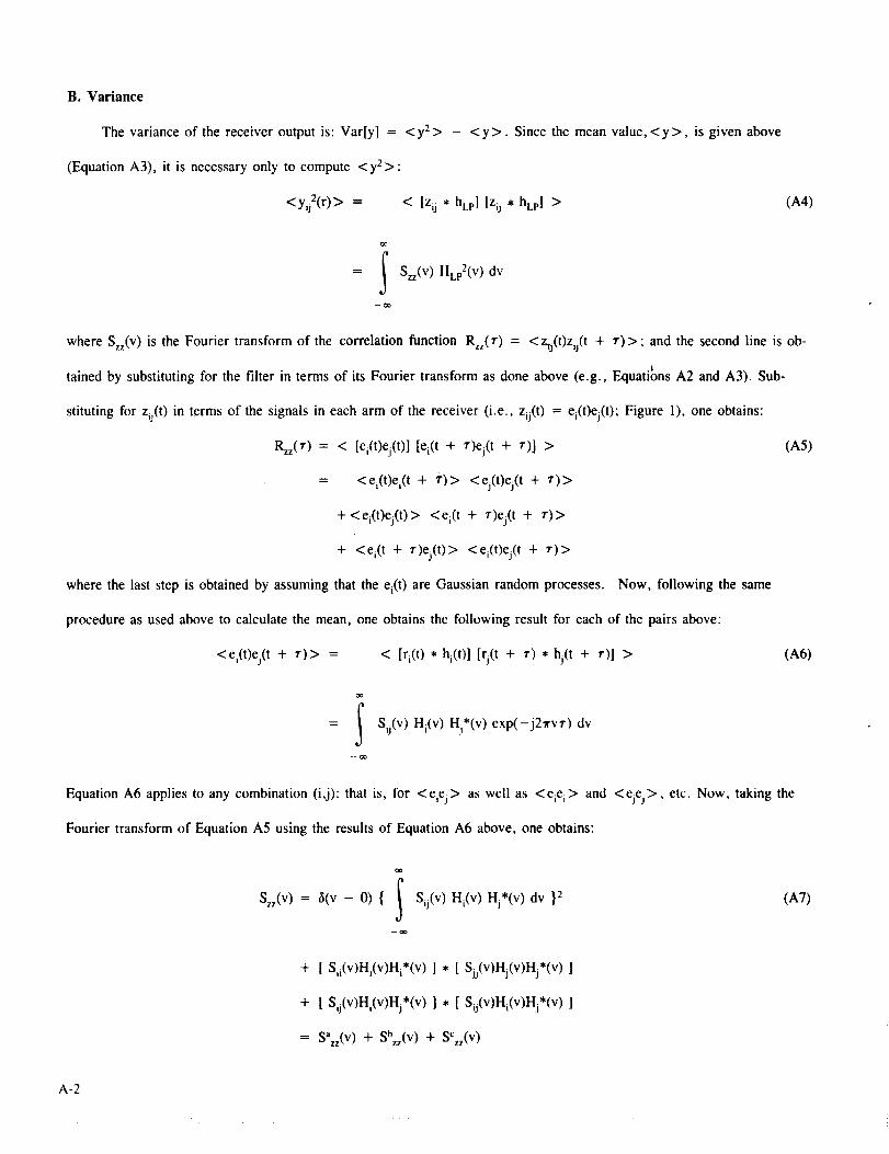
B. Variance

The variance of the receiver output is: Var[y] = <y2> _ <y>. Since the mean value, <y>, is given above

(Equation A3), it is necessary only to compute <y2>:

<yij2(r)> = < [zij * hLp] [zij • hLv] > (A4)

oo

= _I Szz(V) HLp2(V) dv

11

--Oo

where Szz(V)isthe Fouricrtransformof the correlationfunctionRzz(r) = <z_(t)zij(t+ r)>; and thc second lincisob-

.!

tainedby substitutingfor the filterinterms of itsFouriertransformas done above (e.g.,EquatlonsA2 and A3). Sub-

stitutingforzij(t)interms of the signalsineach arm of thc receiver(i.e.,zij(t)= ei(t)cj(t);Figure l),one obtains:

Rzz(r) = < [ei(t)ej(t)] [ei(t + r)ei(t + r)l > (A5)

= <ei(t)ei(t + _')> <ej(t)ej(t + ¢)>

+<ei(t)ej(t)> <ei(t + r)ej(t + r)>

+ <ei(t + r)ej(t)> <ei(t)ej(t + r)>

where the last step is obtained by assuming that the ei(t) are Gaussian random processes. Now, following the same

procedure as used above to calculate the mean, one obtains the following result for each of the pairs above:

<ei(t)ej(t + ¢)> = < [ri(t) * hi(t) l [rj(t + r) * hj(t + r)l > (A6)

ot_

•t Sij(v) Hi(v) Hj*(v)exp(-j2_rvr) dv

oo

Equation A6 applies to any combination (i,j): that is, for <eiej> as well as <eiei> and <ejej>, etc. Now, taking the

Fourier transform of Equation A5 using the results of Equation A6 above, one obtains:

ot_

Szz(v) = _(v - 0) { _t- Sij(V) Hi(v) Hj*(v) dv }2 (A7)

11

--oo

+ [ Sii(v)ai(v)Hi*(v) 1 * [ Sii(v)Hj(v)Hj*(v) 1

+ [ S,j(v)Hi(v)Hj*(v) ! * [ S_j(v)H,(v)Hj*(v) 1

= S_(v) + Sb_(v) + SC_(v)

A-2

Substitutingthisresult(EquationA7) intoEquationA4andcomparingwithEquationA3,oneobtains:

<yij2(r)> = <Yij(r)> 2 +

oo

oo

[Sazz(V) + Sbzz(V)] H2Lp(V)dv

It follows from Equation A8 that:

Var [yij(r)] =

co

[Sbzz(V) + SCzz(V)] H2Lp(v) dv

= [ Sbzz(0) + SCzz(0) ]

oo

I H2Lp(V ) dv

-oo

(A8)

(A9)

The last step in Equation A9 follows because it has been assumed that HLp(v) only passes signals in a narrow band very

close to v = 0. Finally, substituting for the Szz(0) fro.m Equation A7, one obtains:

Var[Yij(r)] = [S2ij(v) + Sii(v)Sjj(v)] H2i(v) H2j(v) dv H2Lp(v) dv (AI0)

The mean and variance of the output of the correlation receiver shown in Figure 1 are given in Equations A3 and

A I0 for a reasonably general set of assumptions. They simplify somewhat in the important, special case when the system

transfer functions Hi(v ) are very narrow compared to the spectra of the input signal, Sij(v), which is the situation encoun-

tered in systems 'designed for microwave remote sensing of the earth from space. In this narrow bandwidth case, the sig-

nal spectra can be factored out of th¢ integrals and one obtains:

oo

/i

< Yij(r) > = Sij(v°) HLp(0) 1 Hi(v) Hj*(v) dv (AI !)

-oo

Var |yij(r)l = [ S2ij(v,,) + Sii(Vo)S.u(vo) ] • J H2i(v ) tt2j(v) dv H2Lp(v) dv (A12)

where % is the center frequency of the filters, Hi(v ). Equations AI ! and A12 are the ones used in the text to compute the

signal-to-noise ratio of the receiver output.

A-3

APPENDIX B

POWER SPECTRUM OF THE ANTENNA OUTPUT VOLTAGES

It is the objective of this appendix to derive an expression for the spectrum of the antenna output voltages (Figure 1)

which are the inputs to the arms of the correlation receiver. In the notation employed in the text this spectrum has been

denoted, < < XiX j > >, where the double brackets < < > > denote a Fourier transform and XiX j is a shorthand notation

for the correlation function<Xi(t)Xi(t + r)>. (In the text, a distinction was made between the response, X °, to a uniform

scene and the response, x i, to fluctuations about this background. In this case one has: X i = X ° + x i. This distinction is

not being made in this appendix and X i is the response of the antenna to an arbitrary scene.) Referring to Figure 1, the Xi,j

are the same as the voltages, Vi,j, at the antenna output terminals; and the discussion in this appendix will be in terms of

the voltages, V(!i,t).

In this appendix, let V(ri t) denote the time-dependent voltage at the output terminal of the antenna at position ri; and

using the same notation as adopted in Appendik "A_,let Sij(v), be the Fourier transform of the correlation function Rij(r) =

< V(ri,(t+ r))V*(rj,t)>. In the special case when the voltages are stationary random processes, one has Sij(v) =

<V(ri,v)V*(rj,v ) > where the V(ri,v) are the Fourier-Stieltjes transforms of the antenna voltages.

In order to obtain expressions for the V(ri,v), imagine two parallel planes, the scene plane which is the source of

the radiation (e.g., the surface of the earth) and a second plane called the image plane at a height H o above the scene

plane. The image plane contains all the interferometer antenna pairs. Let the coordinate origin be in the scene plane and

let r' = + x'_ + y _ + z'_ denote a position in the scene plane (z'=O) and r i = xi_ + Yi_ + zi_ denote the position of

an antenna in the image plane (z i -- Ho). The geometry is illustrated in Figure B1.

It is desired to obtain an expression for the output voltage V(_i,v) from the antenna at _ri in terms of the electric

field, _Es_i',v), on the scene plane. To begin, consider radiation from a small patch Ax' Ay' at r' in the scene plane. The

electric field AE(ri/r',v) radiated from this small patch to the antenna at r i can be obtained from the vector Helmholtz

equation (by assuming that the patch is a small aperture in an otherwise opaque screen on which the tangential compo-

nents of the fields are zero). Following standard procedures (e.g., Tai, 1971), one obtains:

AE(ri/r',v ) = -- { [_ x V X __s(r',v)] *G(_'/_Fi) + [_ x _Es(r',v)]* V x G(_'/ri) } Ax' Ay' (BI)

whcre _ = _ isthe unitvectornormal to the sceneplaneand G(£i/r')isa dyadicGreen's functionsatisfyingthe frec

spacewave equationinthe regionz'> 0. A convenientchoiceforG(f.i/£3is(Tai,1971; Section18):

B-I

_(Li/r')= [T - I/k2VV ][go(_i/_r')- go(Lit_-')] - 2_ go(L/r') (B2)

where T istheunitdyadic,go(L/r_')= exp(jkIr-£' [)/4_rIr-£' I isthe freespace scalarGreen's functionand -_r= £ -

2z_is the "image" of a pointatr behind the sceneplane.The followingpropertiesapply tothisGreen's functionwhen

the sourcepointr' ison the sceneplane:

x _(r'/r)= 0 (B3a)

V' x _'/.r) = _' x 7 go(r '/.r) - _' x _i go([-'/-r) (B3b)

(flx ..E).V'xG_'/r)= 2 (jk - I/R) go([/[')[V R x _ x _) ] (B3c)

Now, noting that [_ x (V x _E) l" _ = -(V x E). [_ x _l and using the preeeeding properties of the dyadic

Green's function, one may write:

AE(Li/r',v ) = 2 (jk - l/R) go(ri/r') [ V R x (_Es x _) l (B4)

The expression in Equation B4. is the signal radiated from the patch on the scene plane to an antenna at ri. The

response of an antenna to radiation from the small patch can be expressed in terms of the voltage transfer function of the

antenna, A(L/r',v), as follows:

AV(r_./_.r',v) = A_E_E(rJr',v) * _A(£/r',v) (B5a)

where the voltage transfer function is a vector quantity to account for the polarization of the antenna (Collin and Zucker,

1969) and can be obtained from the reciprocity theorem for antennas. One can show that A(_/£',v) • A*(r/r',v) =

A_P,(r/L') where A_ is the effective area of the receiving antenna and P,(g./r') is the normalized power pattern of the an-

tenna (Kraus, 1966).

To obtain the response of the antenna to all sources, it is now necessary to sum over all of the scene plane. In the

limit of infinitesimally small patches, the sum approaches an integral and one obtains:

A_.E(ri/r',v ) • A(L.i/r',v ) dr' (ayo)

Eo(r',v),,A(ri/r') [jk - 1/Ri] [zi/R i ]go(Li/_r ') dr' (B5c)

where the radiated electric field in Equation B5c has been expressed in terms of it components, _Eo(r',v) = eh_ + e_',

along horizontally and vertically polarized unit vectors (_, _). These unit vectors are defined locally (i.e. at each point r3

B-2

withrespectto the plane formed by the normal to the surface (_) and the vector, R i = r i - r', from the antenna at r i to

the source point at r'. The unit vectors are:

,,x A

h = (z × V Ri)/sin(Oi) (B6a)

A

v = V R i x (_ × V Ri)/sin(0 i) (B6b)

where sin(0i) = I _ × VRi [ is the angle between the line-of-sight and the z-axis. The projections of the electric field

onto these unit vectors (e h, ev) can be expressed in terms of the field on the surface, Es(L',v), as follows:

A

eh = Es.h cos(0i) (B6c)

e v = [ (Eso_) - (Es.VRi)tan(0i) ] cos(0i) (B6d)

In Equation B4 the factor, cos(0i), appearing above has been factored out and appears explicitly in the form cos(0 i) = zl/R i

where Ri is the magnitude of the vector __Ri and zi = H o (Figure BI). Hence, in Equation B5b one has e h = Es-_ and e_

= _E_._- _,.vK)tan(O,).

Now, using these results and assuming that the distance between the image plane and scene plane is much larger

than the wavelength of any radiation in the passband of interest (i.e., kR i > > 1 for all k of interest) and that the fields

on the surface are (spatially) uncorrelated, one obtains:

S/ , / 2 <A(ri/r, v).I(r' v).A'(r/r v)> exp(jk[R i - Rj]) dr' (B7)Sij(v ) = < V(ri,v)V*_j,v) > = (k o 2x)- (H o RiR j) ....... j_, p

where the dyadic intensity, I(L',v). has been introduced to account for the polarization of the incident radiation. It is

defined as follows:

I(r ',v) = [_Ihh

LI.,

lh_ v

[,,_'

(B8)

where l_b = < e_(r',v) eb*(r',v) >. The brackets < > in the definition tbr lab denote a statistical average over the spa-

tial variable of the random process, and the brackets < >p in Equation B7 indicate an average over polarization states

(Collin and Zucker, 1969).

In the practical cases which are of interest in remote sensing from space, the distance between the scene and image

planes is much larger than the distance between the receiving antennas. In this case one may approximate RiR J in the

B-3

denominatorinEquationB7byRiRj = Ro2, and for the factor R i - Rj appearing in the exponential, one may write

(Appendix C):

R i - Rj = I_ri - r'[ - ]rj - ri[ _ (x i - xj) cos(_x) -+- (Yi - Yj) cos(oty)

where coS(ax,y) are the direction cosines of the vector from the source point at r' in the scene plane to the origin in the

image plane. Using this approximation, one obtains:

(B9)

SS0(v ) = [koHo/2 Ro212 < A(ri/_r',v). ](r',v)-A*(rj/r',v) >p exp[j2r(r/,costx x + r/ycosay)] dr' (BI0)

where

Xi -- Xj

r/x =--v

C

Yi - Yj_r - v (Bll)

c

Ro= I Ho_ - r' l

It is convenient to do the integration in Equation BI0 in terms of the direction cosines cos(Otx,y) rather than in terms

of the coordinates r'. Thus, making the following change of variables:

qx = cos(oq) = x'/Ro(x',y 3

qy = cos(ay) = y'/Ro(x',y')

and using the Jacobian of this transformation dqxdqy = [Ho/Ro2]2dx'dy', one obtains:

(BI2)

+1

SSij(v ) = (1/X 2) < A*I.A*>p exp(j2r__._ dq

-1

A A

where_ = r/_ + r/y_andq = qx x + qyy.

A special case of importance is that in which the antennas are identical and the radiation is unpolarized. Ignoring

the slight difference in location of the antennas (i.e., assuming that A(li/r',v) = A(!j/r',v) ), one obtains:

(B13)

< A.'i-,A*>p = (1/2) A e Pn(q) Ipp(q_) (BI4)

where P,(q...) is the normalized power pattern of the antenna in the direction q (Kraus, 1966), A e is its effective receiving

B-4

area,andIpv(q_)is the spectrum of the electric field on the scene plane with polarization i: Ipp(q) = < [_o_Eo($.,v) ]2 >p.

Hence, in this case:

+1

S_j(v) = (Ae/2k 2) f Pn(q_) Ipp(q_) exp(j2rr/oq) dq (BI5)

-I

In Appendix E it is shown that Ipp(q)/(Zok2) is the brightness in the direction q. Hence,

+I

Sij(v)/Zo = (Ae/2) Pn(q) B(q) exp(j2rr/°q) dq (B16)

-I

where the definition B(q) dq = B(fl) dfl has been made (dl2 = sin(0)d0d_b denotes the "solid angle" in spherical coor-

dinates). It is also shown in Appendix E that B(q_) = B(q) / x/1 - qx2 - qy2. Hence, one may write:

+1

I Pn(q) B(q)Sij(v)/Z o = (A J2) exp(j2rr/oq) dq (B17)_/1 - qx2 - qy2

-I

where B(q_) is now the conventional definition of brightness and Equation B17 is the same as has appeared in the literature

(e.g., Napier et al., 1983). Also, notice that Sij(v)/Z o is the fraction of the power incident on the receiving antenna (per

unit bandwidth) which is available at the antenna output terminals. It is the power which can be delivered to a load

properly matched to the antenna (e.g., Collin and Zucker, 1969).

REFERENCES:

Collin, R.E. and F.J. Zucker (1969), Antenna Theory, Vol. I, Chapter 4, McGraw-Hill Inc.

Kraus, J.D. (1966), Radio Astronomy, Chapter 6, McGraw-Hill Inc.

Tai, C.T. (1971), Dyadic Green's Functions in Electromagnetic Theory, Intext, Pennsylvania.

B-5

\

\ _-t

\\

0"r

x

I.UzILl(0or)

1.1.1

p,,

0

f_

L_

B-6

APPENDIX C

THE SAGITTAL APPROXIMATION

As defined in the previous discussion (Appendix B), r i = x i _ + Yi _ +Ho _ is the position vector of an antenna in

the image plane, r' = x'_ + y _ is the position vector of an arbitrary point on the scene plane, and _R(fi/r _ = r i - r' is

the vector between the point r' on the scene plane and the antenna In this appendix an approxima!e expression for

R(ri/_r ') - R(rj/r ') will be derived where R = I R ] .

Letting _Ro = Ho_-r' and assuming that rti • r_j < R o- where r_i = xi_ + Yi_, one can write:

R(r/.r') - R($j/r') = I ri - r' I - }rj - r'} (Cl)

= I Bo + _r.l - IBo - r,j I (C2)

: _/Ro 2 + rti 2 - 2 Ro.rt i - _/Ro2 + rtj2 _ 2 Ro,rtj (C3)

2 "_ '_

= Ro x/l + (r,_ /Ro-) - 2 _Ro.rJRo'- Ro x/1 + (rcj2/Ro2) - 2 Ro-r_/Ro 2 (C4)

-= (r, 2 - r_j2)/2Ro + Ro.(rt j - rti)/R o (C5)

-= _Ro.(ftj - r,_)/R o (C6)

= (X i -- Xj) COS(Otx) + (Yi -- Yj) COS(Oty) (C7)

where cos(%.y) are the direction cosines of R o (a vector from the source point to the origin in the image plane) with

respect to the coordinate axes in the image plane [cos2(%) + cos2(c_y) + cos2(az) = l ].

In order to use this approximation in the exponential in Equation B7, the error made in replacing Equation C4 by

Equation C6 must be small. Hence, one must have k(ri2 - rj2)/Ro < <ft. As an upper limit on this error one can replace

(ri 2 - rj2) with L 2 where L is the maximum spacing between antennas. Hence, the approximation requires that the size of

the array in the image plane (squared) divided by the minimum distance to the scene plane be much less than a

wavelength. This is a condition easily met in microwave remote sensing of the earth from space (e.g., even in an extreme

case L is not likely to be more than a few 10's of meters, but even in a very low orbit, Ro is on the order of 300 kin or

more).

C-l

APPENDIX D

COORDINATE TRANSFORMATIONS

In this appendix the transformation between the Cartesian coordinates (x', y', z') and the direction cosines (q_ =

cos(Otx); qy = coS(ay); qz = cos(%)) is established. Letting R(x ',y ',z ') = t r'[, one has:

qx =x'/R

qy =y'/R

qz = z'/R

and qx2 + qy2 + qz2 = 1. In the case at hand, z' = Ho is a constant and of interest is the relationship between dx'dy'

and dqxdqy. Using the Jacobian of the transformation to establish the required relationship, one obtains:

dqxdqy =

dqx dqx

dx' dy'

dqy dqy

dx' dy'

dx' dy'

= (H ° / Ro2 )2 dx' dy'

In establishing Equation D3 the following relationships have been used:

dq_/dx = [1 - (x/R)2I/R

dqx/dY = - (xy)/R 3

dqy/dX = -(xy)/R 3

dqy/dy = [1 - (y/R)2]/R

(DI)

(D2)

(D3)

(D4a)

(D4b)

(D4c)

(D4d)

The relationship between the direction cosines (q,,qy) and the spherical coordinates (0,_b) has also been used in the

text. The coordinate transformation is:

q_ = cos(cq) = sin(O) cos(_b)

qy = cos(%) = sin(O) sin(40

(D5)

D-I

PRECEDING PAGE BLANK NOT FILMED

and the Jacobian of the transformation is:

Jacobian =

Thus, one has

dqx

dO

dqy

dO

dq_dqy

dqx

d_

dqy

= sin(O) cos(O) dO d4_

= cos(O) dr/

where df_ = sin(O)dOdO is the differential "solid angle."

The inverse transformation is:

= sin(O) cos(_b)

dfl=dqxdqy

_/1 - q2 _ qy2

(D6)

(D7)

(D8)

D-2

APPENDIX E

RELATIONSHIP BETWEEN BRIGHTNESS AND ELECTRIC FIELD INTENSITY

In the notation commonly used in radio astronomy (e.g., Kraus, 1966), the radiation from a source is defined in

terms of the source "brightness." The brightness is defined to be the power per unit area arriving at the receiver per

steradian from the direction (0,_b) and in a narrow frequency interval, Av. In particular, B(0,4_)sin(0)d0&b = B(fl)df_ is

the power per unit area per unit of bandwidth arriving at the receiver. The radiation received from a thermal source can

be treated as if it were produced by electromagnetic fields on the surface of the source just as radiation from an antenna

can be treated in terms of the equivalent electromagnetic fields on the aperture of the antenna. The objective of this

appendix is to relate B(fl) to these equivalent electromagnetic fields on the surface of the source.

In an electromagnetic system, power is obtained from the Poynting vector, P = E × H. When the observer is very

far from the source, the electromagnetic fields are nearly plane waves and the magnitude of the Poynting vector is ap-

proximately: P = EoE/Z. where Z,, = _ is the characteristic impedance of free space. Assuming that the fields are

ergodic, stationary random processes (in the time coordinate), one obtains:

< P(r,t) > = < E(r,t).E(r,t) > / Z o

oo

= .t P(r,v) dv (El)

--oo

where P(r,v) is the Fourier transform of the autocorrelation function <E_,t)oE(y.,t+r)> evaluated at the position L. It

can also be expressed in terms of the Fourier-Stieltjes transform, E(L,v), in the form: P(r,v) = <_E(r,v)oE*(r.,v)>/Z o. It

follows from Equation E! that the time average power in a frequency band, Av, which is narrow compared to P(.i:,v) is

approximately P(r,v) Av (e.g., Papoulis, 1965).

The spectrum P(£,v) of the radiation at the receiver at r due to a patch of surface at r' can be calculated using the

procedure outlined in Appendix B (letting i = j!. Assuming that the radiation separates in space and time coordinates and

is spatially uncorrelated, one obtains:

P(2,v) dr' _ ' __ = [H,,/R-_/r)I- [I/X2I <_E,(I.',v)'_EI(L',v)/Z,, >p dr' (E2)

E-I

Comparingthisexpressionwiththedefinitionof brightness, one obtains:

B(f_) df_ = P(s.,v) dr' = [l/_k 2] <_.Et(..r',v)o_E,(r',v)>/Z ° _>p [Ho/RZ(_/r')]2 dL' (E3)

Changing from Cartesian to spherical coordinates on the right-hand side in Equation E3, one has [Ho/R2($/r_.')]2dr' =

cos(0) d12. Hence, the relationship between the brightness and the electromagnetic fields on the surface is:

B(fl) = [ i/X 2] [ < E,(12,v)*_E t(12,v) > p/Zo] cos(0) (E4)

The brightness can also be expressed in terms of the direction cosines (q_, %). Defining an alternative brightness, B(q),

and noting thai (Appendix D) dqxd % = (Ho/Ro2) 2 dx'dy', one obtains:

B(q) dq = P_,v) dr' -- [I/'A2][ <Et(q,v)._Et(q,v)>p/Z o ] dq (E5)

Finally, note that

B(q) = B(f_)/cos(0) = B(q)/_/1 - q. 2 _ %. (E6)

REFERENCES:

Kraus, J.D. (1966), Radio Astronomy, McGraw-Hill Inc.

Papoulis, A. (1965), Probability, Random Variables, and Stochastic Processes, Chapter 10, McGraw-Hill, Inc.

E-2

APPENDIX F

THE SYNTHESIZED BEAM

The synthesized beam G(qm .) as defined in the text (Equation 24a) is:

G(q_m,. - q.._)= DFT [ W exp(-j27r_-q._) ] (F1)

where DFT denotes a discrete Fourier transform in two dimensions on the variables (r/x,rly) and w is an arbitrary

"weight" added here to account for biases in the measurements (e.g., differences in the effective time-bandwidth product

or redundancies) or to permit beam shaping to control side lobes. Since the exponential is separable in __, the synthesized

beam G(qm n - q_) also separates and can be factored into the product of two functions: G(qm n - q._) = Gm(qm - qx) o

G,(q, - qy). Each of the Gm,n(qm.n - qx.y) is a one-dimensional, discrete Fourier transform of the exponential

exp(-j2rrr/m,nqx,y). Using the following definition of the discrete Fourier transform

V-_

DFT[ F ] = (l/M) _ F(s) exp(j2r[k/M]s) (F2)

s={M}

each of the one-dimensional transforms can be written as follows:

Gm(qm - qx) = (l/M) Es={M}

W_ exptj27r[(mlM)s - i/_,q_]) (F3a)

G.(q,, - qy) = (I/N) Es={N}

Ys exp(j27r[(n/N)s - _yqyl) (F3b)

Equations F3 can be evaluated explicitly in the important, special case when the measurements are made at (or can be

mapped onto) baselines which are multiples of some minimum spacing d_ and dy in each dimension. The sums in Equa-

F-I

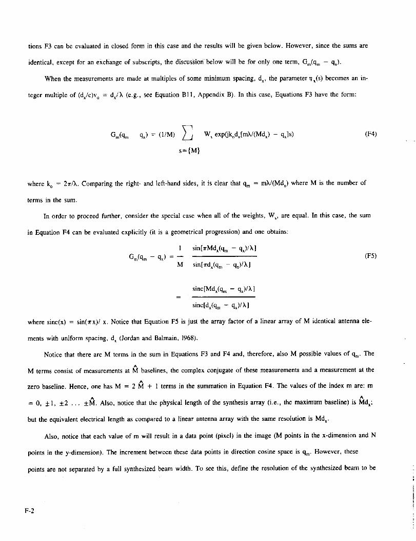
tionsF3canbeevaluatedinclosedformin thiscaseandtheresultswill begivenbelow.However,sincethesumsare

identical,exceptforanexchangeof subscripts,thediscussionbelowwill beforonlyoneterm,Gm(qm- qx)"

When the measurements are made at multiples of some minimum spacing, dx, the parameter r/x(S) becomes an in-

teger multiple of (dx/c)v o = dx/k (e.g., see Equation B11, Appendix B). In this case, Equations F3 have the form:

Gr,(qm - qx) --- (l/M)

s={M}

W s exp(jkodx[mk/(Mdx) - qx]s) (F4)

where ko = 2r/k. Comparing the right- and left-hand sides, it is clear that qm = mX/(Md0 where M is the number of

terms in the sum.

In order to proceed further, consider the special case when all of the weights, W s, are equal. In this case, the sum

in Equation F4 can be evaluated explicitly (it is a geometrical progression) and one obtains:

1 sin[rMdx(qm - qx)/_,]

Gm(qm - qx) = _ (F5)M sin[Trdx(qm - qx)/X]

sinc[Md_(qm - qx)/k]

sinc[dx(qm - qx)/k]

where sinc(x) = sinOrx)/x. Notice that Equation F5 is just the array factor of a linear array of M identical antenna ele-

ments with uniform spacing, d x (Jordan and Balmain, 1968).

Notice that there are M terms in the sum in Equations F3 and F4 and, therefore, also M possible values of qm" The

A

M terms consist of measurements at M baselines, the complex conjugate of these measurements and a measurement at the

A

zero baseline. Hence, one has M = 2 M + 1 terms in the summation in Equation F4. The values of the index m are: m

A A

= 0, + 1, -t-2 ... -t-M. Also, notice that the physical length of the synthesis array (i.e., the maximum baseline) is Mdx;

but the equivalent electrical length as compared to a linear antenna array with the same resolution is Md_.

Also, notice that each value of m will result in a data point (pixel) in the image (M points in the x-dimension and N

points in the y-dimension). The increment between these data points in direction cosine space is qm" However, these

points are not separated by a full synthesized beam width. To see this, define the resolution of the synthesized beam to be

F-2

the distance between the first nulls on each side of the main lobe. Denoting this distance by qo, it is clear from Equation

F5 that:

qo = 2),/Md x =),/D x (F6)

where D x = M dx is the physical length of the array used to synthesize the beam (i.e., the maximum baseline). Since - 1

< qx < + 1 it follows that there are 2/q o = MdxFh = 2Dx/), contiguous resolution cells in the image. On the other hand,

there are a total of M pixels in the reconstructed image in each dimension and each pixel is separated by qm = )'/(Mdx)

(Equation F4). Since qm = 0.o]2 it follows that there are two pixels per resolution cell.

Finally, notice that with uniform weight, grating lobes will appear in the image at integer multiples of ), / d R = qx

(Equation F5). Since - 1 < qx < + 1, one must have ), > dx in order to avoid the presence of grating lobes in the

field of view of the sensor.

REFERENCES:

Jordan, E.C. and K.G. Balmain (1968), Electromagnetic Waves and RadMting Systems, Chapter 12, Prentice-Hall,

Englewood Cliffs, New Jersey.

F-3

Report Documentation PageNat,onal Aeronaulcs andSoace ;_m,n,s1_a_o'_

1. Report No.

NASA TM- i00741

2. Government Accession No.

4. TitleandSubtitle

The Sensitivity of Synthetic Aperture Radiometers for

Remote Sensing Applications From Space

7. Author(s)

D. M. Le Vine

9. Performing OrganizationNameandAddre_

NASA-Goddard Space Flight Center

Greenbelt, Maryland 20771

12. Sponsoring AgencyNameandAddre_

National Aeronautics and Space Administration

Washington, D.C. 20546-0001

3. Recipient's Catalog No.

5. Report Date

December 1989

6. Performing Organization Code

675

8. Performing Organization Report No.

989B00173

10. Work Unit No.

11, Contract or Grant No.

13. Type of Report and Period Covered

Technical Memorandum

14. Sponsoring Agency Code

15. Supplementary Notes

16. Abstract

Aperture synthesis offers a means of realizing the full potential of microwave

remote sensing from space by helPing to overcome the limitations set by antenna

size. The result is a potentially lighter, more adaptable structure for appli-

cations in space. However, because the physical collecting area is reduced, the

signal-to-noise ratio is reduced and may adversely affect the radiometric sensi-

tivity. Sensitivity is an especially critical issue for measurements to be made

from low earth orbit because the motion of the platform (about 7 km/s) limits the

integration time available for forming an image. The purpose of this paper is

to develop expressions for the sensitivity of remote sensing systems which use

aperture synthesis. The objective is to develop basic equations general enough

to be used to obtain the sensitivity of the several variations of aperture syn-

thesis which have been proposed for sensors in space. The conventional microwave

imager (a scanning total power radiometer) is treated as a special case and the

paper concludes with a comparison of three synthetic aperture configurations with

the conventional imager.

17. Key Wo_s(SuggestedbyAuthor(s))Microwave Radiometer

Remote Sensing

Aperture Synthesis

18. DistributionStatement

Unclassified - Unlimited

Subject Category 43

19. SecurityClassif.(ofthisrepo_)

Unclassified

20. SecuriW Classff.(ofthispage)

Unclassified

21. No. of pages

49

22. Price

NASA FORM 1626 OCT 86PRECEDING PAGE BLA_K NOT FILMED