lable at ScienceDirect

Atmospheric Environment 43 (2009) 3596–3604

Contents lists avai

Atmospheric Environment

journal homepage: www.elsevier .com/locate/a tmosenv

The sensitivity of OMI-derived nitrogen dioxide to boundarylayer temperature inversions

Julie Wallace*, Pavlos KanaroglouCentre for Spatial Analysis, School of Geography and Earth Sciences, McMaster University, 1280 Main Street West, Hamilton, Ontario L8S 4L8, Canada

a r t i c l e i n f o

Article history:Received 7 December 2008Received in revised form19 March 2009Accepted 20 March 2009

Keywords:OMINitrogen dioxideTemperature inversions

* Corresponding author. Tel.: þ1 905 525 9140x286E-mail address: wallaju@mcmaster.ca (J. Wallace).

1352-2310/$ – see front matter � 2009 Elsevier Ltd.doi:10.1016/j.atmosenv.2009.03.049

a b s t r a c t

We assess the sensitivity of tropospheric nitrogen dioxide (NO2) derived from the Ozone MonitoringInstrument (OMI), to episodes of temperature inversion in the lower boundary layer. Vertical temper-ature data were obtained from a 91-m meteorological tower located in the study area, which is centeredon the Hamilton Census Metropolitan Area, Ontario, Canada. Hamilton is an industrial city with hightraffic volumes, and is therefore subjected to high levels of pollution. Pollution buildup is amplified byfrequent temperature inversions which are commonly radiative, but are also induced by local physio-graphy, proximity to Lake Ontario, and regional meteorology. The four-year period from January 2005 toDecember 2008 was investigated. Ground-level data for validation were obtained from in situ air qualitymonitors located in the study area. The results indicate that OMI is sensitive to changes in the NO2 levelsduring temperature inversions, and exhibits changes which roughly parallel those of in situ monitors.Overall, an 11% increase in NO2 was identified by OMI on inversion days, compared to a 44% increasemeasured by in situ monitors. The weekend effect was clearly exhibited under both normal and inversionscenarios with OMI. Seasonal and wind direction patterns also correlated fairly well with ground-leveldata. Temperature inversions have resulted in poor air quality episodes which have severely compro-mised the health of susceptible populations, sometime leading to premature death. The rationale for thisstudy is to further assess the usefulness of OMI for population exposure studies in areas with sparseresources for ground-level monitoring.

� 2009 Elsevier Ltd. All rights reserved.

1. Introduction

We investigate the sensitivity of the Ozone Monitoring Instru-ment (OMI) to changes in boundary layer nitrogen dioxide (NO2)during temperature inversion episodes. NO2 is a toxic gas which ispresent in trace amounts in the atmosphere. It exists largely asa secondary pollutant created by oxidation of nitric oxide (NO), a by-product of fuel combustion in transportation and industry. Oxides ofnitrogen, NOx (NO þ NO2) play an integral role in atmosphericchemistry, and reactions are driven by photolysis, concentrations ofother gases, and meteorology (Sillman, 2002; Singh et al., 2007).

Meteorology plays a critical role in dispersion and dilution ofpollution through vertical mixing and horizontal transport. Verticalmixing relies on the upward motion of air. In normal situations, airtemperature decreases with altitude at an average normal lapse rateof about 6.5 �C km�1, creating upward airflow and mixing. If thelapse rate is reversed, a temperature inversion configuration occurs,leading to stable atmospheric conditions with little or no vertical

13.

All rights reserved.

airflow (Oke, 1987). Pollution becomes trapped below the inversioncap, increasing concentrations, sometimes with devastating conse-quences (Holzworth, 1972; Laskin, 2006; Malek et al., 2006).

We investigate the sensitivity of OMI to inversions during2005–2008, based on seasonal, weekday, and various wind direc-tion scenarios. We also test the effect of a negative winter bias inthe OMI data by creating a secondary dataset which excludes thesedata, and comparing with the full dataset. Inversions were identi-fied with vertical temperature data from a 91-m high meteoro-logical tower maintained by the Ontario Ministry of theEnvironment (MOE), in conjunction with Rotek Environmental Inc.,a local environmental company. Ground-level data from in situmonitors were used to validate OMI tropospheric NO2.

2. Study area

The study area spans the region 43.0� N – 43.5� N, 79.5�W – 80.25�

W, and is centered on the Hamilton Census Metropolitan Area (CMA)(Fig. 1). The CMA has a population of 700,000 (Statistics Canada,2008), with the industrial city of Hamilton at its economic core. Thearea is divided physiographically by the Niagara Escarpment,

Fig. 1. Study area indicating 2006 NOx emissions from industry sources, with location of major roads and highways.

J. Wallace, P. Kanaroglou / Atmospheric Environment 43 (2009) 3596–3604 3597

a limestone cuestawhich creates a lower region along the shoreline ofLake Ontario, and an upper plateau. Elevation in the study area rangesfrom 74 m at lake level to 240 m on the plateau.

Temperature inversions occur frequently, and the Escarpmentcontributes to the frequency of advective inversions. Air pollutioncan accumulate to unacceptable levels because of the combinedeffect of emissions from industrial smoke stacks and traffic,impedance of wind flow and pollution dispersion by theEscarpment, and frequent temperature inversions. NOx emissionscontribute to frequent smog alerts in the city, which averaged 30per year between 2002 and 2007 (MOE, 2008). NOx emissionsfrom industry alone exceeded 10,000 tonnes in 2006 (NPRI,2007).

Prevailing winds in the study area are from the SW (50%frequency) with NE and NW winds each occurring with 20%frequency and SE winds with 10% frequency (EC, 2008).

3. Data and methods

3.1. Inversion data

Vertical temperature data were obtained from archived recordsfrom a meteorological tower, Station 29026, located in Hamilton(Fig. 1). Temperatures are measured at heights of 10, 30 and 91 m.Temperature sensors are R. M. Young platinum resistance deviceswith aspirated radiation shields. The instruments are calibratedevery two years as per manufacturer’s specifications. The station ismonitored electronically, and temperatures are recorded eachminute for each 24-h period. Temperature differences between the91 m and 10 m heights were used to determine normal and inversionscenarios. Data for the time period between 13:00 and 14:00 h, forJanuary 2005–December 2008, were selected to coincide with thetime of OMI overpass. A total of 233 daytime inversions and 1211normal scenarios were identified during the study period, thoughthe actual counts used in analyses were constrained by available datafor both OMI and ground monitors. The inversion temperaturegradient between the 10 m and 91 m levels averaged 1.4 �C.

While the inversions identified in this study extend up to 91 m,the caps of the inversions are not known. Inversions may extend

beyond this height or occur in an elevated layer. Well-developedelevated inversions have been identified at altitudes of 1070 m–1980m over the industrial section of Hamilton, by Rouse et al. (1973),using a thermopile transducer mounted on the wing of a Cessna 172aircraft. OMI algorithms determine NO2 in the total troposphericcolumn and do not resolve the effects of inversions based on altitude.However, because tropospheric pollution is driven by anthropogenicemissions in the lowest part of the boundary layer, we anticipate thata buildup of pollution at 0–100 m, could be detected by OMI.

3.2. OMI NO2 tropospheric data

OMI resides on the Aura spacecraft (NASA, 2009) and measuresthe solar radiation backscatter in the range of 270 nm–500 nm,with a spectral resolution of approximately 0.5 nm. The 114�

viewing angle allows daily global coverage with spatial resolutionof 13 � 24 km at nadir. Detailed descriptions of algorithms fortropospheric NO2 retrieval are given in Boersma et al. (2002),Bucsela et al. (2006) and Celarier et al. (2008). Briefly, slant columnsof NO2 are retrieved using differential optical absorption spectro-scopy (DOAS) (Platt, 1994; Eskes and Boersma, 2003) in the 405–465 nm range. This procedure applies a least squares fit ofa modeled spectrum to the natural log of the measured reflectancespectrum. An air mass factor (AMF), defined as the ratio of the slantcolumn density (SCD) to the vertical column density (VCD), isneeded to convert slant to vertical column densities. The StandardProduct (SP) algorithm uses an unpolluted AMF, initially derivedfrom a pre-determined stratospheric NO2 profile. This AMF is usedto generate an initial unpolluted VCD. A GEOS-Chem model ofannual mean tropospheric NO2 (Martin et al., 2003; Bucsela et al.,2006) is used to identify areas within the initial unpolluted fieldthat have pollution levels exceeding 0.5�1015 molec cm�2 (Bucselaet al., 2008). These areas are masked and the remaining data aresmoothed to create a background NO2 field. A positive differencebetween the background field and the initial field indicatestropospheric pollution, which requires an adjustment in the AMF.The polluted AMF is derived from a GEOS-Chem model and is usedto determine the polluted tropospheric VCD.

Fig. 2. Spatial variation of NO2 over the region for 2007, with study area outlined.(Source: GIOVANNI).

J. Wallace, P. Kanaroglou / Atmospheric Environment 43 (2009) 3596–36043598

The use of a mean annual NO2 profile degrades seasonality in theOMI SP data. Lamsal et al. (2008) observed an underestimation ofapproximately 30% in winter NO2 in eastern North America, buta positive bias in rural areas in summer/fall. Irie et al. (2008) alsoobserved a positive bias over the North China Plain in the spring-summer (May–June), and suggest that OMI NO2 could be biased inthe range ofþ20% to�30%. We have also observed a negative winterbias in our data. To assess the effect, given that this bias may coun-teract the positive effect of inversions, a subset of the complete OMIdataset, with winter data excluded, was also analyzed. Results fromthe complete dataset and the winter-excluded dataset are discussed.

OMI Level 2G tropospheric vertical column density NO2 (Version3), for January 2005–December 2008, was acquired using the GES-DISC Interactive Online Visualization ANd aNalysis Infrastructure(GIOVANNI). GIOVANNI was developed by the NASA Goddard EarthSciences (GES) Data and Information Services Center (DISC) andprovides access to OMI SP tropospheric column NO2 data. Thesedata estimate the number of NO2 molecules in an atmosphericcolumn from the Earth’s surface to the top of the troposphere,which is assumed to be at 200 hPa (Celarier et al., 2008, pg 5). TheL2G daily SP is derived from the original Level 2 daily data, andbinned into 0.25� � 0.25� grids. Geometric and geophysical

Table 1Descriptive statistics for NO2 from OMI and CAAQM in situ monitors.

NO2 dataset Number of valid values Minim

a. Full datasetsOMI normal (molec cm�2) 455 1.13EþOMI inversion (molec cm�2) 74 6.48EþCAAQM normal (ppb) 902 2.2CAAQM inversion (ppb) 177 3.2

b. Winter-excluded datasetsOMI normal (molec cm�2) 358 1.13EþOMI inversion (molec cm�2) 62 8.27EþCAAQM normal (ppb) 699 2.17CAAQM inversion (ppb) 115 5.00

parameters for selected data include: viewing angle 0–70�, solarzenith angle 0–88�, and cloud radiance fraction less than 30%. Thedata include only those for which the vcdQualityFlags bit 0 was notset, and thus defined as ‘‘good data’’ values (GIOVANNI, 2009). Timeseries area-averaged NO2 data were acquired to provide daily data,averaged over the study area. Cloud cover is significant in theregion and the OMI data included numerous ‘‘nodata’’ pixels. Forthe 4-year period, valid OMI data were available for 529 days,comprising 455 normal and 74 inversion days. An example of theregional variability of NO2 over the study area and the broaderregion is displayed in Fig. 2.

3.3. Ground-level NO2

Ground-level NO2 data were obtained from three fixed contin-uous ambient air quality monitors (CAAQM) located in the studyarea (Fig. 1). Two monitors are located in close proximity to theindustrial and downtown core of Hamilton, where industry andtraffic are the principal NO2 emitters. The third is located in theTown of Oakville, where traffic is the major source of NO2. Hourlydata for years up to 2007 are currently archived by the MOE (MOE,2008). Daily data for the hour 13:00–14:00 h were selected tocoincide with the time of OMI overpass. At this time of the day, NO2

levels are near the daily minimum in the study area, averagingapproximately 13 ppb, compared to 19 ppb during the morningpeak hour. CAAQM observations provided 1079 valid data dayscomprising 902 normal and 177 inversion values based ontemperature profiles from the meteorological tower.

Surface wind direction and wind speed at 1:00–2:00 pm wereretrieved from Environment Canada archives for the meteorologicalstation located at the Hamilton International Airport (EC, 2008). Adatabase with the integrated daily data for the study period wascreated to include: vertical temperature data, NO2 from both OMI andthe CAAQM, and associated meteorological parameters. The daily datawere tagged with the appropriate month and day of the week.

Statistical analysis using Analysis of Variance (ANOVA) (Turnerand Thayer, 2001), was conducted to test whether the differencesbetween normal and inversion NO2 were statistically significant.The F-statistic, defined as the ratio of the variance between groupsto the variance within group, was used to determine whether themean values are sufficiently different to conclude the unlikelihoodthat they are different by chance. The level of significance wasdetermined at the 5% level of significance.

While data for vertical temperature profiles, meteorology andOMI were available for 2005–2008, the CAAQM data were availableonly for 2005–2007. Because of the limited number of OMI obser-vations, we opted not to restrict the OMI data to 2005–2007 as well.The relatively large number of data values available for the CAAQMmakes it unlikely that this difference in time periods will impactvalidation.

um Maximum Mean Std. Deviation

14 2.33Eþ16 5.10Eþ15 2.86E1514 1.35Eþ16 5.64Eþ15 3.05Eþ15

54.8 11.2 6.140.5 16.1 7.6

14 2.33Eþ16 5.32Eþ15 2.84Eþ1514 1.35Eþ16 6.09Eþ15 2.83Eþ15

39.50 10.53 5.037.33 15.81 7.1

Fig. 3. Frequency of temperature inversions for complete dataset with, a: seasons(JFM: January–March, AMJ: April–June, JAS: July–September, OND: October–November); b: wind direction and wind speed.

J. Wallace, P. Kanaroglou / Atmospheric Environment 43 (2009) 3596–3604 3599

4. Results and discussion

A total of 233 daytime inversions and 1211 normal scenarioswere identified for 2005–2008 (Table 1a). Daytime inversions weremost common in the spring and winter; 36% and 28%, respectively,with 19% and 16% in the summer and fall, respectively (Fig. 3a).Most inversions occurred with the prevailing SW winds (Fig. 3b)

Fig. 4. Regression of OMI versus CAAQM NO2 on normal and inversion days.

and the fewest with SE winds, which also had the lowest windspeeds.

The winter-excluded datasets were reduced by 20% for OMI and25% for the CAAQM (Table 1b). For each set of analyses, we discussfirst the results of the complete dataset, followed by the results ofthe winter-excluded dataset.

Table 1a provides descriptive statistics for NO2 data used in thestudy, for both OMI and CAAQM complete datasets. OMI tropo-spheric column NO2 increased from 5.1Eþ15 to 5.64Eþ15molec cm�2, an increase of 11% on inversion days. CAAQM NO2

averaged 11.2 ppb on normal days and 16.1 ppb on inversion days,a more substantial increase of 44%. ANOVA indicates statisticallysignificant differences in normal and inversion means over the studyperiod for both OMI (p ¼ 0.03) and the CAAQM (p < 0.001).

The large gap between OMI and CAAQM increases is not unex-pected. The CAAQM measures NO2 near the source, and hencerecords higher concentrations. During an inversion episode, theCAAQM is below the inversion cap and measures the full effect ofthe pollution buildup. OMI measures the full tropospheric columnof NO2, over large horizontal extent. Hence, there is more dilutionof surface pollution due to the large volume of air between thesurface and sensor. During inversion episodes, the air above theinversion layer would be less polluted. However, because the totalcolumn is measured and tropospheric pollution is driven byemissions at or near the surface, NO2 beneath the inversion capwould also be detected by OMI, but at lower concentrations.

Regression coefficients for plots of OMI NO2 versus CAAQM NO2,(Fig. 4) produce a better fit on inversion days (R2 ¼ 0.35), comparedto normal days (R2 ¼ 0.20). This may be indicative of a moreaccurate measure of NO2 by OMI when stable atmospheric condi-tions prevail. Under stable conditions, dispersion and verticalmixing are reduced, so that the pollution recorded by the large OMIfield of view is more consistent with that measured on the ground.

The winter-excluded dataset resulted in a further 3% increase inOMI NO2 (from 11 to 14%), and 6% increase in CAAQM NO2 (from 44

Fig. 5. Seasonal comparison of NO2 from a: OMI and b: CAAQM during inversion andnormal scenarios.

Table 2Seasonal means of NO2 from OMI and CAAQM in situ monitors, for inversion and normal scenarios, with ANOVA statistics for normal and inversion means (JFM-winter,AMJ-spring, JAS-summer, OND-fall).

Month NO2 Number of days ANOVA Statistics, (5% level)

Inversion Normal % Increase Inversion days Normal days F p

OMI NO2 (�1015 molec cm�2)JFM 4.61 4.19 10 20 92 4.5 0.55AMJ 5.92 5.65 5 31 125 0.3 0.61JAS 5.17 4.66 11 10 145 2.4 0.09OND 8.15 5.91 38 13 93 0.4 0.04

CAAQM NO2 (ppb)JFM 16.7 13.5 24 62 203 6.9 <0.001AMJ 15.8 10.6 50 65 208 43.8 <0.001JAS 12.4 8.5 46 27 246 30.4 <0.001OND 19.7 12.5 57 23 245 6.9 <0.001

J. Wallace, P. Kanaroglou / Atmospheric Environment 43 (2009) 3596–36043600

to 50%) on inversion days (Table 1b). ANOVA indicates statisticallysignificant differences for both OMI (p ¼ 0.02) and the CAAQM(p < 0.001). Mean OMI NO2 increased for both normal and inver-sion scenarios, while both CAAQM means decreased, whencompared to the full dataset.

4.1. NO2 and seasons

Seasons were defined as: winter – January to March, spring – Aprilto June, summer – July to September, and fall – October to December.OMI displayed consistently higher NO2 levels during inversionscenarios (Fig. 5), with modest increases of 5–11% in the winter,spring and summer and a considerably higher increase of 38% in thefall (Table 2). Lowest NO2 levels for both normal and inversion dayswere observed in the winter and summer. The CAAQM also identifiedseasonal increases during inversions, ranging from 24% in the winterto 57% in the fall. ANOVA indicate statistically significant differencesbetween OMI NO2 during normal and inversion scenarios for the fallonly, while the differences were significant for all seasons for theCAAQM (Table 2).

While there are similarities in the summer and fall patterns ofthe CAAQM and OMI data, a general conclusion cannot be drawn onthe sensitivity of OMI with regards to the seasons. The OMI winterand spring variations deviate significantly from observed grounddata. Typically, eastern North America experiences highest NO2

levels in winter because of the longer lifetime and the lower mixing

Fig. 6. Monthly concentrations of NO2 from a: OMI (2005–2008) and b: CAAQM(2005–2007), showing different patterns of seasonal variations in the datasets.

height (Lamsal et al., 2008). NO2 minima are experienced in thesummer. Obvious differences in the OMI and CAAQM seasonal data(Fig. 5) are the OMI winter minimum and spring peak, compared tothe CAAQM winter maximum and lower spring values. Theseseasonal variations are more clearly illustrated in the integratedNO2 datasets (no separation of normal and inversion days) for OMIand the CAAQM (Fig. 6). The CAAQM reflect the more accurateseasonal variation, with a winter maximum and summerminimum. The differences can be explained, in part, by the algo-rithms used to retrieve the OMI SP tropospheric VCD, as previouslyexplained.

Re-analysis of the seasonal data with the winter-excludeddataset was not necessary, as the results remain as seen in Table 2,ignoring the winter results.

4.2. NO2 and weekdays

The ‘‘weekend effect’’ is evident in both OMI and CAAQMcomplete datasets (Fig. 7). This effect, which describes a reductionin pollution levels on weekends in response to decreased trafficvolumes, has previously been observed with ground data (e.g. Elkusand Wilson, 1977; Murphy et al., 2007) and satellite data (Beirle

Fig. 7. Comparison of NO2 from complete dataset; a: OMI and b: CAAQM on inversionand normal weekdays, with standard error bars.

Table 3Weekday mean NO2 from OMI and CAAQM in situ monitors, for inversion and normal scenarios, with ANOVA statistics for normal and inversion means.

Weekday NO2 Number of days ANOVA (5% level) ANOVA (5% level)

Inversion Normal % increase Inversion Normal F p Fa Pa

OMI NO2 (�1015 molec cm�2)2005–2008 5.64 5.10 11 74 455 4.3 0.03 5.9 0.02Sunday 4.15 3.44 21 8 70 1.9 0.15 0.9 0.35Monday 5.68 4.91 16 12 60 1.9 0.16 1.9 0.18Tuesday 6.93 6.01 15 11 61 0.7 0.50 3.5 0.07Wednesday 6.99 5.61 25 14 66 3.1 0.08 0.8 0.37Thursday 7.04 5.89 20 11 56 1.1 0.29 0.6 0.46Friday 6.61 5.65 17 9 68 0.8 0.36 0.3 0.60Saturday 2.36 4.48 �47 9 74 4.5 0.01 1.4 0.23

CAAQM NO2 (ppb)2005–2007 16.1 11.19 44 177 901 88.8 <0.001 94.8 <0.001Sunday 11.8 8.0 47 30 123 15.0 <0.001 8.3 <0.001Monday 18.3 11.9 54 31 124 21.5 <0.001 22.7 <0.001Tuesday 17.5 12.8 37 23 132 9.4 <0.001 13.8 <0.001Wednesday 17.6 12.2 44 29 124 21.6 <0.001 25.6 <0.001Thursday 19.4 12 62 24 131 37.2 <0.001 27.3 <0.001Friday 18.7 12.0 55 18 137 17.9 <0.001 25.3 <0.001Saturday 9.8 9.3 5 22 131 0.01 0.72 0.4 0.55

a Winter-excluded dataset.

J. Wallace, P. Kanaroglou / Atmospheric Environment 43 (2009) 3596–3604 3601

et al., 2003; Bucsela et al., 2007; Wallace and Kanaroglou, 2008).We observed that OMI is also sensitive to the changes in NO2 oninversion days, and displays increased inversion day levels whilemaintaining the weekend effect (Fig. 7a). This response is validatedby the CAAQM data which display a very similar pattern (Fig. 7b),with an increase in inversion day NO2 for each day of the week.Both datasets display a sharp decline in the inversion NO2 onSaturdays. The decreased weekend traffic activity appears to lowerinversion buildup considerably. OMI inversion day increases rangedfrom 15 to 25%, with the exception of a 47% decrease on Saturdays(Table 3). The CAAQM increases were higher, ranging from 37% to62% with a low of 5% on Saturdays. The stronger effect in theCAAQM stems from their closer proximity to NO2 traffic andindustry sources. Standard error bars indicate relatively low stan-dard errors in the data (Fig. 7).

ANOVA indicates that weekday differences were not statisticallysignificant for OMI, with the exception of Saturday, which exhibitedvery low inversion day NO2 (Table 3). CAAQM data producedsignificant differences for all days except Saturday.

Fig. 8. Up-down bars showing normal and inversion NO2 for weekdays; a: OMI complete daLight grey bars indicate an increase on inversion days and dark grey bars indicate a decrea

Re-analysis of weekday data with the winter-excluded datasetdemonstrates that the weekend effect remained clearly defined ininversion and normal scenarios, for both reduced datasets.OMI NO2 (Fig. 8a, b) was higher for the winter-excluded datasetwhen compared to the complete dataset, for both inversion andnormal scenarios, for all days. CAAQM NO2 however, was lower forall normal days, since the excluded winter values were high (Fig. 8c,d), and displayed a mix of higher and lower values on inversiondays. ANOVA results for OMI NO2 were consistent with those of thefull dataset with one exception on Saturdays (Table 3), whichbecomes non-significant because of the less decreased inversionvalues (Fig. 8a, b). ANOVA results for the reduced CAAQM data wereconsistent with that of the complete dataset (Table 3).

4.3. NO2 and wind direction

Both OMI and the CAAQM identify the lowest NO2 levels withNW winds for both normal and inversion scenarios, and bothassociate highest NO2 levels with SE winds (Table 4, Fig. 9a, c). OMI,

taset, b: OMI winter removed, c: CAAQM complete dataset, d: CAAQM winter removed.se.

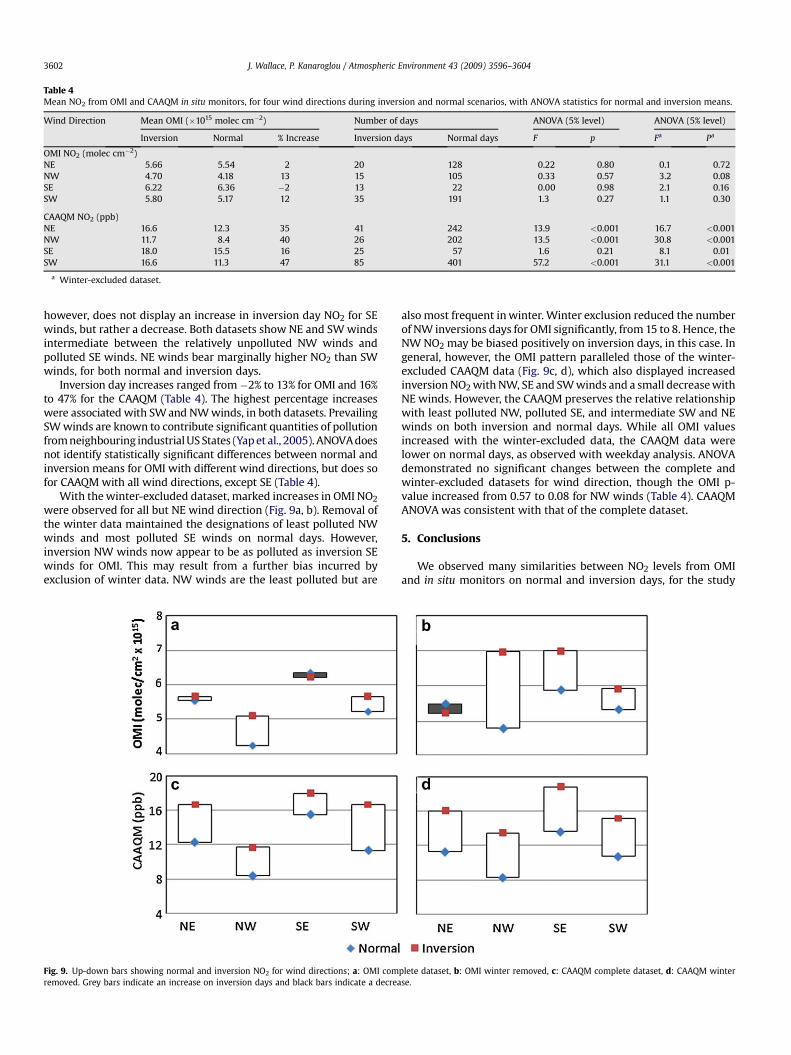
Table 4Mean NO2 from OMI and CAAQM in situ monitors, for four wind directions during inversion and normal scenarios, with ANOVA statistics for normal and inversion means.

Wind Direction Mean OMI (�1015 molec cm�2) Number of days ANOVA (5% level) ANOVA (5% level)

Inversion Normal % Increase Inversion days Normal days F p Fa Pa

OMI NO2 (molec cm�2)NE 5.66 5.54 2 20 128 0.22 0.80 0.1 0.72NW 4.70 4.18 13 15 105 0.33 0.57 3.2 0.08SE 6.22 6.36 �2 13 22 0.00 0.98 2.1 0.16SW 5.80 5.17 12 35 191 1.3 0.27 1.1 0.30

CAAQM NO2 (ppb)NE 16.6 12.3 35 41 242 13.9 <0.001 16.7 <0.001NW 11.7 8.4 40 26 202 13.5 <0.001 30.8 <0.001SE 18.0 15.5 16 25 57 1.6 0.21 8.1 0.01SW 16.6 11.3 47 85 401 57.2 <0.001 31.1 <0.001

a Winter-excluded dataset.

J. Wallace, P. Kanaroglou / Atmospheric Environment 43 (2009) 3596–36043602

however, does not display an increase in inversion day NO2 for SEwinds, but rather a decrease. Both datasets show NE and SW windsintermediate between the relatively unpolluted NW winds andpolluted SE winds. NE winds bear marginally higher NO2 than SWwinds, for both normal and inversion days.

Inversion day increases ranged from �2% to 13% for OMI and 16%to 47% for the CAAQM (Table 4). The highest percentage increaseswere associated with SW and NW winds, in both datasets. PrevailingSW winds are known to contribute significant quantities of pollutionfrom neighbouring industrial US States (Yap et al., 2005). ANOVA doesnot identify statistically significant differences between normal andinversion means for OMI with different wind directions, but does sofor CAAQM with all wind directions, except SE (Table 4).

With the winter-excluded dataset, marked increases in OMI NO2

were observed for all but NE wind direction (Fig. 9a, b). Removal ofthe winter data maintained the designations of least polluted NWwinds and most polluted SE winds on normal days. However,inversion NW winds now appear to be as polluted as inversion SEwinds for OMI. This may result from a further bias incurred byexclusion of winter data. NW winds are the least polluted but are

Fig. 9. Up-down bars showing normal and inversion NO2 for wind directions; a: OMI comremoved. Grey bars indicate an increase on inversion days and black bars indicate a decrea

also most frequent in winter. Winter exclusion reduced the numberof NW inversions days for OMI significantly, from 15 to 8. Hence, theNW NO2 may be biased positively on inversion days, in this case. Ingeneral, however, the OMI pattern paralleled those of the winter-excluded CAAQM data (Fig. 9c, d), which also displayed increasedinversion NO2 with NW, SE and SW winds and a small decrease withNE winds. However, the CAAQM preserves the relative relationshipwith least polluted NW, polluted SE, and intermediate SW and NEwinds on both inversion and normal days. While all OMI valuesincreased with the winter-excluded data, the CAAQM data werelower on normal days, as observed with weekday analysis. ANOVAdemonstrated no significant changes between the complete andwinter-excluded datasets for wind direction, though the OMI p-value increased from 0.57 to 0.08 for NW winds (Table 4). CAAQMANOVA was consistent with that of the complete dataset.

5. Conclusions

We observed many similarities between NO2 levels from OMIand in situ monitors on normal and inversion days, for the study

plete dataset, b: OMI winter removed, c: CAAQM complete dataset, d: CAAQM winterse.

J. Wallace, P. Kanaroglou / Atmospheric Environment 43 (2009) 3596–3604 3603

period. Tropospheric column NO2 measured by OMI appears to besensitive to the changes in NO2 concentrations at ground levelwhen an inversion occurs in the lowest 100 m of the boundarylayer. OMI NO2 increases on inversion days are less than observed inCAAQM data, as expected, since OMI measures more diluteconcentrations over larger vertical and horizontal extent.

OMI discriminated the ‘‘weekend effect’’ on normal and inversiondays, with temporal patterns that parallel those observed with theCAAQM. OMI observations with wind direction were largely consis-tent with those of the CAAQM, with highest NO2 associated with SEwinds, and least with NW winds. Seasonal increases were apparentbut less conclusive because of the negative bias in winter data.

Removal of the winter data from both datasets enhanced theoverall inversion day increases by 3% for OMI and 6% for theCAAQM. The weekend effect was preserved with the winter-excluded datasets and OMI results for wind direction roughlyparalleled those of the CAAQM. However, the winter exclusionbiased wind direction data, since the least polluted NW winds aremost frequent in winter. Overall, OMI NO2 increased with thewinter-excluded dataset for both normal and inversion scenariossince the negatively biased data were removed. CAAQM decreasedfor normal days because the winter highs were removed, andexperienced a mix of higher and lower values on inversion days.

Differences in OMI and CAAQM data may be attributed to manyfactors. OMI measures the tropospheric column with pixel resolu-tion ranging from13 � 24 km at nadir to 26 � 128 km at the outerswath angle, compared to the point concentrations measured bythe CAAQM at ground level. OMI measurements represent largespatial extent and include areas of high and low anthropogenicpollution. The study area includes polluted urban environments,rural areas and a portion of Lake Ontario, the latter two being lesspolluted areas. Shipping traffic associated with the local steelindustry contributes to NO2 over Lake Ontario, as do industrieslocated near the shoreline. While the magnitude of this contribu-tion is not known, it will be lower than that of the heavily traffickedareas, adding to the spatial heterogeneity. Another factor is thatwind directions used in these analyses are measured at one locationat surface, and do not account for conditions elsewhere or in thetropospheric column.

Retrieval of VCD from the measured radiance is complex anderrors in geophysical and geometric parameters, such as cloudcover and surface albedo, a priori NO2 profiles, and variability in thevertical distribution of NO2, add to the error budget (Boersma et al.,2004; Celarier et al., 2008).The use of an annual mean profile todetermine OMI VCD diminishes seasonality in the OMI SP data.Errors are also higher in polluted environments (Boersma et al.,2002). Spatial and temporal heterogeneity in the NO2 field, asobserved by Brinksma et al. (2008) add to the uncertainties.

Recent studies suggest that interference errors associated withNO2 measurements from commercial chemiluminescenceanalyzers, such as those used by the MOE, could account for up to22% of recorded NO2 in polluted environments (Dunlea et al., 2007;Lamsal et al., 2008). This overestimation further degrades therelationship between OMI and ground data.

Despite the fact that OMI data are confounded by many factors,it is encouraging that the general patterns of change discriminatedduring temperature inversions are very similar to those observed inthe CAAQM data. OMI appears to be sensitive, not only to thetemporal distribution of NO2 but also to the subtle changes causedby temperature inversions, even when accounting for a negativewinter bias in the OMI data. The results complement other studieswhich conclude that OMI can be used to estimate ground-level NO2

(Lamsal et al., 2008; Martin, 2008) and support the feasibility ofusing OMI for regional pollution studies, particularly whereground-level monitors are not available.

Acknowledgements

The authors would like to thank the Ontario Ministry of theEnvironment and Rotek Environmental Inc. for access to themeteorological tower data. We also thank two anonymousreviewers for helpful comments on the manuscript.

References

Beirle, S., Platt, U., Wenig, M., Wagner, T., 2003. Weekly cycle of NO2 by GOMEmeasurements: a signature of anthropogenic sources. Atmospheric Chemistryand Physics 3, 2225–2232.

Boersma, K.F., Bucsela, E.J., Brinksma, E.J., Gleason, J.F., 2002. NO2. In: Chance, K.(Ed.), OMI Algorithm Theoretical Basis Document, OMI Trace Gas Algorithms.ATB OMI-04, Version 2.0, vol. 4. NASA Distributed Active Archive Centers,Greenbelt, MD, pp. 13–36.

Boersma, K.F., Eskes, H.J., Brinksma, E.J., 2004. Error analysis for troposheric NO2retrieval from space. Journal of Geophysical Research 109, D04311, doi:10.1029/2003JD003962.

Brinksma, E.J., et al., 2008. The 2005 and 2006 DANDELIONS NO2 and aerosolintercomparison campaigns. Journal of Geophysical Research 113, D16S46,doi:10:1029/2007JD008808.

Bucsela, E.J., Celarier, E.A., Wenig, M.O., Gleason, J.F., Veefkind, J.P., Boersma, K.F.,Brinksma, E.J., 2006. Algorithm for NO2 vertical column retrieval from theOzone Monitoring Instrument. IEEE Transactions Geoscience and RemoteSensing 44, 1245–1258, doi:10.1109/TGRS.2005.863715.

Bucsela, E.J., Wenig, M.O., Celarier, E.A., Gleason, J.F., 2007. The ‘‘WeekendEffect’’ in Tropospheric NO2 Seen from the Ozone Monitoring Instrument.Abstracts, American Geophysical Union Fall Meeting, San Francisco,December 2007.

Bucsela, E.J., Perring, A.E., Cohen, R.C., Boersma, K.F., Celarier, E.A., Gleason, J.F.,Wenig, M.O., Bertram, T.H., Wooldridge, P.J., Dirksen, R., Veefkind, J.P., 2008.Comparison of tropospheric NO2 from in situ aircraft measurements with near-real-time and standard product data from OMI. Journal of Geophysical Research113, D16S31, doi:10.1029/2007JD008838.

Celarier, E.A., Brinksma, E.J., Gleason, J.F., Veefkind, J.P., Cede, A., Herman, J.R.,Ionov, D., Goutail, F., Pommereau, J.P., Lambert, J.C., van Roozendael, M.,Pinardi, G., Wittrock, F., Schonhardt, A., Richter, A., Ibrahim, O.W., Wagner, T.,Bojkov, B., Mount, G., Spinei, E., Chen, C.M., Pongetti, T.J., Sander, S.P.,Bucsela, E.J., Wenig, M.O., Swart, D.P.J., Volten, H., Kroon, M., Levelt, P.F., 2008.Validation of Ozone Monitoring Instrument nitrogen dioxide columns. Journalof Geophysical Research 113, D15S15, doi:10.1029/2007JD008908.

Dunlea, E.J., Herndon, S.C., Nelson, D.D., Volkamer, R.M., San Martini, F.,Sheehy, P.M., Zahniser, M.S., Shorter, J.H., Wormhoudt, J.C., Lamb, B.K.,Allwine, E.J., Gaffne, J.S., Marley, N.A., Grutter, M., Marquez, C., Blanco, S.,Cardenas, B., Retama, A., Ramos Villegas, C.R., Kolb, C.E., Molina, L.T.,Molina, M.J., 2007. Evaluation of nitrogen dioxide chemiluminescence monitorsin a polluted urban environment. Atmospheric Chemistry and Physics 7,2691–2704.

Environment Canada, 2008. National Climate Data and Information Archive. Envi-ronment Canada. Online. http://climate.weatheroffice.ec.gc.ca/ (accessedAugust, 2008).

Elkus, B., Wilson, K.R., 1977. Photochemical air pollution: weekend-weekdaydifferences. Atmospheric Environment 11, 509–515.

Eskes, H.J., Boersma, K.F., 2003. Averaging kernels for DOAS total-column satelliteretrievals. Atmospheric Chemistry and Physics 3, 1285–1291.

GIOVANNI, 2009. Giovanni 3 Online Users Manual. Online. http://disc.sci.gsfc.nasa.gov/giovanni/ (accessed January 2009).

Holzworth, G.L., 1972. Vertical temperature structure during the thanksgivingweek air pollution episode in New York City. Monthly Weather Review 100,445–450.

Irie, H., Kanaya, Y., Akimoto, H., Tanimoto, H., Wang, Z., Gleason, J.F., Bucsela, E.J.,2008. Validation of OMI tropospheric NO2 column data using MAX-DOASmeasurements deep inside the North China Plain in June 2006: Mount TaiExperiment 2006. Atmospheric Chemistry and Physics 8, 6577–6586.

Lamsal, L.N., Martin, R.V., van Donkelaar, A., Steinbacher, M., Celarier, E.A.,Bucsela, E., Dunlea, E.J., Pinto, J.P., 2008. Ground-level nitrogen dioxideconcentrations inferred from the satellite-borne Ozone Monitoring Instrument.Journal of Geophysical Research 113, D16308, doi:10.1029/2007JD009235.

Laskin, D., 2006. The Great London smog. Weatherwise 59, 42–45.MOE, 2008. Air quality Ontario. Online. http://www.airqualityontario.com

(accessed November 2008).Malek, E., Davis, T., Martin, R.S., Silva, P.J., 2006. Meteorological and environmental

aspects of one of the worst national air pollution episodes (January, 2004) inLogan, Cache Valley, Utah, USA. Atmospheric Research 79, 108–122.

Martin, R.V., 2008. Satellite remote sensing of surface air quality. AtmosphericEnvironment 42, 7823–7843.

Martin, R.V., Jacob, D.J., Yantosca, R.M., Chin, M., Ginoux, P., 2003. Global andregional decreases in tropospheric oxidants from photochemical effects ofaerosols. Journal of Geophysical Research 108 (D3), 4097, doi:10.1029/2002JD002622.

J. Wallace, P. Kanaroglou / Atmospheric Environment 43 (2009) 3596–36043604

Murphy, J.G., Day, D.A., Cleary, P.A., Wooldridge, P.J., Millet, D.B., Goldstein, A.H.,Cohen, R.C., 2007. The weekend effect within and downwind of Sacramento:Part 1. Observations of ozone, nitrogen oxides, and VOC reactivity. AtmosphericChemistry and Physics 7, 5327–5339.

NASA, 2009. The National Aeronautics and Space Administration Aura Mission. Online.http://www.nasa.gov/mission_pages/aura/spacecraft/omi.html (accessed July 2008).

NPRI, 2007. The National Pollution Release Inventory. Environment Canada. Online.http://www.ec.gc.ca/pdb/npri/ (accessed August 2008).

Oke, T.R., 1987. Boundary Layer Climates, second ed. Routledge.Platt, U., 1994. Differential Optical Absorption Spectroscopy (DOAS). In: Sigrist, M.

(Ed.), Air Monitoring by Spectroscopic Techniques. John Wiley, Hoboken, NewJersey, pp. 27–84.

Rouse, W.R., Noad, D., McCutcheon, J., 1973. Radiation, temperature and atmo-spheric emissivities at a polluted urban atmosphere in Hamilton, Ontario.Journal of Applied Meteorology 12, 798–807.

Sillman, S., 2002. The relation between Ozone, NOx and hydrocarbons in urban andpolluted rural environments. In: Brimblecombe (Ed.), Air Pollution Science for the21st Century, Developments in Environmental Science Series 1. Elsevier, Oxford.

Singh, H.B., Salas, L., Herlth, D., Kolyer, R., Czech, E., Avery, M., Crawford, J.H.,Pierce, R.B., Sachse, G.W., Blake, D.R., Cohen, R.C., Bertram, T.H., Perring, A.,Wooldridge, P.J., Dibb, J., Huey, G., Hudman, R.C., Turquety, S., Emmons, L.K.,Flocke, F., Tang, Y., Carmichael, G.R., Horowitz, L.W., 2007. Reactive nitrogendistribution and partitioning in the North American troposphere and lower-most stratosphere. Journal of Geophysical Research 112, D12S04, doi:10.1029/2006JD007664.

Statistics Canada, 2008. Census of Canada. Online. http://www12.statcan.ca/english/census/index.cfm (accessed July 2008).

Turner, J.R., Thayer, J., 2001. Introduction to Analysis of Variance. Sage Publications,Thousand Oaks, CA.

Wallace, K., Kanaroglou, P., 2008. Weekday and seasonal variations in NO2 isSouthern Ontario, Canada, using data from the ozone monitoring instrument(OMI). In: IEEE Proceedings of the International Symposium on Geoscience andremote sensing July 6–11, 2008, Boston.

Yap, D., Reid, N., De Brou, G., Bloxam, R., 2005. Transboundary Air Pollution inOntario. Ontario Ministry of the Environment Report. PIBS, Toronto, Ontario.p. 5158e.